Does the marine biosphere mix the ocean?

Does the marine biosphere mix the ocean

by W K Dewar12 R J Bingham3 R L Iverson1 D P Nowacek1L C St Laurent1 and P H Wiebe4

ABSTRACTOcean mixing is thought to control the climatically important oceanic overturning circulation

Here we argue the marine biosphere by a mechanism like the bioturbation occurring in marinesediments mixes the oceans as effectively as the winds and tides This statement is derivedultimately from an estimated 627 TeraWatts of chemical power provided to the marine environmentin net primary production Various approaches argue something like 1 (63 TeraWatts) of thispower is invested in aphotic ocean mechanical energy a rate comparable to wind and tidal inputs

1 Introduction

The deep waters of the world ocean are stratified and in an insightful paper Munk andWunsch (1998 MW98 hereafter) revisited the question of how this stratification ismaintained Ultimately the discussion in MW98 turned to turbulent mechanical energy andthe power sources driving that turbulence The inputs to this energy of physical origin haveby now been rather thoroughly examined we here take a different approach and suggestthat a source of biologicalchemical origin ie the marine biosphere is plausibly ofcomparable importance to the turbulent mechanical energy budget

a Background

A well-known feature of the ocean circulation is its meridional overturning cell (MOChereafter see Fig 1) which is in turn intimately connected with the deep stratificationThere are two thoughts about how the MOC is maintained One view originally advancedby Toggweiler and Samuels (1998) and Webb and Suginohara (2001) focuses on thesurface effects of the wind in the Southern Ocean The other view discussed in MW98 andmore recently in Wunsch and Ferrari (2004) emphasizes the importance of turbulentmixing in which heat mixed downward warms mid-latitude abyssal waters and drives anupwelling that balances high latitude deep water formation While both processes areprobably in operation which one is dominant is not yet clear

1 Department of Oceanography Florida State University Tallahassee Florida 32306 USA2 Corresponding author email dewaroceanfsuedu3 Proudman Oceanographic Laboratory 6 Brownlow Street Liverpool L35DA United Kingdom4 Biology Department Woods Hole Oceanographic Institution Woods Hole Massachusetts 02543 USA

Journal of Marine Research 64 541ndash561 2006

541

The mixing scenario in MW98 framing the discussion here most likely determines thedeeper stratification and thus a component of the MOC This has climatic implicationsthrough climate-MOC connections and in part motivates the present work Crudelyspeaking climate is a by-product of a global transport of excess heat from the equator tothe poles While their ratio is debated the atmosphere and ocean are comparablecontributors to this transport (Trenberth and Caron (2001) argue that the atmosphere is theprimary contributor and the ocean secondary) and in the ocean the MOC is important forheat flux MOC variability then potentially connects to climate variability possiblyimprinting time scales from years to millennia on the system and synchronizing pastglaciations (Broecker and Denton 1989)

It is also clear that ocean diapycnal mixing in its vertical transport of buoyancy mustconsume energy MW98 estimate the mixing power requirement at about 2 Terawatts(1 TW 1012 W) Although this number is likely uncertain to a factor of two St Laurentand Simmons (2006) use an independent technique and find a comparable if modestlyhigher bulk dissipation (24 TW) To obtain the total energy flux through the systemthese numbers must be augmented by an additional 20 (reflecting an assumed mixingefficiency of 02) to account for the increase in potential energy associated with themixing yielding a total power requirement of 29 TW Again this number contains largeerror bars MOC dependence on mixing differs importantly from classical scaling whenenergetics constraints are considered (Huang 1998)

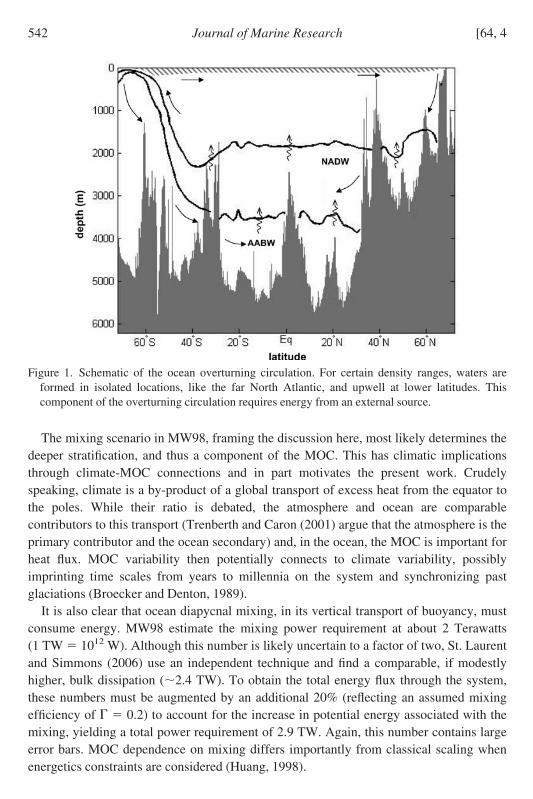
Figure 1 Schematic of the ocean overturning circulation For certain density ranges waters areformed in isolated locations like the far North Atlantic and upwell at lower latitudes Thiscomponent of the overturning circulation requires energy from an external source

542 [64 4Journal of Marine Research

A central issue in the study of mixing then has become the identification of the energysources providing the needed power Indeed this is part of the broader open question ofthe ocean energy budget the clarification of which is of obvious scientific value Heatingand cooling have traditionally been thought to provide the sources of energy for the MOCbut theory suggests otherwise (Sandstrom 1916 Paparella and Young 2002) MW98instead argue winds and tides provide about 1 TW each to mixing resulting in a total powerthat is a substantial fraction and perhaps all of the energy apparently needed to mix thedeep ocean With one possible exception other physical sources like geothermal heatingappear to be weak (Huang 1999 Wunsch and Ferrari 2004) The exception is themesoscale whose energy is ultimately provided by the large-scale winds Wunsch (1998)estimates energy moves through the mesoscale at a rate of about 1 TW How this energygets out of the mesoscale is however unclear and it is unknown if this is a significantcontributor to the turbulent ocean mechanical energy budget

Although sources yielding net power close to the apparent requirement have beenidentified there are several reasons to believe the budget is not yet balanced For exampleit is not clear if all the energy lost to the ocean from the winds and tides is spent on mixingBaroclinic tides are generated with vertical scales of kilometers whereas dissipation in theopen ocean occurs on the Kolmogorov scale LK (3ε)14 where is the molecularviscosity of sea water (106 m2s) and ε is the dissipation rate For oceanic parametersLK5 mm Stratification influences the turbulence down to the Ozmidov scale Lo

(εN3)1 2 03 m Energy in the baroclinic tides can reach small scales through theforward cascade of the internal wave field This however requires time and along the waysignificant amounts of energy may well dissipate against topography or boundariesthereby reducing the tidal mixing contribution Wind energy enters at the ocean surfaceand may also experience loss while propagating to depth Winds and tides areundoubtedly important to ocean mechanical energy but there is reason to suspectimportant energy sources remain undiscovered If sources are found that also naturallyoperate at mid-depths and inject energy at small mixing scales so much the better fortheir relevance to mixing

Here we argue the biosphere is such a source Specifically by kinetic expenditures (ielocomotion reproduction) in the mesopelagic ocean we suggest marine life contributes tothe mechanical energy needed to mix the ocean at a rate comparable to the winds and tidesSuch biological processes were known to Munk (1966) but his focus was the oceanbeneath 1000 m and he concluded they were probably negligible Here for definiteness wetake the term lsquodeep oceanrsquo to be synonymous with the aphotic (lsquounlitrsquo) ocean ie any placedeeper than 200 m While this spans a portion of the water column not traditionallythought of as the lsquoabyssalrsquo ocean it is a usage consistent with many statements in Wunschand Ferrari (2004) while clearly including shallower reaches of the ocean than Munk(1966) considered As will be discussed shortly the focus on the aphotic ocean is alsoconvenient when interpreting biological activities

2006] 543Dewar et al Does the marine biosphere mix the ocean

2 Ocean mixing by the marine biosphere An anecdote

The net biosphere energy input is analyzed below here we illustrate our thinking by adramatic example There are currently 360000 sperm whales (Physeter macrocephalus) inthe world ocean (Whitehead 2002) with an average mass of 40 T (1T 103 kg) per whaleThey are aggressive hunters hunting at depths of about 1 km and it is estimated that theyspend 80 of their lives beneath 500 m (Whitehead 2004) We assume when averagedover all sperm whale swimming behaviors they invest energy at a rate 5 kWwhale(1 kW 103 W) against locomotion in the aphotic ocean There are many bits of evidencearguing this number is not an overestimate (1) For example from observations of marinemammals cost of transport COT is

COT 02 06 779 M029 COT in Jkgm M in kg

where the first two factors correct for surface wave drag and internal maintenance(Williams 1999) For a 40 T sperm whale swimming at 2 ms COT 34 kW (2) Spermwhale basal metabolic rate (BMR) as predicted by the Kleiber curve is BMR 2 70 M34 20 kW (BMR in kcalday M mass in kg Kleiber 1932) where the firstfactor corrects for a possible marine mammal bias Swimming costs are at least 20ndash25 ofBMR yielding 4ndash5 kW as a conservative estimate (3) Direct observations of sperm whaleascents and descents yield drag losses of 1 kW (Miller et al 2004) (4) Fish (1998)measured thrust from a variety of hunting whales (but not sperm whales) finding at fullthrottle they expended 44 Wkg against drag For a 40 T sperm whale this implies176 kW The mechanical energy generation rate from a sperm whale ultimately reflects aweighted average over all injections arguably ranging from 1 kW to 176 kW Theweighting is no doubt heavily biased toward the lower values as full throttle swimming isconfined to special activities like the final chase during predation Considering thesenumbers 5 kW seems a reasonable estimate of an average sperm whale swimming energyflux to the environment

Hence sperm whales alone contribute 08 360000 5kW 144 GW (1 GW 109 W) to deep ocean energy Sperm whales exhibit hunting and swimming behaviorssimilar to approximately 60 species of smaller but more numerous toothed whales Alldive to aphotic depths several dive to sperm whale depths (1ndash2 km) Assuming toothedcetaceans average 20 of the sperm whale contribution (allowing for shallower diving andless time at depth) this small fraction of the marine biomass adds 17 GW or (05ndash1)of the 2ndash3 TW global mixing requirement to the aphotic mechanical energy budget Incomparison Hawaii by scattering of the barotropic tide into baroclinic modes contributes18 GW (Egbert and Ray 2000)

Although anecdotal in nature and carrying large uncertain error bars the above bothillustrates our thinking and emphasizes that the biosphere input to mechanical energy isquite likely of significant magnitude But the point of this paper is not that lsquoWhales mix theoceanrsquo Instead we argue important contributions to the mechanical energy budget are


made across the biosphere and all the way down to the zooplankton The participation ofthe zooplankton might appear surprising since they are typically thought of as relativelysmall (102 m) and thus their movements might well inject kinetic energy at such smallscales that they do not effectively mix the tracer field We include them here because manyof the aggressive and active zooplankton are larger than 102 m and as argued earlier theOzmidov scale down to which important tracer mixing occurs at 03 m is surprisinglysmall

To arrive at a net estimate of the biosphere contribution to mechanical energy one couldin principle continue the approach used on sperm whales species by species and ultimatelysum the results But it is neither practical nor particularly convincing to do so Rather wedescribe below an equivalent global approach that captures all such inputs while simulta-neously compressing the problem to a small set of (admittedly poorly known) numbersWe also emphasize at the outset the uncertain nature of the estimates we are to make Infact it is arguable whether or not uncertainties can be reliably assessed they depend uponsuch things as bulk locomotion efficiencies obtained by averaging over all body types inthe marine environment from highly efficient sharks to presumably inefficient jellyfishThis issue has been raised by a reviewer who subsequently questioned if anything in thispaper could be believed We agree with this concern but nonetheless find the numbersappearing below to be sufficiently intriguing that we believe they deserve consideration inthe literature We have also attempted consistently to adopt conservative values whenmaking estimates and to obtain independent estimates of biopower when possible

3 Global analysis An energy equation in bio-space

Consider any member lsquonrsquo of any marine species lsquoirsquo The energy content Ein of this

organism obeys

Eint jminjmEj

m TMRin Li

n Pin jmginjmLj

m Bin (1)

where the subscript lsquotrsquo denotes a time derivative The first right-hand-side quantity denotespredation where fraction in jm (per unit time) of member lsquomrsquo of species lsquojrsquo is consumedby member lsquonrsquo of species lsquoirsquo Bi

n denotes birth loss TMRin total metabolic requirement Li

n

chemical loss (egestion and excretion) Pin photosynthesis and gin jm consumption by this

organism of the waste products of others (also called coprophagy) Of course for manyspecies some of these terms will vanish (eg sharks donrsquot photosynthesize)

Summing on lsquonrsquo yields an energy budget for an entire species

Eit njminjmEjm TMRi Li Pi njmginjmLj

m Limt301Mit

Ein13

t (2)

The last term represents mortality energy loss at rate Mi from lsquoirsquo due to predation andsenescence Births disappear as they only redistribute energy within species lsquoirsquo


The energy budget for the entire marine biosphere is obtained by summing on lsquoirsquo

Et P TMR L MT (3)

where L represents burial losses from the biosphere to the lithosphere and MT the energyflux from the marine biosphere to the terrestrial biosphere due to grazing Chemical grazingand predation vanish from (3) as they create no energy and serve only to redistribute itwithin the marine biosphere

Assuming the budget in (3) is static the lone energy source P (photosynthesis) isbalanced by TMR losses burial and loss to the terrestrial biosphere Major contributors toMT include fish consumption by marine birds and human fishing activities Consideringthe latter global annual ocean catch is currently about 85 Mtons (see httpwwwfaoorgfistatist of the United Nations Food and Agricultural Organization) Assuming an averageenergy density of 8 MJkg this implies a lsquoterrestrial grazing fluxrsquo of MT 22 GW

To the extent MT is negligible (as will be argued shortly) the implication of (3) is thatthe total metabolic activity capable of being expended by all organisms in the marinesystem is capped by the rate at which the photosynthesizers sequester energy

a Net primary production as a cap on metabolic activity

While the idea behind (3) is useful by definition all photosynthesis occurs in theeuphotic (lsquolitrsquo) ocean by phytoplankton that are largely incapable of self propulsion Incontrast our interests are ultimately in the turbulent mechanical energy of the aphoticocean implying a more relevant limit to power for current purposes entails the energy leftover by the photosynthesizers after they have been sated A step toward correcting for thisis achieved by summing (2) only over the phytoplankton and zooplankton (which willfrequently be referred to here as trophic levels 1 and 2) Assuming again a static budget theresult is

P pTMRi zmjmLjm Limt30p zm

MjtjmEj

m

t zTMRi

Limt30p zmMjt

Ejm

t znmginjmLj

m

(4)

where ( pz) denote partial sums over phytoplankton zooplankton and other speciesrespectively lsquojm(jm)rsquo denotes zooplankton feeding inefficiency (also called lsquosloppyeatingrsquo) and Mjm(Mjm) denotes mortality due to zooplankton (other species) predation Theleft-hand side of (4) literally represents the net energy produced by the phytoplankton iegross energy fixation by the phytoplankton adjusted for what the phytoplankton themselvesburn in metabolic activity The biological community refers to this as net primaryproduction (NPP) and usually expresses it in terms of carbon Here NPP will beinterpreted in terms of energy


The next line includes net senescence and sloppy eating from the phyto and zooplank-ton of particular interest to us is the component departing the euphotic ocean usuallycalled lsquothe biological pumprsquo or lsquoexport carbon fluxrsquo Normally the pump is recognized asa carbon burial mechanism here we focus on its energetic consequences After feedinginefficiencies comes zooplankton TMR and net energy flux to higher trophic levels

How much energy is contained in NPP This may be estimated from satellite basedocean color observations that in turn are related through models to NPP Our calculationof the oceanic NPP distribution based on the Moderate Resolution Imaging Spectro-Radiometer (MODIS) color data fed through the semi-analytical model of Behrenfeld andFalkowski (1997) appears in Figure 2a (see also Behrenfeld et al 2001) Variations fromless productive mid-latitudes to highly productive equatorial and subpolar zones areobserved We have averaged these values over locations where the ocean depth exceeds500 m according to the ETOPO5 data set yielding an average (integrated) NPP of016 kgCyrm2 (49 GtCyr 1 Gt 1012 kg) Our estimate is in agreement with otherestimates of global NPP both in-situ and remote

NPP carbon is a mix of proteins carbohydrate and lipids occurring in phytoplankton inroughly equal amounts The carbohydrates are essentially the end-product of photosynthe-sis a chemical cycle which has been studied extensively and is known to sequester energyat the rate of approximately 115 kCalmole C Carbohydrates have the lowest energydensity while lipids and proteins are richer per unit mass but involve more moles ofcarbon A reasonable estimate of the energy contained in NPP may then be obtained byusing the photosynthetic energy fixation rate which yields

NPP 49 GtCyr 115 kCalmole C 627 TW

or 205 mWm2 (1 mW 103 W) when normalized by the deep ocean area (31 1014 m2) For comparison estimates of wind input to the ocean vary from 7-36 TW (Lueckand Reid 1984) to 60ndash64 TW (Wang and Huang 2004ab) Tidal forcing adds 1 TW tothe deep ocean Of course conversion mechanisms of these sources to mechanical energycapable of stirring tracers will differ greatly so a simple comparison of net inputs isincomplete in itself On the other hand the biosphere clearly emerges as an intriguingpotential mixing source based on NPP power alone Note also the terrestrial grazing fluxof 22 GW is comparatively small and will be neglected from now on

b How much bio-power does the aphotic ocean receive

The photosynthetic power in NPP is stored as chemical energy and enters the oceans inthe upper 200 meters we now estimate the fraction of NPP contributed to the aphoticmechanical energy budget To this end three arguments are used employing threeindependent approaches and observations The first two evaluate specific pathways and thelast considers all inputs

i Aphotic ocean mechanical stirring by nekton Regarding feeding inefficiency it isconvenient to consider the euphotic and aphotic oceans separately The detrital exchange


Figure 2 (upper) Ocean net primary production derived from the MODIS (Moderate ResolutionImaging SpectroRadiometer) satellite using the semi-analytic model of Behrenfeld and Falkowski(1997) The average net primary production in the deep-ocean is 016 kgCm2yr (lower) lsquoExportcarbonrsquo as calculated from (a) using Eppley and Peterson (1979) According to this formularoughly 16 GtCyr1 (0064 kgCm2yr) are exported from the euphotic zone to the deep oceanOther relations yield lower net export flux (we use 11 GtCyr) but the spatial patterns remain asshown


between them is known as the export carbon flux Many past studies have attempted torelate export carbon to NPP and hence to satellite observations of ocean color (Eppley andPeterson 1979 Antoine and Morel 1996 Falkowski et al 1998 Laws et al 2000) Fromsuch studies and our own evaluation of the MODIS data (see Fig 2b) a net export carbonflux of 11 GtCyr as found from the ET model in Laws et al (2000) seems reasonable Forcomparison the ETP model in Laws et al (2000) yields 9 GtCyr and the EP model 169GtCyr Much of the pump is plant material and hence represents an energy flux that maybe estimated using the above photosynthetic energy fixation rate Thus the carbon pumpenergy flux is approximately 45 mWm2 (14 TW)

The carbon pump is composed jointly of dissolved (DOC) and particulate organiccarbon (POC) with the dominant contribution (90) in the latter category A majordistinction between POC and DOC is POC falls through the water column at finite speedsHowever it is also observed in sediment trap data that POC density decreases with depthmost (90) of the carbon is gone by 1500 m (70 by 500 m) and little (4) escapes tothe lithosphere (Iverson et al 2000) Allowing for DOC and burial the sediment trap dataargues the pump constitutes a 12 TW energy flux divergence in the aphotic ocean

The size of the particulate matter determines its fall rate centered on 100 mday Hencein 20 days the particulate material disappears and 12 TW are shunted to the environmentUltimately the flux is lsquoremineralizedrsquo by bacteria but we now argue the bulk of the energygoes elsewhere The basis of this argument is that bacteria are relatively inefficient at POCconsumption obtaining the bulk of their diet from DOC and general coprophagy of thewaste from higher trophic levels

The immediate fates of the POC flux are direct bacterial uptake (BD) consumption byzooplankton (ZG) and consumption by (primarily small) fish (HTG) ie trophic levels 3through 5

POC BD ZG HTG (5)

Typical trophic level theory recognizes TMR as the dominant energy sink of a trophiclevel with grazing to higher trophic levels and chemical loss being far smaller To exploitthis (5) is rewritten as

POC BD ZL ZTMR ZHTG HTG

where ZL denotes zooplankton chemical loss ZTMR zooplankton metabolic activity andZHTG grazing by higher trophic levels of zooplankton Lefevre et al (1996) and Sheridanet al (2002) find POC constitutes less than 20 of the total bacterial energy intake Usingstandard estimates (TMR 70 of total energy flux grazing 10 of total energy fluxRussell-Hunter 1979) zooplankton chemical loss ZL is 20 of total zooplanktonenergy flux Assuming that zooplankton chemical loss (ZL) then makes up the balance ofthe bacterial energetic requirement 08 BD 02 ZG If we further neglect the direct


feeding on POC by trophic levels 3 and higher HTG 0 (an assumption which for ourpurposes is conservative as explained below)

POC 12TW 025ZG 07ZG 01ZG 105ZG (6)

implying higher trophic level intermediaries (here 2nd trophic level only) process ZG 11 TW of the export carbon in the aphotic ocean

If we now assume that these zooplankton are consumed in the aphotic ocean by highertrophic levels the above grazing flux efficiency of 10 implies 11 TW powers the deepocean trophic levels 3 through 5 Here it is seen why our neglect of the direct consumptionof the export carbon energy flux by the higher trophic levels is conservative any energy sograzed adds to the higher trophic level energy at 100 efficiency rather than having 90of that energy stripped away in the form of zooplankton TMR and chemical loss

The fate of this power is higher trophic level TMR and chemical loss of which weassume the latter is negligible A principle kinetic activity of these organisms is swimmingan activity that has been the subject of much biometric study Total metabolic rates ofactive marine animals (including marine mammals) are typically 2 to 3 times basal rates(Lowe 2001 Williams 1999) implying that 60ndash70 of TMR is associated withswimming Routinely between 10 and 25 of the metabolic energy released in musclesby fish (ie (6ndash18) of TMR) is used to overcome drag (Alexander 1967 Blake 1983)The efficiency of swimming fish (defined as work against drag divided by total mechanicalwork introduced to the environment) runs between 04 and 08 (Blake 1983 Huntley andZhou 2004) Hence the range of TMR invested as mechanical energy in the environmentis between 6 125 75 and 18 25 45

The true mechanical energy investment over the higher trophic levels from swimming isa mass weighted average over those levels and thus should be weighted toward thesmaller and thus less efficient locomotors that make up the greatest biomass fraction oftrophic levels 3ndash5 We take 15 as an estimate of that average In comparison Munk(1966) used 20 From our number we expect 11 TW 015 165 GW to aphotic oceanmechanical energy by deep ocean higher trophic level swimming powered by exportcarbon Our earlier anecdotal sperm whale example contributes to this part of the budget

ii Diel vertical migration by zooplankton Consider next zooplankton TMR As empha-sized by Wiebe et al (1979) many zooplankton species exhibit dramatic diel migrationsmoving from the surface at night to depths of 500 m and beyond in the day The apparentmotivation behind this migration is the evasion of predation Diel migrations have beenrecognized as a global phenomenon for many years and include the plentiful and globallydistributed euphausiids copepods and salps The biomass fraction of zooplankton exhibit-ing such migrations is uncertain Wiebe et al (1979) found 90 of slope water zooplank-ton biomass moved beneath 500 m on a daily basis although this most likely represents anupper bound rather than a typical migration Ianson et al (2004) argue from othermeasurements that 15 of the zooplankton biomass migrates The assumptions employed


in this estimate are conservative making it likely not to be an overestimate In whatfollows we use 10 as representative of the zooplankton biomass fraction that aremigratory

The dominant energetic sink of any one trophic level is bulk metabolic activity hererepresented for zooplankton by zTMR in (4) Typically 70 of the energy of any trophiclevel is expressed as TMR which given our 63 TW starting point implies 44 TW Considerthe implications of a 40 TW TMR zooplankton loss With 10 of the zooplanktonspending half a day in the aphotic zone losing 20 of TMR to locomotion 400 GW areadded to the aphotic zone mechanical energy budget It will be recognized that thiscontribution is sensitive to the assumed 20 efficiency of locomotion again the samevalue Munk (1966) used to characterize zooplankton It is also a number comparable to ifslightly higher than that used for higher trophic level swimmers but zooplankton aredifferent in swimming behaviors from nekton so it is not clear the same value shouldapply

Therefore we have also considered zooplankton mechanical energy input by modellingthem as bluff bodies A quick perusal of photographs of many euphausiids etc arguesconvincingly that they are not particularly hydrodynamic or streamlined in designconsistent with the use of bluff bodies A key parameter in bluff body modeling is theReynolds number Re UL where is the molecular viscosity of water (106 m2s) Uis the flow speed and L a representative length scale Wiebe et al (1979) observedsustained migratory speeds of 016 ms for their zooplankton With a representative lengthscale of 01 m Re 1600 Other zooplankton move more slowly but can be bigger and allexhibit bursts of speed under special circumstances (such as predation evasion) which arewell in excess of their sustained speeds Accounting for this variability Re is roughly(200ndash5000)

In any case this is a Reynolds number range where wind tunnel experiments show theeffective coefficient of drag on a bluff body is 1 (Batchelor 1970) Thus the drag D onthe body is given by D 05AU2 where is the density of water (assumed to match thatof the zooplankton) U is the zooplankton swimming speed and A is a representative crosssectional area The quantity A scales with zooplankton volume V as Va where lsquoarsquo is thezooplankton length scale The product V naturally occurring in drag can be equated to themass of an individual zooplankton hence D dmi U2a where dmi is the mass ofzooplankton individual i

Energy loss to the environment due to drag is given by the product DU For azooplankton population averages over the collection must be taken so the net energyscales as U3 where the angle brackets denote an expected value Note we neglect massand length scale variability in considering only velocity fluctuations Zooplankton are alsorelatively inefficient swimmers thus investing mechanical energy in the environment inexcess of that needed to overcome drag by a factor of roughly (eff)1 3 (Huntley andZhou 2004)


The expected vertical zooplankton swimming speed W U cos where W is thevertical speed of a body moving with speed U and direction with respect to vertical ofmany zooplankton types has been observed W runs from 016 ms for salps (Wiebe et al1979) to 003 msndash006 ms for copepods and euphausiids (Wiebe et al 1992) We havecomputed the expected swimming speed U from W assuming both U and areindependent Gaussian distributed random variables Speed variances from 5 to 75 ofU and direction variances from 0deg to 90deg were explored Knowing U permits astraightforward calculation of DUi dmiU3a the environmental energy investmentof organism lsquoirsquo Thus with knowledge of zooplankton biomass one can obtain a netenvironmental energy flux

How much zooplankton biomass is there Blackburn (1981) provides columnar esti-mates for open ocean environments ranging from 01 kgm2 to 15 kgm2 If we assume anaverage zooplankton concentration of 01 kgm2 a global zooplankton biomass of 30 Gt isobtained from which we estimate there are 3 Gt of migrators (01 kgm2) An order ofmagnitude argument supporting the above zooplankton concentrations levels appears inAppendix I

The computed mechanical power investment as a function of speed variance anddirection variance for W 06 ms appears in Figure 3 The range is from 50ndash1800 GWthe latter occurring for speed variances of 0042 ms For this variance speeds as large as016 ms occur less than 1 of the time yet it is known these speeds typify the sustainedswimming speeds of the migrating salps In view of this mechanical energy fluxes of50 TW do not seem unreasonable

In much less detail adopting a zooplankton migration speed of 01ms the energy fluxfrom the migrating zooplankton Pz is

Pz 05 M2U

3

a eff

15 1012 kg 103m3s3

01 m 03 45TW

where M2 is the migrating zooplankton biomass The power from this simple estimate ismuch like the value obtained with more detail above

iii Total metabolic energy release Last we consider an estimate based on an entirelyindependent set of measurements ie those of oxygen utilization rate (OUR) Thephilosophy here is that the oxygen sink in the ocean is biological respiration Waterassumed to be saturated in oxygen at the surface when subducted then decreases inoxygen to subsaturated values due to any and all types of biological activity

Jenkins (1982) argues how the age since subducted of a water mass can be estimatedfrom transient tracer information from which the rate of oxygen consumption (OUR) canbe estimated Jenkins finds column integrated North Atlantic Sargasso Sea and Beta Spiralregion aphotic zone OURs of 57 moleO2(kg yr)1 Rates for the Pacific are comparableif lower at 32 moleO2(kg yr)1 (Sonnerup et al 1999) Interestingly the observations


behind both estimates come mostly from the relatively inactive interior oceans as seen bythe MODIS satellite suggesting these values do not overestimate the global OUR

The chemistry of respiration is like photosynthesis well known and releases energy at arate of approximately 19 kJ(Liter O2) (1kJ 1000 Joules) This value is on the low end ofthe range with higher values by roughly 10 possible depending on the quality of thetissue being consumed The above North Atlantic and North Pacific OURrsquos correspond toglobal releases of 25 TW and 15 TW respectively Further these are representative ofenergy releases in the aphotic ocean as the depths at which the OUR rates are obtainedcorrespond to depths beyond 200 m From the above discussion the average value of20 TW seems a reasonable estimate of the global aphotic ocean biological energy release

Figure 3 Zooplankton mechanical power versus speed and direction variance The empiricalformula for net zooplankton work against the environment Pz I05 U3a dm where U iszooplankton swimming speed dm is the mass of an individual a is the zooplankton lengthscale(here taken as 001 m) Pz is net power and I is an inefficiency factor (here taken to be 3) is plottedin GW Zooplankton swimming speed and direction are assumed to be uncorrelated Gaussianrandom functions with the root mean square variances displayed on the axes It is assumed that theexpected vertical swimming speed is 06 ms The observed range is 03 ms 16 ms The valuesrun in the 100rsquos of GW for reasonable parameters


Note this number is apparently larger than the energy flux implied by the export carbonflux (12 TW) summed with the migrating zooplankton (2 TW) Of course uncertainties onall these numbers are large so it is unclear if the difference is statistically significant Onthe other hand there are several pathways aside from the two we have previouslyconsidered thus suggesting the difference reflects these pathways and is real For examplethe highest biodensity is located in the euphotic zone and considerable higher trophic levelfeeding takes place there A fraction of TMR so powered will be expended in the aphoticocean as the nekton in question swim in the unlit ocean Similarly the shallow oceans andcontinental shelves are amongst the most productive of the oceanic zones It can beanticipated that there will be a net export of energy off the shelves and into the deep oceanWe have further neglected any direct feeding of the higher trophic levels on the exportcarbon and we have ignored any mechanical energy flux to the deep ocean caused bypermanently resident nonmigrating zooplankton

Of the 20 TW implied by the OUR observations some drives bacterial metabolismPreviously we have estimated 2 TW of 14 TW goes to bacteria from export carbon Ofthe remaining 6 TW the fraction going to bacteria can be estimated as that due to thechemical loss of the higher trophic levels and thus amounts to about 1 TW It appearsthen that easily no more than about 33 of the 20 TW can be bacterial leaving 14 TWto trophic levels 2ndash5 to be burned as TMR We have presented arguments previouslythat the mechanical energy fraction in the marine biosphere ranges around 15ndash20 ofTMR To be conservative assume the fraction is 10 yielding a net flux to the aphoticocean of 14 TW

4 Discussion

Using three independent approaches we have estimated various contributions from themarine biosphere to the aphotic ocean mechanical energy budget Two of these approachesare of specific pathways ie higher trophic level swimming fed by export carbon(165 GW) and zooplankton migration (400 GW) The third approach estimates the energyreleased by all respiration in the aphotic ocean (14 TW) The latter being larger than thesum of the former two while possibly not a real difference could represent the contribu-tions of pathways other than those considered explicitly here

Thus we suggest a net biosphere contribution of 10 TW (32 mWm2) to the aphoticocean mechanical energy budget A significant fraction of this is provided by zooplanktonbut in view of the uncertainties we suggest that higher trophic levels and zooplankton areroughly equivalent contributors to the mechanical energy input For comparison the inputto the aphotic mixing from winds is estimated at less than 30 mWm2 (less than 10 TW)and that of the tides to be about 29 mWm2 (09 TW) The total mixing requirement in theocean is estimated to be 93 mWm2 (29 TW St Laurent and Simmons 2006) Thus our


calculations taken literally suggest the biosphere can supply 33 of the needed powerIt is also possible to express bio-mixing in terms of diffusivities via the relation

ε

N2 02 1TW

105 s2 2 105m2s (7)

where the estimated biomixing input of 1 TW is assumed to be uniformly dissipated overthe upper three km of the ocean We have also used a buoyancy frequency of roughly N2 1 cycle30 min as an estimate of the average stratification this is likely not an underesti-mate The inferred diffusivity compares very favorably with the diffusivity measured in theupper thermocline by Ledwell et al (1993)

Contributions to the dissipation from the winds and tides are by themselves enough toaccount for the observed diffusivity All else aside the diffusivity in (7) should be added tothat from the winds and tides and thereby elevate the gross diffusivity above the observedvalue However large and unknown error bars must be assigned to all these numbers sowe prefer not to accept them at face value Instead we suggest only that biosphere input tothe mixing budget of the global open ocean appears to be substantial and that there arereasons to believe it impacts mixing at the same level of importance as the winds and thetides That the biosphere could have this large an impact on the climate system appears tohave gone unnoticed Further the biosphere power supply estimated here exceeds theupper ocean 18 mWm2 (64 TW) mixing consumption by a considerable amount(St Laurent and Simmons 2006) At an even more fundamental level the biosphereemerges as a leading order contributor to the ocean energy budget Of course it contributesmostly in the form of chemical energy thus operating like a battery

The above argument has focussed on the mechanical energy but it is interesting to recallthat the part of the bio-energy flux not surrendered to mechanical energy enters theenvironment as heat From the OUR rate of 20 TW the implied thermal energy flux of62 mWm2 (19 TW) is comparable to the geothermal heat flux through the ocean floor(104 mWm2 32TW Stein and Stein 1992) While this is surprising biomass heating ofthe ocean does not affect mixing because of the large heat capacity of water The reasoningis the same as that in Huang (1999) who argued geothermal flux has a negligible effect onmixing

a Advantages

It is worthwhile to emphasize the attractive aspects of this suggestion viz oceanmixing As mentioned how effectively the power in the tides and winds mixes the aphoticocean is unknown primarily due to mismatches between the locations and spatial scalesinvolved with their injection into the marine system In contrast the biosphere elegantlyovercomes many of the related difficulties The fish whales plankton etc involvedtransport energy directly to the depths involved by swimming there The scales at whichthis energy enters the environment are close to the scales of mixing


Munk (1966) considered the mixing impact of biological processes and concluded it wasnegligible We find a different result here partly because we included the upper parts of theaphotic ocean where recently measured oxygen utilization rates are 30 times larger than the01 moleO2kg1yr1 value he used Also oxygen utilization rate estimates havegenerally increased over the last few decades as improved measurement techniques haveemerged (Jenkins 19821987) Munk also ruled out zooplankton by arguing their deepbiomass is small we concur that migrating zooplankton are largely confined to the upper1 km Our calculations and Munkrsquos (1966) overlap in the depth zone from roughly 1000 mto 2000 m and it is possible biosphere contributions beyond such depths are secondary

b Implications

It is fair to ask if biosphere mixing is significant to ocean climatology or heat flux Thisquestion is motivated partly because the stratification of central interest in MW98 was thatof the abyss and intuitively one might expect most of the biosphere energy to be expendedin the upper 1 km A separate issue is the extent to which oceanic heat flux particularly ofthe MOC depends upon mixing There are several arguments that can be raised withrespect to both issues we here emphasize two themes in order to suggest the questionremains open First we reason that mixing from 500 m to 1500 m potentially plays animportant circulation role For example Samelson and Vallis (1997) argue the wind-drivenand overturning cells are joined by an internal boundary layer centered at roughly 1 kmwhose thickness is governed by mixing This idea in similar form dates back to Stommeland Webster (1962) and more recently Young and Ierley (1986) Important water massmodifications are also known to occur in the upper 1 km in the Southern Ocean FinallyEmanuel (2001) has argued for meridional heat flux sensitivity to mixing in the upper500 m His source for that mixing was tropical cyclones but presumably the sensitivitywould extend to other shallow energy inputs Second the objection that biosphere mixingenters dominantly in the upper 1 km could also be raised more forcefully with respect towind input all of which enters at the ocean surface In comparison a significant fraction ofbiosphere energy enters the marine environment at depths far closer to the locations ofabyssal mixing than does the wind Swimming as a mechanism of vertical energytransport is also clearly quite efficient while the near inertial wind-energy suffers fromweak vertical group velocities

If the hypothesis offered here is valid the aphotic marine biosphere impacts climatethrough its contribution to mixing and thus to the MOC This biosphereclimate coupling isto our knowledge novel and invites broad thinking about possible anthropogenic climatefeedbacks A decidedly speculative and intentionally provocative example involvingoverfishing appears in Appendix II

5 Summary

Herein we have argued or perhaps suggested the biosphere contribution to aphoticocean mixing is large While we feel our approaches are straightforward and have obtained


comparable numbers when approaching the problem from several independent measure-ments it would be naıve to assert we have found the right answer In fact we freely admitours is an uncertain estimate and one where it is difficult to quantify error while allowingthat they are large

So is there any validity to the idea offered here As an overarching response all of thebio-pathways flow from net primary production NPP and our estimate for NPP power627 TW based in satellite observations calibrated against years of ground truth observa-tions is probably the soundest number in this paper Of course standing between thisnumber and the real contribution are real pathways and mechanisms of which some havehere been described But all else aside if only 1 of this energy (63 TW) is available asaphotic mechanical energy our point is made The end result of our calculations is indeed anet transfer to mechanical mixing of approximately 1 While it would be a remarkablefeat if we were to be able to accurately estimate such a small transfer it should beemphasized that the net effects of winds on mechanical energy in the open ocean are alsocurrently estimated at comparable levels (ie 1 TW from a gross input of approximately60 TW) Also our relatively validated 17 GW toothed whale contribution mentioned at thebeginning of our paper constitutes 25 of this goal while appealing to less than 05 ofthe total biomass in trophic levels 2-5 (ie 150 Mt of toothed whales in roughly 37 Gt ofnonphytoplankton nonbacterial marine biomass)

We have recently become aware of a highly relevant publication by Huntley and Zhou(2004) They estimate turbulence generation by schools of fish and conclude that the ratescan be meaningfully compared to those caused by storms Our approaches are verydifferent and complementary yet the conclusions are mutually supportive

Acknowledgments WKD is supported by NSF grants OCE-0220700 OCE-0220884 and OCE-0424227 and LCS by ONR grant N00014-03-1-0307 and N00014-04-1-0734 This work beganduring discussions between RJB and WKD at the CKO Summer School on Physical Oceanographyin Les Diablerets Switzerland in October 2003 hosted by the Dutch Science Foundation Theauthors gratefully acknowledge helpful discussions with R Huang G Sheffield N Marcus DThistle M Murray T Williams F Fish and P Clapham Special recognition goes to C Garrett andC Pilskaln for careful reading of an earlier version of this document V Coles is acknowledged forbringing Huntley and Zhou (2004) to our attention

APPENDIX I

How much zooplankton biomass is there

There is an interesting order of magnitude argument surrounding total zooplanktonbiomass an ocean parameter that is not well known Specifically zooplankton biomass orperhaps for this discussion trophic level 2 biomass is related by gross ecologicalefficiency f to the biomass at higher trophic levels In some ways higher trophic levelbiomasses are better known than zooplankton biomass So for example total sperm whalebiomass is Msw 14 Mt (1 Mt 109 kg) assuming a population of 360000 at an averagemass of 40 T A rough estimate of the total trophic level 5 biomass M5 is somewhere


between (20ndash100) Msw (300ndash1500)Mt M5 Assume the former value as aconservative estimate Zooplankton biomass M2 is related to M5 according to M2 f 3M5 Gross ecological efficiency is itself not well known but subject to some boundsThe classical value of f is 01 and values less than 006 are only infrequently observed incertain predator-prey subpopulations (Russell-Hunter 1979) On the other hand argu-ments are given that the theoretical maximum of f is 35 If we assume 20 mass transferefficiency between trophic levels zooplankton biomass is Mz 30 Gt (1 kgm2) which iswithin observations if on the high side (Blackburn 1981) To lower zooplankton densityrequires increasing f which given observed ranges is difficult to rationalize Loweringtransfer efficiencies to the more classical 10 implies an average 1 kgm2 zooplanktonbiomass density which is higher than any open ocean observation The upshots of thisargument are simultaneously that 30 Gt (01 kgm2) zooplankton biomass is a reasonablenumber and that gross ecological efficiencies are possibly higher than 01

APPENDIX II

Is overfishing a mechanism of global climate change

If the hypothesis offered here is valid the aphotic marine biosphere impacts climatethrough its contribution to mixing and thus to the MOC Should human interference in theclimate be generalized to include overfishing

Although we have argued the energy loss to fishing from the marine biosphere isrelatively small more telling measure for our present purposes is the potential TMRremoved by the catch Gross measures of trophic levels 2ndash5 TMR hover around 1 Wkgthus the annual catch constitutes a removal from the biosphere mechanical energy budgetof 17 GWyr based on an average 20 swimming efficiency This probably implies1ndash2 GWyr loss for the aphotic ocean If the extraction were claimed from lsquoelasticrsquo marinespecies ie those with high reproduction rates and relatively short lives the loss would berapidly replaced and the effects minimal But the primary targets of human fishing arehigher trophic levels and many of the species are relatively lsquoinelasticrsquo ie have lowreproduction rates and long lives and do not recover from increased harvesting (Baum etal (2003) speculate that ocean white-tip sharks once among the most numerous of largeanimals on earth are now extinct in the Gulf of Mexico) In this case potential TMR losscan over time add up As a dramatic example it is estimated that prewhaling sperm whalepopulations numbered 11 million (Whitehead 2002) suggesting an anthropogenic drainof 700000 animals This constitutes a loss from the aphotic mechanical energy budget of30 GW

If we can ascribe a 500 GW loss to trophic levels 3ndash5 kinetic contributions break downacross trophic levels roughly as 400 80 and 16 GW respectively assuming a 20 transferefficiency rate Admittedly this is a higher transfer rate than the classical value of 10 butas suggested in Appendix I arguments can be made that 20 is not unreasonable Manyapex predator shark species are thought to currently inhabit the oceans at levels well lessthan half of their unfished populations (ICCAT 2005) Other high trophic level species


billfish for example appear to have been drastically reduced in number in the latter half ofthe 20th century based on measures like catches per 100 baited hooks (OrsquoDor 2003) Inview of this information and assuming conservatively that levels 5 and 4 have beenreduced in biomass by 50 and 20 respectively 32 GW of mixing have been lost

Like the CO2 problem however many feedbacks are involved For example losing thehigh trophic levels might imply increased levels 2ndash3 biomass and hence increases inzooplankton TMR work Also the photosynthesizers come under variable grazing pres-sure thereby rocking the base of the pyramid While it is fair to say the ultimate climateimpact is unknown the loss of 32 GW in mechanical energy due to human fishing can becompared to that which would result from the removal of the Hawaiian Islands twice

Of course overfishing is far broader in its problematic impacts than this speculative oneon climate it is not our intent to unseat these often more immediate concerns

REFERENCESAlexander R 1967 Functional Design in Fishes Hutchinson London 160 ppAntoine D and A Morel 1996 Ocean primary production 1 Adaptation of a spectra light-

photosynthesis model in view of application to satellite chlorophyll observations Global Biogeo-chem Cycles 10 43ndash55

Batchelor G 1970 An Introduction to Fluid Dynamics Cambridge University Press Cambridge615 pp

Baum J R Myers D Kehler B Worm S Harley and P Doherty 2003 Collapse and conservationof shark populations in the northwest Atlantic Science 299 5605 389ndash392 17 January 2003[doi 101126science1079777]

Behrenfeld M and P Falkowski 1997 Photosynthetic rates derived from satellite-based chloro-phyll concentration Limol Oceanogr 42 1ndash20

Behrenfeld M J Randerson C McClain G Feldman S Los C Tucker P Falkowski C Field RFrouin W Esaias D Kolber and N Pollack 2001 Biospheric primary production during anENSO transition Science 291 2594ndash2597

Blackburn M 1981 Low latitude gyral regions in Analysis of Marine Ecosystems A R Longhursted Academic Press NY 741 pp

Blake R 1983 Fish Locomotion Cambridge University Press NY 208 ppBroecker W and G Denton 1989 The role of ocean-atmosphere reorganizations in glacial cycles

Geochim Cosmochim Acta 53 2465ndash2501Egbert G and R Ray 2000 Significant dissipation of tidal energy in the deep ocean inferred from

satellite altimeter data Nature 405 775ndash778Emmanuel K 2001 The contribution of tropical cyclones to the oceansrsquo meridional heat transport

J Geophys Res 106 14771ndash14781Eppley R and B Peterson 1979 Particulate organic matter flux and planktonic new production in

the deep ocean Nature 282 677ndash680Falkowski P R Barber and V Smetacek 1998 Biogeochemical controls and feedbacks on ocean

primary production Science 281 200ndash205Fish F 1998 Comparative kinematics and hydrodynamics of odontocete cetaceans Morphological

and ecological correlates with swimming performance J Exp Biol 201 2867ndash2877Huang R 1998 On available potential energy in a Boussinesq ocean J Phys Oceanogr 28

669ndash6781999 Mixing and energetics of the oceanic thermohaline circulation J Phys Oceanogr

727ndash746


Huntley M and M Zhou 2004 Influence of animals on turbulence in the sea Mar Ecol Prog Ser273 65ndash79

Ianson D G Jackson M Angel R Lampitt and A Burd 2004 Effect of net avoidance onestimates of diel vertical migration Limnol Oceanogr 49 2297ndash2303

ICCAT 2005 Report of the 2004 intersessional meeting of the ICCAT subcommittee on by-catchesShark stock assessment Document SCRS2004014

Iverson R W Esaias and K Turpie 2000 Ocean annual phytoplankton carbon and new productionand annual export production estimated with empirical equations and CZCS data Global ChangeBiol 6 57ndash72

Jenkins W 1982 Oxygen utilization rates in the North Atlantic subtropical gyre and primaryproduction in oligotrophic systems Nature 300 246ndash248

1987 He in the beta triangle Observations of gyre ventilation and oxygen utilization rates JPhys Oceanogr 17 763ndash783

Kleiber M 1932 Body size and metabolism Hilgardia 6 315ndash353Laws E P Falkowski W Smith Jr H Ducklow and J McCarthy 2000 Temperature effects on

export production in the open ocean Global Biogeochem Cycles 14 1231ndash1246Ledwell J R A J Watson and C S Law 1993 Evidence for slow mixing across the pycnocline

from an open ocean tracer release experiment Nature 364 701ndash703Lefevre D M Denis C Lambert and J-C Miquel 1996 Is DOC the main source of organic matter

remineralization in the ocean water column J Mar Sys 7 281ndash291Lowe C 2001 Metabolic rates of juvenile scalloped hammerhead sharks [Sphyrna lewini]

MarBiol 139 447ndash453Lueck R and R Reid 1984 On the production and dissipation of mechanical energy in the ocean J

Geophys Res 89 3439ndash3445Mauchline J 1998 Biology of Calanoidal Copepods Adv in Mar Biol 33 Academic Press NY

720 ppMiller P P Johnson P Tyack and E Terray 2004 Swimming gaits passive drag and buoyancy of

diving sperm whales (Physeter macrocephalus) J Exp Biol 207 1953ndash1967Munk W 1966 Abyssal recipes Deep-Sea Res 13 707ndash730Munk W and C Wunsch 1998 Abyssal recipes II Energetics of tidal and wind mixing Deep-Sea

Res 45 1976ndash2009OrsquoDor R 2003 The unknown ocean The baseline report of the Census of Marine Life Research

Program Consortium for Oceanographic Research and Education Washington DC 28 ppPaparella F and W Young 2002 Horizontal convection is non-turbulent J Fluid Mech 466

205ndash214Russell-Hunter W 1979 Aquatic Productivity Macmillan NY 306 ppSamelson R M and G K Vallis 1997 Large-scale circulation with small diapycnal diffusion The

two-thermocline limit J Mar Res 55 223ndash275Sandstrom J 1916 Meteorologische Studien im schwedischen Hochgebirge Goteborgs K Vetensk

Vitterhets-Samh Handl Ser 4 22 48 ppSheridan C C Lee S Wakeham and J Bishop 2002 Suspended particle organic composition and

cycling in surface and midwaters of the equatorial Pacific Ocean Deep-Sea Res 49 1983ndash2008Sonnerup R E P D Quay and J L Bullister 1999 Thermocline ventilation and oxygen utilization

rates in the subtropical north Pacific based on CFC and 14C distributions during WOCE Deep-SeaRes 46 777ndash805

St Laurent Louis and Harper Simmons 2006 Estimates of power consumed by mixing in the oceaninterior J Climate (in press)

Stein C and S Stein 1992 A model for the global variation in oceanic depth and heat flow withlithospheric age Nature 359 123ndash129


Stommel H and P Webster 1962 Some properties of the thermocline equations in a subtropicalgyre J Mar Res 20 42ndash56

Toggweiler J and B Samuels 1998 On the oceanrsquos large scale circulation in the limit of no verticalmixing J Phys Oceanogr 28 1832ndash1852

Trenberth K and J Caron 2001 Estimates of meridional atmosphere and ocean heat transportsJ Climate 14 3433ndash3443

Wang W and R Huang 2004a Wind energy input to the Ekman layer J Phys Oceanogr 341267ndash1275

2004b Wind energy input to the surface waves J Phys Oceanogr 34 1276ndash1280Whitehead H 2002 Estimates of the current global population size and historical trajectory for

sperm whales Mar Ecol Prog Ser 242 295ndash3042004 Sperm Whales Social Evolution in the Ocean Univ Chicago Press Chicago 431 pp

Webb D and N Suginohara 2001 Vertical mixing in the ocean Nature 409 37Wiebe P H N J Copley and S H Boyd 1992 Coarse-scale horizontal patchiness and vertical

migration in newly formed Gulf Stream warm-core ring 82-H Deep-Sea Res 39 (Suppl)247ndash278

Wiebe P L Madin L Haury G Harbison and L Philbin 1979 Diel vertical migration bysalpa-aspera and its potential for large-scale particulate organic-matter transport to the deep-seaMar Biol 53 249ndash255

Williams T 1999 The evolution of cost efficient swimming in marine mammals Limits to energeticoptimization Phil Trans Roy Soc Lond B 354 193ndash201

Wunsch C 1998 The work done by the wind on the oceanic general circulation J Phys Oceanogr28 2331ndash2339

Wunsch C and R Ferrari 2004 Vertical mixing energy and the general circulation of the oceansAnn Rev Fluid Mech 36 281ndash314

Young W and G Ierley 1986 Eastern boundary conditions and weak solutions of the idealthermocline equations J Phys Oceanogr 16 1884ndash19001

Received 18 August 2005 revised 25 April 2006


The mixing scenario in MW98 framing the discussion here most likely determines thedeeper stratification and thus a component of the MOC This has climatic implicationsthrough climate-MOC connections and in part motivates the present work Crudelyspeaking climate is a by-product of a global transport of excess heat from the equator tothe poles While their ratio is debated the atmosphere and ocean are comparablecontributors to this transport (Trenberth and Caron (2001) argue that the atmosphere is theprimary contributor and the ocean secondary) and in the ocean the MOC is important forheat flux MOC variability then potentially connects to climate variability possiblyimprinting time scales from years to millennia on the system and synchronizing pastglaciations (Broecker and Denton 1989)

It is also clear that ocean diapycnal mixing in its vertical transport of buoyancy mustconsume energy MW98 estimate the mixing power requirement at about 2 Terawatts(1 TW 1012 W) Although this number is likely uncertain to a factor of two St Laurentand Simmons (2006) use an independent technique and find a comparable if modestlyhigher bulk dissipation (24 TW) To obtain the total energy flux through the systemthese numbers must be augmented by an additional 20 (reflecting an assumed mixingefficiency of 02) to account for the increase in potential energy associated with themixing yielding a total power requirement of 29 TW Again this number contains largeerror bars MOC dependence on mixing differs importantly from classical scaling whenenergetics constraints are considered (Huang 1998)

Figure 1 Schematic of the ocean overturning circulation For certain density ranges waters areformed in isolated locations like the far North Atlantic and upwell at lower latitudes Thiscomponent of the overturning circulation requires energy from an external source


















organism obeys

Eint jminjmEj

m TMRin Li

n Pin jmginjmLj

m Bin (1)



n





m Limt301Mit

Ein13

t (2)




Et P TMR L MT (3)







MjtjmEj

m

t zTMRi

Limt30p zmMjt

Ejm

t znmginjmLj

m

(4)


















POC BD ZG HTG (5)






POC 12TW 025ZG 07ZG 01ZG 105ZG (6)

















Pz 05 M2U

3

a eff

15 1012 kg 103m3s3

01 m 03 45TW











4 Discussion





ε

N2 02 1TW

105 s2 2 105m2s (7)




a Advantages




b Implications



5 Summary







APPENDIX I





APPENDIX II
























727ndash746

























































organism obeys

Eint jminjmEj

m TMRin Li

n Pin jmginjmLj

m Bin (1)



n





m Limt301Mit

Ein13

t (2)




Et P TMR L MT (3)







MjtjmEj

m

t zTMRi

Limt30p zmMjt

Ejm

t znmginjmLj

m

(4)


















POC BD ZG HTG (5)






POC 12TW 025ZG 07ZG 01ZG 105ZG (6)

















Pz 05 M2U

3

a eff

15 1012 kg 103m3s3

01 m 03 45TW











4 Discussion





ε

N2 02 1TW

105 s2 2 105m2s (7)




a Advantages




b Implications



5 Summary







APPENDIX I





APPENDIX II
























727ndash746




















































organism obeys

Eint jminjmEj

m TMRin Li

n Pin jmginjmLj

m Bin (1)



n





m Limt301Mit

Ein13

t (2)




Et P TMR L MT (3)







MjtjmEj

m

t zTMRi

Limt30p zmMjt

Ejm

t znmginjmLj

m

(4)


















POC BD ZG HTG (5)






POC 12TW 025ZG 07ZG 01ZG 105ZG (6)

















Pz 05 M2U

3

a eff

15 1012 kg 103m3s3

01 m 03 45TW











4 Discussion





ε

N2 02 1TW

105 s2 2 105m2s (7)




a Advantages




b Implications



5 Summary







APPENDIX I





APPENDIX II
























727ndash746













































organism obeys

Eint jminjmEj

m TMRin Li

n Pin jmginjmLj

m Bin (1)



n





m Limt301Mit

Ein13

t (2)




Et P TMR L MT (3)







MjtjmEj

m

t zTMRi

Limt30p zmMjt

Ejm

t znmginjmLj

m

(4)


















POC BD ZG HTG (5)






POC 12TW 025ZG 07ZG 01ZG 105ZG (6)

















Pz 05 M2U

3

a eff

15 1012 kg 103m3s3

01 m 03 45TW











4 Discussion





ε

N2 02 1TW

105 s2 2 105m2s (7)




a Advantages




b Implications



5 Summary







APPENDIX I





APPENDIX II
























727ndash746










































Et P TMR L MT (3)







MjtjmEj

m

t zTMRi

Limt30p zmMjt

Ejm

t znmginjmLj

m

(4)


















POC BD ZG HTG (5)






POC 12TW 025ZG 07ZG 01ZG 105ZG (6)

















Pz 05 M2U

3

a eff

15 1012 kg 103m3s3

01 m 03 45TW











4 Discussion





ε

N2 02 1TW

105 s2 2 105m2s (7)




a Advantages




b Implications



5 Summary







APPENDIX I





APPENDIX II
























727ndash746
























































POC BD ZG HTG (5)






POC 12TW 025ZG 07ZG 01ZG 105ZG (6)

















Pz 05 M2U

3

a eff

15 1012 kg 103m3s3

01 m 03 45TW











4 Discussion





ε

N2 02 1TW

105 s2 2 105m2s (7)




a Advantages




b Implications



5 Summary







APPENDIX I





APPENDIX II
























727ndash746















































POC BD ZG HTG (5)






POC 12TW 025ZG 07ZG 01ZG 105ZG (6)

















Pz 05 M2U

3

a eff

15 1012 kg 103m3s3

01 m 03 45TW











4 Discussion





ε

N2 02 1TW

105 s2 2 105m2s (7)




a Advantages




b Implications



5 Summary







APPENDIX I





APPENDIX II
























727ndash746













































POC BD ZG HTG (5)






POC 12TW 025ZG 07ZG 01ZG 105ZG (6)

















Pz 05 M2U

3

a eff

15 1012 kg 103m3s3

01 m 03 45TW











4 Discussion





ε

N2 02 1TW

105 s2 2 105m2s (7)




a Advantages




b Implications



5 Summary







APPENDIX I





APPENDIX II
























727ndash746










































POC 12TW 025ZG 07ZG 01ZG 105ZG (6)

















Pz 05 M2U

3

a eff

15 1012 kg 103m3s3

01 m 03 45TW











4 Discussion





ε

N2 02 1TW

105 s2 2 105m2s (7)




a Advantages




b Implications



5 Summary







APPENDIX I





APPENDIX II
























727ndash746



















































Pz 05 M2U

3

a eff

15 1012 kg 103m3s3

01 m 03 45TW











4 Discussion





ε

N2 02 1TW

105 s2 2 105m2s (7)




a Advantages




b Implications



5 Summary







APPENDIX I





APPENDIX II
























727ndash746













































Pz 05 M2U

3

a eff

15 1012 kg 103m3s3

01 m 03 45TW











4 Discussion





ε

N2 02 1TW

105 s2 2 105m2s (7)




a Advantages




b Implications



5 Summary







APPENDIX I





APPENDIX II
























727ndash746















































4 Discussion





ε

N2 02 1TW

105 s2 2 105m2s (7)




a Advantages




b Implications



5 Summary







APPENDIX I





APPENDIX II
























727ndash746











































4 Discussion





ε

N2 02 1TW

105 s2 2 105m2s (7)




a Advantages




b Implications



5 Summary







APPENDIX I





APPENDIX II
























727ndash746










































ε

N2 02 1TW

105 s2 2 105m2s (7)




a Advantages




b Implications



5 Summary







APPENDIX I





APPENDIX II
























727ndash746










































b Implications



5 Summary







APPENDIX I





APPENDIX II
























727ndash746













































APPENDIX I





APPENDIX II
























727ndash746










































APPENDIX II
























727ndash746



























































727ndash746































































































Documents

Does the marine biosphere mix the ocean?
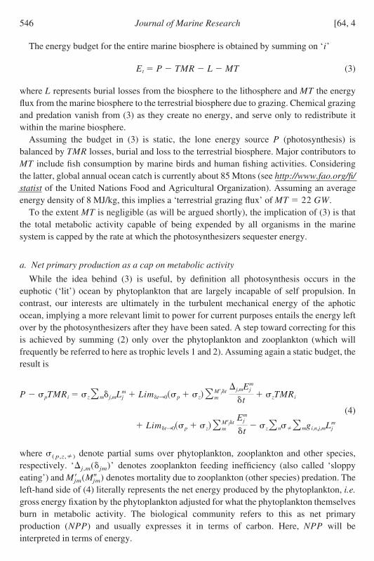
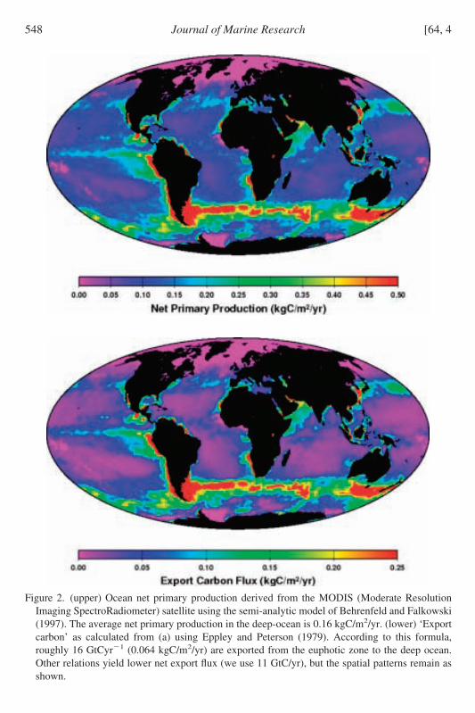
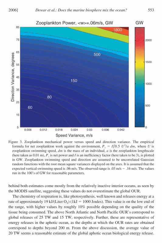
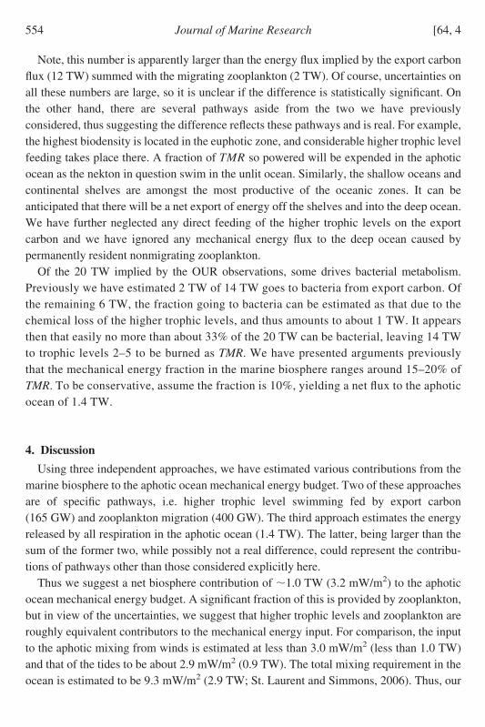
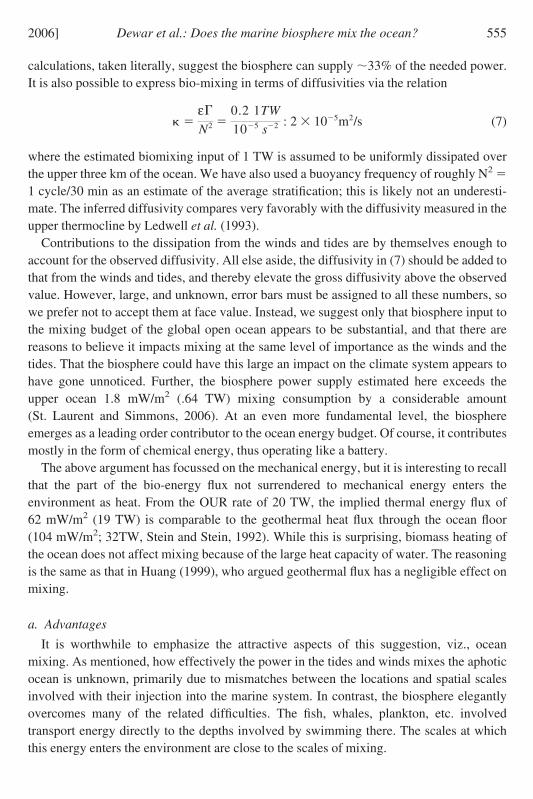
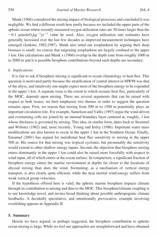
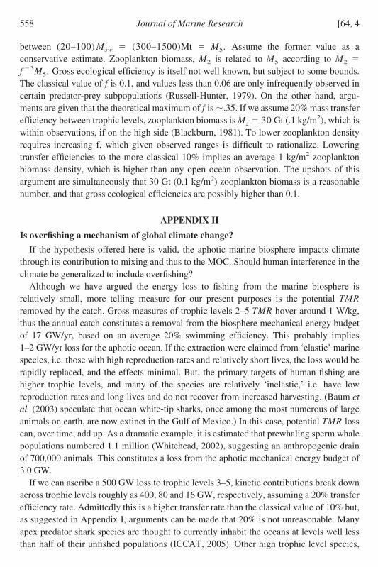
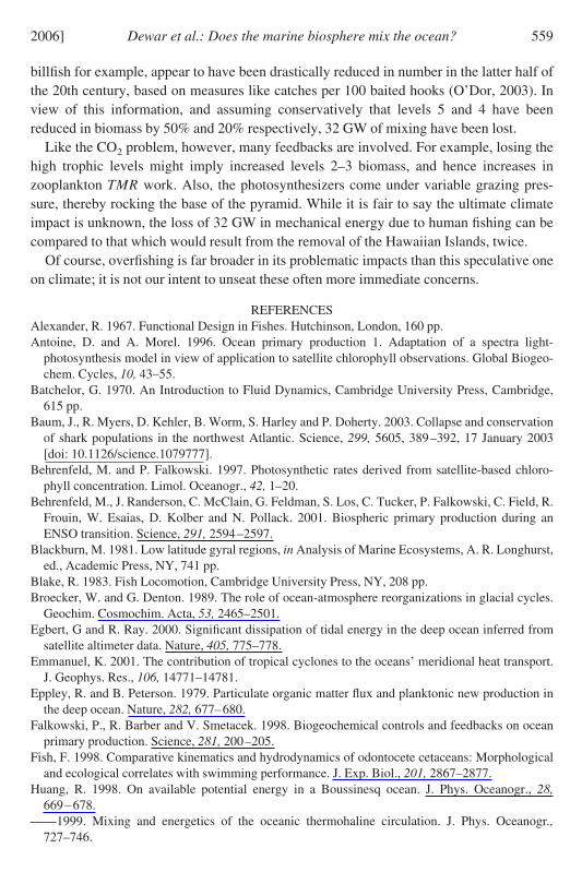
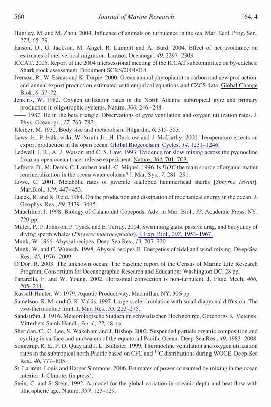