Does the death penalty save lives? - University of Texas ...tvk071000/death_penalty.pdfDoes the death penalty save lives? ... 09008-CrimJournal-Guts.indd 803 10/27/09 7:31 ... rent

803© 2009 American Society of CriminologyCriminology & Public Policy • Volume 8 • Issue 4

Research Article

D e t e r r e n c e a n D e x e c u t I o n s

Does the death penalty save lives?New evidence from state panel data, 1977 to 2006

tomislav V. Kovandziclynne M. VieraitisDenise Paquette bootsU n i v e r s i t y o f T e x a s a t D a l l a s

research summaryEconomists have recently reexamined the “capital punishment deters homicide” thesis using modern econometric methods, with most studies reporting robust deterrent effects. The cur-rent study revisits this controversial question using annual state panel data from 1977 to 2006. Employing well-known econometric procedures for panel data analysis, our results provide no empirical support for the argument that the existence or application of the death penalty deters prospective offenders from committing homicide.

Policy ImplicationsAlthough policymakers and the public can continue to base support for use of the death penalty on retribution, religion, or other justifications, defending its use based solely on its deterrent effect is contrary to the evidence presented here. At a minimum, policymakers should refrain from justifying its use by claiming that it is a deterrent to homicide and should consider less costly, more effective ways of addressing crime.

Keywordsdeath penalty, deterrence, homicide, capital punishment, panel data

The authors would like to thank Gary Kleck, David Greenberg, Paul Zimmerman, Paul rubin, John Donohue, and the anonymous reviewers for their insightful comments and suggestions. Direct correspondence to Tomislav V. Kovandzic, Ph.D., university of Texas at Dallas, 800 West Campbell rd., Gr31, richardson, TX 75080-3021 (e-mail: [email protected]); lynne m. Vieraitis, Ph.D., university of Texas at Dallas, 800 West Campbell rd., Gr31, richardson, TX 75080-3021(e-mail: [email protected]); and Denise Paquette boots, Ph.D., university of Texas at Dallas, 800 West Campbell rd., Gr31, richardson, TX 75080-3021(e-mail: [email protected]).

09008-CrimJournal-Guts.indd 803 10/27/09 7:31:50 PM

Criminology & Public Policy804

There may be people on the other side [of the death penalty debate] that rely on older

papers and studies that use outdated statistical techniques or older data, but all of

the modern economic studies in the past decade have found a deterrent effect.

—Joanna Shepherd, testifying before the Congressional Subcommittee

on Crime, Terrorism, and Homeland Security in 2004

Beginning with the seminal work of Sellin (1959), an extensive body of academic literature has examined the potential deterrent effects of capital punishment on homicide. Sellin’s findings that capital punishment had no discernible deterrent effects on homicide, with

death penalty (DP) states having murder rates equal to or higher than “matched” abolitionist states (see also Dann, 1935; Savitz, 1958), informed death penalty opinion and policy until the controversial work of Isaac Ehrlich emerged in the American Economic Review in 1975. Ehrlich’s more sophisticated methodological analysis suggested that each state-sanctioned execution dur-ing the 1950s and 1960s “saved eight lives.” Moreover, he dismissed the methods employed by Sellin as crude and lacking the necessary scientific rigor to adequately test the complexities of deterrence theory. Ehrlich’s findings were well circulated outside of academic circles, where DP advocates effectively transformed his study into a public policy dictate that “proved” the benefits of continuing executions nationally (Fagan, 2005a).

Ehrlich’s application of more sophisticated econometric techniques to examine the deterrent effects of the DP was a clear advancement over previous work. Despite these improvements, however, Ehrlich’s (1975) study was criticized as suffering from serious empirical infirmities, and as a consequence, its conclusions about the powerful deterrent effects of capital punishment on homicide were later deemed unjustified (Baldus and Cole, 1975; Blumstein, Cohen, and Nagin, 1978; Bowers and Pierce, 1975). Numerous academic papers during the next two decades continued to investigate the potential deterrent effect of capital punishment on homicide, with most criminological studies showing no deterrent effect or even citing a brutalization effect, whereby homicides increased as an unintended consequence of state executions (Cochran and Chamlin, 2000; Lamperti, 2008).

The death penalty debate was ignited once again with the 2003 publication of Dezhbakhsh, Rubin, and Shepherd’s study on the deterrent effect of capital punishment. Using county-level panel data for the post-Gregg era, they estimated that 18 lives were saved each year for each execution. These findings of a strong deterrent effect of the death penalty prompted numerous empirical economists to reexamine the DP efficacy hypothesis using modern econometric meth-ods for panel data, with several studies reporting robust deterrent effects. Yet again, this newest generation of economic deterrence studies has received significant attention from the press, DP advocates, and policymakers who are eager to justify punitive crime-control measures such as the DP (Fagan, 2005b, 2006). Although research conducted by criminologists and some econo-

research Ar t ic le Deter rence and execut ions


805Volume 8 • Issue 4

mists has consistently found little or no support for the deterrent effect of the DP on homicide, empirical economists relying heavily on the Beckerian model of crime have largely ignored or summarily dismissed these studies as lacking appropriate methodological rigor.1 Criminologists and their research are again notably absent from the capital punishment debate.

The current study revisits the controversial question of whether the DP exerts a deter-rent effect on the homicide rate using annual state panel data from 1977 to 2006. This article employs many of the same econometric “bells and whistles” used in recent economic papers on the DP, while substantively contributing to the literature regarding the deterrence hypoth-esis debate as it (1) remedies statistical problems found in several recent DP studies reporting robust deterrent effects; (2) controls for a larger number of potential confounding factors that are theoretically grounded, including several crime policy variables (e.g., three-strikes laws [3X] and right-to-carry concealed handgun laws) and historical events (e.g., U.S. imprisonment binge and crack-cocaine epidemic of the 1980s) that have been linked with cross-temporal changes in homicide rates in the post-moratorium era; and (3) extends the analysis to include additional years (beyond 2000) not covered in recent state panel DP papers. The following section begins with a review of recent economic papers on the DP. We then describe our data and methods and present our results. In the final section, we interpret our results with reference to criminological research on rational choice and offender decision making and consider the policy implications of our findings.

backgroundDuring the last 10 years, an upsurge has occurred in the number of empirical studies, mostly by economists, estimating the average deterrent effect of the DP on homicide rates across states with capital punishment. These studies have primarily relied on annual state- or county-level panel data using fixed-effects models and have operated within the ordinary least-squares (OLS) estimator framework.2 Although some panel research has extended the study period prior to the death penalty moratorium that began with Furman v. Georgia in 1972 (e.g., Dezhbakhsh and Shepherd, 2006; Katz, Levitt, and Shustorovich, 2003), most have focused on within-state (or -county) changes in the overall homicide rates after the reinstatement of capital punishment in Gregg v. Georgia (1976; beginning in 1977 or later). The main differences among the fixed-effects panel studies are the ways in which the authors have conceptualized and operationalized

1. In simple terms, becker’s (1967) principles advance a strongly prorationality position whereby decision making is propelled by cost-driven calculus, such that offenders commit crimes because the potential benefits outweigh the potential risks. It should be noted, however, that other economists have questioned these prodeterrence studies after finding contradictory results and that not all economists endorse beck-erian principles.

2. A few of these studies employ other quasi-experimental designs to analyze the effects of governor- or court-imposed moratoria (e.g., Cloninger and marchesini, 2006) or the extent to which the effects of execution risk are contingent on newspaper publicity surrounding executions (stolzenberg and D’Alessio, 2004). because these studies focus on potential deterrent effects operating in a single DP jurisdiction, as well as for ease of presentation, we did not include them in our review.

Kovandzic , V iera i t i s , boots



execution risk. Given these differences, and for ease of presentation, we organized our review of the latest DP deterrence research based on the measures of execution risk used in each study (i.e., presence of the DP, probability of execution, and frequency of execution). In the next sec-tion, we discuss the methodological shortcomings of studies employing econometric methods for panel data and how these problems are mitigated in the current study.

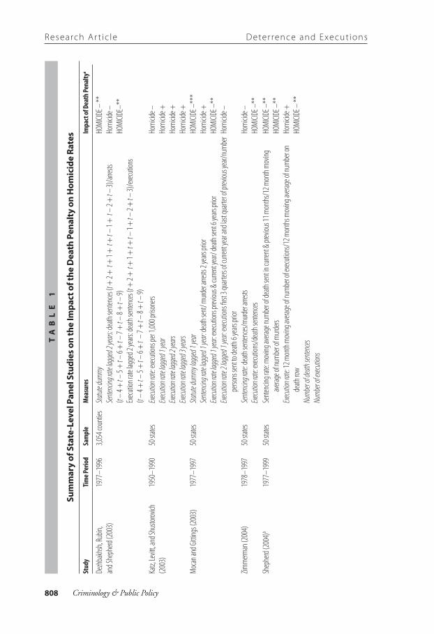
The findings of the latest DP deterrence studies using state- or county-level panel data are summarized in Table 1.3 The table includes the time period covered, unit of analysis, measure used to denote activity status of DP statute or execution risk, and the results obtained for these measures. Comprehensive reviews of the latest DP deterrence studies can also be found in Donohue and Wolfers, (2005), Fagan (2006), Shepherd (2005), and Yang and Lester (2008).

Presence of the Death PenaltyOf the 10 studies published since 2000, 6 examined whether the mere presence (or absence, because of a moratorium or the law being abolished) of the DP was a deterrent to homicide by entering a binary dummy variable into the regression model that took on the value of 1 if the DP was legal in the state and 0 otherwise (Dezhbakhsh et al., 2003; Dezhbakhsh and Shepherd, 2006; Donohue and Wolfers, 2005; Ekelund, Jackson, Ressler, and Tollison, 2006; Mocan and Gittings, 2003; Zimmerman, 2006).4 The dummy variable approach implicitly assumes that the deterrent effects of the DP are unrelated to the probability of execution; rather, the mere existence of capital punishment is assumed to exert a deterrent effect that is not systematically stronger in years with higher actual probabilities of execution.

With the exception of Ekelund et al. (2006), the preponderance of the evidence indicates that the presence of a DP statute was associated with lower homicide rates, although the nega-tive coefficients for the DP dummy variable reported by Donohue and Wolfers (2005) were not significant at conventional significance levels. Specifically, Mocan and Gittings (2003) reported that the presence of the DP reduced the annual number of homicides by 64, whereas Zimmerman (2006) concluded that deterrent effects attributed to the presence of the DP were similar for all five methods of execution. The most notable study to use the dummy variable approach, conducted by Dezhbakhsh and Shepherd (2006), treated the U.S. Supreme Court’s 1972 decision imposing a moratorium on the DP as a “judicial experiment” by coding states a 1 for each year in which the moratorium was in effect and 0 otherwise. In all specifications (see their Table 8), the coefficient on the DP dummy variable was significant and positive, which

indicates that stopping executions increased the homicide rate or that reinstating the DP reduced the homicide rate. Conversely, Ekelund et al. (2006) reported results across specifications that, with a single exception, were statistically significant and positive, which suggests that the pres-ence of an active DP law actually increased homicide during the 1995 to 2000 period.

3. The studies in Table 1 are limited to those published in 2000 or later.

4. Dezhbakhsh and shepherd (2006) switch the coding so that states with an inactive DP law are coded 1 and 0 otherwise.




Probability of ExecutionWith the exception of Dezhbakhsh and Shepherd (2006), all studies listed in Table 1 included some measure of the probability that an offender would be executed. In general, the probability of execution was operationalized as (1) the ratio of the number of executions to the number of homicides (Zimmerman, 2006); (2) the ratio of the number of executions to the number of inmates on death row (Shepherd, 2004); (3) the ratio of the number of executions to the number of offenders sentenced to death (Dezhbakhsh et al., 2003; Mocan and Gittings, 2003; Shepherd, 2005; Zimmerman, 2004); (4) the ratio of the number of executions to the number of prisoners (Donohue and Wolfers, 2005; Katz et al., 2003); and (5) the ratio of the number of executions to population (Donohue and Wolfers, 2005). Again, the main difference occurs in the denominator, where scholars have largely disagreed on the total number of possible outcomes potential murderers are likely to consider when calculating these risks.

Most researchers have used lags ranging from approximately 1 to 6 years in the denomina-tor based on when they expect an execution to impact the homicide rate. The amount of time each variable is lagged depends on the scholar’s estimation of the criminal calculus and/or the processing of an offender through the criminal justice system from arrest to execution. For ex-ample, Mocan and Gittings (2003) and Shepherd (2005) use a 6-year lag in their execution risk measures. The justification for the use of a 6-year lag is based on Bedau’s (1997: 15) estimation that it takes an average of 6 years for an offender to be executed after being sentenced to death (an estimation based on data in the Bureau of Justice Statistics [BJS] report, Capital Punishment, 1994). From a deterrence perspective, potential murderers would conduct a cost–benefit analysis based on the numbers of offenders sentenced to death 6 years before, rather than on current-year sentences. Thus, if offenders are influenced by the probability they will be sentenced and executed, then they would calculate their risk and likelihood based on current-year executions of death row inmates who had been sentenced 6 years earlier.

Other scholars have used a shorter time period under the assumption that offenders will base their decisions on whether to commit homicide on what is currently or recently happened to friends or acquaintances (Donohue and Wolfers, 2005; Shepherd, 2004, 2005). For example, some scholars have defined the probability of execution using current-year death sentences in the denominator of the ratio variable (e.g., Zimmerman, 2004), arguing that prospective mur-derers are unlikely to compute actual probabilities for cohorts of convicted murderers because doing so would be extremely costly for the potential murderer (Shepherd, 2004; Zimmerman, 2004). These scholars have maintained that potential murderers are likely to form expectations based on a “cheaper informational proxy,” such as the current going rate at which convicted murderers are sentenced to death row and executed (Shepherd, 2004: 297).

Regardless of how the probability of execution is measured, studies generally report a nega-tive association between execution risk and the homicide rate, but statistical significance has varied. Katz et al. (2003) reported that the coefficients for the execution rates entered in their regression models were extremely sensitive to model specification and were sometimes positive




ta

bl

e 1

sum

mar

y of

sta

te-l

evel

Pan

el s

tudi

es o

n th

e Im

pact

of t

he D

eath

Pen

alty

on

hom

icid

e ra

tes

Stud

yTim

e Per

iod

Sam

ple

Mea

sure

sIm

pact

of D

eath

Pena

ltya

Dezh

bakh

sh, R

ubin,

an

d She

pherd

(200

3)19

77–1

996

3,054

coun

ties

Statut

e dum

mySe

ntenc

ing ra

te lag

ged 2

years

: dea

th sen

tences

(t +

2 + t

+ 1 +

t +

t – 1

+ t –

2 +

t – 3)

/arres

ts (t –

4 +

t – 5

+ t –

6 +

t – 7

+ t –

8 +

t – 9)

Exec

ution

rate

lagge

d 2 ye

ars: d

eath

senten

ces (t

+ 2 +

t +

1 + t +

t – 1

+ t –

2 +

t – 3)

/exec

ution

s (t –

4 +

t – 5

+ t –

6 +

t – 7

+ t –

8 +

t – 9)

HOMI

CIDE –

**Ho

micid

e –

HOMI

CIDE–

**

Katz,

Levit

t, and

Shus

torov

ich

(200

3)19

50–1

990

50 st

ates

Execu

tion r

ate: e

xecu

tions

per 1

,000 p

rison

ersExe

cutio

n rate

lagg

ed 1

year

Execu

tion r

ate la

gged

2 ye

arsExe

cutio

n rate

lagg

ed 3

years

Homi

cide –

Homi

cide +

Ho

micid

e +Ho

micid

e +Mo

can a

nd Gi

ttings

(200

3)19

77–1

997

50 st

ates

Statut

e dum

my la

gged

1 ye

arSe

ntenc

ing ra

te lag

ged 1

year:

death

sent/

murd

er arr

ests 2

years

prior

Execu

tion r

ate la

gged

1 ye

ar: ex

ecuti

ons p

reviou

s & cu

rrent

year/

death

sent

6 yea

rs pri

or Exe

cutio

n rate

2 lag

ged 1

year:

exec

ution

s first

3 qu

arters

of cu

rrent

year

and l

ast qu

arter

of pre

vious

year/

numb

er pe

rsons

sent

to de

ath 6

years

prior

HOMI

CIDE –

***

Homi

cide +

HO

MICID

E –**

Homi

cide –

Zimme

rman

(200

4)19

78–1

997

50 st

ates

Sente

ncing

rate:

death

sente

nces/

murde

r arre

sts

Execu

tion r

ate: e

xecu

tions

/dea

th sen

tences

Ho

micid

e –HO

MICID

E –**

Shep

herd

(200

4)b

1977

–199

950

state

sSe

ntenc

ing ra

te: m

oving

avera

ge nu

mber

of de

ath se

nt in

curre

nt &

previo

us 11

mon

ths/1

2 mon

th mo

ving

avera

ge of

numb

er of

murde

rsExe

cutio

n rate

: 12 m

onth

movin

g ave

rage o

f num

ber o

f exe

cutio

ns/1

2 mon

ths m

oving

avera

ge of

numb

er on

de

ath ro

wNu

mber

of de

ath se

ntenc

esNu

mber

of exe

cutio

ns

HOMI

CIDE –

**HO

MICID

E –**

Homi

cide +

HOMI

CIDE –

**




Shep

herd

(200

5)19

77–1

996

50 st

ates

Sente

ncing

rate

1: nu

mber

of de

ath se

ntenc

es/nu

mber

of arr

ests fo

r murd

er-2

Sente

ncing

rate

2: nu

mber

of de

ath se

ntenc

es +2

/no o

f arre

sts fo

r murd

erExe

cutio

n rate

1: nu

mber

of ex

ecuti

ons/n

umbe

r of d

eath

senten

ces –

6Exe

cutio

n rate

2: nu

mber

of ex

ecuti

ons +

6/nu

mber

of de

ath se

ntenc

esExe

cutio

n rate

3: ex

ecuti

ons t

+ 2,

t + 1,

t, t –

1, t –

2,

t – 3/

death

sente

nces

t – 4,

t – 5,

t – 6,

t – 7,

t – 8,

t – 9

HOMI

CIDE +

(13 s

tates)

c

HOMI

CIDE –

(6 st

ates)

Homi

cide +

(8 st

ates)

Dono

hue a

nd W

olfers

(200

5)19

60–2

000

1934

–200

019

60–2

000

1978

–199

7

50 st

ates

50 st

ates

50 st

ates

50 st

ates

Statut

e dum

myAc

tive la

w: ≥

1 ex

ecuti

on in

prev

ious d

ecad

eIna

ctive

law: n

o exe

cutio

ns in

prev

ious d

ecad

eExe

cutio

n rate

: exe

cutio

ns/1

,000 p

rison

ersNu

mber

of exe

cutio

nsExe

cutio

n rate

: exe

cutio

ns/1

00,00

0 pop

.Exe

cutio

n rate

2: ex

ecuti

ons/1

,000 p

rison

ersExe

cutio

n rate

3: ex

ecuti

ons/h

omicid

e –1

Execu

tion r

ate: e

xecu

tions

/dea

th sen

t lagg

ed 1

year

Homi

cide –

Homi

cide –

Homi

cide –

Homi

cide +

HOMI

CIDE –

***

Homi

cide –

Homi

cide –

Homi

cide –

Homi

cide +

Dezh

bakh

sh an

d She

pherd

(200

6)19

60–2

000

50 st

ates &

DCNu

mber

of exe

cutio

nsNu

mber

of exe

cutio

ns la

gged

1 ye

arSta

te mo

ratori

um du

mmy

HOMI

CIDE –

***

HOMI

CIDE –

***

HOMI

CIDE +

***

Ekelu

nd, Ja

ckson

, Ress

ler, a

nd

Tollis

on (2

006)

1995

–200

050

state

s & DC

Statut

e dum

myNu

mber

of exe

cutio

ns la

gged

1 ye

arHO

MICID

E+**

*HO

MICID

E– **

*Zim

merm

an (2

006)

1978

–200

050

state

sSta

tute d

ummy

Execu

tion r

ate: e

lectro

cutio

ns/h

omicid

es HO

MICID

E –**

HOMI

CIDE –

**

a Capit

alizat

ion m

eans

the c

oeffic

ient is

signifi

cant.

b Re

sults

repo

rted f

or tot

al ho

micid

e only

. c Sh

ephe

rd tra

nsfor

med t

he st

atisti

cally

signifi

cant

result

s from

all m

odels

into

each

state

’s inc

rease

or de

crease

in th

e num

ber o

f murd

ers af

ter on

e exe

cutio

n. * p =

.10.

**p =

.05.

*** p =

.01.




and sometimes negative. Donohue and Wolfers (2005) generally found no statistically signifi-cant association between execution risk and homicide rates, whereas Dezhbakhsh et al. (2003), Mocan and Gittings (2003), Zimmerman (2004, 2006), and Shepherd (2004) reported robust deterrent effects. In Zimmerman’s (2006) study, however, these effects were significant only for executions by electrocution. None of the other four methods (i.e., lethal gas, lethal injection, hanging, or firing squad) had a significant impact on homicide rates. Finally, Shepherd (2005) found a “threshold effect,” meaning that states that executed more than nine persons during the sample period executions observed lower homicide rates, whereas states that conducted fewer executions had higher homicide rates.

Frequency of ExecutionThe most widely used measure of execution risk in DP deterrence studies has been the frequency of executions (e.g., Dezhbakhsh and Shepherd, 2006; Ekelund et al., 2006; Shepherd, 2004). This conceptualization of deterrence suggests that optimal deterrence is most likely to be realized by simply “reminding” prospective murderers of the state’s willingness to use capital punishment to deter homicide (Kleck, 1979: 896). Thus, regardless of whether prospective murderers are inclined to or capable of calculating the probability of being executed for murder, such persons might still be deterred if increases in executions cause increases in their perceptions of execu-tion risk (presumably through “publicity effects”). Donohue and Wolfers (2005) were critical of the frequency of execution measure because (1) it has the net effect of giving high-execution states, such as Texas and Virginia, greater weight in the homicide regression models and (2) it implies that the effect of an additional execution will vary across DP states depending on the size of the population.5 Dezhbakhsh and Rubin (2007: 17) responded to the criticism levied by Donohue and Wolfers by arguing

an execution in a densely populated state with more crimes, more criminals, and more potential criminals has a stronger deterrent effect, in terms of the number of lives saved, than an execution in a sparsely populated state with few crimes

and few potential criminals. So dividing the number of executions by population makes no sense.

Although the points raised by Donohue and Wolfers call into serious question the theoretical underpinnings used to justify the frequency of executions as a measure of execution risk, we cannot rule it out as one of many possible scenarios through which executions may have the effect of deterring homicide offenders. Indeed, all four studies employing frequency of executions

5. For example, Dezhbakhsh and shepherd (2006) estimate the effect of an execution on the homicide rate to be –0.145, which implies that each execution in Texas reduces the annual number of homicides by roughly 20, whereas in Delaware, it reduces the annual number of homicides by almost 1.




as a measure of execution risk found strong support for the DP deterrence-efficacy hypothesis. These results suggest that executions might exert a unique deterrent effect on homicide rates even in years when the actual probability of execution for murder in the same state is less than in previous years or greater than in other DP states (Dezhbakhsh and Shepherd, 2006; Donohue and Wolfers, 2005; Ekelund et al., 2006; Shepherd, 2004).

In sum, although most scholars studying the deterrent effects of the DP have agreed that deterrence depends more heavily on the actual risk of execution rather than on the mere exis-tence of the DP (e.g., Dezhbakhsh and Rubin, 2007; Mocan and Gittings, 2003), they have differed on which factors prospective murderers consider when calculating such risks. Given the lack of reliable information on how prospective murderers assess the risk of execution, if at all, it is not surprising that there is no theoretical or empirical consensus on how best to measure execution risk. More importantly, however, DP scholars have necessarily assumed that any such measure of actual execution risk would have a positive effect on average perceptions of execution risk among prospective murderers. Research by Kleck, Sever, Li, and Gertz (2005) suggests, however, that the perceived risk of punishment has little or no relationship to the actual risk of punishment, and this finding may apply specifically to the risk of execution.

Data and statistical MethodsSimilar to recent economic papers on capital punishment, we reexamine the “DP deters homi-cide thesis” using annual, state panel data. Because we are solely interested in assessing potential deterrent effects of capital punishment in the post-Gregg era, we begin our study period in 1977 but extend the study period used in recent studies from 2000 to 2006.6 The primary advantage of the panel design, as opposed to the more commonly used time-series design (e.g., national time-series studies) in earlier DP deterrence research, is that it provides a comparison group by treating non-DP states as a control group for DP states (Campbell and Stanley, 1963). We are not, however, asserting that non-DP states represent a control group in the strict sense of the term, as this would imply the DP is a “natural experiment.” The defining feature of a true natural experiment is that assignment of treatment conditions occur in an “as if” random fash-ion (Dunning, 2005). Because it is unlikely that the decision to enact, abolish, halt, or apply the DP in the post-Gregg era occurs independently of other sociopolitical forces operating in DP states, we do not believe a credible claim can be made that DP and non-DP states are “as if” randomly assigned. As a result, we do not assume “pretreatment” equivalence between DP and non-DP states; rather, we follow the standard solution in nonexperimental research (and recent DP deterrence papers) of measuring and statistically controlling for as many potential confounding factors—that is, correlates of the presence of the DP and risk of execution that could influence homicide rates—as possible. We also follow common practice in state panel studies of the DP (and crime-control initiatives in general) by including state fixed effects, year fixed effects, and state-specific time trends in the homicide specifications to minimize potential

6. None of the latest DP panel studies of which we are aware uses data that extends past 2000 (see Table 1).




endogeneity problems related to omitted variable bias. A detailed discussion of how these proxy variables minimize the effects of omitted variable bias is provided in the next section.

Death Penalty MeasuresAs discussed, deterrence theory provides multiple pathways by which the DP could serve as a deterrent to potential murderers. Given the nature of the study and the lack of a general con-sensus on how prospective murderers might form these expectations (assuming they will do so at all), we felt it was important to include all of them in the current study. The measures used to capture both the presence of the death penalty and execution risk are as follows:

Death Penalty Law Status Variables:DP law dummy variable (year 1. t)DP law dummy variable (year 2. t – 1)

Frequency of Executions:Number of executions (year 3. t)Number of executions (year 4. t – 1)

Probability of Execution Measures:Executions (year 5. t) per 1,000 prisoners (year t)Executions (year 6. t)/death sentences (year t – 1)Executions (year 7. t)/death sentences (year t – 6)Executions (year 8. t) per 100,000 state population (year t)Executions (year 9. t)/homicides (year t – 1)

Data regarding the legal status of the DP through 2000 were obtained from Dezhbakhsh and Shepherd (2006: 513). Using sources cited in Dezhbakhsh and Shepherd, we collected ad-ditional information on the legal status of the DP through 2006. Year-end data on the number of prisoners currently on death row; those receiving a death sentence or executed in the current year; or those persons removed from death row because of a sentence vacation/commutation, death from natural causes, suicide, escape, or drug overdose from 1977 to 2005, came from “Capital Punishment in the United States, 1973–2005” (Bureau of Justice Statistics, 2005).




Year-end statistical tables and data from 2006 were downloaded from the Bureau of Justice Statistics (2007) Web site as well.7

Homicide RatesIt has been suggested by some that, because the DP can only be applied to capital murders, the most appropriate dependent variable in a DP deterrence study is the rate of capital murders (e.g., Bailey, 1983; Fagan, Zimring, and Geller, 2006; Peterson and Bailey, 1991; Sellin, 1959; Van den Haag, 1969). We maintain that an equally valid argument can be made for the use of the total homicide rate to test the DP efficacy hypothesis. Drawing on Van den Haag’s (1969) conceptualization of deterrence, Kleck (1979) argued that the deterrent effects of the DP need not be limited to prospective offenders engaging consciously in risk–benefit calculations but to all homicides, as “the cognitive link in potential offenders’ minds may be between the ultimate legal sanction, death, and the act of homicide rather than any particular arbitrary legal subtype of homicide.” (1979: 890). Kleck’s application of Van den Haag’s preconscious deterrence theory to the DP provides a theoretical rationale for broadening the search for potential deterrent ef-fects by including both death and non-death-eligible homicides in the homicide rate measure (see Shepherd, 2004, for empirical support).

Homicide data were obtained from the Federal Bureau of Investigation’s (FBI’s) Uniform Crime Reporting (UCR) Program, published as Crime in the United States. UCR homicide data from 1977 to 2006 are available on-line at the BJS Web site (ojp.usdoj.gov/bjs/dtd.htm). We rely on the FBI’s UCR homicide measure—as opposed to homicide data based on death certificates collected as part of the National Vital Statistics System by the National Center for Health Statistics (NCHS)—because the latter are available only through 2005.8

7. Analyses that measure execution risk based on the number of death sentences issued in the previous year or 6 years prior cover the period 1978 to 2006 and 1984 to 2006, respectively. The rationale for excluding earlier years was that few criminals were sentenced to death during the 4-year hiatus (1972–1976) on capital punishment after the Furman v. Georgia (1972) decision. As a result, measures of execution risk calculated using death sentences meted out during the years of the ban would be undefined (because of the zero denominators), and it is impossible to know how prospective murderers during the years 1978 to 1982, for example (assuming death sentences meted out in the previous 6 years is the correct denomi-nator), would have calculated their risk of execution. even after excluding these years, the measures of execution risk remained undefined in many instances because no death sentences were issued by the state in the previous year (or 6 years earlier). To avoid losing these state/years in the analysis, undefined observations were assigned a score of 0. Coefficient estimates for the ratio variables were qualitatively similar when treating undefined observations as missing data.

8. After the data analysis was completed, we obtained homicide data based on death certificate data for 2006 using the Centers for Disease Control and Prevention’s WIsQArs interactive database system. Although not shown, the sign and size of the coefficients obtained for the execution risk measures were largely similar when substituting the FbI’s uCr homicide measure for the NCHs homicide measure.




Specific Control VariablesCrime policy initiatives and the crack epidemic. As discussed, most of the latest DP papers failed to account for other important crime-control initiatives or important historical events that occurred in the post-moratorium era. The passage of “three strikes and you’re out laws,” for example, have been linked with homicide increases (Kovandzic, Sloan, and Vieraitis, 2002; Marvell and Moody, 2001) and decreases (Shepherd, 2002).9 In addition, a large number of academic studies have examined the potential deterrent impact of right-to-carry concealed handgun (RTC) laws on homicide rates, with mixed results. Although Lott and Mustard (1997) and Lott (2000) reported robust evidence of deterrence, several researchers who reanalyzed (and extended) their data (e.g., Ayres and Donohue, 2003, 2009a, 2009b) concluded that “the statisti-cal evidence that these [RTC laws] have reduced crime is limited, sporadic, and extraordinarily fragile” (Ayres and Donohue, 2003: 1201). In any event, several published studies support the RTC law-efficacy hypothesis, and we err on the side of caution by including an RTC law vari-able as a regressor to avoid a potential model underfitting problem. Both laws are represented with a binary dummy variable scored “1” starting the full first year after a law went into effect and “0” otherwise. Dates for the passage of 3X laws were obtained from Marvell and Moody (2001). Dates of passage for RTC laws were obtained through statutory research conducted by Marvell (2001) and the senior author.

We also control for the prevalence of crack cocaine using an index created by Fryer, Heaton, Levitt, and Murphy (2005). The crack index is composed of various indirect proxies of crack prevalence, including cocaine arrests, cocaine-related emergency room visits, cocaine-induced drug deaths, crack mentions in newspapers, and Drug Enforcement Administration drug busts. Unfortunately, the crack index variable is only available through 2000. Rather than shorten the study period by 6 years, we only enter the crack index variable in separate estimations when examining the robustness of the baseline homicide specifications. Data for the crack prevalence measure were obtained from Roland Fryer’s Web site at post.economics.harvard.edu/faculty/fryer/fryer/.html.

Socioeconomic control variables. Socioeconomic variables included in the homicide specifi-cations are those commonly used in recent DP papers and in macrolevel studies of homicide in general. Specifically, we control for the percent of the civilian labor force unemployed; the total employment rate; real per-capita income (divided by the Consumer Price Index); percent of the population living below the poverty line; percent of the population residing in metropolitan areas; percent of the population with a bachelor’s degree or higher; per-capita beer consumption (measured in gallons); and the percent of the population ages 15 to 24, 25 to 34, and 35 to 44 years. Poverty data were obtained from the Bureau of the Census Web site at census.gov/hhes/www/poverty. The data on state-level unemployment were taken from the Bureau of Labor

9. between 1993 and 1996, 25 states and the federal government enacted 3X laws (Austin and Irwin, 2001). studies that found a positive association between 3X laws and homicide speculate that felons who face lengthy prison terms after conviction for a third strike may decide to kill victims, witnesses, or police of-ficers during an attack that would otherwise be nonlethal to reduce the chance of apprehension.




Statistics Web site at bls.gov/sae/home. Data on personal income and real welfare payments were obtained from the Bureau of Economic Analysis Web site at bea.doc.gov/bea/regional/reis/. The percent of the population with college degrees or higher and residing in metropolitan areas are linear interpolations of decennial census data, as reported in various editions of the Statistical Abstracts of the United States. Data on beer consumption were obtained from the Beer Institute Web site at beerinstitute.org. The age group data were obtained directly from the U.S. Bureau of the Census on computer disk.

Deterrence measures. Deterrence measures include the number of police officers per 100,000 population, the state incarceration rate (again, per 100,000 population), and the prison death rate.10 The latter measure is used to proxy for the quality of life in prisons, which Katz et al. (2003) argued and demonstrated to be a deterrent to criminals. The variable is defined as the number of prisoners who die in prison from all sources (except executions) per 1,000 state prisoners. The data on the total number of police (including civilians) were from the Public Employment series prepared by the Bureau of the Census. The data on the number of prisoners (sentenced to prison more than a year in custody as of December 31) were obtained directly from the BJS Web site at ojp.usdoj.gov/bjs. Prison death data from 1977 to 2000 were obtained from Justin Wolfers’ personal Web site at bpp.wharton.upenn.edu/jwolfers/DeathPenalty.shtml. The data from 2001 to 2006 were obtained from the BJS’s “Deaths in Custody Reporting Program” (Bureau of Justice Statistics, 2008).

Statistical Methods for Panel DataWe follow conventional strategies for panel studies of crime and estimate a fixed-effects model. The fixed-effects model requires adding a dummy variable for each state and year (except the first to avoid dummy variable trap). The state (cross-sectional) fixed effects control for time-invariant unobserved factors that influence homicide rates in a particular state.11 The year fixed

10. The data are for the end of the year, and we estimate the prison population during the year by averaging the current and prior year numbers. We follow the conventional practice of lagging the police and prison measures by 1 year to mitigate potential simultaneity bias.

11. The Hausman specification tests strongly rejected the notion of no systematic differences between the fixed-effects and random-effects models.




effects control for unobserved factors that are common to all states in a particular year.12 Because the analysis includes both state and year fixed effects, the parameter estimates for all explana-tory variables are based solely on within-state variation. We also control for state-specific time trends by including a separate linear trend variable for each state. The inclusion of state-specific time trends has become standard practice in panel studies of crime (e.g., Ayres and Donohue, 2003; Donohue and Wolfers, 2005; Marvell and Moody, 1996; Mocan and Gittings, 2003). The state-specific linear time trends control for unobserved, slow-moving, sociodemographic factors that affect the time-series behavior of the homicide rate in each state and differ from the nationwide trends captured by the year fixed effects.

The next issue for the homicide rate model regards choice of functional form. The most common practice in the recent DP literature and the procedure followed here is to assume a linear functional relationship between the risk of execution and homicide rates. Although the preference in state panel studies of crime is to use a log-log model, this would force us to address the problem of having a large number of 0-valued observations for the execution risk measures that cannot be logged. It is common to add some small amount (usually a 1) to 0 values so that a logarithmic functional form may be used. However, this procedure is inappropriate where, as here, there are a large number of 0s (Wooldridge, 2005: 185). Because we have no strong theo-retical basis for choosing one functional form over another, we also present alternative estimates using a log-level model in which only the dependent variable (i.e., the homicide rate) is logged. The log-level model is intuitively appealing, especially for those who champion the economic model of crime, because it implies that as execution risk increases, the deterrent effects of the DP on the homicide rate will accelerate.

We also follow recent convention in panel data analysis of assuming “clustered errors” and compute heteroskedasticity-autocorrelation robust standard errors clustered at the state level. The benefit of using cluster robust standard errors is that they allow for general forms of heteroskedasticity as well as for arbitrary serial correlation within a given state (Wooldridge, 2001). Failing to account for the presence of clustered errors produces biased estimates of

standard errors and overstated estimated significance levels. We also report estimates using heteroskedasticity-robust standard errors but adopt another widely popular approach in panel

12. We used an F test to determine whether, as a group, the year dummies affected cross-temporal changes in homicide rates. Not surprisingly, the F statistic shows the year dummies are jointly statistically significant at the .01 significance level. Interestingly, Dezhbakhsh and shepherd (2006) chose not to include year fixed effects in their homicide specifications, although their importance in minimizing omitted variable bias is well documented in the crime literature using the panel data approach. In fact, we are not aware of any published panel studies of crime that have tested (using an F test) and not found the year dummies to be highly significant as a group. Instead, the authors opted for the use of decade fixed-effects that control for the average homicide rate in each decade. The problem with this approach, however, is that it fails to take into account the fact that trends in homicide rates have varied largely within each decade since the 1960s (see also Donohue and Wolfers, 2005: 805–806). Not surprisingly, when Donohue and Wolfers (2005) reestimated Dezhbakhsh and shepherd’s specification examining the impact of state DP moratoriums (imposed by the 1972 supreme Court decision in Furman v. Georgia) on homicide rates (see their Table 8, Column 2) while controlling for year fixed effects, the coefficient on the DP moratorium dummy variable was cut almost in half and no longer statistically significant.




studies, which is to enter a 1-year lag of the dependent variable in the specification to correct for serial correlation and to mitigate omitted variable bias (Beck and Katz, 1995, 1996). As is well known, per-capita variation in crime rates is greater in low-population states. In this case, the OLS estimator is no longer efficient. In an attempt to gain efficiency in our parameter estimates, we decided to use weighted least squares (WLS) regression, where the weights are the number of people who live in each state. Although population size may not correspond to the inverse of the error variances, the WLS estimator is likely to be more efficient than OLS. Importantly, even if the weights are not optimal or heteroskedasticity remains, the use of robust standard errors (clustered or not) will still provide for robust inference.

t a b l e 2

summary statistics

Overall Within– Mean SD State SD

Dependent variablesHomicides per 100K 6.290 3.572 1.680

Death penalty variablesDeath penalty dummy variable 0.719 0.450 0.172Executions(t) .703 2.803 2.096Executions(t) per 1,000 prisoners(t) .030 .094 .085Executions(t)/death sentences (t–1) .092 .320 .283Executions(t)/death sentences(t–6) .102 .348 .311Executions(t) per 100K(t) .012 .038 .033Executions(t)/homicides(t–1) .002 .008 .007

Policy control variableRight-to-carry concealed law dummy variable .230 .416 .3383X law dummy variable .193 .391 .335

Sociodemographic control variablesUnemployment rate 5.878 2.004 1.659Employment rate 55,631.03 6,026.39 4333.71Poverty rate 12.841 3.937 2.020Real per-capita income 4.777 .920 .631Percent persons ages 15 to 24 15.660 2.131 1.986Percent persons ages 25 to 34 15.565 1.987 1.711Percent persons ages 35 to 44 14.275 2.053 1.886Beer shipments (31-gallon barrels) per 100K 75,303.87 13,108.02 5,442.83Percent persons with college degree 20.954 5.497 4.165Percent persons residing in metropolitan areas 65.887 21.322 3.249Crack index, 1980 to 2000 0.948 1.264 1.075

Deterrence variablesPrison deaths per 1,000 prisoners 128.504 155.616 72.785Prisoners per 100K 257.066 149.761 113.874Police officers per 100K 265.764 50.188 24.278

Notes. Descriptive statistics are for the 1977 to 2006 time period except where noted in text. Means and standard deviations are unweighted. The data sources are described in the text.




Next, we examined the stationarity of the homicide rate using the panel unit root test advocated by Im, Pesaran, and Shin (2003), hereafter indicated by IPS. Assessing the stationar-ity of homicide is important, as standard significance tests assume variables have the property that the mean and variance are constant over time (Moody, 2005). The IPS test is based on the null hypothesis that all homicide series are generated by unit-root processes. The alternative is that at least one homicide series is stationary. For panel unit-root tests, the lag length has to be chosen. The data are annual, so a lag length of 1 was chosen, but similar results were obtained when using lag lengths of 2 and 3 years. The results of the IPS test reject the null hypothesis of a unit root in homicide rates at the 1% level. The standardized t-bar statistics for the homicide rate are –4.21 (p < .000), –2.814 (p < .002), and –2.975 (p < .001) when the lag lengths are set equal to 1, 2, and 3 years, respectively. These results both replicate the mean-reverting property of the homicide rate reported by Moody (2005) and show that his results do not change with extended data. Because homicide seems to be a stationary process, there is no need to first-difference the variables (i.e., we estimate the regressions using levels of variables).

Finally, an examination of collinearity diagnostics reveals no serious collinearity problems for any of the DP measures, although it does affect some of the other explanatory variables. This occurs mainly for the socioeconomic variables that change slowly over time and are highly correlated with the state fixed effects. Thus, it is necessary to use caution in the interpretation of results for these slow-moving variables.

Table 2 lists the variables used in the regression models. In addition to the variable name and a brief description, the mean, and overall and within-state standard deviations are shown. Estimation was carried out in Stata, version 9.0 (StataCorp., College Station, TX).

empirical resultsTable 3 presents the results of eight separate homicide estimations using regression procedures for panel data discussed in the previous section. The most notable features include using state and year fixed effects and linear state-specific time trends, and using WLS, where the weight is the state’s share of the U.S. population. Heteroskedasticity-autocorrelation robust standard errors, which are clustered at the state level, are presented in parentheses under the regression coefficients. Each homicide model includes, one at a time, a measure that captures the pres-ence of a DP statute, the frequency of executions, or the probability of execution for homicide. Because of space limitations, the regression coefficients for the state and year fixed effects and linear state-specific time trends are not shown.

Presence of the Death Penalty and HomicideWe begin the analysis by examining whether a baseline deterrent effect of the DP on homicide rates is attributable to the presence of an active DP statute. Because our study sample begins in the post-moratorium era, we cannot assess the effects on homicide rates of state DP statutes reenacted after the Furman v. Georgia (1972) decision (which became effective after the U.S. Supreme Court’s decision on July 2, 1976) or those state statutes enacted during the year 1977




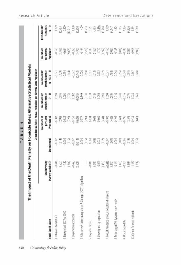
(e.g., CA, NC, and WY). Any deterrent impact caused by the presence of these laws is captured by the state fixed-effects variables. Nevertheless, we still can assess the effects of 11 separate changes to state DP statutes that have taken place from 1977 to 2006. Of these 11 policy changes, 8 were based on states enacting (in some cases, reenacting) a DP law (KS, 1994; MA, 1982; NH, 1991; NJ, 1982; NM, 1979; NY, 1995; OR, 1978; SD, 1979), 1 abolishing its DP statute (RI, 1984), and 2 suspending executions because of a Governor-ordered moratorium (IL, 2000; MD, 2002).13 Similar to Donohue and Wolfers (2006), we use a binary dummy variable set equal to 1 when a state has an active DP statute and 0 otherwise.

t a b l e 3

the Impact of the Death Penalty on homicide rates: estimates from state Panel Data, 1977 to 2006

Dependent Variable: Annual Homicides per 100,000 State PopulationVariable (1) (2) (3) (4) (5) (6) (7) (8)

Death penalty dummy variable (t) –0.416 (.507) Executions (t) — –0.007 — — — — — — (.014) Executions (t–1) — — 0.006 — — — — — (.008) Executions (t) per 1,000 prisoners (t) — — — –0.102 — — — — (.593) Executions (t)/death sentences (t – 1) — — — — 0.094 — — — (.087) Executions (t)/death sentences (t – 6), (t – 1) — — — — — –0.071 — — (.129) Executions (t) per 100K (t) — — — — — — –0.166 — (1.399) Executions (t)/homicides (t – 1) — — — — — — — 1.799 (5.763)Prison death rate 0.001 0.002 0.002 0.002 0.001 0.0002 0.002 0.002 (.001) (.001) (.001) (.001) (.001) (.002) (.001) (.001)

13. massachusetts abolished its DP in 1984, whereas the New York state supreme Court ruled the state’s DP law unconstitutional in June 2004. rather than estimate separate effects for both the enactment and the abolition of these state laws, we follow the strategy of Dezhbakhsh and shepherd (2006) and create a single law dummy variable that accounts for both policy changes simultaneously. For example, the DP law dummy variable for New York is coded 0 for the years 1977 to 1994, 1 for the years 1995 to 2003, and 0 for the years 2004 to 2006.




Shall issue law –0.345 –0.317 –0.332 –0.324 –0.338 –0.413 –0.323 –0.328 (.260) (.263) (.259) (.258) (.268) (.270) (.259) (.259)3X law 1.044 1.085 1.101 1.093 1.097 1.038 1.092 1.097 (.500) (.572) (.569) (.570) (.567) (.620) (.571) (.57)Unemployment rate –0.124 –0.112 –0.116 –0.113 –0.104 –0.041 –0.114 –0.115 (.061) (.062) (.063) (.060) (.069) (.099) (.061) (.062)Employment rate × 100 0.003 0.004 0.004 0.004 0.002 –0.004 0.004 0.004 (.007) (.007) (.007) (.007) (.008) (.010) (.007) (.007)Poverty rate 0.040 0.040 0.040 0.040 0.033 0.010 0.040 0.040 (.040) (.040) (.041) (.040) (.041) (.042) (.040) (.040)Per-capita income 0.168 0.160 0.178 0.163 0.236 0.004 0.165 0.177 (.718) (.716) (.718) (.721) (.734) (.764) (.716) (.717)Percent aged 15 to 24 0.118 0.105 0.105 0.105 0.221 0.612 0.105 0.105 (.196) (.190) (.191) (.191) (.180) (.215) (.191) (.190)Percent aged 25 to 34 0.397 0.366 0.369 0.368 0.423 0.812 0.368 0.367 (.255) (.249) (.248) (.248) (.239) (.310) (.248) (.248)Percent aged 35 to 44 –0.105 –0.111 –0.114 –0.113 –0.062 –0.026 –0.113 –0.114 (.236) (.231) (.233) (.231) (.246) (.329) (.232) (.233)Prisoners per 100K, (t – 1) –0.009 –0.009 –0.009 –0.009 –0.008 –0.009 –0.009 –0.009 (.002) (.002) (.002) (.002) (.002) (.002) (.002) (.002)Police officers per 100K, (t – 1) –0.011 –0.012 –0.012 –0.012 –0.013 –0.017 –0.012 –0.012 (.005) (.006) (.006) (.006) (.006) (.007) (.006) (.006)Beer consumption × 100 0.004 0.004 0.004 0.004 0.002 0.008 0.004 0.004 (.003) (.003) (.003) (.003) (.003) (.004) (.003) (.003)Percent college degree 0.254 0.251 0.257 0.254 0.174 0.290 0.253 0.255 (.170) (.175) (.175) (.174) (.172) (.293) (.174) (.174)Percent metropolitan –0.023 –0.021 –0.022 –0.021 –0.013 –0.051 –0.022 –0.022 (.043) (.042) (.042) (.042) (.048) (.090) (.042) (.042)Sample size 1,499 1,499 1,499 1,499 1,449 1,149 1,499 1,499Adjusted R2 .94 .94 .94 .94 .94 .93 .94 .94

Notes. The dependent variable is the annual number of homicides per 100,000 state population. The study period is 1977 to 2006 except as noted in the text. Prison death data for Alaska in 1994 are missing. The regressions are weighted by state population. Although not shown, state fixed effects, year fixed effects, and state-specific linear trends are included in all estimations and are always significant as a group using an F test. Heteroskedasticity and autocorrelation robust standard errors are reported. Coefficients that are significant at the 10% level are underlined. Coefficients that are significant at the 5% level are in bold. Coefficients that are significant at the 1% level are in bold and underlined.

The results for the DP law dummy variable are presented in column 1. Contrary to the findings reported by Dezhbakhsh and Shepherd (2006) and Mocan and Gittings (2003), but consistent with those reported by Donohue and Wolfers (2005), our results indicate no relation-ship between the activity status of the DP and homicide. Although the coefficient on the DP law dummy variable is in the negative direction, which is consistent with the DP deterrence hypothesis, it is not significantly different from 0. Next, we reestimated the specification in column 1 but lagged the DP law dummy 1 year to account for potential delays in the diffusion of information about a DP regime and, thus, its ability to alter prospective murderers’ aware-ness of the possibility of being executed for murder. Lagging the DP law dummy variable by




1 year also helps to mitigate potential simultaneity bias if increases in the homicide rate lead state policy makers to adopt DP legislation. Although not shown, the coefficient on the DP law dummy was even smaller in absolute value than the current-year value and remained statisti-cally insignificant. In all, the results of the dummy variable analysis provide little systematic evidence that the mere possibility of being executed for murder serves as an effective deterrent to potential murderers, at least not during the post-moratorium era.

Admittedly, one drawback to this analysis is that most states with currently active DP statutes (re)enacted them prior to 1977. As a result, we only could assess the potential deterrent impact of the presence of the DP on homicide in a minority of DP states. Perhaps more importantly, the dummy variable approach cannot address what most DP deterrence scholars consider to be the more relevant empirical question related to the DP deterrence hypothesis: Do higher levels of execution risk produce stronger deterrent effects? As discussed, most DP scholars argue that the strongest deterrent effects of the DP are likely to be linked to its application in practice. For example, if the cognitive link in a potential murderer’s mind is the actual risk of execution for homicide, rather than the possibility of execution, then the appropriate independent vari-able in a DP study is the frequency of executions or the probability of execution for homicide rather than its presence. Indeed, most of the DP papers reviewed in Table 1 find the strongest support for the DP-deters-homicide hypothesis when examining the link among the frequency of executions (e.g., Dezhbakhsh and Shepherd, 2006), probability of execution (e.g., Mocan and Gittings, 2003), and homicide rates rather than the legal status of the law. As a result, we turn our attention on the relationship between the application of the DP and homicide using measures most commonly employed in recent DP deterrence research.

Number of Executions, Probability of Execution, and HomicideColumns 2 through 8 report the results of seven different estimations using the same exact model specification employed in Column 1 but replace the DP law dummy variable with either the frequency of executions or the probability of execution for a given cohort of incarcerated murder-

ers. Again, we emphasize that what is important from a deterrence perspective is a prospective murderer’s perceived risk of execution for homicide. Obviously, direct measures of perceived risk of execution at the aggregate level are nonexistent, and thus, DP scholars have been forced to use aggregate-level measures of actual execution risk as proxies for the aggregate perceived risks. To the extent that aggregate-level measures of actual execution risk have a significant positive association with the perceived risks, the objective risks should provide a satisfactory proxy for the perceived risks (but see Kleck et al., 2005).

The results in Column 2 are based on Dezhbakhsh and Shepherd’s (2006) preferred measure of simply using the total number of executions in a state–year. Contrary to the findings reported by Dezhbakhsh and Shepherd (2006), our results indicate that increasing the scale of executions does not lead to greater deterrent effects by “sending a message” to potential murderers of the state’s willingness to execute persons convicted of homicide. The sign on the execution variable




is negative but far from significant. Importantly, the coefficient on the execution measure is roughly one twentieth the size reported by Dezhbakhsh and Shepherd (2006; see their Table 8, Column 1). Lagging the execution variable 1 year to account for potential delays in the transmis-sion of this deterrence message produced substantively similar results (Column 3). Needless to say, the vastly different results obtained by Dezhbakhsh and Shepherd (2006) and the current study for the execution measure was a source of concern for us. As one of our many robustness checks, we altered our baseline specification to resemble more closely the estimation method used by the authors to identify the source of the differences. We believe the results obtained by Dezhbakhsh and Shepherd (2006) for the execution measure were a by-product of omitted variable bias and failing to adjust standard errors for the presence of serial correlation.

Column 4 reports estimates using executions carried out in year t per 1,000 state prisoners as recommended by Katz et al. (2003). Interestingly, the sign and value of the coefficient for the execution variable are identical to those reported by Katz et al. (2003; see their Table 2, Column 6), although we report standard errors much larger than theirs. Regardless, our finding of no significant relationship between the risk of execution and the homicide rate is consistent with that reported by Katz et al. (2003). Columns 5 and 6 report estimates using slightly different variants of ratio variables capturing the actual objective probability of execution for homicide. The first ratio measure is similar to the one used by Zimmerman (2004) and is the number of executions carried out in year t divided by the number of persons sentenced to death row in year t – 1. The second ratio measure, which was employed by Mocan and Gittings (2003), is similar to the first measure except that the denominator is death sentences in year t – 6.14 The theoretical justification for lagging the denominator by 1 and 6 years was discussed above. In both cases, the coefficients on the execution risk measures are far from significant and in the case of the former measure it is actually in the unexpected positive direction.15 We also created risk of execution measures assuming the average wait on death row was 4 and 5 years. Although not shown, the results for these alternative versions were largely similar to those obtained when deflating the denominator by 6 years.

The last two execution measures in Table 3 were employed exclusively by Donohue and Wolfers (2005). Column 7 reports estimates using executions in year t per 100,000 population,

whereas the results in Column 8 are based on estimations using executions divided by homicide in year t – 1.16 Once again, these execution risk measures fail to reveal any significant negative relationship between the risk of execution and homicide. The coefficients for both execution

14. Following mocan and Gittings (2003), we lag the risk of execution measure by 1 year to be more consis-tent with their specification.

15. Donohue and Wolfers (2005) employ a slightly different variant of Zimmerman’s execution measure in which they lag the numerator by 1 year to mitigate simultaneity bias. We also tried this measure, and it produced results largely similar to those obtained using the Zimmerman measure.

16. Donohue and Wolfers (2005) use executions per 100,000 population because of the scaling problems discussed earlier when using only the sheer number of executions.




risk measures are far from significant, and the sign on the latter measure is in the unexpected positive direction.

Other Notable FindingsAlthough it is not the focus of the current study, the performance of the specific control variables in Table 3 are worth a brief mention because many of them are considered important correlates of homicide, and the results for these explanatory variables may, at least for some readers, speak volumes with regard to the reliability of the findings for the DP deterrence measures. First, we find no evidence that increases in the presence of young adults is associated with higher rates of homicide. These results support recent empirical works by Levitt (1999) and Marvell and Moody (2001). With respect to the policy variables, the adoption of 3X laws is positively cor-related with higher homicide rates. This finding is consistent with Kovandzic et al. (2002) and Marvell and Moody (2001). Similar to Ayres and Donohue (2003) and Kovandzic, Marvell, and Vieraitis (2005), we find no evidence to support a deterrent effect of the passage of shall-issue concealed handgun laws. We also find no evidence that worsening prison conditions, as proxied by prison deaths, reduces the homicide rate. These results parallel those reported by Katz et al. (2003), although the authors reported statistically significant decreases in almost all cases for the violent crime rate and in a few cases for the property crime rate. Last, police levels and prison population growth are both significantly related to lower homicide rates. This finding largely mirrors those reported in other state panel studies (e.g., Katz et al., 2003; Levitt, 1996; Marvell and Moody, 1994, 1996; Zimmerman, 2004).

Does a Two-Way Relationship Exist Between Execution Risk and Homicide?Recent DP deterrence authors (e.g., Mocan and Gittings, 2003; Zimmerman, 2004) have suggested that coefficients for execution risk measures might suffer from simultaneity bias if increases in homicide rates heighten public fear of crime and, in turn, encourage prosecutors to seek the DP more often and make judges less likely to overturn death sentences imposed by juries. Research also suggests that public opinion and elections influence judicial decision making, with sentencing becoming more punitive as elections near (Brace and Boyea, 2008; Huber and Gordon, 2004). If this is the case, and such contemporaneous homicide effects are

ignored, then simultaneity bias would cause OLS estimates to underestimate the deterrent effect of execution risk on homicide. Mocan and Gittings do not formerly address the simultaneity problem; rather, they attempt to mitigate the problem by lagging their execution risk measure by 1 year. The justification for this approach is that contemporaneous homicide rates cannot influence the execution risk for the prior year. In practice, however, execution risk measures are unlikely to suffer from this form of endogeneity bias because of the lengthy time lag between the offense date and the execution date. For example, 2 of the 1,004 (or 0.2%) offenders sentenced to death row between 1977 and 2005 were executed in the same year they were sentenced (senior author’s analysis of Crime in the United States data set).




Zimmerman (2004: 173) presented another argument for potential simultaneity between execution risk and homicide, which he refers to as the “lethality effect” of the DP. He suggested that some “rational offenders” might decide to eliminate potential victims and witnesses if doing so reduces their risk of execution. Zimmerman (2004) explained the potential consequences of the “lethality effect” of capital punishment:

If such a lethality effect of capital punishment is operative, estimates of the deter-rent effect of capital punishment will be biased upwards since reverse causation operates in the negative direction. Correcting for simultaneity in this case would result in a smaller estimated deterrent effect.

Although the lengthy lag between the offense date and execution make the lethality effect argument tenuous at best, Zimmerman (2004) was correct in pointing out that OLS estimates for the probability of execution risk will suffer from simultaneity bias if lethality effects that take place in a given year concomitantly lead to lower levels of execution risk. The reason is that the regressor, execution risk, is itself endogenous in a system of simultaneous equations, which makes it correlated with the error term in the homicide model. As Zimmerman noted, the coefficient for the execution risk variable will be biased negatively because the killing of wit-nesses lowers the probability that some offenders will be arrested, convicted, and subsequently executed. What we find puzzling, however, is that Zimmerman attempted to correct for this potential simultaneity problem using instrumental variable (IV) methods when by his own accounting the small, nonsignificant OLS results he reports for the execution risk variables (current year or lagged 1 year) were already biased in favor of support of the DP deterrence hypothesis. In this case, using IV methods to purge the homicide equation of simultaneity bias based on the lethality effects would only have served the purpose of making the IV estimates for execution risk less negative than the OLS estimates, which were already close to 0. Impor-tantly, however, this is not what Zimmerman (2004) found when implementing IV methods. Instead, Zimmerman reported IV estimates for execution risk that are roughly 15 times larger in the negative direction than the OLS estimates.17 Such a result is consistent with severe reverse causality operating in the positive direction; this finding completely contradicts Zimmerman’s (2004) lethality effect argument. The most likely explanation for the large divergence between the OLS and IV estimates for execution risk is that the instrumental variables used by Zim-merman (2004) to instrument for execution risk were invalid (i.e., negatively correlated with

17. Zimmerman (2004) examined execution risk with a pair of dummy variables. The first dummy variable denotes the presence of a botched execution in the previous year, whereas the second dummy variable denotes the removal of an inmate from death row in the previous year. The author suggested that both of these events should lead to fewer executions in the subsequent year but have no direct impact on homicide rates in the next year. He also treated the probability of arrest and receiving a death row sen-tence after conviction as endogenous regressors in his IV estimations and evaluates these two deterrence variables using three additional instruments.




the error term).18 In all, the evidence from IV estimates, in our opinion, offers no support for the DP deterrence hypothesis.

David Greenberg and Gary Kleck have brought to our attention perhaps the most plausible mechanism by which homicide rates might reverse cause execution risk in the same year: It might be riskier politically for governors or parole boards to commute sentences in years with a greater number of homicides, and conversely, in years with fewer murders, it might be easier for such parties to show their sense of compassion by commuting near-term executions. If either situation occurred in practice, then a simultaneous relationship would exist between the homicide rate and execution risk. To examine this possibility, we computed the within-state bivariate correlation (i.e., we controlled for state fixed effects) between homicide rates and the total number of inmates on death row who had their death sentences commuted from 1977 to 2005. Although the Pearson correlation coefficient was in the expected negative direction (r = –.010), it was small and far from being significantly different from 0 (p = .702). Similar results were obtained when we used the total number of homicides instead of the homicide rate (r = –.021/p = .394). These results, coupled with the facts presented above regarding the lengthy lag between the offense date and the date of execution, suggest current-year execution risk is an exogenous event that has little or nothing to do with current-year homicide rates.

Testing the Sensitivity of the ResultsAs Beck and Katz (1996) noted, there is no magic bullet estimator for panel data, and analysts who use such data must make many difficult decisions throughout the statistical modeling process. They suggested that modeling decisions should be based on both relevant theory and the methodological literature on panel data. We agree with Beck and Katz (1996) and consider the statistical fixes selected here to be the preferred “cures” for the problems present in our panel data set. In addition, we believe the DP measures used here most closely represent the plausible theoretical processes by which the DP is supposed to deter homicide. However, we also realize

18. Zimmerman (2004) reported the results of several tests to demonstrate to readers that all three deterrence variables, including execution risk, are in fact endogenous regressors, and to establish the relevance and validity of the instruments used for the deterrence variables. unfortunately, the tests suffer from technical problems or are seriously flawed. For example, he used outdated sargan and Durbin-Wu-Hausman ver-sions of overidentification and exogeneity tests to establish instrument validity and the endogeneity of the deterrence regressors, respectively. The problem with these tests, however, is they are invalid in the presence of heteroskedasticity and nonindependence of error terms even though both forms of errors are almost always encountered by researchers using state panel data. Indeed, Zimmerman reported the pres-ence of heteroskedasticity in his data. Furthermore, his suggestion that the excluded instruments were relevant (i.e., correlated with the endogenous deterrence regressors) based on the statistical significance of the first-stage F statistics for the instruments as a group is incorrect. A consensus has been reached in the econometric literature that it is not enough for the F statistic to be significant at conventional levels; higher values are required. staiger and stock (1997) recommended an F statistic of at least 10 as a “rule of thumb” for the IV estimator. In any event, one cannot determine whether a model is (under)identified us-ing an F test when there are multiple endogenous regressors, as this requires estimation of the rank of the covariance matrix of regressors and instruments (Kovandzic, schaffer, and Kleck, 2005). Two statistics that have been suggested for this purpose are the Cragg-Donald statistic and Anderson’s canonical correla-tions statistic. Neither of these tests was reported by Zimmerman.




ta

bl

e 4

the

Impa

ct o

f the

Dea

th P

enal

ty o

n h

omic

ide

rate

s: a

ltern

ativ

e st

atis

tical

Mod

els

De

pend

ent V

aria

ble:

Annu

al H

omici

des p

er 10

0,00

0 Sta

te Po

pula

tion

Ex

ecut

ions

(t)

Exec

utio

ns (t

)/ Ex

ecut

ions

(t)/

Exec

utio

ns

Exec

utio

ns(t)

/

Deat

h Pen

alty

per 1

,000

De

ath S

ente

nce

Deat

h Sen

tenc

e pe

r 100

,000

Ho

mici

des

Mod

el Sp

ecifi

catio

n Du

mm

y Var

iabl

e (t)

Exec

utio

ns (t

) P

rison

ers (

t) (t

– 1)

(t

– 6)

, (t –

1)

Popu

latio

n (t

– 1)

1. Est

imate

s from

Table

3 –0

.416

–0.00

7 –0

.102

0.094

–0

.071

–0.16

6 1.7

99

(.507

) (.0

14)

(.593

) (.0

87)

(.129

) (1

.399)

(5

.763)

2. Tim

e peri

od, 1

977 t

o 200

0 –1

.32

–0.00

8 –0

.388

0.003

–0

.154

–0.66

4 2.4

09

(.846

) (.0

19)

(.726

) (.1

75)

(.144

) (2

.055)

(1

0.212

)3.

Drop

irrele

vant

contr

ols

–0.42

3 –0

.007

–0.15

1 0.0

82

–0.07

2 –0

.268

1.198

(0

.509)

(0

.014)

(0

.629)

(0

.086)

(0

.142)

(1

.470)

(5

.950)

4. All

ocate

exec

ution

s usin

g Moc

an &

Gittin

g’s (2

003)

algo

rithm

—

–0

.003

–0.07

2 0.2

49

–0.07

6 0.1

96

4.29

—

(.0

19)

(.799

) (.1

19)

(.193

) (1

.570)

(6

.234)

5. Lo

g-lev

el mo

del

–0.04

1 0.0

01

0.034

0.0

18

0.001

0.1

05

0.561

(.0

48)

(.002

) (.0

64)

(.012

) (.0

12)

(.152

) (.7

65)

6. Un

weigh

ted by

popu

lation

0.0

09

–0.02

5 –0

.603

–0.05

0 –0

.202

–1.71

0 –7

.156

(.4

51)

(.017

) (.4

34)

(.096

) (.1

22)

(1.24

2)

(3.76

8)7.

Robu

st sta

ndard

s erro

rs, no

cluste

r adju

stmen

t –0

.416

–0.00

7 –0

.102

0.094

–0

.071

–0.16

6 1.7

99

(.243

) (.0

09)

(.446

) (.0

89)

(.108

) (.9

93)

(4.14

7)8.

Enter

lagg

ed DV

, dyn

amic p

anel

mode

l –0

.161

–0.00

6 –0

.196

–0.01

6 –0

.048

–0.33

8 4.3

24

(.171

) (.0

08)

(.367

) (.0

49)

(.095

) (.8

44)

(3.58

5)9.

PCSE

s, lag

ged D

V –0

.161

–0.00

6 –0

.196

–0.01

6 –0

.048

–0.33

8 4.3

24

(.179

) (.0

12)

(.357

) (.0

77)

(.091

) (.8

89)

(4.32

6)10

. Con

trol fo

r crac

k epid

emic

–1.16

7 –0

.009

–0.43

3 –0

.028

–0.16

7 –0

.916

1.334

(.8

36)

(.019

) (.6

80)

(.165

) (.1

49)

(1.94

1)

(9.98

9)




11. D

rop ye

ar du

mmies

–0

.752

–0.04

5 –1

.543

–0.07

2 –0

.116

–3.80

8 –1

8.244

(.7

37)

(.009

) (.8

14)

(.104

) (.0

88)

(2.07

7)

(11.1

9)12

. Drop

state

-spec

ific tre

nds

–0.56

2 –0

.058

–0.29

8 –0

.152

–0.05

3 –1

.335

–5.27

5

(.352

) (.0

20)

(.991

) (.1

76)

(.240

) (3

.072)

(1

6.514

)13

. Drop

year

fixed

effec

ts an

d stat

e-sp

ecific

trend

s –0

.558

–0.07

6 –1

.670

–0.30

3 –0

.199

–3.95

1 –1

9.503

(.5

62)

(.022

) (1

.395)

(.2

64)

(.280

) (3

.912)

(2

1.524

)14

. Add

deca

de fix

ed eff

ects,

drop

year

–0

.555

–0.06

2 –1

.284

–0.21

1 –0

.160

–3.03

3 –1

2.754

du

mmies

, and

state

- spe

cific t

rends

(.550

) (.0

22)

(1.25

6)

(.233

) (.2

76)

(3.64

4)

(19.3

51)

Notes

. The d

ata an

d spe

cificat

ions a

re ide

ntica

l to th

ose u

sed in

Table

3 ex

cept a

s note

d. Co

efficie

nts th

at are

signifi

cant

at the

10%

leve

l are

unde

rlined

. Coe

fficien

ts tha

t are

signifi

cant

at the

5% le

vel a

re in

bold.

Coef-

ficien

ts tha

t are

signifi

cant

at the

1% le

vel a

re in

bold

and u

nderl

ined.




that some readers may consider our research agenda driven and believe, albeit incorrectly, that we have kept beneficial effects of the DP on homicide rates hidden from readers. As a result, we subjected the specifications in Table 3 to a battery of robustness checks using reasonable specifi-cation changes, such as (1) limiting the study period through 2000 to be more consistent with recent state panel DP papers, (2) dropping irrelevant control variables to avoid inflated standard errors for execution risk measures, (3) implementing the algorithm developed by Mocan and Gittings (2003) to prorate executions based on the month in which they occurred, (4) using a log-level model to determine whether this functional form provides a better fit to the data, (5) using alternative cures for problematic error variances in panel data, and (6) accounting for other sources of potential omitted variable bias (e.g., crack epidemic). We also report results for the risk of execution measures using model specifications that more closely resemble those employed in recent DP papers in an attempt to reconcile the conflicting evidence for several DP measures. Coefficient estimates for each of the seven execution risk measures are presented in separate columns in Table 4, with each row representing an alternative specification. For reference, the results for the execution risk measures reported in Table 3 where the dependent variable is annual homicides per 100,000 state population are reproduced.

Because the current study extends the analysis to include additional years (beyond 2000) not covered in recent state panel DP papers, several referees and the editor suggested we establish how important these additional 6 years are to the results. Row 2 of Table 4 presents results that limit the time series through 2000. The estimates of the effects of the DP on the homicide rate for the 1977 to 2000 sample are generally larger in the negative direction than those obtained during the entire sample period (1977 to 2006), but most are still much smaller in magnitude when compared directly with those reported in recent DP papers (using either pre- and post-Gregg data or only the latter) where similar measures were employed. More importantly, even when the models are estimated with the shorter time period, none of the DP measures are as-sociated with lower rates of homicide, at least not at conventional significance levels. It seems, then, that lengthening the time series by 6 years is not responsible, at least not entirely, for the large differences obtained between the current study and the cadre of recent economic studies that report robust deterrent effects.

An anonymous reviewer suggested that the null results for the DP measures may be a by-

product of including too many theoretically relevant but empirically irrelevant control variables in the baseline regression models. In other words, it is possible that the regression models were overparameterized because of the inclusion of too many regressors not significantly related to cross-temporal changes in homicide. Although the inclusion of irrelevant regressors is generally considered a “small” statistical problem (i.e., it does not lead to biased OLS estimates for the DP variables), it can lead to inflated estimated standard errors (i.e., inefficiency) if the irrelevant variables are correlated with measures of execution risk. To examine this possibility, we followed the referee’s recommendation of implementing a procedure suggested by Rao (1971). The procedure entails dropping control variables from the regression model with t-ratios less than




1 and then verifying they are not jointly significant with a standard F-test. In our case, this led to the dropping of the following six variables from the regression model, as they consistently produced t-ratios of 1 or less across the various model specifications: employment rate, poverty rate, per-capita income, percent ages 15 to 24, percent ages 35 to 44, and percent metropolitan. F-tests also indicated these six variables were not jointly significant as a group and could be safely dropped from the model. Parameter estimates for the DP measures without these six control variables entered into the regression model are reported in Row 2 of Table 4. As viewed in Row 2, the results for the DP measures are largely similar to those reported in Table 3. It seems, then, that the dropped variables, although not significantly related to homicide rates, were also not significantly related to the presence of the DP or execution risk. In sum, we find no evidence that the nonsignificant results for the DP measures were a consequence of “overburdening” the baseline regression model with irrelevant regressors.

Next, we examined whether the null results for the execution risk measures were a by-product of our failing to take into account the timing of the execution event when calculating the risk measures. Similar to most DP studies, our measurement method assumes that executions taking place at any time of the year can influence the number of homicides in the same year. Mocan and Gittings (2003) argue this is not a reasonable assumption to make, as nearly half of all executions in the post-moratorium era have taken place between the months of July and December. As they correctly point out, an execution taking place in December of a given year cannot reasonably be expected to influence the homicide rate for that same year. Moreover, the authors maintain it is important from a theoretical perspective to create execution risk measures that best approximate the economic model of crime. Because economic theory indicates the timing of an execution event should matter to a prospective murderer when calculating their risk of execution, the most theoretically relevant measure of execution risk should take into ac-count the month in which the execution took place. To examine this possibility, we altered the numerator of the execution risk measures using an algorithm developed by Mocan and Gittings (2003). The algorithm prorates executions based on the month in which they occurred.19 For example, executions that take place in April and November of a given year count as 9/12 and 2/12 of an execution for the current year and 3/12 and 10/12 of an execution for the subsequent year, respectively. Row 3 of Table 4 reports the results of estimations when applying Mocan and Gitting’s algorithm to compute the risk of execution measures. Most DP measures maintain their sign and remain insignificant. The only exception occurs for the ratio of executions to death sentences meted out in the previous year, which is now significant at the .05 level but in the unexpected positive direction. The null results reported here, therefore, do not seem to be an artifact of failing to account for the timing of execution events.

The specifications reported in Table 3 assumed a linear relationship between the risk of execution and homicide. Row 4 of Table 4 reports the results using a log-level model in which

homicide is expressed in natural logarithms. This functional form examines whether an increase

19. We are indebted to mark schaffer for showing us how to implement this algorithm in stata.




in the risk of execution will lead to larger reductions in homicide when the homicide rate is high. In all cases, qualitatively similar results were obtained for the DP measures.

As another robustness check, we reestimated the specifications in Table 3 without weight-ing the regressions by state population. Because smaller states have larger error variances (for reasons noted), the resultant estimates for explanatory variables can no longer be considered efficient (i.e., precise), as all data observations are weighted equally. Nevertheless, estimating the regression models without weighting is a useful robustness check. The results of the unweighted regressions are presented in Row 5. With the exception of the ratio of executions to lagged homicides measures, which is statistically significant but only at the .10 level, the coefficient estimates for the DP measures remained statistically insignificant.

The next set of results in Table 4 examines the sensitivity of the standard errors when failing to correct for serial correlation or attending to the issue in alternative ways. In Row 6, we report heteroskedasticity-robust standard errors. As explained, these standard errors are robust to general forms of heteroskedasticity but not serial correlation. As evidenced by Donohue and Wolfers (2006), failing to correct standard errors for serially correlated errors can lead to much different conclusions for the DP measures.20 Take, for example, the conclusion we would have necessarily drawn for the DP law dummy had we relied on these standard errors. As viewed in row 6 of Table 4, the coefficient for the DP law dummy is statistically significant but only because the standard errors are grossly underestimated and only at the more generous .10 level. We concur with the growing sentiment in economics that standard errors in panel data analysis should, at minimum, be “fixed up” for general heteroskedasticity and serially correlated errors.

Of course, serial correlation issues can be addressed in other ways besides “fixing up” the standard errors. Row 7 reports heteroskedasticity-robust standard errors, but instead of using a clustering correction, we follow the strategy advocated by pioneers in panel data methodology, Nathaniel Beck and Jonathan Katz (1994), of entering a 1-year lag of the homicide rate in the specification to correct for serial correlation.21 The benefit of this approach is that does not treat

20. Donohue and Wolfers (2006) demonstrated that the standard errors used by Dezhbakhsh and shepherd were also severely underestimated, as the authors failed to adjust them for serial correlation. At the time of their writing, the authors speculated that Dezhbakhsh and shepherd must have mistakenly used ordinary ols standard errors instead of what they claimed to be “standard errors corrected for possible clustering effects—dependence within clusters (groups).” It turns out, however, that Dezhbakhsh and shepherd did use cluster robust standard errors but opted to cluster by “year” instead of “states” (Dezhbakhsh and rubin, 2007). our reading of the Dezhbakhsh and rubin paper suggested that the authors believed they were being criticized by Donohue and Wolfers (2006) for not adjusting standard errors to correct for spatial correlation problems, but this was not the case. Instead, Donohue and Wolfers (2006) were concerned that the authors had failed to adjust the standard errors for potential serial correlation in the data, which as it turns out, they had not done.

21. It is well known that panel estimates for explanatory variables are likely to be biased in the presence of fixed effects and lagged dependent variables, especially when t is in the single digits. research by beck and Katz (1996) suggests, however, that the ols estimator actually performs nicely for longer panel data and should be preferred over alternative estimators (e.g., Anderson-Hsiao estimator) proposed for panel data with fixed effects and lagged dependent variables, especially when T is greater than 20, as is the case here.




serial correlation as a nuisance; rather, it allows the analyst to model the processes generating the serially correlated errors by taking into account the dynamic aspect of the data. Including lagged dependent variables in the model also aids in alleviating omitted variable bias by controlling for omitted lagged predictors of the homicide rate (Marvell and Moody, 1996). The specification reported in Row 8 also includes a lagged dependent variable to control for serial correlation but employs the use of “panel corrected standard errors” (PCSE) to tweak the standard errors for additional problems—group-wise heteroskedasticity and temporally correlated errors (Beck and Katz, 2004). As noted by Beck and Katz (2004), heteroskedasticity-robust standard errors do nothing to remedy these likely problems in panel data analysis. As viewed in Rows 7 and 8, these alternative approaches for dealing with problematic error structures produces coefficient estimates for the DP measures that are qualitatively similar to those reported in Table 3; that is, most are negative, but none are significantly different from 0.

One possible explanation for our null results is that we omitted from the homicide speci-fications a factor that is positively correlated with both execution risk and the homicide rate. If such a factor did exist, it may have suppressed, at least partially, the negative effects of capital punishment on homicide rates. One possible suppressor variable is the crack epidemic, which is considered by most criminologists to be the main culprit for the soaring homicide rate among adolescents and young adults from the mid-1980s to the early 1990s (e.g., Blumstein, 1995). If states experiencing the brunt of the crack epidemic and the concomitant rise in homicide were more likely to respond by adopting DP legislation or more aggressively pursuing death sentences, then this would have provided the set (i.e., positive impact on both risk of execu-tion and homicide rates) of positive associations needed to suppress the deterrent effects of risk of execution on homicide. To examine this possibility, we entered the crack index variable into the homicide specifications as a control variable. Again, the crack index variable was only available through 2000, so this shortened the length of the time series by 6 years. As viewed in Row 9, it seems the crack epidemic is not a suppressor variable in the DP law–homicide relationship. Although the coefficients on the DP measures are mostly negative and generally larger than those reported in Table 3, the standard errors are also much larger in size and, thus, are statistically insignificant.

The last set of specifications reported in Table 5 show the results of estimations in which

the year fixed effects, state-specific trends, or both are dropped as control variables. As one might expect, dropping either group of proxy variables (or both) from the specification generally produces results more favorable to the DP efficacy hypothesis, especially for Dezhbakhsh and Shepherd’s (2006) preferred number of executions measure. As viewed in Rows 11 through 13, Column 2, the coefficient estimates for the frequency of execution measure are substantially larger than those reported in Table 3 and are now highly significant, although they remain roughly half the size of those reported by Dezhbakhsh and Shepherd. Through the detective work of Donohue and Wolfers (2006), we eventually came to learn that Dezhbakhsh and Shepherd (2006) did not include year fixed effects or state-specific trends in any of the 96 regression models presented,




although their importance in minimizing omitted variable bias is well documented in panel studies of crime (Marvell and Moody, 1996).22 Instead, the authors used what they refer to as “decade-specific dummy variables” to control for the average homicide rate in each decade. The problem with this approach, however, is that it fails to take into account that trends in homicide have varied largely within each decade since the 1960s (see also Donohue and Wolfers, 2006: 805–806).23 Indeed, when we reestimated a regression model while controlling for decade fixed effects but without controlling for year fixed effects or state-specific trends, the coefficient on the frequency of execution measure remained highly significant in the negative direction (see Row 14, Column 2). It seems, then, that decade fixed effects are clearly inferior to year fixed effects and state-specific trends when it comes to ameliorating omitted variable bias. We believe year fixed effects and state-specific trends should be included in the model specification when their estimated effects are large and significant, as is the case here. Perhaps more importantly, the results obtained for the frequency of execution measure when these proxy variables are not included in the regression model are almost assuredly spurious.

To summarize, the results in Table 4 confirm that the results for the DP measures are largely insensitive to changes in our choice of functional form, weighting schemes, procedures used for correcting problematic error variances, and when controlling for one of the most sig-nificant historical events in the post-moratorium era linked to dramatic increases in homicide rates—the crack epidemic.

DiscussionOur finding that the DP is not a significant deterrent to homicide is consistent with research by economists such as Katz et al. (2003) and Donohue and Wolfers (2005), but it differs sharply from the strong prodeterrence findings of many recent DP studies conducted by economists. Given that most of these studies, using sophisticated econometric methods, have found strong support for the DP deterrence thesis, and considering the history of DP research and its impact on crime policy, we carefully examine the implications of our findings.

The most likely explanation for the divergence between our largely null findings and stud-ies reporting robust deterrent effects that result from increases in execution risk is the failure

22. We are not aware of any published studies that have tested and not found the year fixed effects or state-specific trends to be highly significant as a group. As noted, when we tested the significance of the year fixed effects and state-specific trends as groups using the classic F-test, the null hypothesis of no effects was rejected for each set of proxy variables across all model specifications reported in Table 3.

23. Donohue and Wolfers (2006) reported that the coefficient and standard error obtained by Dezhbakhsh and shepherd (2006) for the execution measure remained largely unaltered when they replicated the authors’ preferred specification while controlling for year fixed effects (see their Table 5, Column 2). Interestingly, the standard error for the execution measure increased dramatically when they dropped Texas from the sample and was no longer significantly different from 0. They do not report estimates using state-specific trends as control variables, but they do report that Dezhbakhsh and shepherd’s (2006) findings of higher homicide rates during state DP moratoriums (mostly imposed by the 1972 supreme Court decision in Furman vs. Georgia) completely vanished when they entered year fixed effects into their model specification (see their Table 2, Column 3). specifically, the coefficient on the DP moratorium dummy variable was cut almost in half and no longer statistically significant.




of the latter to (1) address adequately omitted variable bias by failing to include year dummies and or state-specific trends in the regression model, (2) adjust standard errors to correct for serial correlation, and (3) use reliable and valid instruments to address potential simultaneity bias between execution risk and homicide. Interestingly, the inclusion of additional variables to control for the effects of concurrent confounding policy factors (i.e., 3X and RTC laws) and historical events (i.e., crack epidemic), which have been empirically linked with cross-temporal changes in homicide rates, and extending the sample period included in recent DP studies by 6 years (from 2000 through 2006), proved to be of little consequence.

Our finding that the DP is not a deterrent to homicide is probably not surprising to most criminologists or others knowledgeable about the existing research on the death penalty, offender decision making, and/or the nature of homicide events. In contrast to the view of offender deci-sion making modeled in recent DP research, which relies heavily on price theory and on the assumption that the process applies equally to potential offenders and the situational contexts in which they choose to commit homicide, criminological research on offenders suggests that the process is much more complex. Our null findings, therefore, are largely consistent with the considerable body of research on offender decision making and with research on the nature of homicide. As such, we turn our discussion to the criminological research that can help make sense of our findings and provide guidance for future deterrence research.

nature of the criminal calculusAlthough many recent studies have relied on the Beckerian model of criminal decision making, assuming that offenders are rational and thus likely deterred when the “costs” (e.g., the death penalty) are greater than the “benefits” (e.g., killing someone to settle a dispute), criminological theory and empirical research suggest that the process is much more complicated. We do not suggest, however, that no criminals follow the rational cost–benefit model proposed by Becker, but that most, including prospective homicide offenders, likely do not. Contemporary ver-sions of rational choice theory put forth a more multifaceted view of offender decision making than early versions such as Becker’s (1967). For example, in contrast to the image of a rational calculating criminal, Cornish and Clarke (1986) portray criminals’ rationality as bounded or limited. As such, offenders do not always succeed in making the “best” decisions (i.e., forgoing criminal behavior) because they, like the rest of us, rarely have all the facts about the potential costs and benefits of an action. Often, as is most commonly the case with homicides, choices to commit crimes are made hastily or in the heat of the moment rather than after careful plan-ning and deliberation. Moreover, many offenders make decisions under the influence of illegal drugs or alcohol (Bureau of Justice Statistics, 2006; National Institute of Justice, 2003) and are not lucid in their thoughts or behaviors at the time a crime occurs. Thus, offenders, especially violent offenders, are rarely cold and calculating but rather are entrenched in a lifestyle of drugs, alcohol, and desperation (Jacobs, 1999; Wright and Decker, 1997). Perhaps the most relevant question regarding the deterrent effects of legal sanctions is determining to what degree, if any,




offenders consider these punishments prior to engaging in illegal behaviors. Although they disagree on what specific information offenders use in their decision making, many recent DP studies assume that offenders actually do use information about legal sanctions and that these assumptions are accurate. It is on this point that criminological research also has had much to contribute, and it is toward this issue that we now turn.

A substantial body of criminological research exists that provides rich details about the motivations and causes of crime, the situational dynamics of the criminal event, and the nature of the criminal calculus (e.g., Bennett and Wright, 1984; Bourgois, 1995; Cromwell and Olson, 2004; Jacobs, 1999; Rengert and Wasilchick, 1985; Shover, 1996; Tunnell, 1992; Wright and Decker, 1994, 1997). This line of inquiry has led to a deeper understanding of the decision-making process of offenders, including whether and how criminals evaluate the risks of getting caught, convicted, and sentenced. Qualitative interviews with offenders have shown that they are more likely to focus on the rewards rather than on the risks of their actions. Moreover, even if they do consider the risks, they tend to focus on immediate versus long-term or worst-case risks, such as death. Recent ethnographic evidence supports the view that offenders’ rational-ity is bounded and made within a social context. Decisions are often made in the context of a criminal lifestyle described as “then and there” (Wright and Decker, 1997) or an “unending party” (Shover, 1996). Decisions are rarely, if ever, made after careful reflection on and consid-eration of the potential costs and benefits.

Evidence from interviews with both active and captured offenders suggests they do not dwell on the potential consequences of their actions and thus rarely consider the possibility of arrest and imprisonment (Bennett and Wright, 1984; Copes and Vieraitis, 2008; Cromwell and Olson, 2004; Jacobs, 1999; Rengert and Wasilchick, 1985; Shover, 1996; Shover and Honaker, 1992; Tunnell, 1992). For instance, Cromwell and Olson’s (2004) study of burglars found that consideration of long-term risk was almost nonexistent in their decision process. Based on his interviews with crack dealers, Jacobs (1999) found that the certainty of punishment, not sever-ity, was foremost in sellers’ minds but that many offenders believed that they would never get caught. As such, Jacobs (1999: 116) concluded that “the fear of harsh punishment is unlikely to work as a crime prevention mechanism in light of the techniques criminals use prospectively to evade apprehension” (see also Bourgois, 1995; Cherbonneau and Copes, 2006). Even when criminals do think about getting caught, these thoughts are easily dismissed in the offending

moment. Similarly, Copes and Vieraitis’ (2008) interviews with identity thieves found that most offenders simply did not think about the possibility of getting caught. For the most part, they were extremely confident in their ability to avoid detection and capture. Moreover, the few thieves who did consider the probability of arrest were able to put it out of their minds during the offending moment. In general, criminological research finds that most offenders give little thought to the potential legal consequences of their actions. That is not to say, however, that offenders never think of the possible legal sanctions, but that it is uncommon and more puni-tive sanctions are not likely to raise the “costs” appreciably.




One issue that originates from the aforementioned discussion of criminological research on offender decision making is whether the DP creates a general deterrent effect such that noncriminals avoid killing because of the potential consequences. Research on homicide of-fenders suggests that this scenario is highly unlikely. Most homicide offenders are not otherwise law-abiding citizens who killed during an act of passion or duress. According to Kleck and Kates (2001), most adult murderers have long histories of violence, felony records, and substance abuse. Wolfgang’s classic 1958 study of homicide offenders found that 64.4% of his sample of homicide offenders had a previous arrest, 66% of whom had a record of crimes against the person. DeLisi’s (2001) examination of career criminals found that murderers were significantly more likely to have arrests for violent index crimes, felony convictions, and prison sentences than other predatory offenders. Furthermore, DeLisi and Scherer (2006) found that the aver-age murderer in their sample of 654 convicted and incarcerated homicide offenders from eight states had more than three prior felony convictions, more than one previous prison sentence, and approximately two probationary sentences. They also found that homicide offenders’ ar-rest histories contained a mixture of violent and property index offenses as well as weapon and drug violations. Recent national statistics indicate that 65.5% of prisoners under a sentence of death had prior felony convictions, 8.4% of whom had prior homicide convictions (Bureau of Justice Statistics, 2007). As Elliott (1998: 1,085) notes, “life-threatening violence … is, in fact, largely restricted to a criminal class and embedded in a general pattern of criminal behavior.” Thus, from this research, we know that most homicide offenders are not otherwise law-abiding citizens. Instead, they are repeat offenders who have been undeterred by prior arrests, convic-tions, and/or sentences of punishment.

The Nature of HomicideOur knowledge of offenders’ assessments of the potential consequences of their crimes is predominantly based on interviews with active or incarcerated offenders who have engaged in street property crimes (for exceptions, see Copes and Vieraitis, 2008; Shover, Coffey, and Sanders, 2004). Although this research suggests that property offenders do engage in at least

some planning (e.g., target selection), it also suggests that these individuals typically do not evaluate the risks of legal sanctions. In light of these findings, it is probably even less likely that violent offenders do (Piquero and Rengert, 1999). Nonetheless, although we might conclude that property offenders are unlikely to be deterred by legal sanctions, the issue relevant to DP research is whether and to what extent these findings can be applied to homicide offenders.

Nagin and Pogarsky (2004) found that property and violent crime may be associated with different approaches to the consideration of future consequences. Property offenders tended to discount or deliberately devalue future consequences, whereas violent offenders tended not to consider future consequences at all. This finding is not surprising in light of the fact that violent offenders, including homicide offenders, are more likely in a state of emotional duress at the time of the crime and are unlikely to be thinking of the costs of their actions. Moreover,




many homicide offenses are committed during the commission of another felony (e.g., rob-bery). If committing a less serious felony is the goal of the offender, then it is unlikely they are simultaneously weighing the possibility of a death sentence for a murder they were not originally planning to commit.

In sum, for the DP to serve as a deterrent to homicide, potential offenders need at least to consider the possibility that they may be caught and that the probability of this occurring is greater than any benefit they may receive, whether monetary or psychologically, for killing someone. A substantial body of criminological research on offenders’ decision-making processes and the dynamics of homicide events contradicts the supposition that criminals spend any notable amount of time considering the deleterious consequences of their actions. Instead, ethnographic research suggests these individuals are more likely to focus on the potential gains of their crimes rather than on the costs. Offenders who do consider the potential legal sanctions can easily minimize their fear of arrest and punishment and essentially nullify any deterrent effects of sanctions (Jacobs, 1999; Hochstetler and Copes, 2006; Tunnell, 1992). In addition, research by Kleck et al. (2005) demonstrated that criminals’ and noncriminals’ perceptions of the certainty, severity, and swiftness of punishment show little correspondence with actual punishment levels in their communities. Moreover, criminals were less accurate in their estima-tions than noncriminals. Thus, if neither criminals nor noncriminals (i.e., potential criminals) have little accurate information about legal sanctions, then the deterrent effect of the DP is unlikely to be substantial.

Although we acknowledge that economists’ contributions toward criminological research has increased the methodological rigor of studies examining important crime policy issues such as the death penalty, the largely consumer-driven theoretical orientation of economics has promoted a simplistic description and has proposed a solution to the crime problem in the United States. By collectively ignoring the advances made in criminological theory on deterrence and offenders, econometric models lack critical empirical grounding and ignore key variables that may play into the death penalty-deterrence equation. Although claims of absolute and

consistent deterrent effects might make for a great sound bite and fit nicely into the political agendas of lawmakers who endorse punitive crime-control policies and claim to be “tough on crime” (Blumstein, 1997; Currie, 2004; Lab, 2004), our research suggests that homicide rates are not influenced by any number of death penalty measures (i.e., the presence of a statute, the risk of execution, and the numbers of executions) or policy-related variables (i.e., 3X statutes, right-to-carry laws, crack index, or worsening prison conditions).

Most criminal behavior is not preceded by a simple calculus whereby the threat of pun-ishment or fear of an unlikely state-imposed death sentence will make offenders repent and reevaluate their antisocial lifestyles. Some scholars have argued persuasively that recent DP research by economists has “used econometric sophistication to silence debate rather than en-




lighten policymakers” (Donohue and Wolfers, 2005: 842). Thus, although the use of technically sophisticated methodology might be appealing, “intuitive plausibility should always be preferred in the realm of real-world policy. Unfortunately, the history of the DP debate is replete with examples of plausibility being sacrificed on the altar of sophistication” (Donohue and Wolfers, 2005: 842). Indeed, the assumption that offenders are average people who conduct a rational cost–benefit analysis prior to committing serious crimes, and who therefore can be deterred from committing capital-eligible offenses, is highly unlikely and inconsistent with much of the research on criminal decision making. Again, although some offenders may follow Becker’s model of rational decision making and factor in the potential legal sanctions of their actions, it is likely a small portion of offenders.

In sum, our finding of no deterrent effect of the DP on homicide suggests the risk of execution does not enhance the level of deterrence. Therefore, we conclude that although policy makers and the public may continue to support the use of the death penalty based on retribution, religious grounds, or other justifications, defending its use based on deterrence is inconsistent with our findings. At a minimum, policy makers should refrain from justifying its use by claiming that it is a deterrent to homicide and explore less costly, more effective ways of addressing crime. In addition, research on the DP or any major policy issue that makes as-sumptions on how offenders consider the costs and benefits of their actions should be grounded theoretically and empirically. Toward this end, criminologists have an important role to play in the newly reignited debate over the deterrent impact of the death penalty.

referencesAustin, James and John Irwin. 2001. It’s about time: America’s imprisonment binge. Belmont,

CA: Wadsworth.

Ayres, Ian and John J. Donohue III. 2003. Shooting down the “more guns less crime” hypothesis. Stanford Law Review, 55: 1193–1312.

Ayres, Ian and John J. Donohue III. 2009a. More guns, less crime fails again: The latest evidence from 1977 to 2006. Econ Journal Watch, 6: 218–233.

Ayres, Ian and John J. Donohue III. 2009b. Yet another refutation of the more guns, less crime hypothesis—With some help from Moody and Marvell. Econ Journal Watch, 6: 35–59

Bailey, William. 1983. Disaggregation in deterrence and death penalty research: The case of murder in Chicago. Journal of Criminal Law and Criminology, 74: 827–859.

Baldus, David C. and James W.L. Cole. 1975. A comparison of the work of Thorsten Sellin and Isaac Ehrlich on the deterrent effect of capital punishment. Yale Law Journal, 85: 170–186.

Beck, Nathaniel and Jonathan N. Katz. 1995. What to do (and not to do) with time-series cross-section data. American Political Science Review, 89: 634–647.

Beck, Nathaniel and Jonathan N. Katz. 1996. Nuisance vs. substance: Specifying and estimating time-series–cross-section models. Political Analysis, 6: 1–36.




Beck, Nathaniel and Jonathan N. Katz. 2004. Time-series-cross-section issues: Dynamics. Unpublished manuscript.

Becker, Gary S. 1967. Crime and punishment: An economic approach. Journal of Political Economy, 76: 169–217.

Bedau, Hugo Adam. 1997. The death penalty in America: Current controversies. New York: Oxford University Press.

Bennett, Trevor and Richard Wright. 1984. Burglars on burglary: Prevention and the offender. Aldershot, UK: Gower.

Blumstein, Alfred. 1995. Youth violence, guns, and the illicit drug industry. Journal of Criminal Law and Criminology, 86: 10–36.

Blumstein, Alfred. 1997. Interaction of criminological research and public policy. Journal of Quantitative Criminology, 12: 349–361.

Blumstein, Alfred, Jacqueline Cohen, and Daniel S. Nagin. 1978. Deterrence and incapacitation: Estimating the effects of criminal sanctions on crime rates. Washington, DC: National Academy of Sciences.

Bourgois, Philippe. 1995. In search of respect: Selling crack in el Barrio. Cambridge, UK: Cambridge University Press.

Bowers, William J. and Glenn L. Pierce. 1975. The illusion of deterrence in Isaac Ehrlich’s research on capital punishment. Yale Law Journal, 85: 187–208.

Brace, Paul and Brent D. Boyea. 2008. State public opinion, the death penalty, and the practice of electing judges. American Journal of Political Science, 52: 360–372.

Bureau of Justice Statistics. 2005. Capital punishment in the United States, 1973–2005. Ann Arbor, MI: Interuniversity Consortium for Political and Social Research.

Bureau of Justice Statistics. 2006. Criminal victimization in the United States, 2005—Statistical tables. Retrieved November 1, 2008 from ojp.usdoj.gov/bjs.

Bureau of Justice Statistics. 2007. Capital punishment, 2006—Statistical tables. Retrieved March 8, 2008 from ojp.usdoj.gov/bjs/pub/html/cp/2006/tables/cp06st08.htm

Bureau of Justice Statistics. 2008. Deaths in custody reporting program. Retrieved October 29, 2008 from ojp.usdoj.gov/bjs/dcrp/prisonindex.htm.

Campbell, Donald. T. and Julian Stanley. 1963. Experimental and quasi-experimental designs for research. Boston, MA: Houghton Mifflin Company.

Cherbonneau, Michael and Heith Copes. 2006. Drive it like you stole it: Auto thieves and the illusion of normalcy. British Journal of Criminology, 46: 193–211.

Cloninger, Dale O. and Roberto Marchesini, 2006. Execution moratoriums, commutations, and deterrence: The case of Illinois. Applied Economics, 38: 967–973.

Cochran, John K. and Mitchell B. Chamlin. 2000. Deterrence and brutalization: The dual effects of executions. Justice Quarterly, 17: 685–706.

Copes, Heith and Lynne M. Vieraitis. 2008. The risks, rewards, and strategies of stealing identities. In (Megan M. McNally and Graeme R. Newman, eds.), Perspectives on identity theft. Crime prevention studies, Vol. 23. Monsey, NY: Criminal Justice Press.




Cornish, Derek B. and Ronald V. Clarke. 1986. The reasoning criminal: Rational choice perspectives on offending. New York: Springer-Verlag.

Cromwell, Paul and James N. Olson. 2004. Breaking and entering: Burglars on burglary. Belmont, CA: Wadsworth.

Currie, Elliott. 2004. Against marginality: Arguments for a public criminology. Theoretical Criminology, 11: 175–190.

Dann, Robert. 1935. The deterrent effect of capital punishment. Philadelphia, PA: Friends Social Services Series.

DeLisi, Matt. 2001. Extreme career criminals. American Journal of Criminal Justice, 25: 239–252.

DeLisi, Matt and Aaron M. Scherer. 2006. Multiple homicide offenders: Offense characteristics, social correlates, and criminal careers. Criminal Justice and Behavior, 33: 367–391.

Dezhbakhsh, Hashem and Paul H. Rubin. 2007. From the “econometrics of capital punishment” to the “capital punishment” of econometrics: On the use and abuse of sensitivity analysis. Department of Economics Working Papers, Atlanta GA, Emory University.

Dezhbakhsh, Hashem, Paul H. Rubin, and Joanna M. Shepherd. 2003. Does capital punishment have a deterrent effect? New evidence from postmoratorium panel data. American Law and Economics Review, 5: 344–376.

Dezhbakhsh, Hashem and Joanna M. Shepherd. 2006. The deterrent effect of capital punishment: Evidence from a “judicial experiment.” Economic Inquiry, 44: 512–535.

Donohue, John J. and Justin Wolfers. 2005. Uses and abuses of empirical evidence in the death penalty debate. Stanford Law Review, 58: 791–846.

Donohue, John J. and Justin Wolfers. 2006. The death penalty: No evidence for deterrence. Economists’ Voice, April: 1–6.

Dunning, Thad. 2005. Improving causal inference: Strengths and limitations of natural experiments. Paper presented at the American Political Science Association’s annual meeting. Washington, DC.

Ehrlich, Isaac. 1975. The deterrent effect of capital punishment: A question of life and death. American Economic Review, 65: 397–417.

Ekelund, Robert B., Jr., John D. Jackson, Rand W. Ressler, and Robert D. Tollison. 2006. Marginal deterrence and multiple murders. Southern Economic Journal, 72: 521–541.

Elliott, Delbert S. 1998. Life-threatening violence is primarily a crime problem: A focus on prevention. University of Colorado Law Review, 69: 1081–1098.

Fagan, Jeffrey. 2005a. Deterrence and the death penalty: A critical review of new evidence. Testimony to the New York State Assembly Standing Committee on Codes, Assembly Standing Committee on Judiciary and Assembly Standing Committee on Correction. Hearings on the Future of Capital Punishment in the State of New York. January 21, 2005.




Fagan, Jeffrey. 2005b. Public policy choices on deterrence and the death penalty: A critical review of the new evidence. Testimony before the Joint Committee on the Judiciary of the Massachusetts Legislature on House Bill 3834. An Act Reinstating Capital Punishment in the Commonwealth. July 14, 2005.

Fagan, Jeffrey. 2006. Death and deterrence redux: Science, law, and causal reasoning on capital punishment. Ohio State Journal of Criminal Law, 4: 255–320.

Fagan, Jeffrey, Franklin E. Zimring, and Amanda Geller. 2006. Capital punishment and capital murder: Market share and the deterrent effects of the death penalty. Texas Law Review, 84: 1803–1867.

Fryer, Roland G. Jr., Paul S. Heaton, Steven D. Levitt, and Kevin M. Murphy. 2005. Measuring the impact of crack cocaine. Working Paper 11318. National Bureau of Economic Research, Washington, DC.

Hochstetler, Andy and Heith Copes. 2006. Managing fear to commit felony theft. In (Paul Cromwell, ed.), In their own words: Criminals on crime. Los Angeles, CA: Roxbury.

Huber, Gregory A. and Sanford C. Gordon. 2004. Acccountability and coercion: Is justice blind when it runs for office? American Journal of Political Science, 48: 247–263.

Im, Kyung S., M. Hashem Pesaran, and Yongcheol Shin. 2003. Testing for unit roots in heterogeneous panels. Journal of Econometrics, 115: 53–74.

Jacobs, Bruce A. 1999. Dealing crack: The social world of streetcorner selling. Boston, MA: Northeastern University Press.

Katz, Lawrence, Steven D. Levitt, and Ellen Shustorovich. 2003. Prison conditions, capital punishment, and deterrence. American Law and Economics Review, 5: 318–343.

Kleck, Gary. 1979. Capital punishment, gun ownership, and homicide. American Journal of Sociology, 84: 882–910.

Kleck, Gary and Don B. Kates. 2001. Armed: New perspectives on gun control. Amherst, NY: Prometheus Books.

Kleck, Gary, Brion Sever, Spencer Li, and Marc Gertz. 2005. The missing link in general deterrence research. Criminology, 43: 623–659.

Kovandzic, Tomislav V., Thomas B. Marvell, and Lynne M. Vieraitis. 2005. Right-to-carry concealed handguns and homicide: Evidence from city panel data. Homicide Studies, 9: 292–323.

Kovandzic, Tomislav V., Mark E. Schaffer, and Gary Kleck. 2005. Gun prevalence, homicide rates, and causality: A GMM approach to endogeneity bias. CEPR Discussion Paper, 5357.

Kovandzic, Tomislav V., John J. Sloan III, and Lynne M. Vieraitis. 2002. The unintended consequences of politically popular sentencing policy: The homicide promoting effects of “three strikes laws” in U.S. cities (1980–1999). Criminology & Public Policy, 1: 399–424.

Lab, Steven. 2004. Crime prevention, politics, and the art of going nowhere fast. Justice Quarterly, 21: 681–692.

Lamperti, John. 2008. Does capital punishment deter murder? A brief look at the evidence. Retrieved October 8, 2009 from math.dartmouth.edu/~lamperti/capitalpunishment.pdf.




Levitt, Steven D. 1996. The effect of prison population size on crime rates: Evidence from prison overcrowding litigation. Quarterly Journal of Economics, 111: 319–351.

Levitt, Steven D. 1999. The limited role of changing age structure in explaining aggregate crime rates. Criminology, 37: 581–598.

Lott, John R., Jr. 2000. More guns less crime. Chicago, IL: University of Chicago Press.

Lott, John R., Jr. and David B. Mustard. 1997. Crime, deterrence, and right-to-carry concealed handguns. Journal of Legal Studies, 26: 1–68.

Marvell, Thomas B. 2001. The impact of banning juvenile gun possession. Journal of Law and Economics, 44: 691–714.

Marvell, Thomas B. and Carlisle E. Moody. 1994. Prison population growth and crime reduction. Journal of Quantitative Criminology, 7: 237–273.

Marvell, Thomas B. and Carlisle E. Moody. 1996. Specification problems, police levels, and crime rates. Criminology, 34: 609–646.

Marvell, Thomas B. and Carlisle E. Moody. 2001. The lethal effects of three-strikes laws. Journal of Legal Studies, 30: 89–106.

Mocan, H. Naci and R. Kaj Gittings. 2003. Getting off death row: Commuted sentences and the deterrent effect of capital punishment. Journal of Law and Economics, 46: 453–478.

Moody, Carlisle E. 2005. Is crime a random walk? Unpublished manuscript.

Nagin, Daniel S. and Greg Pogarsky. 2004. Time and punishment: Delayed consequences and criminal behavior. Journal of Quantitative Criminology, 20: 295–317.

National Institute of Justice. 2003. 2000 Arrestee drug abuse monitoring: Annual report. Retrieved November 1, 2008 from ncjrs.gov/pdffiles1/nij/193013.pdf.

Peterson, Ruth D. and William Bailey. 1991. Felony murder and capital punishment: An examination of the deterrence question. Criminology, 29: 367–395.

Piquero, Alex R. and George F. Rengert. 1999. Studying deterrence with active residential burglars. Justice Quarterly, 16: 451–471.

Rao, Potluri. 1971. Some notes on misspecification in multiple regressions. The American Statistician, 25: 37–39.

Rengert, George F. and John Wasilchick. 1985. Suburban burglary. Springfield, IL: Charles C. Thomas.

Savitz, Leonard. 1958. A study in capital punishment. Journal of Criminal Law, Criminology, and Police Science, 49: 338–341.

Sellin, Thorsten. 1959. The death penalty. Philadelphia, PA: American Law Institute.

Shepherd, Joanna M. 2002. Fear of the first strike: The full deterrent effect of California’s two- and three-strikes legislation. Journal of Legal Studies, 31: 159–201.

Shepherd, Joanna M. 2004. Murders of passion, execution delays, and the deterrence of capital punishment. Journal of Legal Studies, 33: 283–321.

Shepherd, Joanna M. 2005. Deterrence versus brutalization: Capital punishment’s differing impacts among states. Michigan Law Review, 104: 203–256.




Shover, Neal. 1996. Great pretenders: Pursuits and careers of persistent thieves. Boulder, CO: Westview.

Shover, Neal, Glenn Coffey, and Clinton Sanders. 2004. Dialing for dollars: Opportunities, justifications, and telemarketing fraud. Qualitative Sociology, 27: 59–75.

Shover, Neal and David Honaker. 1992. The socially bounded decision making of persistent property offenders. Howard Journal of Criminal Justice, 31: 276–293.

Staiger, Douglas and James H. Stock. 1997. Instrumental variables regression with weak instruments. Econometrica, 65: 557–586.

Stolzenberg, Lisa and Stuart J. D’Alessio. 2004. Capital punishment, execution publicity, and murder in Houston, Texas. Journal of Criminal Law and Criminology, 94: 351–380.

Tunnell, Kenneth D. 1992. Choosing crime: The criminal calculus of property offenders. Chicago, IL: Nelson-Hall.

Van den Haag, Ernest. 1969. On deterrence and the death penalty. Journal of Criminal Law, Criminology, and Police Science, 60: 141–147.

Wolfgang, Marvin E. 1958. Patterns in criminal homicide. Philadelphia: University of Pennsylvania.

Wooldridge, Jeffrey M. 2001. Econometric analysis of cross section and panel data. Cambridge, MA: MIT Press.

Wooldridge, Jeffrey M. 2005. Introductory econometrics: A modern approach, 3rd Edition. Cincinnati, OH: South-Western College Publishing.

Wright, Richard and Scott H. Decker. 1994. Burglars on the job: Streetlife and residential break-ins. Boston, MA: Northeastern University Press.

Wright, Richard and Scott H. Decker. 1997. Armed robbers in action: Stickups and street culture. Boston, MA: Northeastern University Press.

Yang, Bijou and David Lester. 2008. The deterrent effect of executions: A meta-analysis thirty years after Ehrlich. Journal of Criminal Justice, 36: 453–460.

Zimmerman, Paul R. 2004. State executions, deterrence, and the incidence of murder. Journal of Applied Economics, 7: 163–193.

Zimmerman, Paul R. 2006. Estimates of the deterrent effect of alternative execution methods in the United States: 1978–2000. American Journal of Economics and Sociology, 65: 909–941.

case citedFurman v. Georgia, 408 U.S. 238 (1972).

Gregg v. Georgia, 428 U.S. 153 (1976).




tomislav V. Kovandzic, Ph.D., is an associate professor of criminology at the University of Texas at Dallas. His research interests include gun-related violence, criminal justice policy, and inequality and violent crime. He received his Ph.D. in criminology from Florida State University in 1999.

lynne M. Vieraitis, Ph.D., is an associate professor of criminology at the University of Texas at Dallas. Her research focuses on studying the impact of criminal justice policy on crime rates, inequality and violence, and identity theft.

Denise Paquette boots, Ph.D., is an assistant professor of criminology at the University of Texas at Dallas. Her most recent research projects focus on mental health problems as a predictor of violence over the life course, the gender gap and capital punishment, and the social learning and intergenerational transmission of violence mechanisms within domestic batterers.



Documents

Does the death penalty save lives? - University of Texas ...tvk071000/death_penalty.pdfDoes the death penalty save lives? ... 09008-CrimJournal-Guts.indd 803 10/27/09 7:31 ... rent