Working Paper SeriesCongressional Budget Office

Washington, DC

DOES SOCIAL SECURITY PRIVATIZATION PRODUCE

EFFICIENCY GAINS?

Shinichi NishiyamaCongressional Budget Office

Washington, DCE-mail: shinichi.nishiyama@cbo.gov

Kent SmettersUniversity of Pennsylvania & NBER

Philadelphia, PAE-mail: smetters@wharton.upenn.edu

April 20052005-04

Working papers in this series are preliminary and are circulated to stimulate discussion andcritical comment. These papers are not subject to CBO’s formal review and editing processes.The analysis and conclusions expressed in them are those of the authors and should not beinterpreted as those of the Congressional Budget Office. References in publications should becleared with the authors. Papers in this series can be obtained at www.cbo.gov/tech.cfm.

Abstract

The economic literature shows that privatizing Social Security can improve labor supply

incentives, but it can also reduce risk sharing when households face uninsurable risks. We

simulate a stylized 50-percent privatization with transaction costs financed by consumption

taxes and examined its impact on macroeconomic variables as well as on the welfare across

generations and income classes. Our overlapping-generations model includes heterogeneous

agents with elastic labor supply who face idiosyncratic earnings shocks and longevity uncer-

tainty. The transition path is calculated, which allows us to rigorously calculate the overall

efficiency gain or loss from privatization in general equilibrium.

We find that this partial privatization can have a powerful effect on labor supply incen-

tives: When wage shocks are insurable, privatization produces about $21,900 of new re-

sources for each future household (growth adjusted over time) after all households have been

fully compensated for their possible transitional losses. However, when wages are not insur-

able, privatization reduces efficiency by about $5,600 per future household despite improved

labor supply incentives.

We check the robustness of these results to different model specifications and arrive at

several surprising conclusions. First, privatization actually performs relatively better in a

closed economy, where interest rates decline with capital accumulation, than in an open

economy where capital can be accumulated without reducing interest rates. Second, priva-

tization also performs relatively better when an actuarially-fair private annuity market does

not exist than when it does exist. Third, introducing progressivity into the privatized system

to restore risk sharing must be done carefully. In particular, having the government match

private contributions on a progressive basis is not very effective at restoring risk sharing; in

fact, too much matching actually harms efficiency. However, increasing the progressivity of

the remaining traditional system is very effective at restoring risk sharing, thereby allowing

partial privatization to produce efficiency gains of $2,700 per future household.

Journal of Economic Literature Classification Numbers: H0, H2, H3

Key Words: overlapping generations, idiosyncratic risks

Helpful comments were received from participants at the NBER Summer Institute Social Security Working

Group (August 2004) and the AEA Annual Meeting (January 2005).

1 Introduction

It has been known for some time that shutting down (“privatizing”) a pay-as-you-go

social security system would simply reallocate resources between generations when all eco-

nomic variables are deterministic and labor supply is inelastic. In particular, no new re-

sources would be created in present value once the “winners” have fully compensated the

“losers.”1 Allowing for elastic labor supply as well as various risks that are difficult to insure

in the private market, however, changes things considerably.

With elastic labor supply, privatization could produce large efficiency gains by reducing

the effective tax rate on labor supply, even if the government’s set of policy instruments is

second best (Smetters, 2005). Social Security’s payroll taxes distort labor supply decisions

because the program redistributes resources both across and within generations.

Across generations, Social Security benefits are financed on a pay-as-you-go basis with

taxes on younger workers. When the economy grows slower than the interest rate (i.e., is

dynamically efficient), workers with average earnings receive less than one dollar in present

value in future benefits for each dollar they contribute. This loss services the implicit debt

inherited from past generations who received more from Social Security than they paid.

Within generations, the U.S. Social Security system is progressive by giving a household

with a lower average index of monthly wages (AIME) a larger Social Security benefit rel-

ative to their AIME (i.e., a higher “replacement rate”). Contributions by households with

higher-than average lifetime earnings are effectively used to subsidize the contributions by

households with lower-than average lifetime earnings. This redistribution increases effec-

tive marginal tax rates on households with AIME’s above the economy-wide average while

reducing effective marginal tax rates on households with smaller AIME’s.

The U.S. Social Security system also provides two sources of risk sharing that could be

reduced by privatization. First, the progressive benefit formula shares wage shocks among

participants that are difficult to insure in the private market. Privatization could reduce this

insurance unless it were complemented with some form of redistribution. Second, Social

Security pays benefits until the beneficiary and spouse die rather than over a fixed number of1See, e.g., Breyer (1989), Feldstein (1995), Geanakoplos, Mitchell and Zeldes (1998), Murphy and Welch

(1998), Mariger (1999), Shiller (1999), and Diamond and Orszag (2003).

1

years. To the extent that longevity uncertainty is also difficult to insure privately, privatization

could also reduce annuity protection.

Overview of Our Approach. Determining the overall change in efficiency from privatiza-

tion requires simulation analysis. We use a heterogeneous overlapping-generations model in

which agents with elastic labor supply face idiosyncratic earnings shocks and longevity un-

certainty. The economy’s entire transition path after privatization is calculated, allowing us

to determine the efficiency gain or loss from this reform.2 All households across generations

and income classes receive rebates or are taxed by exactly enough to return their expected

remaining lifetime utility to their pre-reform levels. Privatization produces an efficiency gain

if the net amount of new resources remaining after these rebates and taxes is positive, and

produces an efficiency loss if negative. Following Auerbach and Kotlikoff (1987), new net

resources (positive or negative) are distributed to future households in equal amounts (growth

adjusted over time).

In our particular policy experiment, we consider a stylized partial privatization where

households immediately begin to redirect 50 percent of their payroll tax into private accounts.

Traditional Social Security benefits are reduced slowly across cohorts and eventually reach

50 percent of their original scheduled value for the youngest workers alive at the time of

reform. Cash flow deficits, therefore, emerge during the transition which are financed with

a consumption tax; Kotlikoff, Smetters, and Walliser (2001) used a deterministic model to

show that consumption tax financing of the transition creates fewer distortions to labor supply

and capital accumulation than income or wage tax financing.3

Summary of Our Findings. We find that partial privatization can substantially improve

labor supply incentives. When wage shocks are assumed to be insurable in the private mar-

ket, our stylized partial privatization produces new net resources equal to $21,900 per future2The insurance value of pay-as-you-go Social Security has also been investigated by Imrohoroglu, Imro-

horoglu, and Joines (1995) and Conesa and Krueger (1999). Imrohoroglu et al. focus on steady states and findthat the value of risk sharing is outweighed by the reduction in capital. Conesa and Krueger consider whethera majority of the population would support privatization. Our analysis finds that while privatization typicallyraises long-run welfare it often fails to increase efficiency due to larger losses to transitional generations.

3Nishiyama and Smetters (2004) show that a consumption tax, though, might be less efficient than a progres-sive income tax in the presence of idiosyncratic shocks. Still, using a proportional increase in the income tax, asexamined in KSW, would not overturn our key results.

2

household in our benchmark model. However, when, more realistically, wages are not insur-

able, privatization reduces efficiency by about $5,600 per future household despite improving

labor supply incentives. This loss occurs even though privatization substantially increases the

welfare of those born in the long run by increasing the capital stock.

The efficiency loss that we calculate when wages are not insurable makes three key as-

sumptions appear at first to be biased against privatization. Several surprising insights emerge

as we investigate these assumptions more closely.

First, our benchmark economy is closed to international capital flows. As a result, capital

accumulation after privatization reduces interest rates, discouraging more accumulation. If,

instead, capital could flow across borders then more capital could be accumulated with no

reduction in the rate of return to saving.

We find that the efficiency losses are actually larger (equal to about $6,600 per future

household) in a small open economy version of our model that allows for perfect interna-

tional capital flows. To be sure, privatization leads to substantially more capital accumulation

in this case. For the purpose of determining efficiency gains, however, the higher interest rate

in the open economy also means that it is more costly to borrow against the long-run gains

from privatization in order to compensate households alive during the transition that would

otherwise lose from privatization. This finding emphasizes the fact that gains to macroeco-

nomic variables alone are not necessarily good metrics for inferring efficiency gains.

Second, our benchmark calculations assume that a private annuity market does not ex-

ist, and so the pre-reform Social Security system not only provides insurance against wage

uncertainty but against longevity as well. Households must guard against outliving their

resources after privatization by relying more on precautionary saving. Whereas insurance ef-

ficiently shares idiosyncratic shocks that are uncorrelated across households, precautionary

saving instead tries to self-insure against living “too long” using a capital buffer, which is

less effective at smoothing consumption across states.

Rather surprisingly, we find that allowing for an actuarially-fair private annuity market

also increases efficiency losses (about $7,200 per future household). This result can be

traced to several factors including the relative larger amount of precautionary saving after

privatization when private annuity markets do not exist. The smaller interest rate in this

3

case lowers the cost at which compensation can be made across generations. More savings

and labor supply also expand the tax bases, thereby reducing the income tax rates that are

required to fund the rest of government.

Third, our benchmark partial privatization does not explicitly include any mechanism

that shares idiosyncratic wage shocks that were previously partially insured under Social

Security. Since private markets generally do not exist for insuring wages, households must

again rely on more precautionary saving, which is less efficient than insurance.

We also simulate privatization where the government matches contributions made by

poorer households; the match is financed by increasing general-revenue income taxes pro-

portionally. This match is permanent across time but phased out linearly across income

classes so that a household with median income receives no match. A match equal to 10

percent of income at a low level of income is indeed effective at reducing the efficiency loss

to about $4,400 per future household, but a 20-percent match actually increases the loss to

$9,900. This non-monotonic behavior is due to the trade-off between risk sharing and labor

supply distortions: some match is beneficial but is dominated by distortions at higher tax

rates. In fact, there is no match rate that allows privatization to produced efficiency gains;

alternative designs of contribution matching performed even worse.

Finally, we show that simply increasing the progressivity of the smaller Social Security

program that remains after partial privatization performs quite well at restoring risk sharing

and can even lead to overall efficiency gains after privatization (about $2,700 per future

household). Compared to contribution matching, this alternative produces smaller marginal

tax rates because Social Security benefits are computed based on lifetime earnings whereas

the match is based on contemporaneous earnings.

The rest of the paper is as follows: Section 2 describes the model, Section 3 explains

the calibration of the model, Section 4 results from various privatization simulations, and

Section 5 concludes the paper. The Appendices explain the computational algorithm in more

detail and contain various calibration information.

4

2 Model

Our model has three sectors: heterogeneous households with elastic labor supply; a com-

petitive representative firm with constant-returns-to-scale production technology; and a gov-

ernment with a full commitment technology. Like most previous analyses of Social Security

reform, our model’s pre-reform neoclassical economy is stationary by construction, and so

we don’t capture the effects of projected demographic changes.4 We, however, are only

interested in comparing the efficiency of gains from privatization against the baseline, not

examining the implications of demographics. We used a similar model in Nishiyama and

Smetters (2004) to analyze potential reforms of the federal income tax; the model in the cur-

rent paper adds a Social Security system which requires an additional state variable in order

to track a household’s historical average earnings.

2.1 The Household Sector

Households are heterogeneous with respect to the following variables: age, i; working

ability, ei (measured by their hourly wages); beginning-of-period wealth holdings, ai; and,

average historical earnings, bi, that determine their Social Security benefits. Each year, a

large number (normalized to unity) of new households of age 20 enter the economy. Popu-

lation grows at a constant rate, ν. A household of age i observes an idiosyncratic working

ability shock, ei, at the beginning of each year and chooses its optimal consumption ci,

working hours hi, and end-of-period wealth holding ai+1, taking as given the government’s

policy schedule and future factor prices.5 At the end of each year, a fraction of households

die according to standard mortality rates; no one lives beyond age 109. For simplicity, all

households represent two-earner married couples of the same age.

Let si denote the state of an age i household,

si = (i, ei, ai, bi) ,

4We are aware of only a few papers, including De Nardi, Imrohoroglu and Sargent (1999), Kotlikoff, Smettersand Walliser (2001), and Nishiyama (2004), that attempt to capture the effect of non-stationary demographics onbaseline factor prices.

5Because there are no aggregate shocks in the present model, households can perfectly foresee these factorprices and policy variables, using the current distribution of households and the current policy variables. Yet,their own future working ability and mortality are uncertain.

5

where i ∈ I = 20, ..., 109 is the household’s age, ei ∈ E = [emin, emax] is its working

ability (the hourly wage), ai ∈ A = [amin, amax] is its beginning-of-period wealth, and

bi ∈ B = [bmin, bmax] is its average historical earnings for Social Security purposes.6

Let St denote the state of the economy at the beginning of year t,

St = (xt (si) ,WLS,t,WG,t) ,

where xt (si) is the joint distribution of households where si ∈ I × E × A × B. WLS,t is

the beginning-of-period net wealth held by the Lump-Sum Redistribution Authority (LSRA),

which as described below, is used to determine the efficiency gain or loss from privatization.

WG,t is the net wealth of the rest of the government.

LetΨt denote the government policy schedule known at the beginning of year t,

Ψt = WLS,s+1,WG,s+1, CG,s, τI,s (.) , τP,s (.) , τC,s, trSS,s (si) , trLS,s (si)∞s=t ,

whereCG,s is government consumption, τI,s (.) is an income tax function, τP,s (.) is a payroll

tax function for Social Security (OASDI), τC,s is a consumption tax rate, trSS,s (si) is a

Social Security benefit function, and trLS,s (si) is an LSRA wealth redistribution function.

The specifications of these functions are described below.

The household’s problem is

v (si,St;Ψt) = maxci,hi

ui (ci, hi) + β (1 + µ)α(1−γ) φiE [v (si+1,St+1;Ψt+1) |ei] (1)

subject to

ai+1 =1

1 + µwteihi + (1 + rt) (ai + trLS,t (si)) (2)

− τI,t (wteihi, rt (ai + trLS,t (si)) , trSS,t (si))

−τP,t (wteihi) + trSS,t (si)− (1 + τC,t) ci ≥ amini+1,t (si) ,

a20 = 0, ai∈65,...,110 ≥ 0,

where the utility function, ui(.), takes the Cobb-Douglas form nested within a time-separable6The average historical earnings are used to calculate the Social Security benefits of each household. The

variable bi approximates the average indexed monthly earnings (AIME) multiplied by 12 as of age i.

6

isoelastic specification,

u(ci, hi) =((1 + ni/2)

−ζ ci)α(hmaxi − hi)1−α1−γ

1− γ; (3)

γ is the coefficient of relative risk aversion; ni is the number of dependent children at the

parents’ age i; ζ is the “adult equivalency scale” that converts the consumption by children

into their adult equivalent amounts; and, hmaxi is the maximum working hours.

The constant β is the rate of time preference; φi is the survival rate at the end of age i; wt

is the wage rate per efficiency unit of labor (accordingly, wteihi is total labor compensation

at age i in time t); and, rt is the rate of return to capital. Individual variables of the model are

normalized by the exogenous rate of labor augmenting technological change, µ. Our choice

for ui(.) is consistent with the conditions that are necessary for the existence of a long-run

steady state in the presence of constant population growth. Hence, µ is also equal to the

per-capita growth rate of output and capital in steady state. The term β(1 + µ)α(1−γ) is the

growth-adjusted rate of time preference.

amini+1,t(si) is the state-contingent minimum level of end-of-period wealth that is sustain-

able, that is, even if the household receives the worst possible shocks in future working abil-

ities.7 At the beginning of the next period, the state of this household when private annuity

markets do not exist becomes

si+1 = (i+ 1, ei+1, ai+1 + qt, bi+1) , (4)

where qt denotes accidental bequests that a household receives at the end of the period. In

the presence of perfect annuity markets, the household’s state in the next period is instead

si+1 = (i+ 1, ei+1, ai+1/φi, bi+1) . (5)7In particular, amini+1,t(si) is allowed to be negative but cannot exceed in magnitude the present value of the

worst possible future labor income stream at maximum working hours. Although not shown explicitly in equation(2) in order to save on notation, any borrowing (i.e., ai+1 < 0) by an agent age i at time t must be done at ratert/φi in order cover the chance that they will die before repaying their loan.

7

The average historical earnings bi follows

bi+1 =

0 if i ≤ 241

i−24(i− 25)bi wtwt−1 +min (wteihi/2, wehmaxt ) if 25 ≤ i ≤ 59

bi/(1 + µ) if i ≥ 60, (6)

where wehmaxt is the Old-Age, Survivors, and Disability Insurance (OASDI) tax cap, which

is $80,400 in 2001. For simplicity, the model assumes that the highest 35 years of earnings

correspond to between ages 25 and 59.8

Let xt (si) denote the measure of households, and letXt (si) be the corresponding cumu-

lative measure. The measure of households is adjusted by the steady-state population growth

rate, ν. The population of age 20 households is normalized to unity in the baseline economy

along the balanced growth path, that is,

EdXt (20, e20, 0, 0) = 1.

Let 1[a=y] be an indicator function that returns 1 if a = y and 0 if a = y. Then, the law of

motion of the measure of households is

xt+1 (si+1) =φi1 + ν E×A×B

1[ai+1=ai+1(si,St;Ψt)+qt]

×1[bi+1=bi+1(wteihi(si,St;Ψ),bi)]πi,i+1(ei+1|ei)dXt (si) ,

where πi,i+1 denotes the transition probability of working ability from age i to age i+ 1.

The aggregate value of accidental bequests each period is deterministic in our model

because all risks are idiosyncratic and uncorrelated across households. Accidental bequests

could be simply distributed equally and deterministically across all surviving households,

as in some other papers. That approach suffers from two shortcomings. First, households

would anticipate receiving a bequest with certainty, thereby artificially crowding out their

pre-bequest savings. This savings reduction would be mitigated if bequests were random.

Second, empirically, the inequality of bequests is important in generating a realistic measure

of wealth inequality.8U.S. Social Security benefits are computed on the basis of the highest 35 years of earnings, up to age 60. We

assume that these years occur between ages 25 and 59 to avoid 34 additional state variables.

8

Our alternative strategy distributes bequests randomly to surviving working-age house-

holds. Each household receives a bequest qt with constant probability η:

qt =

109i=20(1− φi) E×A×B ai+1(si,St;Ψt)dXt (si)

109i=20(1− φi) E×A×B dXt (si)

,

η =

109i=20(1− φi) E×A×B dXt (si)

64i=20 φi E×A×B dXt (si)

, (7)

where qt is the average wealth left by deceased households and η is the ratio of deceased

household to the surviving working-age households.

2.2 Government

Government tax revenue consists of federal income tax TI,t, payroll tax for Social Secu-

rity (OASDI) TP,t, and consumption tax TC,t. These revenues are

TI,t =109

i=20 E×A×BτI,t (wteihi(si,St;Ψt), rt (ai + trLS,t (si)) , trSS,t (si)) dXt (si) , (8)

TP,t =109

i=20 E×A×BτP,t (wteihi(si,St;Ψt)) dXt (si) , (9)

TC,t =109

i=20 E×A×BτC,tci(si,St;Ψt)dXt (si) . (10)

Social Security (OASDI) benefit expenditure TrSS,t is

TrSS,t =109

i=20 E×A×BtrSS,t (si) dXt (si) . (11)

The law of motion of the government wealth (normalized by productivity growth and

population growth) is

WG,t+1 =1

(1 + µ) (1 + ν)(1 + rt)WG,t + TI,t + TP,t + TC,t − TrSS,t −CG,t , (12)

where CG,t is government consumption.

9

2.3 Measuring Efficiency Gains

We follow Auerbach and Kotlikoff (1987) by measuring efficiency gains from Social

Security privatization using a Lump-Sum Redistribution Authority that compensates house-

holds who would otherwise lose from reform.9 To be clear, the LSRA is not being pro-

posed as an actual government institution that attempts to produce Pareto-improving policy

changes. Instead, it is simply a hypothetical mechanism that allows us to measure the stan-

dard Hicksian efficiency gains in general equilibrium associated with privatization.

To see how the LSRA works, suppose that a new policy is announced at the beginning

of period 1. First, the LSRA makes a lump-sum compensating variation transfer or tax,

trCV,1 (si), to each living household of age i to return its expected remaining lifetime utility

at state si to its pre-reform level in the baseline (pre-reform) economy. Next, the LSRA

makes a lump-sum transfer or tax, trCV,t (s20), to each future household (born in periods

2, 3, ...) to make it as well off as in the baseline economy, conditional on its initial state at

age 20. Thus far, the net present value of these taxes and transfers across living and future

households will generally not sum to zero. So, finally, the LSRA makes an additional lump-

sum transfer (tax), ∆tr, to each future household so that the net present value across all

transfers is zero. For illustrative purposes, we assume, like Auerbach and Kotlikoff, that

these additional transfers are uniform across future generations on a growth-adjusted basis.

The lump-sum transfers made by the LSRA, therefore, are

trLS,t(si) =

trCV,t (si) if t = 1

trCV,t (si) +∆tr if t > 1 and i = 20

0 otherwise

. (13)

If ∆tr > 0 then privatization has produced net new resources and so we say that this

reform “increases efficiency.” Conversely, if∆tr < 0 then privatization “reduces efficiency.”

The aggregate net lump-sum transfers / taxes to living households at time t, TrLS,t, is

TrLS,t =109

i=20 E×A×BtrLS,t (si) dXt (si) , (14)

9We, however, extend the Auerbach and Kotlikoff approach to a heterogeneous-agent environment.

10

and the law of motion of the LSRA wealth (normalized by productivity growth and popula-

tion growth) is

WLS,t+1 =1

(1 + µ) (1 + ν)(1 + rt) (WLS,t − TrLS,t) . (15)

2.4 Aggregation and Production

National wealthWt is the sum of total private wealth, government net wealthWG,t, and

LSRA net wealthWLS,t, and total labor supply Lt is measured in efficiency units:

Wt =109

i=20 E×A×BaidXt (si) +WLS,t +WG,t, (16)

Lt =109

i=20 E×A×Beihi(si,St;Ψt)dXt (si) . (17)

In a closed economy, capital stock is equal to national wealth, that is, Kt = Wt, and

gross national product Yt is determined by a constant-returns-to-scale production function,

Yt = F (Kt, Lt).

The profit-maximizing condition for this competitive firm is

FK(Kt, Lt) = rt + δ, (18)

FL(Kt, Lt) = wt, (19)

where δ is the depreciation rate of capital.

In a small open economy, factor prices, r∗t and w∗t are fixed at international levels, and

domestic capital stock KD,t and labor supply Lt are determined so that the firm’s profit

maximizing condition satisfies

FK(KD,t, Lt) = r∗t + δ, (20)

FL(KD,t, Lt) = w∗t . (21)

Gross domestic product YD,t is determined by the production function,

YD,t = F (KD,t, Lt),

11

and gross national product Yt is determined by

Yt = (r∗t + δ)Wt +w

∗t Lt.

Net foreign investment is shown by the difference between national wealth and domestic

capital stock, that is,Wt −KD,t.

2.5 Recursive Competitive Equilibrium

Definition Recursive Competitive Equilibrium: Let si = (i, ei, ai, bi) be the individual

state of households, let St = (xt(si),WLS,t,WG,t) be the state of the economy, and let Ψt

be the government policy schedule known at the beginning of year t,

Ψt = WLS,s+1,WG,s+1, CG,s, τI,s (.) , τP,s (.) , τC,s, trSS,s (si) , trLS,s (si)∞s=t .

A series of factor prices rs, ws∞s=t, accidental bequests qs∞s=t, the policy variables

WLS,s+1,WG,s+1, CG,s, τC,s, trLS,s (si)∞s=t, the parameters of policy functions ϕs∞s=t,the value function of households v (si,Ss;Ψs)∞s=t, the decision rule of households

d(si,Ss;Ψs)∞s=t = ci(si,Ss;Ψs), hi(si,Ss;Ψs), ai+1(si,Ss;Ψs)∞s=t,

and the measure of households xs(si)∞s=t, are in a recursive competitive equilibrium if, in

every period s = t, ...,∞, each household solves the utility maximization problem (1)–(6)

taking Ψt as given; the firm solves its profit maximization problem, the capital and labor

market conditions (16)–(21) clear, and the government policy schedule satisfies (13)–(15).

In steady-state,

St+1 = St (22)

for all t and si ∈ I ×E ×A×B.

3 Calibration

Tables 1 and 2 summarize the model’s key parameters, as discussed below.

12

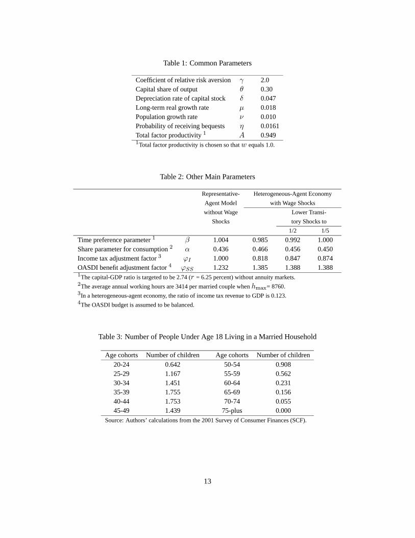
Table 1: Common Parameters

Coefficient of relative risk aversion γ 2.0Capital share of output θ 0.30Depreciation rate of capital stock δ 0.047Long-term real growth rate µ 0.018Population growth rate ν 0.010Probability of receiving bequests η 0.0161Total factor productivity 1 A 0.9491Total factor productivity is chosen so thatw equals 1.0.

Table 2: Other Main Parameters

Representative- Heterogeneous-Agent Economy

Agent Model with Wage Shocks

without Wage Lower Transi-

Shocks tory Shocks to

1/2 1/5

Time preference parameter 1 β 1.004 0.985 0.992 1.000Share parameter for consumption 2 α 0.436 0.466 0.456 0.450Income tax adjustment factor 3 ϕI 1.000 0.818 0.847 0.874OASDI benefit adjustment factor 4 ϕSS 1.232 1.385 1.388 1.3881The capital-GDP ratio is targeted to be 2.74 (r = 6.25 percent) without annuity markets.2The average annual working hours are 3414 per married couple when hmax= 8760.3In a heterogeneous-agent economy, the ratio of income tax revenue to GDP is 0.123.4The OASDI budget is assumed to be balanced.

Table 3: Number of People Under Age 18 Living in a Married Household

Age cohorts Number of children Age cohorts Number of children20-24 0.642 50-54 0.90825-29 1.167 55-59 0.56230-34 1.451 60-64 0.23135-39 1.755 65-69 0.15640-44 1.753 70-74 0.05545-49 1.439 75-plus 0.000

Source: Authors’ calculations from the 2001 Survey of Consumer Finances (SCF).

13

3.1 Households

Utility Function Parameters. The coefficient of relative risk aversion, γ, is assumed to

be 2.0. The number of dependent children at the parents’ age i, ni, is calculated using the

2001 Survey of Consumer Finances (SCF) as shown in Table 3. The “adult equivalency

scale,” ζ, is set at 0.6.10 As discussed later, β is chosen to hit a target capital-output ratio,

producing an interest rate of 6.2 percent in the initial steady state. The maximum working

hours of husband and wife, hmaxi , is set at 8,760, equal to 12 hours per day per person ×365 days× two persons.11 A smaller value for hmaxi would reduce the effective labor supply

elasticity, and tend to reduce the gains from privatization. The parameter α is chosen so that

the average working hours of households between ages 20 and 64 equals 3,414 hours in the

initial steady-state economy, the average number of hours supplied by married households in

the 2001 SCF.

Working Ability. The working ability in this calibration corresponds to the hourly wage

(labor income per hour) of each household in the 2001 SCF.12 The average hourly wage of a

married couple (family members #1 and #2 in SCF) used in the calibration is calculated by

Hourly Wage =Regular and Additional Salaries (#1+ #2) + Payroll Taxes / 2

maxWorking Hours (#1+ #2), 2080.

We adjusted the salaries in the numerator by adding imputed payroll taxes paid by their

employers, which allows us to levy the entire payroll tax on employees in order to incorporate

the payroll tax ceiling. The max operator in the denominator adjusts the hourly wage for a

small fraction of households in the SCF with large reported salaries but few reported working

hours such as the self-employed.

Table 4 shows the eight discrete levels of working abilities of five-year age cohorts. We

use a shape-preserving cubic spline interpolation between each five-year age cohort to obtain10Hence, a married couple with two dependent children must consume about 52 percent (i.e., 20.6 = 1.517)

more than a married couple with no children to attain the same level of utility, ceteris paribus.11The 95th and 99th percentiles of the working hours per married couple of aged 20-64 in the 2001 SCF are

5,280 and 6,375, respectively.12According to Bureau of Labor Statistics data, the average hourly earnings of production workers have in-

creased by 3.8 percent from 2000 to 2001. Since the 2001 SCF wages correspond to year 2000 while our taxfunction introduced below is calibrated to the year 2001, we multiply the SCF wages shown in Table 4 by 1.038to convert the hourly wages in 2000 into growth-adjusted wages in 2001.

14

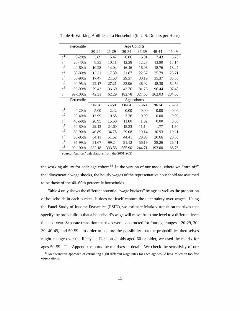
Table 4: Working Abilities of a Household (in U.S. Dollars per Hour)

Percentile Age Cohorts20-24 25-29 30-34 35-39 40-44 45-49

e1 0-20th 3.89 5.47 6.86 6.01 7.43 5.73e2 20-40th 8.35 10.11 12.38 12.27 13.90 13.14e3 40-60th 10.28 14.04 16.46 16.96 18.76 18.47e4 60-80th 12.31 17.30 21.87 22.57 25.79 25.71e5 80-90th 17.47 21.58 29.37 30.19 35.37 35.56e6 90-95th 22.17 27.21 33.96 46.92 48.30 54.59e7 95-99th 29.43 36.60 43.76 81.75 96.44 97.48e8 99-100th 42.31 62.29 182.78 327.65 262.03 284.00

Percentile Age cohorts50-54 55-59 60-64 65-69 70-74 75-79

e1 0-20th 5.00 2.42 0.00 0.00 0.00 0.00e2 20-40th 13.99 10.65 3.36 0.00 0.00 0.00e3 40-60th 20.95 15.60 11.00 1.92 0.00 0.00e4 60-80th 29.13 24.60 18.33 11.14 1.77 1.30e5 80-90th 40.89 34.75 29.08 19.14 10.93 10.21e6 90-95th 54.11 51.62 44.41 29.99 20.66 20.88e7 95-99th 91.67 99.24 91.12 56.19 38.26 26.41e8 99-100th 282.18 333.58 555.90 244.71 193.00 86.76Source: Authors’ calculations from the 2001 SCF.

the working ability for each age cohort.13 In the version of our model where we “turn off”

the idiosyncratic wage shocks, the hourly wages of the representative household are assumed

to be those of the 40–60th percentile households.

Table 4 only shows the different potential “wage buckets” by age as well as the proportion

of households in each bucket. It does not itself capture the uncertainty over wages. Using

the Panel Study of Income Dynamics (PSID), we estimate Markov transition matrixes that

specify the probabilities that a household’s wage will move from one level to a different level

the next year. Separate transition matrixes were constructed for four age ranges—20-29, 30-

39, 40-49, and 50-59—in order to capture the possibility that the probabilities themselves

might change over the lifecycle. For households aged 60 or older, we used the matrix for

ages 50-59. The Appendix reports the matrixes in detail. We check the sensitivity of our13An alternative approach of estimating eight different wage rates for each age would have relied on too few

observations.

15

simulation results to this specification later in the paper.

Population Growth and Mortality. The population growth rate ν is set to one percent per

year, consistent with Social Security Administration (2001) long-run estimates. The survival

rate φi at the end of age i = 20, ..., 109 are the weighted averages of the male and female

survival rates as calculated by SSA. The survival rates at the end of age 109 are replaced by

zero, thereby capping the maximum length of life. See the Appendix for more details.

3.2 Production

Capital and Private Wealth. CapitalK is the sum of private fixed assets and government

fixed assets. In 2000, private fixed assets were $21,165 billion, government fixed assets were

$5,743 billion, and the public held about $3,410 billion of government debt.14 Government

net wealth is set equal to 9.5 percent of total private wealth in the initial steady-state economy.

The time preference parameter β is chosen in each variant of our model explored below so

that the capital-GDP ratio in the initial steady state economy is 2.74, the empirical value in

2000.15

Production Technology. Production takes the Cobb-Douglas form,

F (Kt, Lt) = AtKθt L

1−θt ,

where, recall, Lt is the sum of working hours in efficiency units. The capital share of output

is given by

θ = 1− Compensation of Employees + (1− θ)× Proprietors’ IncomeNational Income + Consumption of Fixed Capital

.

The value of θ in 2000 was 0.30.16 The annual per-capita growth rate µ is assumed to be 1.8

percent, the average rate between 1869 to 1996 (Barro, 1997). Total factor productivity A is

set at 0.949, which normalizes the wage (per efficient labor unit) to unity.14Source: Department of Commerce, Bureau of Economic Analysis.15Ibid.16Source: Department of Commerce, Bureau of Economic Analysis. The average of θ in years between 1996

and 2000 is 0.31.

16

The Depreciation Rate of Fixed Capital. The depreciation rate of fixed capital δ is chosen

by the following steady-state condition,

δ =Total Gross Investment

Fixed Capital− µ− ν.

In 2000, private gross fixed investment accounted for 17.2 percent of GDP, and government

(federal and state) gross investment accounted for 3.3 percent of GDP.17 With a capital-

output ratio of 2.74, the ratio of gross investment to fixed capital is 7.5 percent. Subtracting

productivity and population growth rates, the annual depreciation rate is 4.7 percent.

3.3 The Government

Income Taxes. Federal income tax and state and local taxes are assumed to be at the level

in year 2001 before the passage of the “Economic Growth and Tax Relief Reconciliation Act

of 2001” (EGTRRA). Since households in our model are assumed to be married, we use a

standard deduction of $7,600. Following Altig et al. (2001), we allow higher income house-

holds to itemize deductions when it is more valuable to do so, and we assume that the value

of the itemized deduction increases linearly in the Adjusted Gross Income.18 The additional

exemption per dependent person is $2,900 where the number of dependent children is con-

sistent with Table 3. Table 5 shows the statutory marginal tax rates before EGTRRA.19 As

noted earlier, a household’s labor income in this calibration includes the imputed payroll tax

paid by its employer. Thus, taxable income is obtained by subtracting the employer portion

of payroll tax from labor income.

The standard deduction, the personal exemption, and all tax brackets grow with produc-

tivity over time so that there is no real bracket creep; this indexing is also needed for the

initial economy to be in steady state. Also, since the effective tax rate on capital income

is reduced by investment tax incentives, accelerated depreciation and other factors (Auer-

bach, 1996), the tax function is further adjusted so that the cross-sectional average tax rate17Ibid.18In particular, the deduction taken by a household is the greater of the standard deduction and 0.0755×AGI,

ormax$7600, 0.0755×AGI.19The key qualitative results reported herein are unaffected if the tax function were instead modeled as net

taxes, that is, after substracting transfers indicated in the Statistics of Income.

17

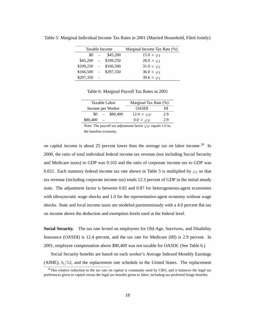
Table 5: Marginal Individual Income Tax Rates in 2001 (Married Household, Filed Jointly)

Taxable Income Marginal Income Tax Rate (%)$0 – $45,200 15.0× ϕI

$45,200 – $109,250 28.0× ϕI$109,250 – $166,500 31.0× ϕI$166,500 – $297,350 36.0× ϕI$297,350 – 39.6× ϕI

Table 6: Marginal Payroll Tax Rates in 2001

Taxable Labor Marginal Tax Rate (%)Income per Worker OASDI HI

$0 – $80,400 12.4× ϕP 2.9$80,400 – 0.0× ϕP 2.9Note: The payroll tax adjustment factor ϕP equals 1.0 in.

the baseline economy.

on capital income is about 25 percent lower than the average tax on labor income.20 In

2000, the ratio of total individual federal income tax revenue (not including Social Security

and Medicare taxes) to GDP was 0.102 and the ratio of corporate income tax to GDP was

0.021. Each statutory federal income tax rate shown in Table 5 is multiplied by ϕI so that

tax revenue (including corporate income tax) totals 12.3 percent of GDP in the initial steady

state. The adjustment factor is between 0.82 and 0.87 for heterogeneous-agent economies

with idiosyncratic wage shocks and 1.0 for the representative-agent economy without wage

shocks. State and local income taxes are modeled parsimoniously with a 4.0 percent flat tax

on income above the deduction and exemption levels used at the federal level.

Social Security. The tax rate levied on employees for Old-Age, Survivors, and Disability

Insurance (OASDI) is 12.4 percent, and the tax rate for Medicare (HI) is 2.9 percent. In

2001, employee compensation above $80,400 was not taxable for OASDI. (See Table 6.)

Social Security benefits are based on each worker’s Average Indexed Monthly Earnings

(AIME), bi/12, and the replacement rate schedule in the United States. The replacement20This relative reduction to the tax rate on capital is commonly used by CBO, and it balances the legal tax

preferences given to capital versus the legal tax benefits given to labor, including tax-preferred fringe benefits.

18

Table 7: OASDI Replacement Rates in 2001

AIME (b/12) Marginal Replacement Rate (%)$0 – $561 90.0× ϕSS

$561 – $3,381 32.0× ϕSS$3,381 – 15.0× ϕSSNote: The OASDI benefit adjustment factor ϕSS is set so

that the OASDI is pay-as-you-go in the baseline economies.

rates are 90 percent for the first $561, 32 percent for amounts between $561 and $3,381,

and 15 percent for amounts above $3,381. Social Security, therefore, is progressive in that a

worker’s benefit relative to AIME (the “replacement rate”) is decreasing in the AIME.

The U.S. OASDI also pays spousal, survivors’ and disability benefits in addition to the

standard retirement benefit described above. Indeed, retiree benefits accounted for only 69.1

percent of total OASDI benefits in December 2000.21 OASDI benefits are adjusted upward

by the proportional adjustment factor ϕSS so that total benefit payments equal total payroll

tax revenue. The adjustment factor ϕSS equals about 1.39 in our model with wage shocks

and 1.23 in our model without wage shocks. This adjustment proportionally distributes non-

retiree OASDI payments across retirees.

4 Policy Experiments

We simulate a stylized phased-in partial privatization of Social Security that begins in

year 1. Workers immediately start redirecting 50 percent of their payroll tax payments into

private saving accounts. As is implicit in most previous work on privatization, assets in the

new private accounts are assumed to be perfect substitutes with other private assets, including

earning the same market rate of return and being subject to the same income tax schedule, as

outlined above. As a result, the new private accounts do not have to be explicitly modeled;

the redirected payroll simply increases regular household saving.

Social Security benefits are reduced linearly over time. Households age 66 and older

in year 1 receive the current-law (baseline) benefits throughout the rest of their lifetime;

households of age 65 in year 1 receive benefits that are 1.25 percent lower than the current-21See Table 5.A1 in Social Security Administration (2001).

19

law level throughout the rest of lifetime; households of age 64 in year 1 receive benefits 2.5

percent lower than the current law-level, and so on. Households age 25 or younger in year 1

receive one half of their traditional Social Security benefits when they turn 65.

Since benefit payments are reduced more slowly than payroll taxes during the transitional

period, Social Security faces a cash-flow deficit that we finance with a consumption tax;work

by Kotlikoff, Smetters and Walliser (2001) also focused on consumption tax financing as a

method of producing the largest macroeconomic gains from privatization. Since changes

to the Social Security system will also influence the size of the capital stock and, hence,

non-Social Security government receipts, the rest of the government budget is balanced by

proportional changes in marginal income tax rates.

We first consider the representative-agent economy without wage shocks (equivalently,

with insurable wage shocks) where all households have the wage profile of the 40–60th

percentile in Table 4, i.e., lifetime income group e3. We then turn to a heterogeneous-agent

economy with uninsurable wage shocks. We initially assume that both economies are closed

to international capital flows and that a private annuity market does not exist.

4.1 Representative-Agent Economy without Wage Shocks

As shown in Run 1 in Table 8, partial privatization of Social Security in the representative-

agent economy increases national wealth by 20.7 percent in the long run compared to the

baseline economy. GNP increases by 9.3 percent in the long run, while labor supply in-

creases by 4.8 percent. These large gains are driven by pre-funding a portion of Social

Security’s liabilities that were previously financed on a pay-as-you-go (unfunded) basis.

Moreover, national wealth and GNP increase throughout the entire transition path. La-

bor supply initially increases by 3.4 percent in the first year as households reoptimize their

lifecycle choices after the policy change. Then, it declines slightly between years 1 and 20

after the reform before eventually increasing. The reason for this non-monotonic behavior

is two-fold. First, as shown in Table 8, labor supply increases faster than capital during part

of the first decade after reform, briefly decreasing the wage rate by about 1 percent. Sec-

ond, the new temporary consumption tax, which starts at 6.5 percent and comes down over

time as Social Security benefits are gradually reduced, discourages labor supply during the

20

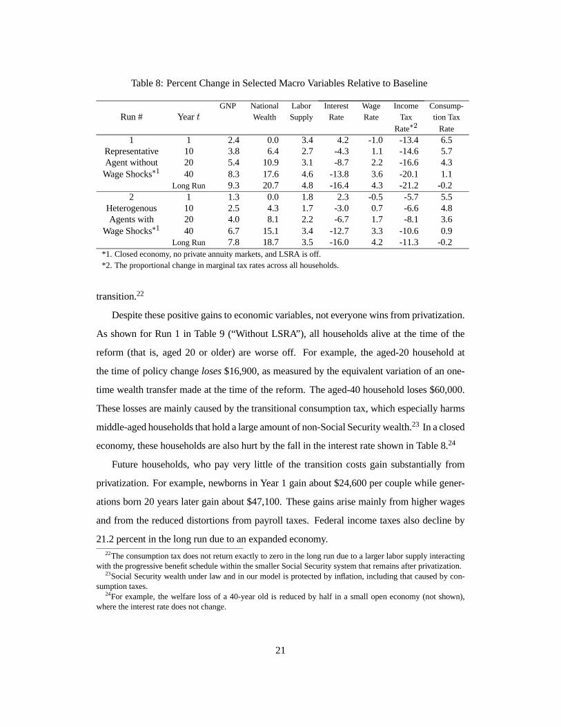
Table 8: Percent Change in Selected Macro Variables Relative to Baseline

GNP National Labor Interest Wage Income Consump-Run # Year t Wealth Supply Rate Rate Tax tion Tax

Rate∗2 Rate

1 1 2.4 0.0 3.4 4.2 -1.0 -13.4 6.5Representative 10 3.8 6.4 2.7 -4.3 1.1 -14.6 5.7Agent without 20 5.4 10.9 3.1 -8.7 2.2 -16.6 4.3Wage Shocks∗1 40 8.3 17.6 4.6 -13.8 3.6 -20.1 1.1

Long Run 9.3 20.7 4.8 -16.4 4.3 -21.2 -0.22 1 1.3 0.0 1.8 2.3 -0.5 -5.7 5.5

Heterogenous 10 2.5 4.3 1.7 -3.0 0.7 -6.6 4.8Agents with 20 4.0 8.1 2.2 -6.7 1.7 -8.1 3.6

Wage Shocks∗1 40 6.7 15.1 3.4 -12.7 3.3 -10.6 0.9Long Run 7.8 18.7 3.5 -16.0 4.2 -11.3 -0.2

*1. Closed economy, no private annuity markets, and LSRA is off.*2. The proportional change in marginal tax rates across all households.

transition.22

Despite these positive gains to economic variables, not everyone wins from privatization.

As shown for Run 1 in Table 9 (“Without LSRA”), all households alive at the time of the

reform (that is, aged 20 or older) are worse off. For example, the aged-20 household at

the time of policy change loses $16,900, as measured by the equivalent variation of an one-

time wealth transfer made at the time of the reform. The aged-40 household loses $60,000.

These losses are mainly caused by the transitional consumption tax, which especially harms

middle-aged households that hold a large amount of non-Social Security wealth.23 In a closed

economy, these households are also hurt by the fall in the interest rate shown in Table 8.24

Future households, who pay very little of the transition costs gain substantially from

privatization. For example, newborns in Year 1 gain about $24,600 per couple while gener-

ations born 20 years later gain about $47,100. These gains arise mainly from higher wages

and from the reduced distortions from payroll taxes. Federal income taxes also decline by

21.2 percent in the long run due to an expanded economy.22The consumption tax does not return exactly to zero in the long run due to a larger labor supply interacting

with the progressive benefit schedule within the smaller Social Security system that remains after privatization.23Social Security wealth under law and in our model is protected by inflation, including that caused by con-

sumption taxes.24For example, the welfare loss of a 40-year old is reduced by half in a small open economy (not shown),

where the interest rate does not change.

21

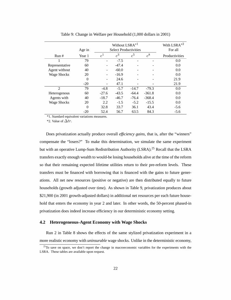
Table 9: Change in Welfare per Household (1,000 dollars in 2001)

Without LSRA∗1 With LSRA∗2Age in Select Productivities For all

Run # Year 1 e1 e3 e5 e8 Productivities1 79 - -7.5 - - 0.0

Representative 60 - -47.4 - - 0.0Agent without 40 - -60.0 - - 0.0Wage Shocks 20 - -16.9 - - 0.0

0 - 24.6 - - 21.9-20 - 47.1 - - 21.9

2 79 -4.8 -5.7 -14.7 -79.3 0.0Heterogenous 60 -27.6 -43.5 -64.4 -361.8 0.0Agents with 40 -18.7 -46.7 -76.4 -368.4 0.0Wage Shocks 20 2.2 -1.5 -5.2 -15.5 0.0

0 32.8 33.7 36.1 43.4 -5.6-20 52.4 56.7 63.5 84.3 -5.6

*1. Standard equivalent variations measures.*2. Value of∆tr.

Does privatization actually produce overall efficiency gains, that is, after the “winners”

compensate the “losers?” To make this determination, we simulate the same experiment

but with an operative Lump-Sum Redistribution Authority (LSRA).25 Recall that the LSRA

transfers exactly enough wealth to would-be losing households alive at the time of the reform

so that their remaining expected lifetime utilities return to their pre-reform levels. These

transfers must be financed with borrowing that is financed with the gains to future gener-

ations. All net new resources (positive or negative) are then distributed equally to future

households (growth adjusted over time). As shown in Table 9, privatization produces about

$21,900 (in 2001 growth-adjusted dollars) in additional net resources per each future house-

hold that enters the economy in year 2 and later. In other words, the 50-percent phased-in

privatization does indeed increase efficiency in our deterministic economy setting.

4.2 Heterogeneous-Agent Economy with Wage Shocks

Run 2 in Table 8 shows the effects of the same stylized privatization experiment in a

more realistic economy with uninsurable wage shocks. Unlike in the deterministic economy,25To save on space, we don’t report the change in macroeconomic variables for the experiments with the

LSRA. These tables are available upon request.

22

Social Security’s progressive benefit formula now provides some risk sharing that is unattain-

able in the private market. National wealth now increases by 18.7 percent in the long run, but

by less than in the representative-agent economy (Run 1) because a portion of private saving

is now for precautionary motives, which is less sensitive to changes in Social Security policy.

Labor supply increases by 3.5 percent in the long run and GNP is 7.8 percent higher.

Similar to the representative-agent economy, most households alive at the time of the

reform are worse off because they have to pay higher taxes to finance the transition. Run

2 in Table 9 shows that relatively high wage (and, hence, wealthier) households tend to be

hit the hardest by the consumption tax. For example, a 40-year old in the top one percent

of the wage distribution (e8) at the time of privatization loses $368,400. As with Run 1,

future households gain considerably from the lower payroll and income tax rates as well as

higher wages. Even households in the lowest 20 percent of the wage distribution (e1) born 20

years later gain $52,400 (in 2001 growth-adjusted dollars). Overall, privatization, though, no

longer improves efficiency. After the LSRA returns the welfare of all households to their pre-

reform levels, it distributes a negative $5,600 to each future household. This loss contrasts

sharply with the gain of $21,900 in the deterministic economy discussed above.

4.3 Alternative Experiments in the Heterogeneous-Agent Economy

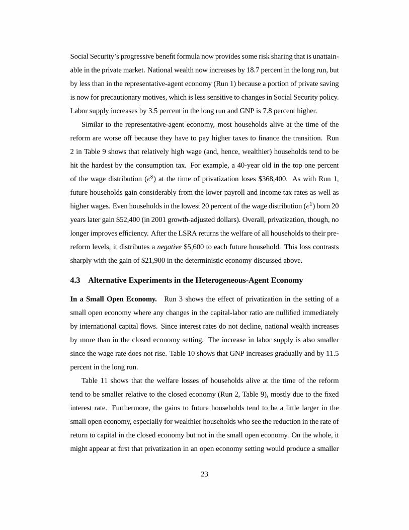
In a Small Open Economy. Run 3 shows the effect of privatization in the setting of a

small open economy where any changes in the capital-labor ratio are nullified immediately

by international capital flows. Since interest rates do not decline, national wealth increases

by more than in the closed economy setting. The increase in labor supply is also smaller

since the wage rate does not rise. Table 10 shows that GNP increases gradually and by 11.5

percent in the long run.

Table 11 shows that the welfare losses of households alive at the time of the reform

tend to be smaller relative to the closed economy (Run 2, Table 9), mostly due to the fixed

interest rate. Furthermore, the gains to future households tend to be a little larger in the

small open economy, especially for wealthier households who see the reduction in the rate of

return to capital in the closed economy but not in the small open economy. On the whole, it

might appear at first that privatization in an open economy setting would produce a smaller

23

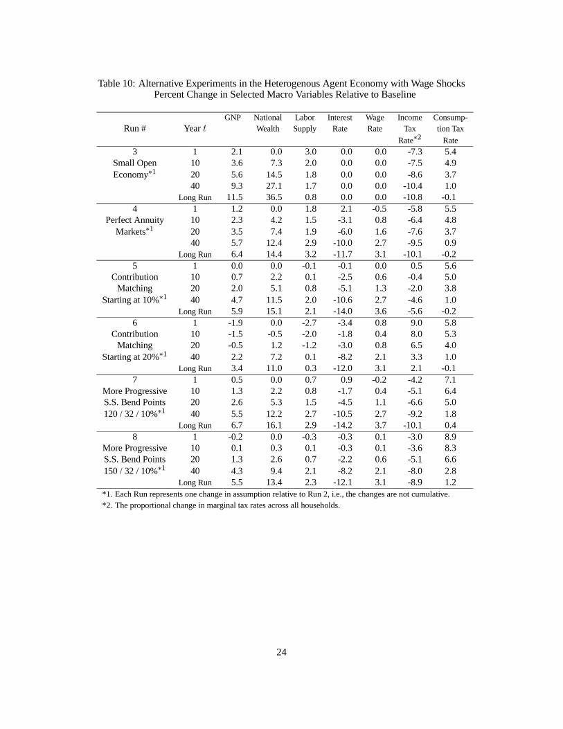
Table 10: Alternative Experiments in the Heterogenous Agent Economy with Wage ShocksPercent Change in Selected Macro Variables Relative to Baseline

GNP National Labor Interest Wage Income Consump-Run # Year t Wealth Supply Rate Rate Tax tion Tax

Rate∗2 Rate3 1 2.1 0.0 3.0 0.0 0.0 -7.3 5.4

Small Open 10 3.6 7.3 2.0 0.0 0.0 -7.5 4.9Economy∗1 20 5.6 14.5 1.8 0.0 0.0 -8.6 3.7

40 9.3 27.1 1.7 0.0 0.0 -10.4 1.0Long Run 11.5 36.5 0.8 0.0 0.0 -10.8 -0.1

4 1 1.2 0.0 1.8 2.1 -0.5 -5.8 5.5Perfect Annuity 10 2.3 4.2 1.5 -3.1 0.8 -6.4 4.8

Markets∗1 20 3.5 7.4 1.9 -6.0 1.6 -7.6 3.740 5.7 12.4 2.9 -10.0 2.7 -9.5 0.9

Long Run 6.4 14.4 3.2 -11.7 3.1 -10.1 -0.25 1 0.0 0.0 -0.1 -0.1 0.0 0.5 5.6

Contribution 10 0.7 2.2 0.1 -2.5 0.6 -0.4 5.0Matching 20 2.0 5.1 0.8 -5.1 1.3 -2.0 3.8

Starting at 10%∗1 40 4.7 11.5 2.0 -10.6 2.7 -4.6 1.0Long Run 5.9 15.1 2.1 -14.0 3.6 -5.6 -0.2

6 1 -1.9 0.0 -2.7 -3.4 0.8 9.0 5.8Contribution 10 -1.5 -0.5 -2.0 -1.8 0.4 8.0 5.3

Matching 20 -0.5 1.2 -1.2 -3.0 0.8 6.5 4.0Starting at 20%∗1 40 2.2 7.2 0.1 -8.2 2.1 3.3 1.0

Long Run 3.4 11.0 0.3 -12.0 3.1 2.1 -0.17 1 0.5 0.0 0.7 0.9 -0.2 -4.2 7.1

More Progressive 10 1.3 2.2 0.8 -1.7 0.4 -5.1 6.4S.S. Bend Points 20 2.6 5.3 1.5 -4.5 1.1 -6.6 5.0120 / 32 / 10%∗1 40 5.5 12.2 2.7 -10.5 2.7 -9.2 1.8

Long Run 6.7 16.1 2.9 -14.2 3.7 -10.1 0.48 1 -0.2 0.0 -0.3 -0.3 0.1 -3.0 8.9

More Progressive 10 0.1 0.3 0.1 -0.3 0.1 -3.6 8.3S.S. Bend Points 20 1.3 2.6 0.7 -2.2 0.6 -5.1 6.6150 / 32 / 10%∗1 40 4.3 9.4 2.1 -8.2 2.1 -8.0 2.8

Long Run 5.5 13.4 2.3 -12.1 3.1 -8.9 1.2*1. Each Run represents one change in assumption relative to Run 2, i.e., the changes are not cumulative.*2. The proportional change in marginal tax rates across all households.

24

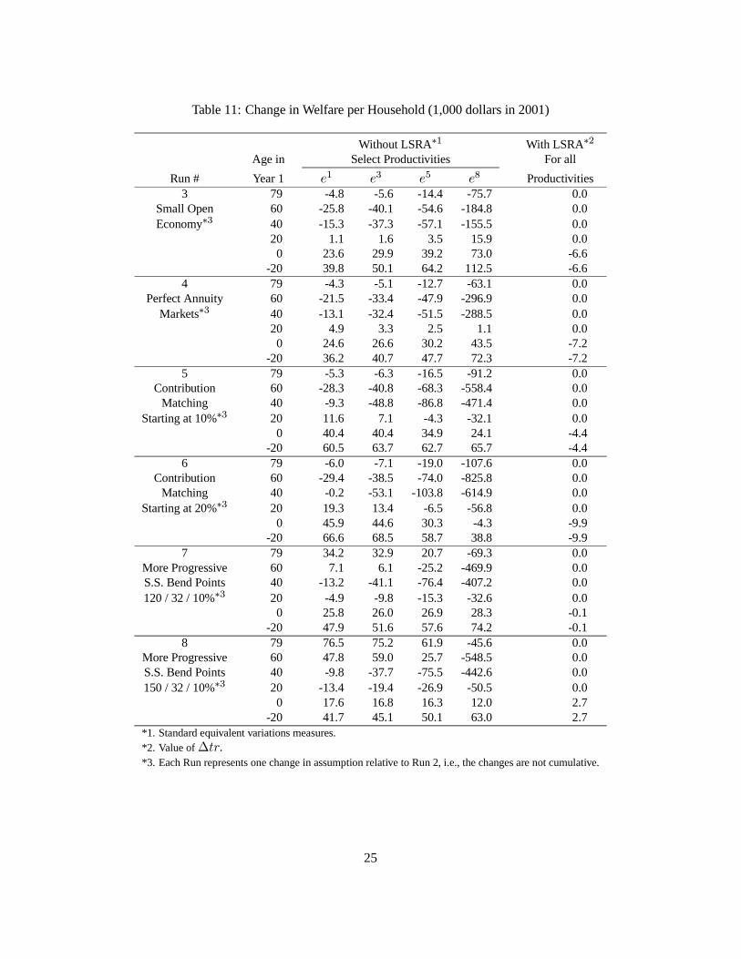
Table 11: Change in Welfare per Household (1,000 dollars in 2001)

Without LSRA∗1 With LSRA∗2Age in Select Productivities For all

Run # Year 1 e1 e3 e5 e8 Productivities3 79 -4.8 -5.6 -14.4 -75.7 0.0

Small Open 60 -25.8 -40.1 -54.6 -184.8 0.0Economy∗3 40 -15.3 -37.3 -57.1 -155.5 0.0

20 1.1 1.6 3.5 15.9 0.00 23.6 29.9 39.2 73.0 -6.6

-20 39.8 50.1 64.2 112.5 -6.64 79 -4.3 -5.1 -12.7 -63.1 0.0

Perfect Annuity 60 -21.5 -33.4 -47.9 -296.9 0.0Markets∗3 40 -13.1 -32.4 -51.5 -288.5 0.0

20 4.9 3.3 2.5 1.1 0.00 24.6 26.6 30.2 43.5 -7.2

-20 36.2 40.7 47.7 72.3 -7.25 79 -5.3 -6.3 -16.5 -91.2 0.0

Contribution 60 -28.3 -40.8 -68.3 -558.4 0.0Matching 40 -9.3 -48.8 -86.8 -471.4 0.0

Starting at 10%∗3 20 11.6 7.1 -4.3 -32.1 0.00 40.4 40.4 34.9 24.1 -4.4

-20 60.5 63.7 62.7 65.7 -4.46 79 -6.0 -7.1 -19.0 -107.6 0.0

Contribution 60 -29.4 -38.5 -74.0 -825.8 0.0Matching 40 -0.2 -53.1 -103.8 -614.9 0.0

Starting at 20%∗3 20 19.3 13.4 -6.5 -56.8 0.00 45.9 44.6 30.3 -4.3 -9.9

-20 66.6 68.5 58.7 38.8 -9.97 79 34.2 32.9 20.7 -69.3 0.0

More Progressive 60 7.1 6.1 -25.2 -469.9 0.0S.S. Bend Points 40 -13.2 -41.1 -76.4 -407.2 0.0120 / 32 / 10%∗3 20 -4.9 -9.8 -15.3 -32.6 0.0

0 25.8 26.0 26.9 28.3 -0.1-20 47.9 51.6 57.6 74.2 -0.1

8 79 76.5 75.2 61.9 -45.6 0.0More Progressive 60 47.8 59.0 25.7 -548.5 0.0S.S. Bend Points 40 -9.8 -37.7 -75.5 -442.6 0.0150 / 32 / 10%∗3 20 -13.4 -19.4 -26.9 -50.5 0.0

0 17.6 16.8 16.3 12.0 2.7-20 41.7 45.1 50.1 63.0 2.7

*1. Standard equivalent variations measures.*2. Value of∆tr.*3. Each Run represents one change in assumption relative to Run 2, i.e., the changes are not cumulative.

25

efficiency loss than in the closed economy. This hunch is incorrect. When the LSRA is

operative, Table 11 shows that the efficiency losses are actually slightly larger in the small

open economy, equal to $6,600 per each future household. The reason is that the LSRA’s

cost of borrowing is higher in the small open economy setting since the interest rate does not

decrease over time.

Perfect Annuity Markets. Thus far, we have assumed private annuity markets do not exist

and so, in addition to sharing wage uncertainty, the Social Security system shares longevity

uncertainty in a way the private market cannot. It would appear at first glance that privati-

zation has a better chance of producing efficiency gains if we instead assumed that a private

annuity market is available. This intuition also turns out to be incorrect.

Run 4 in Table 11 shows that the efficiency losses are actually larger with perfect private

annuity markets than without (Run 2). In particular, each household loses $7,200, compared

to $5,600 shown earlier (Run 2, Table 9) without an annuity market. As shown for Run 2

in Table 8, privatization without a private annuity market leads to a 18.7 percent increase

in national wealth in the long run, which is larger than the 14.4 percent increase for Run 4

shown in Table 10. The reason is that households increase their precautionary savings in Run

2 as the annuity insurance provided by Social Security is reduced; in contrast, households

can rely more on the private annuity market rather than precautionary savings in Run 4. The

smaller amount of precautionary savings in Run 4 produces larger efficiency losses for three

reasons: (i) the LSRA must borrow at a higher interest rate; (ii) income taxes are higher

since there is less capital and labor income; and (iii) the interest elasticity of saving is higher,

increasing the role that falling interest rates have on discouraging additional saving.

Contribution Matching. The pre-reform Social Security system is progressive by giving

households with a lower average index of pre-retirement wages a larger Social Security ben-

efit relative to their pre-retirement wages, that is, a higher “replacement rate.” To be sure,

the privatized experiment considered above preserves some progressivity by reducing bene-

fits proportionally only by half in the long run—the poor still get a larger replacement rate.

Yet, a proportional reduction in benefits still reduces progressivity; for example, reducing all

26

benefits by 100 percent would eliminate progressivity.

Run 5 considers privatization with a progressive contribution match. In particular, work-

ing households with low levels of labor income receive a fairly generous match equal to

10 percent of their earnings. This matching rate declines linearly to zero as labor income

approaches $60,000, which is slightly above the median household income in the model

economy.26 While ensuing Social Security deficits continue to be financed with a consump-

tion tax, the contribution match is financed each year by increasing the marginal income tax

rates proportionally across all households; the key qualitative results would be unchanged if

the consumption tax were used instead. As before, income tax rates are changed so that the

rest of government budget is balanced throughout the transition path.

As shown in Run 5 in Table 10, privatization with contribution matching increases na-

tional wealth, GNP and labor supply throughout the transition path compared to the pre-

reform baseline economy. However, the long-run increases in national wealth, labor supply,

and GNP are smaller relative to the case without contribution matching (Run 2 in Table 8)

since the match must be financed with a distorting income tax. In the long run, GNP increases

by only 5.9 percent, compared to 7.8 percent without the match.

The welfare gains for Run 5 reported in Table 11 show that contribution matching tends

to improve the welfare of poorer households relative to Run 2 without the match. Whereas

the poorest household born in the future gains $52,400 without the match, they gain $60,500

with the match. Not surprisingly, the richest households are worse off since they don’t receive

any of the match but must help finance it; they gained $84,300 without the match in the long

run but only $65,700 with the match. With the LSRA, privatization still leads to efficiency

losses, equal to about $4,400 (in 2001 growth-adjusted dollars) per future household. Yet,

this loss is smaller than the $5,600 loss without the match.

Run 6 doubles the starting match rate from 10 percent at zero wage income to 20 percent.

As before, this match declines linearly to zero as labor income approaches $60,000. Table

11 shows that, with the LSRA, this more generous match produced efficiency losses equal to

$9,900 per future household, which is larger in magnitude relative to the 10 percent match26This matching schedule is equivalent with the marginal labor income tax of -10 percent at $0 of labor income,

0 percent at $30,000, 10 percent at $60,000, and 0 percent for labor income above $60,000.

27

and even Run 2 without any match. This non-monotonic behavior is due to the trade-off

between risk sharing and labor supply distortions: some match is beneficial but is dominated

by distortions at higher tax rates.27 In fact, there is no match rate that allows privatization

to produced efficiency gains. Moreover, several alternative designs of contribution matching

performed even worse.28

Progressive Benefit Schedule. Run 7 takes a different approach to maintaining some pro-

gressivity after privatization. It immediately increases the progressivity of the Social Secu-

rity benefit that remains after privatization by raising the replacement rate of the lowest wage

income bracket from 90 percent to 120 percent while reducing the replacement rate of the

highest wage income bracket from 15 percent to 10 percent. Run 8 is even more aggressive in

redistribution by raising the replacement rate of the lowest wage income bracket to 150 per-

cent. Table 11 shows that this approach is especially effective at protecting the welfare of the

poor at the time of reform as well as reducing efficiency losses. Now, privatization reduces

efficiency by only $100 per future household under the LSRA in Run 8. However, privati-

zation actually increases efficiency by $2,700 per future household in Run 8. Increasing the

progressivity of the smaller Social Security system that remains after privatization is more

efficient than contribution matching because a considerable amount of redistribution can be

accomplished with less distortion to labor supply, that is, with smaller effective tax rates at

the margin. In particular, whereas contribution matching is based on the labor income in any

given year, Social Security’s progressive benefit is based on a household’s lifetime earnings,

which is harder to change.27These distortions arise from both the income tax used to finance the match as well as the effective marginal

tax rates caused by the match itself.28For example, a proportional match for all households performed worse because, while eliminating implicit

marginal tax rates in the phase-out range, enhanced the income tax distortions since more revenue is needed.We also considered financing the phased-out match with a negative match on those with above-average incomes.Although potentially more efficient at redistribution than an income tax, as the poor are not financing their ownmatch, it also performed worse. Labor supply tends to be fairly elastic in our model whereas the savings elasticityis relatively low with precautionary saving.

28

Table 12: Alternative Transitory ShocksPercent Change in Selected Macro Variables Relative to Baseline

GNP National Labor Interest Wage Income Consump-Run # Year t Wealth Supply Rate Rate Tax tion Tax

Rate∗2 Rate

9 1 1.5 0.0 2.2 2.7 -0.7 -6.3 5.612 Transitory 10 3.0 5.0 2.1 -3.4 0.8 -7.5 4.9Shocks∗1 20 4.6 9.4 2.6 -7.7 1.9 -9.2 3.7

40 7.5 16.6 3.8 -13.7 3.6 -11.7 0.9Long Run 8.7 20.4 4.0 -17.1 4.5 -12.6 -0.3

10 1 1.6 0.0 2.3 2.8 -0.7 -6.4 5.715 Transitory 10 3.1 5.4 2.2 -3.8 0.9 -7.8 5.0Shocks∗1 20 4.9 10.1 2.7 -8.3 2.1 -9.6 3.7

40 7.9 17.4 4.0 -14.3 3.7 -12.4 0.9Long Run 9.1 21.4 4.2 -17.8 4.7 -13.4 -0.3

*1. Each Run represents one change in assumption relative to Run 2, i.e., the changes are not cumulative.*2. The proportional change in marginal tax rates across all households.

4.4 Alternative Assumptions of Transitory Shocks and Persistence

A key assumption in our model is the size of the transitory working ability shocks and

their persistence. Recall that we constructed the age-working ability schedule from the 2001

Survey of Consumer Finances (SCF) and the transition matrices from the 1989-92 Panel

Study of Income Dynamics (PSID). To deal with possible measurement errors, our bench-

mark Markov transition matrixes are calculated after taking three-year moving averages of

workers’ hourly wages. This ad hoc treatment reduces the size of transitory wage shocks in

the original data by about one-third. Floden and Lindé (2001) argue that measurement error

in the PSID might be as large as the size of the real fluctuation. Thus, although we have

already “smoothed away” some of that error by focusing on three-year moving averages, the

transitory shocks in our model might still be too large.

Run 9 shown in Tables 12 and 13 show the economic and welfare effects, respectively,

of privatization when the transitory shocks are reduced to only half of their previous values

we used in the main calibration. Run 10 goes even further: it reduces the shocks to only

one-fifth of the values under the main calibration. National wealth increases by 20.4 percent

in the long run in Run 9, compared to 18.7 percent for Run 2. However, the efficiency losses

actually increase to $8,200 per future household (relative to a $5,600 loss in Run 2) under the

29

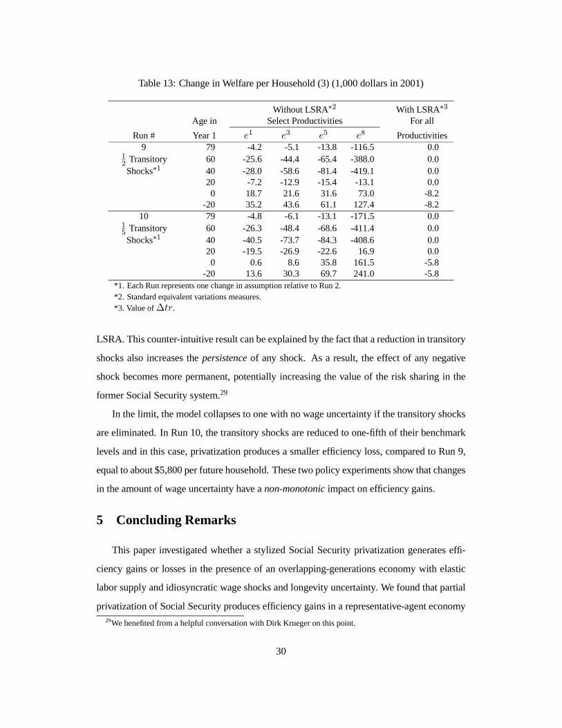
Table 13: Change in Welfare per Household (3) (1,000 dollars in 2001)

Without LSRA∗2 With LSRA∗3Age in Select Productivities For all

Run # Year 1 e1 e3 e5 e8 Productivities9 79 -4.2 -5.1 -13.8 -116.5 0.0

12 Transitory 60 -25.6 -44.4 -65.4 -388.0 0.0Shocks∗1 40 -28.0 -58.6 -81.4 -419.1 0.0

20 -7.2 -12.9 -15.4 -13.1 0.00 18.7 21.6 31.6 73.0 -8.2

-20 35.2 43.6 61.1 127.4 -8.210 79 -4.8 -6.1 -13.1 -171.5 0.0

15 Transitory 60 -26.3 -48.4 -68.6 -411.4 0.0Shocks∗1 40 -40.5 -73.7 -84.3 -408.6 0.0

20 -19.5 -26.9 -22.6 16.9 0.00 0.6 8.6 35.8 161.5 -5.8

-20 13.6 30.3 69.7 241.0 -5.8*1. Each Run represents one change in assumption relative to Run 2.*2. Standard equivalent variations measures.*3. Value of∆tr.

LSRA. This counter-intuitive result can be explained by the fact that a reduction in transitory

shocks also increases the persistence of any shock. As a result, the effect of any negative

shock becomes more permanent, potentially increasing the value of the risk sharing in the

former Social Security system.29

In the limit, the model collapses to one with no wage uncertainty if the transitory shocks

are eliminated. In Run 10, the transitory shocks are reduced to one-fifth of their benchmark

levels and in this case, privatization produces a smaller efficiency loss, compared to Run 9,

equal to about $5,800 per future household. These two policy experiments show that changes

in the amount of wage uncertainty have a non-monotonic impact on efficiency gains.

5 Concluding Remarks

This paper investigated whether a stylized Social Security privatization generates effi-

ciency gains or losses in the presence of an overlapping-generations economy with elastic

labor supply and idiosyncratic wage shocks and longevity uncertainty. We found that partial

privatization of Social Security produces efficiency gains in a representative-agent economy29We benefited from a helpful conversation with Dirk Krueger on this point.

30

without wage shocks (or, equivalently, if these shocks are insurable). In a heterogeneous-

agent economy with idiosyncratic and uninsurable wage shocks, however, the overall ef-

ficiency of the economy is reduced by our stylized privatization since the existing Social

Security system provides a valuable source of risk sharing through its progressive benefit

formula. This result was fairly robust to a wide range of model considerations: (i) the degree

of openness of the economy; (ii) allowing the availability of actuarially-fair private annu-

ities; (iii) the introduction of various risk-sharing mechanisms after privatization; and (iv)

reducing by half the size of transitory wage shocks. Only in the case in which the benefit

replacement rate of the lowest bracket was increased to 150 percent from 90 percent did we

find efficiency gains. Rather surprisingly, privatization performs relatively better in a closed

economy where the rate of return falls as capital is accumulated and even when private an-

nuity markets do not exist. Furthermore, matching the contribution of poorer workers can

actually do more harm than good, whereas increasing the progressivity of the Social Security

system that remains works well.

One of the possible limitations of our model is that it does not distinguish by various

demographic groups, including race and gender. There is some evidence, for example, that

black Americans do not live as long as non-blacks, even after controlling for differences in

earnings. Blacks are also less likely to be married at the point of retirement and, therefore,

less likely to qualify for a spousal benefit.30 In contrast, women have a higher life expectancy

than males, and they might also face a higher effective marginal tax rate on their contribu-

tions if they are the household’s secondary earner. Incorporating these additional sources of

heterogeneity would possibly change the welfare implications of this paper.30See, for example, Gustman and Steinmeier (2001).

31

Appendices

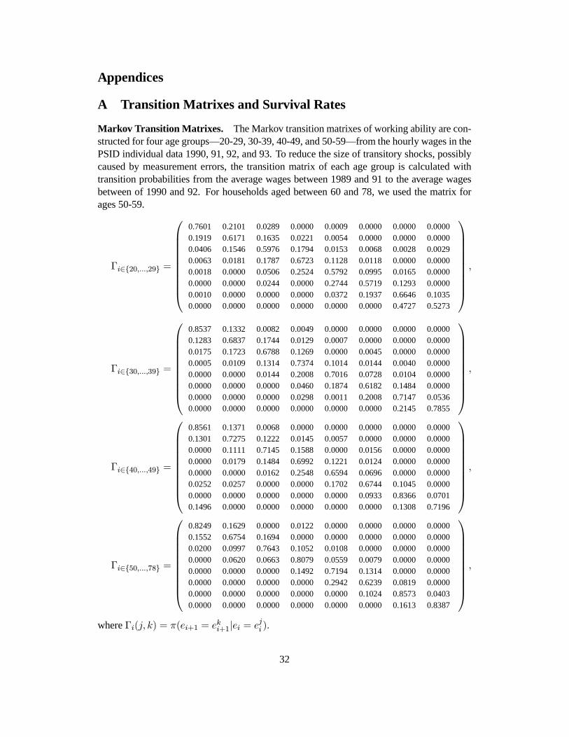
A Transition Matrixes and Survival Rates

Markov Transition Matrixes. The Markov transition matrixes of working ability are con-structed for four age groups—20-29, 30-39, 40-49, and 50-59—from the hourly wages in thePSID individual data 1990, 91, 92, and 93. To reduce the size of transitory shocks, possiblycaused by measurement errors, the transition matrix of each age group is calculated withtransition probabilities from the average wages between 1989 and 91 to the average wagesbetween of 1990 and 92. For households aged between 60 and 78, we used the matrix forages 50-59.

Γi∈20,...,29 =

0.7601 0.2101 0.0289 0.0000 0.0009 0.0000 0.0000 0.00000.1919 0.6171 0.1635 0.0221 0.0054 0.0000 0.0000 0.00000.0406 0.1546 0.5976 0.1794 0.0153 0.0068 0.0028 0.00290.0063 0.0181 0.1787 0.6723 0.1128 0.0118 0.0000 0.00000.0018 0.0000 0.0506 0.2524 0.5792 0.0995 0.0165 0.00000.0000 0.0000 0.0244 0.0000 0.2744 0.5719 0.1293 0.00000.0010 0.0000 0.0000 0.0000 0.0372 0.1937 0.6646 0.10350.0000 0.0000 0.0000 0.0000 0.0000 0.0000 0.4727 0.5273

,

Γi∈30,...,39 =

0.8537 0.1332 0.0082 0.0049 0.0000 0.0000 0.0000 0.00000.1283 0.6837 0.1744 0.0129 0.0007 0.0000 0.0000 0.00000.0175 0.1723 0.6788 0.1269 0.0000 0.0045 0.0000 0.00000.0005 0.0109 0.1314 0.7374 0.1014 0.0144 0.0040 0.00000.0000 0.0000 0.0144 0.2008 0.7016 0.0728 0.0104 0.00000.0000 0.0000 0.0000 0.0460 0.1874 0.6182 0.1484 0.00000.0000 0.0000 0.0000 0.0298 0.0011 0.2008 0.7147 0.05360.0000 0.0000 0.0000 0.0000 0.0000 0.0000 0.2145 0.7855

,

Γi∈40,...,49 =

0.8561 0.1371 0.0068 0.0000 0.0000 0.0000 0.0000 0.00000.1301 0.7275 0.1222 0.0145 0.0057 0.0000 0.0000 0.00000.0000 0.1111 0.7145 0.1588 0.0000 0.0156 0.0000 0.00000.0000 0.0179 0.1484 0.6992 0.1221 0.0124 0.0000 0.00000.0000 0.0000 0.0162 0.2548 0.6594 0.0696 0.0000 0.00000.0252 0.0257 0.0000 0.0000 0.1702 0.6744 0.1045 0.00000.0000 0.0000 0.0000 0.0000 0.0000 0.0933 0.8366 0.07010.1496 0.0000 0.0000 0.0000 0.0000 0.0000 0.1308 0.7196

,

Γi∈50,...,78 =

0.8249 0.1629 0.0000 0.0122 0.0000 0.0000 0.0000 0.00000.1552 0.6754 0.1694 0.0000 0.0000 0.0000 0.0000 0.00000.0200 0.0997 0.7643 0.1052 0.0108 0.0000 0.0000 0.00000.0000 0.0620 0.0663 0.8079 0.0559 0.0079 0.0000 0.00000.0000 0.0000 0.0000 0.1492 0.7194 0.1314 0.0000 0.00000.0000 0.0000 0.0000 0.0000 0.2942 0.6239 0.0819 0.00000.0000 0.0000 0.0000 0.0000 0.0000 0.1024 0.8573 0.04030.0000 0.0000 0.0000 0.0000 0.0000 0.0000 0.1613 0.8387

,

where Γi(j, k) = π(ei+1 = eki+1|ei = eji ).

32

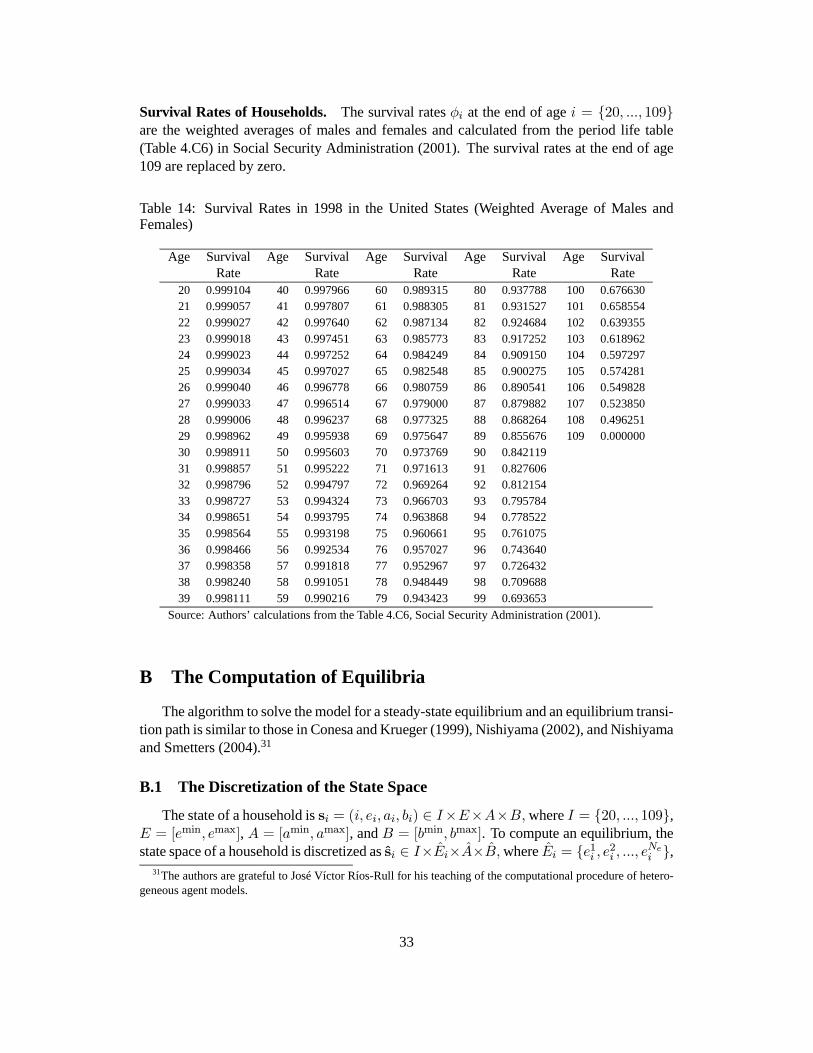
Survival Rates of Households. The survival rates φi at the end of age i = 20, ..., 109are the weighted averages of males and females and calculated from the period life table(Table 4.C6) in Social Security Administration (2001). The survival rates at the end of age109 are replaced by zero.

Table 14: Survival Rates in 1998 in the United States (Weighted Average of Males andFemales)

Age Survival Age Survival Age Survival Age Survival Age SurvivalRate Rate Rate Rate Rate

20 0.999104 40 0.997966 60 0.989315 80 0.937788 100 0.67663021 0.999057 41 0.997807 61 0.988305 81 0.931527 101 0.65855422 0.999027 42 0.997640 62 0.987134 82 0.924684 102 0.63935523 0.999018 43 0.997451 63 0.985773 83 0.917252 103 0.61896224 0.999023 44 0.997252 64 0.984249 84 0.909150 104 0.59729725 0.999034 45 0.997027 65 0.982548 85 0.900275 105 0.57428126 0.999040 46 0.996778 66 0.980759 86 0.890541 106 0.54982827 0.999033 47 0.996514 67 0.979000 87 0.879882 107 0.52385028 0.999006 48 0.996237 68 0.977325 88 0.868264 108 0.49625129 0.998962 49 0.995938 69 0.975647 89 0.855676 109 0.00000030 0.998911 50 0.995603 70 0.973769 90 0.84211931 0.998857 51 0.995222 71 0.971613 91 0.82760632 0.998796 52 0.994797 72 0.969264 92 0.81215433 0.998727 53 0.994324 73 0.966703 93 0.79578434 0.998651 54 0.993795 74 0.963868 94 0.77852235 0.998564 55 0.993198 75 0.960661 95 0.76107536 0.998466 56 0.992534 76 0.957027 96 0.74364037 0.998358 57 0.991818 77 0.952967 97 0.72643238 0.998240 58 0.991051 78 0.948449 98 0.70968839 0.998111 59 0.990216 79 0.943423 99 0.693653

Source: Authors’ calculations from the Table 4.C6, Social Security Administration (2001).

B The Computation of Equilibria

The algorithm to solve the model for a steady-state equilibrium and an equilibrium transi-tion path is similar to those in Conesa and Krueger (1999), Nishiyama (2002), and Nishiyamaand Smetters (2004).31

B.1 The Discretization of the State Space

The state of a household is si = (i, ei, ai, bi) ∈ I×E×A×B,where I = 20, ..., 109,E = [emin, emax], A = [amin, amax], and B = [bmin, bmax]. To compute an equilibrium, thestate space of a household is discretized as si ∈ I×Ei×A×B,where Ei = e1i , e2i , ..., eNei ,

31The authors are grateful to José Víctor Ríos-Rull for his teaching of the computational procedure of hetero-geneous agent models.

33

A = a1, a2, ..., aNa, and B = b1, b2, ..., bNb. For all these discrete points, the modelcomputes the optimal decision of households, d(si,St;Ψt) = (ci (.) , hi (.) , ai+1 (.)) ∈(0, cmax]× [0, hmaxi ]×A, the marginal values, ∂

∂av(si,St;Ψt) and ∂∂bv(si,St;Ψt), and the

values v(si,St;Ψt), given the expected factor prices and policy variables.32

To find the optimal end-of-period wealth, the model uses the Euler equation and bilinearinterpolation (with respect to a and b) of marginal values at the beginning of the next period.33

In a heterogeneous-agent economy, Ne, Na, and Nb are 8, 57, and 8, respectively. In arepresentative-agent economy, the numbers of grid points are 1, 61, and 6, respectively.34

B.2 A Steady-State Equilibrium

The algorithm to compute a steady-state equilibrium is as follows. LetΨ denote the time-invariant government policy ruleΨ = (WLS,WG, CG, τI(.), τP (.), τC , trSS (si), trLS (si)).

1. Set the initial values of factor prices (r0, w0), accidental bequests q0, the policy vari-ables (W 0

LS, C0G, τ

0C), and the parameters ϕ0I ,ϕ

0SS of policy functions (τI(.), trSS (si))

if these are determined endogenously.35

2. GivenΩ0 = (r0, w0, q0,W 0LS , C

0G, τ

0C ,ϕ

0I ,ϕ

0SS), find the decision rule of a household

d(si;Ψ,Ω0) for all si ∈ I × Ei × A× B.36

(a) For age i = 109, find the decision rule d(s109;Ψ,Ω0). Since the survival rateφ109 = 0, the end-of-period wealth ai+1(s109; .) = 0 for all s109. Compute con-sumption and working hours (ci(s109; .), hi(s109; .)) and, then, marginal values∂∂av(s109;Ψ,Ω

0) and values v(s109;Ψ,Ω0) for all s109.37

(b) For age i = 108, ..., 20, find the decision rule d(si;Ψ,Ω0), marginal values∂∂av(si;Ψ,Ω

0), and values v(si;Ψ,Ω0) for all si, using ∂∂av(si+1;Ψ,Ω

0) and∂∂bv(si+1;Ψ,Ω

0) recursively.

i. Set the initial guess of a0i+1(si; .).32Because the marginal value with respect to historical earnings, ∂

∂bv(si,St;Ψt), is difficult to obtain analyt-

ically, it is approximated by (v(., bj+1,St;Ψt)− v(., bj ,St;Ψt))/(bj+1 − bj) where j = 1, 2, ..., Nb.

33The marginal values with respect to wealth, ∂∂av(si,St;Ψt), are used in the Euler equation to obtain optimal

savings, the marginal values with respect to historical earnings, ∂∂bv(si,St;Ψt), are used in the marginal rate of

substitution condition of consumption for leisure to obtain optimal working hours, and the values, v(si,St;Ψt),are used to calculate welfare changes measured by compensating and equivalent variations in wealth.

34The grid points on A and B are not equally spaced. In a heterogeneous-agent economy, A ranges from-$271,000 to $33,825,000 (in 2001 growth-adjusted dollars) and B ranges from $8,000 to $80,400. In arepresentative-agent economy, A and B range from -$333,000 to $1,573,000 and from $8,000 to $80,400, re-spectively.

35If we find the capital-labor ratio, both r and w are calculated from the given production function and depre-ciation rate. In this paper, the endogenous policy variables are CG and ϕSS in baseline economies, and τC , ϕI ,trLS (si), andWLS in policy experiments.

36In the steady-state economy, the decision rule of a household d(si;Ψ,Ω0) is not a function of the aggregatestate of economy S = (x(si),WLS ,WG). The measure of household x(si) is determined uniquely by thesteady-state condition, and the government’s wealthWG is determined by the policy rule Ψ.

37The marginal value with respect to historical earnings, ∂∂bv(si;Ψ,Ω

0), is zero when i > 60 in this paper.

34

ii. Given a0i+1(si; .), compute (ci(si; .), hi(si; .)), using ∂∂bv(si+1;Ψ,Ω

0). Plugthese into the Euler equation with ∂

∂av(si+1;Ψ,Ω0).

iii. If the Euler error is sufficiently small, then stop. Otherwise, update a0i+1(si; .)and return to Step ii.

3. Find the steady-state measure of households x(si;Ω0) using the decision rule obtainedin Step 2. This computation is done forward from age 20 to age 109. Repeat this stepto iterate q for q1.

4. Compute new factor prices (r1, w1), accidental bequests q1, the policy variables (W 1LS,

C1G, τ1C), and the parameters ϕ1I ,ϕ

1SS of policy functions.

5. Compare Ω1 = (r1, w1, q1,W 1LS , C

1G, τ

1C ,ϕ

1I ,ϕ

1SS) with Ω0. If the difference is suf-

ficiently small, then stop. Otherwise, updateΩ0 and return to Step 2.

B.3 An Equilibrium Transition Path

Assume that the economy is in the initial steady state in period 0, and that the new policyscheduleΨ1, which was not expected in period 0, is announced at the beginning of period 1,where Ψ1 = WLS,t+1,WG,t+1, CG,t, τI,t (.) , τP,t (.) , τC,t, trSS,t (si) , trLS,t(si)∞t=1. LetS1 = (x1(si),WLS,1,WG,1) be the state of the economy at the beginning of period 1. Thestate of the economy S1 is usually equal to that of the initial steady state. The algorithmto compute a transition path to a new steady-state equilibrium (thereafter, final steady-stateequilibrium) is as follows.

1. Choose a sufficiently large number, T , such that the economy is said to reach the newsteady state within T periods. Set the initial guess, Ω01 = r0s , w0s , q0s ,W 0

LS,s, τ0C,s,

ϕ0I,sTs=1, on factor prices, accidental bequests, and the policy variables. Because thereare no aggregate productivity shocks in this model, a time series Ωt = r0s , w0s , q0s ,W 0LS,s, τ

0C,s,ϕ

0I,sTs=t is deterministic, and each household perfectly foreseesΩt based

on the information St in an equilibrium. Since St is in a household decision ruleonly to make the household expectΩt rationally, in the computation, we can avoid the“curse of dimensionality” by replacing d(si, St;Ψt) with d(si;Ψt,Ωt).

2. GivenWLS,T , find the final steady-state decision rule d(si;ΨT ,Ω0T ), marginal values,∂∂av(si;ΨT ,Ω

0T ), and values v(si;ΨT , Ω0T ) for all si ∈ I × Ei × A × B. (See the

algorithm for a steady-state equilibrium.)

3. For period t = T −1, T −2, ..., 1, based on the guess,Ω0t , find backward the decisionrule d(si;Ψt,Ω0t ), marginal values ∂

∂av(si;Ψt,Ω0t ), and values v(si;Ψt,Ω0t ) for all

si ∈ I × Ei × A× B, using the next period marginal values ∂∂av(si+1;Ψt+1,Ω

0t+1)

and values v(si+1;Ψt+1,Ω0t+1) recursively.

4. For period t = 1, 2, ..., T − 1, compute forward (r0t , w0t , q

0t ,W

0LS,t, τ

0C,t,ϕ

0I,t) and the

measure of households xt+1(si), using the decision rule d(si;Ψt,Ω0t ) obtained inStep 3 and using the state of economy St = (xt(si),WLS,t,WG,t) recursively.

35

5. Compare Ω1t with Ω0t . If the difference is sufficiently small, then stop. Otherwise,updateΩ0t and return to Step 2.

B.4 The Lump-Sum Redistribution Authority

When the Lump-Sum Redistribution Authority (LSRA) is assumed, the following com-putation is added to the iteration process.

1. For period t = T, T − 1, ..., 2, compute the lump-sum transfers to newborn house-holds trCV (s20;Ψt,Ω0t ) to make those households as well off as under the pre-reformeconomy.

(a) Set the initial value of lump-sum transfers trCV (s20;Ψt,Ω0t ) to newborn house-holds.

(b) Given trCV (s20;Ψt,Ω0t ), find the decision rule of newborn households d(s20;Ψt,Ω

0t ) and values v(s20;Ψt,Ω0t ).

(c) Find the compensating variation in wealth ∆trCV (s20;Ψt,Ω0t ) to make thosehouseholds indifferent from the baseline economy. (The initial wealth of new-born households is assumed to be zero since they do not receive any bequests.)If the absolute value of∆trCV (s20;Ψt,Ω0t ) is sufficiently small, then go to Step(d). Otherwise, update trCV (s20;Ψt,Ω0t ) by adding ∆trCV (s20;Ψt,Ω0t ) andreturn to Step (b).

(d) Set the lump-sum transfers trLS,t(s20) = trCV (s20;Ψt,Ω0t ) + ∆tr where an

additional lump-sum transfer ∆tr is precalculated, and find the decision rule ofnewborn households d(s20;Ψt,Ω0t ).

2. For period t = 1, compute the lump-sum transfers to all current households trCV (si;Ψt,Ω0t ) to make those households as much better off as the pre-reform economy. The pro-cedure is similar to Step 1. Set the lump-sum transfers trLS,1(si) = trCV (si;Ψt,Ω0t ).

3. Compute an additional lump-sum transfer ∆tr to newborn households so that the netpresent value of all transfers becomes zero. Compute the LSRA wealth, W 1

LS,tTt=1,which will be used to calculate national wealth. Recompute ∆tr and W 1

LS,tTt=1using new interest rates rtTt=1.

36

References

[1] Altig, David, Alan Auerbach, Laurence Kotlikoff, Kent Smetters, and Jan Walliser

(2001). “Simulating Fundamental Tax Reform in the United States.” American Economic

Review, 91, 3: 574-595.

[2] Auerbach, Alan (1996). “Tax Reform, Capital Allocation, Efficiency and Growth.” In

H. Aaron and W. Gale, Editors, Economic Effects of Fundamental Tax Reform. Brook-

ings Institution Press: Washington, D.C.

[3] Auerbach, Alan and Laurence Kotlikoff (1987). Dynamic Fiscal Policy, Cambridge Uni-

versity Press.

[4] Barro, Robert J. (1997). Macroeconomics (5th edition). The MIT Press: Cambridge,

Mass.

[5] Breyer, Friedrich (1989). “On the Intergenerational Pareto Efficiency on Pay-as-you-go

Financed Pension Systems.” Journal of Institutional and Theoretical Economics, 145, 4:

643-58.

[6] Conesa, Juan and Dirk Krueger (1999). “Social Security Reform with Heterogeneous

Agents.” Review of Economic Dynamics, 2, 4: 757-795.

[7] De Nardi, Mariacristina, Selahattin Imrohoroglu, and Thomas J. Sargent (1999). “Pro-

jected U.S. Demographics and Social Security.” Review of Economic Dynamics, 2, 3:

575-615.

[8] Diamond, Peter A. and Peter R. Orszag (2003). Saving Social Security: A Balanced

Approach. Brookings Institution Press: Washington, D.C.

[9] Feldstein, Martin (1995). “Would Privatizing Social Security Raise Economic Welfare?”

NBER Working Paper #5281.

[10] Floden, Martin and Jesper Lindé (2001). “Idiosyncratic Risk in the United States and

Sweden: Is There a Role for Government Insurance?” Review of Economic Dynamics,

4, 2: 406-37.

37

[11] Geanakoplos, John, Olivia S. Mitchell and Stephen P. Zeldes (1998). “Would a Pri-

vatized Social Security System Really Pay a Higher Rate of Return?” In D. Arnold,

M. Graetz, and A. Munnell, Editors, Framing the Social Security Debate: Values, Poli-

tics and Economics, 137-57. Brookings Institution Press: Washington, D.C.

[12] Gustman, Alan L. and Thomas L. Steinmeier (2001). “How Effective Is Redistribution

under the Social Security Benefit Formula?” Journal of Public Economics, 82, 1: 1-28

[13] Imrohoroglu, Ayse and Selahattin Imrohoroglu, and Douglas Joines (1995). “A Life

Cycle Analysis of Social Security.” Economic Theory, 6, 1: 83-114.

[14] Kotlikoff, Laurence J., Kent Smetters, Jan Walliser (2001). “Finding a Way Out of

America’s Demographic Dilemma.” NBER Working Paper 8258.

[15] Mariger, Randall (1999). “Social Security Privatization: What Are the Issues?” Na-

tional Tax Journal, 52, 4: 783-802

[16] Murphy, Kevin and Finis Welch (1998). “Perspectives on the Social Security Crisis and

Proposed Solutions.” American Economic Review, 88, 2: 142-50.

[17] Nishiyama, Shinichi (2002). “Bequests, Inter Vivos Transfers, and Wealth Distribu-

tion.” Review of Economic Dynamics, 5, 4: 892-931.

[18] Nishiyama, Shinichi (2004). “Analyzing an Aging Population—A Dynamic General

Equilibrium Approach.” Working Paper 2004-3, Congressional Budget Office.

[19] Nishiyama, Shinichi and Kent Smetters (2004). “Consumption Taxes and Economic

Efficiency with Idiosyncratic Wage Shocks.” Mimeo, Congressional Budget Office and

University of Pennsylvania

[20] Shiller, Robert (1999). “Social Security and Institutions for Intergenerational, Intra-

generational and International Risk Sharing.” Carnegie-Rochester Conference Series on

Public Policy, 50, 99: 165-204.

[21] Smetters, Kent (2005). “On the Potential for Pareto Improving Social Security Reform.”

Mimeo, The Wharton School.

[22] Social Security Administration (2001). Social Security Bulletin: Annual Statistical Sup-

plement, available at http://www.ssa.gov/statistics/supplement/2001/index.html.

38