Does Loan Loss Provision Timeliness Affect the … Liao...Does Loan Loss Provision Timeliness Affect the Accuracy, Informativeness, and Predictability of Analyst Provision Forecasts?

Does Loan Loss Provision Timeliness Affect the Accuracy,

Informativeness, and Predictability of Analyst Provision Forecasts?

Anne Beatty

[email protected]

Fisher College of Business

The Ohio State University

442 Fisher Hall

2100 Neil Avenue

Columbus, OH 43210

614-292-5418

Scott Liao

[email protected]

Rotman School of Management

University of Toronto

105 St. George Street

Toronto, ON M5S 3E6

416-946-8599

December 20, 2015

Abstract: We examine how the properties of equity analysts’ bank loan loss provision

forecasts differ with provision timeliness. We find that the accuracy of analyst provision

forecasts relative to time-series provision forecasts is more pronounced for banks with

more timely loan loss provisions. Consistent with the greater accuracy of analysts’

provision forecast for timely banks, we find that, controlling for time series provision

expectations, the equity market’s incremental response to analysts’ provision forecasts

beyond earnings forecasts is greater for banks with more timely loan loss provisions. We

further verify that the provision forecast is a better predictor of future non-performing

assets for banks with timely provisions. Finally, we find a greater ability of analysts’

provision forecasts to predict non-performing assets when analysts also provide a non-

performing asset forecast that is larger for timely than for untimely banks.

We thank seminar participants at the University of Arizona, University of Minnesota, University of

Alberta, Lancaster University, INSEAD Accounting Symposium, Andy Call and Shuping Chen for their

thoughtful comments and suggestions.

mailto:[email protected]

2

1. Introduction

Given the importance of accruals in predicting future earnings and cash flows

(e.g., Dechow, 1994; Barth et al., 2001), the scarcity of research examining analysts’

accruals forecasts seems surprising. We identify a setting where analysts issue explicit

accruals forecasts and examine the accuracy of these forecasts, whether these accrual

forecasts are incrementally useful to investors beyond earnings forecasts, and whether

these forecasts predict future performance. Specifically, we examine financial analysts’

explicit forecasts of loan loss provisions in banks, which Beatty and Liao (2014) argue is

banks’ most important accrual. 1 In addition, we consider whether analyst provision

forecasts reflect banks’ timeliness in loan loss provisioning by examining whether the

accuracy, usefulness and predictability of these forecasts depend on the timeliness of

banks’ provision accounting. We focus on the relation between banks’ timeliness in loan

loss provisioning, among other accounting properties, and analyst forecasts, because of

the important implication of provision timeliness in the current policy and accounting

standards debate, in particular the significant economic consequences of provision

timeliness at both the macro and micro levels.2

While the literature on sell-side analysts has established that analysts’ earnings

forecasts are more accurate than time-series (e.g., O’Brien, 1988), whether analysts’

1Beatty and Liao (2014) argue that relative to other accruals, the loan loss provision is large and explains

much of the variability in total accruals. Specifically, for years ended 2005-2012 the ratio of the mean of

the absolute values of the provision to that of total accruals is 56%, which is nearly twice the value of the

next largest accrual. Consistent with the relative magnitudes, the percentage of the variance of total

accruals explained by the provision of 34% is more than double the value of the accrual with the second

highest explanatory power.

2Both IASB and FASB are drafting the final standards requiring the adoption of expected loss models for

loan loss provision and expected loss models were once in the BASEL III discussions. In addition, Beatty

and Liao (2011) find that provision timeliness affects pro-cyclicality of lending and Bushman and Williams

(2012 and 2013) find that provision timeliness enhances market discipline in risk taking and affects

contribution to systemic risk.

3

forecasts of earnings components such as cash flows are more accurate than time-series is

under debate (e.g., Givoly et al., 2009). Nichols et al. (2009) argue that publicly traded

banks provide timelier loan loss provisions to mitigate information asymmetry. This

possibility could either advantage or disadvantage analysts relative to time-series

forecasts, because it is inherently more difficult to predict expected losses compared to

incurred losses. Therefore, to accurately predict provisions that are more timely, analysts

may need to conduct more research on the banks’ loan quality and predict borrowers’

future performance. In addition, based on the earnings forecast literature, it is not clear

whether analysts incorporate firms’ timely loss recognition when forecasting earnings

(e.g., Louis et al, 2008). Therefore, to shed light on this debate, we examine how

analysts’ relative provision forecast accuracy, measured as the difference between

provision forecast errors based on the analysts’ actual provision forecasts (i.e., absolute

values of the difference between reported provisions and the median of analyst provision

forecasts) versus predicted provisions based on time-series models (i.e., absolute values

of the difference between reported provisions and predicted provisions based on time-

series models), differs with the underlying timeliness of banks’ provision accounting.

Using a sample collected from the SNL database ranging from 2008 Q3 to 2013

Q3, we identify 3,928 bank-quarters (representing 246 individual banks) with analysts

forecasting both earnings and provisions. We find that provisions forecast errors are

smaller when calculated using the actual provision forecast compared to various time-

series models and that this differential is greater for banks with timely loan loss

provisions. This suggests not only that analyst provision forecasts contain additional

information about banks’ loan quality and banks’ overall information environments that

4

cannot be simply replicated using time-series models, but that this information advantage

is greater for banks that incorporate more expected losses in their loan loss provisions.

To evaluate the implications and usefulness of analyst provision forecasts for the

equity market, we examine the three-day cumulative abnormal equity market reaction on

earnings announcement dates., Previous research (e.g., Ahmed et al., 1999; Wahlen,

1994) examining the market response to unexpected provisions based on time series

models have found that the market differentially reacts to the provision component of

earnings although this differential reaction has been found to be either positive or

negative depending on the period studied. First we document an incremental negative

market response to the unexpected time-series provision component of earnings relative

to other earnings components consistent with the results in more recent studies. Next, we

find that, controlling for earnings surprises relative to earnings forecasts and for time-

series provision expectations, banks whose actual loan loss provisions exceed the

forecasted provisions experience a significant negative market return. This finding

supports the notion that analyst provision forecasts help market participants form

expectations of loan loss provisions beyond time-series models and therefore are

important for valuation purposes. We also examine whether the market reaction differs

for banks with more versus less timely loan loss provisioning. While we find no

difference in the reaction to earnings forecasts between these two types of banks, we find

that the market reacts more strongly to provision forecasts for banks with more timely

loan loss provisions. This reaction is consistent with the improved accuracy of analysts’

provision forecasts for banks with more timely loan loss provisions and suggests that

these forecasts serve better market expectations of banks’ loan losses.

5

To further support the notion that analysts incorporate banks’ provision timeliness

when forecasting provisions, we examine the association between analysts’ provision

forecasts and future non-performing assets to assess the predicting ability of loan loss

provision forecasts. By construction the reported loan loss provision should have a higher

association with future non-performing assets for more timely banks. However, it is not

obvious whether analysts will have the necessary information to predict these expected

future losses. We also examine the association between analysts’ provision forecast errors

and future non-performing assets to assess the extent to which analysts can predict

expected future losses. We find that provision forecasts are more positively associated

with future non-performing assets for banks with more timely provision accounting. This

suggests that analysts are able at least in part to predict expected future losses, however

we also find that provision forecast errors are associated with future non-performing

loans indicating that analysts forecasts do not fully incorporate the expected losses

reflected in the current period’s provision.

One potential mechanism that increases the timeliness of analysts’ provision

forecasts is nonperforming assets forecasts. In our sample, about 44% of banks covered

by analysts also receive forecasts of nonperforming assets. We argue that analysts that

also forecast nonperforming assets are better able to provide timely provision forecasts

because nonperforming assets are an important indicator for future losses (Beatty and

Liao, 2011; Bushman and Williams, 2012). Therefore, we further explore the ability of

provision forecasts to predict future non-performing assets by considering how these

associations differ when analysts also forecast non-performing assets. Consistent with our

6

expectations, we find a higher association between future non-performing assets and

analyst provision forecasts in the presence of non-performing asset forecasts.

While descriptive in nature, our findings contribute to two literatures. First, our

study adds to the large body of literature on sell-side analyst forecasts. We know very

little from the literature about whether analysts engage in accruals forecasts. While Call

et al. (2009) argue that analysts provide specific estimates of accounts receivables,

accounts payables, inventories and depreciation to derive estimates of cash flow,

evidence of whether analysts explicitly provide these forecasts to investors and of the

information content of accruals forecasts is lacking in the existing literature. We add to

this literature by showing that provision forecasts contain useful information that assists

market participants in forming expectations of a bank’s loan loss provision. We further

add to this literature by showing that analysts attempt to incorporate banks’ accounting

practices, i.e., timely loss recognition, in their accrual forecasts, which enables analysts to

outperform time-series models. While the provision forecasts do not completely predict

future losses, we show that analysts research additional information including

nonperforming assets to achieve more timely provision forecasts.

Our study also sheds light on the banking accounting literature. While the loan

loss provision is the most important bank accrual, very little is known about how the

equity market forms expectations about provisions and whether and how information

intermediaries such as financial analysts disseminate provision information. We add to

this literature by documenting that, beyond the provision component of earnings that is

included in analysts’ earnings forecasts, analysts make explicit provision forecasts that

are informative to the market and to predicting future non-performing assets. We further

7

find that the analysts’ provision forecasts are more accurate and more informative to the

market and in predicting future non-performing assets when loan loss provision

accounting is more timely.

The rest of the paper is organized as follows. In section 2, we discuss the related

literature and develop predictions on the determinants and consequences of loan loss

provision forecasts. We describe research methodology in section 3. In section 4, we

present sample descriptive statistics, empirical results and additional analyses. Section 5

concludes the paper.

2. Literature Review and Hypothesis Development

2.1. Loan Loss Provision Forecasts

While analysts do not provide explicit accruals forecasts for non-financial firms,

they provide forecasts for loan loss provisions for banks. Because the loan loss provision

is the most important accrual for banks and because of its significant economic

consequences to the overall economy (Beatty and Liao, 2014), an examination of loan

loss provision forecasts has the potential to expand the literature on sell-side financial

analysts, which has not examined explicit accruals forecasts.

Call et al. (2009) argue that when analysts forecast individual components of

earnings, they are likely to adopt a structured approach that includes analyses of a full set

of financial statements, thereby imposing greater forecasting discipline. Similar to

arguments made in Call et al. (2013) about forecasts of individual earnings components,

we argue that when forecasting provisions, analysts need to further understand the bank’s

system for identifying, monitoring and addressing loan problems and predicting future

loan quality, which cannot be replicated using time-series models. Therefore, we expect

8

that the provision forecast errors calculated using actual forecasts should be lower in

magnitude than using predicted provisions based on time-series models.

Further, we expect that the superiority of analysts forecast over time-series

forecasts will depend on the extent to which the provision includes expected future losses

in addition to incurred losses. Based on the argument in Nichols et al. (2009) that

publicly traded banks provide timelier loan loss provisions to mitigate information

asymmetry, we expect that analysts provision forecast accuracy relative to time-series

models might differ for banks with more timely loan loss provision accounting. On the

one hand analysts forecasts can incorporate their expectation of future losses that are not

captured in the time-series models, while on the other hand provision accounting that is

not based on incurred losses could be more difficult for analysts to predict. This

ambiguity is consistent with the mixed findings in the literature on whether analysts

incorporate firms’ accounting conservatism when forecasting earnings. For example,

while Louis et al. (2008) find that analysts do not fully incorporate firms’ timely loss

recognition into earnings forecasts, Helbok and Walker (2004) suggest that analysts base

their earnings forecasts on firms’ accounting conservatism.

Based on these arguments our first hypothesis (stated in the null form) is:

H1: The accuracy of analysts provision forecasts relative to time-series provision

forecasts does not differ based on provision timeliness.

2.2. Market Reaction to Loan Loss Provision Forecasts

Although the loan loss provision negatively impacts reported earnings, previous

several studies conducted in the early 1990s find a positive reaction to unexpected

provisions. For example, examining the three-day returns centered on the earnings

9

announcement dates, Wahlen (1994) finds that the market reacts positively to unexpected

provisions and earnings at the earnings announcement date. Similarly, Griffin et al.

(1991) and Elliot et al. (1991) find a positive market reaction for banks’ additions to loan

loss provisions. They interpret this as evidence that increased provisions provides

credible signals about banks’ intentions and abilities to resolve bad debt issues. However,

Ryan (2007) states that the evidence since 1993 does not show a positive market reaction

to increases in loan loss provisions. For example, Ahmed et al. (1999) find that the

market values the provision negatively beyond valuation of the provision component of

earnings. If the market responds more to the provision component than to other earnings

components, then we would expect a negative reaction to the provision surprise beyond

the response to the earnings surprise in our sample period.

If analyst forecasts help market participants form expectations about the loan loss

provision component of earnings, then, following previous research, we argue that the

short-term market returns around earnings announcements may depend on provision

surprises, i.e., actual provision minus the analyst median forecast. However, the direction

of the market reaction is not entirely obvious based on the findings in the literature. For

industrial firms with analyst cash flow forecasts, DeFond and Hung (2003) find a

significant market response to cash flow forecast errors but no significant market

response to the accrual component of earnings forecast errors. If the market responds less

to the provision component of earnings than to other earnings components like non-

financial firms, then this would suggest a positive reaction to the provision surprise after

controlling for the earnings surprise.

Based on these arguments, our second hypothesis (stated in the null form) is:

10

H2: The equity market reactions to provision surprises calculated based on both time-

series models and analyst provision forecasts (i.e. provision – provision forecasts)

are not different from zero.

Ryan (2007) argues that the market reaction to loan loss provisions depends on

the provisioning timeliness with more timely losses being perceived by the market as bad

news about impending loan defaults. Consistent with this possibility, we expect a more

negative reaction to provision forecast surprises for banks with more timely loan loss

provision accounting.

Based on these arguments our third hypothesis (stated in the null form) is:

H3: The equity market reaction to provision surprises (i.e. provision – provision

forecasts) does not differ based on provision timeliness.

2.3. Non-performing Assets Forecasts

To support the notion that analysts incorporate forward looking information in

provision forecasts when the covered banks are more timely in reporting loan losses, we

explore the predictive ability of loan loss provision forecasts by examining the

association between analysts’ provision forecasts and future non-performing assets. If the

provision forecasts reflect forward looking news about expected future losses, then we

expect the provision forecasts to be more positively associated with future non-

performing assets for banks with more timely provision accounting. However, because of

the inherent difficulty of incorporating forward-looking information in provision

forecasts, we expect analysts may not fully incorporate forward-looking information.

Therefore, we expect provision surprises (i.e., actual reported provisions minus analyst

forecasts) to also contain information about future losses, i.e., future nonperforming

assets especially for timely banks.

11

We further contend that, to better incorporate forward looking nonperforming

assets into provision forecasts, analysts may need to conduct more research on banks’

systems for managing problem loans and understanding the evolution of nonperforming

loans. We argue that analysts that also provide non-performing asset forecasts are more

likely to have conducted such research. Accordingly, we explore the ability of provision

forecasts to predict future non-performing assets by considering how these associations

differ when analysts also forecast non-performing assets. We expect that when analysts

forecast non-performing loans, their provision forecasts are more likely to reflect future

loan losses for banks with timely provisions. However, it is unclear whether the same is

true for banks with untimely provisions, since the analysts may want to minimize the

forecast error rather than best predict future loan losses.

Based on these arguments our fourth and fifth hypotheses (stated in the null form)

are:

H4: The ability of analyst provision forecasts to predict future non-performing loans

does not differ based on provision timeliness.

H5: The ability of analyst provision forecasts to predict future non-performing loans

in the presence of non-performing asset forecasts does not differ based on

provision timeliness.

3. Research Methodology

3.1 Equity Analysts’ Provision Forecasts vs. Time-Series Provision Forecasts

To explore whether analyst provision forecasts provide sophisticated information

that cannot be replicated by investors using publicly available information, we first

examine whether analyst provision forecasts are more accurate in predicting loan loss

provisions than various time-series models and whether provision timeliness affects this

12

difference in accuracy. Specifically, we compare the forecast errors calculated using

actual analyst provision forecasts to forecast errors using predicted values based on

various time-series models.

The first time-series model we consider is an AR1 time-series model (1):

Provisiont = 0 + 1Provisiont-1 + t. (1)

Based on Beatty and Liao (2011), the second time-series model (2) that we consider

includes other backward looking information including past non-performing loans,

lagged earnings before provision and Tier 1 capital ratio in addition to last quarter

provisions.

LLPt = 0+1NPLt-2 +2NPLt-1+3TIER1t-1+4*EBPt-1 +5LLPt-1 +t, (2)

where

LLP: Loan loss provision (COMPUSTAT “pllq”) divided by lagged total assets”).

NPL: Change in non-performing loans (COMPUSTAT “npatq”) divided by

lagged total assets (COMPUSTAT “atq”).

TIER1: The tier one risk-adjusted capital ratio (COMPUSTAT “capr1q”).

EBP: Earnings before loan loss provision, defined as (COMPUTAT “ibq” plus

COMPUSTAT “pllq”, scaled by lagged COMPUSTAT “atq”).

Specifically, we use the estimated coefficients from these time-series regressions

using the past 20 quarters before the quarter in question to calculate the predicted

provision for the current quarter.3 In an alternative model, we also allow the time-series

prediction model to include forward-looking information NPLt+1, one quarter ahead

change in nonperforming assets, as an explanatory variable.

3 We also replace the previous quarter provisions with four-quarter lagged provisions or add macro-

variables in alternative time-series models. All results continue to hold.

13

We then compare the forecast errors based on analyst forecasts versus these three

time-series models depending on the bank’s timeliness in recognizing provision using the

following model (3).

Inaccuracyt = β0 + β1Untimelyt + β2SIZEt-1+ β3NPLt-1 + β4*TIER1t-1 + β5EBPt-1

+ β6Charge-Offt-1 + β7LOANt-1 + β8Q4t +t,, (3)

where

Inaccuracy: absolute value of LLPSurprise minus the absolute value of either LLP-

PLLP1, LLP-PLLP2or LLP-PLLP3.

LLPSurprise: the actual reported provision (COMPUSTAT “pllq”), scaled by lagged

total assets (COMPUSTAT “atq”) minus LLPForecast.

LLP-PLLP1: the actual reported provision (COMPUSTAT “pllq”) minus the

predicted value of provision based on the AR1 time-series model (1)

using the data from past 20 quarters on a rolling basis, scaled by lagged

total assets (COMPUSTAT “atq”).


predicted value of provision based on a time-series model (2), where the

explanatory variables include one-quarter lagged provision, NPLt-1,

NPLt-2, one-quarter lagged EBP and TIER1, scaled by lagged total

assets (COMPUSTAT “atq”).


predicted value of provision based on a time-series model where the

explanatory variables include lagged provisions, NPLt-1, NPLt-2,

NPLt+1, one-quarter lagged EBP, TIER1 and one-quarter ahead , scaled

by lagged total assets (COMPUSTAT “atq”).

Untimely : An indicator variable equal to one when Timeliness is below the sample

median, zero otherwise.

Timeliness: Measured as the adjusted R-squared of EQ(a) minus adjusted R-squared

of EQ(b) using the data from the past 20 quarters on a rolling basis,

where

EQ(a): LLPt = 0 + 1NPLt+1 + 2NPLt+3NPLt-1 + 4NPLt-2+5TIER1t

+ 6*EBPt + t

EQ(b): LLPt = 0 + 1NPLt-1 + 2NPLt-2+3TIER1t + 4*EBPt + t

LLP: Loan loss provision (COMPUSTAT “pllq”) divided by lagged total

assets (COMPUSTAT “atq”);

NPL: Change in non-performing loans (COMPUSTAT “npatq”) divided by

lagged total assets (COMPUSTAT “atq”);

TIER1: The tier one risk-adjusted capital ratio (COMPUSTAT “capr1q”);



Charge-Off: net charge offs (COMPUSTAT “ncoq”) scaled by lagged total assets.

14

LOAN: Total loans (COMPUSTAT “lntalq”) scaled by total assets.

Q4: An indicator variable equal to 1 for the 4th fiscal quarter.

In Model (3), in addition to the independent variable of interest (Untimely) that

captures the timeliness of loan loss provisioning, we also control for bank characteristics

that potentially affect analyst forecasts without specific predictions. Based on H1, we

expect the coefficient on Untimely to differ from zero..

3.2 Market Reactions to Provision Forecast Errors at Earnings Announcements

To test whether market participants form provision expectations based on

analysts’ provision forecasts, we use the following OLS estimation (4) where we regress

3-day (-1, +1) market adjusted cumulative returns around earnings announcements on

both earnings surprises and provision surprises calculated using analyst median earnings

and provision forecasts.

RETURNt = β0 + β1*NISurpriset + β2*LLPSurpriset + β3*∆NIt + β4* LLP-PLLP1 +

β5*∆SIZEt + β6*∆NPLt+ β7*∆TIER1t+ β8*Q4t+ εt (4)

where

RETURN: 3-day (-1, 1) cumulative abnormal returns around earnings

announcements, where abnormal returns is measured as bank daily return

minus bank sector equal weighted return.

NIForecast: the median analyst net income forecast, scaled by lagged total assets

(COMPUSTAT “atq”).

LLPForecast: the median analyst provision forecast, scaled by lagged total assets


NISurprise: the actual reported net income (COMPUSTAT”niq”), scaled by lagged

total assets (COMPUSTAT “atq”) minus NIForecast.


total assets (COMPUSTAT “atq”) minus LLPForecast.


predicted value of provision based on the AR1 time-series model using

the data from past 20 quarters on a rolling basis, scaled by lagged total

assets (COMPUSTAT “atq”).

∆NI: change in net income (COMPUSTAT”niq”) scaled by lagged total assets


∆SIZE: change in bank size, where bank size is measured as the natural log of

total asset (COMPUSTAT “atq”).

15

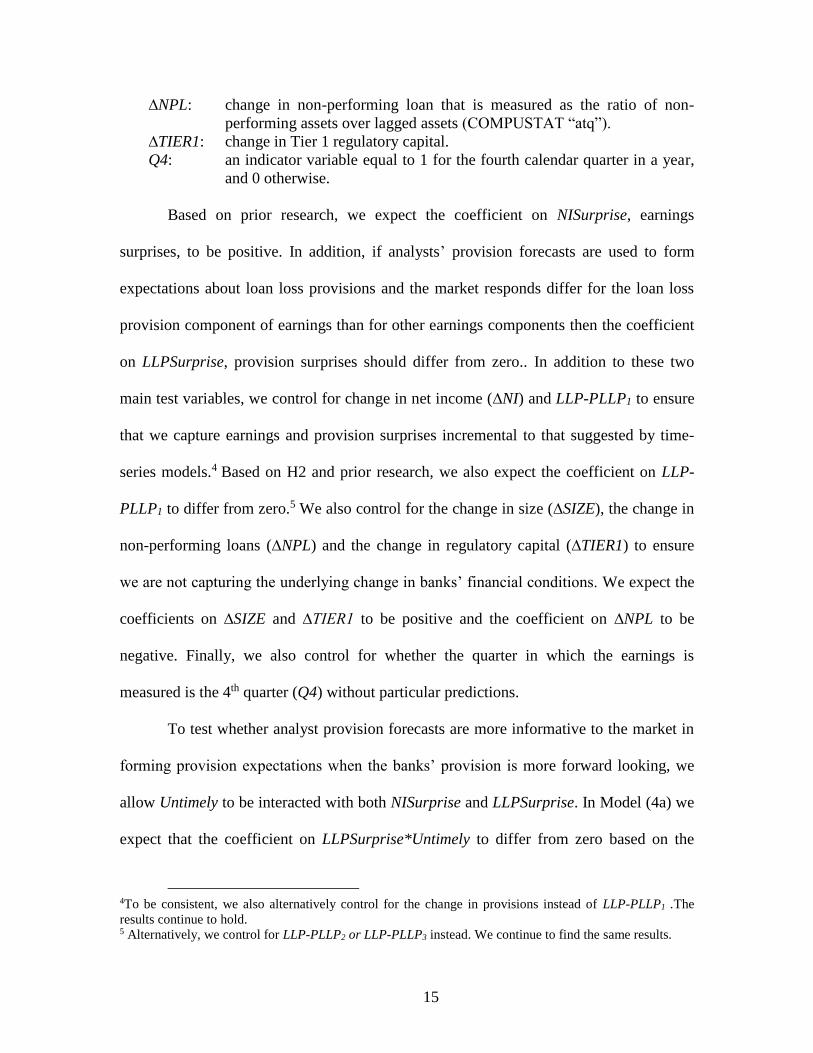
∆NPL: change in non-performing loan that is measured as the ratio of non-

performing assets over lagged assets (COMPUSTAT “atq”).

∆TIER1: change in Tier 1 regulatory capital.

Q4: an indicator variable equal to 1 for the fourth calendar quarter in a year,

and 0 otherwise.

Based on prior research, we expect the coefficient on NISurprise, earnings

surprises, to be positive. In addition, if analysts’ provision forecasts are used to form

expectations about loan loss provisions and the market responds differ for the loan loss

provision component of earnings than for other earnings components then the coefficient

on LLPSurprise, provision surprises should differ from zero.. In addition to these two

main test variables, we control for change in net income (∆NI) and LLP-PLLP1 to ensure

that we capture earnings and provision surprises incremental to that suggested by time-

series models.4 Based on H2 and prior research, we also expect the coefficient on LLP-

PLLP1 to differ from zero.5 We also control for the change in size (∆SIZE), the change in

non-performing loans (∆NPL) and the change in regulatory capital (∆TIER1) to ensure

we are not capturing the underlying change in banks’ financial conditions. We expect the

coefficients on ∆SIZE and ∆TIER1 to be positive and the coefficient on ∆NPL to be

negative. Finally, we also control for whether the quarter in which the earnings is

measured is the 4th quarter (Q4) without particular predictions.

To test whether analyst provision forecasts are more informative to the market in

forming provision expectations when the banks’ provision is more forward looking, we

allow Untimely to be interacted with both NISurprise and LLPSurprise. In Model (4a) we

expect that the coefficient on LLPSurprise*Untimely to differ from zero based on the

4To be consistent, we also alternatively control for the change in provisions instead of LLP-PLLP1 .The

results continue to hold. 5 Alternatively, we control for LLP-PLLP2 or LLP-PLLP3 instead. We continue to find the same results.

16

argument that analyst forecasts are more informative of future losses when the bank is

more timely in recognizing loan losses, while we do not expect the coefficient on

NISurprise*Untimely to be significantly different from zero if the timeliness of the

provision does not affect the informativeness of the non-provision earnings components.

RETURNt = β0 + β1*Untimelyt + β2*NISurpriset + β3*LLPSurpriset +

β4*NISurprise*Untimelyt + β5*LLPSurprise*Untimelyt + β6*∆NIt +

β7* LLP-PLLP1t + β8*∆SIZEt + β9*∆NPLt+ β10*∆TIER1t+ β11*Q4t+ εt (4a)

3.3 Analysts Provision Forecasts and Future Non-performing Assets

To test whether analysts provision forecasts predict future non-performing assets

we estimate the following model (5):

NPLt-+1 = β0 + β1 LLPForecastt + β2 Untimelyt + β3 LLPForecast*Untimelyt

+ β4NPLt-1+ β5SIZEt +β6TIER1t-1+ β7Charge-offt-1 + β8EBPt-1 +

β9LOANt-1+ β10Q4t +t (5)

In Model (5), LLPForecast is measured as analyst provision forecasts scaled by lagged

total assets. We expect the coefficient on LLPForecast*Untimely to differ from zero if

the ability of analyst provision forecasts to predict future nonperforming assets differs for

timely versus untimely banks. We also control for bank characteristics that are likely to

affect future nonperforming loans without particular predictions. Other variables are

defined as above or as in Appendix A.

To examine how the associations between future non-performing loans and

provision forecasts differs in the presence of non-performing loan forecasts we estimate

Model (5) separately for banks with nonperforming loans forecasts versus without such

forecasts. We expect the coefficients on LLPForecast and on LLPForecast*Untimelyt to

differ for banks with nonperforming loan forecasts.

17

4. Samples and Findings

4.1 Samples and Databases

Our provision forecast information is acquired from SNL, which contains both

analyst provision and net income forecasts for banks starting from the third quarter of

2008. We require the bank to be publicly traded and covered by CRSP for market

reaction analyses. Finally, other bank characteristics are acquired from COMPUSTAT.

Based on the intersection of these databases and the requirement of non-missing values

for test and control variables, we end up with 3,928 bank-quarters with provision

forecasts (representing 246 banks) for the period from the third quarter of 2008 through

the third quarter of 2013.

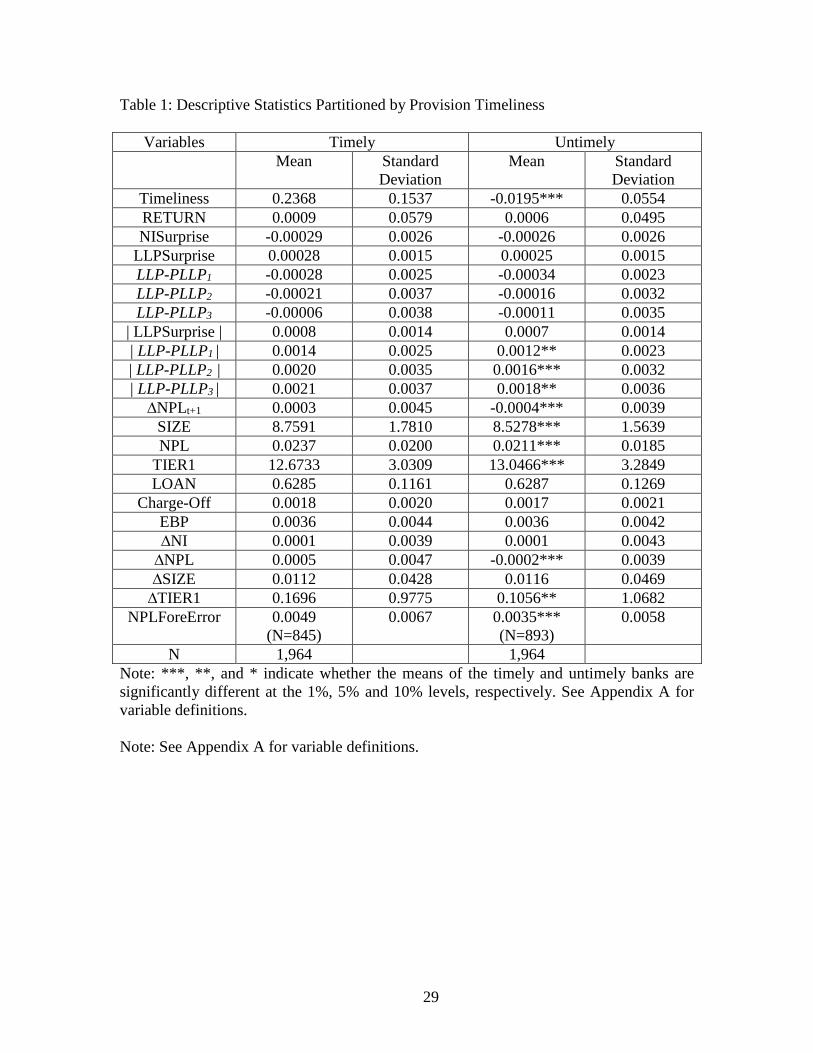
Table 1 shows bank characteristics and our main variables partitioned by

provision timeliness. We find that on average banks’ earnings are lower than the forecasts

while banks’ provisions tend to be higher than the analyst forecast. We also find that

consistent with our expectation, for both timely and untimely banks, analyst provision

forecast errors (0.0008 and 0.0007, respectively) are lower than forecast errors based on

time-series (0.0014 and 0.0012 for the first time series model, 0.0020, and 0.0016 for the

second time series model, and 0.0021 and 0.0018, respectively, for the third time series

model) at the 1% significance level (the test is not tabulated), suggesting that analyst

provision forecasts contain useful information beyond what can be learned from time-

series models. We also find that based on all three time series models, provision forecast

errors are larger for timely banks than untimely banks, suggesting that it is more difficult

to predict the provision when the bank’s provisioning is more timely. Further, we find

that timely banks are larger, have more nonperforming assets, and have lower regulatory

18

capital compared to untimely banks. We present Pearson correlations among test and

control variables in Table 2. We find that consistent with our expectation, the 3-day

abnormal returns around earnings announcement are positively correlated with

NISurprise while negatively correlated with LLPSurprise.

4.2 Empirical Findings

4.2.1 Analysts versus Time-Series Provision Forecasts

In Table 3 we explore whether the advantage of analyst provision forecasts over

time-series models depends on banks’ timeliness of loan loss provisioning. We find that

provision forecast relative inaccuracy, measured as |LLPSurprise| - |LLP-PLLP1|,

|LLPSurprise| - |LLP-PLLP2|, or |LLPSurprise| - |LLP-PLLP3|, is significantly higher for

banks with less timely loan loss recognition, significant at the 5% for time-series model

1) and 1% levels for time-series models 2) and 3). This finding suggests that analysts

have a comparative advantage forecasting provisions when the underlying provision is

timely. Analysts’ forecast advantage for timely banks holds for all three time series

models we consider and interestingly is the smallest for the simplest AR1 time series

model.

4.2.2 Market Reaction to Provision Forecasts

Table 4 presents the results of our analysis of the market reactions to provisions

and earnings announcements. The findings in Panel A Model 1 are consistent with recent

findings in prior studies that the market reacts more strongly to the unexpected loan loss

provision component of earnings than to other earnings components. In model 2 where

the earnings surprise based on analyst earnings forecasts (NISurprise) is added there is a

significant market reaction to the analyst forecast surprise and the market reaction to the

19

time-series earnings forecast surprise becomes insignificant. The time-series provision

forecast surprise remains significant however suggesting that the analyst earnings

forecast surprise does not capture all of the time-series information about the provision.

In model 3 where the analyst provision surprise (LLPSurprise) is also added, there is a

significant market reaction to the analyst provision forecast surprise and the market

reaction to the time-series provision forecast surprise becomes insignificant. This

suggests that analyst provision forecast provides information to the market beyond what

is provided by either the analyst earnings forecast or the time-series provision forecast.

This indicates that separately forecasting the provision provides useful information

beyond what is learned from the provision component of earnings.

In Panel B we extend our Panel A analysis to consider whether our findings differ

based on banks’ provision timeliness. In model 1 we find limited evidence that provision

timeliness affects the markets’ reaction to either time-series earnings or provision

surprises. When we add analyst forecast surprises in models (2) and (3) and allow the

coefficients on the earnings and provision surprises to differ for banks with more and less

timely provision accounting, we find no difference in the coefficient on earnings forecast

errors across this partition, but we find a significantly larger negative response to the

provision forecast errors for more timely versus less timely banks. These results suggest

that.analysts forecast surprises for banks with timely loan loss provisioning are

informative to the market but those for banks with untimely provisions are not.

4.2.3 Analysts Provision Forecasts and Future Non-performing Assets

The first column of Table 5 provides the results of our analysis of the association

between future non-performing assets and analysts’ loan loss provision forecasts.

20

Consistent with the accuracy and usefulness of the provision forecasts being greater for

banks with more timely loss recognition, we find that the provision forecasts are

positively associated with future non-performing assets for banks with timely provision

accounting and that the association is significantly lower for those with less timely

provisions. This suggests that analysts attempt to map provision forecasts into future

performance when providing forecasts for timely banks.

To further investigate whether analysts fully incorporate the loan loss provision

timeliness in capturing future performance, we examine whether provision surprises

predict one-quarter ahead nonperforming loans. In the second column of Table 5, we find

that when the provision is timely, provision surprises are better able to predict future

nonperforming loans, suggesting that despite their efforts to incorporate future

performance in provision forecasts, analysts cannot fully incorporate the expected losses

recognized in the provision. This again reflects the inherent difficulty of forecasting

forward looking provisions.

In Panel A of Table 6, we examine whether the timeliness of analyst provision

forecasts depend on the presence of nonperforming loan forecasts using the overall

sample. We allow these coefficients on LLPForecast in Model (5) to also vary based on

the existence of a non-performing asset forecasts. We find that, relative to untimely

banks, the association between provision forecasts for timely banks and next period’s

non-performing assets becomes stronger in the presence of a non-performing asset

forecast. This result suggests that analysts can improve their timeliness in provision

forecasts for timely banks by understanding the factors that affect nonperforming loans,

including banks’ systems for identifying, addressing and monitoring loan problems. This

21

finding may also suggest that analysts do not choose to incorporate those expectations

into their forecasts for untimely banks that only provide for incurred losses. The lower

association between future non-performing loans and provision forecasts for untimely

banks is consistent with the market finding those forecasts less informative.

4.3 Additional Analyses and Robustness Checks

The presence of nonperforming asset forecasts may be an endogenous choice,

which may affect the inference of results in the previous section. To address this issue,

we employ a propensity score matching approach. In the first stage model of predicting

nonperforming asset forecasts, we use the following logistic model (6):

NonPerfForecast = β0 + β1LOAN_REt-1 + β2LOAN_COMt-1+ β3NPLt-1 + β4SIZEt-1 +

β5TIER1t-1 + β6EBPt-1 + β7Charge-Offt-1 + β8Q4t +t,, (6)

where

NonPerForecast :An indicator variable equal to one for banks with nonperforming

loan forecasts. LOAN_RE : Measured as the ratio of real estate loans divided by total loans.

LOAN_COM : Measured as the ratio of commercial loans divided by total loans.

In Panel B of Table 6, we find the coefficients on LOAN_RE and LOAN_COM to

be positive suggesting that the demand for nonperforming loan forecasts is higher for

more heterogeneous loans. We also find that this nonperforming loan forecast is more

likely for larger firms. Based on the propensity score calculated using this prediction

model, we form a matched sample and conduct the estimation of the same model (5). In

the last two columns of Table 6, we find that, based on the matched sample, the results

continue to hold, suggesting that selection bias is not likely driving our findings. That is,

analyst provision forecasts are more likely to predict future nonperforming loans in the

presence of nonperforming loan forecasts.

22

As an additional analysis on the usefulness of analyst provision forecasts, we also

examine whether the trading volume is affected by analyst provision forecasts. In

untabulated results, we find that around the earnings and provision announcement dates,

abnormal trading volume increases with both earnings forecast errors and provision

forecast errors, further suggestive of the usefulness of analyst provision forecasts in

forming market expectations. Further, in the market return analysis, the results also

continue to hold when RETURN is defined alternatively using the market equal or value

weighted return in CRSP as the benchmark as opposed to using the bank sector average

return as the benchmark. We also follow prior research by scaling variables in the market

reaction analysis using market value of equity instead of total assets. The results continue

to hold. Finally, we define RETURN using 5-day (-2, 2) cumulative abnormal returns, and

the results continue to hold.

5. Conclusion

In this paper, we study analyst loan loss provision forecasts, which have not been

explored in previous research. We first examine the relative accuracy of analyst provision

forecasts relative to three time-series provision forecast models and find that analysts are

more accurate for banks with more timely provisioning relative to those with less timely

provisioning.

We next examine the information content of provision forecasts by studying the

market returns to earnings and provisions announcements for both time-series and analyst

forecasts. We find that the 3-day abnormal returns increase with earnings surprises and

decrease with provision surprises based on time-series models, indicating that the market

applies a greater multiple to the provision component of earnings than to other earnings

23

components. The time-series provision surprise continues to be associated with abnormal

returns when we add analyst earnings surprise to the model but becomes insignificant

when we include analyst provision surprise. This suggests that the provision forecasts

provide information that cannot be gleaned from either the analyst earnings forecast or

the time-series provision forecast.

When we examine how the market response varies with provision timeliness, we

find limited evidence that the response to time-series forecasts of either earnings or the

provision differs by timeliness. The market response to analyst earnings forecast errors

similarly does not differ based on provision timeliness, but the response to the analyst

provision forecast errors is more negative for more timely versus less timely banks. These

results suggest that analyst provision forecasts contain more forward looking information

as a benchmark for provisions.

To further investigate whether analysts’ forecasts incorporate the expected losses

recognized in the loan loss provision, we examine the association between future non-

performing assets and analyst loan loss provision forecasts. We find that provision

forecasts are positively associated with future non-performing assets for banks with

timely loss recognition, but that the association is much lower for those with less timely

provisions. We further find that analyst provision surprises are also more positively

associated with future non-performing assets for timely banks. These results are

consistent with the accuracy and usefulness of the prevision forecasts being greater for

banks with more timely loss recognition, but also with the forecast not fully incorporating

the expected losses recognized in the provision.

24

Our study makes two major contributions to the literature. We add to the literature

on sell-side financial analysts by expanding our understanding of the properties of analyst

accruals forecasts, which have largely been ignored in the analyst literature. In addition,

we expand the literature on loan loss provisions by providing a new perspective on how

and whether analyst provision forecasts form market expectations about provisions and

on how provision timeliness affects the markets’ response to those forecasts. We also

expand our understanding of the timely provision recognition practice in relation to

analyst provision forecasts.

25

Reference

Ahmed, A. S. Thomas, and C. Takeda. 1999. Bank loan loss provisions: A reexamination

of capital management, earnings management & signaling effects. Journal of Accounting

& Economics 28, 1-26.

Barth, M. E., D. Cram, and K. Nelson. 2001. Accruals and the prediction of future cash

flows. The Accounting Review 76: 27–58.

Beatty, A., and S. Liao. 2011. Do delays in expected loss recognition affect banks’

willingness to lend? Journal of Accounting and Economics 52: 1-20.

Beatty, A., and S. Liao. 2014. Financial Accounting in the Banking Industry: A review of

the empirical literature. Journal of Accounting and Economics 58: 339-383.

Burgstahler, D., and I. Dichev. 1997. Earnings management to avoid earnings decreases

and losses. Journal of Accounting and Economics 24: 99-126.

Bushman, R., and C. Williams. 2012. Accounting discretion, loan loss provisioning, and

discipline of banks’ risk-taking. Journal of Accounting and Economics 54: 1-18.

Bushman, R., and C. Williams. 2013. Delayed expected loss recognition and the risk

profile of banks. Working Paper.

Call, A. C., S. Chen, and Y. H. Tong. 2009. Are analysts’ earnings forecasts more

accurate when accompanied by cash flow forecasts? Review of Accounting Studies 14

(2–3): 358–91.

Call, A, S. Chen and Y. Tong. 2013. Are analysts’ cash flow forecasts naıve extensions

of theirown earnings forecasts? Contemporary Accounting Research 30: 438-465.

Dechow, P. M. 1994. Accounting earnings and cash flows as measures of firm

performance: The role of accounting accruals. Journal of Accounting and Economics 18

(1): 3–42.

DeFond, M., and M. Hung. 2003. An empirical analysis of analysts’ cash flow forecasts.

Journal of Accounting and Economics 35: 73–100.

Elliot, J., D. Hanna, W. Shaw. 1991. The evaluation by the financial markets of changes

in bank loan loss reserve levels. The Accounting Review 66: 847-861.

Givoly, D., C. Hayn, and R. Lehavy. 2009. The quality of analysts’ cash flow forecasts.

The Accounting Review 84: 1877–911.

Grffin, P., and A. Wallch, and J. Samoa. 1991. Latin American lending by major U.S.

banks: The effects of disclosures about nonaccrual: Loans and loan loss provisions. The

Accounting Review 66, 830-846.

26

Helbok, G., M Walker. 2004. On the nature and rationality of analysts’ forecasts under

earnings conservatism. British Accounting Review 36: 45-77.

Liu, C., S. Ryan, and J. Wahlen. 1997. Differential valuation implications of loan loss

provisions across banks and fiscal quarters. The Accounting Review 72: 133-146.

Louis, H., T. Lys and A. Sun. 2008. Conservatism and analyst earnings forecast bias.

Working Paper, Penn State University.

McInnis, J. and D. Collins. 2011. The effect of cash flow forecasts on accrual quality and

benchmark beating. Journal of Accounting and Economics 51: 219–39.

Mohanram, P. 2014. Analysts’ cash flow forecasts and the decline of the accruals

anomaly. Contemporary Accounting Research, forthcoming.

O’Brien, P. C. 1988. Analysts’ forecasts as earnings expectations. Journal of Accounting

and Economics 10 (1): 53-83.

Ryan, S. 2007. Financial Instruments and Institutions: Accounting and Disclosure Rules,

second edition. John Wiley & Sons.

Wahlen, J. 1994. The nature of information in commercial bank loan loss disclosures.

The Accounting Review 69, 455-478.

27

Appendix A: Variable Definitions

Timeliness Measures:

Untimely: An indicator variable equal to one when Timeliness is below the sample

median, zero otherwise.

Timeliness: measured as the adjusted R-squared of EQ(a) minus adjusted R-squared of

EQ(b) using the data from the past 20 quarters on a rolling basis, where

EQ(a): LLPt = 0 + 1NPLt+1 + 2NPLt+3NPLt-1 + 4NPLt-2+5TIER1t +

6*EBPt + t

EQ(b): LLPt = 0 + 1NPLt-1 + 2NPLt-2+3TIER1t + 4*EBPt + t

LLP: Loan loss provision (COMPUSTAT “pllq”) divided by lagged total assets

(COMPUSTAT “atq”);

NPL: Change in non-performing loans (COMPUSTAT “npatq”) divided by lagged total

assets (COMPUSTAT “atq”);

TIER1: The tier one risk-adjusted capital ratio (COMPUSTAT “capr1q”);



Dependent and Test Variables:

RETURN: 3 day (-1, 1) cumulative abnormal returns around earnings announcements,

where abnormal returns is measured as bank daily return minus bank sector

equal weighted return.

NIForecast: the median analyst net income forecast, scaled by lagged total assets


LLPForecast: the median analyst provision forecast, scaled by lagged total assets


NISurprise: the actual reported net income (COMPUSTAT”niq”) , scaled by lagged

total assets (COMPUSTAT “atq”) minus NIForecast.


total assets (COMPUSTAT “atq”) minus LLPForecast

LLP-PLLP1: the actual reported provision (COMPUSTAT “pllq”) minus the predicted

value of provision based on the AR1 time-series model using the data from past 20

quarters on a rolling basis, scaled by lagged total assets (COMPUSTAT “atq”).


value of provision based on a time-series model, where the explanatory variables

include one-quarter lagged provision, NPLt-1, NPLt-2, one-quarter lagged EBP

and TIER1, scaled by lagged total assets (COMPUSTAT “atq”).


value of provision based on a time-series model where the explanatory variables

include lagged provisions, NPLt-1, NPLt-2, NPLt+1, one-quarter lagged EBP,

TIER1 and one-quarter ahead , scaled by lagged total assets (COMPUSTAT “atq”).

Inaccuracy: absolute value of LLPSurprise minus the absolute value of either LLP-

PLLP1, LLP-PLLP2 or LLP-PLLP3 .

28

Bank Characteristic Control Variables

SIZE: the natural log of lagged total asset (COMPUSTAT “atq”).

NPL: the lagged ratio of non-performing assets over total assets (COMPUSTAT “atq”).

TIER1: lagged tier one risk-adjusted capital ratio (COMPUSTAT “capr1q”);

LOAN: total loans (COMPUSTAT “lntalq”) scaled by total assets,.

Charge-Off: net charge offs (COMPUSTAT “ncoq”) scaled by lagged total assets.

EBP: the ratio of earnings before loan loss provision, defined as (COMPUTAT “ibq” plus


∆NI: change in net income (COMPUSTAT”niq”) scaled by lagged total assets


∆NPL: change in non-performing loan that is measured as the ratio of non-performing

assets over total assets (COMPUSTAT “atq”).

∆SIZE: change in bank size, where bank size is measured as the natural log of total asset


∆TIER1: change in Tier 1 regulatory capital.

Q4: an indicator equal to one for the fourth fiscal quarter in a year, zero otherwise.

29

Table 1: Descriptive Statistics Partitioned by Provision Timeliness

Variables Timely Untimely

Mean Standard

Deviation

Mean

Standard

Deviation

Timeliness 0.2368 0.1537 -0.0195*** 0.0554

RETURN 0.0009 0.0579 0.0006 0.0495

NISurprise -0.00029 0.0026 -0.00026 0.0026

LLPSurprise 0.00028 0.0015 0.00025 0.0015

LLP-PLLP1 -0.00028 0.0025 -0.00034 0.0023

LLP-PLLP2 -0.00021 0.0037 -0.00016 0.0032

LLP-PLLP3 -0.00006 0.0038 -0.00011 0.0035

| LLPSurprise | 0.0008 0.0014 0.0007 0.0014

| LLP-PLLP1 | 0.0014 0.0025 0.0012** 0.0023

| LLP-PLLP2 | 0.0020 0.0035 0.0016*** 0.0032

| LLP-PLLP3 | 0.0021 0.0037 0.0018** 0.0036

∆NPLt+1 0.0003 0.0045 -0.0004*** 0.0039

SIZE 8.7591 1.7810 8.5278*** 1.5639

NPL 0.0237 0.0200 0.0211*** 0.0185

TIER1 12.6733 3.0309 13.0466*** 3.2849

LOAN 0.6285 0.1161 0.6287 0.1269

Charge-Off 0.0018 0.0020 0.0017 0.0021

EBP 0.0036 0.0044 0.0036 0.0042

∆NI 0.0001 0.0039 0.0001 0.0043

∆NPL 0.0005 0.0047 -0.0002*** 0.0039

∆SIZE 0.0112 0.0428 0.0116 0.0469

∆TIER1 0.1696 0.9775 0.1056** 1.0682

NPLForeError 0.0049

(N=845)

0.0067 0.0035***

(N=893)

0.0058

N 1,964 1,964

Note: ***, **, and * indicate whether the means of the timely and untimely banks are

significantly different at the 1%, 5% and 10% levels, respectively. See Appendix A for

variable definitions.

Note: See Appendix A for variable definitions.

Table 2: Pearson Correlations (and p-values) among Main Variables (2) (3) (4) (5) (6) (7) (8) (9) (10) (11) (12) (13) (14) (15) (16)

Untimely

(1)

-0.003

(0.836)

0.007

(0.658)

-0.009

(0.564)

-0.022

(0.169)

-0.077

(0.001)

-0.069

(0.001)

-0.065

(0.001)

0.059

(0.001)

0.000

(0.956)

-0.023

(0.142)

-0.002

(0.903)

-0.002

(0.885)

-0.083

(0.001)

0.005

(0.765)

-0.031

(0.050)

RETURN

(2)

0.282

(0.001)

-0.268

(0.001)

-0.178

(0.001)

-0.040

(0.012)

-0.060

(0.001)

-0.017

(0.274)

0.014

(0.382)

0.008

(0.609)

-0.020

(0.200)

-0.001

(0.948)

0.182

(0.001)

-0.186

(0.001)

0.044

(0.006)

0.056

(0.001)

NI

Surprise (3)

-0.593 (0.001)

-0.529 (0.001)

-0.085 (0.001)

0.021 (0.194)

-0.145 (0.001)

0.136 (0.001)

-0.074 (0.001)

-0.168 (0.001)

0.102 (0.001)

0.583 (0.001)

-0.151 (0.001)

0.122 (0.001)

0.122 (0.001)

LLP_

Surprise (4)

0.809

(0.001)

0.157

(0.001)

-0.053

(0.001)

0.165

(0.001)

-0.103

(0.001)

0.147

(0.001)

0.166

(0.001)

-0.056

(0.002)

-0.317

(0.001)

0.207

(0.001)

-0.018

(0.270)

-0.091

(0.001)

| LLP_

Surprise |

(5)

0.063

(0.001)

-0.126

(0.001)

0.345

(0.001)

-0.103

(0.001)

0.200

(0.001)

0.322

(0.001)

-0.012

(0.001)

-0.229

(0.001)

0.115

(0.001)

-0.084

(0.001)

-0.054

(0.000)

∆NPLt+1

(6)

0.001

(0.959)

-0.192

(0.001)

-0.113

(0.001)

0.097

(0.001)

-0.061

(0.001)

-0.020

(0.201)

-0.009

(0.569)

0.263

(0.001)

0.065

(0.001)

0.078

(0.001)

SIZE

(7)

-0.226

(0.001)

-0.166

(0.001)

-0.359

(0.001)

-0.009

(0.580)

0.055

(0.001)

-0.006

(0.687)

-0.011

(0.477)

-0.006

(0.728)

-0.000

(0.976)

NPL

(8)

-0.055

(0.001)

0.296

(0.001)

0.528

(0.001)

-0.131

(0.001)

0.023

(0.145)

-0.140

(0.001)

-0.198

(0.001)

0.002

(0.927)

TIER1 (9) -0.274

(0.001)

-0.118

(0.001)

0.127

(0.001)

-0.028

(0.076)

-0.119

(0.001)

0.036

(0.026)

-0.194

(0.001)

LOAN

(10)

0.197

(0.001)

-0.018

(0.265)

-0.008

(0.621)

0.127

(0.001)

-0.009

(0.588)

0.025

(0.118)

Charge-

Off (11)

-0.132

(0.001)

0.168

(0.001)

-0.014

(0.382)

-0.183

(0.001)

0.059

(0.001)

EBP (12) -0.443 (0.001)

0.019 (0.244)

0.034 (0.031)

0.003 (0.864)

∆NI (12) -0.082

(0.001)

0.065

(0.001)

0.131

(0.001)

∆NPL (13) 0.125 (0.001)

0.131 (0.001)

∆SIZE (14) -0.087

(0.001)

∆TIER1

(15)

Note: See Appendix A for variable definitions.

Table 3: Accuracy of Analyst Provision Forecasts Compared to Provision Forecasts

Based on Time Series Models

Inaccuracyt = β0 + β1Untimelyt + β2SIZEt-1+ β3NPLt-1 + β4*TIER1t-1 + β5EBPt-1

+ β6Charge-Offt-1 + β7LOANt-1 + β8Q4t +t,, (3)

Model 1

(Inaccuracy =

| LLPSurprise | -

| LLP-PLLP1 |)

Model 2

(Inaccuracy =

| LLPSurprise | -

| LLP-PLLP2 |)

Model 3

(Inaccuracy =

| LLPSurprise | -

| LLP-PLLP3 |)

Variables Coefficients

(p-value)

Coefficients

(p-value)

Coefficients

(p-value)

Intercept -0.0006

(0.032)**

-0.0003

(0.675)

-0.0003

(0.667)

Untimely 0.0001

(0.046)**

0.0003

(0.002)***

0.0002

(0.085)***

SIZE 0.0006

(0.001)***

0.0006

(0.035)**

0.0007

(0.021)**

NPL 0.0094

(0.004)***

0.0023

(0.412)

0.0045

(0.2561)

TIER1 -0.0000

(0.983)

-0.0000

(0.137)

-0.0000

(0.111)

EBP 0.0180

(0.392)

0.0709

(0.108)

0.0730

(0.092)*

Charge-Off -0.3822

(0.000)***

-0.5298

(0.000)***

-0.5867

(0.000)***

LOAN -0.0003

(0.264)

-0.0008

(0.052)*

-0.0009

(0.023)**

Q4 0.0002

(0.064)*

0.0001

(0.223)

0.0002

(0.053)*

N 3,928 3,928 3,928

R-Squared 0.1751 0.1976 0.2055

Note: ***, **, and * represent 1%, 5% and 10% significance levels, respectively (two- or

one-tailed when appropriate). Standard errors are double-clustered at the bank and

quarter levels. See Appendix A for variable definitions.

32

Table 4: Market Reactions to Earnings and Provisions Announcements

RETURNt = β0 + β1*NISurpriset + β2*LLPSurpriset + β3*∆NIt + β4* LLP-PLLP1 +

β5*∆SIZEt + β6*∆NPLt+ β7*∆TIER1t+ β8*Q4t+ εt (4)

PANEL A:

Model 1 Model 2 Model 3


(p-values)

Coefficients

(p-values)

Coefficients

(p-values)

Intercept -0.0007

(0.527)

0.0009

(0.429)

0.0021

(0.059)*

NISurprise 4.7828

(0.000)***

3.3108

(0.000)***

LLPSurprise -4.7691

(0.000)***

∆NI 1.4601

(0.000)***

0.0188

(0.957)

0.4235

(0.227)

LLP-PLLP1 -2.2744

(0.000)***

-1.5574

(0.003)***

-0.0068

(0.991)

∆NPL -2.121

(0.000)***

-1.8195

(0.000)***

-1.6737

(0.000)***

∆SIZE 0.0802

(0.000)***

0.0478

(0.025)**

0.0462

(0.031)**

∆TIER1 0.0018

(0.024)**

0.0012

(0.148)

0.0011

(0.189)

Q4 -0.0083

(0.725)

0.0014

(0.585)

0.0015

(0.554)

N 3,928 3,928 3,928

R-Squared 0.0748 0.1062 0.1144

33

PANEL B: Interaction with Timeliness Measures

Model 1 Model 2 Model 3


(p-values)

Coefficients

(p-values)

Coefficients

(p-values)

Intercept 0.0003

(0.867)

0.0035

(0.016)**

0.0038

(0.008)***

Untimely -0.0019

(0.267)

-0.0028

(0.076)*

-0.0034

(0.031)**

NISurprise 3.0728

(0.000)***

2.5797

(0.018)**

NISurprise*

Untimely

0.4838

(0.671)

1.3721

(0.381)

LLPSurprise -7.1665

(0.000)***

-7.9294

(0.000)***

LLPSurprise*

Untimely

4.6508

(0.008)***

6.2667

(0.004)***

∆NI 2.0798

(0.000)***

0.4071

(0.249)

0.9474

(0.098)*

∆NI* Untimely -1.1103

(0.089)*

-0.9808

(0.236)

LLP-PLLP1 -2.0984

(0.004)***

0.0169

(0.978)

0.7935

(0.306)

LLP-PLLP1*

Untimely

-0.2648

(0.8027)

-1.6643

(0.141)

∆NPL -2.1222

(0.000)***

-1.5957

(0.000)***

-1.5896

(0.000)***

∆SIZE 0.0805

(0.000)***

0.0468

(0.029)**

0.0476

(0.025)**

∆TIER1 0.0018

(0.025)

0.0010

(0.198)

0.0011

(0.188)

Q4 -0.0009

(0.867)

0.0017

(0.517)

0.0016

(0.543)

N 3,928 3,928 3,928

R-Squared 0.0767 0.1182 0.1192


one-tailed when appropriate). Standard errors are double-clustered at the bank and quarter

levels. See Appendix A for variable definitions.

34

Table 5: Analyst Provision Forecasts’ Predictability of Future Nonperforming Loans

NPLt-+1 = β0 + β1 LLPForecastt + β2 Untimelyt + β3 LLPForecast*Untimelyt

+ β4NPLt-1+ β5SIZEt +β6TIER1t-1+ β7Charge-offt-1 + β8EBPt-1

+ β9LOANt-1+ β10Q4t +t (5)

Provision Forecast Provision Surprise


(p-values)

Coefficients

(p-values)

Intercept -0.001

(0.487)

-0.001

(0.521)

LLPForecast 0.411

(0.006)***

LLPSurprise 0.406

(0.000)***

Untimely 0.0000

(0.951)

-0.0004

(0.008)***

LLPForecast*

Untimely

-0.297

(0.011)**

LLPSurprise*

Untimely

-0.188

(0.091)*

∆NPLt-1 0.177

(0.000)***

0.183

(0.000)***

SIZE 0.0000

(0.514)

0.0001

(0.206)

TIER1 -0.0001

(0.062)*

-0.0001

(0.054)*

Charge-Off -0.296

(0.000)***

-0.213

(0.000)***

EBP -0.021

(0.329)

-0.018

(0.413)

LOAN 0.002

(0.028)**

0.002

(0.027)**

Q4 0.001

(0.399)

0.000

(0.448)

N 3,928 3,928

R-Squared 0.0869 0.0927



levels. See Appendix A for variable definitions. LLPForecast is measured as the median

of analyst provision forecasts scaled by lagged total assets (COMPUSTAT “atq”).

35

Table 6: The Effect of Nonperforming Loan Forecasts on Timeliness in Provision

Forecasts

PANEL A: Prediction of Future Nonperforming Loans

Overall Sample Propensity Score Matching

Nonperforming Loan

Forecasts:

YES NO YES NO


(p-values)

Coefficients

(p-values)

Coefficients

(p-values)

Coefficients

(p-values)

Intercept 0.0012

(0.435)

-0.0016

(0.173)

-0.0003

(0.899)

-0.0006

(0.710)

LLPForecast 0.9297

(0.000)***

0.0850

(0.311)

1.0506

(0.000)***

0.0086

(0.486)

Untimely 0.0004

(0.047)**

-0.0002

(0.340)

0.0007

(0.024)**

-0.0003

(0.3717)

LLPForecast*

Untimely

-0.4187

(0.006)***

-0.2533

(0.061)*

-0.5489

(0.005)***

-0.1212

(0.308)

∆NPLt-1 0.1445

(0.006)***

0.1857

(0.000)***

0.1050

(0.120)

0.1442

(0.001)***

SIZE -0.0001

(0.362)

0.0001

(0.144)

-0.0000

(0.765)

0.0000

(0.971)

TIER1 -0.0001

(0.067)*

-0.0001

(0.129)

-0.0001

(0.246)

-0.0001

(0.084)*

Charge-Off -0.4516

(0.002)***

-0.2163

(0.004)***

-0.586

(0.001)***

-0.2372

(0.063)*

EBP -0.0201

(0.515)

-0.0239

(0.400)

-0.0181

(0.628)

-0.0369

(0.153)

LOAN 0.0004

(0.651)

0.0033

(0.003)***

0.0018

(0.204)

0.0046

(0.002)***

Q4 0.0005

(0.469)

0.0006

(0.283)

0.0008

(0.269)

0.0005

(0.502)

Difference in

Coefficients on

LLPForecast

X2=14.0624

(p-value=0.000)

X2=7.1289

(p-value=0.008)

N 1,739 2,189 871 871

R-Squared 0.1199 0.0082 0.1175 0.0862



levels. See Appendix A for variable definitions. LLPForecast is measured as the median

of analyst provision forecasts scaled by lagged total assets (COMPUSTAT “atq”).

36

PANEL B: Logit Estimation of Determinants of Nonperforming Loan Forecasts

Variables Coefficients p-values

Intercept -9.699 0.000***

LOAN_RE 4.790 0.000***

LOAN_COM 5.785 0.000***

NPL -0.132 0.998

SIZE 0.571 0.000***

TIER1 0.022 0.507

EBP 5.327 0.678

Charge-Off -63.277 0.100*

N 3,365

Pseudo R-Squared 0.0944


one-tailed when appropriate). Standard errors are clustered at the bank level. See

Appendix A for variable definitions. LOAN_RE is measured as the ratio of real estate

loans over total loans and LOAN_COM is measured as the ratio of the commercial loans

over total loans, both measured at the beginning of the quarter.

Documents

Does Loan Loss Provision Timeliness Affect the … Liao...Does Loan Loss Provision Timeliness Affect the Accuracy, Informativeness, and Predictability of Analyst Provision Forecasts?