Does Fund Size Erode Mutual Fund Performance? The Role of Liquidity and Organization

Joseph Chen University of Southern California

Harrison Hong

Princeton University

Ming Huang Stanford University

Jeffrey D. Kubik

Syracuse University

First Draft: April 2002 This Draft: April 2003

Abstract: We investigate the effect of scale on performance in the active money management industry. We first document that fund returns, both before and after fees and expenses, decline with lagged fund size, even after adjusting these returns by various performance benchmarks. We then explore a number of potential explanations for this relationship. We find that this relationship is most pronounced among funds that have to invest in small and illiquid stocks, which suggests that the adverse effects of scale are related to liquidity. Controlling for its size, a fund’s performance actually increases with the asset base of the other funds in the family that the fund belongs to. This suggests that scale need not be bad for fund returns depending on how the fund is organized. Finally, we explore the idea that scale erodes fund performance because of the interaction of liquidity and organizational diseconomies. __________________ We are indebted to Jeremy Stein for his many insightful comments. We are also grateful to Josh Coval, Ned Elton, Paul Pfleiderer, Jack MacDonald, Jonathan Reuter, Jiang Wang, Haicheng Li, Rossen Valkanov, Lu Zheng and seminar participants at Berkeley, MIT, Michigan, Illinois, Stanford, Arizona, Florida, U. of Texas Mutual Fund Conference for their helpful comments. Hong also thanks the Finance Group at the University of Michigan for their hospitality during his visit when the paper was written. Please address inquiries to Harrison Hong at hhong@princeton.edu.

I. Introduction

The mutual fund industry plays an increasingly important role in the US

economy. Over the past two decades, mutual funds have been one of the fastest growing

institutions in this country. At the end of 1980, they managed less than 150 billion

dollars, but this figure had grown to over 4 trillion dollars by the end of 1997---a number

that exceeds aggregate bank deposits (Pozen (1998)). Indeed, almost 50 percent of

households today invest in mutual funds (Investment Company Institute (2000)). The

most important and fastest growing part of this industry is funds that invest in stocks,

particularly actively managed ones. The explosion of newsletters, magazines and rating

services such as Morningstar attest to the fact that investors spend significant resources in

identifying managers with stock-picking ability. More importantly, actively managed

funds control a sizeable stake of corporate equity and play a pivotal role in the

determination of stock prices (see, e.g., Grinblatt, Titman and Wermers (1995), Gompers

and Metrick (2001)).

In this paper, we tackle an issue that is fundamental to understanding the role of

these mutual funds in the economy. The issue at hand is the economies of scale in the

active money management industry---namely, how does performance depend on the size

or asset base of the fund? A better understanding of this issue would naturally be useful

for investors, especially in light of the massive inflows that have increased the mean size

of funds in the recent past. At the same time, it has implications for the agency

relationship between managers and investors (see, e.g., Brown, Harlow and Starks

(1996), Chevalier and Ellison (1997, 1999)). For instance, some observers worry that

managerial compensation in this industry, which is typically a fixed percentage of assets

under management, may have adverse side-effects in the presence of diseconomies of

scale. The reason is that managers have a strong incentive to grow fund size at the

expense of achieving higher returns for their investors (see, e.g., Becker and Vaughn

(2001)). Moreover, whether or not fund performance persists depends on the scale-

ability of fund investments (see, e.g., Gruber (1996), Berk and Green (2002)). Therefore,

understanding the effects of fund size on fund returns is an important first step towards

addressing such critical issues.

2

While the effect of scale on performance is an important question, it has received

little research attention to date. Some practitioners point out that there are advantages to

scale such as more resources for research and lower expense ratios. On the other hand,

others believe that a large asset base erodes fund performance because of trading costs

associated with liquidity or price impact (see, e.g., Perold and Solomon (1991),

Lowenstein (1997)). Whereas a small fund can easily put all of its money in its best

ideas, a lack of liquidity forces a large fund to have to invest in its not-so-good ideas and

take larger positions per stock than is optimal, thereby eroding performance. Using a

small sample of funds from 1974 to 1984, Grinblatt and Titman (1989) find mixed

evidence that fund returns decline with fund size. Needless to say, there is no consensus

on this issue.

Using mutual fund data from 1962 to 1999, we begin our investigation by using

cross-sectional variation to see whether performance depends on lagged fund size. Since

funds may have different styles, we adjust for such heterogeneity by utilizing various

performance benchmarks that account for the possibility that they load differently on

small stock, value stock and price momentum strategies. Moreover, fund size may be

correlated with other fund characteristics such as fund age or turnover, and it may be

these characteristics that are driving performance. As such, we regress the various

adjusted returns on not only lagged fund size (as measured by the log of total net assets

under management), but also include in the regressions a host of other observable fund

characteristics including turnover, age, expense ratio, total load, past year fund inflows

and past year returns. Related, a number of studies warn that the reported returns of the

smallest funds (those with less than 15 million dollars in assets under management) might

be upward biased. As such, we exclude these funds from our baseline sample in

estimating these regressions.

These regressions indicate that a fund’s performance is inversely correlated with

its lagged assets under management. For instance, using monthly gross returns (before

fees and expenses are deducted), a two-standard deviation shock in the log of a fund’s

total assets under management this month yields anywhere from a 5.4 to a 7.7 basis

points movement in next month’s fund return depending on the performance benchmark

(or about 65 to 96 basis points annual). The corresponding figures for net fund returns

3

(after fees and expenses are deducted) are only slightly smaller. To put these magnitudes

into some perspective, the funds in our sample on average under-perform the market

portfolio by about 96 basis points after fees and expenses. From this perspective, a 65 to

96 basis points annual spread in performance is not only statistically significant but also

economically important.1

Even after utilizing various performance benchmarks and controlling for other

observable fund characteristics, there are still a number of potential explanations that

might be consistent with the inverse relationship between scale and fund returns. To

further narrow down the set of explanations, we proceed to test a direct implication of the

hypothesis that fund size erodes performance because of trading costs associated with

liquidity and price impact. If the “liquidity hypothesis” is true, then size ought to erode

performance much more for funds that have to invest in small stocks, which tend to be

illiquid. Consistent with this hypothesis, we find that fund size matters much more for

the returns among such funds, identified as “small cap” funds in our database, than other

funds.2 Indeed, for other funds, size does not significantly affect performance. This

finding strongly indicates that liquidity plays an important role in the documented

diseconomies of scale.

We then delve deeper into the liquidity hypothesis by observing that liquidity

means that big funds need to find more stock ideas than small ones but liquidity itself

may not completely explain why they cannot go about doing this, i.e. why they cannot

scale. Presumably, a large fund can afford to hire additional managers so as to cover

more stocks. It can thereby generate additional good ideas so that it can take small

positions in lots of stocks as opposed to large positions in a few stocks. Indeed, the vast

majority of stocks with small market capitalization are untouched by mutual funds (see,

e.g., Hong, Lim and Stein (2000), Chen, Hong, and Stein (2002)). So there is clearly

scope for even very large funds to generate new ideas. Put another way, why cannot two

1 As we describe below, some theories suggest that the smallest funds may have inferior performance to medium sized ones because they are being ran at a sub-optimally small scale. Because it is difficult to make inferences regarding the performance of the smallest funds, we do not attempt to measure such non-linearities here. 2 Through out the paper, we will sometimes refer to funds with little assets under management as “small funds” and funds that, by virtue of their fund style, have to invest in small stocks as “small cap funds”. So small cap funds are not necessarily small funds. Indeed, most are actually quite large in terms of assets under management.

4

small funds (directed by two different managers) merge into one large fund and still have

the performance of the large one be equal to the sum of the two small ones?

To see that assets under management need not be obviously bad for the

performance of a fund organization, we consider the effect of the size of the family that

the fund belongs to on its performance. Many funds belong to fund families (e.g. the

famous Magellan fund is part of the Fidelity family of funds), which allow us to

separately measure the effect of own size and the size of the rest of the family on fund

performance. Controlling for fund size, we find that the assets under management of the

other funds in the family that the fund belongs actually increases the fund’s performance.

A two-standard deviation shock to the size of the other funds in the family leads to about

a 4 to 6 basis points movement in the fund’s performance next month (or about 48 to 72

basis points movement annual) depending on the performance measure used. The effect

is smaller than that of fund size on performance but is nonetheless statistically and

economically significant.

These findings, fund performance declines with own fund size but increases with

the size of the other funds in the family, are both interesting and intuitively appealing. In

most families, major decisions are decentralized in that the fund managers make stock

picks without substantial coordination among each other. So a family is an organization

that credibly commits to letting each of its fund managers run their own assets.

Moreover, being part of a family economizes on the fixed costs associated with

marketing or research. Indeed, a key feature of large fund organizations is that the family

can hire a pool of analysts whose time and talents are then shared by various fund

managers in the organization. This finding makes clear that liquidity and scale need not

be bad for fund performance depending on how the fund is organized. After all, if a large

fund is organized like a fund family with different managers running small pots of

money, then scale need not be bad per se, just as family size does not appear to be bad for

family performance.

So, why then does it appear that scale erodes fund performance because of

liquidity? In the last part of our paper, we begin to explore some potential answers to this

question. Whereas a small fund can be run by a single manager, a large fund naturally

needs more managers and so issues of how the decision making process is organized

5

becomes important. As such, we conjecture that liquidity and scale affects performance

because of certain organizational diseconomies. We pursue this organizational

diseconomies perspective as a means to motivate additional analysis involving fund stock

holdings. We want to emphasize that our analysis here is exploratory and that a number

of other alternative interpretations, which we describe below, are possible.

There are many types of organizational diseconomies that lead to different

predictions on why small organizations outperform large ones.3 One type, known as

hierarchy costs (see, e.g., Aghion and Tirole (1997), Stein (2002)), may be especially

relevant for mutual funds since many funds, even very large ones, are typically ran by a

single manager who is at the top of a hierarchy managing junior managers or analysts.

The basic idea is that if the manager at the top of the hierarchy undercuts the decisions of

those at the bottom, then those below him may not invest time in certain types of

research. As a result, efforts to uncover certain investment ideas in this setting are

diminished relative to a situation in which the junior managers or analysts controlled their

own smaller funds. So all else equal, large funds may perform worse than small ones.4

To see whether such organizational diseconomies due to hierarchy costs may be

partly responsible for our findings, we test a prediction of Stein (2002) who argues that in

the presence of such hierarchy costs, small organizations ought to outperform large ones

at tasks that involve the processing of soft information (i.e., information that cannot be

directly verified by anyone other than the agent who produces it) since recommendations

based on this type of information is most likely to be undercut by those at the top of the

hierarchy. In the context of mutual funds, soft information most naturally corresponds to

research or investment ideas related to local stocks (companies located nearby to where a

fund is headquartered) since anecdotal evidence indicates that investing in such

companies requires that the fund process soft information like talking to CEO’s as

opposed to simply looking at hard information like price-earnings ratios. Consistent with

our conjecture, we find that small funds, especially those investing in small stocks, are

significantly more likely than their larger counterparts to invest in local stocks. 3 See Bolton and Scharfstein (1998) and Holmstrom and Roberts (1998) for surveys on the boundaries of the firm that discuss such organizational diseconomies. 4 More generally, the idea that agents’ incentives are weaker when they do not have control over asset allocation or investment decisions is in the work of Grossman and Hart (1986), Hart and Moore (1990) and Hart (1995).

6

Moreover, they do much better at picking local stocks than large funds. Interestingly, we

also find some weak evidence that funds belonging to larger families also are more likely

to invest in local stocks and do better on these investments.5

These findings raise a number of interesting issues and further questions. One of

these is that they confirm worries of industry observers that managerial compensation

based on a fixed percentage of assets under management may have adverse side effects in

the presence of diseconomies of scale. Indeed, many commentators have argued that it is

difficult to limit a manager’s asset base because of the nature of incentive schemes. Of

course, this begs the question of why there are not more elaborate contracting schemes in

the first place. We discuss some of these issues below.

In sum, our paper makes a number of contributions. First, we carefully document

that performance declines with fund size. Second, we establish the importance of

liquidity in mediating this inverse relationship. Third, we point out that the adverse effect

of scale on performance need not be inevitable because we find that family size actually

improves fund performance. Finally, we provide some evidence that the reason fund size

and liquidity does in fact erode performance may be due to organizational diseconomies

related to hierarchy costs. Again, it is important to note, however, that our analysis into

the nature of the organizational diseconomies is exploratory and that there are other

interpretations, which we discuss below.

Our paper proceeds as follows. We describe the data in Section II and the

performance benchmarks in Section III. In Section IV, we present our empirical findings.

We explore alternative explanations in Section V. We conclude in Section VI.

II. Data

Our primary data on mutual funds come from the Center for Research in Security

Prices (CRSP) Mutual Fund Database, which span the years of 1962 to 1999. Following

many prior studies, we restrict our analysis to diversified U.S. equity mutual funds by

5 Stein’s analysis also suggests that large organizations need not under-perform small ones when it comes to processing hard information. In the context of the mutual fund industry, only passive index funds like Vanguard are likely to only rely on hard information. Most active mutual funds rely to a significant degree on soft information. Interestingly, anecdotal evidence indicates that scale is not as big of an issue for passive index funds as it is for active mutual funds.

7

excluding from our sample bond, international and specialized sector funds.6 For a fund

to be in our sample, it must report information on assets under management and monthly

returns. Additionally, we require that it also have at least one year of reported returns.

This additional restriction is imposed because we need to form benchmark portfolios

based on past fund performance.7 Finally, a mutual fund may enter the database multiple

times in the same month if it has different share classes. We clean the data by

eliminating such redundant observations.

Table 1 reports summary statistics for our sample. In Panel A, we report the

means and standard deviations for the variables of interest for each fund size quintile, for

all funds, and for funds in fund size quintiles two (next to smallest) to five (largest).

Elton, Gruber and Blake (2000) warn that one has to be careful in making inferences

regarding the performances of funds that have less than 15 million dollars in total net

assets under management.8 They point out that there is a systematic upward bias in the

reported returns among these observations. This bias is potentially problematic for our

analysis since we are interested in the relationship between scale and performance. As

we will see shortly, this critique only applies to observations in fund size quintile one

(smallest), since the funds in the other quintiles typically have greater than 15 million

dollars under management. As such, we focus our analysis on the sub-sample of funds in

fund size quintiles two to five. It turns out that our results are robust to whether or not we

include the smallest funds in our analysis.

We utilize 3,439 distinct funds and a total 27,431 fund years in our analysis.9 In

each month, our sample includes on average about 741 funds. They have average total

net assets (TNA) of 282.5 million dollars, with a standard deviation of 925.8 million

6 More specifically, we select mutual funds in the CRSP Mutual Fund database that have reported one of the following investment objectives at any point in their lives. We first select mutual funds with Investment Company Data, Inc. (ICDI) mutual fund objective of ‘aggressive growth’, ‘growth and income’, or ‘long-term growth’. We then add in mutual funds with Strategic Insight mutual fund objective of ‘aggressive growth’, ‘flexible’, ‘growth and income’, ‘growth’, ‘income-growth’, or ‘small company growth’. Finally, we select mutual funds with Wiesenberger mutual fund objective code of ‘G’, ‘G-I’, ‘G-I-S’, ‘G-S’, ‘GCI’, ‘I-G’, ‘I-S-G’, ‘MCG’, or ‘SCG’. 7 We have also replicated our analysis without this restriction. The only difference is that the sample includes more small funds, but the results are unchanged. 8 See also Carhart, Carpenter, Lynch and Musto (2002) for other issues related mutual fund survivorship. 9 At the end of 1993, we have about 1508 distinct funds in our sample, very close to the number reported by previous studies that have used this database. Moreover, the summary statistics below are similar to those reported in these other studies as well.

8

dollars. The interesting thing to note from the standard deviation figure is that there is a

substantial spread in TNA. Indeed, this becomes transparent when we disaggregate these

statistics by fund size quintiles. Those in the smallest quintile have an average TNA of

only about 4.7 million dollars, whereas the ones in the top quintile have an average TNA

of over 1.1 billion dollars. The funds in fund size quintiles two to five have a slightly

higher mean of 352.3 million dollars with a standard deviation of over one billion dollars.

For the usual reasons related to scaling, the proxy of fund size that we will use in our

analysis is the log of a fund’s TNA (LOGTNA). The statistics for this variable are

reported in the row right below that of TNA. Another variable of interest is

LOGFAMSIZE, which is the log of one plus the cumulative TNA of the other funds in

the fund’s family (i.e. the TNA of a fund’s family excluding its own TNA).

In addition, the database reports a host of other fund characteristics that we utilize

in our analysis. The first is fund turnover (TURNOVER), defined as the minimum of

purchases and sales over average TNA for the calendar year. The average fund turnover

is 54.2 percent per year. The average fund age (AGE) is about 15.7 years. The funds in

our sample have expense ratios as a fraction of year-end TNA (EXPRATIO) that average

about 97 basis points per year. They charge a total load (TOTLOAD) of about 4.36

percent (as a percentage of new investments) on average. FLOW in month t is defined as

the fund’s TNA in month t minus the product of the fund’s TNA at month t-12 with the

net fund return between months t-12 and t, all divided by the fund’s TNA at month t-12.

The funds in the sample have an average fund flow of about 24.7 percent a year. These

summary statistics are similar to those obtained for the sub-sample of funds in fund size

quintiles two to five.

Panel B of Table 1 reports the time-series averages of the cross-sectional

correlations between the various fund characteristics. A number of patterns emerge.

First, LOGTNA is strongly correlated with LOGFAMSIZE (0.40). Second, EXPRATIO

varies inversely with LOGTNA (–0.31), while TOTLOAD and AGE vary positively with

LOGTNA (0.19 and 0.44 respectively). Panel C reports the analogous numbers for the

funds in fund size quintiles two to five. The results are similar to those in Panel B. It is

apparent from Panels B and C that we need to control for these fund characteristics in

estimating the cross-sectional relationship between fund size and performance.

9

Finally, we report in Panel D the means and standard deviations for the monthly

fund returns, FUNDRET, where we measure these returns in a couple of different ways.

We first report summary statistics for gross fund returns adjusted by the return of the

market portfolio (simple market-adjusted returns). Monthly gross fund returns are

calculated by adding back the expenses to net fund returns by taking the year-end

expense ratio, dividing it by twelve and adding it to the monthly returns during the year.

For the whole sample, the average monthly performance is 1 basis point with a standard

deviation of 2.62 percent. The funds in fund size quintiles two to five do slightly worse,

with a mean of –2 basis points and a standard deviation of 2.48 percent. We also report

these summary statistics using net fund returns. The funds in our sample under-perform

the market by 8 basis points per month or 96 basis points a year after fees and expenses

are deducted.

These figures are almost identical to those documented in other studies. These

studies find that fund managers do have the ability to beat or stay even with the market

before management fees (see, e.g., Grinblatt and Titman (1989), Grinblatt, Titman and

Wermers (1995), Daniel, Grinblatt, Titman and Wermers (1997)). However, mutual fund

investors are apparently willing to pay a lot in fees for limited stock-picking ability,

which results in their risk-adjusted fund returns being significantly negative (see, e.g.,

Jensen (1968), Malkiel (1995), Gruber (1996)).

Moreover, notice that smaller funds appear to outperform their larger

counterparts. For instance, funds in quintile 2 have an average monthly gross return of 2

basis points, while funds in quintile 5 under-perform the market by 6 basis points. The

difference of 8 basis points per month or 96 basis points a year is an economically

interesting number. Net fund returns also appear to be negatively correlated with fund

size, though the spread is somewhat smaller than using gross returns. We do not want to

over-interpret these results since we have not controlled for heterogeneity in fund styles

nor calculated any type of statistical significance in this table.

In addition to the CRSP Mutual Fund Database, we will also utilize the CDA

Spectrum Database to analyze the effect of fund size on the composition of fund stock

holdings and the performance of these holdings. The reason we need to augment our

analysis with this database is that the CRSP Mutual Fund Database does not have any

10

information about fund positions in individual stocks. The CDA Spectrum Database

reports a fund’s stock positions on a quarterly basis but it is only available starting in the

early eighties and it is does not report a fund’s cash positions. Wermers (2000) compared

the funds in these two databases and found that the active funds represented in the two

databases are comparable. So while the CDA Spectrum Database is less ideal than the

CRSP Mutual Fund Database in measuring performance, it is adequate for analyzing the

effects of fund size on stock positions. We will provide a more detailed discussion of this

database in Section IV.D below.

III. Methodology

Our empirical strategy utilizes cross-sectional variation to see how fund

performance varies with lagged fund size. Now, we could have adopted a fixed-effects

approach by looking at whether changes in a fund’s performance are related to changes in

its size. However, such an approach is subject to a regression-to-the-mean bias. A fund

with a year or two of lucky performance will experience an increase in fund size. But

performance will regress to the mean, leading to a spurious conclusion that an increase in

fund size is associated with a decrease in fund returns. Measuring the effect of fund size

on performance using cross-sectional regressions is less subject to such biases. Indeed, it

may even be conservative given our goal since larger funds are likely to be better funds

or they would not have gotten big in the first place. Hence, we are likely to be biased

toward finding any diseconomies of scale using cross-sectional variation.

However, there are two major worries that arise when using cross-sectional

variation. The first is that funds of different sizes may be in different styles. For

instance, small funds might be more likely than large funds to pursue small stock, value

stock and price momentum strategies, which have been documented to generate abnormal

returns. While it is not clear that one wants to necessarily adjust for such heterogeneity,

it would be more interesting if we found that past fund size influences future performance

even after accounting for variations in fund styles. The second worry is that fund size

might be correlated with other fund characteristics such as fund age or turnover, and it

may be these characteristics that are driving performance. For instance, fund size may be

measuring whether a fund is active or passive (which may be captured by fund turnover).

11

While we have tried our best to rule out passive funds in our sample construction, it is

possible that some funds may just be indexers. And if it turns out that indexers happen to

be large funds because more investors put their money in such funds, then size may be

picking up differences in the degree of activity among funds.

A. Fund Performance Benchmarks

A very conservative way to deal with the first worry about heterogeneity in fund

styles is to adjust for fund performance by various benchmarks. In this paper, we

consider, in addition to simple market-adjusted returns, returns adjusted by the Capital

Asset Pricing Model (CAPM) of Sharpe (1964). Moreover, we also consider returns

adjusted using the Fama and French (1993) three-factor model and this model augmented

with the momentum factor of Jegadeesh and Titman (1993), which has been shown in

various contexts to provide explanatory power for the observed cross-sectional variation

in fund performance (see, e.g., Carhart (1997)).

Panel A of Table 2 reports the summary statistics for the various portfolios that

make up our performance benchmarks. Among these are the returns on the CRSP value

weighted stock index net of the one-month Treasury rate (VWRF), the returns to the

Fama and French (1993) SMB (small stocks minus large stocks) and HML (high book-to-

market stocks minus low book-to-market stocks) portfolios, and the returns to price

momentum portfolio MOM12 (a portfolio that is long stocks that are past twelve month

winners and short stocks that are past twelve month losers and hold for one month). The

summary statistics for these portfolio returns are similar to those reported in other mutual

fund studies.

Since we are interested in the relationship between fund size and performance, we

sort mutual funds at the beginning of each month based on the quintile rankings of their

previous-month TNA.10 We then track these five portfolios for one month and use the

entire time series of their monthly net returns to calculate the loadings to the various

factors (e.g. VWRF, SMB, HML, MOM12) for each of these five portfolios. For each

month, each mutual fund inherits the loadings of the one of these five portfolios that it

10 We also sort mutual funds by their past twelve-month returns to form benchmark portfolios. Our results are unchanged when using these benchmark portfolios. We omit these results for brevity.

12

belongs to. In other words, if a mutual fund stays in the same size quintile through out its

life, its loadings remain the same. But if it moves from one size quintile to another

during a certain month, it then inherits a new set of loadings with which we adjust its next

month’s performance.

Panel B reports the loadings of the five fund-size (TNA) sorted mutual fund

portfolios using the CAPM:

Ri,t = αi + βi VWRFt + εi,t t=1,…,T (1)

where Ri,t is the (net fund) return on one of our five fund-size sorted mutual fund

portfolios in month t in excess of the one-month T-bill return, αi is the excess return of

that portfolio, βi is the loading on the market portfolio, and εi,t stands for a generic error

term that is uncorrelated with all other independent variables. As other papers have

found, the average mutual fund has a beta of around 0.91, reflecting the fact that mutual

funds hold some cash or bonds in their portfolios. Notice that there is only a slight

variation in the market beta (βi’s) from the smallest to the largest fund size portfolio: the

smallest portfolio has a somewhat smaller beta, but not by much.

Panel C reports the loadings for two additional performance models, the Fama-

French three-factor model and this three-factor model augmented by a momentum factor:

Ri,t = αi + βi,1 VWRFt + βi,2 SMBt + βi,3 HMLt + εi,t t=1,…,T (2)

Ri,t = αi + βi,1 VWRFt + βi,2 SMBt + βi,3 HMLt + βi,4 MOM12t + ε i,t t=1,…,T (3)

where Ri,t is the (net fund) return on one of our five size-sorted mutual fund portfolios in

month t in excess of the one-month T-bill return, αi is the excess return, βi’s are loadings

on the various portfolios, and εi,t stands for a generic error term that is uncorrelated with

all other independent variables. We see that small funds tend to have higher loadings on

SMB and HML, but large funds tend to load a bit more on momentum. For instance, the

loading on SMB for the three-factor model for funds in quintile 1 is 0.29 while the

corresponding loading for funds in quintile 5 is 0.08. And whereas large funds load

negatively on HML (–0.06 for the largest funds), the smallest funds load positively on

13

HML (0.03). (Falkenstein (1996) also finds some evidence that larger funds tend to play

large and glamour stocks by looking at fund holdings.)

We have also re-done all of our analysis by calculating these loadings using gross

fund returns instead of net fund returns. The results are very similar to using net fund

returns. So for brevity, we will just use the loadings summarized in Table 2 to adjust

fund performance below (whether it be gross or net returns). Using the entire time series

of a particular fund (we require at least 36 months of data), we also calculate the loadings

separately for each mutual fund using Equations (1)-(3). This technique is not as good in

the sense that we have a much more selective requirement on selection and the estimated

loadings tend to be very noisy. In any case, our results are unchanged, so we omit these

results for brevity.

B. Regression Specifications

To deal with the second concern related to the correlation of fund size with other

fund characteristics, we analyze the effect of past fund size on performance in the

regression framework proposed by Fama and MacBeth (1973), where we can control for

the effects of other fund characteristics on performance. Specifically, the regression

specification that we utilize is

FUNDRETi,t = µ + φ LOGTNAi,t-1 + γ Xi,t-1 + εi,t i=1,…,N (4)

where FUNDRETi,t is the return (either gross or net) of fund i in month t adjusted by

various performance benchmarks, µ is a constant, LOGTNAi,t-1 is the measure of fund

size, and Xi,t-1 is a set of control variables (in month t-1) that includes LOGFAMSIZEi,t-1,

TURNOVERi,t-1, AGEi,t-1, EXPRATIOi,t-1, TOTLOADi,t-1, and FLOWi,t-1. In addition, we

include in the right hand size LAGFUNDRETi,t-1, which is the past year return of the

fund. Here, εi,t again stands for a generic error term that is uncorrelated with all other

independent variables. The coefficient of interest is φ, which captures the relationship

between fund size and fund performance, controlling for other fund characteristics. We

then take the estimates from these monthly regressions and follow Fama and MacBeth

14

(1973) in taking their time series means and standard deviations to form our overall

estimates of the effects of fund characteristics on performance.

We will also utilize an additional regression specification given by the following:

FUNDRETi,t = µ + φ1 LOGTNAi,t-1 + φ2 Ind{Style} + φ3 LOGTNAi,t-1 Ind{Style}

+ γ Xi,t-1 + εi,t i=1,…,N (5)

where the dummy indicator Ind{Style} (that equals one if a fund belongs to a certain style

category and zero otherwise) and the remaining variables are the same as in Equation (3).

The coefficient of interest is φ3, which measures the differential effect of fund size on

returns across different fund styles. It is important to note that we do not attempt to

measure whether the relationship between fund performance and fund size may be non-

linear. While some theories might suggest that very small funds may have inferior

performance to medium sized ones because they are being operated at a sub-optimally

small scale, we are unable to get at this issue because inference regarding the

performance of the smallest funds is problematic for the reasons articulated in Section III.

IV. Results

A. Relationship between Fund Size and Performance

In Table 3, we report the estimation results for the baseline regression

specification given in Equation (4). We begin by reporting the results for gross fund

returns. The sample consists of funds from fund size quintiles two to five. Notice that

the coefficient in front of LOGTNA is negative and statistically significant across the

four performance measures. The coefficients obtained using either market-adjusted or

CAPM-adjusted returns are around –0.028 with t-statistics of around three. Since one

standard deviation of LOGTNA is 1.38, a two standard deviation shock to fund size

means that performance changes by –0.028 of 2.8, or 8 basis points per month (96 basis

points per year). For the other two performance benchmarks, the 3-factor and 4-factor

adjusted returns, the coefficients are slightly smaller at –0.02, but both are still

statistically significant with t-statistics of between 2.1 and 2.5. For these coefficients, a

15

two standard deviation shock to fund size means that performance changes by around 70

basis points annual.

To put these magnitudes into some perspective, observe that a standard deviation

of mutual fund returns is around 10% annual, with slight variations around this figure

depending on the performance measure. As such, a two standard deviation shock in fund

size yields a movement in next year’s fund return that is approximately 10% of the

annual volatility of mutual funds (96 basis points divided by 10%). Another way to think

about these magnitudes is that the typical fund has a gross fund performance net of the

market return that is basically near zero. As a result, a spread in fund performance of

anywhere from 70 to 96 basis points a month is quite economically significant.

Table 3 also reveals a number of other interesting findings. The only other

variables that are statistically significant besides fund size are LOGFAMSIZE and

LAGFUNDRET. Interestingly, LOGFAMSIZE predicts better fund performance. We

will have much more to say about the coefficient in front of LOGFAMSIZE later. The

fact that the coefficient in front of LAGFUNDRET is significant suggests that there is

some persistence in fund returns. As for the rest of the variables, some come in with

expected signs, though none are statistically significant. The coefficient in front of

EXPRATIO is negative, consistent with industry observations that larger funds have

lower expense ratios. The coefficients in front of TOTLOAD and TURNOVER are

positive as these two variables are thought to be proxies for whether a fund is active or

passive. Fund flow has a negligible ability to predict fund returns. The other interesting

thing to note is that the coefficient in front of age comes in with a negative sign---this

may be consistent with the hypothesis that more experienced managers exert less effort

than younger managers due to career concerns.

We next report the results of the baseline regression using net fund returns. The

coefficient in front of LOGTNA is still negative and statistically significant across all

performance benchmarks. Indeed, the coefficient in front of LOGTNA is only slightly

smaller using net fund returns than using gross fund returns. Hence, the observations

regarding the economic significance of fund size made earlier continue to hold. If

anything, they are even more relevant in this context since the typical fund tends to

under-perform the market by about 96 basis points annually. The coefficients in front of

16

the other variables have similar signs as those obtained using gross fund returns.

Importantly, keep in mind that the coefficient in front of LOGFAMSIZE is just as

statistically and economically significant using net fund returns as gross fund returns.

In Table 4, we present various permutations involving the regression specification

in Equation (4) to see if the results in Table 3 are robust. In Panel A, we present the

results using all the funds in our sample, including those in the smallest fund size

quintile. As we mentioned earlier, the performance of the funds in the bottom fund size

quintile are biased upwards, so we should not draw too much from this analysis other

than that our results are unchanged by including them in the sample. For brevity, we only

report the coefficients in front of LOGTNA and LOGFAMSIZE. Using gross fund

returns, the coefficient in front of LOGTNA ranges from –0.019 to –0.026 depending on

the performance measure. For net fund returns, it ranges from –0.015 to –0.022. All the

coefficients are statistically significant at the 5% level, with the exception of the

coefficient obtained using 3-factor adjusted net fund returns. The coefficient in this

instance is only significant at the 10% level of significance. The magnitudes are

somewhat smaller using the full sample than the sample that excludes the smallest

quintile but this difference is not large, however. Moreover, the coefficients in front of

LOGFAMSIZE are similar in magnitude to those obtained in Table 3. As such, we

conclude that our key findings in Table 3 are robust to including all funds in the sample.

In Panel B, we attempt to predict a fund’s cumulative return next year rather than

its return next month. Not surprisingly, we find similar results to those in Table 3. The

coefficient in front of LOGTNA is negative and statistically significant across all

performance benchmarks. Indeed, the economic magnitudes implied by these estimates

are similar to those obtained in Table 3. These statements apply equally to

LOGFAMSIZE.

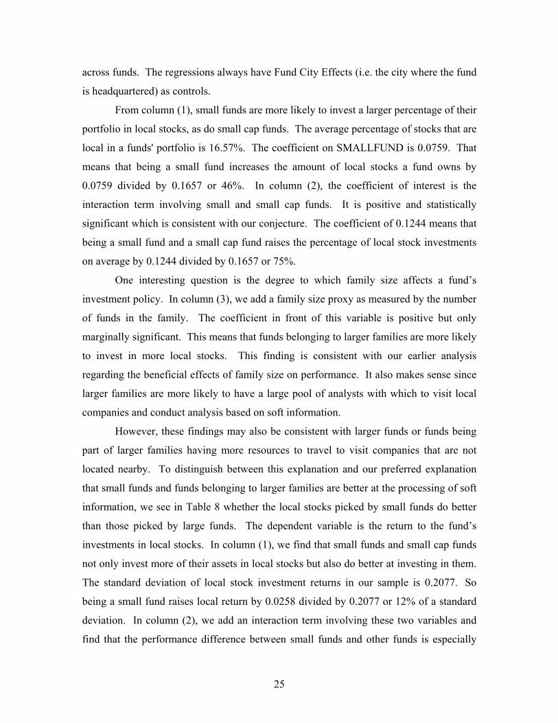
In Panels C and D, we split our benchmark sample in half to see whether our

estimates on LOGTNA and LOGFAMSIZE depend on particular sub-periods, 1963 to

1980 and 1981 to 1999. It appears that LOGTNA has a strong negative effect on

performance regardless of the sub-periods since the economic magnitudes are very

similar to those obtained in Table 3. We would not be surprised if the coefficients were

not statistically significant since we have smaller sample sizes in Panels C and D. But

17

even with only half the sample size, LOGTNA comes in significantly for a number of the

performance measures. In contrast, it appears that the effect of LOGFAMSIZE on

performance is much more pronounced in the latter half of the sample.

The analyses in Tables 3 and 4 strongly indicate that fund size is negatively

related to future fund performance. Moreover, we are able to rule out that this

relationship is driven by differences in fund styles or mechanical correlations of fund size

with other observable fund characteristics. However, there still remain a number of

potential explanations for this relationship.

Three potential explanations come to mind. First, the lagged fund size and

performance relationship is due to transactions costs associated with liquidity or price

impact. We call this the “liquidity hypothesis”. Second, perhaps investors in large funds

are less discriminating about returns than investors in small funds. One reason why this

might be the case is that large funds such as Magellan are better at marketing and are able

to attract investors through advertising. In contrast, small funds without such marketing

operations may need to rely more on better performance to attract and maintain investors.

We call this the “clientele hypothesis”. Third, fund size is inversely related to

performance because of fund incentives to lock in assets under management after a long

string of good past performances.11 When a fund is small and has little reputation, the

manager goes about the business of stock picking. But as the fund gets large because of

good past performance, the manager may for various reasons lock in his fund size by

being passive (or a “closet indexer” as practitioners put it). We call this the “agency-risk-

taking hypothesis”.

B. The Role of Liquidity: The Effect of Fund Size on Performance by Fund Styles

In order to narrow down the list of potential explanations, we design a test of the

liquidity hypothesis. To the extent that liquidity is driving our findings above, we would

11 More generally, it may be that after many years of good performance, bad performance follows for whatever reason. We are offering here a plausible economic mechanism for why this might come about. The ex ante plausibility of this alternative story is, however, somewhat mixed. On the one hand, the burgeoning empirical literature on career concerns suggests that fund managers ought to be bolder with past success (see, e.g., Chevalier and Ellison (1999) and Hong, Kubik and Solomon (2000)). On the other hand, the fee structure means that funds may want to lock in assets under management because investors are typically slow to pull their money out of funds (Brown, Harlow and Starks (1996), Chevalier and Ellison (1997)).

18

expect to see that fund size matters much more for performance among funds that have to

invest in small stocks (i.e. stocks with small market capitalization) than funds that get to

invest in large stocks. The reason is that small stocks are notoriously illiquid. As a

result, funds that have to invest in small stocks are more likely to need new stock ideas

with asset base growth, whereas large funds can simply increase their existing positions

without being hurt too much by price impact.

Importantly, this test of the liquidity hypothesis also allows us to discriminate

between the other two hypotheses. First, existing research finds that there is little

variation in incentives between “small cap” funds (i.e. funds that have to invest in small

stocks) and other funds (see, e.g., Almazan, et.al. (2001)). Hence, this prediction ought

to help us discriminate between our hypothesis and the alternative “agency-risk-taking”

story involving fund incentives. Moreover, since funds that have to invest in small stocks

tend to do better than other funds, it is not likely that our results are due to the clienteles

of these funds being more irrational than those investing in other funds. This allows us to

distinguish the liquidity story from the clientele story.

In the CRSP Mutual Fund Database, we are fortunate that each fund self-reports

its style, and so we look for style descriptions containing the words “small cap”. It turns

out that one style, “Small Cap Growth”, fits this criterion. It is likely that funds in this

category are likely to have to invest in small stocks by virtue of their style designation.

So, we identify funds in our sample as either Small Cap Growth if it has ever reported

itself as such or “Not Small Cap Growth”. (Funds rarely change their self-reported style.)

Unfortunately, funds with this designation are not prevalent until the early eighties.

Hence, through out the analysis in this section, we limit our sample to 1981 to 1999.

During this period, there are on average 165 such funds each year. The corresponding

number for the overall sample during this period is about 1000. So, Small Cap Growth

represents a small but healthy slice of the overall population. Also, the average TNA of

these funds is 212.9 million dollars with a standard deviation of 566.7 million dollars.

The average TNA of a fund in the overall sample is 431.5 million dollars with a standard

deviation of 1.58 billion dollars. So, Small Cap Growth funds are somewhat smaller than

the typical fund. But they are still quite big and there is a healthy fund size distribution

among them, so that we can measure the effect of fund size on performance. Indeed,

19

among funds below the top quintile of the fund size distribution, there is a negligible

difference in the size distributions of these two fund styles.

Table 5 reports what happens to the results in Table 3 when we augment the

regression specifications by including a dummy indicator Ind{not SCG} (that equals one if a

fund is not Small Cap Growth and zero otherwise) and an additional interaction term

involving LOGTNA and Ind{not SCG} as in Equation (5). We first report the results for

gross fund returns. The coefficient in front of LOGTNA is about –0.06 (across the four

performance benchmarks). Importantly, the coefficient in front of the interaction term is

positive and statistically significant (about 0.04 across the four performance

benchmarks). This is the sign predicted by the liquidity hypothesis since it says that for

Not Small Cap Growth funds, there is a smaller effect of fund size on performance. The

effect is economically interesting as well. Since the two coefficients, –0.06 and 0.04, are

similar in magnitude, this means that a sizeable fraction of the effect of fund size on

performance comes from small cap funds. The results using net fund returns reported in

Panel B are similar.

These findings suggest that liquidity plays a role in eroding performance.

Moreover, as many practitioners have pointed out, since managers of funds get

compensated on assets under management, they are not likely to voluntarily keep their

funds small just because it hurts the returns of their investors, who may not be aware of

the downside of scale (see Becker and Vaughn (2001) and Section V below for further

discussion).12

C. The Role of Organization: The Effect of Family Size on Performance

In this section, we delve a bit deeper into the liquidity hypothesis. As we pointed

out in the beginning of the paper, liquidity means that large funds need to find more stock

ideas than small funds, but it does not therefore follow that they cannot. Indeed, large

funds can go out and hire more managers to follow more stocks. To see that this is

possible, we calculate some basic summary statistics on fund holdings by fund size

quintiles. Since the CRSP Mutual Fund Database does not have this information, we turn

12 A related literature finds that mutual fund investors are susceptible to marketing (see, e.g., Gruber (1996), Sirri and Tufano (1998) and Zheng (1999)).

20

to the CDA Spectrum Database. We take data from the end of September 1997 and

calculate the number of stocks held by each fund. The median fund in the smallest fund

size quintile has about 16 stocks in its portfolio, while the median fund in the largest fund

size quintile has only about 66 stocks in its portfolio, even though the large funds are

many times bigger than their smaller counterparts. These numbers make clear that large

funds do have to find more stock ideas but that they do not significantly scale up the

number of stocks that they hold or cover relative to their smaller counterparts. At the

same time, they also make clear that there is plenty of scope for large funds to find other

stocks given the thousands of stocks available.

To see that assets under management need not be obviously bad for the

performance of a fund organization, recall from Table 3 that controlling for fund size,

assets under management of the other funds in the family that the fund belongs to

actually increases the fund’s performance. The coefficient in front of LOGFAMSIZE is

roughly 0.007 regardless of the performance benchmark used. One standard deviation of

this variable is 2.75, so a two standard deviation shock in the size of the family that the

fund belongs to leads to about a 3.85 basis points movement in the fund’s performance

next month (or about 46 basis points movement annual) depending on the performance

measure used. The effect is smaller than that of fund size on returns but is nonetheless

statistically and economically significant. In other words, assets under management are

not bad for a fund organization’s performance per se.

In Table 6, we extend our analysis of the effect of family size on fund returns by

seeing whether this effect varies across fund styles. Our hope is that family size is just as

important for Small Cap Growth funds as for other funds. After all, it is these funds that

are most affected by scale. For us to claim that scale is not bad per se, even accounting

for liquidity, we would like to find that the benefits of family size are derived by even

funds that are most affected by liquidity. To see whether this is the case, we augment the

regression specification in Table 5 by adding an interaction term involving

LOGFAMSIZE and the dummy indicator Ind{not SCG} (that equals one if a fund is not

Small Cap Growth and zero otherwise). The variable of interest is the coefficient in front

of this interaction term.

21

Panel A presents the regression results for funds in fund size quintiles two to five.

The coefficient in front of this interaction term is positive but is not statistically

significant. In other words, it does not appear that there are major differences between

the effect of family size on performance among Small Cap Growth funds and other funds.

This finding is as we had hoped for. To make sure that this finding holds more generally,

we re-estimate this regression specification using all funds. Now, the coefficient in front

of the interaction term is negative, but is again not statistically significant. Using either

sample, it does not appear that the effect of family size is limited to Not Small Cap

Growth funds. So we can be assured that funds do benefit from being part of a large

family.

These findings, fund performance declines with own fund size but increases with

the size of the other funds in the family, fit nicely with anecdotal evidence from industry

practitioners (see, e.g., Pozen (1998), Fredman and Wiles (1998)). According to these

anecdotes, in most families, major decisions are decentralized in that the fund managers

make stock picks without substantial coordination with other managers. So a family is an

organization that credibly commits to letting each of its fund managers run their own

assets. Moreover, being part of a family serves as a way to economize on fixed costs

associated with marketing or research. IvKovic (2002) argues that being part of a large

family may improve performance because of other spillovers.13 Whatever the exact

benefits of families may be, this finding makes clear that liquidity and scale need not be

bad for fund performance depending on how the fund is organized. After all, if a large

fund is organized like a fund family with a bunch of little funds ran by different

managers, then scale need not be bad per se, just as family size does not appear to be bad

for family performance.

D. Organizational Diseconomies and The Composition of Fund Investments

So, why then does it appear that scale erodes fund performance because of

liquidity? We hypothesize that in addition to liquidity, fund size erodes performance

because of organizational diseconomies. To make things concrete, imagine that there is a

13 In his analysis of family size, he happened to control for fund size and found that fund size indeed erodes performance. Though the goal of his paper was not to examine fund size, it is comforting to know that some of our baseline results have been independently verified.

22

small fund company X with one fund operated by one manager who picks the stocks.

Since the fund is small, the manager can easily invest the assets under management by

generating a few stock ideas. Now imagine that there is a large fund Y in which the

manager no longer has the capacity to invest all the money. So the manager needs other

co-managers to help him run the fund. For fund Y, the stock picks need to be

coordinated among many more agents and therefore organizational form (e.g. flat versus

hierarchical forms) becomes important. As such, organizational diseconomies may arise.

There are many types of organizational diseconomies that lead to different

predictions on why small organizations outperform large ones. One set of diseconomies,

from the work of Williamson (1975, 1988), includes bureaucracy and related

coordination costs. Another set of diseconomies comes from the influence-cost literature

(see, e.g., Milgrom and Roberts (1988)). Yet another set of diseconomies centers on the

adverse effects of hierarchies (or authority) for the incentives of agents who do not have

any control over asset-allocation decisions (see, e.g., Aghion and Tirole (1997), Stein

(2002)).

Interestingly, the findings in Tables 3 and 6 already allow us to discriminate

among different types of organizational diseconomies. For instance, if Williamsonian

diseconomies are behind the relationship between size and performance, then one expects

that funds that belong to large families do worse, since bureaucracy ought to be more

important in huge fund complexes. The fact that we find the opposite indicates that

bureaucracy is not likely an important reason behind why performance declines with fund

size.

We conjecture that hierarchy costs may be especially relevant for mutual funds

since many funds, even very large ones, are typically directed by a single manager who is

at the top of a hierarchy managing junior managers or analysts. The basic idea is that if

the manager at the top of the hierarchy undercuts the decisions of those at the bottom,

then those below him may not invest time in certain types of research. As a result, efforts

to uncover certain investment ideas in this setting are diminished relative to a situation in

which the junior managers or analysts controlled their own smaller funds. So all else

equal, large funds may perform worse than small ones.

23

We take a closer look at the effect of organizational diseconomies due to

hierarchy costs on fund performance by testing some predictions from Stein (2002).

Stein (2002) argues that in the presence of such hierarchy costs, small organizations

ought to outperform large ones at tasks that involve the processing of soft information,

(i.e., information that cannot be directly verified by anyone other than the agent who

produces it). If the information is soft, then agents have a hard time convincing their

superiors of their ideas. Stein’s analysis also indicates that large organizations may

actually be very efficient at processing hard information. In the context of the mutual

fund industry, one can think of passive funds that mimic indices as primarily processing

hard information. As such, one would expect these types of funds to not be very much

affected by scale. Two pieces of evidence are consistent with this prediction. First,

Vanguard seems to dominate the business for index funds. Indeed, for indexers, being

large is an asset since one can then acquire better tracking technologies and better

computer programmers. Second, our evidence in Table 5, that fund size only affects

small cap funds, is consistent with this observation since most index funds, which tend to

mimic the S&P 500 index, trade predominantly large stocks.

To the extent that fund size erodes performance because of the type of

organizational diseconomies pointed out by Stein (2002), we expect that small funds are

better than large ones at the processing of soft information. To test this prediction, we

compare the investments of large and small funds in local stocks (companies located near

where a fund is headquartered). Investing in such companies requires that the

organization process soft information as opposed to a strictly quantitative investing

approach, which would typically process hard information like price-to-earnings ratios.

Our work in testing this prediction builds on the very interesting work of Coval and

Moskowitz (2001) whose central thesis is that mutual fund managers do have ability

when it comes to local stocks. Anecdotal evidence indicates that this ability comes in the

form of processing soft information like talking and evaluating CEOs of local companies.

They find that funds can earn superior returns on their local investments. We focus on

the effect of size on investment among small cap funds. We are also interested in the

effect of family size on the composition of fund investments.

24

The CDA Spectrum Database does not have the same information on fund

characteristics as the CRSP Mutual Fund Database. Luckily, we are able to construct

from the fund stock holdings data a proxy for fund size, which is simply the value of the

fund’s stock portfolio at the end of a quarter. While this is not exactly the same as the

asset base since funds hold cash and bonds, we believe that the proxy is a reasonable one

since we can look at the tails of the size distribution to draw inferences, i.e. compare very

small funds to other funds. Moreover, the noise in our fund size measure does not

obviously bias our estimates.

In addition, we can construct better style controls for each fund by looking at their

stock holdings. We use a style measure constructed by Daniel, Grinblatt, Titman and

Wermers (1997), which we call the DGTW style adjustments. For each month, each

stock in our sample is characterized by where they fall in the (across stocks) size

quintiles, book-to-market quintiles and price momentum quintiles. So a stock in the

bottom of the size, book-to-market and momentum quintiles in a particular month would

be characterized by a triplet (1,1,1). For each fund, we can characterize its style along the

size, book-to-market and momentum dimension by taking the average of the DGTW

characteristics of the stocks in their portfolio weighted by the percentage of the value of

their portfolio that they devote to each stock. We can then define a small cap fund as one

whose DGTW size measure falls in the bottom 10 percent when compared to other funds.

Table 7 reports the effect of fund size on the percentage of the value of a fund’s

portfolio devoted to local stocks, where locality is defined relative to the headquarter of

the fund as in Coval and Moskowitz (2001). More specifically, a stock is considered a

local fund investment if the headquarter of the company is in the same Census region as

the mutual fund’s headquarter.14 The dependent variable is the value of the local stocks

in the fund portfolio divided by the total value of the stocks in the fund portfolio. The

first independent variable is SMALLFUND, which is a dummy variable that equals one if

the fund is in the bottom 10% of the fund size distribution. SMALLCAPFUND equals

one if a fund has an average DGTW size score for its stocks that is in the bottom 10% 14 There are nine Census regions: New England (CT, ME, NH, RI, VT); Middle Atlantic (NJ, NY, PA); East North Central (IL, IN, MI, OH, WI); West North Central (IA, KS, MN, MO, NE, ND, SD); South Atlantic (DE, FL, GA, MD, NC, SC, VA, WV); East South Central (AL, KY, MS, TN); West South Central (AR, LA, OK, TX); Mountain (AZ, CO, ID, MT, NE, NM, UT, WY); and Pacific (AK, CA, HI, OR, WA).

25

across funds. The regressions always have Fund City Effects (i.e. the city where the fund

is headquartered) as controls.

From column (1), small funds are more likely to invest a larger percentage of their

portfolio in local stocks, as do small cap funds. The average percentage of stocks that are

local in a funds' portfolio is 16.57%. The coefficient on SMALLFUND is 0.0759. That

means that being a small fund increases the amount of local stocks a fund owns by

0.0759 divided by 0.1657 or 46%. In column (2), the coefficient of interest is the

interaction term involving small and small cap funds. It is positive and statistically

significant which is consistent with our conjecture. The coefficient of 0.1244 means that

being a small fund and a small cap fund raises the percentage of local stock investments

on average by 0.1244 divided by 0.1657 or 75%.

One interesting question is the degree to which family size affects a fund’s

investment policy. In column (3), we add a family size proxy as measured by the number

of funds in the family. The coefficient in front of this variable is positive but only

marginally significant. This means that funds belonging to larger families are more likely

to invest in more local stocks. This finding is consistent with our earlier analysis

regarding the beneficial effects of family size on performance. It also makes sense since

larger families are more likely to have a large pool of analysts with which to visit local

companies and conduct analysis based on soft information.

However, these findings may also be consistent with larger funds or funds being

part of larger families having more resources to travel to visit companies that are not

located nearby. To distinguish between this explanation and our preferred explanation

that small funds and funds belonging to larger families are better at the processing of soft

information, we see in Table 8 whether the local stocks picked by small funds do better

than those picked by large funds. The dependent variable is the return to the fund’s

investments in local stocks. In column (1), we find that small funds and small cap funds

not only invest more of their assets in local stocks but also do better at investing in them.

The standard deviation of local stock investment returns in our sample is 0.2077. So

being a small fund raises local return by 0.0258 divided by 0.2077 or 12% of a standard

deviation. In column (2), we add an interaction term involving these two variables and

find that the performance difference between small funds and other funds is especially

26

big in small cap funds. In column (3), we add in a family size proxy as measured by the

number of funds in the family. Similar results obtain using total net assets for the family.

This does not do much to our variables of interest though it is positive but only

marginally significant. So it appears that a fund that belongs to a large family does better

in their local stock investments.

The findings in Table 8 suggest that the performance differences between small

and large funds have something to do with their different ability to invest in local stocks.

Note that Tables 7 and 8 only report the results using the cross-section in September

1997. We have replicated our analysis using the other quarters in the period of 1997 to

1998. The results are very robust across quarters.

Our analysis here is similar to the work of Berger, Miller, Petersen, Rajan and

Stein (2002). They test the idea in Stein (2002) that small organizations are better than

large ones in activities that require the processing of soft information in the context of

bank lending to small firms. They find that large banks are less willing than small ones

to lend to informationally difficult credits such as firms that do not keep formal financial

records. They also find that large banks lend at a greater distance, interact more

impersonally with their borrowers, have shorter and less exclusive relationships and do

not alleviate credit constraints as effectively. Interestingly, they find that the size of the

bank-holding company that a bank belongs to does not affect the lending policies of the

bank. In other words, size itself is not necessarily bad for banks. This finding is

analogous to our finding regarding the neutral to beneficial effects of family size on fund

performance.

V. Alternative Explanations and Further Discussions

In Section IV, we have already ruled out a number of alternative explanations for

our findings in establishing the role of liquidity and organization in mediating the

relationship between fund size and performance. In this section, we discuss additional

alternative explanations. One institutional reason for our finding may be that it is easier

for fund families to manipulate the performance of small funds in small cap stocks.

While this alternative explanation is possible, we do not think that it is driving our results

for several reasons. First, we exclude the very smallest funds for which this is likely and

27

our results are unchanged. Moreover, in analysis that is not reported for reasons of

brevity, we have also dropped out very young funds, for which such manipulation is most

likely and our results are again unchanged. Finally, such manipulation cannot account

for the relationship between fund size and the composition of fund investments

documented in Section IV.D.

Besides such institutional reasons, it may be the case that our findings are due to

other organizational-related issues as well the hierarchy cost hypothesis presented in

Section IV.D. For instance, many managers often talk about how difficult it is train new

hires when their fund gets big and they need to find help. We view such comments as

broadly supportive of our contention that organization matters for fund performance.

However, we readily admit that we do not currently have the data to completely rule out

every alternative interpretation.

Ideally, we would like to have information about the incentives inside fund

organizations. For instance, our hierarchy cost hypothesis also suggests that a crucial

unobservable determinant of fund performance is the nature of the incentives inside the

fund.15 More concretely, suppose that the organizational diseconomies are due to the

adverse effects of a hierarchy on managerial effort. Then an optimal organizational

structure is to limit managers to a small pot of money and let them manage it as they

choose. With such an organizational structure, scale may not affect performance. This is

exactly what happens at the family level and probably why performance does not decline

with family size. Indeed, some fund families such as the Capital Group do adopt such an

organizational structure. However, it is not so easy for every fund family to adopt such

an organizational form since managers will need to be compensated in other ways if their

fund size is capped.16

15 With this in mind, an interesting question is whether our hypothesis predicts that the ratio of fund size to number of people in the organization ought to be a determinant of fund performance, i.e. the higher this ratio, is the worst the performance? The answer is no since it depends on how the fund is organized. A fund with a very low ratio of fund size to number of people may do worse without the right organizational form. Interestingly, Prather and Middleton (2002) find that the number of people managing a fund does not seem to predict performance. 16 Indeed, the Capital Group follows a partnership track in which successful managers are given an ownership stake in the mutual fund organization. We thank Jack MacDonald for pointing this example out to us.

28

VI. Conclusion

To the best of our knowledge, we are the first to find strong evidence that fund

size erodes performance. We then move on to consider various explanations for why this

might be the case. We find that this relationship is not driven by heterogeneity in fund

styles, fund size being correlated with other observable fund characteristics, or any type

of survivorship bias. Instead, we find that the effect of fund size on fund returns is most

pronounced for funds that play small cap stocks. This suggests that liquidity is an

important reason behind why size erodes performance. Moreover, we argue that

organizational diseconomies related to hierarchy costs may also play a role in addition to

liquidity in the documented diseconomies of scale. Consistent with this view, we find

that funds that belong to large families do better than other funds and that small funds do

better in their investments in local stocks than large funds.

Importantly, our findings have relevance for the ongoing research into the

question of Coase (1937) regarding the determinants of the boundaries of the firm. While

an enormous amount of theoretical research has been done on this question, there has

been far less empirical work. Our findings suggest that mutual funds may be an

invaluable laboratory with which to study related issues in organization. Unlike most

corporations, data on mutual funds are plentiful because of disclosure regulations and the

tasks and performance of mutual funds are measurable. We plan to better refine our

understanding of the nature of organizations in the future using this laboratory.

29

References

Aghion, Philippe and Jean Tirole, 1997, Formal and real authority in organizations, Journal of Political Economy 105, 1-29.

Almazan, Andres, Keith C. Brown, Murray Carlson and David A. Chapman,

2001, Why constrain your mutual fund manager?, University of Texas Working Paper.

Becker, Stan and Greg Vaughan, 2001, Small is beautiful, Journal of Portfolio Management (Summer), 9-17.

Berger, Allen N., Nathan H. Miller, Mitchell A. Petersen, Raghuram G. Rajan, and Jeremy C. Stein, 2002, Does function follow organizational form? Evidence from the lending practices of large and small banks, Harvard University Working Paper.

Berk, Jonathan and Richard C. Green, 2002, Mutual fund flows and performance

in rational markets, U.C. Berkeley Working Paper. Bolton, Patrick, and David S. Scharfstein, 1998, Corporate finance, the theory of

the firm, and organizations, Journal of Economic Perspectives 12, 95-114. Brown, Keith, V.W. Harlow and Laura Starks, 1996, Of tournaments and temptations: An analysis of managerial incentives in the mutual fund industry, Journal of Finance 51, 85-110.

Carhart, Mark M., 1997, On persistence in mutual fund performance, Journal of Finance, Vol. LII, 57-82. Carhart, Mark M., Jennifer Carpenter, Anthony Lynch and David Musto, 2002, Mutual fund survivorship, Review of Financial Studies 15, forthcoming.

Chen, Joseph, Harrison Hong and Jeremy C. Stein, 2002, Breadth of ownership and stock returns, Journal of Financial Economics, forthcoming.

Chevalier, Judith A., and Glenn D. Ellison, 1997, Risk taking by mutual funds as

a response to incentives, Journal of Political Economy 105, 1167-1200.

Chevalier, Judith A., and Glenn D. Ellison, 1999, Career concerns of mutual fund managers, Quarterly Journal of Economics 114, 389-432.

Coase, Ronald H., 1937, The nature of the firm, Economica 4, 386-405.

Coval, Joshua D. and Tobias J. Moskowitz, 2001, The geography of investment:

Informed trading and asset prices, Journal of Political Economy 4, 811-841.

30

Daniel, Kent, Mark Grinblatt, Sheridan Titman and Russ Wermers, 1997, Measuring mutual fund performance with characteristic-based benchmarks, Journal of Finance, 52, 1035-1058. Elton, Edwin J., Martin J. Gruber and Christopher R. Blake, 2001, A first look at the accuracy of the CRSP Mutual Fund Database and a comparison of the CRSP and Morningstar Mutual Fund Databases, Journal of Finance, Vol. LVI, 2415-2430. Falkenstein, Eric G., 1996, Preferences for stock characteristics as revealed by mutual fund portfolio holdings, Journal of Finance, 51, 111-135.

Fama, Eugene F. and French, Kenneth R., 1993, “Common Risk Factors in the Returns on Stocks and Bonds,” Journal of Financial Economics 33, 3-56.

Fama, Eugene F. and MacBeth, James D., 1973, “Risk, Return and Equilibrium: Empirical Tests,” Journal of Political Economy 81, 607-636.

Fredman, Albert J. and Russ Wiles, 1998, How Mutual Funds Work, (Prentice

Hall, New Jersey). Gompers, Paul and Andrew Metrick, 2001, “Institutional investors and equity

prices,” Quarterly Journal of Economics 116, 229-259.

Grinblatt, Mark and Sheridan Titman, 1989, Mutual fund performance: An analysis of quarterly portfolio holdings, Journal of Business 62, 393-416.

Grinblatt, Mark, Sheridan Titman and Russ Wermers, 1995, Momentum

investment strategies, portfolio performance and herding: A study of mutual fund behavior, American Economic Review, 85, 1088-1105.

Grossman, Sanford J. and Oliver D. Hart, 1986, The costs and benefits of

ownership: A theory of vertical and lateral integration, Journal of Political Economy 94, 691-719.

Gruber, Martin J., 1996, Another puzzle: The growth in actively managed mutual funds, Journal of Finance, Vol. LI, 783-810.

Hart, Oliver D., 1995, Firms, Contracts and Financial Structure (Oxford

University Press, Oxford). Hart, Oliver D. and John Moore, 1990, Property rights and the nature of the firm,

Journal of Political Economy 98, 1119-1158. Holmstrom, Bengt and John Roberts, 1998, The boundaries of the firm revisited,

Journal of Economic Perspectives 12, 73-94.

31

Hong, Harrison, Jeffrey D. Kubik, and Amit Solomon, 2000, Security analysts’ career concerns and the herding of earnings forecasts, RAND Journal of Economics 31, 121-144.

Hong, Harrison, Terence Lim and Jeremy C. Stein, 2000, Bad news travels slowly: Size, analyst coverage, and the profitability of momentum strategies, Journal of Finance, Vol. LV, 265-295.

Investment Company Institute, 2000, Mutual Fund Fact Book, (Investment

Company Institute: Washington DC). IvKovic, Zoran, 2002, Spillovers in mutual fund families: Is blood thicker than

water? University of Illinois Working Paper.

Jegadeesh, Narasimhan and Titman, Sheridan, 1993, “Returns to Buying Winners and Selling Losers: Implications for Stock Market Efficiency,” Journal of Finance 48, 93-130. Jensen, Michael C., 1968, The performance of mutual funds in the period 1945-1964, Journal of Finance, 50, 549-572.

Lowenstein, Roger, 1997, Frightened funds: Is there a master in the house?, Wall Street Journal.

Malkiel, Burton G., 1995, returns from investing in equity mutual funds, 1971-

1991, Journal of Finance, 50, 549-572.

Milgrom, Paul R. and John Roberts, 1988, An economic approach to influence activities in organizations, American Journal of Sociology 94 Supplement, 154-179.

Newey, Whitney K. and Kenneth D. West, 1987, A simple positive-definite

heteroskedasticity and autocorrelation consistent covariance matrix, Econometrica 55, 703-708.

Perold, Andre and Robert S. Salomon, 1991, The right amount of assets under management, Financial Analysts Journal, 47, 31-39.

Pozen, Robert C., 1998, The Mutual Fund Business, (Cambridge, Mass: MIT

Press). Prather, Larry J. and Karen L. Middleton, 2002, Are N+1 heads better than one?

The case of mutual fund managers, Journal of Economic Behavior and Organization, 47, 103-120.

Sharpe, William F., 1964, Capital asset prices: A theory of market equilibrium under conditions of risk, Journal of Finance 19, 425-42.

32

Sirri, Eric R and Peter Tufano, 1998, Costly search and mutual fund inflows,

Journal of Finance 53, 1589-1622.

Stein, Jeremy C., 2002, Information production and capital allocation: Decentralized vs. hierarchical firms, Journal of Finance, forthcoming.

Wermers, Russ, 2000, Mutual fund performance: An empirical decomposition into stock-picking talent, style, transactions costs and expenses, Journal of Finance, Vol. LV, 1655-1695.

Williamson, Oliver E., 1975, Markets and Hierarchies: Analysis and Antitrust Implications, (Collier MacMillan, New York).

Williamson, Oliver E., 1988, Corporate finance and corporate governance,

Journal of Finance, 43, 567-591. Zheng, Lu, 1999, Is money smart? A study of mutual fund investors’ fund

selection ability, Journal of Finance, Vol. LIV, 901-933.

33

Table 1: Summary Statistics This table reports summary statistics for the funds in our sample. The Number of Funds is the number of mutual funds that meet our selection criteria for being an active mutual fund in each month. TNA is the total net assets under management in millions of dollars. LOGTNA is the logarithm of TNA. LOGFAMSIZE is the logarithm of one plus the assets under management of the other funds in the family that the fund belongs to (excluding the asset base of the fund itself). TURNOVER is fund turnover, defined as the minimum of aggregate purchases and sales of securities divided by the average TNA over the calendar year. AGE is the number of years since the organization of the fund. EXPRATIO is the total annual management fees and expenses divided by year-end TNA. TOTLOAD is the total front-end, deferred and rear-end charges as a percentage of new investments. FLOW is the percentage new fund flow into the mutual fund over the past year. TNA, LOGFAMSIZE and FLOW are reported monthly. All other fund characteristics are reported once a year. FUNDRET is the monthly market-adjusted fund return. These returns are calculated before (gross) and after (net) deducting fees and expenses. Panel A reports the time-series averages of monthly cross-sectional averages and monthly cross-sectional standard deviations (shown in brackets) of fund characteristics. Panels B and C report the time-series averages of the cross-sectional correlations between fund characteristics. Panel D reports the time-series averages of monthly cross-sectional averages of market-adjusted fund returns. In Panels A and B, fund size quintile 1 (5) has the smallest (largest) funds. The sample is from January 1963 to December 1999. Panel A: Time-series averages of cross-sectional averages and standard deviations.

Mutual Fund Size Quintile 1 2 3 4 5 All Funds

Quintiles 2-5

Number of Funds 148.2 147.8 147.8 147.8 147.3 741.4 590.6

4.7 22.2 60.6 165.4 1164.7 282.5 352.3 TNA ($ million) [3.2] [7.2] [16.6] [54.8] [1797.1] [925.8] [1022.7]

1.09 2.94 3.96 4.94 6.45 3.87 4.57 LOGTNA ($ million) [1.01] [0.34] [0.27] [0.33] [0.75] [1.92] [1.38]

3.70 4.52 5.29 5.91 7.00 5.28 5.68 LOGFAMSIZE ($ million) [2.98] [2.89] [2.72] [2.56] [2.16] [2.92] [2.75]

42.07 55.68 59.09 61.20 52.17 54.17 57.07 TURNOVER (% per year) [83.03] [74.00] [68.60] [64.28] [54.56] [71.84] [67.21]

8.17 11.90 14.82 18.43 25.16 15.67 17.57 AGE (years) [8.54] [10.73] [12.85] [14.38] [15.06] [13.96] [14.33]

1.29 1.08 0.94 0.85 0.68 0.97 0.89 EXPRATIO (% per year) [1.11] [0.59] [0.46] [0.37] [0.31] [0.68] [0.48]

3.41 4.19 4.32 4.57 5.28 4.36 4.59 TOTLOAD (%) [3.32] [3.32] [3.34] [3.39] [2.88] [3.36] [3.32]

30.79 30.66 26.97 21.27 13.54 24.67 23.13 FLOW (% per year) [113.55] [113.36] [101.66] [84.08] [59.04] [102.64] [96.60]

34

Panel B: Time-series averages of (monthly) correlations between fund characteristics. [Using all funds]

TNA

LOG- TNA

LOG- FAMSIZE

TURN- OVER

AGE

EXP- RATIO

TOT- LOAD

FLOW

TNA 1.00 0.56 0.24 -0.05 0.27 -0.19 0.10 -0.03LOGTNA 1.00 0.40 0.06 0.44 -0.31 0.19 -0.07LOGFAMSIZE 1.00 0.08 0.08 -0.19 0.25 -0.01TURNOVER 1.00 0.01 0.17 0.05 -0.01AGE 1.00 -0.13 0.19 -0.18EXPRATIO 1.00 -0.05 0.08TOTLOAD 1.00 -0.04FLOW 1.00 Panel C: Time-series averages of (monthly) correlations between fund characteristics. [Excluding smallest 20% of funds]

TNA

LOG- TNA

LOG- FAMSIZE

TURN- OVER

AGE

EXP- RATIO

TOT- LOAD

FLOW

TNA 1.00 0.66 0.23 -0.08 0.24 -0.24 0.09 -0.03LOGTNA 1.00 0.35 -0.05 0.37 -0.36 0.13 -0.07LOGFAMSIZE 1.00 0.07 0.03 -0.17 0.22 -0.01TURNOVER 1.00 -0.04 0.26 0.03 0.01AGE 1.00 -0.18 0.17 -0.19EXPRATIO 1.00 0.01 0.10TOTLOAD 1.00 -0.05FLOW 1.00 Panel D: Time-series averages of (monthly) cross –sectional averages of market-adjusted fund returns.

Mutual Fund Size Quintile 1 2 3 4 5 All Funds

Quintiles 2-5

0.09% 0.02% 0.03% -0.06% -0.06% 0.01% -0.02% FUNDRET (Gross) [3.04%] [2.64%] [2.61%] [2.46%] [2.00%] [2.62%] [2.48%]

-0.02% -0.07% -0.05% -0.13% -0.12% -0.08% -0.09% FUNDRET (Net) [3.04%] [2.64%] [2.61%] [2.46%] [2.00%] [2.62%] [2.48%]

35

Table 2: Summary Statistics for Performance Benchmarks This table reports the loadings of the five (equal-weighted) TNA-sorted fund portfolios on various factors. Panel A reports the summary statistics for the factors. VWRF is the return on the CRSP value-weighted stock index in excess of the one-month Treasury rate. SMB is the return on a portfolio of small stocks minus large stocks. HML is the return on a portfolio long high book-to-market stocks and short low book-to-market stocks. MOM12 is the return on a portfolio long stocks that are past twelve-month winners and short those that are past twelve-month losers. Panel B reports the loadings calculated using the CAPM. Panel C reports the loadings calculated using the Fama-French (1993) 3-Factor model and this model augmented with the momentum factor (4-Factor model). The sample period is from January 1963 to December 1999. Panel A: Summary statistics of the factors.

Cross-correlations Factor Mean return

SD of return VWRF SMB HML MOM12

VWRF 0.58% 4.37% 1.00 0.32 -0.39 -0.02 SMB 0.17% 2.90% 1.00 -0.16 -0.30 HML 0.34% 2.63% 1.00 -0.15 MOM12 0.96% 3.88% 1.00 Panel B: Loadings calculated using the CAPM

CAPM Portfolio Alpha VWRF

1 (small) 0.04% 0.872 -0.02% 0.913 -0.01% 0.934 -0.09% 0.925 (large) -0.07% 0.91

Panel C: Loadings calculated using the 3-Factor model and the 4-Factor model

3-Factor model 4-Factor model Portfolio Alpha VWRF SMB HML Alpha VWRF SMB HML MOM12

1 (small) 0.01% 0.82 0.29 0.03 -0.02% 0.82 0.30 0.04 0.032 -0.03% 0.84 0.27 -0.01 -0.09% 0.85 0.30 0.00 0.053 0.01% 0.87 0.22 -0.05 -0.06% 0.87 0.25 -0.03 0.064 -0.06% 0.87 0.18 -0.05 -0.13% 0.87 0.20 -0.04 0.065 (large) -0.05% 0.88 0.08 -0.06 -0.10% 0.88 0.10 -0.05 0.05

36

Table 3: Regression of Fund Performance on Lagged Fund Size This table shows the Fama-Macbeth (1973) estimates of monthly fund returns regressed on fund characteristics lagged one month. The sample includes only funds that fall within fund size quintiles two to five. Fund returns are calculated before (gross) and after (net) deducting fees and expenses. These returns are adjusted using the market model, the CAPM, the Fama-French (1993) 3-Factor model, and the 4-Factor model. The dependent variable is FUNDRET. LOGTNA is the natural logarithm of TNA. LOGFAMSIZE is the natural logarithm of one plus the size of the family that the fund belongs to. TURNOVER is fund turnover and AGE is the number of years since the organization of the mutual fund. EXPRATIO is the total annual management fees and expenses divided by TNA. TOTLOAD is the total front-end, deferred and rear-end charges as a percentage of new investments. FLOW is the percentage new fund flow into the mutual fund over the past one year. LAGFUNDRET is the cumulative (buy-hold) fund return over the past twelve months. The sample is from January 1963 to December 1999. The t-statistics are adjusted for serial correlation using Newey-West (1987) lags of order three and are shown in parentheses.

Gross fund returns Net fund returns Market-Adj Beta-Adj 3-Factor 4-Factor Market-Adj Beta-Adj 3-Factor 4-Factor

0.056 0.087 0.080 0.019 0.026 0.056 0.049 -0.011 INTERCEPT (0.96) (1.63) (1.28) (0.30) (0.44) (1.05) (0.79) (0.18) -0.028 -0.028 -0.023 -0.020 -0.025 -0.025 -0.020 -0.018 LOGTNAi,t-1 (3.02) (3.04) (2.42) (2.15) (2.75) (2.76) (2.16) (1.89) 0.007 0.007 0.007 0.007 0.007 0.007 0.007 0.007 LOGFAMSIZEi,t-1 (2.26) (2.27) (2.22) (2.21) (2.33) (2.34) (2.29) (2.28) 0.000 0.000 0.000 0.000 0.000 0.000 0.000 0.000 TURNOVERi,t-1 (0.85) (0.86) (0.85) (0.83) (0.77) (0.78) (0.77) (0.75) -0.001 -0.001 -0.001 -0.001 0.000 0.000 -0.001 -0.001 AGEi,t-1 (0.62) (0.62) (0.64) (0.63) (0.52) (0.53) (0.55) (0.54) -0.004 -0.004 -0.007 -0.007 -0.039 -0.038 -0.041 -0.041 EXPRATIOi,t-1 (0.11) (0.09) (0.18) (0.18) (0.97) (0.95) (1.04) (1.05) 0.003 0.003 0.003 0.003 0.003 0.003 0.003 0.003 TOTALLOADi,t-1 (1.26) (1.25) (1.26) (1.29) (1.21) (1.20) (1.21) (1.25) 0.000 0.000 0.000 0.000 0.000 0.000 0.000 0.000 FLOWi,t-1 (0.50) (0.50) (0.51) (0.49) (0.47) (0.47) (0.48) (0.46) 0.029 0.028 0.028 0.029 0.029 0.029 0.029 0.029 LAGFUNDRETi,t-1 (6.00) (5.98) (6.00) (5.99) (6.03) (6.01) (6.03) (6.02)

No. of months 444 444 444 444 444 444 444 444

37

Table 4: Regression of Fund Returns on Lagged Fund Size, Robustness Checks This table presents robustness checks of the regression specification in Table 3. In Panel A, the sample includes all funds. In Panel B, the dependent variable is twelve-month fund returns and the regressions are non-overlapping. In Panel C, the sample consists of only observations from 1963 to 1980. In Panel D, the sample consists of only observations from 1981 to 1999. LOGTNA is the natural logarithm of TNA. LOGFAMSIZE is the natural logarithm of one plus the size of the family that the fund belongs to. Estimates of the intercept and other independent variables are omitted for brevity. The other independent variables include TURNOVER, AGE, EXPRATIO, TOTLOAD, FLOW, and LAGFUNDRET. The t-statistics are adjusted for serial correlation using Newey-West (1987) lags of order three and are shown in parentheses. Panel A: Sample includes all funds

Gross fund returns Net fund returns Market-Adj Beta-Adj 3-Factor 4-Factor Market-Adj Beta-Adj 3-Factor 4-Factor

-0.023 -0.026 -0.019 -0.021 -0.020 -0.022 -0.015 -0.017 LOGTNAi,t-1 (2.59) (2.94) (2.22) (2.48) (2.16) (2.49) (1.76) (2.02) 0.006 0.006 0.006 0.006 0.006 0.006 0.006 0.006 LOGFAMSIZEi,t-1 (1.99) (2.03) (1.99) (2.05) (2.10) (2.15) (2.11) (2.17)

No. of months 444 444 444 444 444 444 444 444 Panel B: Dependent variable is twelve-month (non-overlapping) fund returns

Gross fund returns Net fund returns Market-Adj Beta-Adj 3-Factor 4-Factor Market-Adj Beta-Adj 3-Factor 4-Factor

-0.436 -0.440 -0.345 -0.312 -0.402 -0.406 -0.312 -0.280 LOGTNAi,t-1 (3.26) (3.27) (2.40) (2.19) (3.07) (3.07) (2.20) (1.99) 0.088 0.089 0.088 0.088 0.090 0.091 0.090 0.090 LOGFAMSIZEi,t-1 (2.05) (2.06) (2.05) (2.07) (2.10) (2.12) (2.11) (2.12)

No. of years 37 37 37 37 37 37 37 37

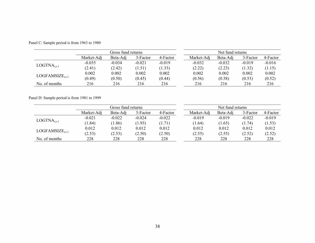
38

Panel C: Sample period is from 1963 to 1980

Gross fund returns Net fund returns Market-Adj Beta-Adj 3-Factor 4-Factor Market-Adj Beta-Adj 3-Factor 4-Factor

-0.035 -0.034 -0.021 -0.019 -0.032 -0.032 -0.019 -0.016 LOGTNAi,t-1 (2.41) (2.42) (1.51) (1.33) (2.22) (2.23) (1.32) (1.15) 0.002 0.002 0.002 0.002 0.002 0.002 0.002 0.002 LOGFAMSIZEi,t-1 (0.49) (0.50) (0.45) (0.44) (0.56) (0.58) (0.53) (0.52)

No. of months 216 216 216 216 216 216 216 216 Panel D: Sample period is from 1981 to 1999

Gross fund returns Net fund returns Market-Adj Beta-Adj 3-Factor 4-Factor Market-Adj Beta-Adj 3-Factor 4-Factor

-0.021 -0.022 -0.024 -0.022 -0.019 -0.019 -0.022 -0.019 LOGTNAi,t-1 (1.84) (1.86) (1.93) (1.71) (1.64) (1.65) (1.74) (1.53) 0.012 0.012 0.012 0.012 0.012 0.012 0.012 0.012 LOGFAMSIZEi,t-1 (2.53) (2.53) (2.50) (2.50) (2.55) (2.55) (2.52) (2.52)

No. of months 228 228 228 228 228 228 228 228

39

Table 5: Effect of Fund Size on Performance by Fund Style This table reports the Fama-Macbeth (1973) estimates of monthly fund returns regressed on fund characteristics lagged one month. The sample includes only funds that fall within fund size quintiles two to five. Fund returns are calculated before (gross) and after (net) deducting fees and expenses. These fund returns are adjusted using the market model, the CAPM, the Fama-French (1993) 3-Factor model, and the 4-Factor model. The regression specification is the one in Table 3 but augmented with Ind{not SCG}, which is a dummy variable that equals one if the self-reported fund style is not Small Cap Growth and zero otherwise and this indicator variable interacted with LOGTNA. The sample is from January 1981 to December 1999. The t-statistics are adjusted for serial correlation using Newey-West (1987) lags of order three and are shown in parentheses.

Gross fund returns Net fund returns Market-Adj Beta-Adj 3-Factor 4-Factor Market-Adj Beta-Adj 3-Factor 4-Factor

0.205 0.257 0.320 0.263 0.175 0.226 0.289 0.231 INTERCEPT (1.27) (1.53) (2.44) (1.98) (1.08) (1.34) (2.20) (1.75) -0.250 -0.252 -0.260 -0.262 -0.249 -0.251 -0.259 -0.261 IND{not SCG} (1.54) (1.55) (1.62) (1.63) (1.53) (1.54) (1.61) (1.62) -0.058 -0.058 -0.063 -0.061 -0.055 -0.056 -0.060 -0.058 LOGTNAi,t-1 (3.15) (3.17) (3.40) (3.29) (3.03) (3.05) (3.28) (3.17) 0.040 0.041 0.043 0.044 0.040 0.041 0.043 0.044 LOGTNAi,t-1 *

IND{not SCG} (2.36) (2.39) (2.53) (2.56) (2.35) (2.37) (2.52) (2.55) 0.012 0.012 0.011 0.011 0.012 0.012 0.012 0.012 LOGFAMSIZEi,t-1 (2.57) (2.57) (2.54) (2.54) (2.59) (2.59) (2.57) (2.56) 0.000 0.000 0.000 0.000 0.000 0.000 0.000 0.000 TURNOVERi,t-1 (1.62) (1.61) (1.62) (1.61) (1.57) (1.56) (1.57) (1.57) -0.001 -0.001 -0.001 -0.001 -0.001 -0.001 -0.001 -0.001 AGEi,t-1 (0.98) (0.97) (0.98) (0.97) (0.87) (0.87) (0.88) (0.87) -0.018 -0.018 -0.019 -0.019 -0.062 -0.062 -0.064 -0.063 EXPRATIOi,t-1 (0.44) (0.43) (0.46) (0.44) (1.49) (1.48) (1.52) (1.51) 0.001 0.001 0.001 0.001 0.001 0.001 0.001 0.001 TOTALLOADi,t-1 (0.54) (0.54) (0.52) (0.52) (0.48) (0.47) (0.46) (0.46) 0.000 0.000 0.000 0.000 0.000 0.000 0.000 0.000 FLOWi,t-1 (0.96) (0.95) (0.90) (0.92) (1.02) (1.02) (0.96) (0.99) 0.022 0.022 0.021 0.021 0.022 0.022 0.022 0.022 FUNDRETi,t-1 (3.45) (3.45) (3.43) (3.42) (3.48) (3.48) (3.45) (3.45)

No. of months 228 228 228 228 228 228 228 228

40

Table 6: Effect of Family Size on Performance by Fund Style This table reports the Fama-Macbeth (1973) estimates of monthly fund returns regressed on fund characteristics lagged one month. Fund returns are calculated before (gross) and after (net) deducting fees and expenses. These returns are adjusted using the market model, the CAPM, the Fama-French (1993) 3-Factor model, and the 4-Factor model. The regression specification is the one in Table 5 but augmented with Ind{not SCG}, which is a dummy variable which equals one if the self-reported fund style is Not Small Cap Growth and zero otherwise, interacted with LOGFAMSIZE. Estimates of the intercept and the other independent variables are omitted for brevity. The other independent variables include TURNOVER, AGE, EXPRATIO, TOTLOAD, FLOW, and LAGFUNDRET. The sample is from January 1981 to December 1999. The t-statistics are adjusted for serial correlations using Newey-West (1987) and are shown in parentheses. Panel A: Fund size quintiles 2-5

Gross fund returns Net fund returns Market-Adj Beta-Adj 3-Factor 4-Factor Market-Adj Beta-Adj 3-Factor 4-Factor

-0.051 -0.052 -0.056 -0.054 -0.048 -0.049 -0.053 -0.051 LOGTNAi,t-1 (2.83) (2.86) (3.13) (3.02) (2.70) (2.72) (3.01) (2.89) 0.033 0.034 0.036 0.037 0.033 0.033 0.036 0.036 LOGTNAi,t-1 *

IND{not SCG} (1.94) (1.98) (2.12) (2.15) (1.93) (1.96) (2.10) (2.14) 0.007 0.007 0.007 0.007 0.007 0.007 0.007 0.007 LOGFAMSIZEi,t-1 (0.70) (0.70) (0.69) (0.70) (0.70) (0.70) (0.69) (0.70) 0.004 0.004 0.004 0.004 0.004 0.004 0.004 0.004 LOGFAMSIZEi,t-1 *

IND{not SCG} (0.41) (0.41) (0.41) (0.40) (0.42) (0.42) (0.42) (0.41) No. of months 228 228 228 228 228 228 228 228

Panel B: All fund size quintiles 1-5

Gross fund returns Net fund returns Market-Adj Beta-Adj 3-Factor 4-Factor Market-Adj Beta-Adj 3-Factor 4-Factor

-0.067 -0.070 -0.071 -0.072 -0.064 -0.067 -0.068 -0.069 LOGTNAi,t-1 (3.67) (3.83) (3.87) (3.91) (3.51) (3.67) (3.71) (3.76) 0.065 0.065 0.067 0.066 0.065 0.065 0.067 0.066 LOGTNAi,t-1 *

IND{not SCG} (3.52) (3.52) (3.61) (3.56) (3.53) (3.53) (3.62) (3.57) 0.012 0.012 0.012 0.012 0.012 0.012 0.012 0.012 LOGFAMSIZEi,t-1 (1.13) (1.13) (1.11) (1.11) (1.15) (1.15) (1.13) (1.13) -0.003 -0.002 -0.002 -0.002 -0.002 -0.002 -0.002 -0.002 LOGFAMSIZEi,t-1 *

IND{not SCG} (0.23) (0.21) (0.23) (0.21) (0.23) (0.21) (0.22) (0.21) No. of months 228 228 228 228 228 228 228 228

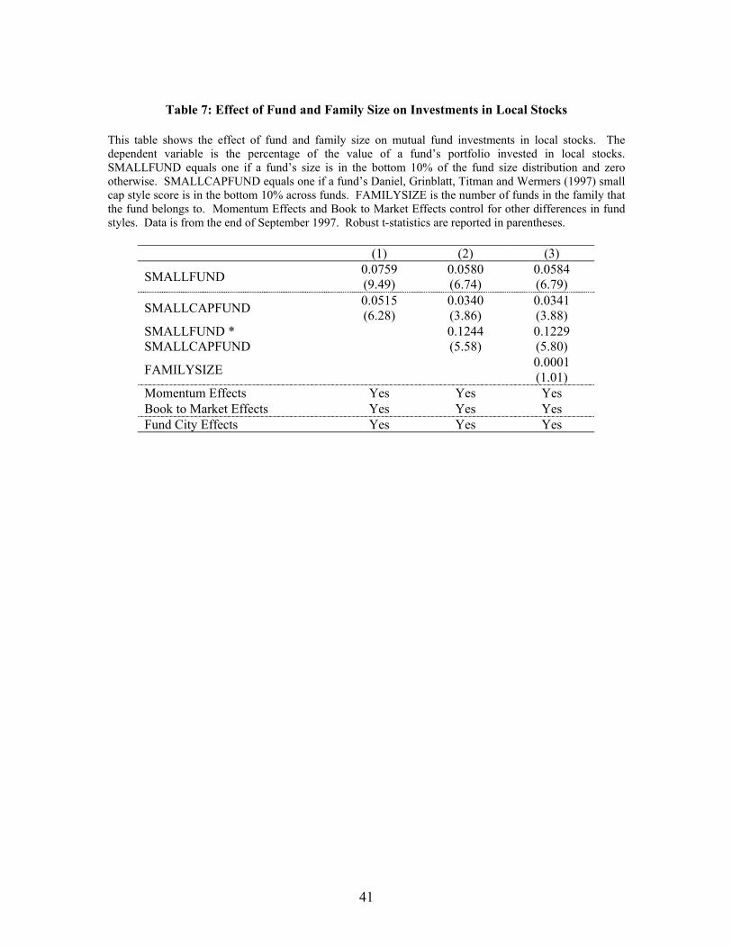
41

Table 7: Effect of Fund and Family Size on Investments in Local Stocks

This table shows the effect of fund and family size on mutual fund investments in local stocks. The dependent variable is the percentage of the value of a fund’s portfolio invested in local stocks. SMALLFUND equals one if a fund’s size is in the bottom 10% of the fund size distribution and zero otherwise. SMALLCAPFUND equals one if a fund’s Daniel, Grinblatt, Titman and Wermers (1997) small cap style score is in the bottom 10% across funds. FAMILYSIZE is the number of funds in the family that the fund belongs to. Momentum Effects and Book to Market Effects control for other differences in fund styles. Data is from the end of September 1997. Robust t-statistics are reported in parentheses.

(1) (2) (3)

SMALLFUND 0.0759 (9.49)

0.0580 (6.74)

0.0584 (6.79)

SMALLCAPFUND 0.0515 (6.28)

0.0340 (3.86)

0.0341 (3.88)

SMALLFUND * SMALLCAPFUND

0.1244 (5.58)

0.1229 (5.80)

FAMILYSIZE 0.0001 (1.01)

Momentum Effects Yes Yes Yes Book to Market Effects Yes Yes Yes Fund City Effects Yes Yes Yes

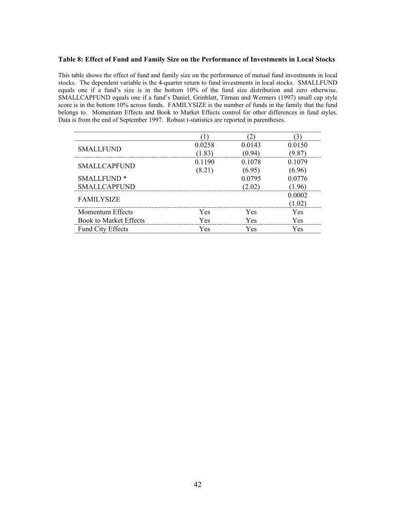
42

Table 8: Effect of Fund and Family Size on the Performance of Investments in Local Stocks This table shows the effect of fund and family size on the performance of mutual fund investments in local stocks. The dependent variable is the 4-quarter return to fund investments in local stocks. SMALLFUND equals one if a fund’s size is in the bottom 10% of the fund size distribution and zero otherwise. SMALLCAPFUND equals one if a fund’s Daniel, Grinblatt, Titman and Wermers (1997) small cap style score is in the bottom 10% across funds. FAMILYSIZE is the number of funds in the family that the fund belongs to. Momentum Effects and Book to Market Effects control for other differences in fund styles. Data is from the end of September 1997. Robust t-statistics are reported in parentheses.

(1) (2) (3)

SMALLFUND 0.0258 (1.83)

0.0143 (0.94)

0.0150 (9.87)

SMALLCAPFUND 0.1190 (8.21)

0.1078 (6.95)

0.1079 (6.96)

SMALLFUND * SMALLCAPFUND

0.0795 (2.02)

0.0776 (1.96)

FAMILYSIZE 0.0002 (1.02)

Momentum Effects Yes Yes Yes Book to Market Effects Yes Yes Yes Fund City Effects Yes Yes Yes