Does Capital Punishment Have a Deterrent Effect?New Evidence from Post-moratorium Panel Data*

Hashem DezhbakhshPaul H. Rubin

Joanna M. Shepherd

Department of EconomicsEmory University

Atlanta, Ga 30322-2240

January 2002

* We gratefully acknowledge helpful discussions with Issac Ehrlich and comments by BadiBaltagi, Robert Chirinko, Keith Hylton, David Mustard, George Shepherd, and participants in the1999 Law and Economic Association Meetings, 2000 American Economic Association Meetings,and workshops at Emory, Georgia State, Northwestern, and Purdue Universities. We are alsoindebted to Sam Peltzman for his valuable suggestions. The usual disclaimer applies.

Does Capital Punishment Have a Deterrent Effect?New Evidence from Post-moratorium Panel Data

Abstract

Evidence on the deterrent effect of capital punishment is important for many states that arecurrently considering a change in their position on the issue. We examine the deterrent hypothesisusing county-level post-moratorium panel data and a system of simultaneous equations. Theprocedure we employ overcomes the aggregation problem, eliminates the bias arising fromunobserved heterogeneity, and offers an inference which is relevant for the current crime level.Our results suggest that capital punishment has a strong deterrent effect. An increase in any of thethree probabilities— arrest, sentencing, or execution— tends to reduce the murder rate. Inparticular, each execution results, on average, in 18 fewer murders— with a margin of error of plusor minus 10. Tests show that results are not driven by “tough” sentencing laws, and are alsorobust to various specification choices. Our main finding, that capital punishment has a deterrenteffect, is fairly robust to choice of functional form (double-log, semi-log, or linear), state level vs.county level analysis, and sampling period.

1

I. Introduction

The acrimonious debate over capital punishment has continued for centuries (Beccaria, 1764,

and Stephen, 1864). In recent decades, the debate has heated up in the U.S. following the Supreme

Court-imposed moratorium on capital punishment.1 Currently, several states are considering a

change in their policies regarding the status of the death penalty. Nebraska’s legislature, for

example, recently passed a two year moratorium on executions, which was, however, vetoed by the

state’s governor. Ten other states have at least considered a moratorium last year (“Execution

Reconsidered,” The Economist, July 24th 1999, p 27). The group includes Oklahoma whose

legislature will soon consider a bill imposing a two year moratorium on executions and establishing

a task force to research the effectiveness of capital punishment. The legislature in Nebraska and

Illinois has also called for similar research. In Massachusetts, however, the House of

Representatives voted down a bill supported by the governor to reinstate the death penalty.

An important issue in this debate is whether capital punishment deters murders. Psychologists

and criminologists who examined the issue initially reported no deterrent effect (See, e.g., Sellin,

1959; Eysenck, 1970; and Cameron, 1994). Economists joined the debate with the pioneering work

of Ehrlich (1975, 1977). Ehrlich’s regression results, using U.S. aggregate time-series for 1933-

1969 and state level cross-sectional data for 1940 and 1950, suggest a significant deterrent effect,

which sharply contrasts with earlier findings. The policy importance of the research in this area is

borne out by the considerable public attention that Ehrlich’s work has received. The Solicitor

General of the United States, for example, introduced Ehrlich’s findings to the Supreme Court in

support of capital punishment.2

1 In 1972 the Supreme Court imposed a moratorium on capital punishment but in 1976 it ruled that executionsunder certain carefully specified circumstances are constitutional.2 Fowler vs. North Carolina, 428 U.S. 904 (1976).

2

Coinciding with the Supreme Court’s deliberation on the issue, Ehrlich’s finding inspired

an interest in econometric analysis of deterrence, leading to many studies that use his data but

different regression specifications— different regressors or different choice of endogenous vs.

exogenous variables.3 The mixed findings prompted a series of sensitivity analyses on Ehrlich’s

equations, reflecting a further emphasis on specification.4

Data issues, on the other hand, have received far less attention. Most of the existing studies

use either time-series or cross-section data. The studies that use national time-series data are

affected by an aggregation problem. Any deterrence from an execution should affect the crime rate

only in the executing state. Aggregation dilutes such distinct effects.5 Cross sectional studies are

less sensitive to this problem, but their static formulation precludes any consideration of the

dynamics of crime, law enforcement, and judicial processes. Moreover, cross sectional studies are

affected by unobserved heterogeneity which cannot be controlled for in the absence of time

variation. The heterogeneity is due to jurisdiction-specific characteristics that may correlate with

other variables of the model, rendering estimates biased. Several authors have expressed similar

data concerns or called for new research based on panel data.6 Such research will be timely and

useful for policy making.

We examine the deterrent effect of capital punishment using a system of simultaneous

equations and county-level panel data that cover the post-moratorium period. This is the most

disaggregate and detailed data used in this literature. Our analysis overcomes data and

3 See Cameron (1994) and Avio (1998) for literature summaries.4 Sensitivity analysis involves dividing the variables of the model into essential and doubtful and generatingmany estimates for the coefficient of each essential variable. The estimates are obtained from alternativespecifications each including some combination of the doubtful variables. See, e.g., Leamer (1983, 1985),McManus (1985), McAleer and Veall (1989), and Ehrlich and Liu (1999).5 For example, an increase in nonexecuting states’ murder rates aggregated with a drop in executing states’murder rate may incorrectly lead to an inference of no deterrence, as the aggregate data would show an increasein executions leading to no change in the murder rate.6 See, e.g., Hoenack and Weiler (1980), Cameron (1994), and Avio (1998).

3

econometric limitations in several ways. First, the disaggregate data allow us to capture the

demographic, economic, and jurisdictional differences among U.S. counties, while avoiding

aggregation bias. Second, by using panel data, we can control for some of unobserved

heterogeneity across counties, therefore avoiding the bias that arises from the correlation between

county-specific effects and judicial and law enforcement variables. Third, the large number of

county-level observations extends our degrees of freedom, thus broadening the scope of our

empirical investigation. The large data set also increases variability and reduces collinearity

among variables. Finally, using recent data makes our inference more relevant for the current

crime situation and more useful for the ongoing policy debate on capital punishment.

We, moreover, address two issues that appear to have remained in the periphery of the

specification debate in this literature. The first issue relates to the functional form of the

estimated equations. We bridge the gap between theoretical propositions concerning an

individual’s behavior and the empirical equation typically estimated at some level of

aggregation. An equation that holds true for an individual can also be applied to a county, state

or nation, only if the functional form is invariant to aggregation. This point is important when

similar equations are estimated at various levels of aggregation. The second issue relates to

murders that may not be deterrable— nonnegligent manslaughter and nonpremeditated crimes of

passion— that are included in commonly used murder data. We examine whether such inclusion

has an adverse effect on the deterrence inference. We draw on our discussions of these issues

and the specification debate in this literature to formulate our econometric model.

The paper is organized as follows: Section II reviews the literature on the deterrent effect of

capital punishment and outlines the theoretical foundation of our econometric model. Section III

describes data and measurement issues, presents the econometric specification, and highlights

4

important statistical issues. Section IV reports the empirical results and the corresponding analysis,

including an estimate of the number of murders avoided as the result of each execution. This section

also examines the robustness of our findings. Section V concludes the paper.

II. Capital Punishment and Deterrence

Historically, religious and civil authorities imposed capital punishment for many different

crimes. Opposition to capital punishment intensified during the European Enlightenment as

reformers such as Beccaria and Bentham called for abolition of the death penalty. Most Western

industrialized nations have since abolished capital punishment (for a list see Zimring and

Hawkins, 1986, chapter 1). The United States is an exception. In 1972, in Furman v. Georgia, the

Supreme Court outlawed capital punishment, arguing that execution was cruel and unusual

punishment, but in 1976, in Gregg v. Georgia, it changed its position by allowing executions

under certain carefully specified circumstances.7 There were no executions in the U.S. between

1968 and 1977. Executions resumed in 1977 and have increased steadily since then.

As Table 1 illustrates, from 1977 through 1999 there have been 598 executions in 31 states.

Six other states have adopted death penalty laws but have not executed anyone. Tennessee had

its first execution in April 2000, and twelve states do not have death penalty laws. Several of the

executing states are currently considering a moratorium on executions, while a few nonexecuting

states are debating whether to reinstate capital punishment.

The contemporary debate over capital punishment involves a number of important

arguments, drawing either on moral principles or social welfare considerations. Unlike morally-

based arguments which are inherently theoretical, welfare based arguments tend to build on

7 Furman v. Georgia, 408 U.S. 238 and Gregg v. Georgia, No. 74-6257, 428 U.S. 153; 96 S. Ct. 2909; 1976 U.S. Lexis82.

5

empirical evidence. The critical issue with welfare implications is whether capital punishment

deters capital crimes; an affirmative answer would imply that the death penalty can potentially

reduce such crimes. In fact, this issue is described as “the most important single consideration

for both sides in the death penalty controversy.”8

Ehrlich (1975, 1977) introduced regression analysis as a tool for examining the deterrent

issue. A plethora of economic studies followed Ehrlich’s. Some of these studies verbally

criticize or commend Ehrlich’s work, while others offer alternative analyses. Most analyses use

a variant of Ehrlich’s econometric model and his data (1933-1969 national time-series or 1940

and 1950 state level cross section). For example, Yunker (1976) finds a deterrent effect much

stronger than Ehrlich’s. Cloninger (1977) and Ehrlich and Gibbons (1977) lends further support

to Ehrlich’s finding. Bowers and Pierce (1975), Passel and Taylor (1977) and Hoenack and

Weiler (1980), on the other hand, find no deterrence when they use an alternative (linear)

functional form.9 Black and Orsagh (1978) find mixed results depending on the cross-section

year they use.

There are also studies that extend Ehrlich’s time-series data or use more recent cross-

sectional studies. Layson (1985) and Cover and Thistle (1988), for example, use an extension

of Ehrlich’s time-series data, covering up to 1977. Layson finds a significant deterrent effect of

executions, but Cover and Thistle who correct for data nonstationarity find no support for the

deterrent effect in general. Chressanthis (1989) uses time series data covering 1966 through

1985 and finds a deterrent effect. Grogger (1990) uses daily data for California during 1960-

1963 and finds no significant short-term correlation between execution and daily homicide rates.

8 Zimring and Hawkins (1986), p. 167.9 Ehrlich’s regression equations are in double-log form.

6

There are also a few recent studies. Brumm and Cloninger (1996), for example, who use

cross-sectional data covering 58 cities in 1985 report that the perceived risk of punishment is

negatively and significantly correlated with homicide commission rate. Lott and Landes (2000)

report a negative association between capital punishment and murder on a concurrent basis

when studying the effect of concealed handgun laws on public shootings. Cloninger and

Marchesini (2001) report that the Texas unofficial moratorium on executions during most of

1996 appears to have contributed to additional homicides. Mocan and Gittings (2001) find that

pardons may increase the homicide rate while executions reduce the rate. Zimmerman (2001)

also reports that executions have a deterrent effect.10 None of the existing studies, however, use

county level post-moratorium panel data.

Becker’s (1968) economic model of crime provides the theoretical foundation for much of

the regression analysis in this area. The model derives the supply, or production, of offenses for

an expected utility maximizing agent. Ehrlich (1975) extends the model to murders which he

argues are committed either as a by-product of other violent crimes or as a result of interpersonal

conflicts involving pecuniary or nonpecuniary motives.

Ehrlich derives several theoretical propositions predicting that an increase in perceived

probabilities of apprehension, conviction given apprehension, or execution given conviction will

reduce an individual’s incentive to commit murder. An increase in legitimate or a decrease in

illegitimate earning/income opportunities will have a similar crime-reducing effect.

Unfortunately, variables that can measure legitimate and illegitimate opportunities are not

readily available. Ehrlich and authors who test his propositions, therefore, use several economic

and demographic variables as proxies. Demographic characteristics such as population density,

10 We believe that the last two studies have econometric problems, but since these studies have not gone throughthe peer review process, discussing these problems would not be appropriate here.

7

age, gender, and race enter the analysis because earning opportunities (legitimate or illegitimate)

cannot be perfectly controlled for in an empirical investigation. Such characteristics may

influence earning opportunities, and can therefore serve as reasonable proxies.

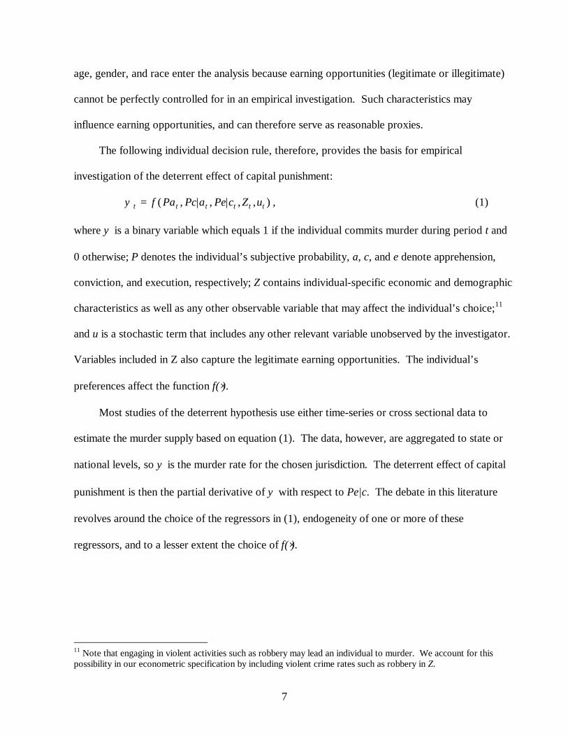
The following individual decision rule, therefore, provides the basis for empirical

investigation of the deterrent effect of capital punishment:

ψ t t t t t tf Pa Pc a Pe c Z u= ( , | , | , , ) , (1)

where ψ is a binary variable which equals 1 if the individual commits murder during period t and

0 otherwise; P denotes the individual’s subjective probability, a, c, and e denote apprehension,

conviction, and execution, respectively; Z contains individual-specific economic and demographic

characteristics as well as any other observable variable that may affect the individual’s choice;11

and u is a stochastic term that includes any other relevant variable unobserved by the investigator.

Variables included in Z also capture the legitimate earning opportunities. The individual’s

preferences affect the function f(⋅).

Most studies of the deterrent hypothesis use either time-series or cross sectional data to

estimate the murder supply based on equation (1). The data, however, are aggregated to state or

national levels, so ψ is the murder rate for the chosen jurisdiction. The deterrent effect of capital

punishment is then the partial derivative of ψ with respect to Pe|c. The debate in this literature

revolves around the choice of the regressors in (1), endogeneity of one or more of these

regressors, and to a lesser extent the choice of f(⋅).

11 Note that engaging in violent activities such as robbery may lead an individual to murder. We account for thispossibility in our econometric specification by including violent crime rates such as robbery in Z.

8

III. Model Specification and Data

In this section, we first address two data-related specification issues that have not received

due attention in the capital punishment literature. The first involves the functional form of the

econometric equations and the second concerns the allegedly adverse effect of including the

nondeterrable murders in the analysis. These discussions shape the formulation of our model.

A. Functional Form

Most econometric models that examine the deterrent effect of capital punishment derive

the murder supply from equation (1). The first step involves choosing a functional form for the

equation. Ideally, the functional form of the murder supply equation should be derived from the

optimizing individual’s objective function. Since this ideal requirement cannot be met in

practice, convenient alternatives are used instead. Despite all the emphasis that this literature

places on specification issues such as variable selection and endogeneity, studies often choose

the functional form of murder supply rather haphazardly.12 Common choices are double-log,

semi-log, or linear functions.

Rather than choosing arbitrarily one of these functional forms, we use the form that is

consistent with aggregation rules. More specifically, note that equation (1) purports to describe

the behavior of a representative individual. In practice, however, we rarely have individual level

data, and, in fact, the available data are usually substantially aggregated. Applying such data to

an equation derived for a single individual implies that the equation is invariant under

aggregation, and its extension to a group of individuals requires aggregation. For example, to

12 The only exceptions to this general observation are Hoenack and Weiler (1980), who criticize the use of adouble-log formulation suggesting a semi-log form instead, and Layson (1985), who uses Box-Coxtransformation as the basis for choosing functional form. Box-Cox transformation, however, is not appropriatefor the simultaneous equations model estimated here with panel data.

9

obtain an equation describing the collective behavior of the members of a group— e.g., residents

of a county, city, state, or country— one needs to add up the equations characterizing the

behavior of each member. If the group has n members, then n equations each with the same set

of parameters and the same functional form but different variables should be added up to obtain

a single aggregate equation. This aggregate equation has the same functional form as the

individual-level equation— it is invariant under aggregation— only in the linear case.

Because not every form has this invariance property, the choice of the functional form of

the equation is important,. For example, deterrence studies have applied the same double-log (or

semi-log) murder supply equation to city, state, and national level data, assuming implicitly that

a double-log (or semi-log) equation is invariant under aggregation. But this is not true because

the sum of n double-log equations would not be another double-log equation. A similar

argument rules out the semi-log specification.

The linear form, however, remains invariant under aggregation. Assume that the

individual’s murder supply equation (1) is linear in its variables,

ψ β β β γj t i i t i t i t j t t j ta Pa Pc a Pe c g Z TD u, , , , , ,| |= + + + + + +1 2 3 1 2 , (1′)

where j denotes the individual, i denotes county, ai is the county-specific fixed effect, TD is a set

of time trend dummies that captures national trends such as violent TV programming or movies

that have similar cross-county effects, and u’s are stochastic error terms with a zero mean and

variance σ2. Assume there are ni individuals in county i— for example, j=1,2,… ni— with

i=1,2,… .N, where N is the total number of counties in the U.S. Note that probabilities have an i

rather than a j subscript because only individuals in the same county face the same probability of

arrest, conviction, or execution.

10

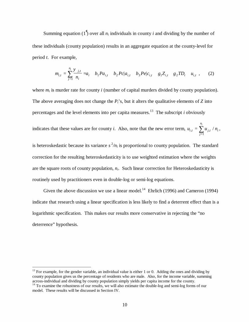
Summing equation (1′) over all ni individuals in county i and dividing by the number of

these individuals (county population) results in an aggregate equation at the county-level for

period t. For example,

mn

a Pa Pc a Pe c g Z TD ui tj t

ij

n

i i t i t i t i t t i t

i

,,

, , , , ,| |= = + + + + + +=∑ ψ

β β β γ1

1 2 3 1 2 , (2)

where mi is murder rate for county i (number of capital murders divided by county population).

The above averaging does not change the Pi’s, but it alters the qualitative elements of Z into

percentages and the level elements into per capita measures.13 The subscript i obviously

indicates that these values are for county i. Also, note that the new error term, u u ni t j tj

n

i

i

, , /==∑

1,

is heteroskedastic because its variance σ2/ni is proportional to county population. The standard

correction for the resulting heteroskedasticity is to use weighted estimation where the weights

are the square roots of county population, ni. Such linear correction for Heteroskedasticity is

routinely used by practitioners even in double-log or semi-log equations.

Given the above discussion we use a linear model.14 Ehrlich (1996) and Cameron (1994)

indicate that research using a linear specification is less likely to find a deterrent effect than is a

logarithmic specification. This makes our results more conservative in rejecting the “no

deterrence” hypothesis.

13 For example, for the gender variable, an individual value is either 1 or 0. Adding the ones and dividing bycounty population gives us the percentage of residents who are male. Also, for the income variable, summingacross-individual and dividing by county population simply yields per capita income for the county.14 To examine the robustness of our results, we will also estimate the double-log and semi-log forms of ourmodel. These results will be discussed in Section IV.

11

B. Nondeterrable Murders

Critics of the economic model of murder have argued that because the model cannot

explain the nonpremeditated murders, its application to overall murder rate is inappropriate. For

example, Glaser (1977) claims that murders committed during interpersonal disputes or

noncontemplated crimes of passion are not intentionally committed and are therefore

nondeterrable and should be subtracted out. Because the crime data include all murders without

a detailed classification, any attempt to exclude the allegedly nondeterrable crimes requires a

detailed examination of each reported murder and a judgement as to whether that murder can be

labeled deterrable or nondeterrable. Such expansive data scrutiny is virtually impossible.

Moreover, it would require an investigator to use subjective judgement, which would then raise

concerns about the objectivity of the analysis.

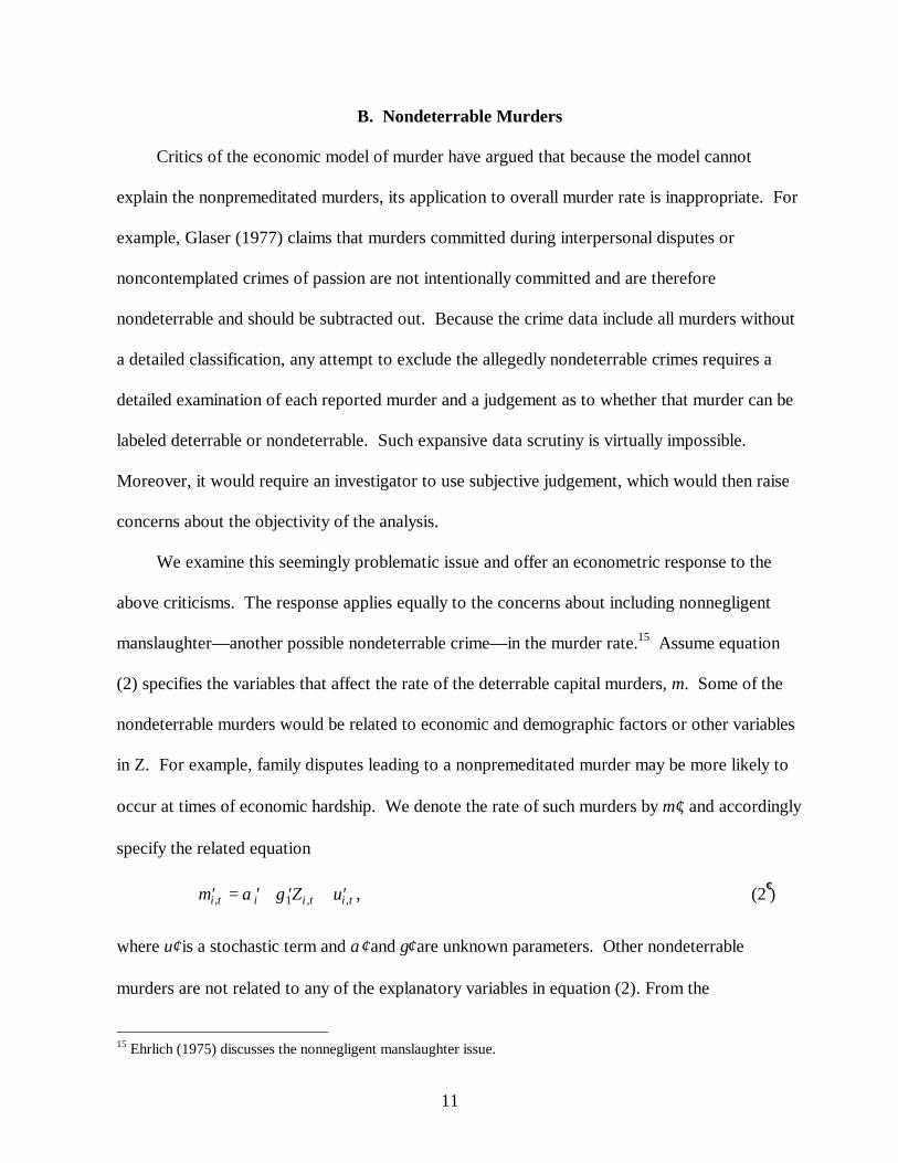
We examine this seemingly problematic issue and offer an econometric response to the

above criticisms. The response applies equally to the concerns about including nonnegligent

manslaughter— another possible nondeterrable crime— in the murder rate.15 Assume equation

(2) specifies the variables that affect the rate of the deterrable capital murders, m. Some of the

nondeterrable murders would be related to economic and demographic factors or other variables

in Z. For example, family disputes leading to a nonpremeditated murder may be more likely to

occur at times of economic hardship. We denote the rate of such murders by m′, and accordingly

specify the related equation

′= ′+ ′ + ′m Z ui t i i t i t, , ,α γ1 , (2′)

where u′ is a stochastic term and α′ and γ′ are unknown parameters. Other nondeterrable

murders are not related to any of the explanatory variables in equation (2). From the

15 Ehrlich (1975) discusses the nonnegligent manslaughter issue.

12

econometricians’ viewpoint, therefore, such murders appear as merely random acts. They

include accidental murders and murders committed by the mentally ill. We denote these by m′′,

and accordingly specify the related equation

′′= ′′+ ′′m ui t i i t, ,α , (2′′)

where u′′ is a stochastic term and α′′ is an unknown parameter. The overall murder rate is then

M=m+m′+m′′. which upon substitution for m′ and m′′ yields

M Pa Pc a Pe c Z TDi t i i t i t i t t i t, , , , ,| |= + + + + + +α β β β γ γ ε1 2 3 1 2 , (3)

where αι=aι+αι′+αι′′, γ1=g1+γ1′, and εi t i t i t i tu u u, , , ,= + ′+ ′′ is the compound stochastic term.16

Note that we cannot estimate g1, in equation (2), or γ1', in equation (2′), separately, because data

on separate murder categories are not readily available. This, however, does not prevent us from

estimating the combined effect γ1 , and neither does it affect our main inference which is about

the β’s.17 Therefore, any inference about the deterrent effect is unaffected by the inclusion of the

nondeterrable murders in the murder rate.

C. Econometric Model

The murder supply equation (3) provides the basis for our inference. The three subjective

probabilities in this equation are endogenous and need to be estimated through separate

equations. Endogeneity in this literature is often dealt with through the use of an arbitrarily

chosen set of instrumental variables. Hoenack and Weiler (1980) criticize earlier studies both

for this practice and for not treating the estimated equations as part of a theory-based system of

16 Note that the equation describing m'i,t may also include a national trend term (γ2′TDt). The term will beabsorbed into the coefficient of TD in equation (3).17 The added noise due to compounding of errors may reduce the precision of estimation, but it doe not affect thestatistical consistency of the estimated parameters.

13

simultaneous equations. We draw on the economic model of crime and the existing capital

punishment literature to identify a system of simultaneous equations.

We specify three equations to characterize the subjective probabilities in equation (3).

These equations capture the activities of the law enforcement agencies and the criminal justice

system in apprehending, convicting, and punishing perpetrators. Resources allocated to the

respective agencies for this purpose affects their effectiveness, and thus enters these equations.

The equations are

Pa M PE TDi t i i t i t t i t, , , , ,= + + + +φ φ φ φ ς1 2 3 4 , (4)

Pc a M JE PI PA TDi t i i t i t i t i t t i t| , , , , , , ,= + + + + + +θ θ θ θ θ θ ξ1 2 3 4 5 6 , (5)

Pe c M JE PI TDi t i i t i t i t t i t| , , , , , ,= + + + + +ψ ψ ψ ψ ψ ζ1 2 3 4 5 , (6)

where PE is police payroll expenditure, JE is expenditure on judicial and legal system, PI is

partisan influence as measured by the Republican presidential candidate’s percentage of the

statewide vote in the most recent election, PA is prison admission, TD is a set of time dummies

that capture national trends in these perceived probabilities, and ς , ξ, and ζ are error terms.

If police and prosecutors attempt to minimize the social costs of crime, they must balance

the marginal costs of enforcement with the marginal benefits of crime prevention. Police and

judicial/legal expenditure, PE and JE, represent marginal costs of enforcement. More

expenditure should increase the productivity of law enforcement or increase the probabilities of

arrest and conviction given arrest. Partisan influence is used to capture any political pressure to

get tough with criminals, a message popular with Republican candidates. The influence is

exerted through changing the makeup of the court system, such as the appointment of new

judges or prosecutors that are “tough on crime.” This affects the justice system and is, therefore,

included in equations (5) and (6). Prison admission is a proxy for the existing burden on the

14

justice system; the burden may affect judicial outcomes. This variable is defined as the number

of new court commitments admitted during each year.18 Also, note that all three equations

include county fixed effects to capture the unobservable heterogeneity across counties.

We use two other crime categories besides murder in our system of equations. These are

aggravated assault and robbery which are among the control variables in Z. Given that some

murders are the by-products of violent activities such as aggravated assault and robbery, we

include these two crime rates in Z when estimating equation (3). Forst, Filatov, and Klein

(1978) and McKee and Sesnowitz (1977) find that the deterrent effect vanishes when other crime

rates are added to the murder supply equation. They attribute this to a shift in the propensity to

commit crime which in turn shifts the supply function. We include aggravated assault and

robbery to examine this substitution effect.

The other control variables that we include in Z measure economic and demographic

influences. We include economic and demographic variables, which are all available at the

county-level, following other studies based on the economic model of crime.19 Economic

variables are used as proxy for legitimate and illegitimate earning opportunities. An increase in

legitimate earning opportunities increases the opportunity cost of committing crime, and should

result in a decrease in the crime rate. An increase in illegitimate earning opportunities increases

the expected benefits of committing crime, and should result in an increase in the crime rate.

Economic variables are real per capita personal income, real per capita unemployment insurance

payments, and real per capita income maintenance payments. The income variable measures

both the labor market prospects of potential criminals and the amount of wealth available to

18 This does not include returns of parole violators, escapees, failed appeals, or transfers.19 Inclusion of the unemployment rate which is available only at the state level does not affect the resultsappreciably.

15

steal. The unemployment payments variable is a proxy for overall labor market conditions and

the availability of legitimate jobs for potential criminals. The transfer payments variable

represents other nonmarket income earned by poor or unemployed people. Other studies have

found that crime responds to both measures of income and unemployment, but that the effect of

income on crime is stronger.

Demographic variables include population density, and six gender and race segments of the

population ages 10-29 (male, female; black, white, other). Population density is included to

capture any relationship between drug activities in inner cities and murder rate. The age, gender

and race variables represent the possible differential treatment of certain segments of the

population by the justice system, changes in the opportunity cost of time through the life cycle,

and gender/racially based differences in earning opportunities.

The control variables also include the state level National Rifle Association (NRA)

membership rate. NRA membership is included in response to a criticism of earlier studies.

Forst, Filatov, and Klein (1978) and Kleck (1979) criticize both Ehrlich and Layson for not

including a gun ownership variable. Kleck reports that including the gun variable eliminates the

significance of the execution rate. Also, all equations include a set of time dummies that capture

national trends and influences affecting all counties but varying over time.

D. Data and Estimation Method

We use a panel data set that covers 3,054 counties for the 1977-1996 period.20 More

current data are not available on some of our variables, because of the lag in posting data on law

20 We are thankful to John Lott and David Mustard for providing us with some of these data— from their 1997study— to be used initially for a different study (Dezhbakhsh and Rubin, 1998). We also note the data onmurder-related arrests for Arizona in 1980 is missing. As a result, we have to exclude from our analysis Arizonain 1980 (or 1982 and 1983 in cases where lags were involved). This will be explained further when we discussmodel estimation.

16

enforcement and judicial expenditures by the Bureau of Justice Statistics. The county-level data

allow us to include county-specific characteristics in our analysis, and therefore reduce the

aggregation problem from which much of the literature suffers. By controlling for these

characteristics, we can better isolate the effect of punishment policy.

Moreover, panel data allow us to overcome the unobservable heterogeneity problem that

affects cross-sectional studies. Neglecting heterogeneity can lead to biased estimates. We use

the time dimension of the data to estimate county fixed effects and condition our two stage

estimation on these effects. This is equivalent to using county dummies to control for

unobservable variables that differ among counties. This way we control for the unobservable

heterogeneity that arises from county specific attributes such as attitudes towards crime, or crime

reporting practices. These attributes may be correlated with the justice-system variables (or other

exogenous variables of the model) giving rise to endogeneity and biased estimation. An

advantage of the data set is its resilience to common panel problems such as self-selectivity,

nonresponse, attrition, or sampling design shortfalls.

We have county-level data for murder arrests which we use to estimate Pa. Conviction

data are not available, however, because the Bureau of Justice Statistics stopped collecting them

years ago. In the absence of conviction data, sentencing is a viable alternative that covers the

intervening stage between arrest and execution. This variable has not been used in previous

studies, although authors have suggested its use in deterrence studies (see, e.g., Cameron, 1994,

p. 210). We have obtained data from the Bureau of Justice Statistics on number of persons

sentenced to be executed by state for each year. We use this data along with arrest data to

estimate Pc|a. We also use sentencing and execution data to estimate Pe|c. Execution data are

17

at the state level because execution is a state decision. Expenditure variables in equations (4)-(6)

are also at the state level.

The crime and arrest rates are from the FBI’s Uniform Crime Reports.21 The data on age,

sex, and racial distributions, percent of state population voting Republican in the most recent

Presidential election, and the area in square miles for each county are from the U.S. Bureau of

the Census. Data on income, unemployment, income maintenance, and retirement payments are

obtained from the Regional Economic Information System. Data on expenditure on police and

judicial/legal systems, number of executions, and number of death row sentences, prison

populations, and prison admissions are obtained from the U.S. Department of Justice’s Bureau

of Justice Statistics. NRA membership rates are obtained from the National Rifle Association.

The model we estimate consists of the simultaneous system of equations (3)-(6). We use

the method of two stage least squares, weighted to correct for the Heteroskedasticity discussed

earlier. We choose two-stage over three-stage least squares because while the latter has an

efficiency advantage, it produces inconsistent estimates if an incorrect exclusionary restriction is

placed on any of the system equations. Since we are mainly interested in one equation— the

murder supply equation (3)— using the three-stage least squares method seems risky. Moreover,

the two-stage least squares estimators are shown to be more robust to various specification

problems.22 Other variables and data are discussed next.

21 The FBI Uniform Crime Report Data are the best county-level crime data currently available, in spite ofcriticisms about potential measurement issues due to underreporting. These criticisms are generally not sostrong for murder data that are central to our study. Nonetheless, there are safeguards in our econometricanalysis to deal with the issue. The inclusion of county-fixed effects eliminates the effects of time invariantdifferences in reporting methods across counties, and estimates of trends in crime should be accurate as long asreporting methods are not correlated across counties or time. Moreover, one way to address the problem ofunderreporting is to use the logarithms of crime rates, which are usually proportional to true crime rates. Ourgeneral finding is robust to introduction of logs as discussed in Section IV.22 See, e.g., Kennedy (1992, ch. 10).

18

IV. Empirical Results

A. Regression Results

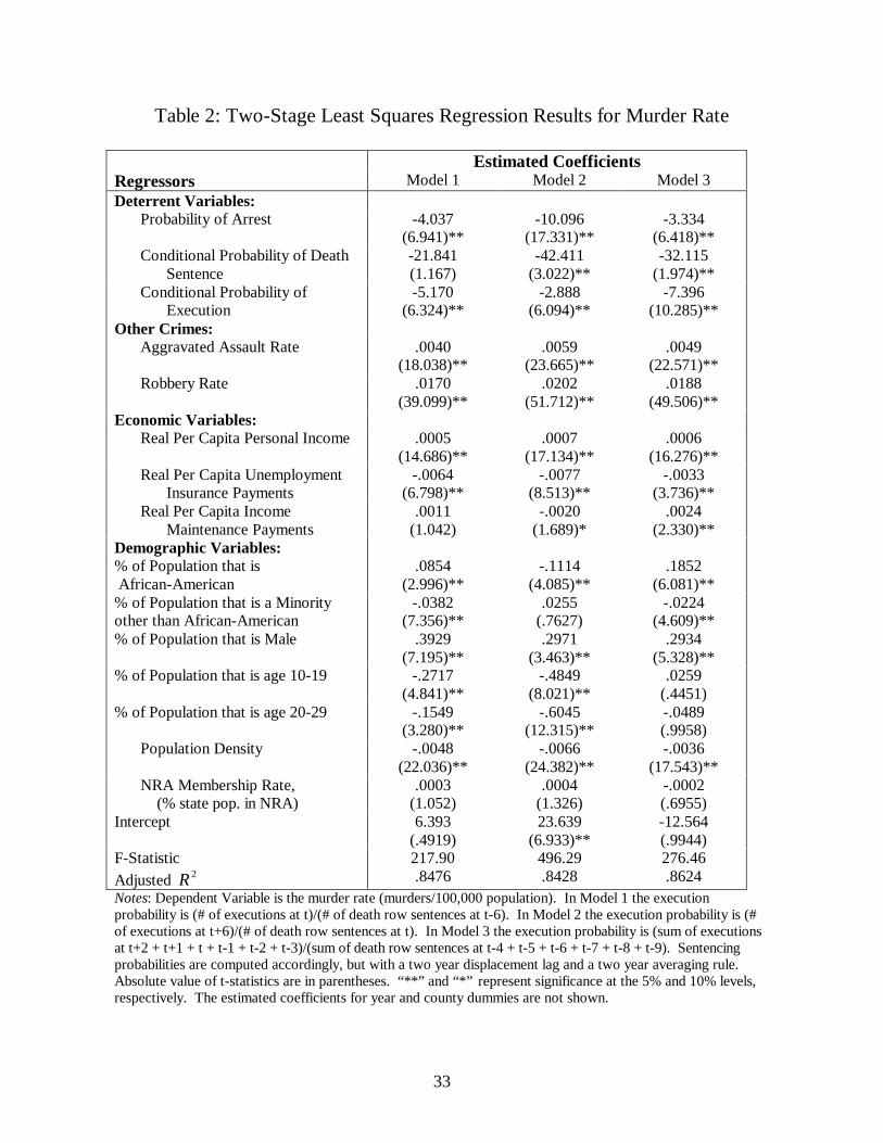
The coefficient estimates for the murder supply equation (3) obtained using the two-stage

least squares method and controlling for county-level fixed effects are reported in Tables 2 and

3.23 Various models reported in Tables 2 and 3 differ in the way the perceived probabilities of

arrest, sentencing and execution are measured. We first describe Table 2.

For model 1 in Table 2 the conditional execution probability is measured by executions at t

divided by number of death sentences at t− 6. For model 2 this probability is measured by

number of executions at t+6 divided by number of death sentences at t. The two ratios reflect

forward looking and backward looking expectations, respectively. The displacement lag of six

years reflects the lengthy waiting time between sentencing and execution, which averages six

years for the period we study (see Bedau ,1997, ch. 1). For probability of sentencing given arrest

we use a two year lag displacement, reflecting an estimated two year lag between arrest and

sentencing. Therefore, the conditional sentencing probability for model 1 is measured by the

number of death sentences at t divided by the number of arrests for murder at t− 2. For model 2

this probability is measured by number of death sentences at t+2 divided by number of arrests

for murder at t. Given the absence of an arrest lag, no lag displacement is used to measure the

arrest probability. It is simply the number of murder-related arrests at t divided by the number of

murders at t.

For model 3 in Table 2 we use an averaging rule. We use a six year moving average to

measure the conditional probability of execution given a death sentence. Specifically, this

23 Estimates of the coefficients of the other equations in the system are not reported, because we are mainlyinterested in equation (3) that provides direct inference about the deterrent effect. These estimates, however, areavailable from authors upon request.

19

probability at time t is defined as the sum of executions during (t+2, t+1, t, t-1, t-2, and t-3)

divided by the sum of death sentences issued during (t-4, t-5, t-6, t-7, t-8, and t-9). The six-year

window length and the six-year displacement lag capture the average time from sentence to

execution for our sample. In a similar fashion, a two-year lag and a two-year window length is

used to measure the conditional death sentencing probabilities. Given the absence of an arrest

lag, no averaging or lag displacement is used when computing arrest probabilities.24

Strictly speaking, these measures are not the true probabilities. However, they are closer to

the probabilities as viewed by potential murderers than would be the “correct” measures. Our

formulation is consistent with Sah’s (1991) argument that criminals form perceptions based on

observations of friends and acquaintances. We draw on the capital punishment literature to

parameterize these perceived probabilities,.

Models 4, 5, and 6 in Table 3 are, respectively, similar to models 1, 2 and 3 in Table 2

except for the way we treat undefined probabilities. When estimating the models reported in

Table 2, we observed that in several years some counties had no murders, and some states had no

death sentences. This rendered some probabilities undefined because of a zero denominator.

Estimates in Table 2 are obtained excluding these observations. Alternatively, and to avoid

losing data points, for any observation (county/year) where the probabilities of arrest or

execution are undefined due to this problem, we substituted the relevant probability from the

most recent year when the probability was not undefined. We look back up to four years,

because in most cases this eradicates the problem of undefined probabilities. The assumption

underlying such substitution is that criminals will use the most recent information available in

24 The absence of arrest data for Arizona in 1980, mentioned earlier, results in the exclusion of Arizona 1980from estimation of all three models, Arizona 1982 from estimation of models 2 and 3, and Arizona 1983 fromestimation of model 3.

20

forming their expectations. So a person contemplating committing a crime at time t will not

assume that he will not be arrested if no crime was committed, and hence no arrest was made,

during this period. Rather, he will form an impression of the arrest odds based on arrests in

recent years. This is consistent with Sah’s (1991) argument. Table 3 uses this substitution rule

to compute probabilities when they are undefined.

Results in Tables 2 and 3 suggest the presence of a strong deterrent effect. The estimated

coefficient of the execution probability is negative and highly significant in all six models. This

suggests that an increase in perceived probability of execution given that one is sentenced to

death will lead to a lower murder rate. The estimated coefficient of the arrest probability is also

negative and highly significant in all six models. This finding is consistent with the proposition

set forth by the economic models of crime that suggests an increase in the perceived probability

of apprehension leads to a lower crime rate.

For the sentencing probability, the estimated coefficients are negative in all models and

significant in three of the six models. It is not surprising that sentencing has a weaker deterrent

effect, given that we are estimating the effect of sentencing, holding the execution probability

constant. What we capture here is a measure of the “weakness’ or “porosity” of the state’s

criminal justice system. The coefficient of the sentencing probability picks up not only the

ordinary deterrent effect, but also the porosity signal. The latter effect may, indeed, be stronger.

For example, if criminals know that the justice system issues many death sentences but the

executions are not carried out, then they may not be deterred by an increase in probability of a

death sentence. In fact, an unpublished study by Leibman, Fagan and West reports that nearly

seventy percent of all death sentences issued between 1973 and 1995 were reversed on appeal at

the state or federal level. Also, six states sentence offenders to death but have performed no

21

executions. This reveals the indeterminacy of a death sentence and its ineffectiveness when it is

not carried out. Such indeterminacy affects the deterrence of a death sentence.

The murder rate appears to increase with aggravated assault and robbery, as the estimated

coefficients for these two variables are positive and highly significant in all cases. This is in part

because these crimes are caused by the same factors that lead to murder, and so measures of

these crimes serve as additional controls. In addition, this reflects the fact that some murders are

the byproduct of robbery or aggravated assault. In fact, several studies have documented that

increasing proportions of homicides are the outcome of robbery. (See, e.g., Zimring, 1977).

Additional demographic variables are included primarily as controls, and we have no

strong theoretical predictions about their signs. Estimated coefficients for per capita income are

positive and significant in all cases. This may reflect the role of illegal drugs in homicides

during this time period. Drug consumption is expensive, and may increase with income. Those

in the drug business are disproportionately involved in homicides because the business generates

large amounts of cash, which can lead to robberies, and because normal methods of dispute

resolution are not available. An increase in per capita unemployment insurance payments is

generally associated with a lower murder rate.

Other demographic variables are often significant. More males in a county is associated

with a higher murder rate, as is generally found (e.g., Daly and Wilson, 1988). An increase in

percentage of the teen-age population, on the other hand, appears to lower the murder rate. The

fraction of the population that is African American is generally associated with higher murder

rates, and the percentage that is minority other than African American is generally associated

with a lower rate.

22

The estimated coefficient of population density has a negative sign. One might have

expected a positive coefficient for this variable; murder rates are higher in large cities. However,

this may not be a consistent relationship: the murder rate can be lower in suburbs than it is in

rural areas, although rural areas are less densely populated than suburbs. But the murder rate

may be higher in inner cities where the density is higher than the suburbs.25 Glaeser and

Sacerdote (1999) also report that crime rates are higher for cities with 25,000-99,000 persons

than for cities with between 100,000-999,999 persons and then higher for cities over 1,000,000,

although not as high as for the smaller cities. (Glaeser and Sacerdote, 1999, Figure 3.) Because

there are relatively few counties containing cities of over 1,000,000, our measure of density may

be picking up this nonlinear relationship. They explain the generally higher crime rate in cities

as a function of higher returns, lower probabilities of arrest and conviction, and the presence of

more female headed households.

Finally, the estimates of the coefficient of the NRA membership variable are positive in

five of the six models and significant in half of the cases. A possible justification is that in

counties with a large NRA membership guns are more accessible, and they can therefore serve

as the weapon of choice in violent confrontations. The resulting increase in gun use, in turn,

may lead to a higher murder rate.

The most robust findings in these tables are as follows: The arrest, sentencing, and

execution measures all have a negative effect on murder rate, suggesting a strong deterrent effect

as the theory predicts. Other violent crimes tend to increase murder. The demographic variables

25 To examine the possibility of a piecewise relationship, we used two interactive (0 or 1) dummy variablesidentifying the low and the high range for density variable. The dummies were then interacted with the densityvariable. The estimated coefficient for models 1 through 3 were negative for the low density range and positivefor the high density range, suggesting that murder rate declines with an increase in population density forcounties that are not too densely populated, but increases with density for denser areas. This exercise did notalter the sign or significance of other estimated coefficients. For models 4-6, however, the interactive dummiesboth have a negative sign.

23

have mixed effects; murder seems to increase with the proportion of the male population .

Finally, the NRA membership variable has positive and significant estimated coefficients in all

cases, suggesting a higher murder rate in counties with a strong NRA presence.

B. Effect of Tough Sentencing Laws

One may argue that the documented deterrent effect reflects the overall toughness of the

judicial practices in the executing states. For example, these states may have tougher sentencing

laws that serve as a deterrent to various crimes including murder. To examine this argument, we

constructed a new variable measuring “judicial toughness” for each state,26 and estimated the

correlation between this variable and the execution variable. The estimated correlation

coefficient ranges from − .06 to .26 for the six measures of the conditional probability of

execution that we have used in our regression analysis. The estimated correlation between the

toughness variable and the binary variable that indicates whether or not a state has a capital

punishment law in any given year is .28.

We also added the toughness variable to equation (3), our main regression equation to see

whether its inclusion alters our results. The inclusion of the toughness variable did not change

the significance or sign of the estimated execution coefficient. Moreover, the toughness variable

has an insignificant coefficient estimate in four of the six regressions. The low correlation

between execution probability and the toughness variable, along with the observed robustness of

our results to inclusion of the toughness variable suggest that the deterrent finding is driven by

executions and not by tougher sentencing laws.

26 This variable takes values 0, 1, or 2 depending on whether a state has zero, one, or two tough sentencing lawsat a given year. The tough sentencing laws we consider are (i) truth-in-sentencing laws which mandate that aviolent offender must serve at least 85% of maximum sentence and (ii) “strikes” laws which significantlyincrease the prison sentences of repeat offenders. See, also, Mehlhop-Shepherd (2002a and b).

24

C. Magnitude of the Deterrent Effect

The statistical significance of the deterrent coefficients suggests that executions reduce the

murder rate. But how strong is the expected trade-off between executions and murders? In

other words, how many potential victims can be saved by executing an offender?27 Neither

aggregate time-series nor cross-sectional analyses can provide a meaningful answer to this

question. Aggregate time-series data, for example, cannot impose the restriction that execution

laws are state-specific and any deterrent effect should be restricted to the executing state. Cross-

sectional studies, on the other hand, capture the effect of capital punishment through a binary

dummy variable which measures an overall effect of the capital punishment laws instead of a

marginal effect.

Panel data econometrics provides the appropriate framework for a meaningful inference

about the trade-off. Here an execution in one state is modeled to affect the murders in the same

state only. Moreover, the panel allows estimation of a marginal effect rather than an overall

effect. To estimate the expected trade-off between executions and murder we can use estimates

of the execution deterrent coefficient ∃β3 as reported in Tables 2 and 3. We focus on Model 4 in

Table 3 which offers the most conservative (smallest) estimate of this coefficient. The

coefficient β3 is the partial derivative of murder per 100,000 population with respect to the

conditional probability of execution given sentencing (e.g., the number of executions at time t

divided by the number of death sentences issued at time t-6). Given the measurement of these

variables, the number of potential lives saved as the result of one execution can be estimated by

the quantity

27 Ehrlic (1975) and Yunker (1976) report estimates of such trade-offs using time-series aggregate data.

25

β3 (Populationt /100,000) (1/St-6) ,

where S is the number of individuals sentenced to death.

We evaluate this quantity for the U.S. using β3 estimate in Model 4 and t = 1996, the most

recent period that our sample covers. The resulting estimate is 18 with a margin of error of 10

and therefore a corresponding 95% confidence interval of (8 through 28).28 This implies that

each additional execution has resulted, on average, in 18 fewer murders, or in at least 8 fewer

murders. Also, note that the presence of population in the above expression is because murder

data used to estimate β3 is on a per capita basis. In calculating the trade-off estimate, therefore,

we use the population of the states with a death penalty law, since only residents of these states

can be deterred by executions.

D. Robustness of Results

While we believe that our econometric model is appropriate for estimating the deterrent

effect of capital punishment, the reader may want to know how robust are our results. To

provide such information, we examine the sensitivity of our main finding— that capital

punishment has a deterrent effect on capital crimes— to the econometric choices we have made.

In particular, we evaluate the robustness of our deterrence estimates to changes in aggregation

level, functional form, sampling period, modeling death penalty laws, and endogenous treatment

of the execution probability.

For each specification, we estimate the same six models as described above. The results

are reported in Table 4. Each row includes the estimated coefficient of the execution probability

(and the corresponding t-statistics) for the six models.29 Results are in general quite similar to

28 The 95% confidence interval is given by +(-)1.96[Standard Error of ( ∃β3 )](Populationt /100,000) (1/St-6)29 For brevity, we do not report full results which are available upon request.

26

those reported for the main specification. For example, using state-level data the estimated

coefficient of the execution probability is negative and significant in five of the six models,

suggesting a strong deterrent effect for executions. In the remaining case, model 4, the

coefficient estimate is insignificant.

We also estimate our econometric model in double-log and semi-log forms. These along

with the linear model are the commonly used functional forms in this literature. For the semi-

log form this coefficient estimate is negative and significant for all models but model 1 which

has a negative but insignificant coefficient. For the double-log form the estimated coefficient of

the execution probability is negative and significant in all six models. These result suggest that

our deterrence finding is not sensitive to the functional form of the model.

Given that the executions have accelerated in the 1990s, it is worthwhile to examine the

deterrent effect of capital punishment using only the 1990s data. This will also get at a possible

nonlinearity in the execution parameter. We, therefore, estimate models 1-6 using only the

1990s data. The coefficient estimate for the execution probability is negative and significant for

all models but model 2 which has a positive but insignificant coefficient.

As an additional robustness check we added to our linear model a dummy variable that

identifies the states with capital punishment. This variable takes a value of one if the state has a

death penalty law on the books in a given year, and zero otherwise. This variable allows us to

make a distinction between having a death penalty law and using it. The addition of this

variable did not change the sign or the significance of the estimated coefficient of the execution

probability. The estimated coefficient remains negative and significant in all six models. The

estimated coefficient of the dummy variable, on the other hand, does not show any additional

deterrence. This suggests that having a death penalty law on the books does not deter criminals

27

when the law is not applied. Finally, we estimated all six models reported in Tables 2 and 3

assuming that the execution probability is exogenous. In all six cases the estimated coefficient

of this variable turned out to be negative and significant, suggesting a strong deterrent effect.

Overall, we estimate 48 models; the estimated coefficient of the execution probability is

negative and significant in 45 of these models and insignificant in the remaining three models.

The above robustness checks suggest that our main finding that executions deter murders is not

sensitive to various specification choices.

V. Concluding RemarksDoes capital punishment deter capital crimes? The question remains of considerable interest.

Both presidential candidates in the Fall 2000 election were asked this question, and they both

responded vigorously in the affirmative. In his pioneering work, Ehrlich (1975, 1977) applied a

theory-based regression equation to test for the deterrent effect of capital punishment and reported

a significant effect. Much of the econometric emphasis in the literature following Ehrlich’s work

has been the specification of the murder supply equation. Important data limitations, however,

have been acknowledged.

In this study, we use a panel data set covering 3054 counties over the period 1977 through 1996

to examine the deterrent effect of capital punishment. The relatively low level of aggregation allows

us to control for county specific effects and also avoid problems of aggregate time-series studies.

Using comprehensive post-moratorium evidence, our study offers results that are relevant for

analyzing current crime levels and useful for policy purposes. Our study is timely because several

states are currently considering either a moratorium on executions or new laws to allow them to

execute criminals. In fact, the absence of recent evidence on the effectiveness of capital punishment

has prompted state legislatures in, for example, Nebraska to call for new studies on this issue.

28

We estimate a system of simultaneous equations in response to the criticism levied on studies

that use ad hoc instrumental variables. We use an aggregation rule to choose the functional form of

the equations we estimate: linear models are invariant to aggregation and are therefore the most

suited for our study. We also demonstrate that the inclusion of nondeterrable murders in murder

rate does not bias the deterrence inference.

Our results suggest that the legal change allowing executions beginning in 1977 has been

associated with significant reductions in homicide. An increase in any of the three probabilities

of arrest, sentencing, or execution tends to reduce the crime rate. Results are robust to

specification of such probabilities. In particular, our most conservative estimate is that the

execution of each offender seems to save, on average, the lives of 18 potential victims. (This

estimate has a margin of error of plus and minus 10). Moreover, we find robbery and aggravated

assault associated with increased murder rates. A higher NRA presence, measured by NRA

membership rate, seems to have a similar murder-increasing effect. Our main finding that

capital punishment has a deterrent effect is fairly robust to the choice of functional form (double-

log, semi-log, or linear), state level vs. county level analysis, sampling period. modeling

execution usage, and endogenous vs. exogenous execution probability. Overall, we estimate 48

models; the estimated coefficient of the execution probability is negative and significant in 45 of

these models and insignificant in the remaining three models.

Finally, a cautionary note is in order: deterrence reflects social benefits associated with the

death penalty, but one should also weigh in the corresponding social costs. These include the

regret associated with the irreversible decision to execute an innocent person. Moreover, issues

such as the possible unfairness of the justice system and discrimination need to be considered

when making a social decision regarding capital punishment.

29

ReferencesAndreoni, James (1995), “Criminal Deterrence in the Reduced Form: A New Perspective on

Ehrlich’s Seminal Study,” Economic Inquiry, 33, 476-83.

Avio, K.L. (1988), “Measurement Errors and Capital Punishment,” Applied Economics, 20,1253-1262.

Avio, K.L. (1998), “Capital Punishment,” in Peter Newman, editor, The New PalgraveDictionary of Economics and the Law, London: Macmillan Reference Limited.

Beccaria, C. (1764), On Crimes and Punishments, H. Puolucci (trans.), Indianapolis: Bobbs-Merrill.

Becker, Gary S. (1968), “Crime and Punishment: An Economic Approach,” Journal of PoliticalEconomy, 76, , 169-217.

Bedau Hugo A., ed. (1997), Death Penalty in America, Current Controversies, New York:Oxford University Press.

Black, T. and T. Orsagh (1978), “New Evidence on the Efficacy of Sanctions as a Deterrent toHomicide,” Social Science Quarterly, 58, 616-631.

Bowers, W.J. and J.L. Pierce, (1975), “The Illusion of Deterrence in Isaac Ehrlich’s work onCapital Punishment,” Yale Law Journal, 85: 187-208.

Brumm, Harold J. and Dale O. Cloninger (1996), “Perceived Risk of Punishment and theCommission of Homicides: A Covariance Structure Analysis,” Journal of EconomicBehavior and Organization, 31, 1-11.

Cameron, Samuel (1994), “A Review of the Econometric Evidence on the Effects of CapitalPunishment,” Journal of Socio-Economics, 23, 197-214.

Chressanthis, George A. (1989), “Capital Punishment and the Deterrent Effect Revisited: RecentTime-Series Econometric Evidence,” Journal of Behavioral Economics, Vol. 18, No. 2, 81-97.

Cloninger, Dale, O. (1977), “Deterrence and the Death Penalty: A Cross-Sectional Analysis,”Journal of Behavioral Economics, 6, 87-107.

Cloninger, Dale, O. and Roberto Marchesini (2001), “Execution and Deterrence: A Quasi-Controlled Group Experiment,” Applied Economics, Vol. 35, No. 5, 569-576.

Cover, James Peery and Paul D. Thistle (1988), “Time Series, Homicide, and the Deterrent Effectof Capital Punishment,” Southern Economic Journal, 54, 615-22.

Daly, Martin, and Margo Wilson (1988) Homicide, New York: Walter De Gruyter.

Dezhbakhsh, Hashem and Paul H. Rubin (1998), “Lives Saved or Lives Lost? The Effect ofConcealed-Handgun Laws on Crime, American Economic Review, Vol. 88, No. 2, May, 468-474.

Ehrlich, Isaac (1975), “The Deterrent Effect of Capital Punishment: A Question of Life andDeath,” American Economic Review Vol. 65, No. 3, June, 397-417.

30

Ehrlich, Isaac (1977) “Capital Punishment and Deterrence: Some Further Thoughts andAdditional Evidence,” Journal of Political Economy Vol. 85, August, 741-788.

Ehrlich, Isaac and Joel Gibbons (1977) “On the Measurement of the Deterrent Effect of CapitalPunishment and the Theory of Deterrence,” Journal of Legal Studies, Vol. 6, No. 1, 35-50.

Ehrlich, Isaac (1996), “Crime, Punishment, and the Market for Offenses,” Journal of EconomicPerspectives, Vol. 10, No. 1, Winter, 43-67.

Ehrlich, Isaac and Zhiqiang Liu (1999), “Sensitivity Analysis of the Deterrence Hypothesis: LetsKeep the Econ in Econometrics,” Journal of Law and Economics, Vol. 42, No. 1, April, 455-488.

Eysenck, H. (1970), Crime and Personality, London: Paladin.

Forst, B., V. Filatov ,and L.R. Klein, (1978), “The Deterrent Effect of Capital Punishment: AnAssessment of the Estimates,” in A. Blumstein, D. Nagin, & J. Cohen (editors), Deterrenceand Incapacitation: Estimating the Effects of Criminal Sanctions on Crime Rates,Washington, D.C.: National Academy of Sciences.

Glaeser, Edward L. and Bruce Sacerdote (1999), “Why is There More Crime in Cities,” Journalof Political Economy, Vol. 107, No. 6, 225-258.

Glaser, D. (1977), “The Realities of Homicide versus the Assumptions of Economists inAssessing Capital Punishment,” Journal of Behavioral Economics, 6: 243-268.

Grogger, Jeffrey (1990), “The Deterrent Effect of Capital Punishment: An Analysis of DailyHomicide Counts,” Journal of the American Statistical Association, Vol. 85, No. 410, June,295-303.

Hoenack, Stephen A. and William C. Weiler (1980), “A Structural Model of Murder Behaviorand the Criminal Justice System,” American Economic Review, 70, 327-41.

Kennedy, Peter (1992), A Guide to Econometrics, 3rd edition, Cambridge: The MIT Press.

Kleck, G. (1979), “Capital Punishment, Gun Ownership and Homicide,” American Journal ofSociology, 84, 882-910.

Layson, Stephen (1985), “Homicide and Deterrence: A Reexamination of the United StatesTime-Series Evidence,” Southern Economic Journal, Vol. 52, No. 1, July, 68-89.

Leamer, Edward (1983), “Let’s Take the Con out of Econometrics,” American Economic ReviewVol. 73, No. 1, March: 31-43.

Leamer, Edward (1985), “Sensitivity Analysis Would Help,” American Economic Review Vol.75, No. 3, June, 308-313.

Lott, John R. Jr. and David B. Mustard (1997), “Crime, Deterrence and Right-to-CarryConcealed Handguns,” Journal of Legal Studies Vol. 26, No. 1, 1-69.

Lott, John R., Jr. and William M. Landes (2000), “Multiple Victim Public Shootings,”University of Chicago Law and Economics Working Paper.

McAleer, Michael and Michael R. Veall (1989), “How Fragile are Fragile Inferences? A Re-evaluation of the Deterrent Effect of Capital Punishment,” Review of Economics andStatistics, 71, 99-106.

31

McKee, D.L., and M.L. Sesnowitz (1977), “On the Deterrent Effect of Capital Punishment,”Journal of Behavioral Economics, 6, 217-224.

McManus, W. (1985), “Estimates of the Deterrent Effect of Capital Punishment: The Importanceof the Researcher’s Prior Beliefs,” Journal of Political Economy, 93, 417-425.

Mehlhop-Shepherd, Joanna (2002a), “Fear of the First Strike: The Full Deterrent Effcet ofCalifornia’s Two- and Three-Strike Legislation,” Journal of Legeal Studies, Forthcoming.

Mehlhop-Shepherd, Joanna (2002b), “Police, Prosecutors, Criminals, and DeterminateSentencing: The Truth about Truth-in-Sentencing Laws,” The Journal of Law andEconomics, Forthcoming.

Mocan H. Naci and R. Kaj Gittings (2001), “Pardons, Executions, and Homisides,” University ofColorado, Unpublished Manuscript.

Passell, Peter and John B. Taylor (1977), “The Deterrent Effect of Capital Punishment: AnotherView,” American Economic Review, 67, 445-51.

Sah, Raaj K. (1991), “Social Osmosis and Patterns of Crime, Journal of Political Economy, Vol.99, No. 6, 1272-1295.

Sellin, J. T., (1959) The Death Penalty, Philadelphia: American Law Institute.

Stephen, J. (1864), “Capital Punishment,” Fraser’s Magazine, Vol. 69, 734-753.

Yunker, James A. (1976), “Is the Death Penalty a Deterrent to Homicide? Some Time SeriesEvidence, ”Journal of Behavioral Economics, Vol. 5, 45-81.

Zimmerman, Paul R. (2001), “Estimating the Deterrent Effect of Capital Punishment in thePresence of Endogeneity Bias,” Federal Communications Commission, Manuscript.

Zimring, Franklin E. (1977), “Determinants of the Death Rate From Robbery: A Detroit TimeStudy,” Journal of Legal Studies, Vol. 6, No 2, 317-332

Zimring, Franklin E. and Gordon Hawkins (1986), Capital Punishment and the AmericanAgenda, Cambridge: Cambridge University Press.

32

Table 1: Executions and Executing States

Year Number ofExecutions

Number of Stateswith Death

Penalty Laws1977 1 311978 0 321979 2 341980 0 341981 1 341982 2 351983 5 351984 21 351985 18 351986 18 351987 25 351988 11 351989 16 351990 23 351991 14 361992 31 361993 38 361994 31 341995 56 381996 45 381997 74 381998 68 381999 98 38

Notes: Of the 38 states with death penalty laws, Connecticut, Kansas, NewHampshire, New Jersey, New York, and South Dakota have yet to executeany death row inmates. Tennessee had its first execution in April of 2000.

33

Table 2: Two-Stage Least Squares Regression Results for Murder Rate

Estimated CoefficientsRegressors Model 1 Model 2 Model 3Deterrent Variables:

Probability of Arrest -4.037(6.941)**

-10.096(17.331)**

-3.334(6.418)**

Conditional Probability of DeathSentence

-21.841(1.167)

-42.411(3.022)**

-32.115(1.974)**

Conditional Probability ofExecution

-5.170(6.324)**

-2.888(6.094)**

-7.396(10.285)**

Other Crimes:Aggravated Assault Rate .0040

(18.038)**.0059

(23.665)**.0049

(22.571)**Robbery Rate .0170

(39.099)**.0202

(51.712)**.0188

(49.506)**Economic Variables:

Real Per Capita Personal Income .0005(14.686)**

.0007(17.134)**

.0006(16.276)**

Real Per Capita UnemploymentInsurance Payments

-.0064(6.798)**

-.0077(8.513)**

-.0033(3.736)**

Real Per Capita IncomeMaintenance Payments

.0011(1.042)

-.0020(1.689)*

.0024(2.330)**

Demographic Variables:% of Population that is African-American

.0854(2.996)**

-.1114(4.085)**

.1852(6.081)**

% of Population that is a Minorityother than African-American

-.0382(7.356)**

.0255(.7627)

-.0224(4.609)**

% of Population that is Male .3929(7.195)**

.2971(3.463)**

.2934(5.328)**

% of Population that is age 10-19 -.2717(4.841)**

-.4849(8.021)**

.0259(.4451)

% of Population that is age 20-29 -.1549(3.280)**

-.6045(12.315)**

-.0489(.9958)

Population Density -.0048(22.036)**

-.0066(24.382)**

-.0036(17.543)**

NRA Membership Rate, (% state pop. in NRA)

.0003(1.052)

.0004(1.326)

-.0002(.6955)

Intercept 6.393(.4919)

23.639(6.933)**

-12.564(.9944)

F-Statistic 217.90 496.29 276.46Adjusted 2R .8476 .8428 .8624Notes: Dependent Variable is the murder rate (murders/100,000 population). In Model 1 the executionprobability is (# of executions at t)/(# of death row sentences at t-6). In Model 2 the execution probability is (#of executions at t+6)/(# of death row sentences at t). In Model 3 the execution probability is (sum of executionsat t+2 + t+1 + t + t-1 + t-2 + t-3)/(sum of death row sentences at t-4 + t-5 + t-6 + t-7 + t-8 + t-9). Sentencingprobabilities are computed accordingly, but with a two year displacement lag and a two year averaging rule.Absolute value of t-statistics are in parentheses. “**” and “*” represent significance at the 5% and 10% levels,respectively. The estimated coefficients for year and county dummies are not shown.

34

Table 3: Two-Stage Least Squares Regression Results for Murder Rate

Estimated CoefficientsRegressors Model 4 Model 5 Model 6Deterrent Variables:

Probability of Arrest -2.264(4.482)**

-4.417(9.830)**

-2.184(4.568)**

Conditional Probability of DeathSentence

-3.597(.2475)

-47.661(4.564)**

-10.747(.8184)

Conditional Probability ofExecution

-2.715(4.389)**

-5.201(19.495)**

-4.781(8.546)**

Other Crimes:Aggravated Assault Rate .0053

(29.961)**.0086

(47.284)**.0064

(35.403)**Robbery Rate .0110

(35.048)**.0150

(54.714)**.0116

(41.162)**Economic Variables:

Real Per Capita Personal Income .0005(20.220)**

.0004(14.784)**

.0005(19.190)**

Real Per Capita UnemploymentInsurance Payments

-.0043(5.739)**

-.0054(7.317)**

-.0038(5.080)**

Real Per Capita IncomeMaintenance Payments

.0043(5.743)**

.0002(.2798)

.0027(3.479)**

Demographic Variables:% of Population that is African-American

.1945(9.261)**

.0959(4.956)**

.1867(7.840)**

% of Population that is a Minorityother than African-American

-.0338(7.864)**

-.0422(9.163)**

-.0237(5.536)**

% of Population that is Male .2652(6.301)**

.3808(8.600)**

.2199(4.976)**

% of Population that is age 10-19 -.2096(5.215)**

-.6516(15.665)**

-.1629(3.676)**

% of Population that is age 20-29 -.1315(3.741)**

-.5476(15.633)**

-.1486(3.971)**

Population Density -.0044(30.187)**

-.0041(27.395)**

-.0046(30.587)**

NRA Membership Rate, (% state pop. in NRA)

.0008(3.423)**

.0006(3.308)**

.0008(3.379)**

Intercept 10.327(.8757)

17.035(8.706)**

10.224(1.431)

F-Statistic 280.88 561.93 323.89Adjusted 2R .8256 .8062 .8269Notes: Dependent Variable is the murder rate (murders/100,000 population). In Model 4 the executionprobability is (# of executions at t)/(# of death row sentences at t-6). In Model 5 the execution probability is (#of executions at t+6)/(# of death row sentences at t). In Model 6 the execution probability is (sum of executionsat t+2 + t+1 + t + t-1 + t-2 + t-3)/(sum of death row sentences at t-4 + t-5 + t-6 + t-7 + t-8 + t-9). Sentencingprobabilities are computed accordingly, but with a two year displacement lag and a two year averaging rule.Absolute value of t-statistics are in parentheses. “**” and “*” represent significance at the 5% and 10% levels,respectively. The estimated coefficients for year and county dummies are not shown.

35

Table 4: Estimates of the Execuation Probability Coefficient Under VariousSpecifications (Robustness Check)

Specification Model 1 Model 2 Model 3 Model 4 Model 5 Model 6

State-Level Data − 5.343 − 2.257 − 6.271 − 1.717 − 4.046 − 2.895 (2.774)** (2.151)** (4.013)** (0.945) (6.486)** (1.867)*

Semi-Log − 0.145 − 0.191 − 0.218 − 2.715 − 5.201 − 4.781 (1.449) (3.329)** (2.372)** (4.389)** (19.495)** (8.546)**

Double Log − 0.155 − 0.078 − 0.144 − 0.150 − 0.181 − 0.158 (3.242)** (2.987)** (6.283)** (1.871)* (3.903)** (3.818)**

1990s Data − 3.021 0.204 − 3.251 − 1.681 − 4.079 − 2.791 (3.250)**) (0.301) (3.733)** (2.182)** (4.200)** (3.633)**

Execution Dummy Added

− 7.431 − 3.074 − 7.631 − 4.442 − 5.109 − 5.669 (9.821)** (6.426)** (11.269)** (7.143)** (19.564)** (9.922)**

Exogenous Execution Probability

− 0.494 − 0.428 − 2.515 − 0.309 − 0.377 − 1.761 (2.888)** (3.236)** (8.284)** (2.464)** (5.102)** (7.562)**

Notes: Absolute value of t-statistics are in parentheses. “**” and “*” represent significance at the 5% and10% levels, respectively. The estimated coefficients for the other variables are available upon request. See,also, notes to Tables 2 and 3.