Electronic copy available at: http://ssrn.com/abstract=2156623

Does Academic Research Destroy Stock Return Predictability?*

R. David McLean

University of Alberta and MIT Sloan School of Management

Phone: 774-270-2300

Email: rdmclean@MIT.edu

Jeffrey Pontiff

Boston College

Phone: 617-552-6786

Email: pontiff@bc.edu

January 23, 2013

Abstract

We study the out-of-sample and post-publication return-predictability of 82 characteristics that are identified in published academic studies. The average out-of-sample decay due to statistical bias is about 10%, but not statistically different from zero. The average post-publication decay, which we attribute to both statistical bias and price pressure from aware investors, is about 35%, and statistically different from both 0% and 100%. Our findings point to mispricing as the source of predictability. Consistent with informed trading, after publication, stocks in characteristic portfolios experience higher volume, variance, and short interest, and higher correlations with portfolios that are based on published characteristics. Consistent with costly (limited) arbitrage, post-publication return declines are greater for characteristic portfolios that consist of stocks with low idiosyncratic risk. Keywords: Return predictability, limits of arbitrage, publication impact, market efficiency, comovement, statistical bias. JEL Code: G00, G14, L3, C1

                                                            * We are grateful to the Q Group and the Dauphine-Amundi Chair in Asset Management for financial support. We thank participants at the Financial Research Association’s 2011 early ideas session, seminar participants at Babson College, Brandeis University, Boston College, CKGSB, HBS, Georgia State, HEC Montreal, MIT, Northeastern, University of Toronto, University of Maryland, City University of Hong Kong International Conference, Finance Down Under Conference 2012, University of Georgia, University of Washington Summer Conference, European Finance Association (Copenhagen), 1st Luxembourg Asset Management Conference, and Turan Bali, Shane Corwin, Mark Bradshaw, Alex Edmans, Lian Fen, Bruce Grundy, Pierluigi Balduzzi, David Chapman, Wayne Ferson, Francesco Franzoni, Xiaohui Gao, Thomas Gilbert, Clifford Holderness, Darren Kisgen, Owen Lamont, Jay Ritter, Robin Greenwood, Paul Schultz, Bruno Skolnik, Jeremy Stein, Matti Suominen, Allan Timmermann, Michela Verado, Artie Woodgate, and Jianfeng Yu for helpful conversations.

Electronic copy available at: http://ssrn.com/abstract=2156623

 

1  

Finance research has uncovered many cross-sectional relations between predetermined

variables and future stock returns. Beyond historical curiosity, these relations are relevant to the

extent that they provide insight into the future. Whether or not the typical relation continues

outside of the study’s original sample is an open question, the answer to which can shed light on

why cross-sectional return predictability is observed in the first place.1 Although several papers

note whether a specific cross-sectional relation continues, low statistical power prevents

meaningful comparisons among in-sample returns, post-sample returns, and post-publication

returns. Moreover, previous studies often produce contradictory messages. As examples,

Jegadeesh and Titman (2001) show that the relative returns to high momentum stocks increased

after the publication of their original paper, while Schwert (2003) argues that post-publication,

the value and size effects have disappeared, and Green, Hand, and Solimon (2011) show that the

accrual effect has disappeared. A handful of studies look at more than one characteristic, but they

do not use post-sample or post-publication dates to make clear comparisons, and they also

produce contradictory messages.2

In this paper we synthesize information from 82 characteristics that have been shown to

explain cross-sectional stock returns in peer-reviewed finance, accounting, and economics

journals. Our goal is to better understand what happens to return-predictability outside of a

study’s sample period. We compare each characteristic’s return-predictability over three distinct

periods: (i) the original study’s sample period; (ii) after the original sample period but before

                                                            1 We focus on cross-sectional variables. For an analysis of the performance of time-series variables, see

LeBaron (2000) and Goyal and Welch (2008). For an analysis of calendar effects, see Sullivan, Timmermann, and White (2011).

2 For example, Lewellen (2011) uses 15 variables to produce a singular rolling cross-sectional return proxy and shows that it predicts, with decay, next period’s cross section of returns. Haugen and Baker (1996) and Chordia, Subrahmanyan, and Tong (2011) compare characteristics in two separate subperiods. Haugen and Baker show that each of their characteristics produces statistically significant returns in the second-subsample, whereas Chordia, Subrahmanyan, and Tong show that none of their characteristics is statistically significant in their second-subsample. Green, Hand, Zhang (2012) identify 300 published and unpublished characteristics but they do not estimate characteristic decay parameters as a function of publication or sample-end dates.

Electronic copy available at: http://ssrn.com/abstract=2156623

 

2  

publication; and (iii) post publication. Previous studies contend that return-predictability is either

the outcome of a rational asset pricing model, or statistical biases, or mispricing. By comparing

return-predictability across our three distinct periods, we are able to give insight into what best

explains the typical characteristic’s return-predictability.

Pre-publication, out-of-sample predictability. If return-predictability in published studies

is the result of statistical biases, then predictability should disappear out of sample, even before

the paper is published. We use the term “statistical biases” to describe a broad array of biases

that are inherent to published research.

We know of at least four types of statistical biases that could affect stock return-

predictability. Leamer (1978) investigates the impact of “specification search” biases. These

biases occur if the choice of model is influenced by the model’s result. Lo and MacKinlay

(1990) examine a specific type of specification search bias found in finance, which they refer to

as the “data snooping bias.” This effect arises when researchers form portfolios to show that a

characteristic is related to future returns, and the choice of how the portfolios are formed is

affected by the return-predictability of the portfolio. A second type of bias is sample selection

bias, studied in Heckman (1979), where the sample construction is influenced by the result of

the test. A third type of bias, considered by Hedges (1992), is that the likelihood of publication is

correlated with the magnitude of the study’s test statistic. Fama (1991) describes a publication

bias, when he notes that, “With clever researchers on both sides of the efficiency fence,

rummaging for forecasting variables, we are sure to find instances of ‘reliable’ return

predictability that are in fact spurious.” A fourth type of bias can occur if a strategy’s spuriously

high returns attract academic attention to the strategy, making the publication date endogenous.3

                                                            3 We thank Allan Timmermann for pointing out this possibility.

 

3  

To the extent that the results in these studies are caused by such biases, we should observe a

decline in return-predictability out of sample.

Post-publication predictability. The literature makes conflicting predictions about post-

publication predictability. At one extreme, publication may be unrelated to return predictability.

Cochrane (1999) explains that if predictability reflects risk, then it is likely to persist regardless

of how many people know about it: “Even if the opportunity is widely publicized, investors will

not change their portfolio decisions, and the relatively high average return will remain.”

Cochrane’s argument follows Muth’s (1961) rational expectations hypothesis, and thus the logic

can be broadened to non-risk models such as Amihud and Mendelson’s (1986) transaction-based

model and Brennan’s (1970) tax-based model. These frameworks assume that agents are rational,

and suggest that publication should not affect the perceived risks and costs that drive the

expected returns. If Cochrane’s and Muth’s conjectures are true, pre- and post-publication (and

out-of-sample but pre-publication) return-predictability should be similar.4

At the other extreme, if return-predictability is entirely the result of mispricing, and if

publication draws the attention of sophisticated investors who trade against the mispricing, then

we might expect the effects to disappear after the paper is published. This framework is proposed

in Schwert (2003), who argues that argues: “the activities of practitioners who implement

strategies to take advantage of anomalous behavior can cause the characteristics to disappear.”5

We can differentiate this effect from that of statistical biases by finding a greater decline post-

publication as compared to any decline out of-sample but pre-publication.

                                                            4 This logic can be extended to irrational return predictability as well. Industry research may lead academic

research, such that the information in academic publications is redundant to market participants. 5 To our knowledge, the first empirical examination of the effects of academic research on capital markets

is Mittoo and Thompson’s (1990) study of the size effect. They use a regime switching model to illustrate a post-1983 difference in returns to size portfolios.

 

4  

Others contend that practitioners will not trade enough to fully eradicate return-

predictability resulting from mispricing. Rather, mispricing may continue at a reduced level.

Delong, Shleifer, Summers, and Waldman (1990) show than systematic noise trader risk may

allow mispricing to continue. Pontiff (1996, 2006) shows that other arbitrage costs, and in

particular holding costs associated with idiosyncratic risk, can prevent sophisticated trades from

entirely eliminating mispricing.6 Shleifer and Vishny (1997) point out that these effects are

greater if arbitrageurs are agents who are evaluated by uninformed principals who confuse

volatility with performance.

Although in the long-run, mispricing-induced predictability is expected to either disappear

(Schwert, 2003), or at least decay (Pontiff, 1996, and Shleifer and Vishny, 1997), in the short-run

it may become more pronounced. This may occur if characteristics are persistent. In this case,

when sophisticated investors learn of predictability, they increase allocations to positions that are

expected to earn the highest returns. This creates price pressure that results in even higher returns

than would have occurred in the absence of the publication. The higher returns are a temporary

reaction. Since mispricing is reduced, long-run returns will be lower.

Findings. We conduct our analysis using 82 different characteristics from 68 different

studies. The period during which a characteristic is outside of its original sample but still pre-

publication, is useful for estimating the effects of statistical biases. We find that on average,

return-predictability declines by 10% during this period. This suggests an upper-bound estimate

on the effect of statistical biases to be about 10%. Thus, an in-sample finding that implies a 5%

alpha is expected to produce a bias-free alpha of at least 4.5%. This finding is statistically

insignificant—we cannot reject the hypothesis that there are no statistical biases. Our 10%

estimate is likely to be too high, since we expect some traders learn about of the characteristic                                                             

6 For further evidence of this effect see Duan, Hu, and McLean (2009 and 2010) and McLean (2010) 

 

5  

predictability before publication—perhaps through workshop and conference presentations, and

their actions will cause some decay that we attribute to statistical biases.

We estimate that the average characteristic’s return decays by about 35% post-publication.

Thus, an in-sample alpha of 5% is expected to decay to 3.25% post-publication. We attribute this

effect due to both statistical biases, and to the activity of sophisticated traders who observe the

publication. Combining this finding with an estimated statistical bias of 10% implies a lower

bound on the publication effect of about 25%. We can reject the hypothesis that post-publication

return-predictability does not change, and we can reject the hypothesis that there is no post-

publication alpha. These findings are robust to replacing publication date with Social Science

Research Network (SSRN) posting date, and they do not appear to be caused by time trends in

characteristic returns.

We further investigate the effects of publication by studying traits that reflect trading

activity. We find that within characteristic portfolios, variance, turnover, and dollar volume all

increase post-publication. The difference in the relative amount of short interest between the

short and long sides of each characteristic-portfolio also increases after publication. These

findings are all consistent with the idea that mispricing is the source of characteristic-based

cross-sectional predictability, and that academic research draws attention to characteristics,

which in turn increases trading in the stocks with the largest expected return differentials.

We also find that during the original sample period, stocks on the short side of a

characteristic tend to be more highly shorted than stocks on the long side. This could reflect the

fact that some practitioners knew that the characteristics predicted stock returns before

academics did. Alternatively, it could be that practitioners were unaware of the characteristic’s

predictive power, but instead took positions based on firm-specific or other analyses, and these

 

6  

positions turned out to be correlated with the characteristic.7 The difference in the amount of

shorting between the short and long sides of each characteristic increases by a factor of nine after

a paper has been published, so even if some practitioners knew of the strategy before the paper

was published, many more seem to know afterwards.

Across characteristics, the post-publication decline is greatest for characteristics that

require more trading in stocks with high market values, high liquidity, low idiosyncratic risk, and

in stocks that pay dividends. As we mention above, Pontiff (1996 and 2006), and Shleifer and

Vishny (1997) point out that costs and risks associated with arbitrage could prevent mispricing

from being completely eliminated. Hence, our findings are consistent with mispricing being the

source of characteristic return-predictability: publication draws the attention of arbitrageurs, and

the post-publication returns decline the most for portfolios that are the least costly to arbitrage.

Surprisingly, measures that proxy for the attractiveness of the strategy, such as the in-sample

Sharpe ratio and the in-sample t-statistic do not forecast post-publication decay. Similarly, a

proxy for systematic risk, which should distinguish cross-sectional predictability that is the result

of rational asset pricing from predictability that is the result of mispricing, is associated with

larger (albeit insignificant) declines in predictability.

Our final investigation is whether academic publication is associated with changes in

covariance between characteristics. We find that yet-to-be-published characteristic portfolios are

correlated, however, after a characteristic is published, its correlation with other yet-to-be-

published characteristic portfolios decreases, while its correlation with other already-published

characteristic portfolios increases. One interpretation of this finding is that characteristics are the

                                                            7 As an example, some investors try to find undervalued stocks by studying the fundamentals of individual

companies. Such an investor, who goes long stocks that appear to be undervalued, and short stocks that appear to be overvalued, will probably end up long in stocks with high book-to-market ratios, and short in stocks with low book-to-market ratios, even though the investor is not choosing stocks based on book-to-market ratios.

 

7  

result of mispricing, and mispricing has a common source; this is why in-sample characteristic

portfolios are correlated. This interpretation is consistent with the irrational comovement models

proposed in Lee, Shleifer, and Thaler (1991) and Barberis and Shleifer (2003). Publication then

causes more arbitrageurs to trade on the characteristic, which causes characteristic portfolios to

become more correlated with already-published characteristic portfolios that are also pursued by

arbitrageurs, and less correlated with yet-to-be-published characteristic portfolios.

1. Research Method

We identify studies that find cross-sectional relations between variables that are known in a

given month and stock returns in the following month(s). We do not study time series

predictability. We limit ourselves to studies in the academic peer-reviewed finance and

accounting literatures where the null of no cross-sectional predictability is rejected at the 5%

level, and to studies that can be constructed with publicly available data. Most often, these

studies are identified with search engines such as Econlit by searching for articles in finance and

accounting journals with words such as “cross-section.” Some studies are located from reference

lists in books or other papers. Lastly, in the process of writing this paper, we contacted other

finance professors and inquired about cross-sectional relations that we may have missed.

Most studies that we identify either demonstrate cross-sectional predictability with Fama-

MacBeth (1973) slope coefficients or with long-short portfolio returns. Some of the studies that

we identify demonstrate a univariate relation between the characteristic and subsequent returns,

while other studies include additional control variables. Some studies that we identify are not

truly cross-sectional, but instead present event-study evidence that seems to imply a cross-

 

8  

sectional relation. Since we expect the results from these studies to provide useful information to

investors, we also include them in our analyses.

We use 82 cross-sectional relations from 68 different studies. We include all variables that

relate to cross-sectional returns, including those with strong theoretical motivation such as Fama

and MacBeth’s landmark 1973 study of market beta in the Journal of Political Economy and

Amihud’s 2002 study of a liquidity measure in the Journal of Financial Markets. The study with

the most number of original cross-sectional relations that we utilize (4) is Haugen and Baker’s

1996 study of cross-section stock returns in the Journal of Financial Economics. Haugen and

Baker (1996) investigate more than four cross-sectional relations, but some of these relations

were documented by other authors earlier, and are therefore associated with other publications in

our study. The first study in our sample is Blume and Husic’s 1972 Journal of Finance study of

how price level relates to future stock returns. The most recent study is Bali, Cakici, and

Whitelaw’s 2011 Journal of Financial Economics study that shows that the maximum daily

return that a security experiences in the preceding month predicts the next period’s monthly

return.

We are unable to exactly construct all of the characteristics. In such cases, we calculate a

characteristic that captures the intent of the study. As examples, Franzoni and Marin (2006) show

that a pension funding variable predicts future stock returns. This variable is no longer covered

by Compustat, so we use available data from Compustat to construct a variable that we expect to

contain much of the same information. Dichev and Piotroski (2001) show that firms that are

downgraded by Moody’s experience negative future abnormal returns. Compustat does not cover

Moody’s ratings, but it does cover S&P ratings, and so we use S&P rating downgrades instead.

Characteristics that use accounting data are winsorized, such that values that are below the 1st

 

9  

percentile are assigned the value of the 1st percentile, and values that are above the 99th

percentile are assigned the value of the 99th percentile.

We estimate each characteristic’s return predictability using two different methods. First,

we calculate monthly Fama-MacBeth (1973) slope coefficient estimates using a continuous

measure of the characteristic (e.g. firm size or past returns). As Fama (1976) shows, Fama-

MacBeth slope coefficients are returns from long-short portfolios with unit net exposure to the

characteristic. Second, we calculate the return of a portfolio that each month invests in stocks in

the top 20th percentile of the characteristic minus the return of a portfolio that invests in stocks in

the bottom 20th percentile of the characteristic. We report our basic findings using both methods.

2. Creating the Data and In-Sample Replicability

Summary statistics for the characteristics that we study are provided in Table 1. We define

the publication date as the date based on the journal’s year and issue. For this date convention,

the average length of time between the end of the sample and publication is 55 months. For

comparison, the average original in-sample span is 323 months, and the average out-of-sample

span is 139 months. As a robustness check, we also consider the publication date to be the earlier

of the actual publication date and the first time that paper appeared on the SSRN. The average

number of months between the end of the sample and SSRN date is 44 months.

As we mention previously, for all characteristics we calculate monthly Fama-MacBeth

slope coefficients using continuous measures of the characteristic (e.g., size or past returns).

Fifteen of our 82 characteristics involve binary variables, such as dividend initiation (Michaely,

Thaler, and Womack, 1995). For all characteristics that do not involve a binary characteristic, we

also calculate the long-short portfolio monthly return using extreme quintiles. Returns are

 

10  

equally weighted unless the primary study presents value-weighted portfolio results (e.g., Ang,

Hodrick, Xing, and Zhang, 2006, and Bali and Cakici, 2008).

Our goal is not to perfectly replicate a paper. This is impossible since CRSP data changes

over time and papers often omit details about precise calculations. Ten of our average in-sample

Fama-MacBeth slope coefficients produce t-statistics that are between -1.50 and 1.50.8 We do

not include these characteristics in the paper’s main tests. Thus, a total of 72 (82 – 10)

characteristics are used in the paper’s primary tests.

Admittedly, the decision to use a t-statistic cut-off of 1.50 is arbitrary. The decision was

motivated by a desire to utilize as many characteristics as possible, while still measuring the

same essential characteristic as the original paper. Given that some papers feature characteristics

with t-statistics that are close to 2.0 and that we are not perfectly replicating the original authors’

methodology, a cut-off of 1.50 seemed reasonable to us. That stated, only two of the 72

characteristics that we include in the paper’s analyses have t-statistics that are less than 1.80.

2.1. Preliminary Findings

Table 2 reports characteristic-level summary statistics regarding the out-of-sample and post

publication return-predictability of the 72 predictors that we were able to replicate. To be

included in the tests in this table, we require that a characteristic portfolio have at least 36

monthly observations during the measurement period (e.g., post-publication). We relax this

restriction in our pooled regression tests, which weight each characteristic-month observation

equally, rather than each characteristic.

                                                            8 If a characteristic is not associated with a t-statistic outside of the -1.50 to 1.50 range, both co-authors

independently wrote code to estimate the effect.

 

11  

To estimate the statistics in Table 2, we first calculate the in-sample mean for each

characteristic-portfolio, as described in the previous section. We then scale the monthly out-of-

sample and post-publication portfolios by the in-sample means. We use the scaled values to

generate statistics that reflect the average out-of-sample and post-publication return of each

portfolio relative to its in-sample mean. We generate individual statistics for each characteristic-

portfolio and then take a simple average across all of the characteristics. We do this for the

continuous version of each characteristic-portfolio (Panel A), the quintiles version (Panel B), and

the strongest form (continuous vs. quintile) (Panel C).

As an example, Panel A shows that if we use the continuous estimation of each

characteristic-portfolio then the average characteristic’s return is 78% of its in-sample mean

during the out-of-sample, but pre-publication period. However, this decline is not statistically

significant (t-statistic = -1.40). Once published, the average characteristic’s return is only 51% of

its in-sample mean and this decline is highly significant (t-statistic = -4.91). The results are

similar throughout the 3 panels, which contain the continuous, quintiles, and strongest form

versions of the characteristics.

Because these results are summarized at the characteristic level, the statistics give more

weight to observations from characteristics that have shorter sample periods. As an example, the

size effect (Banz, 1981) has monthly observations that go back to 1926, while the distress effect

(Dichev, 1998), which uses credit ratings data, begins in 1981. Hence, if we equal-weight each

characteristic, as we do in Table 2, then one observation from the distress characteristic gets a

much larger weight than does one observation from the size characteristic. Also, the statistics in

Table 2 do not consider correlations across the characteristic portfolios. In the subsequent section

 

12  

we therefore estimate random effects regressions that are robust to these issues, and those tests

also find an insignificant decline out-of-sample and a significant decline post-publication.

3. Main Results

3.1. Characteristic Dynamics Relative to End of Sample and Publication Dates

We now more formally study the return-predictability of each characteristic relative to its

original sample period and publication date. Our regression methodology utilizes random effects,

which control for cross-portfolio correlations. In the discussion that follows, denotes the

portfolio return associated with characteristic i in month t; this is either the Fama-MacBeth slope

coefficient from a regression of monthly returns on characteristic i in month t or the return from

the extreme quintiles portfolio.

We first compute the average portfolio return for each characteristic i, using the same

sample period as in the original study. This average will be expressed as . The next step is to

normalize each monthly portfolio return by scaling the observation by . This normalized

portfolio return will be denoted . In order to document changes in return predictability from

in-sample to out-of-sample, and from in-sample to the period that is both out-of-sample and post-

publication, we estimate the following equation:

(1)

In this equation, is a dummy variable that is equal to one if month t is after

the end of the original sample but still pre-publication, and zero otherwise, while is

 

13  

equal to 1 if the month is post-publication, and zero otherwise. is the residual from the

estimation and the H variables are slope coefficients.

For the basic specification in equation (1), the intercept, , will be very close to unity.

This occurs since the average normalized portfolio return that is neither post-sample nor post-

publication is unity by construction—the normalized return is the actual in-sample return

dividend by the in-sample average. This accomplishes the objective of allowing us to interpret

the slopes on the dummy variables as percentage decays of in-sample returns. A benefit of using

returns that are normalized by the in-sample mean as opposed to using the in-sample mean as an

independent variable, is that this enables us to use a longer time-series to estimate the appropriate

variance-covariance matrix. As we mention above, the portfolio returns from the same month are

likely to be correlated and, because of this, we estimate equation (1) with random-effects by

characteristic portfolios. In addition, we also cluster our standard errors on time. In unreported

results we cluster on anomaly, which produces larger t-statistics.

The coefficient, , estimates the total impact of statistical biases on

characteristic performance (under the assumption that sophisticated traders are unaware of the

working paper before publication). estimates both the impact of statistical biases and

the impact of publication. If statistical biases are the cause of in-sample predictability, then both

and should be equal to -1. Such a finding would be consistent with

Fama’s (1991) conjecture that return-predictability in academic studies is the outcome of data-

mining. If characteristics are the result of mispricing, and arbitrage resulting from publication

corrects all mispricing, then will be equal to -1, and will be close to zero.

In the other extreme, if there are no statistical biases and academic papers have no influence on

investors’ actions, then both and should equal zero. This last case would

 

14  

also be consistent with Cochrane’s (1999) observation that if return-predictability documented in

academic papers reflects risk, then it should not change outside of the original sample period.

3.2. Characteristic Dynamics Relative to End of Sample and Publication Dates

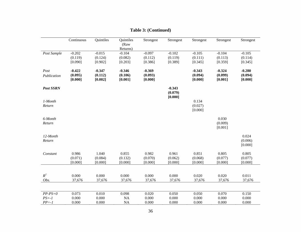
Table 3 presents regression estimates of how predictability varies through the life-cycle of

a publication. The first column, labeled “Continuous,” uses Fama-MacBeth coefficients (again,

scaled by in-sample means) generated from regressions that use continuous measures of the

characteristic (e.g., size or past returns) as the dependent variable. The results suggest that

between the end of the sample and the publication date, the magnitude of the long-short returns

fall, on average, by about 20%. We are unable to reject the hypothesis that this drop is

statistically significant from zero. Post-publication, the decline is 42% and statistically

significant from both 0 and -100%. Thus, cross-sectional predictability continues post-

publication at a significant, albeit muted level.

In the third column the dependent variable is the extreme quintiles return, not scaled by the

in-sample mean. The intercept in this regression is 0.855 (p-value = 0.000), thus the average in-

sample long-short return of the 72 anomalies is 85.5 basis points per month. The post-publication

coefficient is -0.346 and statistically significant, reflecting an average decline of 34.6 basis

points per month post-publication. The out-of-sample coefficient is -0.104, but not significant.

The fourth column returns to the scaled variables and uses either the Fama-MacBeth

coefficients from regressions that use continuous variables, or long-short extreme quintile

portfolios, depending on which method produces the highest in-sample statistical significance. In

this regression the post-publication decline is estimated to be 37%, which is similar to the slopes

(42% and 35%) estimated in the regressions that use the continuous and quintiles estimates

 

15  

respectively. If the original cross-sectional relations were purely noise, then selecting a

weighting method based on in-sample significance would produce the largest decay in post-

sample returns, however this is not the case.

The fourth column considers an alternative publication date that is based on either the

actual publication date or the first SSRN posting date, whichever is earlier. In this regression, the

post-publication coefficient estimates a decay of 34%, showing that small changes to publication

dates do not have an effect on the findings. This finding makes sense, since the post-publication

coefficient is essentially a test of the difference between the in-sample and post-publication

values of the normalized portfolio returns. We have a total of 9,984 post-publication portfolio-

month returns, which increases to 10,797 if we instead use the SSRN posting date as the

publication date. Hence, this change in definition increases the post-publication sample by only

7.5%, which is not a large difference.

Recent work by Moskowitz, Ooi, and Pedersen (2010) and Asness, Moskowitz and

Pedersen (2009) finds broad momentum across asset classes, and correlation of momentum

returns across classes. The pervasiveness of the results in these papers suggest that momentum,

or perhaps shorter-term persistence, might exist among our larger sample of characteristics. We

therefore include the portfolio’s last month’s return, the sum of the portfolio’s last 6 months’

returns, and the sum of the portfolio’s last 12 months’ returns in the final three regressions. All

three of these lagged return coefficients are positive and significant. These results show that

characteristic returns are persistent, which is broadly consistent with the findings of Moskowitz

et al. The publication coefficient remain significant each of these regressions, suggesting a post-

publication decline of about 30% once past returns are considered.

 

16  

At the bottom of Table 3, we report tests of whether the coefficient for post-publication is

greater than the coefficient for out-of-sample but pre-publication. In all but the last regressions

the difference is statistically significant. Hence, the decline in return-predictability that is

observed post-publication exceeds the decline in return-predictability that is observed out-of-

sample, but pre-publication. This difference tells us that there is an effect associated with

publication that cannot be explained by statistical biases, which should be fully reflected in the

out-of-sample but pre-publication coefficients.

3.3. Publication Effect or Time Trend?

It could be the case that the dissemination of academic research has no effect on return-

predictability, and that our end-of-sample and publication coefficients reflect a time trend, or a

trend that proxies for lower costs of corrective trading. As an example, it could be that anomalies

reflect mispricing, and declining trading costs have made arbitrage more effective, which is why

we observe the drop post-publication. Goldstein, Irvine, Kandel, and Wiener (2009) present

evidence that brokerage commissions dropped dramatically from 1977 to 2004, while Anand,

Irvine, Puckett and Venkataraman (2012) show that, over the last decade, execution costs have

fallen. Chorida, Subrahmanyam, and Tong (2011) show that in the 1993 to 1999 time period, ten

characteristics that were previously associated with cross-sectional returns failed to achieve

statistical significance. They attribute this result to lower transaction costs and more trading

activity from informed traders. Hence, it could be the case that characteristics are diminishing

because the costs of trading on these characteristics have declined over time.

We examine time series effects with four different time series variables. First, we construct

a time variable that is equal to 1/100 in January 1926 and increases by 1/100 during each

 

17  

consecutive month in our sample. Thus, a unit change in this variable corresponds to 8.33 years.

If transactions costs have been decreasing linearly over time, this variable should be negatively

associated with characteristic returns. Our second variable is a characteristic-specific time

variable that is equal to 1/100 during the first month after publication and increases by 1/100 in

each subsequent month. If sophisticated traders learn about characteristics slowly and linearly

after publication, then this should share a negative relation with characteristic returns. The

coefficients and standard errors for both of these monthly-time variables are reported in percent.

Third we use a post-1993 indicator variable to proxy for the discrete bifurcation of the data that

Chordia et al. use. Our final variable is an estimate of the average bid-ask spread as a percentage

of share price. The average is calculated using all the stocks that are traded in the CRSP universe

during the month. Spreads are estimated from daily high and low prices using the method of

Corwin and Schultz (2012).

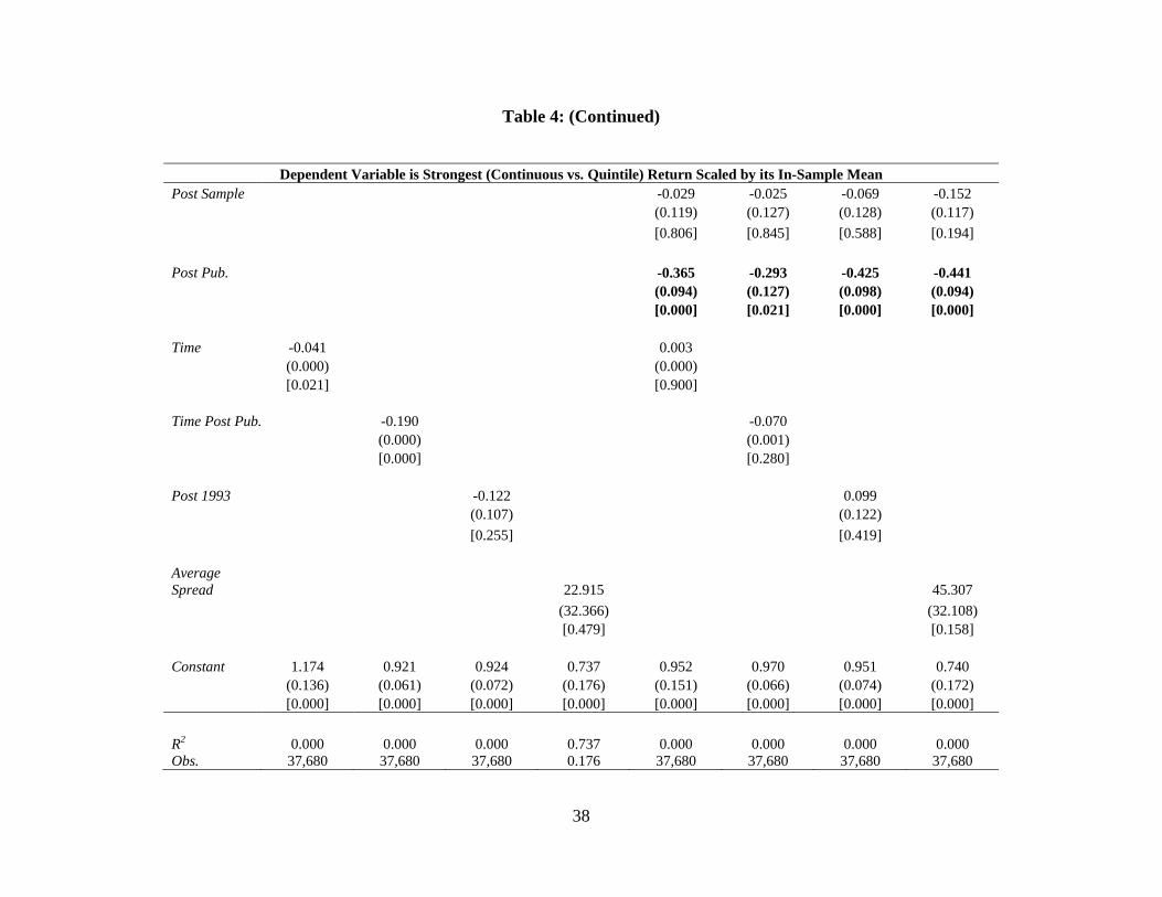
The regressions in Table 4 use the returns for the method (continuous vs. quintiles) that

produces the most statistically significant in-sample returns. In regressions where the time

variables are used without other regressors (columns 1-4), both months after 1926 (time) and

months after publication have negative slope coefficients that are significant at the 1% level. The

post 1993 indicator variable is -12.2%, which is consistent with Chordia et al., however the p-

value is 0.255, exceeding the typical bound of significance. The spreads coefficient is positive,

but not significant.

Columns 5-8 include both the time-series variables, and the post-sample and post-

publication indicators. As in Table 3, the slope of the post-sample indicator is negative and

insignificant for all specifications, while the slope on the post-publication indicator is negative

and significant in all of the regressions. The magnitude of the post-publication slope ranges from

 

18  

about -29% to -43%, similar to what is reported in Table 3. All of the time-series variables are

insignificant. Thus, this evidence implies that post-publication changes in predictability dominate

trends in predictability, which is insignificant in the presence of the post-publication indicator.

3.3. A Closer Look at Characteristic Dynamics

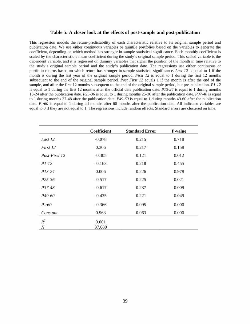
Table 5 further considers changes in predictability by examining finer post-sample and

post-publication partitions. This provides insight into whether authors or journals engage in

blatant data mining and whether the Table 4 specification is well-specified.

The regression contains dummy variables that signify the last 12 months of the original

sample; the first 12 months out-of sample; and the other out-of-sample months. In addition, the

publication dummy is split up into six different variables; one dummy for each of the first five

years post-publication, and one dummy for all of the months that are at least five years after

publication.

The publication process often takes years. This gives researchers the opportunity to

choose where to end their samples with the purpose of getting stronger results. In Table 5, the

coefficient for the last 12 months of the sample period is negative and insignificant, while the

coefficient for the first 12 months out-of-sample is positive and insignificant. The slopes on these

coefficients are the opposite signs to what we would expect if authors were opportunistically

select sample end dates.

The out of sample but pre-publication coefficient and the coefficients for the first 2 years

out of sample are all negative and similar in magnitude (-0.178 to -0.292), while the coefficients

for post-publication years 3, 4, and 5 demonstrate the biggest decay in predictability. For this

time period, predictability is about half of what it is in-sample. The coefficient for all months

 

19  

after the fifth year is -0.307. Hence, characteristics appear to make large declines during years 3-

5, and then partially recover thereafter, albeit still at a lower level than in-sample.

In untabulated results, we segment our sample of characteristics into categories of more

and less persistence. We measure persistence as average monthly portfolio turnover. For more

persistent characteristics, we expect the returns right after publication to be higher, since if new

capital flows to a strategy that is persistent, the characteristic stocks will be subject to

contemporaneous buying and selling pressure that exacerbate cross-sectional predictability in the

short run. Consistent with this idea, we find that less persistent strategies have a 78% larger

decay in the year following publication. Despite the large economic magnitude of this

coefficient, the statistical significance is marginal, in that null of equality at rejected at the 15.2%

level.

3.4. Publication and Trading in Characteristic Portfolios

If academic publication provides market participants with information that they trade on,

then this trading activity is likely to affect not only prices, but also other indicators of trading

activity. To test for such effects we perform monthly ranks based on turnover, dollar value of

trading volume, and stock return variance. Turnover is measured as shares traded scaled by

shares outstanding, while dollar volume is measured as shares traded multiplied by price.

Variance is calculated from monthly stock returns over the preceding thirty-six months. We

focus on rankings because these trading activity measures are likely to have market-wide time-

trends (e.g, turnover is, on average, higher now as compared to 1930). For each characteristic

portfolio, we compute the average ranking among the stocks that enter either the long or the

short side of the characteristic portfolio each month. We scale each portfolio-month ranking by

 

20  

the portfolio’s its in-sample average and test whether the ranking changes out-of-sample and

post-publication.

We also test whether relative shorting increases after a paper is published. We measure

short interest as shares shorted scaled by shares outstanding. Each month, we subtract the

average short interest of the long side of each characteristic-portfolio from the average short

interest of the short side of each characteristic portfolio. The long and short sides are the extreme

quintiles based on monthly sorts of each characteristics.

We report the results from these tests in Tables 6. Similar to Table 3, Table 6 estimates a

regression akin to Eq. (1); only the dependent variable is either the normalized rank of the

trading characteristic, or the difference between extreme quintiles in short interest, rather than

the normalized return. We cluster our standard errors on characteristic, rather than time, as the

traits tend to be persistent. Clustering on time in these regressions produces larger t-statistics.

The results show that variance and dollar volume are significantly higher during the period

that is post sample but pre-publication, while turnover is not. Hence, there appears to be an

increase in trading among characteristic stocks even before a paper is published, suggesting that

information from papers may get to some investors before the paper is published. The effects are

greatest with dollar volume; the average dollar volume rank of a firm in a characteristic portfolio

is 2.5% higher out-of-sample but pre-publication as compared to in-sample.

The slopes for variance, turnover, and dollar volume are all significantly higher post-

publication. Moreover each of the post-publication coefficients is greater than the out-of-sample

coefficient, although the differences are not statistically significant. The coefficients suggest that

post-publication, the average rank within the characteristic portfolios increases by 1.2%, 2.5%,

and 3.1% for variance, turnover, and dollar volume respectively.

 

21  

The final column reports the results from the short interest regression. Recall that the short

interest variable is the short interest on the short side minus the short interest on the long side.

This variable is not scaled by its in-sample mean, so the intercept reflects any difference in

shorting before the paper was published. The coefficients in this regression are reported in

percent. If investors recognize that characteristic stocks are mispriced, then there should be more

shorting on the short side than on the long side. The intercept is 0.109 (p-value =0.045), so the

average difference in short interest between the short and long side of the characteristic

portfolios was 0.109%, before publication. The mean and median levels of short interest in our

sample (1976-2011) are 3.45% and 0.77% respectively, so this difference is economically

meaningful. This result suggests that some practitioners knew that stocks in the characteristic

portfolios were mispriced, and traded accordingly. This could be because practitioners were

trading on the characteristic, or it could reflect practitioners trading on other strategies, which

happen to be correlated with the characteristics. As an example, short sellers might evaluate

firms individually with fundamental analyses. The resulting positions might be stocks with low

book-to-market ratios, high accruals, high stock returns over the last few years, etc., even though

short sellers were not directly choosing stocks on these traits.

Post-sample, relative shorting increases by 0.372, although the effect is not statistically

significant. Post-publication relative shorting increases by 0.935% relative to in-sample, and this

effect is statistically significant. Economically, the effect represents an increase in relative

shorting of nine-fold post-publication relative to in-sample. So although some practitioners may

have known about these strategies before publication, the results here suggest that publication

made the effects more widely known.

 

22  

3.5. Which Characteristics Decline the Most?

In this section we ask which characteristics decline the most post publication. Some of

the results in the previous tables are consistent with the idea that publication attracts arbitrageurs,

which results in smaller characteristic returns post-publication. As we explain in the

Introduction, Pontiff (1996, 2006) and Shleifer and Vishny (1997) point out that costs associated

with arbitrage can prevent arbitrageurs from fully eliminating mispricing. By this logic,

characteristic portfolios that consist more of stocks that are costlier to arbitrage (e.g., smaller

stocks, less liquid stocks, stocks with more idiosyncratic risk) should decline less post-

publication. If anomalous returns are the outcome of rational asset pricing, we would not expect

the post-publication decline to be related to arbitrage costs. Keep in mind that our returns are

scaled by the in-sample mean, so a decline implies that the returns shrink towards zero;

characteristics that produce negative returns have an increase in returns, while characteristics that

produce positive returns experience a decrease in returns.

Previous papers in the limited arbitrage literature relate arbitrage costs to differences in

returns across stocks within a characteristic portfolio (see Pontiff, 2006; Duan, Hu, and McLean,

2010; and McLean, 2010). In contrast, we estimate differences across characteristic portfolios.

Another difference between our test and previous literature is that previous studies assume

rational expectations of the informed traders through-out the entire sample. In this framework,

the informed trader had knowledge of the characteristic before (and after) the publication date.

Our current test assumes that publication provides information to some sophisticated traders,

which, in turn, causes decay in return-predictability post-publication.

To create the costly arbitrage variables, we perform monthly ranks of all of the stocks in

CRSP based on three transaction cost measures; size, dollar volume, and bid-ask spreads, and

 

23  

two holding costs measures: idiosyncratic risk and a dividend-payer dummy. Idiosyncratic risk is

a holding cost since idiosyncratic risk is incurred every period the position is open (Pontiff 1996

and 2006). We compute monthly idiosyncratic risk by regressing daily returns on the twelve

value-weighted industry portfolios from Ken French's website. For each day, we square that

day's residuals and, to correct for autocorrelation, add two times the product of that day's residual

and the previous day's residual. The monthly measure is created by adding up the daily data from

a given month.  

Pontiff (1996 and 2006) explains that dividends mitigate holding costs since they

decrease the effective duration of the position. We use a dummy variable equal to unity if a firm

paid a dividend and zero otherwise. Firm size is measured as the market value of equity. Average

monthly spreads are estimated from daily high and low prices using the method of Corwin and

Schultz (2012). Stocks with high dollar volume and low spreads are more liquid, and should

therefore be less costly to arbitrage.

For each characteristic-month, we compute the average ranking among the stocks that are

in either the long or the short side of the characteristic portfolio. We create a characteristic-

month average for each trait, and then take an average of the monthly averages to come up with a

single in-sample-characteristic average. We measure the traits in-sample, as it could be the case

that trading caused by publication has an effect on the variables.

We also consider other variables that we expect to be related to decay in predictability—

Sharpe ratio, t-statistic, and R2. The Sharpe ratio is a popular measure of portfolio performance

and we expect it to proxy for the attractiveness of the strategy to a professional trader, we

measure the Sharpe ratio by scaling each strategy’s in-sample mean monthly return by its in-

sample monthly return standard deviation. The t-statistic is simply the t-statistic that we compute

 

24  

for the in-sample portfolio return. We expect this variable to communicate the confidence of an

investor with respect to the predictability associated with the characteristic. R2 is a measure of

the systematic risk associated with characteristic. R2 is estimated in the regressions described in

section 1, in which we regress monthly stock returns on each trait (e.g., size, trading volume).

The R2 for each characteristic is the average R2 from the in-sample, monthly regressions. We

expect that characteristics that are associated with greater R2 are more likely to display

predictability that is the outcome of an asset pricing model, and thus, less likely to decay.  

In Table 7, the dependent variable is the normalized characteristic return, limited to post-

publication months. The results show that there are significantly larger post-publication declines

for characteristic portfolios with lower arbitrage costs. Characteristic portfolios that on average

consist of larger stocks, stocks with smaller bid ask spreads, and stocks with high dollar volume

decline more. Characteristic portfolios that on average consist of stocks with lower idiosyncratic

volatility and stocks that pay dividends also decline more post-publication. Sharpe ratios, t-

statistics, and systematic risk do not exhibit a significant relation to the decay in a characteristics

stock return-predictability.

3.6. Which Arbitrage Costs Matter Most?

In the previous section the results show that size, spreads, dollar volume, idiosyncratic

risk, and dividends all have statistically significant effects on a characteristic’s post-publication

decay. In this section we try to determine which of these variables has the greatest effect.

In Table 8, the first regression includes only dividends and idiosyncratic risk, and we see

that idiosyncratic risk makes the effect of dividends insignificant, while the idiosyncratic risk

coefficient is positive and significant, as it was in the previous table. In the next three regressions

 

25  

we add in each of the transaction cost variables, and find that each of these is insignificant in the

presence of idiosyncratic risk and dividends. Throughout all of the regressions in Table 8,

idiosyncratic risk is the only factor that has a significant effect on the post-publication decline.

This results is consistent with Pontiff (2006), who reviews a literature that relates arbitrage costs

to alpha across stocks within characteristic portfolios. This literature finds that characteristic

return-predictability stronger in stocks with high idiosyncratic risk, even more so than stocks

with high transaction costs.

3.7. The Effects of Publication on Correlations Access Characteristic Portfolios

In this section, we study the effects that publication has on the correlation across

characteristic portfolios. We consider whether or not publication affects correlation, and whether

or not months with poor characteristic-based returns are associated with higher correlations.

All long-short portfolios are constructed such that long leg has an in-sample mean return

that is higher than the short leg. Simple correlations between characteristic based portfolios are

lower than we expected. The mean pairwise correlation in our study is 0.050 and the median is

0.047. These levels of correlation imply even lower covariance than Green et al. (2012), who

show that R2 between characteristic returns ranges from 6% to 20%. Our results and the Green et

al. results suggest that multi-characteristic investing is likely to enjoy substantial diversification

benefits.

If characteristics reflect mispricing and if mispricing has common causes (e.g. investor

sentiment), then we might expect in-sample characteristic portfolios to be correlated with other

in-sample characteristic portfolios. This effect is shown in Lee, Shleifer, and Thaler (1991) and

Barberis and Shelifer (2003). If publication causes arbitrageurs to trade in a characteristic, then it

 

26  

could cause a characteristic portfolio to become more highly correlated with other published

characteristics and less correlated with unpublished characteristics.

In Table 9, each characteristic portfolio’s return is regressed on an equal-weighted

portfolio of all of the other characteristics that are pre-publication and an equal-weighted

portfolio of all of the other characteristics that are post-publication. We include a dummy

variable that indicates whether the characteristic is post-publication, and interactions between

this dummy variable and the pre-publication and post-publication characteristic portfolios

returns. As before, the monthly characteristic returns are scaled by their in-sample mean.

The results show that while a characteristic is pre-publication, the associated

characteristic portfolio returns are significantly related to the returns of other pre-publication

characteristic portfolios. The slope coefficient is 0.634 and its p-value is 0.00. In contrast, the

slope coefficient or beta of a pre-publication portfolio with portfolios that are post-publication is

0.025. These findings are consistent with Lee, Shleifer, and Thaler (1991) and Barberis and

Shleifer (2003).

The interactions show that once a characteristic is published, the returns on its respective

portfolio is less correlated with the returns of other pre-publication characteristic portfolios, and

more correlated with the returns of other post-publication characteristic portfolios. The slope on

the interaction of the post-publication dummy with the return of the portfolio consisting of in-

sample characteristics is -0.555 (p-value = 0.00). Hence, once a characteristic is published, the

correlation of its returns with the returns of other yet-to-be-published characteristic returns

virtually disappears, as the overall coefficient reduces to 0.634 – 0.555 = 0.079. The slope on the

interaction of the post-publication dummy and the returns of the other post-publication

 

27  

characteristics is 0.399 (p-value = 0.00), so there is a significant correlation between the portfolio

returns of a published characteristic and other published characteristics.

4. Conclusions

This paper studies 82 characteristics that have been shown to explain cross-sectional

stock returns in peer reviewed finance, accounting, and economics journals. We compare each

characteristic’s return predictability over three distinct periods: (i) within the original study’s

sample period; (ii) outside of the original sample period but before publication; and (iii) post

publication.

We use the period during which a characteristic is outside of its original sample but still

pre-publication to estimate an upper bound on the effect of statistical biases. We estimate the

effect of statistical bias to be about 10%. The average characteristic’s return decays by about

35% post-publication. We attribute this post-publication effect both to statistical biases, and to

arbitrageurs who observe the finding. Combining this finding with an estimated statistical bias of

10% implies a lower bound on the publication effect of about 25%.

Our findings support the contention that cross-sectional predictability is the result of

mispricing. Academic research draws attention to characteristic strategies, which results in more

trading in characteristic-portfolio stocks. First, variance, turnover, dollar volume, and short

interest all increase significantly in characteristic portfolios post-publication. Second,

characteristic portfolios that consist more of stocks that are costly to arbitrage decline less post-

publication. This is consistent with the idea that arbitrage costs limit arbitrage and protect

mispricing. Finally, we find that before a characteristic is featured in an academic publication,

the returns of the corresponding characteristic portfolio are highly correlated to the returns of

 

28  

other portfolios of yet-to-be-published characteristic stocks. This is consistent with behavioral

finance models of comovement. After publication, the sensitivity to yet-to-be-published

characteristic portfolios returns decreases and the sensitivity to already-published characteristic

portfolios returns increases.

 

29  

References

Ang, Andrew, Robert J. Hodrick, Yuhang Xing, and Xiaoyan Zhang, 2006, “The cross-section of volatility and expected returns,” Journal of Finance 61, 259-299.

Amihud, Yakov, 2002, “Illiquidity and stock returns: Cross-section and time-series effects,”

Journal of Financial Markets 5, 31-56. Amihud, Yakov, and Haim Mendelson, 1986, “Asset pricing and the bid–ask spread,” Journal of

Financial Economics 17, 223–249. Anand, Amber, Paul Irvine, Andy Puckett, and Kumar Venkataraman, forthcoming,

“Performance of Institutional Trading Desks: An Analysis of Persistence in Trading Costs,” Review of Financial Studies.

Asness, Clifford S., Tobias J. Moskowitz, and Lasse H. Pedersen, 2009, “Value and momentum

everywhere,” Working paper, New York University. Barberis, Nicholas, and Andrei Shleifer, 2003, “Style investing,” Journal of Financial

Economics 68, 161-199. Bali, Turan G., and Nusret Cakici, 2008, “Idiosyncratic Volatility and the Cross Section of

Expected Returns,” Journal of Financial and Quantitative Analysis 43, 29-58. Bali, Turan G., Nusret Cakici, and F. Robert Whitelaw, 2011, “Maxing out: Stocks as lotteries

and the cross-section of expected returns,” Journal of Financial Economics 99, 427-446. Banz, Rolf W., 1981, “The relationship between return and market value of common stocks,”

Journal of Financial Economics 9, 3-18. Barberis, Nicholas, Andrei Shleifer, and Jeffrey Wurgler, 2005, “Comovement,” Journal of

Financial Economics 75, 283-317. Blume, Marshal E. and Frank, Husic, 1973, “Price, beta, and exchange listing,” Journal of

Finance 28, 283-299. Boyer, Brian, 2011, "Style-related Comovement: Fundamentals or Labels?," Journal of Finance

66, 307-332. Brennan, Michael J., 1970, “Taxes, market valuation, and corporate financial policy,” National

Tax Journal 23, 417–427. Chorida, Tarun, Avanidhar Subrahmanyam, and Qing Tong, 2011, “Trends in the cross-section

of expected stock returns,” Working paper, Emory University. Cochrane, John H., 1999, “Portfolio Advice for a Multifactor World,” Economic Perspectives

Federal Reserve Bank of Chicago 23, 59-78.

 

30  

Corwin, Shane A., and Paul Schultz, 2012, “A Simple Way to Estimate Bid-Ask Spreads from

Daily High and Low Prices,” Journal of Finance 67, 719-759.  

Duan, Ying, Gang Hu, and R. David McLean, 2009, “When is Stock-Picking Likely to be Successful? Evidence from Mutual Funds,” Financial Analysts Journal 65, 55-65.

Duan, Ying, Gang Hu, and R. David McLean, 2009, “Costly Arbitrage and Idiosyncratic Risk:

Evidence from Short Sellers,” Journal of Financial Intermediation 19, 564-579. De Long, J.B., Shleifer, A., Summers, L.H., Waldmann, R.J., 1990, “Noise trader risk in

financial markets,” Journal of Political Economy 98, 703–738. Dichev, Ilia D., 1998, “Is the Risk of Bankruptcy a Systematic Risk?,” The Journal of Finance

53, 1131-1148. Dichev, Ilia D., and Joseph D. Piotroski, 2001, “The long-run stock returns following bond

ratings changes,” Journal of Finance 56, 173-203. Fama, Eugene F., 1976, Foundations of Finance, Basic Books, New York (New York). Fama, Eugene F., 1991, “Efficient capital markets: II,” Journal of Finance 46, 1575-1617. Fama, Eugene F., and French, Kenneth R., 1992, “The cross-section of expected stock returns,”

Journal of Finance 47, 427-465. Fama, Eugene F., and James D. MacBeth, 1973, “Risk, return, and equilibrium: Empirical tests,”

Journal of Political Economy 81, 607-636. Franzoni, Francesco and Jose M. Marin, 2006, “Pension Plan Funding and Stock Market

Efficiency,” Journal of Finance 61, 921-956. Greenwood, Robin. 2008, "Excess Comovement of Stock Returns: Evidence from Cross-

sectional Variation in Nikkei 225 Weights," Review of Financial Studies 21, 1153-1186. Goldstein, Michael, Paul Irvine, Eugene Kandel, and Zvi Weiner, 2009, “Brokerage

commissions and Institutional trading patterns,” Review of Financial Studies 22, 5175-5212 Hanson, Samuel G., and Adi Sunderam, 2011, “The growth and limits of arbitrage: Evidence

from short interest,” Working paper, Harvard Business School. Haugen, Robert A, and Nardin L. Baker, 1996, “Commonality in the determinants of expected

stock returns,” Journal of Financial Economics 41, 401-439. Heckman, James, 1979, "Sample selection bias as a specification error," Econometrica 47, 153–

161.

 

31  

Hedges, Larry V., 1992, “Modeling publication selection effects in meta-analysis,” Statistical

Science 7, 246-255. Hwang, Byoung-Hyoun and Baixiao Liu, 2012, “Which anomalies are more popular? And

Why?, Purdue working paper. Goyal, Amit, and Ivo Welch, 2008, “A comprehensive look at the empirical performance of

equity premium prediction,” Review of Financial Studies 21, 1455-1508. Green, Jeremiah, John R. M. Hand, and X. Frank Zhang, 2012, “The Supraview of Return

Predictive Signals,” Working paper, Pennsylvania State University. Grundy, Bruce D. and Spencer J. Martin, J. Spencer, 2001, "Understanding the Nature of the

Risks and the Source of the Rewards to Momentum Investing," Review of Financial Studies 14, 29-78.

Jegadeesh, Narasimhan and Sheridan Titman, 1993, “Returns to Buying Winners and Selling

Losers: Implications for Stock Market Efficiency,” Journal of Finance 48, 65-91. Jegadeesh, Narasimhan, and Sheridan Titman, 2001, “Profitability of momentum strategies: An

evaluation of alternative explanations,” Journal of Finance 56, 699-720. Jegadeesh, Narasimhan and Sheridan Titman, 2011, “Momentum,” Working paper, Emory

University. LeBaron, Blake, 2000, “The Stability of Moving Average Technical Trading Rules on the Dow

Jones Index,” Derivatives Use, Trading and Regulation 5, 324-338. Leamer, Edward E., 1978, Specification Searches: Ad Hoc Inference with Nonexperimental

Data, New York: John Wiley & Sons. Lee, Charles, Andrei Shleifer, and Richard Thaler, 1991, Investor sentiment and the closed-end

fund puzzle, Journal of Finance 46, 75-109. Lewellen, Johnathan, 2011, “The cross-section of expected returns,” Working paper, Tuck

School of Business, Dartmouth College. Lo, Andrew, and Craig MacKinlay, 1990, “Data-snooping biases in tests of financial asset

pricing models,” Review of Financial Studies 3, 431-467. McLean, R. David, 2010, “Idiosyncratic risk, long-term reversal, and momentum,” Journal of

Financial and Quantitative Analysis, 45, 883-906. Michaely, Roni, Richard Thaler, and Kent L. Womack, 1995, “Price reactions to dividend

initiations and omissions: Overreaction or drift?,” Journal of Finance 50, 573-608.

 

32  

Mittoo, Usha, and Rex Thompson, 1990, “Do capital markets learn from financial economists?,”

working paper, Southern Methodist University Moskowitz, Tobias, Yao Hua Ooi, and Lasse H. Pedersen, 2010, “Time series momentum,”

Working paper, New York University. Muth, John F., 1961, “Rational Expectations and the Theory of Price Movements,”

Econometrica 29, 315–335. Naranjo, Andy, M. Nimalendran, and Mike Ryngaert, 1998, “Stock returns, dividend yields and

taxes,” Journal of Finance 53, 2029-2057. Pontiff, Jeffrey, 1996, “Costly arbitrage: Evidence from closed-end funds,” Quarterly Journal of

Economics 111, 1135-1151. Pontiff, Jeffrey, 2006, “Costly arbitrage and the myth of idiosyncratic risk,” Journal of

Accounting and Economics 42, 35-52. Ritter, Jay R., 1991, “The long-run performance of initial public offerings,” Journal of Finance

46, 3-27. Schwert, G. William, 2003, “Anomalies and market efficiency,” Handbook of the Economics of

Finance, edited by G.M. Constantinides, M. Harris and R. Stulz, Elsevier Science B.V. Sharpe, William F., 1964, “Capital asset prices: A theory of market equilibrium under conditions

of risk,” Journal of Finance 19, 425-442 Shleifer, Andrei, and Robert W. Vishny, 1992, “Liquidation Values and Debt Capacity: A

Market Equilibrium Approach,” Journal of Finance 47, 1343-1366 Sloan, Richard G., 1996, “Do stock prices fully reflect information in accruals and cash flows

about future earnings?,” Accounting Review 71, 289-315 Stein, Jeremy C, 2009, “Presidential address: Sophisticated investors and market efficiency,”

Journal of Finance 64, 1517-1548. Sullivan, Ryan, Allan Timmermann, and Halbert White, 2001, Dangers of data mining: The cse

of calendar effects in stock returns, Journal of Econometrics 105, 249-286. Treynor, Jack, and Fischer Black, 1973, How to Use Security Analysis to Improve Portfolio

Selection,” Journal of Business 46, 66-86. Wahal, Sunil, and M. Deniz Yavuz, 2009, “Style Investing, Comovement and Return

Predictability,” Working Paper, Arizona State University.

 

33  

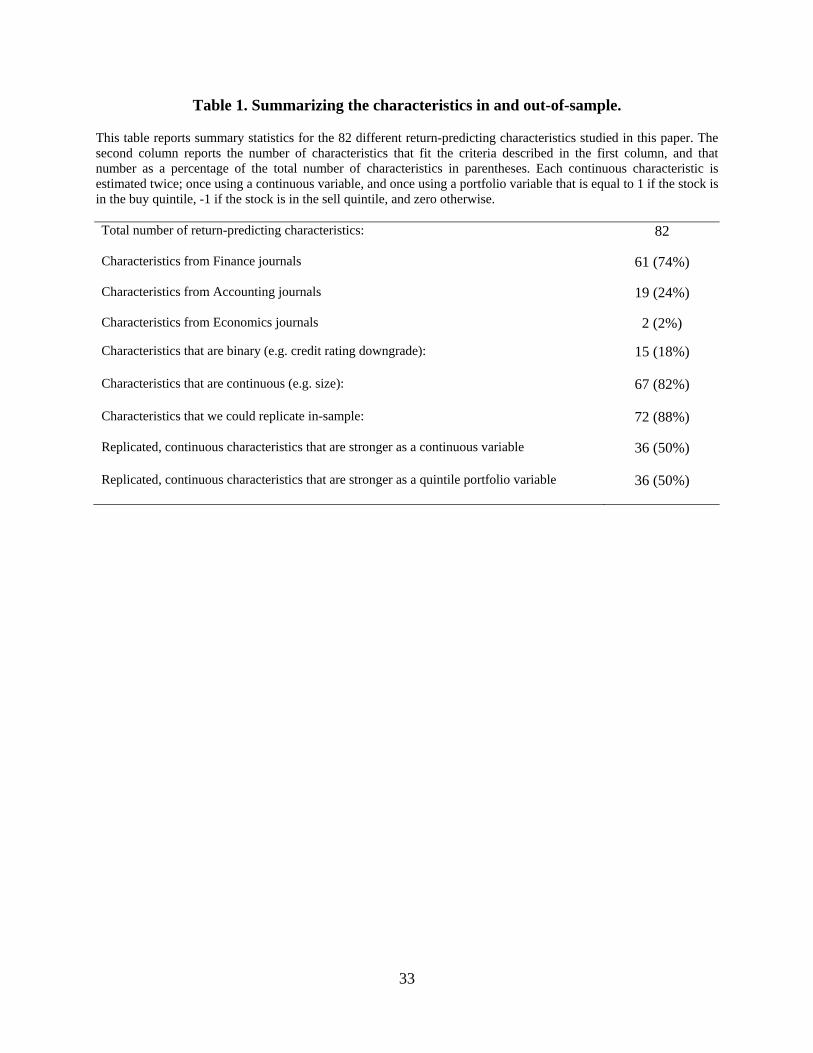
Table 1. Summarizing the characteristics in and out-of-sample.

This table reports summary statistics for the 82 different return-predicting characteristics studied in this paper. The second column reports the number of characteristics that fit the criteria described in the first column, and that number as a percentage of the total number of characteristics in parentheses. Each continuous characteristic is estimated twice; once using a continuous variable, and once using a portfolio variable that is equal to 1 if the stock is in the buy quintile, -1 if the stock is in the sell quintile, and zero otherwise. Total number of return-predicting characteristics: 82

Characteristics from Finance journals

61 (74%)

Characteristics from Accounting journals

19 (24%)

Characteristics from Economics journals 2 (2%)

Characteristics that are binary (e.g. credit rating downgrade): 15 (18%)

Characteristics that are continuous (e.g. size): 67 (82%)

Characteristics that we could replicate in-sample: 72 (88%)

Replicated, continuous characteristics that are stronger as a continuous variable 36 (50%)

Replicated, continuous characteristics that are stronger as a quintile portfolio variable 36 (50%)

 

34  

Table 2. Summarizing the out-of-sample and post-publication return predictability of the characteristics.

This table reports summary statistics for the out-of-sample and post-publication return predictability of the 82 replicated return-predicting characteristics used in this paper. To be included in these tests the characteristic had to both be replicated in-sample, and have at least 36 observations in the out-of-sample or post-publication measurement period. Each continuous characteristic is estimated twice, first using a continuous variable, and then using a portfolio variable that is equal to 1 if the stock is in the long quintile, -1 if the stock is in the sell quintile, and zero otherwise. We estimate the in-sample mean coefficient for each characteristic, and then scale each monthly coefficient by the in-sample mean. We then take averages of the scaled coefficients during the out-of-sample and post-publication periods for each characteristic, average the averages across characteristics, and report these statistics in the table below. A value of 1 means the average characteristic-portfolio is the same during the in-sample and out-of-sample period. A value of less than 1 (greater than 1) means the return-predictability declined (increased) out-of-sample. The t-statistic tests whether the reported value is equal to 1.

 

Panel A: Continuous

Out of Sample but Pre-

Publication Post Publication

Average Scaled Coefficient 0.78 0.51

Standard Deviation 1.22 0.81

t-statistic -1.40 -4.91

Percentage <1 63% 82%

Anomalies Included 60 66

Panel B: Quintile

Out of Sample but Pre-

Publication Post Publication

Average Scaled Coefficient 0.90 0.47

Standard Deviation 1.29 1.20

t-statistic -0.58 -3.62

Percentage <1 57% 68%

Anomalies Included 60 66

Panel C: Strongest

Out of Sample but Pre-

Publication Post Publication

Average Scaled Coefficient 0.77 0.51

Standard Deviation 1.16 0.97

t-statistic -1.56 -4.02

Percentage <1 65% 78%

Anomalies Included 60 66

 

35  

Table 3. Regression of long-short characteristic based returns on time indicator variables.

This regression models the return-predictability of each characteristic over time, relative to its original sample period and publication date. Each monthly coefficient is scaled by the characteristic’s mean coefficient during the study’s original sample period. This scaled variable is the dependent variable, and it is regressed on dummy variables that signal whether the month is out of sample but pre-publication, and post-publication. Post Sample equals 1 if the month is after the end of the sample, but pre-publication. Post Publication is equal to 1 if the month is after the official publication date. Post SSRN is equal to 1 if the month is either after the official publication date, or if the month is after the first month that the study is available on SSRN. All indicator variables are equal to 0 if they are not equal to 1. We also include lagged values measured over the last 1 month, and the sum of returns over the last 6 and 12 months. The regression labeled Continuous uses Fama-MacBeth slopes that are generated using continuous variables. The regression labeled Quintiles uses Fama-MacBeth slopes from long-short quintile portfolios. The regression labeled Strongest uses either Continuous or Quintiles returns, depending on which method produces stronger in-sample statistical significance. P-values are in brackets for the hypothesis that the coefficient equals 0. In the three bottom rows we report p-values from Chi-Squared tests of the hypotheses that the post-sample and post-publication coefficients are equal, and that each of the coefficients is equal to -1. The regressions include random effects. Standard errors are clustered on time.

 

36  

Table 3: (Continued)

Continuous Quintiles Quintiles (Raw

Returns)

Strongest Strongest Strongest Strongest Strongest

Post Sample -0.202 (0.119) [0.090]

-0.015 (0.124) [0.902]

-0.104 (0.082) [0.203]

-0.097 (0.112) [0.386]

-0.102 (0.119) [0.389]

-0.105 (0.111) [0.345]

-0.104 (0.113) [0.359]

-0.105 (0.114) [0.345]

Post Publication

-0.422 (0.095) [0.000]

-0.347 (0.112) [0.002]

-0.346 (0.106) [0.001]

-0.369 (0.093) [0.000]

-0.343 (0.094) [0.000]

-0.324 (0.099) [0.001]

-0.280 (0.094) [0.000]

Post SSRN -0.343 (0.079) [0.000]

1-Month Return

0.134 (0.027) [0.000]

6-Month Return

0.030 (0.009) [0.001]

12-Month Return

0.024 (0.006) [0.000]

Constant 0.986

(0.071) [0.000]

1.040 (0.084) [0.000]

0.855 (0.132) [0.000]

0.982 (0.070) [0.000]

0.961 (0.062) [0.000]

0.851 (0.068) [0.000]

0.805 (0.077) [0.000]

0.805 (0.077) [0.000]

R2 0.000 0.000 0.000 0.000 0.000 0.020 0.020 0.011 Obs. 37,676 37,676 37,676 37,676 37,676 37,676 37,676 37,676

PP-PS=0 0.073 0.010 0.098 0.020 0.050 0.050 0.070 0.150 PS=-1 PP=-1

0.000 0.000

0.000 0.000

NA NA

0.000 0.000

0.000 0.000

0.000 0.000

0.000 0.000

0.000 0.000

 

37  

Table 4: Time Trend vs. Publication Effect

This regression models the return-predictability of each characteristic over time, and relative to the characteristic’s original sample period and publication date. We use either continuous variables or quintile portfolios based on the variables to generate the coefficient, depending on which method has stronger in-sample statistical significance. Each monthly coefficient is scaled by the characteristic’s mean coefficient during the study’s original sample period. This scaled variable is the dependent variable, and it is regressed on dummy variables that signal whether the month is out of sample but pre-publication, and post-publication. Post Sample equals 1 if the month is after the end of the sample, but pre-publication. Post Publication is equal to 1 if the month is after the official date publication date. Time is the number of months (in hundreds) post-Jan. 1926. Time Post-Publication is the number of months (in hundreds) post-publication. The time coefficients and standard errors are reported in percent. Post-1993 is equal to1 if the year is greater than 1993 and 0 otherwise. All indicator variables are equal to 0 if they are not equal to 1. Average Spread is the average estimated bid-ask spread as a percentage of the share price of all CRSP stocks. Fama-MacBeth slopes from either continuous variables, or long-short extreme quintiles, are used based on which return has stronger in-sample statistical significance. P-values are in brackets for the hypothesis that the coefficient equals 0. In the three bottom rows, we report p-values from Chi-Squared tests of the hypotheses that the post-sample and post-publication coefficients are equal, and that each of the coefficients is equal to -1. The regressions include random effects. Standard errors are clustered on time.

 

38  

Table 4: (Continued)

Dependent Variable is Strongest (Continuous vs. Quintile) Return Scaled by its In-Sample Mean

Post Sample -0.029 -0.025 -0.069 -0.152 (0.119) (0.127) (0.128) (0.117) [0.806] [0.845] [0.588] [0.194]

Post Pub. -0.365 -0.293 -0.425 -0.441 (0.094) (0.127) (0.098) (0.094) [0.000] [0.021] [0.000] [0.000]

Time -0.041 0.003 (0.000) (0.000) [0.021] [0.900]

Time Post Pub. -0.190 -0.070 (0.000) (0.001)

[0.000] [0.280]

Post 1993 -0.122 0.099 (0.107) (0.122)

[0.255] [0.419]

Average Spread 22.915 45.307

(32.366) (32.108) [0.479] [0.158]

Constant 1.174 0.921 0.924 0.737 0.952 0.970 0.951 0.740

(0.136) (0.061) (0.072) (0.176) (0.151) (0.066) (0.074) (0.172) [0.000] [0.000] [0.000] [0.000] [0.000] [0.000] [0.000] [0.000]

R2 0.000 0.000 0.000 0.737 0.000 0.000 0.000 0.000 Obs. 37,680 37,680 37,680 0.176 37,680 37,680 37,680 37,680

 

39  

Table 5: A closer look at the effects of post-sample and post-publication

This regression models the return-predictability of each characteristic relative to its original sample period and publication date. We use either continuous variables or quintile portfolios based on the variables to generate the coefficient, depending on which method has stronger in-sample statistical significance. Each monthly coefficient is scaled by the characteristic’s mean coefficient during the study’s original sample period. This scaled variable is the dependent variable, and it is regressed on dummy variables that signal the position of the month in time relative to the study’s original sample period and the study’s publication date. The regressions use either continuous or portfolio returns based on which return has stronger in-sample statistical significance. Last 12 is equal to 1 if the month is during the last year of the original sample period. First 12 is equal to 1 during the first 12 months subsequent to the end of the original sample period. Post First 12 equals 1 if the month is after the end of the sample, and after the first 12 months subsequent to the end of the original sample period, but pre-publication. P1-12 is equal to 1 during the first 12 months after the official date publication date. P13-24 is equal to 1 during months 13-24 after the publication date. P25-36 is equal to 1 during months 25-36 after the publication date. P37-48 is equal to 1 during months 37-48 after the publication date. P49-60 is equal to 1 during months 49-60 after the publication date. P>60 is equal to 1 during all months after 60 months after the publication date. All indicator variables are equal to 0 if they are not equal to 1. The regressions include random effects. Standard errors are clustered on time.

Coefficient Standard Error P-value

Last 12 -0.078 0.215 0.718

First 12 0.306 0.217 0.158

Post-First 12 -0.305 0.121 0.012

P1-12 -0.163 0.218 0.455

P13-24 0.006 0.226 0.978

P25-36 -0.517 0.225 0.021

P37-48 -0.617 0.237 0.009

P49-60 -0.435 0.221 0.049

P>60 -0.366 0.095 0.000

Constant 0.963 0.063 0.000

R2 0.001 N 37,680

 

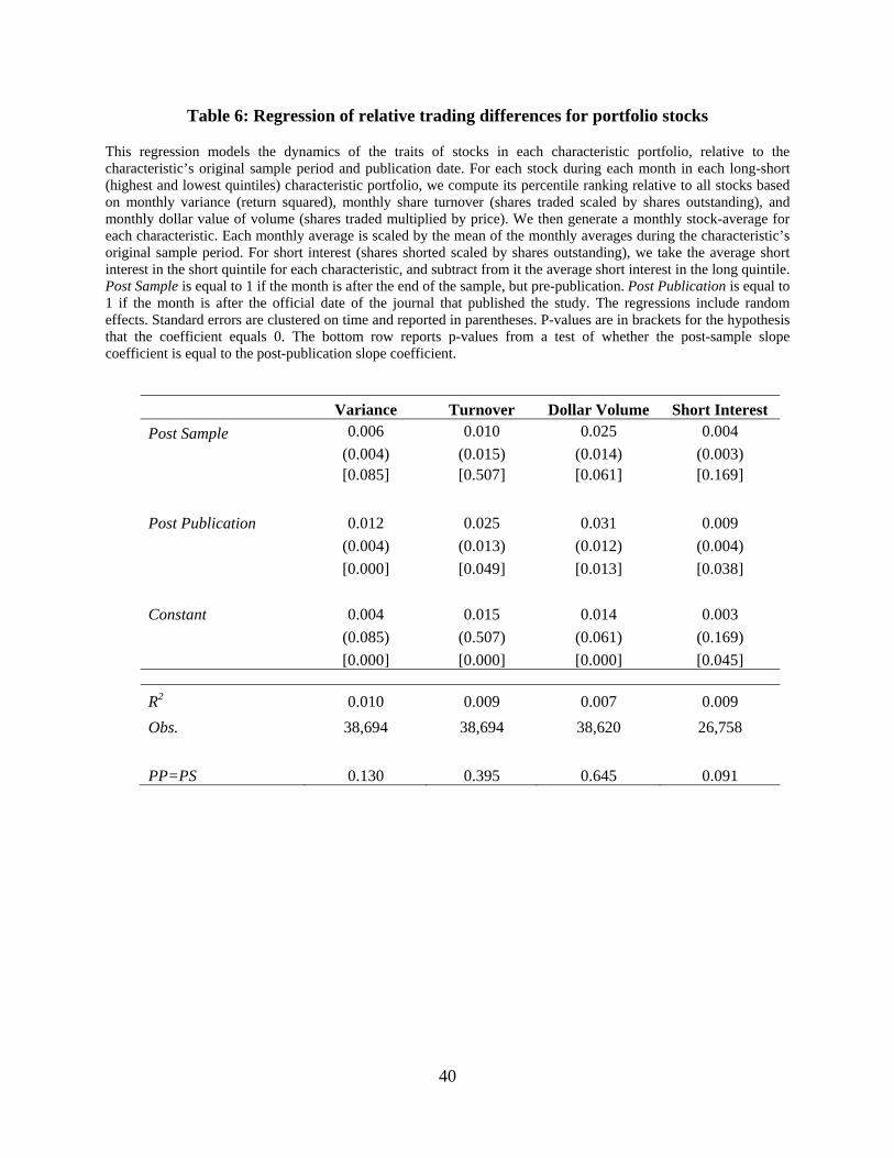
40  

Table 6: Regression of relative trading differences for portfolio stocks

This regression models the dynamics of the traits of stocks in each characteristic portfolio, relative to the characteristic’s original sample period and publication date. For each stock during each month in each long-short (highest and lowest quintiles) characteristic portfolio, we compute its percentile ranking relative to all stocks based on monthly variance (return squared), monthly share turnover (shares traded scaled by shares outstanding), and monthly dollar value of volume (shares traded multiplied by price). We then generate a monthly stock-average for each characteristic. Each monthly average is scaled by the mean of the monthly averages during the characteristic’s original sample period. For short interest (shares shorted scaled by shares outstanding), we take the average short interest in the short quintile for each characteristic, and subtract from it the average short interest in the long quintile. Post Sample is equal to 1 if the month is after the end of the sample, but pre-publication. Post Publication is equal to 1 if the month is after the official date of the journal that published the study. The regressions include random effects. Standard errors are clustered on time and reported in parentheses. P-values are in brackets for the hypothesis that the coefficient equals 0. The bottom row reports p-values from a test of whether the post-sample slope coefficient is equal to the post-publication slope coefficient.

Variance Turnover Dollar Volume Short Interest

Post Sample 0.006 0.010 0.025 0.004

(0.004) (0.015) (0.014) (0.003) [0.085] [0.507] [0.061] [0.169]

Post Publication 0.012 0.025 0.031 0.009

(0.004) (0.013) (0.012) (0.004)

[0.000] [0.049] [0.013] [0.038]

Constant 0.004 0.015 0.014 0.003

(0.085) (0.507) (0.061) (0.169)

[0.000] [0.000] [0.000] [0.045]

R2 0.010 0.009 0.007 0.009

Obs. 38,694 38,694 38,620 26,758

PP=PS 0.130 0.395 0.645 0.091

 

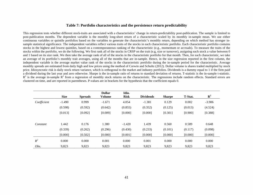
41  

Table 7: Portfolio characteristics and the persistence return predictability

This regression tests whether different stock-traits are associated with a characteristics’ change in return-predictability post-publication. The sample is limited to post-publication months. The dependent variable is the monthly long-short return of a characteristic scaled by its monthly in-sample mean. We use either continuous variables or quintile portfolios based on the variables to generate the characteristic’s monthly return, depending on which method has stronger in-sample statistical significance. The independent variables reflect various traits of the stocks in each characteristic portfolio. Each characteristic portfolio contains stocks in the highest and lowest quintiles, based on a contemporaneous ranking of the characteristic (e.g., momentum or accruals). To measure the traits of the stocks within the portfolio, we do the following. We first rank all of the stocks in CRSP on the trait (e.g, size or turnover), assigning each stock a value between 0 and 1 based on its size rank. We then take the average rank of all of the stocks in the characteristic portfolio for that month. Then, for each characteristic, we take an average of its portfolio’s monthly trait averages, using all of the months that are in-sample. Hence, in the size regression reported in the first column, the independent variable is the average market value rank of the stocks in the characteristic portfolio during the in-sample period for the characteristic. Average monthly spreads are estimated from daily high and low prices using the method of Corwin and Schultz (2012). Dollar volume is shares traded multiplied by stock price. Idiosyncratic risk is daily stock return variance, which is orthogonal to the market and industry portfolios. Dividends is a dummy equal to 1 if the firm paid a dividend during the last year and zero otherwise. Sharpe is the in-sample ratio of returns to standard deviation of returns. T-statistic is the in-sample t-statistic. R2 is the average in-sample R2 from a regression of monthly stock returns on the characteristic. The regressions include random effects. Standard errors are clustered on time, and are reported in parentheses. P-values are in brackets for the hypothesis that the coefficient equals 0.

Size Spreads Dollar

Volume Idio. Risk Dividends Sharpe T-Stat. R2

Coefficient -1.490 0.999 -1.671 4.054 -1.381 0.129 0.002 -3.906

(0.598) (0.592) (0.642) (0.855) (0.352) (0.125) (0.013) (4.524)

[0.013] [0.092] [0.009] [0.000] [0.000] [0.301] [0.900] [0.388]

Constant 1.442 0.176 1.380 -1.420 1.439 0.560 0.589 0.648

(0.339) (0.262) (0.296) (0.430) (0.233) (0.101) (0.117) (0.098)

[0.000] [0.502] [0.000] [0.001] [0.000] [0.000] [0.000] [0.000]

R2 0.000 0.000 0.001 0.000 0.001 0.000 0.000 0.000

Obs. 9,823 9,823 9,823 9,823 9,823 9,823 9,823 9,823

 

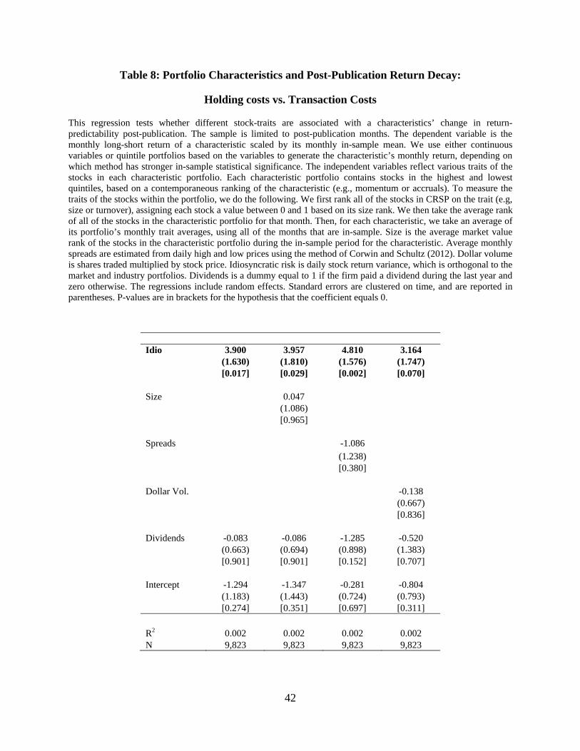
42  

Table 8: Portfolio Characteristics and Post-Publication Return Decay:

Holding costs vs. Transaction Costs

This regression tests whether different stock-traits are associated with a characteristics’ change in return-predictability post-publication. The sample is limited to post-publication months. The dependent variable is the monthly long-short return of a characteristic scaled by its monthly in-sample mean. We use either continuous variables or quintile portfolios based on the variables to generate the characteristic’s monthly return, depending on which method has stronger in-sample statistical significance. The independent variables reflect various traits of the stocks in each characteristic portfolio. Each characteristic portfolio contains stocks in the highest and lowest quintiles, based on a contemporaneous ranking of the characteristic (e.g., momentum or accruals). To measure the traits of the stocks within the portfolio, we do the following. We first rank all of the stocks in CRSP on the trait (e.g, size or turnover), assigning each stock a value between 0 and 1 based on its size rank. We then take the average rank of all of the stocks in the characteristic portfolio for that month. Then, for each characteristic, we take an average of its portfolio’s monthly trait averages, using all of the months that are in-sample. Size is the average market value rank of the stocks in the characteristic portfolio during the in-sample period for the characteristic. Average monthly spreads are estimated from daily high and low prices using the method of Corwin and Schultz (2012). Dollar volume is shares traded multiplied by stock price. Idiosyncratic risk is daily stock return variance, which is orthogonal to the market and industry portfolios. Dividends is a dummy equal to 1 if the firm paid a dividend during the last year and zero otherwise. The regressions include random effects. Standard errors are clustered on time, and are reported in parentheses. P-values are in brackets for the hypothesis that the coefficient equals 0.

Idio 3.900 3.957 4.810 3.164

(1.630) (1.810) (1.576) (1.747) [0.017] [0.029] [0.002] [0.070]

Size 0.047 (1.086) [0.965]

Spreads -1.086 (1.238) [0.380]

Dollar Vol. -0.138 (0.667) [0.836]

Dividends -0.083 -0.086 -1.285 -0.520 (0.663) (0.694) (0.898) (1.383) [0.901] [0.901] [0.152] [0.707]

Intercept -1.294 -1.347 -0.281 -0.804 (1.183) (1.443) (0.724) (0.793) [0.274] [0.351] [0.697] [0.311]

R2 0.002 0.002 0.002 0.002 N 9,823 9,823 9,823 9,823

 

43  

Table 9: Regressions of strategy returns on return indices of other strategies

This regression models the return-predictability of each characteristic, relative to its original sample period and publication date, and relative to the returns of other characteristics. The dependent variable is the monthly long-short return of a characteristic scaled, by its monthly in-sample mean. The regression uses either Continuous or Quintile returns, depending on which method produces stronger in-sample statistical significance. Post Publication is equal to 1 if the month is after the official date of the journal that published the study. Other In is an equal weighted return of all other long-short returns for which the current month implies that the characteristic is in the original study’s sample period. Other Post is an equal weighted return of all other long-short returns for which the current month implies that the characteristic is after the study’s publication date. All indicator variables are equal to 0 if they are not equal to 1. The regressions include random effects. Standard errors are clustered on time, and are reported in parentheses. P-values are in brackets for the hypothesis that the coefficient equals 0.

Coeff. SE P>z

Other-In 0.634 0.03 0.000

Other-Post 0.025 0.02 0.136

Post Pub * Other In -0.555 0.05 0.000

Post Pub * Other Post 0.399 0.06 0.000

Post Pub -0.071 0.06 0.260

Constant 0.351 0.04 0.000

Within R2 0.024

Between R2 0.126

Overall R2 0.024

Obs. 30,534