Policy Research Working Paper 6363

Does A Wife’s Bargaining Power Provide More Micronutrients to Females

Evidence from Rural Bangladesh

Aminur Rahman

The World BankInternational Finance Corporation Investment Climate DepartmentBusiness Regulation UnitFebruary 2013

WPS6363P

ublic

Dis

clos

ure

Aut

horiz

edP

ublic

Dis

clos

ure

Aut

horiz

edP

ublic

Dis

clos

ure

Aut

horiz

edP

ublic

Dis

clos

ure

Aut

horiz

ed

Produced by the Research Support Team

Abstract

The Policy Research Working Paper Series disseminates the findings of work in progress to encourage the exchange of ideas about development issues. An objective of the series is to get the findings out quickly, even if the presentations are less than fully polished. The papers carry the names of the authors and should be cited accordingly. The findings, interpretations, and conclusions expressed in this paper are entirely those of the authors. They do not necessarily represent the views of the International Bank for Reconstruction and Development/World Bank and its affiliated organizations, or those of the Executive Directors of the World Bank or the governments they represent.

Policy Research Working Paper 6363

Using calories in a unitary framework, previous literature has claimed lack of gender inequality in intrahousehold food distribution. This paper finds that while there is lack of gender disparity in the calorie adequacy ratio, the disparity is prominent among children, adolescents, and adults for a number of critical nutrients. Pregnant and lactating women also receive much less of most of these nutrients compared with their requirements. A wife’s bargaining power (proxied by assets at marriage), as opposed to her husband's, significantly and positively affects the nutrient allocations of children and

This paper is a product of the Business Regulation Unit, Investment Climate Department, International Finance Corporation. It is part of a larger effort by the World Bank to provide open access to its research and make a contribution to development policy discussions around the world. Policy Research Working Papers are also posted on the Web at http://econ.worldbank.org. The author may be contacted at arahman@ifc.

adolescents and of adult females. The bargaining effects remain significant after controlling for unobserved household characteristics and the potential nutrition-health-labor market linkage. The findings, which have important policy implications for the growing problem of micronutrient malnutrition in the developing world, also imply that perhaps the nutrition-health-labor market linkage as a key explanation for intrahousehold food distribution has been overemphasized in the previous literature.

Does A Wife’s Bargaining Power provide more Micronutrients to

Females: Evidence from Rural Bangladesh

Aminur Rahman∗

February 19, 2013

Keywords: Intrahousehold; nutrient; bargaining; gender; inequality

JEL Codes: C12; C13; C33; D13; D30

∗World Bank Group, 1818 H St NW, Washington DC 20433, USA, arahman@ifc.org

1

1 Introduction

Micronutrient malnutrition is a critical problem in many developing countries1, and Bangladesh

is no exception. Women and children are most vulnerable due to their elevated micronutrient

requirements for reproduction and growth. Approximately 60% of Bangladeshis suffer from

various micronutrient deficiencies, of which deficiencies in vitamin A (a prime cause of night

blindness), iron, and iodine are the most common (Government of Bangladesh, 1997). There is

a growing concern about riboflavin, vitamin C, vitamin D, and zinc deficiencies (IFRPI-BIDS-

INFS, 1998). About 70% of the women of age 15-45 years and children of 0-14 years, and 80%

of the pregnant and lactating women have blood hemoglobin levels below the acceptable limit

and suffer from anemia (Government of Bangladesh, 1995), which accounts for about 25% of all

female deaths in Bangladesh (IFRPI-BIDS-INFS, 1998).

To better understand the age-gender dimension of micronutrient malnutrition, it is important

to understand how nutrients are allocated within the household. Viewing calorie2 as a sufficient

statistic for nutrients, Pitt, Rosenzweig, and Hassan, 1990 (henceforth, PRH) argue that gender

inequality in calorie distribution is due to gender inequality in energy-intensity of occupations. In

a subsistence economy, men engage in energy-intensive occupations in which health and food con-

sumption influence productivity and wage rates (Strauss, 1986; Deolalikar, 1988), while women

are mostly confined in (less energy-intensive) household activities. These gender-segregated oc-

cupational choices (given by social norms) in turn influence a household’s decision to allocate

more calories to men as opposed to women, while there is not much gender disparity in calorie

allocation among children. PRH estimates also imply that the households are inequality averse as

men, despite being involved in energy-intensive activities, compensate their nutrient allocations

in favor of women.

Although useful, the PRH framework does not provide much insight to the micronutrient

malnutrition problem. Contrary to the PRH view, as I demonstrate, calorie is not a sufficient

statistic for different nutrients3. Calorie adequacy often exists alongside micronutrient deficiency

1Nearly three billion people (including 56% of the pregnant and 44% of the nonpregnant women) suffer fromiron deficiency anemia (IDA), and one-third of the world’s population suffer from zinc deficiency (Standing Com-mittee on Nutrition, 2004, 2000; McLean et al., 2008). Twenty percent of the maternal deaths in Africa andAsia are due to IDA (Ross and Thomas, 1996). One in every three preschool-aged children in the develop-ing countries are malnourished (Smith et al., 2003). Undernutrition, coupled with infectious diseases, accountsfor an estimated 3.5 million deaths annually (See, Scaling Up Nutrition, A Framework for Action, available athttp://siteresources.worldbank.org/NUTRITION/). At levels of malnutrition found in South Asia, approximately5% of GNP is lost each year due to debilitating effects of iron, vitamin A, and iodine deficiencies alone (WorldBank, 1994).

2While calorie is a measure of energy, I use calorie and energy interchangeably throughout the paper. Calorieimplies kilocalorie (kcal).

3The simple rice-dominated diet with low intakes of vegetables, animal and dairy products, typically consumedby rural Bangladeshis, meets the calorie need of the people but does not fulfill all the micronutrient requirementsas rice is not a significant source of many essential nutrients, such as, vitamin A, vitamin C, iron, calcium, and

2

(Bouis et al., 1992). Moreover, while calorie intake is a direct function of calorie expenditure,

as the principles of nutrition suggest, the intakes of various macro- and micro-nutrients are

not (World Health Organization, 1985). Despite men’s (as opposed to women’s) engagement

in energy-intensive activities, the requirements for many micronutrients are higher for women,

particularly, for pregnant and lactating women, and children than men due to reproduction and

growth requirements.

Moreover, PRH and previous studies on intrahousehold nutrient allocation have applied a uni-

tary framework. A number of studies in recent decades fail to accept the fundamental assumption

of the unitary model —- resource pooling —- in a range of outcomes, such as household expen-

diture, agricultural production, schooling, and health in developed and developing countries.

Applying a bargaining framework4, I demonstrate that (i) while there is lack of gender dis-

parity in the calorie adequacy ratio, for a range of critical nutrients, the disparity is prominent

within children, adolescents, and adult groups; (ii) pregnant and lactating women receive much

less of these nutrients vis-a-vis their requirements; (iii) there is evidence of significant intrahouse-

hold bargaining with a wife’s bargaining power, as opposed to her husband’s5, significantly and

positively affecting the allocation of various nutrients for children and adolescents of both sexes

and adult females; and (iv) these findings combined with the estimates of health technology imply

that perhaps the nutrition-health-labor market linkage as a key explanation for gender disparity

in PRH is overemphasized.

I thus attempt to contribute to the literature in four ways. First, I expand PRH analysis

from calorie allocation to the allocation of a number of critical nutrients. While calorie has been

the focal point in previous literature, it neither addresses the growing concern of micronutrient

malnutrition, nor provides adequate understanding of gender-role in alleviating malnutrition.

Although, some studies (Behrman, 1988; Behrman and Deolalikar, 1990) focused on nutrients

other than calorie, they applied a unitary framework, which could be misleading if the household

decision-making process is affected by the bargaining power of different members. My second

contribution is the demonstration of intrahousehold bargaining (in addition to typical income and

price effects) on nutrient allocations. Third, previous studies have demonstrated intrahousehold

bargaining on various outcomes other than individual nutrient intakes. I add to this literature by

focusing on nutrient intakes using an innovative panel dataset of rural Bangladesh. Fourth, with

the exception of a few natural experiments, previous studies have used bargaining measures that

zinc (IFRPI-BIDS-INFS, 1998).4To the best of my knowledge, this is one of the first exercises that applies a bargaining framework to analyse

intrahousehold nutrient allocation based on actual individual dietary intakes.5I use household head or husband and his wife or spouse interchangeably.

3

are endogenous to decisions made within marriage. While my measure of bargaining power—

husband’s and wife’s assets at marriage—-is culturally relevant and exogenous to the decisions

made within marriage, it can be endogenous to marriage due to marriage market selection. Failure

to control for such effect can result in erroneous rejection of unitary model (Foster, 1998). A

number of standard covariates (in the empirical literature of unitary or collective framework),

such as, household size and composition could be also potentially correlated with unobserved

household characteristics, such as fertility preference. Applying household fixed effect estimates

(henceforth, HFE), I thus demonstrate evidence of intrahousehold bargaining that should not be

contaminated by marriage market selection effect and other unobserved household characteristics.

The rest of the paper is organized as follows. Section 2 briefly reviews the literature. Section

3 discusses the theoretical framework. Section 4 lays out the econometric methodology. Section

5 describes the data and provides descriptives. Section 6 discusses the empirical results, and

section 7 concludes the paper.

2 Related Literature

Gender disparity in nutrition is a salient feature of many low-income economies (Bardhan, 1974;

Sen and Sengupta, 1983; Sen, 1984; Behrman, 1990). Although South Asia (SA) performs better

than Sub-Saharan Africa (SSA) on many long-accepted determinants of child nutrition (i.e.,

national income, democracy, food supplies, health services, and education), the malnutrition

prevalence is much higher in SA than SSA, which is arguably due to women’s low status in

SA (Ramalingaswami et al., 1996; Smith et al., 2003). Girls (boys) seem to be nutritionally

favored than boys (girls) in SSA (SA), which could be influenced by the dowry system in SA that

requires families to pay bridegrooms to marry their daughters as opposed to the norm in SSA

that bridegrooms pay a bride-price (Quisumbing, 2003).

Using a unitary framework (Becker, 1973), several studies attempt to explain this gender dis-

parity. As mentioned, PRH explain that gender differences in calorie consumption is due to men’s

engagement in more energy-intensive occupations than women. While occupational choices can be

endogenous, PRH view that these choices are given by social norms. Bardhan (1974) and Rosen-

zweig and Schultz (1982) demonstrate the relationship between sex differences in infant mortality

rates and sex differences in labor-market participation rates. However, Behrman (1988) does not

find any relationship between expected labor market opportunities and sex disparity in children’s

nutrient consumption, but finds that households compensate for girls’ nutrient allocations during

the agricultural surplus season, but reinforce boys’ endowments during lean seasons, which is

4

more evident for lower-caste households. Behrman and Deolalikar (1990) find that females eat

less when food is scarce and the marginal value of food is high, and vice versa.

Considerable evidence against the unitary framework (Strauss and Thomas, 1995; Haddad

et al., 1997) has made collective framework (Chiappori, 1988, 1992; Bourguignon et al., 1993,

1994) attractive. Using the latter, Thomas (1990) finds a mother’s unearned income has greater

impact on daughters’ anthropometric outcomes than that of sons, while a father’s unearned

income has the opposite effect. Using household food expenditure data, he also finds that the

estimated impact of women’s unearned income is about seven times that of men’s unearned

income for (per capita) calorie and protein consumptions. Schultz (1990) finds that women’s

unearned income has significantly different effect (i.e., reduces more) than men’s unearned income

on women’s labor supply, and women’s but not men’s unearned income has a significant positive

effect on fertility. Hallman (2003) uses maternal shares of current assets, premarital assets, and

marriage payments as proxy measures for resource controls, and finds that a mother’s assets are

generally more beneficial for girls and a father’s for boys as far as child morbidity is concerned,

which is consistent with Thomas (1994). She further finds that a greater share of marriage

payments to husbands reduce child morbidity, regardless of a child’s sex. This is consistent

with Rao (1997), who shows that lower dowries increase wife-beating and reduce child calorie

intake during marriage. Targeting mothers for cash-transfers seems to increase secondary school

enrollment, particularly for girls, and has positive effects on a child’s health, nutrition, and food

consumption (Skoufias and McClafferty, 2003; Adato et al., 2003). Pitt and Khandker (1998) find

that household consumption and child nutrition and education are significantly better when the

micro-credit borrowers are women. None of these studies using collective framework, however,

focuses on individual nutrient intakes - the topic of this paper.

While collective models provide useful insights, often it is difficult to distinguish (empirically)

their predictions from those of unitary model (Behrman, 1990, 1997). For instance, a unitary

model will predict that better schooled women are more efficient in household production and

knowledgable about health and child bearing technology. A collective model will argue that the

better schooled women bargain more effectively over household resources, and that women are

more interested in nutrition than their husbands. Moreover, spouses’ education could be corre-

lated with other unobserved factors, such as marriage market selection (Foster, 1998), and may

pick up unobserved wealth or income effects. Using a unitary framework, Rosenzweig and Schultz

(1982) demonstrate that the sex differences in infant mortality rates is influenced by the sex dif-

ferences in labor-market participation rates, while Folbre (1984) argues that this relationship is

supportive of a non-unitary framework in which women who have greater incomes have greater

5

influence in intrahousehold allocations that leads to greater investments in daughters.

Finding convincing measures of bargaining power is a challenge. The measures should reflect

bargaining power but should be exogenous to the outcomes under consideration. Income share of

women (Hoddinott and Haddad, 1995), unearned income (Schultz, 1990; Thomas, 1990), current

assets (Doss, 1999), inherited assets (Quisumbing, 1994), spouses’ education (Quisumbing and

Maluccio, 2003), and assets at marriage (Thomas et al., 2002; Quisumbing and Maluccio, 2003)

are used as bargaining measures in the literature. A few studies also use natural experiments

to identify the effect of bargaining power on intrahousehold resource allocation (Lundberg et al.,

1997; Qian, 2008).

With the exception of natural experiments, the above measures are arguably endogenous.

Women’s income includes labor income that reflects time allocation and labor force participation

decision of the household, and is thus endogenous to the household decision-making processes.

Unearned income, as observed in Thomas (1990) and Schultz (1990), may include income from

pensions, social security, unemployment benefits, or earnings from accumulated assets, which are

related to past labor market activities and thus to wages and productivity. Women’s unearned

income on recent fertility (as measured in terms of co-resident children under five years of age) in

Schultz (1990) may also reflect reverse causality if women with younger children do not participate

in the labor market and are likely to be compensated by transfers from their families and other

sources (Behrman, 1997). Similarly, current asset holdings are affected by the asset accumulation

decisions made during marriage. While inherited assets and assets at marriage are less likely to be

influenced by decisions within marriage, these are also problematic if correlated with individual

unobserved characteristics (such as taste, human capital) that tend to influence the outcomes

under study (Strauss and Thomas, 1995). These measures could be also endogenous to marriage

due to marriage market selection (Foster, 1998).

3 Theoretical Framework

Consider a collective model where preferences of husband (h) and wife (w) matter. Each cares

about his/her own and other N − 1 (i ∈ N) household members’ consumption of nutrients (C),

health outcomes (H), and effort level (e). Thus, husband’s and wife’s utility functions are:

Uh = Uh(Ci,Hi, ei;Z);

Uw = Uw(Ci,Hi, ei;Z);

6

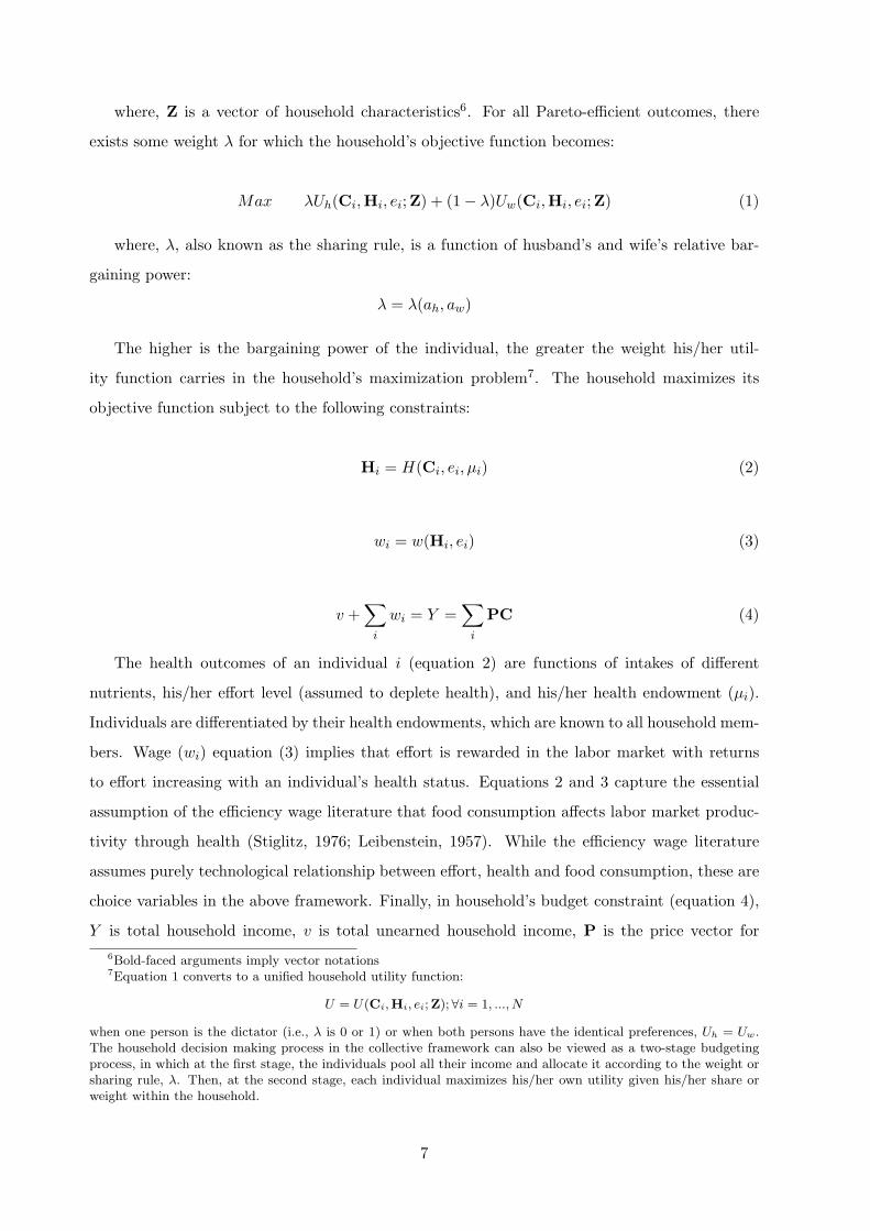
where, Z is a vector of household characteristics6. For all Pareto-efficient outcomes, there

exists some weight λ for which the household’s objective function becomes:

Max λUh(Ci,Hi, ei;Z) + (1− λ)Uw(Ci,Hi, ei;Z) (1)

where, λ, also known as the sharing rule, is a function of husband’s and wife’s relative bar-

gaining power:

λ = λ(ah, aw)

The higher is the bargaining power of the individual, the greater the weight his/her util-

ity function carries in the household’s maximization problem7. The household maximizes its

objective function subject to the following constraints:

Hi = H(Ci, ei, µi) (2)

wi = w(Hi, ei) (3)

v +∑i

wi = Y =∑i

PC (4)

The health outcomes of an individual i (equation 2) are functions of intakes of different

nutrients, his/her effort level (assumed to deplete health), and his/her health endowment (µi).

Individuals are differentiated by their health endowments, which are known to all household mem-

bers. Wage (wi) equation (3) implies that effort is rewarded in the labor market with returns

to effort increasing with an individual’s health status. Equations 2 and 3 capture the essential

assumption of the efficiency wage literature that food consumption affects labor market produc-

tivity through health (Stiglitz, 1976; Leibenstein, 1957). While the efficiency wage literature

assumes purely technological relationship between effort, health and food consumption, these are

choice variables in the above framework. Finally, in household’s budget constraint (equation 4),

Y is total household income, v is total unearned household income, P is the price vector for

6Bold-faced arguments imply vector notations7Equation 1 converts to a unified household utility function:

U = U(Ci,Hi, ei;Z);∀i = 1, ..., N

when one person is the dictator (i.e., λ is 0 or 1) or when both persons have the identical preferences, Uh = Uw.The household decision making process in the collective framework can also be viewed as a two-stage budgetingprocess, in which at the first stage, the individuals pool all their income and allocate it according to the weight orsharing rule, λ. Then, at the second stage, each individual maximizes his/her own utility given his/her share orweight within the household.

7

different nutrients and leisure, and total labor time is normalized to 1.

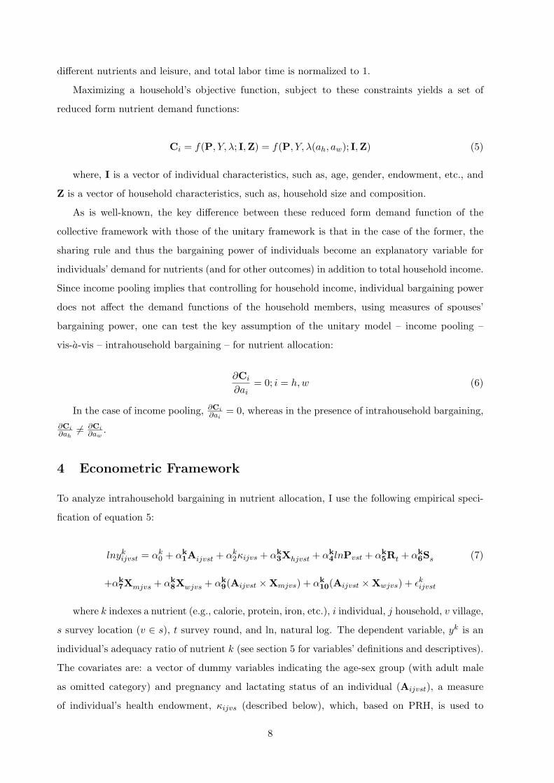
Maximizing a household’s objective function, subject to these constraints yields a set of

reduced form nutrient demand functions:

Ci = f(P, Y, λ; I,Z) = f(P, Y, λ(ah, aw); I,Z) (5)

where, I is a vector of individual characteristics, such as, age, gender, endowment, etc., and

Z is a vector of household characteristics, such as, household size and composition.

As is well-known, the key difference between these reduced form demand function of the

collective framework with those of the unitary framework is that in the case of the former, the

sharing rule and thus the bargaining power of individuals become an explanatory variable for

individuals’ demand for nutrients (and for other outcomes) in addition to total household income.

Since income pooling implies that controlling for household income, individual bargaining power

does not affect the demand functions of the household members, using measures of spouses’

bargaining power, one can test the key assumption of the unitary model – income pooling –

vis-a-vis – intrahousehold bargaining – for nutrient allocation:

∂Ci

∂ai= 0; i = h,w (6)

In the case of income pooling, ∂Ci∂ai

= 0, whereas in the presence of intrahousehold bargaining,

∂Ci∂ah

= ∂Ci∂aw

.

4 Econometric Framework

To analyze intrahousehold bargaining in nutrient allocation, I use the following empirical speci-

fication of equation 5:

lnykijvst = αk0 + αk

1Aijvst + αk2κijvs + αk

3Xhjvst + αk4lnPvst + αk

5Rt + αk6Ss (7)

+αk7Xmjvs + αk

8Xwjvs + αk9(Aijvst ×Xmjvs) + αk

10(Aijvst ×Xwjvs) + ϵkijvst

where k indexes a nutrient (e.g., calorie, protein, iron, etc.), i individual, j household, v village,

s survey location (v ∈ s), t survey round, and ln, natural log. The dependent variable, yk is an

individual’s adequacy ratio of nutrient k (see section 5 for variables’ definitions and descriptives).

The covariates are: a vector of dummy variables indicating the age-sex group (with adult male

as omitted category) and pregnancy and lactating status of an individual (Aijvst), a measure

of individual’s health endowment, κijvs (described below), which, based on PRH, is used to

8

control for any potential nutrition, health, and labor market linkages, time variant and invariant

household characteristics (Xhjvst), village food prices (Pvst), dummy variables for survey round

(Rt) and sites (Ss), and characteristics of household head (Xmjvs) and his wife (Xwjvs).

Controlling for individual and household characteristics, gender difference in nutrient ade-

quacy ratios will be reflected in the coefficient vector αk1. Controlling for household composition,

any potential household scale (dis)economies (Deaton and Paxson, 1998) that might make indi-

viduals of a larger household (worse)better-off in nutrient consumption (at the same level of per

capita expenditure) will be captured by the household size. Controlling for aggregate household

resources, spouses’ characteristics are of interest from intrahousehold bargaining perspective.

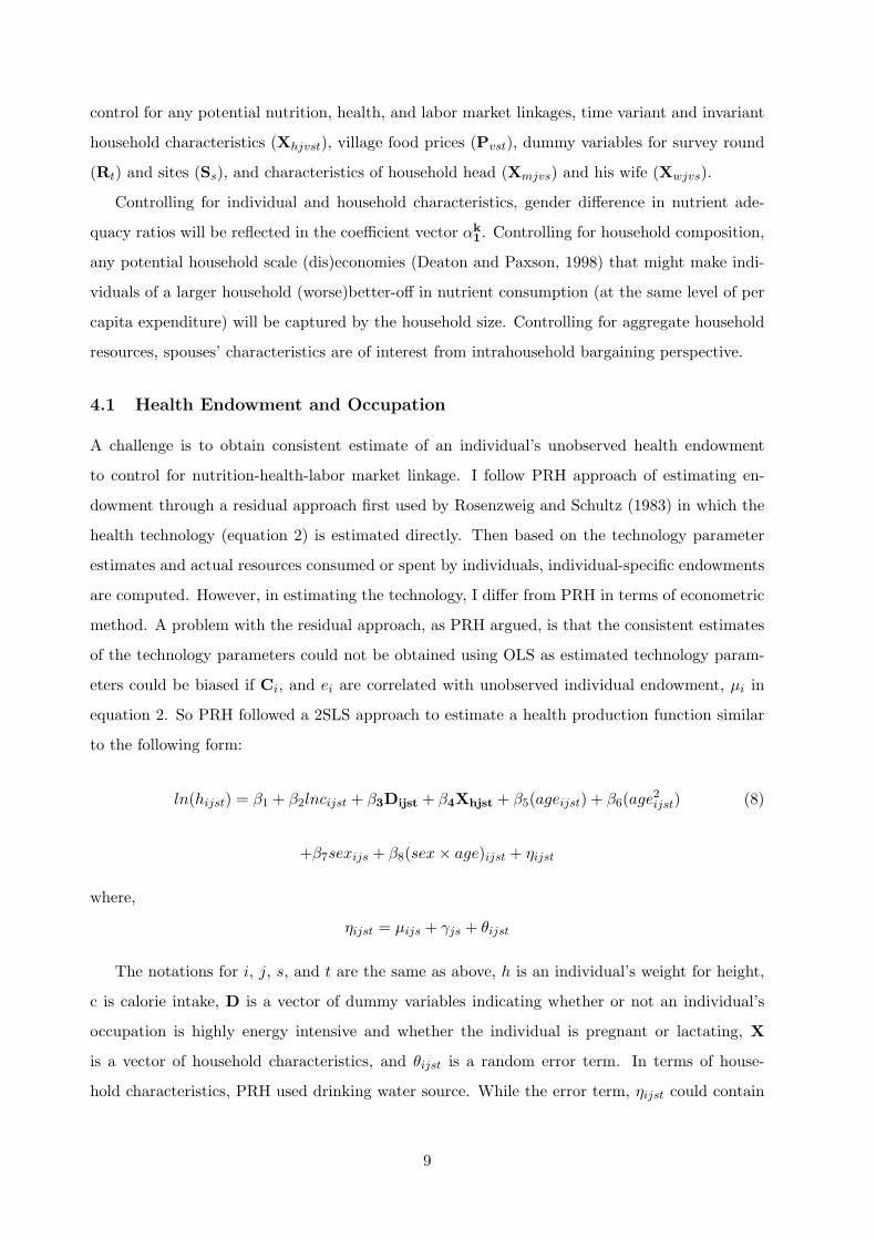
4.1 Health Endowment and Occupation

A challenge is to obtain consistent estimate of an individual’s unobserved health endowment

to control for nutrition-health-labor market linkage. I follow PRH approach of estimating en-

dowment through a residual approach first used by Rosenzweig and Schultz (1983) in which the

health technology (equation 2) is estimated directly. Then based on the technology parameter

estimates and actual resources consumed or spent by individuals, individual-specific endowments

are computed. However, in estimating the technology, I differ from PRH in terms of econometric

method. A problem with the residual approach, as PRH argued, is that the consistent estimates

of the technology parameters could not be obtained using OLS as estimated technology param-

eters could be biased if Ci, and ei are correlated with unobserved individual endowment, µi in

equation 2. So PRH followed a 2SLS approach to estimate a health production function similar

to the following form:

ln(hijst) = β1 + β2lncijst + β3Dijst + β4Xhjst + β5(ageijst) + β6(age2ijst) (8)

+β7sexijs + β8(sex× age)ijst + ηijst

where,

ηijst = µijs + γjs + θijst

The notations for i, j, s, and t are the same as above, h is an individual’s weight for height,

c is calorie intake, D is a vector of dummy variables indicating whether or not an individual’s

occupation is highly energy intensive and whether the individual is pregnant or lactating, X

is a vector of household characteristics, and θijst is a random error term. In terms of house-

hold characteristics, PRH used drinking water source. While the error term, ηijst could contain

9

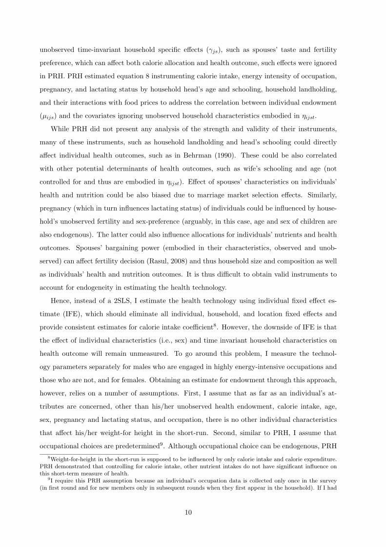
unobserved time-invariant household specific effects (γjs), such as spouses’ taste and fertility

preference, which can affect both calorie allocation and health outcome, such effects were ignored

in PRH. PRH estimated equation 8 instrumenting calorie intake, energy intensity of occupation,

pregnancy, and lactating status by household head’s age and schooling, household landholding,

and their interactions with food prices to address the correlation between individual endowment

(µijs) and the covariates ignoring unobserved household characteristics embodied in ηijst.

While PRH did not present any analysis of the strength and validity of their instruments,

many of these instruments, such as household landholding and head’s schooling could directly

affect individual health outcomes, such as in Behrman (1990). These could be also correlated

with other potential determinants of health outcomes, such as wife’s schooling and age (not

controlled for and thus are embodied in ηijst). Effect of spouses’ characteristics on individuals’

health and nutrition could be also biased due to marriage market selection effects. Similarly,

pregnancy (which in turn influences lactating status) of individuals could be influenced by house-

hold’s unobserved fertility and sex-preference (arguably, in this case, age and sex of children are

also endogenous). The latter could also influence allocations for individuals’ nutrients and health

outcomes. Spouses’ bargaining power (embodied in their characteristics, observed and unob-

served) can affect fertility decision (Rasul, 2008) and thus household size and composition as well

as individuals’ health and nutrition outcomes. It is thus difficult to obtain valid instruments to

account for endogeneity in estimating the health technology.

Hence, instead of a 2SLS, I estimate the health technology using individual fixed effect es-

timate (IFE), which should eliminate all individual, household, and location fixed effects and

provide consistent estimates for calorie intake coefficient8. However, the downside of IFE is that

the effect of individual characteristics (i.e., sex) and time invariant household characteristics on

health outcome will remain unmeasured. To go around this problem, I measure the technol-

ogy parameters separately for males who are engaged in highly energy-intensive occupations and

those who are not, and for females. Obtaining an estimate for endowment through this approach,

however, relies on a number of assumptions. First, I assume that as far as an individual’s at-

tributes are concerned, other than his/her unobserved health endowment, calorie intake, age,

sex, pregnancy and lactating status, and occupation, there is no other individual characteristics

that affect his/her weight-for height in the short-run. Second, similar to PRH, I assume that

occupational choices are predetermined9. Although occupational choice can be endogenous, PRH

8Weight-for-height in the short-run is supposed to be influenced by only calorie intake and calorie expenditure.PRH demonstrated that controlling for calorie intake, other nutrient intakes do not have significant influence onthis short-term measure of health.

9I require this PRH assumption because an individual’s occupation data is collected only once in the survey(in first round and for new members only in subsequent rounds when they first appear in the household). If I had

10

argued that they are given by social norms that limit females’ outside labor market participation,

while men are engaged in energy-intensive labor market activities. Thus, few women are engaged

in plowing in India, while in Bangladesh no women are observed to pull rickshaw10. As a conse-

quence of gender-segregated occupations, as PRH demonstrated, health endowment in the labor

market matters only for males. Behrman and Deolalikar (1989) and Sahn and Alderman (1988)

also find that health and calorie consumption have significant positive effects on men’s but not

on women’s wage rates. So for females, I estimate the technology without differentiating them

based on the energy-intensity of their occupation. Moreover, consistent with PRH assumption,

there are only a very few females engaged in high energy intensive occupations in the data (see

Section 5). Thus, for each of these three categories, I estimate the following health technology

function using IFE:

∆ln(hijst) = β1IFE + β2IFE∆lncijst + β3IFE∆ln(ageijst) + β4IFE∆[ln(ageijst)]2+ (9)

β5IFE∆Xhjst +

∑t

γt∆Rt +∆uijst

where household characteristic vector, Xhjst, includes monthly per capita expenditure and its

square, per capita household landholding, and household size, all in logs, share of different demo-

graphic composition of the household, Rt are survey round dummies to control for any potential

seasonal effects on health outcomes, and ∆ indicates deviation of an individual’s observation in a

given round from its mean (over four rounds). In estimating equation 9 for females, I also include

pregnancy and lactating dummies.

Applying IFE estimates of the parameters for calorie intake, age and its square, and household

characteristics from equation 9 to the individual data of the corresponding variables, I obtain

estimated log weight for height ( ˆln(h)) for each individual who belongs to any of the three above

sex-occupation categories. Deducting this estimated value from the observed value of log weight

for height (lnh) yields a health measurement that includes an individual’s unobserved health

endowment (µ) and an aggregate unmeasured effect of time-invariant household characteristics

(ρ) (e.g. the effect of spouses’ characteristics, such as education, assets, unobserved preferences,

household landholding, short-run time-invariant living and hygiene conditions, drinking water

source, etc. as discussed above):

time-varying occupation data, I could obtain consistent estimate of its impact on health using IFE without thisassumption.

10Morris (1997) finds that traditions in Bangladesh often inhibit a woman’s ability to obtain employment outsideof home. Purdah, or female seclusion, is an Islamic tradition routinely practiced in Bangladesh among the Muslimmajority, which limits women’s labor market participation.

11

ln(h)− ˆln(h) = µ+ ρ = κ

As I have four rounds of data for an individual, I average κ over four rounds and use it

as a proxy measure for an individual’s health endowment in equation 7. Obviously, estimating

equation 7 using OLS will be problematic as the health measure κ will include the effect of

unmeasured household characteristics, but these should be eliminated by estimating equation

(7) using household fixed effect. Thus, the measure κ along with other factors discussed below

motivates HFE estimation of equation 7.

4.2 Test of the Unitary Model and Household Fixed Effect

Based on OLS estimate of equation 7, a test for unitary model will be the tests of the restrictions

that for an individual’s nutrient allocation (conditional on individual and household charac-

teristics), the effect of a head’s characteristics will be same as the effect of the corresponding

characteristics of his wife. Thus, for the adult male (omitted category), the restrictions are:

αk7e = αk

8e , e = assets, education (10)

for each of the remaining age-gender category (g ∈ G):

αk7e + αk

9eg= αk

8e + αk10eg

(11)

for adolescent (adolf) and adult (adulf) pregnant (preg) and lactating (lact) women:

αk7e + αk

9ed+ αk

9ep= αk

8e + αk10ed

+ αk10ep

, d = adolf, adulf ; p = preg, lact (12)

and, for each of the age-gender-pregnancy-lactating category, relative to adult males:

αk9eg

= αk10eg

(13)

αk9ed

+ αk9ep

= αk10ed

+ αk10ep

The OLS estimates, however, have a number of econometric concerns, which in turn motivate

HFE estimation. In addition to the effect of ρ in the endowment measure κ, household size and

composition could be potentially endogenous to the household’s unobserved fertility preference,

the latter could also influence the nutrient allocation decisions. If households have preference for

sons and follow a male-biased stopping rule that could influence household size and composition.

12

This could result in girls living in bigger families (with more siblings) than boys (Barcellos

et al., 2010). As already mentioned, bigger families may have scale (dis)economies that can

affect individuals’ nutrient intakes. To the extent the unobserved fertility preference is time-

invariant, it could be eliminated by HFE method. Household income (proxied by expenditure) is

also potentially endogenous as both nutrient consumption and health endowment of individuals

may affect household income. In the literature, household expenditure is often instrumented by

household landholding. However, Behrman and Deolalikar (1990) distinguish the effect of current

income vis-a-vis permanent income on nutrient intakes, arguing that if households protect their

nutrient intakes from short-term fluctuations, the income elasticities of nutrient intakes would be

biased downward relative to the true household response to permanent income changes. They

find that the effect of nutrient intake responses to both current and permanent income are quite

small. Following Behrman and Deolalikar (1990), I use both current and permanent income

(proxied by per capita landholding) measures as explanatory variables. If a household’s nutrient

allocation decision based on an individual’s endowment and labor market productivity is time

invariant, then this unobserved household characteristic that might influence household income

is eliminated in HFE estimates.

Spouses’ assets and education at marriage could be correlated with their unobserved charac-

teristics, such as their preference for children’s (of particular sex) nutrition and health, which in

turn could be correlated with household formation through marriage market selection. For in-

stance, a man (woman) who wants healthy children may also choose an educated and/or wealthy

wife (husband). So a wife’s (man’s) education and/or assets may appear to influence a child’s

nutrition, even if for the same man (woman) changes in wife’s (husband’s) assets or education

would not affect the child’s outcome. The effect of a wife’s (husband’s) bargaining measures

on child’s nutritional allocation will be overestimated if husband (wife) with a high taste for

children’s nutrition tend to choose educated and/or wealthier spouse. This could in turn lead

to erroneous rejection of unitary model in favor of intrahousehold bargaining. Hence, another

motivation for HFE is to eliminate spouses’ time-invariant unobserved characteristics that could

be correlated with their bargaining measures and could influence individuals’ nutrient allocations.

The survey, as described in the next section, was conducted in four rounds. Using within

household variation of individuals’ nutrient intakes in different rounds, and variation of time

varying household characteristics across rounds, I estimate the following HFE version of equation

(7):

∆lnykijvst = αk0FE

+ αk1FE

∆Aijvst + αk2∆κijvs + αk

3FE∆Xhjvst + αk

4FE∆lnPvst (14)

+αk5FE

∆Rt+ αk

9FE∆(Aijvst ×Xmjvs) + αk

10FE∆(Aijvst ×Xwjvs) + ∆ϵkijvst

13

where ∆ indicates deviation of observations from household mean. However, eliminating

household fixed effects also eliminate time-invariant observable household characteristics, in my

case which include spouses’ bargaining measures. Therefore, to assess intrahousehold bargaining,

I can now only test the restrictions in equation 13. Moreover, the data is collected over four

rounds within a year, so there will be very limited variation of household size, demographic

composition, and per capita landholding (as landholding data is only from first round) across

rounds. So the effects of these variables could be imprecisely estimated. The HFE estimates

will be also based on a restricted sample of households that have at least one member of each of

the age-sex group under consideration. Also, the noise to signal ratio is likely to increase due to

differencing.

Finally, as I analyze intrahousehold bargaining for a number of nutrients, the likelihood that

no gender differences are found along any margin is very low. So the results might be biased

towards finding discrimination. Moreover, individuals’ consumption of one nutrient may affect

the consumption of others as typically they consume a food-bundle in which different food items

contain different nutrients in different proportions. To address these issues, adequacy ratios for

all nutrients under level specification 7 and HFE specification 14 are estimated simultaneously

in a seemingly unrelated regression (SUR) framework (henceforth, referred to as SURLS and

SURHFE , respectively).

5 Data and Descriptives

I use an innovative household survey data from the International Food Policy Research Institute

(IFPRI). The data come from four rounds of surveys at four month intervals during 1996-97

(Round 1: June-September, 1996; Round 2: October-December, 1996; Round 3: February-May,

1997; and Round 4: June-September, 1997) in 47 villages from three sites in four districts of

Bangladesh11. The survey objective was to evaluate the impact of commercial vegetable produc-

tion in Saturia (site 1), polyculture fish production in household-owned ponds in Mymensingh

(site 2), and polyculture fish production in group-managed ponds in Jessore (site 3) on house-

hold income, nutrition, and time allocation. In each site, villages were categorized into program

villages (A villages) where the technology was already introduced and comparable control vil-

lages (B villages) where the technology was yet to be introduced. From each of these categories,

surveyed A and B villages were randomly selected. A household census was conducted in all

the randomly selected A and B villages, from which households of two categories (adopters and

11Bangladesh is divided into six divisions. A division is then divided into districts. A district is composed ofseveral thanas. Thanas are divided into unions. A union is composed of several villages.

14

non-adopters in A villages, and households who expressed interest to adopt if the technology is

introduced and who were uninterested in B villages) were selected12.

The survey questionnaire was administered to 5,541 individuals in 955 rural households in each

round who were selected through this multi-stage sampling approach. The survey collected de-

tailed information on demographic characteristics, agricultural production, other income-earning

activities, expenditure patterns, time allocation, individual food intakes, health, morbidity, and

education. It also collected information on family background, marriage history, assets at mar-

riage, transfers at marriage, inheritance, women mobility, and empowerment.

IFPRI sampling required that the households were representative of adopters and non-adopter

households in A villages and likely adopters and likely non-adopters in B villages, and not nec-

essarily representatives of rural Bangladeshi households. Nonetheless, a comparison of IFPRI

sample with that of 1995-96 National Household Expenditure Survey (HES) of Bangladesh Bu-

reau of Statistics of the Government of Bangladesh indicates that the IFPRI sample is broadly

comparable to the nationally representative HES rural sample of 5,020 households based on

household size, per capita expenditure, landholding, and poverty rates (Table 1).

5.1 Variables and Descriptives

Table 1 provides the descriptive statistics of the variables used in the econometric analysis, and

the variables are described below.

Survey round and site dummies: Survey round dummies (with 4th round omitted) are

included to control for any agricultural seasonality that may affect nutrient consumption as in

lean seasons there may be lack of food availability and labor market activities that can affect

household food expenditure and income. As there are two major rice cultivation seasons, there

are also two lean seasons that reduce employment and income earning opportunities. The major

lean season is from mid-September to mid-November preceding the Aman harvest, which falls in

round 2. The other lean season falls in round 3, which is from mid-March to mid-April, prior

to Boro harvest13. Site dummies (with Jessore as omitted site) are included to control for any

location specific effects, such as infrastructure, location endowment, market condition, health

facility, etc., which may affect income earning opportunities, food availability and prices, health,

and nutrition.

Village prices: The survey collected data on household food expenditure and quantity

12The IFPRI evaluation concluded that adoption of these programs, had neither improved the micronutrientstatus of the adopting households through better quality diet nor increased their incomes. For a detailed descriptionof the survey, see (IFRPI-BIDS-INFS, 1998).

13Aman and Boro are the rice grown in monsoon and dry season, respectively.

15

purchased of a wide range of food items, which were further classified into 17 different food

groups. Village prices are proxied by village level mean unit value for each of these food groups,

which are constructed by averaging the household level unit value of these food groups within

each village. I control for log village price of rice, pulses, big fish, small fish, and egg in the

regression functions14. Table 1 indicates substantial variation of village prices across rounds,

while high and low prices of different food groups are observed at different times of the year.

For instance, while the mean rice price is lowest in round 2 and highest in round 3, for pulses

the highest is observed in round 2 and lowest in round 4, implying seasonality (if any) differs for

different food groups.

Household size and composition: Household size is based on number of individuals

present in the household in each round. Consistent with nutritional requirements at different

stages of life-cycle and activity patterns, males and females are categorized into: children (< 10

years), adolescents (10 ≤ age < 18 years), and adults (≥ 18 years). Dummies for each of these

six age-sex categories (with adult male as omitted category) and a dummy for whether a female

is pregnant or not, or lactating or not in a given round are used in the econometric analysis. Log

household size and share of males and females in each of these age groups (with adult males’ share

as omitted category) are used to control for household size and composition. Compared to HES

sample, on average an IFPRI sample household is consists of 1-2 more people with highest share

of individuals in the adult category. As expected, there is very limited variation of household size

and composition across rounds within one year. The lactating women outnumbered pregnant

women, and these statuses vary across rounds.

Household landholding, expenditure, and poverty: Household landholding is a time

invariant variable for which information was collected in the first round. The share of landless

households is lower in IFPRI than in HES samples. The distribution of landholding is also less

unequal in IFPRI sample compared with HES sample with higher share of households with 1-7.5

acres in IFPRI sample. The mean per capita landholding in IFPRI sample is 0.23 acre (which

varies slightly across rounds due to limited variation in household size).

Both samples are similar in terms of mean per capita monthly expenditure, which varies

significantly across rounds (p-value of t-tests are not reported) in IFPRI sample with the lowest

value observed in round 2 and highest value in round 3.

The absolute and hard core poverty lines based on direct calorie intake (DCI) method are

2122 kcal and 1805 kcal per person per day, based on which the poverty incidence is higher in

IFPRI compared to HES sample. HES regional upper and lower poverty lines based on cost of

14A comprehensive set of village prices were initially included. Subsequently, I have included the food pricesthat appear to be significant most of the times for the set of nutrients analysed in this paper.

16

basic needs (CBN) approach in 1995-96 are Takas 593 and 492 in site 1, 529 and 484 in site 2,

592 and 499 in site 3, and 591 and 499 for national rural households. Comparison of HES sample

with site specific poverty incidence based on CBN gives a mixed picture with some sites in some

rounds having higher poverty rates compared to national rural average and vice versa. Similar to

monthly per capita expenditure, poverty incidence varies substantially across rounds. Based on

CBN, the highest poverty incidence in all sites are observed in round 2, while based on DCI, the

poverty peaks in round 3. As mentioned, round 2 contains the major lean season, while round 3

the minor one.

Spouses’ characteristics - age, education, and assets at marriage: On average, hus-

bands are about 8 years older than their wives. To focus on bargaining between husbands

and wives, following Quisumbing and Maluccio (2003), I restrict the sample to monogamous

households15 with husband and wife present and with no change in marital status (i.e., divorce,

separation, re-marriage, death, etc.) during the survey period. The resulting sample selection

bias (if any) would lead to a conservative estimate of bargaining effects as households in which

the disagreement between the spouses are the strongest would be more likely to split and are

thus absent in this sub-sample.

The marriage module of the survey asked the heads and their wives the assets they owned at

the time of their wedding. These assets included land, cattle, housing, food items, and durable

(jewelery, watch, clothes, and household utensils). The reported values of these assets at the

time of marriage were converted in 1996 taka using national consumer price index. Bangladeshi

wives had far less assets at the time of their marriage than their husbands primarily because their

value of landholding, housing, and cattle were much less than those of their husbands (see Table

1). The assets at marriage may suffer from measurement errors due to recalling information,

particularly for longer marriages. One option is to instrument spouses’ assets by their respective

family background information, such as the wealth of their parents. However, those measures

may also suffer from recall errors. Hence, I do not instrument these bargaining measures. To

the extent the measurement errors are white noise, the evidence of bargaining (if any) will be

an underestimation of the true bargaining effects. Education is measured by years of schooling.

The mean years of schooling of husbands is almost double of that of wives.

While spouses’ assets at marriage are my key bargaining measures, following Quisumbing and

Maluccio (2003), in the empirical analysis, I also include spouses’ age and age square to control

for cohort effects, and for the possibility that their age difference could be another source of

151% of households have two wives, while 4.5% are female headed with no husband, and 3% have head withouthis wife. 91% households are intact with both head and his spouse. Based on data availability of assets at marriage,my analysis contains almost 98% of these intact households, or, roughly 89% of the all surveyed households.

17

bargaining power that may be correlated with the education and assets measures. While spouses’

education are included as a potential bargaining source, its caveats are already discussed (see

section 2). My focus, however, is not to evaluate intrahousehold bargaining based on education,

but to control for any potential correlation between education and asset measures of bargaining.

Individual health and occupation: There is limited variation across rounds even in the

short-term health outcome measure, an individual’s weight (in kilograms) for height (in centime-

ters). Boys tend to do better than girls and adult males better than adult females, while this

gender difference reverses for the adolescent group. This might be indicative of some transitory

catch-up for females as they past childhood, which later disappears as they progress toward

adulthood.

As mentioned before, occupation data were collected once in the survey. These were coded

into 47 different occupations. Based on the metabolic constant (mc) provided for a detailed

list of activities for male and female in World Health Organization (1985), I classify the energy

intensity of occupations into high (mc > 4), medium (2.5 < mc ≤ 4), and low (mc ≤ 2.5)

category16. Energy intensity of occupation of different age-sex group vis-a-vis their energy intake

are further discussed below. As described in Section 4, both the energy intensity of occupation

and health outcome are utilized to construct the health endowment measure.

Calorie intake and energy-intensity of occupation: A useful feature of IFPRI survey

is that it provides individual food intake data for each round using a 24-hour recall methodology

asking the person with primary responsibility for preparing meals, about recipes prepared, ingre-

dients for those recipes and amounts eaten by various family members and guests. The survey

has information of quantity of individual intakes of about 200 food items (categorised into 17

food groups), which are converted into calories, protein, and micronutrients (vitamin A, vitamin

C, vitamin D, niacin, riboflavin, thiamine, folate, iron, and calcium).

Calorie intake data broadly resembles to PRH claim that gender difference in calorie allocation

is age-dependent and so is the gender difference in energy-intensity of occupations. To replicate

PRH finding in IFPRI sample, I first use PRH’s age-group classification ((age<6, 6≤age<12,

and age≥12). The mean calorie consumption (averaged over four rounds) across age-groups are

higher in IFPRI than in PRH sample (see Table 2). However, there is no significant gender

difference for the group less than <6 years. Conversely, consistent with PRH, I find significant

gender difference for the age-group ≥ 12 years. While PRH does not find any significant gender

16PRH cited the same source for classification of energy intensity of occupations but did not describe differentcut-off points of mc they used for their classification. Basal metabolic rate (BMR) for an individual is the amountof energy spent when the person is in sleep. Energy requirement for different activities per minute is BMR timesthe mc of that activity. For instance, mc for cleaning house for a female is 3, while that for digging earth for maleis 5.7.

18

difference for the age-group 6-12 years, I find this difference is small but significant. In line

with PRH, the within-household inequality in calorie distribution, measured by the coefficient of

variation, is higher among males than females (the difference is significant) for age-group ≥ 12

years, while this inequality is not significant for the groups <6 years and 6− 12 years.

Based on my age-group classification, I find that boys have about 100 calories more than

girls (the difference is significant at 5% level). There is neither a marked difference in energy

requirement of occupations for children, nor any significant difference between intrahousehold

inequality among boys compared to the inequality among girls based on coefficient of variation.

The gender difference in calorie allocation increases almost three-folds for adolescents compared

with that of children. Compared to 1% adolescent females, 18% adolescent males are engaged in

high energy-intensive occupation. Within household inequality for adolescent males is about 23%

higher than that for the adolescent females (significant at 5% level). Adult males receive about

700 calories more than adult females, which reflects the fact that more than half of the adult

males compared with only 2% adult females are engaged in high energy-intensive occupations.

Thus, the broad linkages between work-activity and calorie distribution as observed by PRH

tends to hold for these age-groups as well.

Nutrient Adequacy Ratio: While PRH’s focus was only on individual calorie intake,

individuals’ intakes of calorie and different nutrients17 are not very useful unless compared against

their requirements. I thus construct nutrient adequacy ratio for each of the k nutrients:

yki =Cki

RDAki

where, yki is individual i’s adequacy ratio of nutrient k, Cki is his/her daily consumption of nutrient

k, and RDAki is his/her recommended daily allowance (or requirement) of nutrient k based on

age, sex, pregnancy, and lactating status. The appendix provides a detailed description of how

the RDA figures for calorie and different nutrients are constructed. As discussed in the appendix,

for protein and iron, not only quantity but also quality matters. Protein from animal sources

are good quality protein, while iron from animal sources (also termed as haem-iron) have high

bio-availability and promotes bio-availability of iron from non-animal sources. Hence, in addition

to individual’s nutrient adequacy ratio, I also use an individual’s intake of animal protein as a

share of protein requirement and intake of haem iron as a share of total iron requirement as

17All foods are made up of a combination of macronutrients (protein, fat, carbohydrate) and micronutrients(vitamins and minerals). Macronutrients form the bulk of the diet and supply all the energy needed for the bodyfor body functions, growth, and physical activities. Macronutrients provide different amounts of energy, expressedin kilocalorie (loosely termed as calorie as well). Fat provides approximately twice as much energy (9Kcals/g) asthe same amount of protein or carbohydrate (4Kcals/g).

19

dependent variables in the empirical analysis.

5.2 Nonparametric Analysis

Sex difference in the adequacy ratio of different nutrients at each age are nonparametrically

(using locally weighted regression method, lowess with bandwidth 0.8) shown in Figures 1 and

2. These figures illustrate a number of points. First, sex disparity in adequacy ratio is least

observed for calorie and among the micronutrients, for niacin. As discussed in the appendix,

calorie requirement figures for children and adolescents are based on US National Child Health

Survey (NCHS) standard and not based on actual energy expenditure because of lack of data on

time allocation for these age groups. Only for these groups, the adequacy ratio seems to be less

than 1. This might imply that perhaps these groups are having calories based on their actual

energy expenditure (which is unobserved in the data), but still they are having calories less than

NCHS standards to meet their full long-term growth potentials. On the other hand, for the adults

for which the requirements are based on actual energy expenditure, the adequacy ratio for both

males and females are at or above 1. Calorie intakes of all ages are also most stable (compared

to other nutrients) across different rounds (as requirement figures are fixed, any movement in

adequacy ratio across rounds implies fluctuation in intakes). All these are consistent with the

view in nutrition literature that given the wide variety of sources to meet one’s calorie need, in

normal circumstances (i.e., without famine) an individual can always meet his/her calorie need

(World Health Organization, 1985).

Second, for most of the other nutrients, sex disparity is prominent, persistent, and often

widens for adolescents and adults compared with children. For vitamin A and D in some rounds,

at a relatively high age (above 70 or so), females’ adequacy ratio cross over males’. However,

this cross-over should be interpreted with caution due to the limited number of observations at

those ages (with number of males higher than females). Third, with the exception of protein

and vitamin C, nutrient deficiency is prominent across ages for all other nutrients with adequacy

ratio lower than 1. The situation is most alarming for iron, where both males and females across

ages are in deficiency, with females’ deficiency worse than males’. While protein adequacy ratio

is above 1 across all ages (with males’ ratio higher than females’), the good quality protein (i.e.,

protein from animal, dairy, and fish, jointly termed as animal protein) as a share of required

protein is very low. The situation is even worse for haem iron. Finally, (vertical) shift of these

age-adequacy profiles for most of the nutrients (and changes in shapes for some nutrients) across

rounds imply variation of individual intakes of these nutrients across rounds.

To illustrate the role of bargaining in intrahousehold nutrient allocation, lowess graphs of

20

calorie and calcium adequacy of different age-sex groups, as examples, are shown in Figure 3.

The left (right) panel shows intakes of different age-sex group at different levels of wife’s (head’s)

assets at marriage when head’s (wife’s) assets at marriage is zero. For calorie, most contrasting

pattern is reflected for female child. Her calorie adequacy ratio tends to increase with wife’s assets

but declines with husband’s assets. The rate of decline of female adolescent’s adequacy ratio is

also much faster with the increase in head’s assets as opposed to his wife’s assets. While male

adult’s adequacy ratio increases with the increase in head’s assets, a v-shaped pattern appears

for this adequacy ratio and wife’s assets.

For calcium, adult female’s intake initially increases and adult male’s intake decreases with

the increase in head’s assets. After a point, the female’s intake sharply declines while the opposite

is observed for the male’s intake. Conversely, the initial rate of increase of adult female’s intake

is faster with the increase in wife’s assets, and after a point the intake declines at a slower rate

with the increase in wife’s assets (compared to the increase in head’s assets). Adult male’s intake

appears to be negatively related with wife’s assets. The male child’s intake increases with head’s

assets. This intake moderately increases with the initial increase in wife’s assets and then tends

to decline.

All these contrasting relationships between individual intakes and spouses’ assets at marriage

motivate a more detailed empirical analysis of intrahousehold bargaining on individual nutrient

allocations in the following section.

6 Estimation

6.1 Calorie intake and health technology

Table 3 presents the estimates of the health technology (equation 9) for males engaged in highly

energy intensive occupations (HEIO) (as defined in the preceding section) and non-HEIO and

for females. OLS estimates are presented along with IFE estimates for comparison purpose. The

results imply three points. First, the role of calorie intake on individual’s health outcome is much

limited once unobserved individual and household fixed effects are accounted for. For each of

the three categories of individuals, the effect of calorie intake on health outcome is much higher

in OLS than IFE estimates, indicating upward bias in OLS estimates, presumably driven by

unobserved individual endowment and household characteristics (such as spouses’ tastes). For

males in HEIO, doubling calorie intake will increase their weights for heights by 5% in OLS

estimate, while the corresponding increase is only 0.67% in IFE estimate. Second, this effect

of calorie intake varies only marginally across individuals based on their energy intensity of

21

occupations. Doubling the calorie intake of males who are not engaged in HEIO and of females

will increase their weight for height by 0.54% compared to that by 0.67% for males in HEIO based

on IFE estimates. Third, comparison of IFE results with that of PRH (in which, doubling calorie

intake will increase the weight for height of individuals by about 13.6% in 2SLS estimate and

3% in OLS estimate), implies that PRH’s 2SLS estimate of calorie elasticity could be potentially

biased upward. As discussed above, the validity of PRH instruments is questionable as head’s

schooling seems to have a significant direct effect on males (non-HEIO) health outcome, while

wife’s education (not controlled in PRH) seems to positively and significantly18 affect females’

health outcomes in OLS estimates. These effects are not identifiable in IFE estimates as they

are absorbed in household fixed effects. Another PRH instrument, household landholding seems

to significantly affect males’ (in HEIO) health outcomes in IFE estimate. All these in turn may

imply that perhaps the inequality in calorie distribution due to inequality in energy intensity of

labor market activities is overemphasized in PRH analysis.

As regards other variables, economies of scale (in terms of household size, holding the house-

hold composition constant) in health production is observed for males (particularly for those in

non-HEIO) but not for females. Health outcomes for males in HEIO only slightly worsens (by

3%), while that for males not in HEIO and females slightly improves (by 1-3%) in round 1 and 2

compared with round 4 (results not shown). As discussed above, IFE estimates of the coefficients

of the health technology are used to construct a measure of unobserved health endowment, κ,

which is used in the nutrient demand equations discussed below.

6.2 Intrahousehold Bargaining and Nutrient Allocation

Calorie, Protein, and Vitamin A: Table 4 presents the SURLS and SURHFE estimates of

intrahousehold bargaining and allocation of calorie, protein, protein from animal sources (i.e.,

good quality protein), and vitamin A for boys, girls, male adolescents, female adolescents, female

adults, male adults (omitted category), pregnant, and lactating females. As SURLS estimates

could be biased (see Section 4), the analysis focuses on SURHFE estimates, while SURLS es-

timates are provided for comparison purposes. Spouses’ assets at marriage and schooling are

interacted with each of these age-gender-physical status categories to analyze whether a head’s

bargaining measures have significantly different effects on intrahousehold allocation of these nu-

trients than the corresponding bargaining measures of a wife. Given the caveats associated with

education as a bargaining measure, I focus on bargaining based on assets measures although

18Throughout the paper, ”significant” implies statistical significance at 10% level or lower, unless specificallymentioned otherwise.

22

I use spouses’ education and the corresponding interaction terms to control for any potential

correlation between education and assets of spouses.

Boys’ and girls’ calorie adequacy ratio are about 29% and 26% lower than that of adult

males in SURHFE estimate, implying that girls have about 3% higher calorie adequacy ratio

than boys. While adolescent males’ calorie adequacy ratio are about 5% lower than that of adult

males, there is no significant difference among the adequacy ratio of adolescent females, adult

females and adult males. This pattern of within age-group gender difference, however, reverses for

the allocation of protein, good quality protein19 and vitamin A. Within each of the age-groups,

a female’s adequacy ration is significantly lower than that of a male for each of these nutrients.

Compared to calorie adequacy ratio, the adequacy ratio for each of these nutrients for pregnant

and lactating women are much lower than that of adult males (with the exception of pregnant

womens’ vitamin A adequacy ratio).

A wife’s assets significantly and positively affect the calorie and protein adequacy ratio for

girls, calorie adequacy ratio for male adolescents, protein and vitamin A adequacy ratio and

allocation of good quality protein for female adolescents, and protein and vitamin A adequacy

ratio for female adults. For example, doubling a wife’s assets would increase the allocation of

good quality protein for female adolescents by 6%. A head’s assets, on the other hand, negatively

and significantly affect the allocation of good quality protein for boys, girls, male adolescents,

and female adolescents, and calorie adequacy ratio for male adolescents. For instance, doubling

a head’s asset would reduce the allocation of good quality protein for girls by 3% in household

fixed effect estimates. Tests of unitary model for the equality of the effects of head’s and wife’s

assets 20 (bottom panel of Table 4) provide evidence of significant intrahousehold bargaining for

allocation of calorie, protein, and good quality protein for girls, calorie and good quality protein

for male adolescents, total protein and good quality protein for female adolescents, and calorie

and total protein for female adults with a positive association between a wife’s assets and these

allocations.

The effect of individual health endowment (κ) implies compensation for protein and vitamin

A allocations with no significant effect on calorie allocation. Doubling an individual’s endowment

will roughly reduce the adequacy ratio of protein by 1.7% and vitamin A by 1.6%. Apart from

vitamin A, at the initial level of income, individual intakes of these nutrients increase with the

19The term ”adequacy ratio” is loosely used for good quality protein and haem-iron, for which it measures intakeof good quality protein as a share of total protein requirement, and intake of haem iron as a share of total ironrequirement.

20I test the complete set of restrictions for bargaining described in equations 10, 11, 12, and 13 for educationand asset measures for each of the age-sex-pregnancy-lactating group, which are available upon request. As I focuson assets as the key bargaining measure, the discussion concentrates on the restrictions in equation 13 based onassets as the results are comparable between SURLS and SURHFE models.

23

increase in household income. The increase is most prominent for good quality protein. Although

inelastic, the expenditure elasticity at the initial level of income is higher for total protein than

total calorie intake. Household economies of scale appears to be significant for calorie and protein

(in OLS estimates) and for vitamin A (in HFE estimates) intakes. In terms of agricultural

seasonality, individual intakes of calorie, protein and good quality protein appear to be lowest in

round 3.

Vitamin C, D and Iron: Table 5 presents the results of intrahousehold bargaining and

individual allocation of vitamin C, D, iron, and haem iron. The adequacy ratio for all age-sex

groups and pregnant and lactating women are significantly lower than that for adult males for

each of these nutrients. Within each age-group, the adequacy ratio for males are significantly

higher than that for females for each of these nutrients, while pregnant and lactating women have

significantly lower adequacy ratio than adult males. For instance, based on fixed effect estimates

adult females’ iron adequacy ratio are about 93% lower than adult males’, while the former’s

haem iron share is 108% lower than that of adult males. A pregnant woman’s iron adequacy

ration is 171% lower than that of an adult male, while her haem iron allocation (as a share of

her total iron requirement) is about 178% lower than that for an adult male. Similarly, a female

adolescent’s iron adequacy ration is about 18% lower than that of a male adolescent, while her

haem iron share is about 25% lower than that of a male adolescent. The degree of sex-disparity

in iron allocation is comparatively lower among children as a boy’s iron adequacy ration and

haem iron share are about 9% higher than those of a girl. Among children, the magnitude of

sex-disparity appears to be higher for vitamin C and D than iron.

Significant intrahousehold bargaining is observed for haem iron share for boys, male and

female adolescents, and for lactating adolescents (see bottom panel of Table 5). A head’s assets

negatively affect the haem iron allocation for boys and adolescents, while a wife’s assets has the

opposite effect. For instance, doubling a wife’s assets would increase the haem iron share by

10% for female adolescents while the corresponding increase in head’s assets would decrease it

by 1.5%.

The effect of κ implies that households tend to compensate for lower endowments. Doubling

an individual’s endowment would reduce his/her adequacy ratio of vitamin C by 1%, vitamin

D by 2%, iron by 3%, and haem iron share by 2%, approximately. Among these nutrients, the

expenditure elasticity seems to be highest for vitamin D at the initial level of income, while

household economies of scale appears to be significant for vitamin C and iron intakes. Vitamin

C intake appears to be significantly lower in all three rounds compared to round 4, while vitamin

D consumption is about 16% lower in round 1 and 39% lower in round 3 than that in round 4.

24

Calcium, Niacin, Riboflavin, Thiamin, and Folate: Table 6 presents the results for this

last set of nutrients. Based on fixed effect estimates, calcium adequacy ratio for boys are 15%

higher than that for girls. The corresponding ratio for male adolescents are 11% higher than that

for female adolescents, and adult females’ calcium adequacy ratio are 32% lower than that of adult

males. Compared with adult males, the situation for pregnant (83% lower) and lactating females

(74% lower) are even worse. While female adults’ niacin adequacy ratio are not significantly

different from that of male adults, both pregnant and lactating women have 19% and 14% lower

niacin adequacy ratio than that of adult males. Sex disparity among children is also significant

with boys having higher niacin adequacy ration than girls. While pregnant women’s riboflavin

adequacy ratio are not significantly different from that of adult males, lactating women’s adequacy

ratio are 8% lower and female adults’ ratio 13% lower than that of adult males. Boys’ riboflavin

adequacy ratio are 9% higher than girls’. Similar pattern of sex disparity across all age-sex-

physical status groups is observed for thiamin and folate as well. For folate, while girls’ adequacy

ratio is not significantly different from that of adult males, boys’ adequacy ratio are about 10%

higher than that of adult males (and girls).

Evidence of significant intrahousehold bargaining appears (bottom panel of Table 6) for cal-

cium allocation for male and female adolescents and female adults and riboflavin and thiamin

allocations for male adolescents. A wife’s assets as opposed to head’s assets, positively affect each

of these allocations. For instance, doubling a wife’s assets would increase the calcium adequacy

ratio for adult females by 4%, while the effect of corresponding increase in head’s assets is not

significantly different from zero.

Allocation of these nutrients also imply that households tend to compensate for low individual

health endowments. Although inelastic, intakes of niacin and thiamin are positively associated

with the increase in household expenditure at lower level of expenditure. OLS estimates also

indicate significant economies of scale for individual consumption of these nutrients within the

household. There does not appear to be a consistent pattern of seasonality, perhaps because

seasonality varies for different foods. Compared to round 4, calcium intake is about 6% higher

in round 1, niacin intake is about 7% higher in round 2 and 4% higher in round 3, riboflavin

intake is 6.5% lower in round 3, folate intake is about 13% lower in round 3, and thiamin intake

is about 9% higher in round 3.

25

7 Summary and Conclusion

In light of the growing concern about micronutrient malnutrition as a critical public policy issue,

I attempt to extend the previous literature on intrahousehold food distribution by analyzing

intrahousehold nutrient allocation in a bargaining framework. While the focus of the previous

work has been on calorie allocation, I demonstrate that calorie intake may not necessarily be

a sufficient metric of nutrient adequacy as micronutrient deficiency can co-exist with calorie

adequacy. The gender disparity is more prominent in intrahousehold allocation of a range of

critical nutrients than calorie allocation. Pregnant and lactating women appear to be most

vulnerable as their intakes fall far short of their elevated requirements, which in turn might lead

to nutrient deficiency of the newborns.

Previous work on intrahousehold food distribution has adopted a unitary framework, which

has been rejected empirically for a wide range of outcomes in recent decades. PRH, an influential

work in this genre, further have demonstrated that food distribution in a poor economy like

Bangladesh is due to gender-disparity in the energy intensity of labor market activities in which

health influences labor market productivity and returns for males but not for females. However,

the individual fixed effect estimates of health technology in this paper indicate that PRH claim

might be overemphasized as their estimate of the effect of calorie on individual’s health outcomes

might be biased upward due to unobserved household fixed effects. These unobserved effects also

question the validity of PRH instruments used in reaching their conclusion. Moreover, as the

nutrition literature suggests, while calorie intake is a direct function of calorie expenditure and

thus of energy intensity of labor market activities, various nutrients analyzed in this paper need

not.

In a bargaining framework, controlling for potential marriage market selection and unob-

served household fixed effects, I demonstrate evidence of intrahousehold bargaining and positive

effect of a wife’s bargaining power as opposed to her husband’s in the allocation of a number

of critical nutrients for children and adolescents of both sexes and for adult females. Thus, my

policy implication fundamentally differs from that based on a unitary framework. Based on a

unitary framework, a key policy paradigm of the previous literature is to increase energy-intensive

labor market opportunities for women, or to achieve economic development by transforming work

activities to those in which linkages between food consumption and productivity are weak, which

however, might increase within-group inequality for women due to wider variation in their eco-

nomic activities. On the other hand, my findings imply that for any given level of economic

development and household income, gender disparity (both between the sexes and within the

adult women group) could be potentially reduced through increased women’s bargaining power

26

within the household achieved through various legal and policy changes that grant women more

control over resources. This policy implication is consistent with a number of studies that pro-

vide evidence that more control of resources by women leads to an improvement in child health,

nutrition, education, and on women’s own well-being. Moreover, women’s participation in the

labor market, a key policy lever in the unitary framework itself is endogenous, and is an outcome

of intrahousehold bargaining.

However, the change in a woman’s bargaining power may affect marriages (and perhaps

divorces). The measure of bargaining power used in this paper (assets at marriage) is largely

determined by parental wealth, and in this society the norm is that parents arrange marriages

for their offspring. Thus, future work perhaps could focus on how the policy change leading to

increased female controls of resources could potentially affect household formation and dissolution

and not just intrahousehold allocation in a traditional poor rural society.

Acknowledgements:

I thank Richard Blundell, Andrew Chesher, Imran Rasul, Sonia Bhalotra, Giacomo de Giorgi

for their valuable comments and suggestions. I also thank Howarth Bouis, Wahid Quabili, and

Agnes Quisumbing in helping me accessing the IFPRI data and with numerous queries. All the

remaining errors are mine.

References

Adato, M., de la Briere, B., Mindek, D., Quisumbing, A. R., 2003. The Impact of PROGRESA

on Women’s Status and Intrahousehold Relations. In: Quisumbing, A. R. (Ed.), Household De-

cisions, Gender, and Development. International Food Policy Research Institute, Washington,

D.C.

Barcellos, S. H., Carvalho, L., Lleras-Muney, A., 2010. Child Gender and Parental Investment in

India: Are Boys and Girls Treated Differently, mimeo, Rand and UCLA.

Bardhan, P. K., 1974. On Life and Death Questions. Economic and Political Weekly (Special

Issue).

Becker, G. S., 1973. A Theory of Marriage: Part I. Journal of Political Economy 81 (4), 813–846.

Behrman, J., 1990. Intrahousehold Allocation of Nutrients and Gender Effects: A Survey of

27

Structural and Reduced Form Estimates. In: Osmani, S. R. (Ed.), Nutrition and Poverty.

Oxford University Press, Oxford.

Behrman, J., 1997. Intrahousehold Distribution and the Family. In: Rosenzweig, M. R., Stark,

O. (Eds.), Handbook of Population and Family Economics. Handbooks in Economics series.

Elsevier Science, Amsterdam, pp. 125–187.

Behrman, J. R., 1988. Nutrition, Health, Birth Order and Seasonality: Intrahousehold Allocation

in Rural India. Journal of Development Economics 28, 43–63.

Behrman, J. R., Deolalikar, A. B., 1989. ”Is Variety the Spice of Life? Implications for Calorie

Intake”. The Review of Economics and Statistics 71 (4), 666–672.

Behrman, J. R., Deolalikar, A. B., 1990. ”The Intrahousehold Demand for Nutrients in Rural

South India: Individual Estimates, Fixed Effects, and Permanent Income”. Journal of Human

Resources 25 (4), 665–696.

Bouis, H. E., Haddad, L. J., Kennedy, E., 1992. Does It Matter How We Survey Demand for

Food? Evidence from Kenya and the Philippines. Food Policy 17 (5), 349–360.

Bourguignon, F., Browning, M., Chiappori, P.-A., Lechene, V., 1993. Intrahousehold Allocation

of Consumption: A Model and Some Evidence from French Data. Annales D’Economie et de

Statistique 29, 137–56.

Bourguignon, F., Browning, M., Chiappori, P.-A., Lechene, V., 1994. Incomes and Outcomes: a

Structural Model of Intra-Household Allocation. Journal of Political Economy 102 (6), 1067–

1096.

Chiappori, P.-A., 1988. Rational Household Labor Supply. Econometrica 56, 63–89.

Chiappori, P.-A., 1992. Collective Labor Supply and Welfare. Journal of Political Economy 100,

437–67.

Deaton, A., Paxson, C., 1998. Economies of Scale, Household Size, and the Demand for Food.

Journal of Political Economy 106 (5), 897–930.

Deolalikar, A. B., 1988. Do Health and Nutrition Influence Labor Productivity in Agriculture?

Econometric Estimates for Rural India. Review of Economics and Statistics 70, 406–413.

Doss, C., 1999. Intrahousehold Resource Allocation in Ghana: The Impact of Distribution of

Asset Ownership within the Household. In: Peters, G. H., von Braun, J. (Eds.), Food Security,

28

Diversification and Resource Management: Refocusing the Role of Agriculture? Dartmouth

Publishing, Aldershot, UK.

Folbre, N., 1984. Market Opportunities, Genetic Endowments, and Intrafamily Resource Distri-

bution: Comment. American Economic Review 74, 518–20.

Food and Agriculture Organization, 2009. Human Nutrition in the Developing World. Rome.

Foster, A., 1998. Marriage Market Selection and Human Capital Allocations in Rural Bangladesh,

mimeo, University of Pennsylvania.

Government of Bangladesh, 1995. Bangladesh Country Paper on Nutrition. Dhaka.

Government of Bangladesh, 1997. Bangladesh National Plan of Action for Nutrition. Dhaka.

Haddad, L., Hoddinott, J., Alderman, H., 1997. Intrahousehold Resource Allocation in Devel-

oping Countries: Methods, Models, and Policy. Johns Hopkins University Press, Baltimore,

MD.

Hallman, K., 2003. Mother-Father Resources, Marriage Payments, and Girl-Boy Health in Rural

Bangladesh. In: Quisumbing, A. R. (Ed.), Household Decisions, Gender, and Development.

International Food Policy Research Institute, Washington, D.C.

Hoddinott, J., Haddad, L., 1995. Does Female Income Share Influence Household Expenditure?

Evidence from Cote D’Ivoire. Oxford Bulletin of Economics and Statistics 57, 77–95.

IFRPI-BIDS-INFS, 1998. Commercial Vegetable and Polyculture Fish Production in Bangladesh:

Their Impacts on Income, Household Resource Allocation, and Nutrition. International Food

Policy Research Institute, Washington D.C., Bangladesh Institute of Development Studies,

Dhaka, and Institute of Nutrition and Food Science, Dhaka.

Leibenstein, H. A., 1957. Economic Backwardness and Economic Growth. Wiley, New York.

Lundberg, S., Pollak, R. A., Wales, T. J., 1997. Do Husband and Wives Pool Their Resources?

Evidence From the U.K. Child Benefits. Journal of Human Resources 32 (3), 463–480.

McLean, E., Cogswell, M., Egli, I., Wojdyla, D., de Benoist, B., May 2008. Worldwide Prevalence

of Anaemia, WHO Vitamin and Mineral Nutrition Information System, 1993-2005. Public

Health Nutrition 23, 1–11.

Morris, J., 1997. The Changing Face of Women in Bangladesh. Slant.

29

Pitt, M. M., Khandker, S. R., 1998. The Impact of Group-Based Credit Programs on Poor

Households in Bangladesh: Does the Gender of Participants Matter? Journal of Political

Economy 106 (5), 958–996.

Pitt, M. M., Rosenzweig, M. R., Hassan, M. N., 1990. Productivity, Health, and Inequality in the

Intrahousehold Distribution of Food in Low-Income Countries. American Economic Review

80 (5), 1139–1156.

Qian, N., 2008. Missing Women and the Price of Tea in China: The Effect of Sex-Specific Earnings

on Sex Imbalance. Quarterly Journal of Economics, 1251–1285.

Quisumbing, A., 1994. Intergenerational Transfers in Philippine Rice Villages: Gender Difference

in Traditional Inheritance Customs. Journal of Development Economics 43, 167–95.

Quisumbing, A., Maluccio, J., 2003. Resources at Marriage and Intrahousehold Allocation: Evi-

dence from Bangladesh, Ethiopia, Indonesia, and South Africa. Oxford Bulletin of Economics

and Statistics 65 (3), 283–327.

Quisumbing, A. R., 2003. Household Decisions, Gender, and Development: A Synthesis of Recent

Research. International Food Policy Research Institute, Washington, D.C.

Ramalingaswami, V., Jonsson, U., Rohde, J., 1996. Commentary: The Asian Enigma. In: United

Nations Children’s Fund(UNICEF) (Ed.), The Progress of Nations 1996 - Nutrition. New York.

Rao, V., 1997. Wife-beating in Rural South India. Social Sciencen and Medicine 44 (8), 1169–

1180.

Rasul, I., 2008. Household Bargaining over Fertility: Theory and Evidence fromMalaysia. Journal

of Development Economics 86 (2), 215–241.

Rosenzweig, M., Schultz, P., 1983. Estimating a Household Production Function: Heterogeneity,

the Demand for Health Inputs, and Their Effects on Birthweight. Journal of Political Economy

91, 723–46.

Rosenzweig, M. R., Schultz, P. T., 1982. Market Opportunities, Genetic Endowments, and In-

trafamily Resource Distribution: Child Survival in Rural India. American Economic Review

72, 803–15.

Ross, J. S., Thomas, E. L., 1996. Iron Deficiency Anemia and Maternal Mortality. Academy for

Education Development, Washington, DC.

30

Sahn, D., Alderman, H., 1988. The Effect of Human Capital on Wages, and the Determinants of

Labor Supply in a Developing Country. Journal of Development Economics 29, 157–83.

Schultz, T. P., 1990. Testing the Neoclassical Model of Family Labor Supply and Fertility. Journal

of Human Resources 25 (4), 599–634.

Sen, A. K., 1984. Family and Food: Sex Bias in Poverty. In: Sen, A. K. (Ed.), Resources, Values,

and Development. Basil Blackwell, Oxford.

Sen, A. K., Sengupta, S., 1983. Malnutrition of Rural Children and the Sex Bias. Economic and

Political Weekly Annual Number.

Skoufias, E., McClafferty, B., 2003. Is PROGRESA Working? Summary of the Results of an

Evaluation by IFPRI. In: Quisumbing, A. R. (Ed.), Household Decisions, Gender, and Devel-

opment. International Food Policy Research Institute, Washington, D.C.

Smith, L. C., Ramakrishnan, U., Ndiaye, A., Haddad, L., Martorell, R., 2003. The Importance

of Women’s Status for Child Nutrition in Developing Countries. In: Quisumbing, A. R. (Ed.),

Household Decisions, Gender, and Development. International Food Policy Research Institute,

Washington, D.C.

Standing Committee on Nutrition, 2000. Fourth Report on the World Nutrition Situation. United

Nations System, Geneva.

Standing Committee on Nutrition, 2004. Nutrition and the Millennium Development Goals. SCN

News, July, United Nations System.

Stiglitz, J. E., 1976. The Efficiency Wage Hypothesis, Surplus Labour, and the Distribution of

Income in LDCs. Oxford Economic Papers 28, 185–207.

Strauss, J., 1986. ”Does Better Nutrition Raise Farm Productivity”. Journal of Political Economy

94, 297–320.

Strauss, J., Thomas, D., 1995. Human Resources: Empirical Modelling of Household and Family

Decisions. In: Srinivasan, T. N., Behrman, J. (Eds.), Handbook of Development Economics.

Elsevier Science, Amsterdam.

Thomas, D., 1990. Intra-household Resource Allocation: An Inferential Approach. Journal of

Human Resources 25 (4), 635–664.

Thomas, D., 1994. Like Father, Like Son; Like Mother, Like Daughter: Parental Resources and

Child Height. Journal of Human Resources 29 (4), 950–988.

31

Thomas, D., Contreras, D., Frankenberg, E., 2002. Distribution of Power within the Household

and Child Health, mimeo, RAND.

World Bank, 1994. Enriching Lives: Overcoming Vitamin and Mineral Malnutrition in Developing

Countries. World Bank, Washington, DC.

World Food Programme, 2000. Food and Nutrition Handbook. Tech. rep., World Food Pro-

gramme, Rome.

World Health Organization, 1985. Energy and Protein Requirements-Report of a Joint

FAO/WHO/UNU Expert Consultation. Technical Report Series 724, World Health Organi-

zation, Geneva.

32

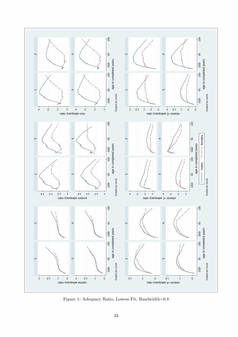
.511.52 .511.52

1018

5010

010

1850

100

12

34

calorie adequacy ratio

age

in c

ompl

eted

yea

rsG

raph

s by

rou

nd

11.21.41.6 11.21.41.6

1018

5010

010

1850

100

12

34

protein adequacy ratio

age

in c

ompl

eted

yea

rsG

raph

s by

rou

nd

.1.2.3.4 .1.2.3.4

1018

5010

010

1850

100

12

34

iron adequacy ratio

age

in c

ompl

eted

yea

rsG

raph

s by

rou

nd

.511.5 .511.5

1018

5010

010

1850

100

12

34

vitamin−A adequacy ratio

age

in c

ompl

eted

yea

rsG

raph

s by

rou

nd

1234 1234

1018

5010

010

1850

100

12

34

mal

esfe

mal

es

vitamin−C adequacy ratio

age

in c

ompl

eted

yea

rs

Gra

phs

by r

ound

0.511.52 0.511.52

1018

5010

010

1850

100

12

34

vitamin−D adequacy ratio

age

in c

ompl

eted

yea

rsG

raph

s by

rou

nd

Figure 1: Adequacy Ratio, Lowess Fit, Bandwidth=0.8

33

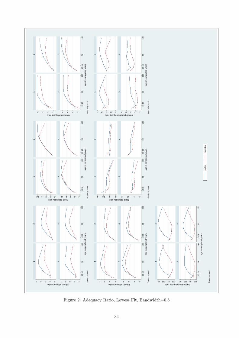
.2.4.6.81 .2.4.6.81

1018

5010

010

1850

100

12

34

calcium adequacy ratio

age

in c

ompl

eted

yea

rsG

raph

s by

rou

nd

.4.6.811.2 .4.6.811.2

1018

5010

010

1850

100

12

34

niacin adequacy ratio

age

in c

ompl

eted

yea

rsG

raph

s by

rou

nd

.3.4.5.6 .3.4.5.6

1018

5010

010

1850

100

12

34

riboflavin adequacy ratio

age

in c

ompl

eted

yea

rsG

raph

s by

rou

nd

.4.6.81 .4.6.81

1018

5010

010

1850

100

12

34

thiamin adequacy ratio

age

in c

ompl

eted

yea

rsG

raph

s by

rou

nd

.511.52 .511.5210

1850

100

1018

5010

0

12

34

folate adequacy ratio

age

in c

ompl

eted

yea

rsG

raph

s by

rou

nd

.1.15.2.25.3 .1.15.2.25.3

1018

5010

010

1850

100

12

34

animal−protein adequacy ratio

age

in c

ompl

eted

yea

rsG

raph

s by

rou

nd

.005.01.015.02 .005.01.015.02

1018

5010

010

1850

100

12

34

mal

esfe

mal

es

haem−iron adequacy ratio

age

in c

ompl

eted

yea

rs

Gra

phs

by r

ound

Figure 2: Adequacy Ratio, Lowess Fit, Bandwidth=0.8

34

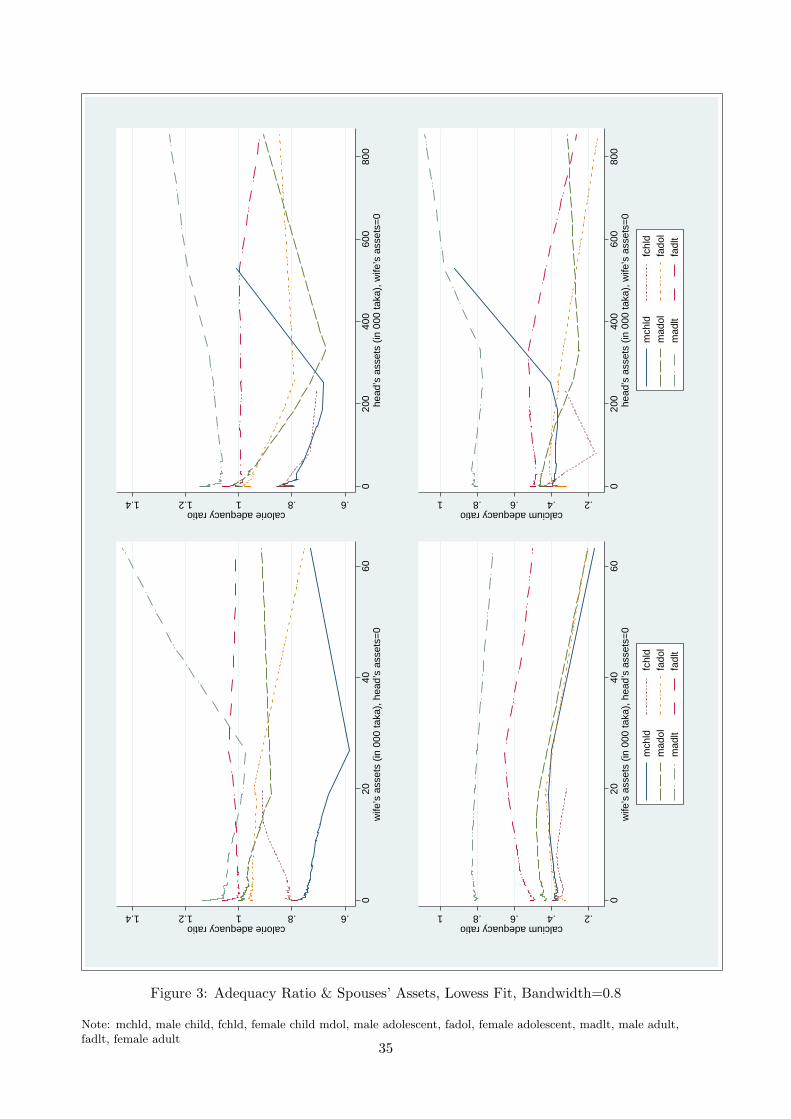
.6.811.21.4calorie adequacy ratio

020

4060

wife

’s a

sset

s (in

000

taka

), h

ead’

s as

sets

=0

.6.811.21.4calorie adequacy ratio

020

040

060

080

0he

ad’s

ass

ets

(in 0

00 ta

ka),

wife

’s a

sset

s=0

.2.4.6.81calcium adequacy ratio

020

4060

wife

’s a

sset

s (in

000

taka

), h

ead’

s as

sets

=0

mch

ldfc

hld

mad

olfa

dol

mad

ltfa

dlt

.2.4.6.81calcium adequacy ratio

020

040

060

080

0he

ad’s

ass

ets

(in 0

00 ta

ka),

wife

’s a

sset

s=0

mch

ldfc

hld

mad

olfa

dol

mad

ltfa

dlt

Figure 3: Adequacy Ratio & Spouses’ Assets, Lowess Fit, Bandwidth=0.8

Note: mchld, male child, fchld, female child mdol, male adolescent, fadol, female adolescent, madlt, male adult,fadlt, female adult

35

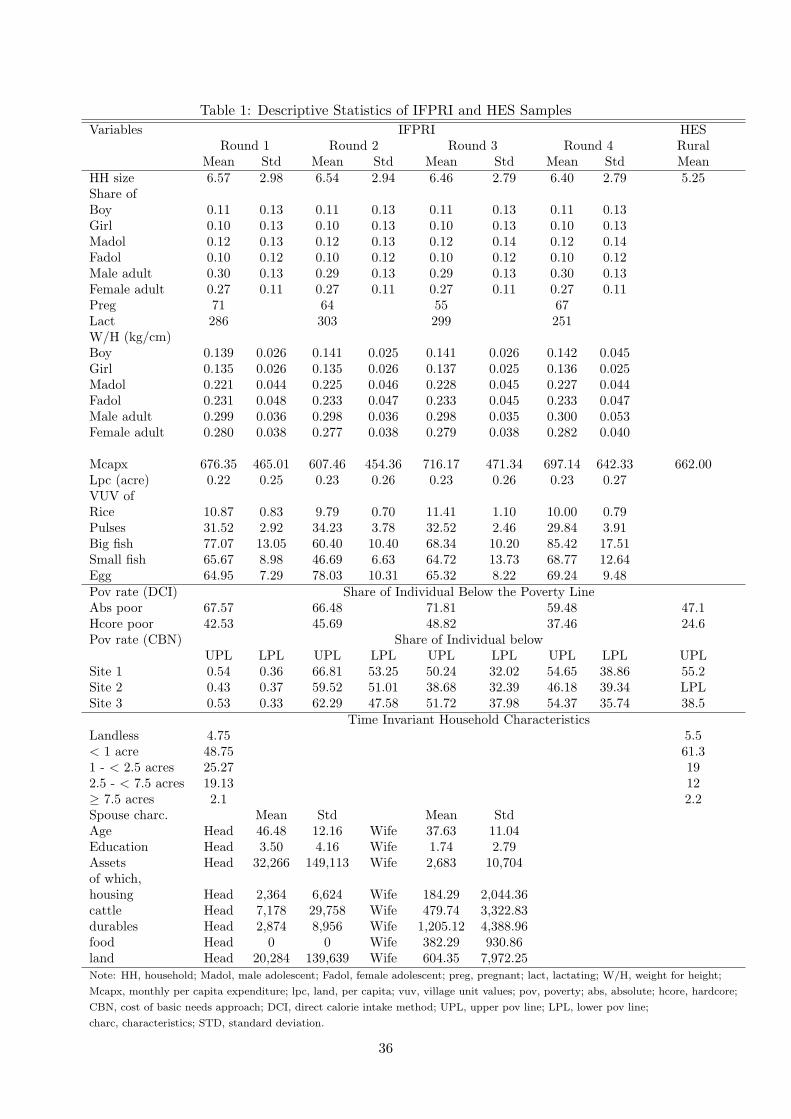
Table 1: Descriptive Statistics of IFPRI and HES Samples

Variables IFPRI HESRound 1 Round 2 Round 3 Round 4 Rural

Mean Std Mean Std Mean Std Mean Std MeanHH size 6.57 2.98 6.54 2.94 6.46 2.79 6.40 2.79 5.25Share ofBoy 0.11 0.13 0.11 0.13 0.11 0.13 0.11 0.13Girl 0.10 0.13 0.10 0.13 0.10 0.13 0.10 0.13Madol 0.12 0.13 0.12 0.13 0.12 0.14 0.12 0.14Fadol 0.10 0.12 0.10 0.12 0.10 0.12 0.10 0.12Male adult 0.30 0.13 0.29 0.13 0.29 0.13 0.30 0.13Female adult 0.27 0.11 0.27 0.11 0.27 0.11 0.27 0.11Preg 71 64 55 67Lact 286 303 299 251W/H (kg/cm)Boy 0.139 0.026 0.141 0.025 0.141 0.026 0.142 0.045Girl 0.135 0.026 0.135 0.026 0.137 0.025 0.136 0.025Madol 0.221 0.044 0.225 0.046 0.228 0.045 0.227 0.044Fadol 0.231 0.048 0.233 0.047 0.233 0.045 0.233 0.047Male adult 0.299 0.036 0.298 0.036 0.298 0.035 0.300 0.053Female adult 0.280 0.038 0.277 0.038 0.279 0.038 0.282 0.040

Mcapx 676.35 465.01 607.46 454.36 716.17 471.34 697.14 642.33 662.00Lpc (acre) 0.22 0.25 0.23 0.26 0.23 0.26 0.23 0.27VUV ofRice 10.87 0.83 9.79 0.70 11.41 1.10 10.00 0.79Pulses 31.52 2.92 34.23 3.78 32.52 2.46 29.84 3.91Big fish 77.07 13.05 60.40 10.40 68.34 10.20 85.42 17.51Small fish 65.67 8.98 46.69 6.63 64.72 13.73 68.77 12.64Egg 64.95 7.29 78.03 10.31 65.32 8.22 69.24 9.48Pov rate (DCI) Share of Individual Below the Poverty LineAbs poor 67.57 66.48 71.81 59.48 47.1Hcore poor 42.53 45.69 48.82 37.46 24.6Pov rate (CBN) Share of Individual below

UPL LPL UPL LPL UPL LPL UPL LPL UPLSite 1 0.54 0.36 66.81 53.25 50.24 32.02 54.65 38.86 55.2Site 2 0.43 0.37 59.52 51.01 38.68 32.39 46.18 39.34 LPLSite 3 0.53 0.33 62.29 47.58 51.72 37.98 54.37 35.74 38.5

Time Invariant Household CharacteristicsLandless 4.75 5.5< 1 acre 48.75 61.31 - < 2.5 acres 25.27 192.5 - < 7.5 acres 19.13 12≥ 7.5 acres 2.1 2.2Spouse charc. Mean Std Mean StdAge Head 46.48 12.16 Wife 37.63 11.04Education Head 3.50 4.16 Wife 1.74 2.79Assets Head 32,266 149,113 Wife 2,683 10,704of which,housing Head 2,364 6,624 Wife 184.29 2,044.36cattle Head 7,178 29,758 Wife 479.74 3,322.83durables Head 2,874 8,956 Wife 1,205.12 4,388.96food Head 0 0 Wife 382.29 930.86land Head 20,284 139,639 Wife 604.35 7,972.25Note: HH, household; Madol, male adolescent; Fadol, female adolescent; preg, pregnant; lact, lactating; W/H, weight for height;

Mcapx, monthly per capita expenditure; lpc, land, per capita; vuv, village unit values; pov, poverty; abs, absolute; hcore, hardcore;

CBN, cost of basic needs approach; DCI, direct calorie intake method; UPL, upper pov line; LPL, lower pov line;

charc, characteristics; STD, standard deviation.

36

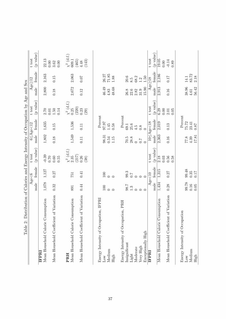
Tab

le2:

Distribution

ofCaloriesan

dEnergy

Intensity

ofOccupationbyAgeandSex

Age<6

ttest

6≤Age<12

ttest

Age≥12

ttest

male

female

(pvalue)

male

female

(pvalue)

male

female

(pvalue)

IFPRI

MeanHou

seholdCalorie

Con

sumption

1,07

81,12

7-0.39

1,80

21,63

52.70

2,80

02,16

322

.13

0.70

0.01

0.00

MeanHou

seholdCoeffi

cientof

Variation

0.32

0.27

0.60

0.18

0.15

1.50

0.18

0.15

3.62

0.55

0.14

0.00

PRH

χ2(d.f.)

χ2(d.f.)

χ2(d.f.)

MeanHou

seholdCalorie

Con

sumption

891

751

2.35

1,54

91,53

60.25

2,67

22,06

360

9.1

(217

)(220

)(465

)MeanHou

seholdCoeffi

cientof

Variation

0.44

0.41

0.26

0.11

0.11

0.23

0.12

0.07

4.48

(38)

(29)

(143

)

Energy

Intensity

ofOccupation

,IF

PRI

Percent

Low

100

100

98.31

97.97

46.49

26.27

Medium

00

0.54

1.45

4.83

71.85

High

00

1.15

0.58

48.68

1.88

EnergyIntensity

ofOccupation,PRH

Percent

Insign

ificant

98.7

99.3

70.5

69.1

26.8

20.6

Light

1.3

0.7

28.8

25.6

22.6

8.5

Moderate

00

04.5

2.82

68.2

VeryHigh

00

0.7

0.8

31.9

1.2

Exception

ally

High

00

00

15.90

1.50

IFPRI

Age<10

ttest

10≤Age<18

ttest

Age≥18

ttest

male

female

(pvalue)

male

female

(pvalue)

male

female

(pvalue)

MeanHou

seholdCalorie

Con

sumption

1,43

41,31

52.18

2,36

32,019

6.29

2,91

32,18

619

.05

0.03

0.00

0.00

MeanHou

seholdCoeffi

cientof

Variation

0.28

0.27

0.56

0.16

0.13

2.01

0.16

0.17

-0.14

0.58

0.05

0.89

Energy

Intensity

ofOccupation

Percent

Low

99.78

99.48

77.8

75.72

38.96

14.1

Medium

0.16

0.35

4.39

23.41

4.61

83.72

High

0.05

0.17

17.81

0.87

56.42

2.18

37

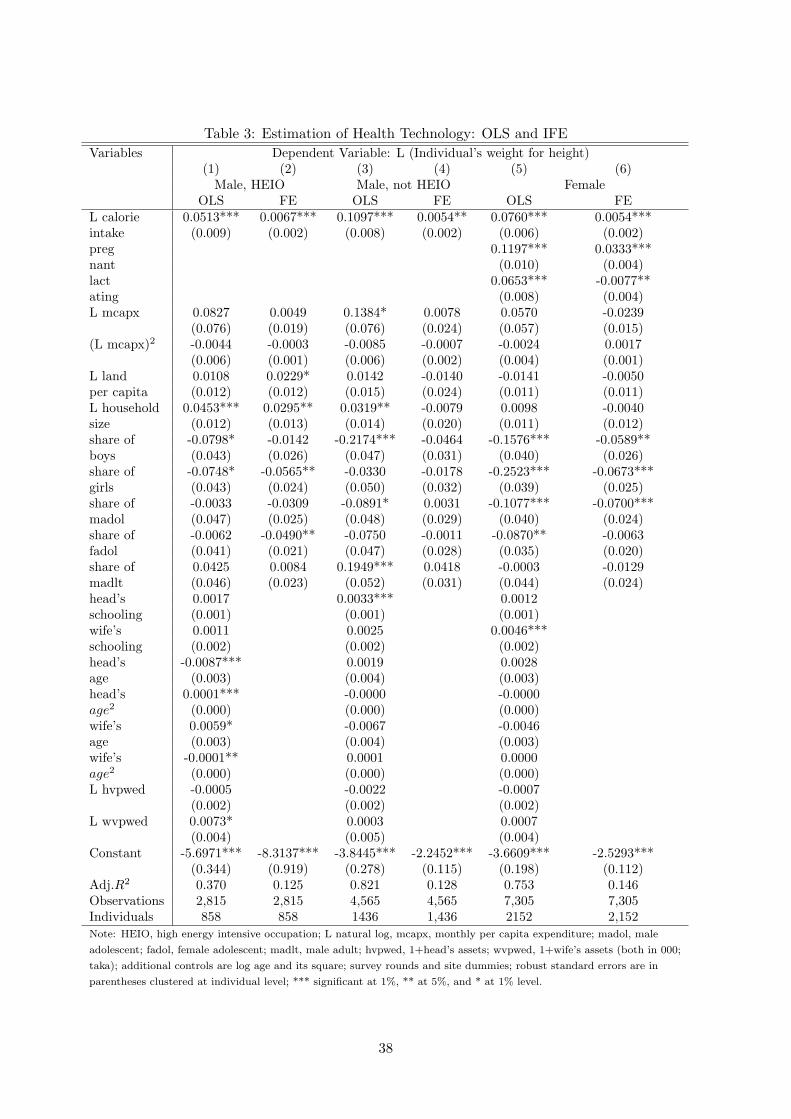
Table 3: Estimation of Health Technology: OLS and IFE

Variables Dependent Variable: L (Individual’s weight for height)(1) (2) (3) (4) (5) (6)Male, HEIO Male, not HEIO Female

OLS FE OLS FE OLS FEL calorie 0.0513*** 0.0067*** 0.1097*** 0.0054** 0.0760*** 0.0054***intake (0.009) (0.002) (0.008) (0.002) (0.006) (0.002)preg 0.1197*** 0.0333***nant (0.010) (0.004)lact 0.0653*** -0.0077**ating (0.008) (0.004)L mcapx 0.0827 0.0049 0.1384* 0.0078 0.0570 -0.0239

(0.076) (0.019) (0.076) (0.024) (0.057) (0.015)(L mcapx)2 -0.0044 -0.0003 -0.0085 -0.0007 -0.0024 0.0017

(0.006) (0.001) (0.006) (0.002) (0.004) (0.001)L land 0.0108 0.0229* 0.0142 -0.0140 -0.0141 -0.0050per capita (0.012) (0.012) (0.015) (0.024) (0.011) (0.011)L household 0.0453*** 0.0295** 0.0319** -0.0079 0.0098 -0.0040size (0.012) (0.013) (0.014) (0.020) (0.011) (0.012)share of -0.0798* -0.0142 -0.2174*** -0.0464 -0.1576*** -0.0589**boys (0.043) (0.026) (0.047) (0.031) (0.040) (0.026)share of -0.0748* -0.0565** -0.0330 -0.0178 -0.2523*** -0.0673***girls (0.043) (0.024) (0.050) (0.032) (0.039) (0.025)share of -0.0033 -0.0309 -0.0891* 0.0031 -0.1077*** -0.0700***madol (0.047) (0.025) (0.048) (0.029) (0.040) (0.024)share of -0.0062 -0.0490** -0.0750 -0.0011 -0.0870** -0.0063fadol (0.041) (0.021) (0.047) (0.028) (0.035) (0.020)share of 0.0425 0.0084 0.1949*** 0.0418 -0.0003 -0.0129madlt (0.046) (0.023) (0.052) (0.031) (0.044) (0.024)head’s 0.0017 0.0033*** 0.0012schooling (0.001) (0.001) (0.001)wife’s 0.0011 0.0025 0.0046***schooling (0.002) (0.002) (0.002)head’s -0.0087*** 0.0019 0.0028age (0.003) (0.004) (0.003)head’s 0.0001*** -0.0000 -0.0000age2 (0.000) (0.000) (0.000)wife’s 0.0059* -0.0067 -0.0046age (0.003) (0.004) (0.003)wife’s -0.0001** 0.0001 0.0000age2 (0.000) (0.000) (0.000)L hvpwed -0.0005 -0.0022 -0.0007

(0.002) (0.002) (0.002)L wvpwed 0.0073* 0.0003 0.0007

(0.004) (0.005) (0.004)Constant -5.6971*** -8.3137*** -3.8445*** -2.2452*** -3.6609*** -2.5293***

(0.344) (0.919) (0.278) (0.115) (0.198) (0.112)Adj.R2 0.370 0.125 0.821 0.128 0.753 0.146Observations 2,815 2,815 4,565 4,565 7,305 7,305Individuals 858 858 1436 1,436 2152 2,152Note: HEIO, high energy intensive occupation; L natural log, mcapx, monthly per capita expenditure; madol, male

adolescent; fadol, female adolescent; madlt, male adult; hvpwed, 1+head’s assets; wvpwed, 1+wife’s assets (both in 000;

taka); additional controls are log age and its square; survey rounds and site dummies; robust standard errors are in

parentheses clustered at individual level; *** significant at 1%, ** at 5%, and * at 1% level.

38

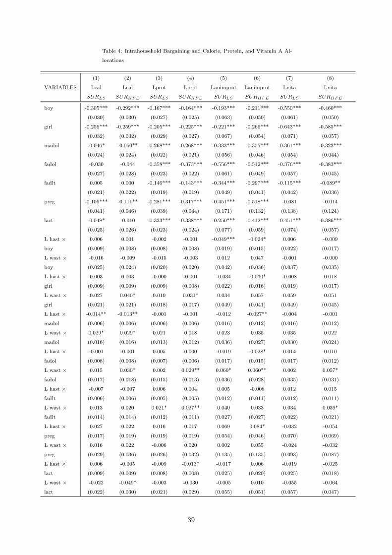
Table 4: Intrahousehold Bargaining and Calorie, Protein, and Vitamin A Al-

locations

(1) (2) (3) (4) (5) (6) (7) (8)

VARIABLES Lcal Lcal Lprot Lprot Lanimprot Lanimprot Lvita Lvita

SURLS SURHFE SURLS SURHFE SURLS SURHFE SURLS SURHFE

boy -0.305*** -0.292*** -0.167*** -0.164*** -0.193*** -0.211*** -0.550*** -0.460***

(0.030) (0.030) (0.027) (0.025) (0.063) (0.050) (0.061) (0.050)

girl -0.256*** -0.259*** -0.205*** -0.225*** -0.221*** -0.266*** -0.643*** -0.585***

(0.032) (0.032) (0.029) (0.027) (0.067) (0.054) (0.071) (0.057)

madol -0.046* -0.050** -0.268*** -0.268*** -0.333*** -0.355*** -0.361*** -0.322***

(0.024) (0.024) (0.022) (0.021) (0.056) (0.046) (0.054) (0.044)

fadol -0.030 -0.044 -0.358*** -0.373*** -0.556*** -0.512*** -0.376*** -0.383***

(0.027) (0.028) (0.023) (0.022) (0.061) (0.049) (0.057) (0.045)

fadlt 0.005 0.000 -0.146*** -0.143*** -0.344*** -0.297*** -0.115*** -0.089**

(0.021) (0.022) (0.019) (0.019) (0.049) (0.041) (0.042) (0.036)

preg -0.106*** -0.111** -0.281*** -0.317*** -0.451*** -0.518*** -0.081 -0.014

(0.041) (0.046) (0.039) (0.044) (0.171) (0.132) (0.138) (0.124)

lact -0.048* -0.010 -0.333*** -0.338*** -0.250*** -0.412*** -0.451*** -0.386***

(0.025) (0.026) (0.023) (0.024) (0.077) (0.059) (0.074) (0.057)

L hast × 0.006 0.001 -0.002 -0.001 -0.049*** -0.024* 0.006 -0.009

boy (0.009) (0.008) (0.008) (0.008) (0.019) (0.015) (0.022) (0.017)

L wast × -0.016 -0.009 -0.015 -0.003 0.012 0.047 -0.001 -0.000

boy (0.025) (0.024) (0.020) (0.020) (0.042) (0.036) (0.037) (0.035)

L hast × 0.003 0.003 -0.000 -0.001 -0.034 -0.030* -0.008 0.018

girl (0.009) (0.009) (0.009) (0.008) (0.022) (0.016) (0.019) (0.017)

L wast × 0.027 0.040* 0.010 0.031* 0.034 0.057 0.059 0.051

girl (0.021) (0.021) (0.018) (0.017) (0.049) (0.041) (0.049) (0.045)

L hast × -0.014** -0.013** -0.001 -0.001 -0.012 -0.027** -0.004 -0.001

madol (0.006) (0.006) (0.006) (0.006) (0.016) (0.012) (0.016) (0.012)

L wast × 0.029* 0.029* 0.021 0.018 0.023 0.035 0.035 0.022

madol (0.016) (0.016) (0.013) (0.012) (0.036) (0.027) (0.030) (0.024)

L hast × -0.001 -0.001 0.005 0.000 -0.019 -0.028* 0.014 0.010

fadol (0.008) (0.008) (0.007) (0.006) (0.017) (0.015) (0.017) (0.012)

L wast × 0.015 0.030* 0.002 0.029** 0.060* 0.060** 0.002 0.057*

fadol (0.017) (0.018) (0.015) (0.013) (0.036) (0.028) (0.035) (0.031)

L hast × -0.007 -0.007 0.006 0.004 0.005 -0.008 0.012 0.015

fadlt (0.006) (0.006) (0.005) (0.005) (0.012) (0.011) (0.012) (0.011)

L wast × 0.013 0.020 0.021* 0.027** 0.040 0.033 0.034 0.039*

fadlt (0.014) (0.014) (0.012) (0.011) (0.027) (0.027) (0.022) (0.021)

L hast × 0.027 0.022 0.016 0.017 0.069 0.084* -0.032 -0.054

preg (0.017) (0.019) (0.019) (0.019) (0.054) (0.046) (0.070) (0.069)

L wast × 0.016 0.022 -0.006 0.020 0.002 0.055 -0.024 -0.032

preg (0.029) (0.036) (0.026) (0.032) (0.135) (0.135) (0.093) (0.087)

L hast × 0.006 -0.005 -0.009 -0.013* -0.017 0.006 -0.019 -0.025

lact (0.009) (0.009) (0.008) (0.008) (0.025) (0.020) (0.025) (0.018)

L wast × -0.022 -0.049* -0.003 -0.030 -0.005 0.010 -0.055 -0.064

lact (0.022) (0.030) (0.021) (0.029) (0.055) (0.051) (0.057) (0.047)

39

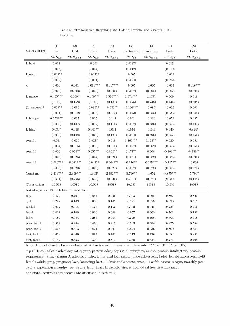
Table 4: Intrahousehold Bargaining and Calorie, Protein, and Vitamin A Al-

locations

(1) (2) (3) (4) (5) (6) (7) (8)

VARIABLES Lcal Lcal Lprot Lprot Lanimprot Lanimprot Lvita Lvita

SURLS SURHFE SURLS SURHFE SURLS SURHFE SURLS SURHFE

L hast 0.001 -0.001 0.023** 0.015

(0.005) (0.004) (0.012) (0.010)

L wast -0.028** -0.022** -0.007 -0.014

(0.012) (0.011) (0.024) (0.022)

κ 0.000 0.001 -0.019*** -0.017*** -0.005 -0.005 -0.004 -0.016***

(0.003) (0.003) (0.003) (0.002) (0.007) (0.005) (0.007) (0.005)

L mcapx 0.435*** 0.300* 0.478*** 0.526*** 2.074*** 1.405* 0.509 0.019

(0.152) (0.168) (0.168) (0.181) (0.575) (0.748) (0.444) (0.608)

(L macapx)2 -0.026** -0.016 -0.030** -0.032** -0.126*** -0.089 -0.032 0.003

(0.011) (0.012) (0.013) (0.013) (0.043) (0.055) (0.033) (0.045)

L landpc 0.052*** -0.067 0.025 -0.142 0.021 -0.236 -0.072 0.457

(0.018) (0.107) (0.017) (0.113) (0.057) (0.436) (0.055) (0.407)

L hhsz 0.030* 0.048 0.041** -0.032 0.074 -0.249 0.049 0.824*

(0.018) (0.108) (0.020) (0.121) (0.064) (0.496) (0.057) (0.452)

round1 -0.021 -0.020 0.027* 0.019 0.166*** 0.123** 0.020 0.051

(0.014) (0.015) (0.015) (0.015) (0.057) (0.062) (0.056) (0.060)

round2 0.036 0.054** 0.057** 0.062** 0.177** 0.008 -0.206** -0.239**

(0.023) (0.025) (0.024) (0.026) (0.081) (0.089) (0.085) (0.095)

round3 -0.080*** -0.083*** -0.045** -0.064*** -0.146** -0.215*** -0.137** -0.098

(0.018) (0.020) (0.020) (0.021) (0.067) (0.079) (0.065) (0.075)

Constant -2.413*** -2.309*** -1.303* -2.192*** -5.716** -4.652 -5.875*** -5.709*

(0.611) (0.766) (0.673) (0.832) (2.481) (3.571) (2.030) (3.148)

Observations 10,555 10515 10,555 10515 10,555 10515 10,555 10515

test of equation 13 for L hast=L wast, for :

boy 0.429 0.701 0.557 0.956 0.193 0.065 0.867 0.820

girl 0.282 0.103 0.610 0.103 0.221 0.059 0.220 0.513

madol 0.012 0.015 0.123 0.152 0.402 0.045 0.235 0.416

fadol 0.412 0.108 0.886 0.046 0.057 0.009 0.761 0.150

fadlt 0.189 0.084 0.283 0.064 0.279 0.196 0.404 0.318

preg, fadol 0.902 0.484 0.490 0.419 0.933 0.684 0.975 0.554

preg, fadlt 0.806 0.513 0.821 0.491 0.824 0.936 0.800 0.681

lact, fadol 0.679 0.669 0.894 0.702 0.213 0.126 0.482 0.881

lact, fadlt 0.742 0.533 0.370 0.813 0.350 0.324 0.771 0.705

Note: Robust standard errors clustered at the household level are in brackets. *** p<0.01, ** p<0.05,

* p<0.1; cal, calorie adequacy ratio; prot, protein adequacy ratio; animprot, animal protein intake/total protein

requirement; vita, vitamin A adequacy ratio; L, natural log; madol, male adolescent; fadol, female adolescent; fadlt,

female adult; preg, pregnant; lact, lactating; hast, 1+husband’s assets; wast, 1+wife’s assets; mcapx, monthly per

capita expenditure; landpc, per capita land; hhsz, household size; κ, individual health endowment;

additional controls (not shown) are discussed in section 4.

40

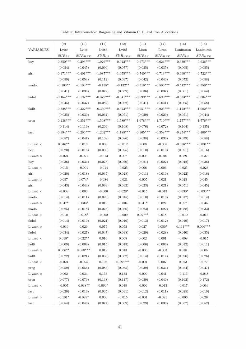
Table 5: Intrahousehold Bargaining and Vitamin C, D, and Iron Allocations

(9) (10) (11) (12) (13) (14) (15) (16)

VARIABLES Lvitc Lvitc Lvitd Lvitd Liron Liron Lanimiron Lanimiron

SURLS SURHFE SURLS SURHFE SURLS SURHFE SURLS SURHFE

boy -0.350*** -0.293*** -1.026*** -0.942*** -0.673*** -0.624*** -0.630*** -0.636***

(0.054) (0.045) (0.096) (0.077) (0.035) (0.035) (0.065) (0.055)

girl -0.471*** -0.401*** -1.087*** -1.055*** -0.740*** -0.713*** -0.690*** -0.722***

(0.059) (0.054) (0.112) (0.097) (0.042) (0.040) (0.072) (0.058)

madol -0.103** -0.103*** -0.135* -0.132** -0.516*** -0.506*** -0.512*** -0.559***

(0.041) (0.036) (0.072) (0.059) (0.036) (0.037) (0.061) (0.054)

fadol -0.164*** -0.197*** -0.379*** -0.341*** -0.699*** -0.690*** -0.833*** -0.804***

(0.045) (0.037) (0.082) (0.062) (0.041) (0.041) (0.065) (0.058)

fadlt -0.328*** -0.322*** -0.350*** -0.323*** -0.951*** -0.925*** -1.122*** -1.082***

(0.035) (0.030) (0.064) (0.051) (0.029) (0.029) (0.051) (0.044)

preg -0.438*** -0.351*** -1.598*** -1.589*** -1.678*** -1.710*** -1.777*** -1.776***

(0.114) (0.119) (0.209) (0.168) (0.076) (0.072) (0.164) (0.135)

lact -0.394*** -0.296*** -1.202*** -1.188*** -0.365*** -0.358*** -0.254*** -0.409***

(0.057) (0.047) (0.108) (0.086) (0.038) (0.036) (0.079) (0.058)

L hast × 0.046** 0.018 0.008 -0.012 0.008 -0.005 -0.056*** -0.031**

boy (0.020) (0.015) (0.030) (0.025) (0.010) (0.010) (0.021) (0.016)

L wast × -0.024 -0.021 -0.013 0.007 -0.005 -0.010 0.039 0.037

boy (0.036) (0.034) (0.078) (0.070) (0.021) (0.022) (0.042) (0.036)

L hast × 0.015 -0.001 -0.014 -0.025 0.006 0.006 -0.025 -0.023

girl (0.020) (0.018) (0.035) (0.028) (0.011) (0.010) (0.022) (0.016)

L wast × 0.057 0.074* -0.084 -0.021 -0.005 0.021 0.025 0.045

girl (0.043) (0.044) (0.093) (0.092) (0.023) (0.021) (0.051) (0.045)

L hast × -0.009 0.003 -0.006 -0.028* -0.015 -0.013 -0.030* -0.033**

madol (0.014) (0.011) (0.020) (0.015) (0.010) (0.010) (0.017) (0.014)

L wast × 0.047* 0.033* 0.019 -0.004 0.041* 0.024 0.027 0.045

madol (0.025) (0.018) (0.046) (0.036) (0.023) (0.022) (0.038) (0.033)

L hast × 0.010 0.018* -0.002 -0.009 0.027** 0.018 -0.010 -0.015

fadol (0.014) (0.010) (0.021) (0.016) (0.013) (0.012) (0.019) (0.017)

L wast × -0.039 0.029 0.075 0.053 0.027 0.050* 0.111*** 0.096***

fadol (0.034) (0.027) (0.047) (0.038) (0.029) (0.028) (0.040) (0.035)

L hast × 0.018* 0.022** 0.010 0.008 0.002 0.001 -0.008 -0.015

fadlt (0.009) (0.009) (0.015) (0.013) (0.006) (0.006) (0.012) (0.011)

L wast × 0.056** 0.058*** 0.012 0.013 -0.006 -0.003 0.018 0.005

fadlt (0.022) (0.021) (0.033) (0.032) (0.014) (0.014) (0.026) (0.026)

L hast × -0.024 -0.025 0.106 0.186*** -0.001 0.007 0.073 0.077

preg (0.059) (0.056) (0.085) (0.065) (0.039) (0.034) (0.054) (0.047)

L wast × 0.062 0.034 0.153 0.132 -0.009 0.041 -0.115 -0.048

preg (0.077) (0.079) (0.138) (0.117) (0.039) (0.040) (0.162) (0.172)

L hast × -0.007 -0.038** 0.060* 0.019 -0.006 -0.013 -0.017 0.004

lact (0.020) (0.016) (0.035) (0.031) (0.012) (0.011) (0.025) (0.019)

L wast × -0.101* -0.089* 0.000 -0.015 -0.001 -0.021 -0.006 0.026

lact (0.054) (0.048) (0.077) (0.069) (0.029) (0.038) (0.057) (0.052)

41

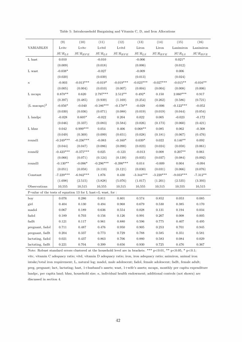
Table 5: Intrahousehold Bargaining and Vitamin C, D, and Iron Allocations

(9) (10) (11) (12) (13) (14) (15) (16)

VARIABLES Lvitc Lvitc Lvitd Lvitd Liron Liron Lanimiron Lanimiron

SURLS SURHFE SURLS SURHFE SURLS SURHFE SURLS SURHFE

L hast 0.010 -0.010 -0.006 0.021*

(0.009) (0.018) (0.006) (0.012)

L wast -0.038* -0.027 -0.009 0.006

(0.020) (0.039) (0.013) (0.024)

κ -0.003 -0.013*** -0.019* -0.019*** -0.023*** -0.027*** -0.015** -0.016**

(0.005) (0.004) (0.010) (0.007) (0.004) (0.004) (0.008) (0.006)

L mcapx 0.878** 0.620 2.797*** 2.512** 0.492* 0.150 2.060*** 0.917

(0.397) (0.485) (0.939) (1.169) (0.254) (0.262) (0.586) (0.721)

(L macapx)2 -0.056* -0.040 -0.186*** -0.178** -0.029 -0.006 -0.122*** -0.052

(0.030) (0.036) (0.071) (0.088) (0.019) (0.019) (0.044) (0.054)

L landpc -0.028 0.605* -0.022 0.204 0.022 0.005 -0.023 -0.172

(0.046) (0.337) (0.083) (0.584) (0.026) (0.173) (0.060) (0.421)

L hhsz 0.042 0.999*** 0.054 0.406 0.068** 0.085 0.062 -0.308

(0.049) (0.369) (0.099) (0.651) (0.028) (0.181) (0.067) (0.476)

round1 -0.249*** -0.236*** -0.083 -0.160* 0.039* 0.022 0.146** 0.092

(0.044) (0.047) (0.086) (0.090) (0.023) (0.024) (0.058) (0.061)

round2 -0.423*** -0.375*** 0.025 -0.123 -0.013 0.008 0.207** 0.061

(0.066) (0.071) (0.124) (0.139) (0.035) (0.037) (0.084) (0.092)

round3 -0.130** -0.096* -0.296*** -0.390*** 0.014 -0.009 0.004 -0.094

(0.051) (0.058) (0.110) (0.121) (0.030) (0.031) (0.066) (0.076)

Constant -7.229*** -6.942*** 1.876 0.430 -3.344*** -3.220*** -9.033*** -7.312**

(1.698) (2.515) (3.828) (5.076) (1.017) (1.201) (2.535) (3.393)

Observations 10,555 10,515 10,555 10,515 10,555 10,515 10,555 10,515

P-value of the tests of equation 13 for L hast=L wast, for :

boy 0.076 0.286 0.811 0.801 0.574 0.852 0.053 0.085

girl 0.404 0.130 0.494 0.968 0.679 0.530 0.385 0.170

madol 0.067 0.189 0.636 0.554 0.028 0.131 0.194 0.034

fadol 0.189 0.703 0.156 0.126 0.991 0.267 0.008 0.005

fadlt 0.121 0.117 0.961 0.880 0.596 0.775 0.407 0.495

pregnant, fadol 0.711 0.487 0.476 0.950 0.905 0.253 0.701 0.945

pregnant, fadlt 0.204 0.337 0.773 0.729 0.788 0.585 0.351 0.581

lactating, fadol 0.021 0.437 0.863 0.706 0.880 0.583 0.084 0.029

lactating, fadlt 0.221 0.704 0.399 0.656 0.930 0.725 0.476 0.367

Note: Robust standard errors clustered at the household level are in brackets. *** p<0.01, ** p<0.05, * p<0.1;

vitc, vitamin C adequacy ratio; vitd, vitamin D adequacy ratio; iron, iron adequacy ratio; animiron, animal iron

intake/total iron requirement; L, natural log; madol, male adolescent; fadol, female adolescent; fadlt, female adult;

preg, pregnant; lact, lactating; hast, 1+husband’s assets; wast, 1+wife’s assets; mcapx, monthly per capita expenditure

landpc, per capita land; hhsz, household size; κ, individual health endowment; additional controls (not shown) are

discussed in section 4.

42

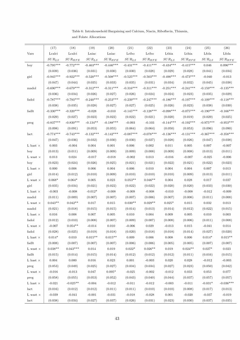
Table 6: Intrahousehold Bargaining and Calcium, Niacin, Riboflavin, Thiamin,

and Folate Allocations

(17) (18) (19) (20) (21) (22) (23) (24) (25) (26)

Vars Lcalci Lcalci Lniac Lniac Lribo Lribo Lthia Lthia Lfola Lfola

SURLS SURHFE SURLS SURHFE SURLS SURHFE SURLS SURHFE SURLS SURHFE

boy -0.795*** -0.772*** -0.463*** -0.446*** -0.431*** -0.411*** -0.434*** -0.415*** 0.046 0.096***

(0.039) (0.036) (0.031) (0.030) (0.030) (0.028) (0.029) (0.028) (0.041) (0.034)

girl -0.945*** -0.922*** -0.520*** -0.508*** -0.525*** -0.503*** -0.490*** -0.473*** -0.040 -0.013

(0.047) (0.044) (0.035) (0.033) (0.035) (0.031) (0.034) (0.032) (0.045) (0.038)

madol -0.690*** -0.679*** -0.312*** -0.311*** -0.316*** -0.311*** -0.251*** -0.241*** -0.159*** -0.135***

(0.036) (0.034) (0.026) (0.027) (0.026) (0.024) (0.024) (0.023) (0.035) (0.029)

fadol -0.787*** -0.793*** -0.240*** -0.253*** -0.239*** -0.247*** -0.186*** -0.197*** -0.109*** -0.118***

(0.038) (0.035) (0.028) (0.027) (0.027) (0.025) (0.026) (0.023) (0.038) (0.030)

fadlt -0.330*** -0.320*** -0.028 -0.010 -0.145*** -0.128*** -0.098*** -0.075*** -0.190*** -0.166***

(0.029) (0.027) (0.023) (0.022) (0.022) (0.021) (0.020) (0.019) (0.029) (0.025)

preg -0.837*** -0.830*** -0.134** -0.188*** -0.093 -0.103 -0.144*** -0.192*** -0.975*** -0.953***

(0.098) (0.091) (0.053) (0.055) (0.064) (0.064) (0.050) (0.053) (0.096) (0.090)

lact -0.774*** -0.743*** -0.132*** -0.142*** -0.087*** -0.078*** -0.136*** -0.131*** -0.367*** -0.358***

(0.047) (0.036) (0.032) (0.030) (0.030) (0.027) (0.028) (0.026) (0.047) (0.038)

L hast × 0.003 -0.004 0.004 0.001 0.006 0.002 0.011 0.005 0.007 -0.007

boy (0.013) (0.011) (0.009) (0.009) (0.009) (0.008) (0.009) (0.008) (0.013) (0.011)

L wast × 0.013 0.024 -0.017 -0.018 -0.002 0.013 -0.016 -0.007 -0.025 -0.006

boy (0.023) (0.024) (0.026) (0.025) (0.021) (0.021) (0.022) (0.021) (0.022) (0.023)

L hast × 0.000 0.008 0.006 0.004 0.006 0.010 0.004 0.004 0.007 0.013

girl (0.014) (0.012) (0.010) (0.009) (0.010) (0.010) (0.010) (0.009) (0.013) (0.011)

L wast × 0.068* 0.064* 0.005 0.023 0.053** 0.046** 0.004 0.028 0.017 0.037

girl (0.035) (0.034) (0.021) (0.022) (0.022) (0.022) (0.020) (0.020) (0.033) (0.030)

L hast × -0.003 -0.008 -0.012* -0.008 -0.009 -0.008 -0.010 -0.008 -0.012 -0.009

madol (0.011) (0.009) (0.007) (0.007) (0.007) (0.006) (0.007) (0.006) (0.011) (0.008)

L wast × 0.043** 0.042** 0.017 0.015 0.030** 0.029** 0.025* 0.015 0.032 0.013

madol (0.021) (0.018) (0.015) (0.015) (0.014) (0.013) (0.014) (0.012) (0.022) (0.015)

L hast × 0.016 0.008 0.007 0.005 0.010 0.004 0.009 0.005 0.010 0.003

fadol (0.012) (0.010) (0.008) (0.007) (0.009) (0.007) (0.008) (0.006) (0.011) (0.008)

L wast × -0.007 0.054** -0.014 0.010 -0.006 0.029 -0.013 0.015 -0.041 0.014

fadol (0.028) (0.025) (0.019) (0.018) (0.020) (0.018) (0.018) (0.014) (0.027) (0.020)

L hast × 0.014* 0.010 0.015** 0.015** 0.009 0.006 0.008 0.006 0.014* 0.015**

fadlt (0.008) (0.007) (0.007) (0.007) (0.006) (0.006) (0.005) (0.005) (0.007) (0.007)

L wast × 0.038** 0.043*** 0.014 0.019 0.022* 0.026** 0.019 0.024** 0.027* 0.023

fadlt (0.015) (0.014) (0.015) (0.014) (0.012) (0.012) (0.012) (0.011) (0.016) (0.015)

L hast × 0.004 0.000 0.016 0.023 0.001 -0.003 0.020 0.028 -0.012 -0.003

preg (0.053) (0.049) (0.025) (0.027) (0.034) (0.034) (0.027) (0.023) (0.050) (0.042)

L wast × -0.016 -0.013 0.047 0.095* -0.025 -0.002 -0.012 0.033 0.053 0.077

preg (0.058) (0.055) (0.053) (0.052) (0.043) (0.040) (0.044) (0.037) (0.057) (0.057)

L hast × -0.021 -0.025** -0.004 -0.012 -0.011 -0.012 -0.003 -0.011 -0.031* -0.036***

lact (0.016) (0.012) (0.012) (0.011) (0.011) (0.010) (0.010) (0.008) (0.017) (0.013)

L wast × -0.039 -0.041 -0.001 -0.031 -0.018 -0.028 0.001 -0.020 -0.037 -0.019

lact (0.038) (0.034) (0.027) (0.037) (0.026) (0.031) (0.023) (0.030) (0.037) (0.035)

43

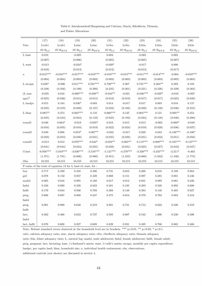
Table 6: Intrahousehold Bargaining and Calcium, Niacin, Riboflavin, Thiamin,

and Folate Allocations

(17) (18) (19) (20) (21) (22) (23) (24) (25) (26)

Vars Lcalci Lcalci Lniac Lniac Lribo Lribo Lthia Lthia Lfola Lfola

SURLS SURHFE SURLS SURHFE SURLS SURHFE SURLS SURHFE SURLS SURHFE

L hast 0.010 -0.005 0.004 -0.005 0.003

(0.007) (0.006) (0.005) (0.005) (0.007)

L wast -0.013 -0.024* -0.020* -0.017 0.000

(0.016) (0.013) (0.012) (0.013) (0.017)

κ -0.012*** -0.016*** -0.017*** -0.018*** -0.010*** -0.013*** -0.011*** -0.014*** -0.004 -0.010***

(0.004) (0.004) (0.003) (0.003) (0.003) (0.003) (0.003) (0.003) (0.005) (0.003)

L mcapx 0.638* -0.090 0.911*** 0.591*** 0.720*** 0.367 0.731*** 0.464** 0.393 0.183

(0.328) (0.356) (0.199) (0.209) (0.235) (0.261) (0.221) (0.226) (0.329) (0.382)

(L mac -0.035 0.016 -0.060*** -0.038** -0.044** -0.021 -0.046*** -0.029* -0.018 -0.007

apx)2 (0.025) (0.026) (0.015) (0.015) (0.018) (0.019) (0.017) (0.017) (0.025) (0.028)

L landpc 0.015 0.184 0.036* -0.001 0.014 -0.017 0.017 0.003 0.016 0.157

(0.035) (0.219) (0.020) (0.127) (0.022) (0.166) (0.020) (0.140) (0.036) (0.255)

L hhsz 0.085** 0.374 0.083*** 0.110 0.066*** 0.125 0.064*** 0.121 0.095** 0.254

(0.035) (0.244) (0.024) (0.133) (0.025) (0.192) (0.024) (0.148) (0.040) (0.280)

round1 0.046 0.064* -0.018 -0.035* 0.018 0.015 0.013 -0.003 -0.069* -0.049

(0.034) (0.035) (0.018) (0.019) (0.022) (0.024) (0.019) (0.020) (0.036) (0.037)

round2 0.049 0.008 0.053* 0.067** -0.022 -0.017 0.029 0.043 -0.136*** -0.106*

(0.050) (0.053) (0.030) (0.031) (0.035) (0.038) (0.031) (0.032) (0.051) (0.056)

round3 -0.013 0.012 0.070*** 0.042* -0.058** -0.065** 0.113*** 0.089*** -0.165*** -0.127***

(0.041) (0.044) (0.024) (0.025) (0.028) (0.031) (0.025) (0.027) (0.043) (0.047)

Const. -6.956*** -5.018*** -3.636*** -3.516*** -5.121*** -4.479*** -3.328*** -3.245*** -2.211* -0.463

(1.371) (1.781) (0.806) (0.980) (0.951) (1.253) (0.860) (1.032) (1.340) (1.773)

Obs. 10,555 10,515 10,555 10,515 10,555 10,515 10,555 10,515 10,555 10,515

P-value of the tests of equation 13 for L hast=L wast, for :

boy 0.717 0.320 0.458 0.486 0.731 0.653 0.260 0.616 0.189 0.984

girl 0.078 0.132 0.957 0.429 0.069 0.151 0.987 0.285 0.801 0.446

madol 0.065 0.016 0.095 0.188 0.017 0.012 0.031 0.089 0.081 0.226

fadol 0.456 0.089 0.330 0.823 0.481 0.195 0.283 0.520 0.092 0.606

fadlt 0.176 0.044 0.946 0.769 0.368 0.148 0.384 0.146 0.465 0.627

preg,

fadol

0.606 0.687 0.880 0.247 0.475 0.654 0.370 0.762 0.863 0.218

preg,

fadlt

0.961 0.800 0.640 0.219 0.801 0.721 0.712 0.622 0.326 0.219

lact,

fadol

0.402 0.468 0.633 0.727 0.505 0.807 0.542 1.000 0.230 0.496

lact, fadlt 0.878 0.608 0.927 0.689 0.829 0.931 0.495 0.766 0.862 0.466

Note: Robust standard errors clustered at the household level are in brackets. *** p<0.01, ** p<0.05, * p<0.1.

calci, calcium adequacy ratio; niac, niacin adequacy ratio; ribo, riboflavin adequacy ratio; thiamin adequacy

ratio; fola, folate adequacy ratio; L, natural log; madol, male adolescent; fadol, female adolescent; fadlt, female adult;

preg, pregnant; lact, lactating; hast, 1+husband’s assets; wast, 1+wife’s assets; mcapx, monthly per capita expenditure

landpc, per capita land; hhsz, household size; κ, individual health endowment; obs, observations;

additional controls (not shown) are discussed in section 4.

44

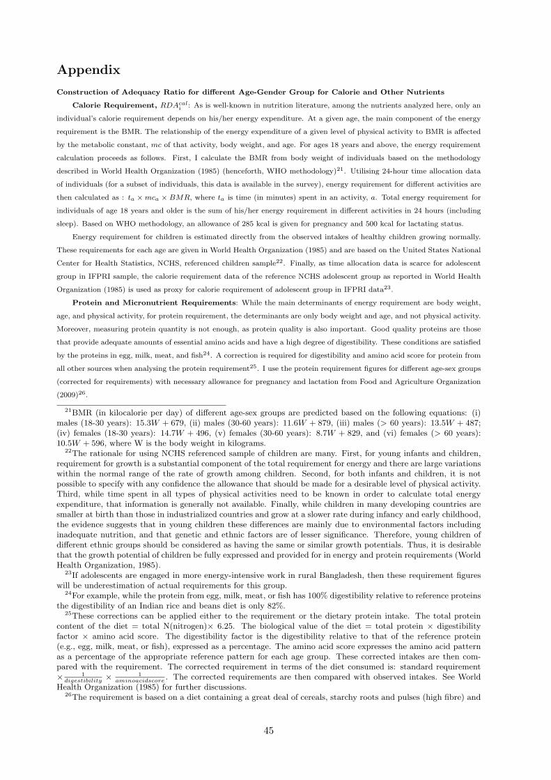
Appendix

Construction of Adequacy Ratio for different Age-Gender Group for Calorie and Other Nutrients

Calorie Requirement, RDAcali : As is well-known in nutrition literature, among the nutrients analyzed here, only an

individual’s calorie requirement depends on his/her energy expenditure. At a given age, the main component of the energy

requirement is the BMR. The relationship of the energy expenditure of a given level of physical activity to BMR is affected

by the metabolic constant, mc of that activity, body weight, and age. For ages 18 years and above, the energy requirement

calculation proceeds as follows. First, I calculate the BMR from body weight of individuals based on the methodology

described in World Health Organization (1985) (henceforth, WHO methodology)21. Utilising 24-hour time allocation data

of individuals (for a subset of individuals, this data is available in the survey), energy requirement for different activities are

then calculated as : ta × mca × BMR, where ta is time (in minutes) spent in an activity, a. Total energy requirement for

individuals of age 18 years and older is the sum of his/her energy requirement in different activities in 24 hours (including

sleep). Based on WHO methodology, an allowance of 285 kcal is given for pregnancy and 500 kcal for lactating status.

Energy requirement for children is estimated directly from the observed intakes of healthy children growing normally.

These requirements for each age are given in World Health Organization (1985) and are based on the United States National

Center for Health Statistics, NCHS, referenced children sample22. Finally, as time allocation data is scarce for adolescent

group in IFPRI sample, the calorie requirement data of the reference NCHS adolescent group as reported in World Health

Organization (1985) is used as proxy for calorie requirement of adolescent group in IFPRI data23.

Protein and Micronutrient Requirements: While the main determinants of energy requirement are body weight,

age, and physical activity, for protein requirement, the determinants are only body weight and age, and not physical activity.

Moreover, measuring protein quantity is not enough, as protein quality is also important. Good quality proteins are those

that provide adequate amounts of essential amino acids and have a high degree of digestibility. These conditions are satisfied

by the proteins in egg, milk, meat, and fish24. A correction is required for digestibility and amino acid score for protein from

all other sources when analysing the protein requirement25. I use the protein requirement figures for different age-sex groups

(corrected for requirements) with necessary allowance for pregnancy and lactation from Food and Agriculture Organization

(2009)26.

21BMR (in kilocalorie per day) of different age-sex groups are predicted based on the following equations: (i)males (18-30 years): 15.3W + 679, (ii) males (30-60 years): 11.6W + 879, (iii) males (> 60 years): 13.5W + 487;(iv) females (18-30 years): 14.7W + 496, (v) females (30-60 years): 8.7W + 829, and (vi) females (> 60 years):10.5W + 596, where W is the body weight in kilograms.

22The rationale for using NCHS referenced sample of children are many. First, for young infants and children,requirement for growth is a substantial component of the total requirement for energy and there are large variationswithin the normal range of the rate of growth among children. Second, for both infants and children, it is notpossible to specify with any confidence the allowance that should be made for a desirable level of physical activity.Third, while time spent in all types of physical activities need to be known in order to calculate total energyexpenditure, that information is generally not available. Finally, while children in many developing countries aresmaller at birth than those in industrialized countries and grow at a slower rate during infancy and early childhood,the evidence suggests that in young children these differences are mainly due to environmental factors includinginadequate nutrition, and that genetic and ethnic factors are of lesser significance. Therefore, young children ofdifferent ethnic groups should be considered as having the same or similar growth potentials. Thus, it is desirablethat the growth potential of children be fully expressed and provided for in energy and protein requirements (WorldHealth Organization, 1985).

23If adolescents are engaged in more energy-intensive work in rural Bangladesh, then these requirement figureswill be underestimation of actual requirements for this group.

24For example, while the protein from egg, milk, meat, or fish has 100% digestibility relative to reference proteinsthe digestibility of an Indian rice and beans diet is only 82%.

25These corrections can be applied either to the requirement or the dietary protein intake. The total proteincontent of the diet = total N(nitrogen)× 6.25. The biological value of the diet = total protein × digestibilityfactor × amino acid score. The digestibility factor is the digestibility relative to that of the reference protein(e.g., egg, milk, meat, or fish), expressed as a percentage. The amino acid score expresses the amino acid patternas a percentage of the appropriate reference pattern for each age group. These corrected intakes are then com-pared with the requirement. The corrected requirement in terms of the diet consumed is: standard requirement× 1

digestibility× 1

aminoacidscore. The corrected requirements are then compared with observed intakes. See World

Health Organization (1985) for further discussions.26The requirement is based on a diet containing a great deal of cereals, starchy roots and pulses (high fibre) and

45

Although required in small amounts, micronutrients are essential for life, and needed for a wide range of body functions

and processes. Age-sex specific RDA figures (with pregnancy and lactating allowance) for different micronutrients are

obtained from World Food Programme (2000). Analogous to quality of protein, sources of iron are important. Iron in meat

(haem iron) is more easily absorbed than iron contained in plant foods (non-haem iron). Trace minerals from the meat

sources have higher bio-availability and contribute to higher bio-availability of iron from plant sources. Similarly, nutrition

literature indicates that minerals and vitamins from meat sources are more highly bio-available than from plant sources.

Moreover, meat consumption can increase the bio-availability of minerals and vitamins contained in plant products when

meats and plants are consumed concurrently. I use the iron requirement figures that assumes very low iron bioavailability as

observed in South Asian Diet.

little complete (animal) protein as in the case of Bangladeshi diet.

46