UNDERSTANDING WATER QUALITY IN CITY WATER SYSTEMS USING ARCGIS

Jennifer SwitzerMGIS Capstone ProjectPenn State UniversityJuly 2016

BACKGROUND Chlorine (Cl2) is a common disinfectant used to kill microbes in drinking water due to its low

cost, stability and effectiveness (Al-Jasser 2007). When chlorine is added to a water system, a certain amount is used up between initial reactions with inorganic and organic material and metal in the water (Centers for Disease Control and Prevention 2014). The remaining chlorine, called free or residual chlorine, is available for disinfection of disease-causing organisms within the distribution network (Centers for Disease Control and Prevention 2014). The presence and amount of residual chlorine is a measure of the potability and quality of the water because it indicates that a sufficient amount of chlorine was initially added to inactivate diarrheal disease-causing bacteria and some viruses and that the water is protected from recontamination during storage (Centers for Disease Control and Prevention 2014) . Chlorine is a strong oxidizer and reacts with a wide variety of chemicals and naturally occurring organic/inorganic material which creates potentially harmful disinfection by-products (DBPs) (Goyal and Patel 2015). Since some of these DBPs are suspected carcinogens and cause reproductive and developmental problems, it is essential that a water authority manage its chlorine disinfection and use residual chlorine concentrations throughout the distribution system as a final check of water quality as it is delivered to customers (Goyal and Patel 2015).

As water moves through a water system, chlorine is expended as it interacts with microbes and pipe material which reduces the residual chlorine levels as it reaches the end of the distribution line (Turgeon, et al. 2004). The Environmental Protection Agency requires a "detectable" level of residual chlorine throughout a water system (EPA 2013). Measureable minimum levels vary by state, but all fall within the range of .05 mg/L to 0.5 mg/L (Aqua 2015). The Centers for Disease Control (2014) states that a level of 0.5 mg/L is enough residual chlorine to maintain water quality throughout the distribution network. Several sources, including Al-Jasser (2007), state that maintaining residual concentrations greater than 0.2 mg/L is necessary for sustained treatment throughout the pipe network. The EPA has set a maximum residual disinfectant level goal (MRDLG) such that chlorine must not exceed 4 mg/L in order to prevent health issues due to over disinfection.

Municipalities must have a detailed understanding of the water quality along their distribution system in order to recognize areas that may have chronically low residual chlorine levels and the possible reasons for this trend in order to implement changes to address any issues. Regular monitoring of residual levels helps operators understand the normal chlorine level patterns. Changes to patterns can indicate problems in the system, such as leakage of contaminants into the distribution network from main breaks or pipe leaks (Haas 1999).

OBJECTIVES The goal of this capstone project is to investigate the factors that affect residual chlorine

levels and model how these elements collectively contribute to water quality, all within Esri's

Page 2 of 34

ArcGIS environment. Water quality modeling is typically performed using expensive third party software and engineering consultants to build the model. Since GIS has become integral in managing and analyzing utility infrastructure, I want to determine if this project's workflow could be an alternative to using additional engineering modeling software and allow municipalities to better utilize their current investment in ArcGIS software to analyze water quality factors. I will examine pipe characteristics (material and diameter) and factors contributing to water age, including water turnover (volume of water contained in the pipe network versus water demand) and distance from the water source to determine where residual chlorine levels are the lowest. Lower chlorine levels are expected in areas farthest from the water source since this means the chlorine has a greater amount of time to interact with organic and inorganic materials and therefore be “used up” in the system (Turgeon, et al. 2004).

FACTORS RELATED TO CHLORINE RESIDUALS AND WATER QUALITY Water age is the primary factor in determining chlorine residuals and water quality. Water

age refers to the travel time of water after leaving the treatment plant and before entering the customers' plumbing system (Wang, et al. 2014). Chlorine can decay as water age increases, leaving low residual chlorine levels at distant parts of a distribution line (Masters, et al. 2015). Many variables contribute to water age, including water turnover and distance from the source (Wang, et al. 2014; Al-Jasser 2007). Pipe characteristics, such as material and diameter, can also affect water quality. (Wang, et al. 2014; Masters, et al. 2015; Al-Jasser 2007).

WATER TURNOVER/STAGNATION:An information paper by AWWA and Economic and Engineering Services (2002) discusses

the following design and water demand practices that contribute to water age. Many water systems are designed to not only meet current drinking water demands, but maintain pressures and quantities for firefighting and future needs. Cities commonly size pipelines and reservoirs to provide for water demand that will occur 20 years in the future. Maintaining proper water pressure and supply for fire flow and other emergencies requires installation of pipes with larger diameters even though smaller sizes would suffice for normal potable water delivery.

Water age can be effected by these planning measures because the increase in water volume exceeds the current demand that is cycled through normal consumer use. Changes in water demand or use patterns due to water conservation practices, relocation of a major water user or consolidation of multiple systems also greatly affect water turnover rates and water age. Even though fire flow requirements vary between cities, many communities opt to incur the cost of upsizing their system for fire protection to reduce possible property loss. The exact effects from fire flow planning vary by system, but these measures have a much greater impact on smaller distribution systems (AWWA; Economic and Engineering Services 2002).

Page 3 of 34

Disinfection by-products are more likely to form as water ages. This formation increases the water temperature, often causing higher chlorine demand since higher temperatures often increase reaction and growth rates (AWWA; Economic and Engineering Services 2002). Low water turnover, or stagnation, lengthens the time water remains in the distribution network which allows particles to settle and biofilm to grow (Mounce, et al. 2014; Shamsaei, Jaafar and Basri 2013). Oversized storage facilities, dead end pipes and areas with low water use promote stagnation (Mounce, et al. 2014).

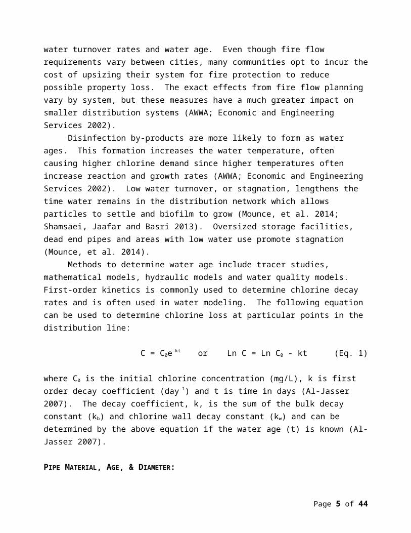
Methods to determine water age include tracer studies, mathematical models, hydraulic models and water quality models. First-order kinetics is commonly used to determine chlorine decay rates and is often used in water modeling. The following equation can be used to determine chlorine loss at particular points in the distribution line:

C = C0e-kt or Ln C = Ln C0 - kt (Eq. 1)

where C0 is the initial chlorine concentration (mg/L), k is first order decay coefficient (day-1) and t is time in days (Al-Jasser 2007). The decay coefficient, k, is the sum of the bulk decay constant (kb) and chlorine wall decay constant (kw) and can be determined by the above equation if the water age (t) is known (Al-Jasser 2007).

PIPE MATERIAL, AGE, & DIAMETER:Different pipe materials have different chemical reactions with disinfectants and,

therefore, have a big impact on pipe wall decay (Hallman, et al. 2002). Biofilms are layers of bacteria that attach themselves to pipe walls, trapping nutrients, microbes, worms, and water-borne pathogens that build upon themselves forming a plaque-like coating (Water Quality and Health Council n.d.). This build-up can clog water lines to the extent that adequate pressure is not able to be maintained for proper consumer or firefighting needs (Water Quality and Health Counciln.d.). The growth of biofilm on pipe walls is promoted differently depending on the pipe material due to varying degrees of roughness and chemical properties (Wang, et al. 2012).

The age of pipes in a distribution network greatly influences water quality and chlorine residuals due to corrosion of the pipe wall, which contributes to bacteria growth, leaching of metals into the water system and greater vulnerability to breakage (Water Quality and Health Council n.d.). Pipes installed in the early days of utility infrastructures were primarily made up of cement/cement lined (i.e. asbestos cement (AC), cement lined cast iron (CLCI)) or metallic (i.e. cast iron (CI), ductile iron (DI)) materials, which are more susceptible to corrosion.

Today, vinyl pipes are widely used due to their resistance to biofilm formation, resilience to harsh soil and weather conditions, and minimal failure rate (Water Quality and Health Council n.d.). A study by Al-Jasser (2007) studied pipe age effects on the wall decay constant and found that while service age impacted the wall decay on all types of pipe materials, effects were greatest in cast iron pipes, followed by steel, then cement, and then vinyl.

Page 4 of 34

Plastic pipes (i.e. polyvinyl chloride (PVC) and medium density polyethylene (MDPE)) and cement-based pipes are considered unreactive materials, whereas metals, like unlined cast iron, are classified as reactive, creating a reactive hierarchy where CI > DICL (Cement lined ductile iron) > PVC > MDPE (Hallman et al., 2002; Masters et al., 2015). The study by Wang et al. (2012) compared pipe material effects to opportunistic pathogen growth and the results were consistent with the general ranking that iron pipes have the most potential for bacterial re-growth, followed by cement and then PVC.

A pipe’s diameter and material “roughness” affect the flow of water through the distribution system. Based on general velocities used for pipe design, we can see the difference in the water velocity of pipes with 1-inch diameters being 3.5 ft/s versus a 12-inch diameter being 8.5 ft/s (The Engineering Toolbox n.d.). Friction loss is the loss in pressure, or head, inside of pipes due to flow, pipe diameter, length and roughness of internal pipe surface which is denoted by established roughness coefficients based on pipe material. EPANET modeling software uses head loss to analyze hydraulic components to model water quality (Rossman 2000). Turgeon et al. (2014) theorized that small diameter pipes encourage more interaction between water and pipe material, especially at points on the extremities of distribution lines, however the results of their study did not find a strong correlation between only the small pipe variable and water quality issues. DISTANCE:

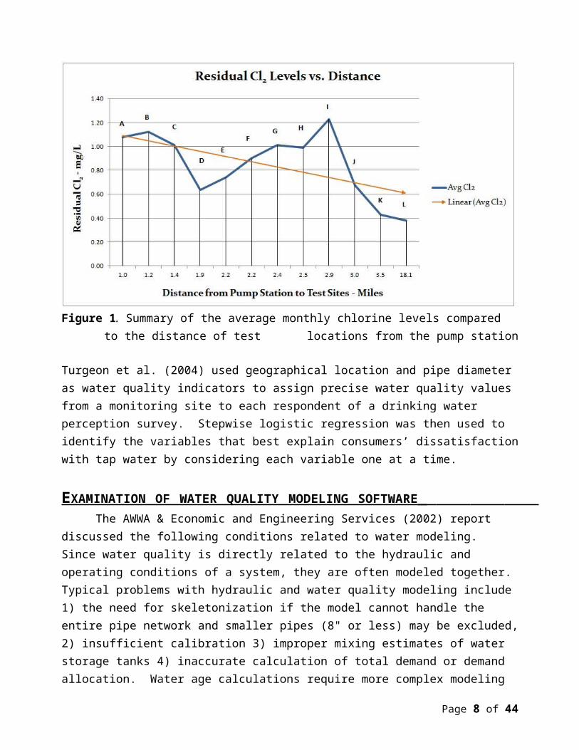
Residual chlorine concentrations decrease significantly the farther water travels through the system and can almost disappear in the farthest reaches of large distribution systems (Al-Jasser 2007; Turgeon, et al. 2004). Preliminary data analysis that I performed, using monthly chlorine test site samples over a 4 year period from 12 test locations, revealed that except for a few anomalies, there is an overall trend that chlorine levels degrade more the farther the test site is from the source (Figure 1). This observation supports the theory that longer pipe residence times allow chlorine to react with organisms and pipe materials that, in turn, promote chlorine decay.

Page 5 of 34

Figure 1. Summary of the average monthly chlorine levels compared to the distance of test locations from the pump station

Turgeon et al. (2004) used geographical location and pipe diameter as water quality indicators to assign precise water quality values from a monitoring site to each respondent of a drinking water perception survey. Stepwise logistic regression was then used to identify the variables that best explain consumers’ dissatisfaction with tap water by considering each variable one at a time.

EXAMINATION OF WATER QUALITY MODELING SOFTWARE The AWWA & Economic and Engineering Services (2002) report discussed the following

conditions related to water modeling. Since water quality is directly related to the hydraulic and operating conditions of a system, they are often modeled together. Typical problems with hydraulic and water quality modeling include 1) the need for skeletonization if the model cannot handle the entire pipe network and smaller pipes (8" or less) may be excluded, 2) insufficient calibration 3) improper mixing estimates of water storage tanks 4) inaccurate calculation of total demand or demand allocation. Water age calculations require more complex modeling and analysis of the water system and have high potential for inaccuracies.

Since the AWWA paper in 2002, water modeling has become more dynamic and complex, but also more commonly used by water utilities. A survey was conducted by the Engineering Modeling Applications Committee (EMAC) in 1999 to discover the current and planned uses for water distribution modeling and found that 80% of respondents planned to use GIS as a major source to develop hydraulic models versus only 15% that were currently using GIS (Ray, Jacobsen and Edwards 2014). A second survey, to see how water modeling had changed over the 14 year

Page 6 of 34

time period, was circulated in 2013 by the EMAC AWWA Water Distribution Model Survey Subcommittee of Ray, Jacobson and Edwards (2014). They found that 1) 63% of respondents create their hydraulic model from GIS and 56% update the model from GIS; 2) models are more detailed due to the use of GIS, increased processing speeds and data storage, explaining the change from 66% use of skeletonized models in 1999 versus only 19% in 2013; 3) 70% of respondents in 2013 use extended-period simulation (EPS) analysis versus 50% in 1999 which requires demand usage patterns and operational controls. Even though modeling has improved over the years, challenges still remain. In the 2013 survey, 42% of respondents said calibration, which involves adjusting the model after comparing field measurements to model results, was the most technically challenging aspect of hydraulic modeling. Even though utilities are the primary users of hydraulic models, 54% of those surveyed said a consulting firm was used to create their model.

Numerous software applications are available for hydraulic water quality modeling. EPANET is a free, public domain software package that runs on Windows 95/98/NT/XP and performs extended period simulation of water movement and quality in distribution systems with visualization of simulation results (EPANET 2015). Numerous studies have used EPANET to predict chlorine concentrations; however the software is not formally supported, runs on outdated operating systems and requires manual digitization of the pipe network inside the software or importing a text file of a basic network instead of easily importing data from GIS (Rossman 2000). Monteiro et al. (2014) used the EPANET Multi-Species Extension (EPANET MSX) to model chlorine residuals using a more complex mathematical decay model. EPANET MSX is an extension to EPANET which allows the user to manually define the chemical reactions for wall decay and reaction equations that are most relevant to his/her study (Monteiro, et al. 2014). Monteiro found that EPANET MSX greatly improved modeling capabilities; however it was not user-friendly due to the lack of a graphical user interface for visualization of chlorine concentrations along the water network. A 3D-enabled EPANET Java web app was needed to work around this problem.

InfoWater by Innovyze, an Esri partner, is a distribution modeling and management software application that executes within the ArcGIS environment. The software allows for fire flow and water quality simulations, energy cost analysis, pressure zone management, and many other advanced analysis techniques (Innovyze 2015). The Multi-Species Extension (MSX) is similar to EPANET MSX which allows for modeling chlorine concentrations and other chemical reactions (Innovyze 2015).

WaterCAD by Bentley is hydraulic modeling software based in the CAD environment and is a subset of WaterGEMS, which runs the model within ArcGIS (Bentley n.d.). These applications create water quality simulations and help evaluate current and proposed water system design and operations. A study by Hamdy, Moustafa and Elbakri (2014) used WaterCAD to analyze a water network in Egypt and was able to effectively determine the lowest needed chlorine dosing amount to maintain sufficient chlorine residuals while reducing disinfection costs. The first order kinetic model used by WaterCAD to determine chlorine decay due to pipe interactions is the same as the

Page 7 of 34

broadly-used equation outlined in the previous section on water age, C(t) = C0e-kt , where C(t) is the chlorine concentration at time t (mg/L), C0 is the initial concentration and t is the resistance time in the pipe (Hamdy, Moustafa and Elbakri 2014).

The software applications outlined above offer extensive lists of modeling and reporting capabilities, however the components may be excessive for smaller municipalities that need an understanding of water quality within their distribution system, but may not have the money or personnel to purchase and effectively utilize the software. The small municipality for which I work considered hiring an engineering consultant to create a hydraulic/water quality model based in WaterCAD. In order for us to maintain this model, we inquired about purchasing the software and received a quote from Bentley in September 2015 for WaterCAD. The initial purchase price for the smallest network size (2000 pipes) would have been about $8,500 with an ongoing yearly subscription fee of around $2,100. These numbers only include the software and do not consider the time and training of city personnel to run and maintain the model or the price of hiring the engineering consultant to set up the model, which would have been a six figure cost. In addition, CAD-based products can import GIS-based data, but the conversion from an ArcGIS geodatabase feature class to a CAD drawing file format adds nine additional fields to the attribute table to describe drawing styles and, in my conversion testing, drops several of the original GIS fields. Since GIS has become integral in managing, analyzing and planning utility infrastructure assets, a municipality should be able to fully utilize their current investment in standard GIS software to gain an understanding of the infrastructure affects on the quality of water delivered to customers.

DATA SOURCES Municipal water systems are fed by a water source, such as a lake, then disinfected at a

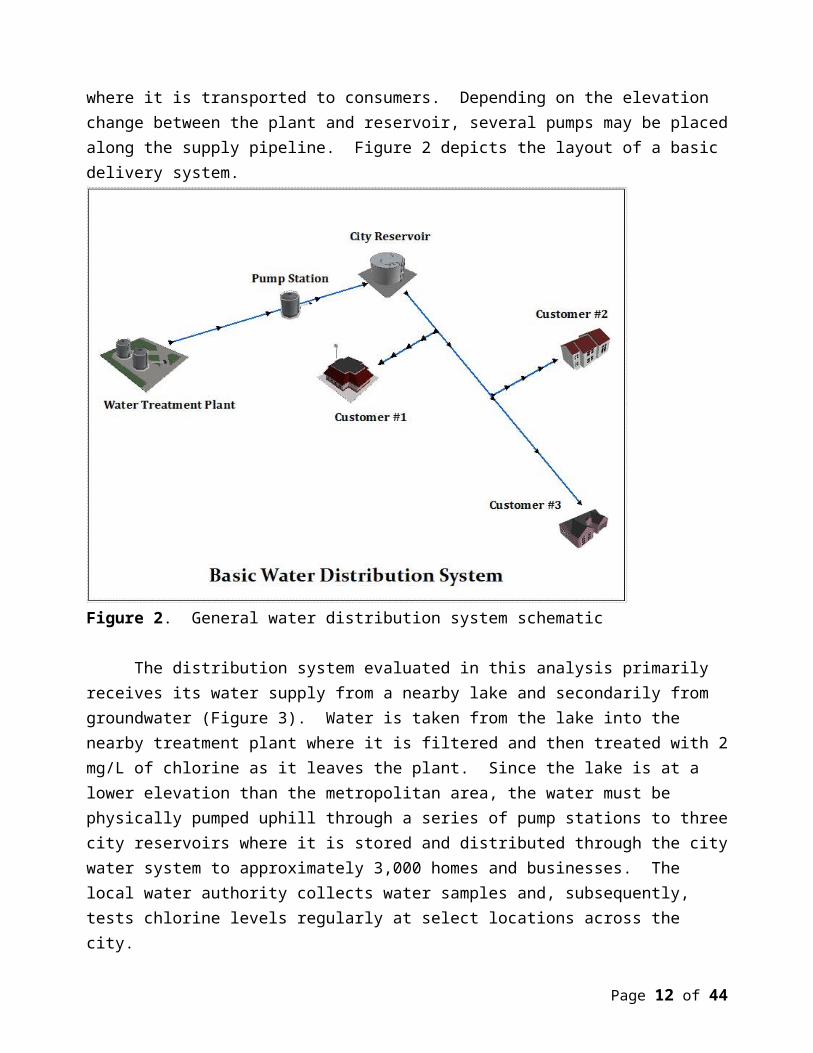
water treatment plant and pumped to a city storage facility before entering the delivery network. Reservoirs are elevated above the distribution system where gravity pulls the water from the storage tank and into the water network where it is transported to consumers. Depending on the elevation change between the plant and reservoir, several pumps may be placed along the supply pipeline. Figure 2 depicts the layout of a basic delivery system.

Page 8 of 34

Figure 2. General water distribution system schematic

The distribution system evaluated in this analysis primarily receives its water supply from a nearby lake and secondarily from groundwater (Figure 3). Water is taken from the lake into the nearby treatment plant where it is filtered and then treated with 2 mg/L of chlorine as it leaves the plant. Since the lake is at a lower elevation than the metropolitan area, the water must be physically pumped uphill through a series of pump stations to three city reservoirs where it is stored and distributed through the city water system to approximately 3,000 homes and businesses. The local water authority collects water samples and, subsequently, tests chlorine levels regularly at select locations across the city.

Page 9 of 34

Figure 3. Overview of water sampling test site locations and primary water line feeds

Page 10 of 34

Data used for this study includes chlorine results from water samples taken at 12 testing sites and the last pumping station from the treatment plant, the GIS water system infrastructure data to obtain the location, length, diameter, and material of pipes in the delivery system, unofficial daily chlorine tests from reservoirs, daily totals of the amount of water pumped to the reservoirs from the treatment plant that is needed to replenish supply and maintain minimum water levels in the tanks, and metered water usage at each site from the city's utility department.

TEST SITE DATA:Official residual chlorine test results were acquired for four locations (C, J, K, & L) that were

collected once a month on a quarterly basis between April 2012 and April 2015 and 10 sites (A, B, C, D, E, F, G, H, I, L) that were sampled twice a month, 7-8 months out of the year between June 2012 and Oct 2015 (Figure 3). Sites C and L were tested during both rounds of sampling. In October 2014, site J was taken out of testing, so data for this site does not extend to 2015.

The test results arrived in Excel worksheets and PDF documents for each test location with a list of the individual test dates and the corresponding chlorine values. All the data was consolidated into Microsoft Excel where I calculated chlorine averages and standard deviations in order to graph the results against influencing factors. I created a point feature class in an Esri file geodatabase of all the sites for the months that compose a season in order to include data from all test sites over similar temperature and water usage patterns (i.e. June, July, August span the summer months and will encompass test results from all sites).

PUMP STATION AND RESERVOIR DATA:The pump station included in this analysis is the last in a series of pumps that help deliver

the water from the treatment plant to the city reservoirs. Chlorine levels at the pump station were provided as monthly averages by the treatment plant supervisor. I used the pump station’s chlorine levels for the same months that samples were taken at the test locations. The city collects daily water samples from each reservoir and tests the chlorine levels as the water exits the tanks. However, these tests are unofficial and the residual chlorine values tend to be lower than chlorine levels at the test sites, indicating either error in data collection or poor circulation within the tank. Since I was not confident in the reservoir chlorine readings, I used them for reference, but did not feel they could be relied upon to determine decay values.

Therefore, I used the pump station as the intermediate water source between the treatment plant and the distribution system to determine the water system’s beginning chlorine level for the analysis. The pump's chlorine levels will be used to measure the changes in chlorine values from an initial source to the point of extraction from the water system. We can assume that chlorine levels are diminished as the water sits in the reservoirs before it is distributed.

Page 11 of 34

WATER LINE DATA:I exported the pipes that ran from the pump station, to the related reservoirs, to each test

site in order to capture the distance the water travels from the intermediate source to the final destinations and stored them in a line feature class for the all the test sites. A separate feature class was created to contain the main line from the treatment plant to the pump station so that I could determine the amount of chlorine decay from the initial source to the intermediate source before it enters the city’s water distribution system. Using this information, I calculated the total length of pipe involved for each test site so that I could compare the chlorine values to the distance traveled by the water.

DATA ANALYSIS METHODS The objective of this analysis is to compare the relationship of chlorine concentrations from

the pump station and reservoirs to locations throughout the city to quantify where and why residual chlorine levels in the system vary and to determine if this study could be used as a low cost alternative to using additional modeling software to analyze and model factors that affect residual chlorine levels. Analyzing the data across all the months throughout the year may skew the analysis, since temperatures and watering behaviors change with each season and, thus, may affect the amount of water being consumed and the residual chlorine levels. I calculated the average monthly residual chlorine values and standard deviation across all years (i.e. average of July 2012, July 2013, and July 2014) and plotted these averages against the test months for each site in order to identify any data trends at each location and overall trends across the city. In order to normalize the data for a more accurate comparison between test sites and to incorporate readings from all the sites over a similar time period, I compared the average seasonal residual chlorine levels for the summer months of June, July and August. I looked at the factors of water travel distance within the pipelines, pipe material, diameter, and the turnover rate in the pipe networks for each reservoir to analyze the chlorine level variations. When comparing factors like material and diameter, sites located within similar distances from the pump station were compared together in order to negate the effect of distance on the chlorine values.

Page 12 of 34

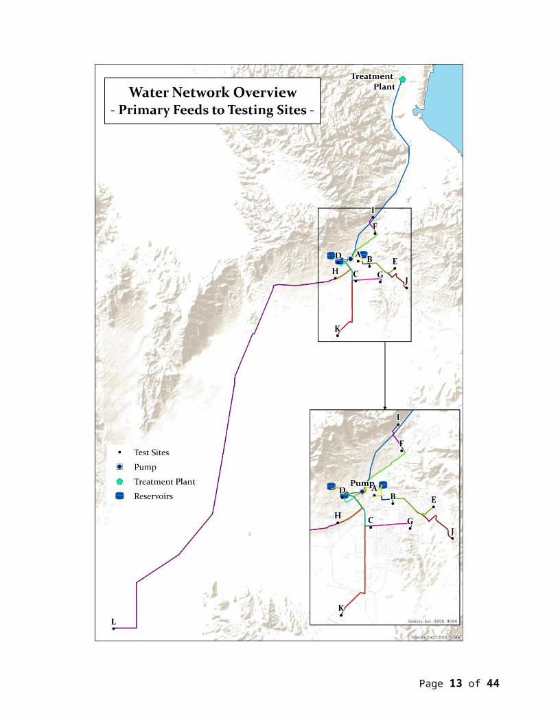
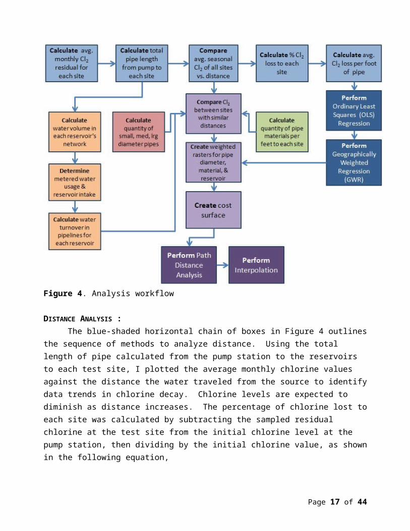
Figure 4. Analysis workflow

DISTANCE ANALYSIS :The blue-shaded horizontal chain of boxes in Figure 4 outlines the sequence of methods to

analyze distance. Using the total length of pipe calculated from the pump station to the reservoirs to each test site, I plotted the average monthly chlorine values against the distance the water traveled from the source to identify data trends in chlorine decay. Chlorine levels are expected to diminish as distance increases. The percentage of chlorine lost to each site was calculated by subtracting the sampled residual chlorine at the test site from the initial chlorine level at the pump station, then dividing by the initial chlorine value, as shown in the following equation,

Percent Cl2 loss = (Initial Cl2 - Final Cl2)/Initial Cl2 (Eq. 2)

In order to incorporate chlorine values with the pipe features, I added a field for chlorine loss per foot to the water line attribute table and used the field calculator to populate the records by multiplying the shape_length field by the amount of Cl2 loss. This assigned a value for chlorine loss to each pipe feature along each site's main distribution line.

Page 13 of 34

PIPE ANALYSIS:To evaluate the effects of pipe material on residual chlorine, as shown in the green box in

Figure 4, I calculated the amount of each pipe material per feet along the primary lines to each site. Then, using the following equation, I determined the percentage of each material compared to the total amount of pipe,

% pipe material = (Total feet of material/Total feet of entire pipeline)*100 (Eq. 3)

Similarly, I calculated the amount of pipe (in feet) with different sized diameters and determined the percentage of pipe per diameter category of the total pipeline to each test site. I used graphical trend analysis to compare the material and diameter amounts between sites of similar distances in order to identify possible correlations to help assign an influence weight to these factors.

WATER USAGE:To study the effects of water usage, I followed the orange-shaded chain of boxes in Figure

4 and calculated the volume of water contained in the pipe network between the city reservoirs and testing locations. I categorized the pipes by diameter size and then applied the following volume formula

.785 (d2) (l) = ft3 (Eq. 4)

where d = diameter and l = length. The volume of each pipe category was summed to determine the total water volume to each test site and then the entire network for each reservoir. Using the monthly metered water usage collected by the city's utility department, I looked at how the chlorine residuals varied between sites of similar distance from the pump station. To approximate the water turnover in the pipes for each reservoir, I compared the volume in the pipe network to the amount of water pumped into the reservoir to replace used water. The percent water turnover within the reservoir networks was calculated by the following formula

Network Turnover = (RW/PV) * 100 (Eq. 5)

where RW = Avg monthly water pumped into reservoir and PV = Total volume in pipes for reservoir. Since two of the three city reservoirs serve the same areas of town, I considered them one reservoir for the turnover analysis.

REGRESSION ANALYSIS:Regression analysis was performed after distance analysis calculations and is depicted in

the dark blue boxes in Figure 4. With the dependent variable, chlorine loss per foot, joined to the same feature dataset as the explanatory factors of distance (length), diameter, material, and

Page 14 of 34

source (turnover), Ordinary Least Squares (OLS) regression was used to create a global model that examined the relationship and influence of these factors. OLS is commonly the first step in spatial regression analysis in which a single regression equation is created to model a process across the entire study region and predict the dependent variable (Esri 2013). Logistic regression is best used to determine the presence or absence of an event based on several variables, either continuous (measurable elements such as distance or time) or categorical (such as pipe material or diameter) (Turgeon, et al. 2004).

Initially, I used the waterlines as they existed to run Ordinary Least Squares regression; however it did not result in a significant model. In order to get a more significant model, I standardized the pipelines by creating more even waterline segments to use in the regression analysis. The original waterlines varied greatly in length in which some segments were very long and others were short. Since chlorine loss per foot was calculated using the length of the pipe segments, the length variations caused a more significant influence on the chlorine loss than any other factor. Therefore, the affect of pipe length needed to be neutralized in order to consider the affects of additional factors on the chlorine loss. First, I removed extra vertices using the "Generalize" tool in the Editing toolbox. A 4 ft tolerance was used to minimize the vertices without greatly affecting the spatial accuracy of the pipeline features. Vertices were then added approximately every 100 feet using the "Densify" tool with a 100 max distance. Finally, the lines were split at the vertices using the "Split Line at Vertices" tool under the Data Management → Features toolbox. The amount of Cl2 lost per each 100 foot segment of pipe was determined using the field calculator by multiplying the length of each feature by the rate of Cl2 lost per foot. Since each test site had a different rate of Cl2 loss, I averaged the loss rate on common main lines based on the rate of loss for each site along that line.

In order to run the OLS tool, the attribute table must contain a unique ID field other than the ObjectID and the explanatory variables must be in numerical form. I added integer fields to describe the pipe material and source (reservoir turnover). Using the relationships observed in the graphical trend analysis, I assigned low values to less effective factors and higher values to more effective factors. The values for pipe material were assigned based on pipe reactivity such that PVC (least reactive) = 1, Cement = 2, Steel = 3, Iron (most reactive) = 4. The source values were assigned based on the theory that more water turnover means higher chlorine values; therefore pipelines fed by Reservoir #2 = 5 and Reservoir #1 = 6. I originally assigned values of 1 and 2 respectively, but the Geographically Weighted Regression tool failed to run because the values were identical to integers assigned to pipe material.

The OLS tool ran with chlorine loss per foot, determined using the summer month calculations, as the dependent variable and material, diameter, source, and length as explanatory variables. I ran many iterations with different combinations of these variables to find a model that worked well. To ensure I found the optimal combination, I used the Exploratory Regression tool which checked all possible combinations of the variables and found the relationships and

Page 15 of 34

significance of each. Finally, the Moran's I tool was run on the residuals to see if they were normally distributed using the following parameters:

Input field = Residuals Conceptualization = Inverse Distance Distance Method = Manhattan Standardization = Row Distance Band = 300

Since all the model iterations did not have normally distributed residuals, I ran the Incremental Spatial Autocorrelation tool. It determined that a band distance of 300 was best to use because this is where the first Z-score peak occurred in the graph. The peaks on the graph represent the distances at which the spatial processes that encourage clustering are the most prominent (Esri n.d.).

To create a local regression equation for each feature in the dataset, I used Geographically Weighted Regression (GWR) which provides statistics on the linear relationships between variables (Esri 2013). GWR does not work with line features. Therefore, I used the "Feature to Point" tool in the Data Management → Features toolbox to convert the pipelines to points. I ran GWR using the following parameters:

Dependent variable = Cl2 loss per foot Explanatory variables = diameter and material (GWR failed to execute when the

Source variable was included) Kernel = Fixed Bandwidth = AICc

These regression techniques help determine the amount of negative or positive influence certain factors have on the dependent variable and help predict values at un-sampled locations (Esri 2013). The relationships revealed with these processes were used to determine weights to create a cost surface for path distance analysis.

PATH DISTANCE ANALYSIS & INTERPOLATION:Path distance analysis determines the accumulative "cost" of travel from a source to each

cell on a raster by considering a cost surface (weighted cell values for certain factors) and the surface distance (elevation layer) (Esri 2011). The chain of light and dark purple boxes in Figure 4 outline the process for path distance analysis and interpolation. Raster layers were created from the water line feature class in which weights were assigned to certain features based on their degree of influence as determined by the relationships discovered from graphical trends and regression analyses of pipe material, diameter, distance, and turnover. Factors with little influence were given a low weight and factors with greater influence were given higher weights. The “Raster Calculator” tool was used to combine the weighted rasters to create an overall cost surface layer. The "Path Distance Analysis" tool in the Spatial Analyst → Distance toolbox was run

Page 16 of 34

with the test site locations as the input features, a DEM as the input surface raster, and the Cost Surface as the input cost raster.

Interpolation creates a continuous surface of predicted values based on a sample set of data points using the degree of dependence of near and distant objects/values (Childs 2004). Since chlorine values are spatially related to values at nearby test sites, I used the kriging interpolation method in the ArcGIS Spatial Analyst toolbox to model the overall dispersion of chlorine across the entire water network with the following parameters:

Input point features = Test sites Z value field = Cl2 loss per foot Kriging Method = Ordinary Semivariogram model = exponential Cell size = 100 Variable radius with 12 points

The exponential semivariogram model is meant to be used when autocorrelation decreases exponentially with distance (Esri - Kriging n.d.).

RESULTS SEASON AND DISTANCE ANALYSIS:

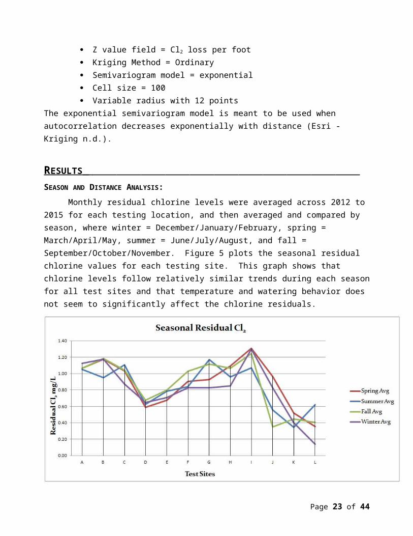
Monthly residual chlorine levels were averaged across 2012 to 2015 for each testing location, and then averaged and compared by season, where winter = December/January/February, spring = March/April/May, summer = June/July/August, and fall = September/October/November. Figure 5 plots the seasonal residual chlorine values for each testing site. This graph shows that chlorine levels follow relatively similar trends during each season for all test sites and that temperature and watering behavior does not seem to significantly affect the chlorine residuals.

Page 17 of 34

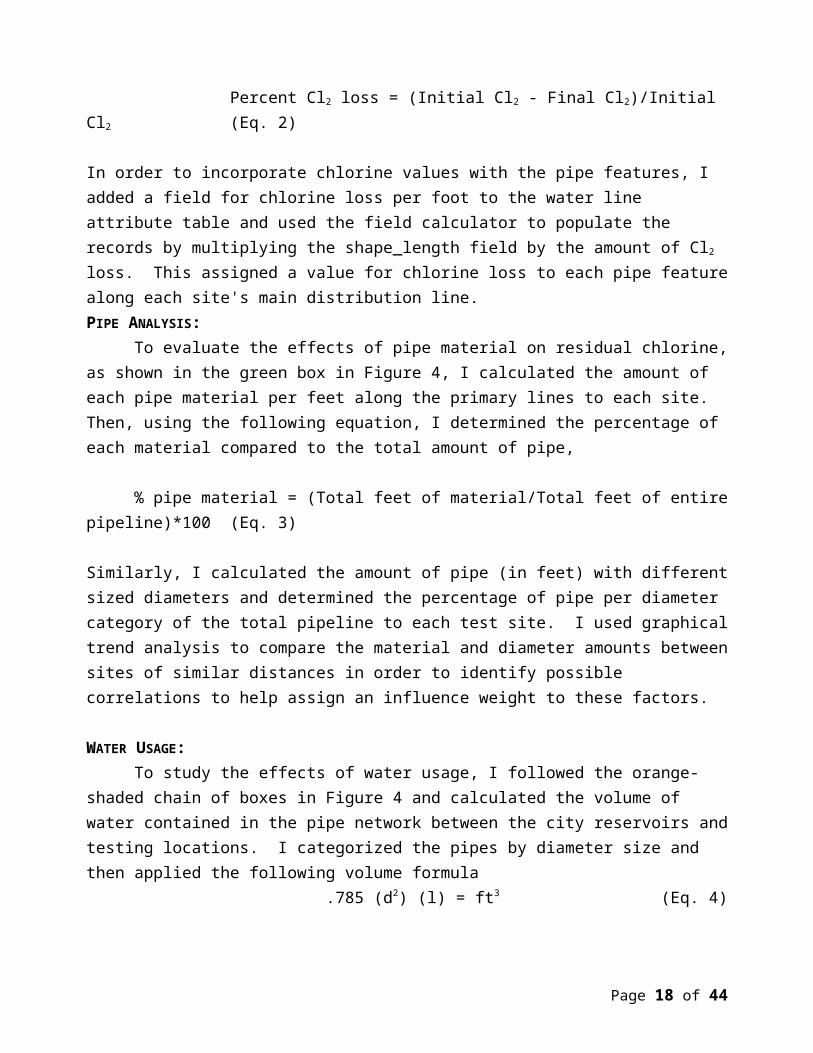
Figure 5. Seasonal residual chlorine averages for all test sites

The map in Figure 6 displays the spatial layout of testing sites and the corresponding percent of chlorine that is lost between the pump station and test locations. Looking at sites within similar distances to the pump station, we observe several inconsistencies. For example, site D experiences significantly more chlorine loss (54%) than comparable sites such as A, B, and C (19% -27% loss), indicating that additional factors are contributing to the chlorine decay at site D. Similarly, sites I and J only have a distance difference of 0.1 miles, but site I only experiences 11% chlorine loss while site J has 51% loss. Another anomaly is present between sites K and L. Water has 14.6 more miles to travel to reach site L, however there is only a 3% difference in residual chlorine loss between the sites. Further analysis on pipe characteristics and water usage will seek to explain why sites like D, I, and L defy the trend of decreasing residual values with increasing distance.

Page 18 of 34

Figure 6. All testing sites with percent residual chlorine loss

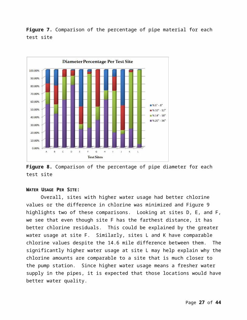
PIPE ANALYSIS:Comparing the change in chlorine values with the percentage of pipe material and

diameter sizes did not reveal significant correlations between the two factors. Figure 7 reveals

Page 19 of 34

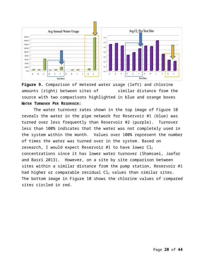
that nine out of ten sites had over 97% asbestos cement pipe (ACP), while only one site (site L) had 87.7% polyvinyl chloride (PVC). This does not look like a significant factor unless you compare sites K and L. They have similar residual chlorine loss despite the fact that water has to travel over 14 more miles to reach site L. The pipeline to site L is primarily composed of plastic compared to the old cement lines to site K. This may be contributing to the more even chlorine loss. The diameter analysis in Figure 8 did not expose a clear trend between the test sites' chlorine values and the percentage of different pipe diameters, therefore diameter does not seems to be a significant factor in chlorine residual variations.

Figure 7. Comparison of the percentage of pipe material for each test site

Page 20 of 34

Figure 8. Comparison of the percentage of pipe diameter for each test site

WATER USAGE PER SITE: Overall, sites with higher water usage had better chlorine values or the difference in

chlorine was minimized and Figure 9 highlights two of these comparisons. Looking at sites D, E, and F, we see that even though site F has the farthest distance, it has better chlorine residuals. This could be explained by the greater water usage at site F. Similarly, sites L and K have comparable chlorine values despite the 14.6 mile difference between them. The significantly higher water usage at site L may help explain why the chlorine amounts are comparable to a site that is much closer to the pump station. Since higher water usage means a fresher water supply in the pipes, it is expected that those locations would have better water quality.

Figure 9. Comparison of metered water usage (left) and chlorine amounts (right) between sites of similar distance from the source with two comparisons highlighted in blue and orange boxes

Page 21 of 34

WATER TURNOVER PER RESERVOIR:The water turnover rates shown in the top image of Figure 10 reveals the water in the pipe

network for Reservoir #1 (blue) was turned over less frequently than Reservoir #2 (purple). Turnover less than 100% indicates that the water was not completely used in the system within the month. Values over 100% represent the number of times the water was turned over in the system. Based on research, I would expect Reservoir #1 to have lower Cl2 concentrations since it has lower water turnover (Shamsaei, Jaafar and Basri 2013). However, on a site by site comparison between sites within a similar distance from the pump station, Reservoir #1 had higher or comparable residual Cl2 values than similar sites. The bottom image in Figure 10 shows the chlorine values of compared sites circled in red.

Figure 10. Comparison of water turnover per reservoir (top) and the average chlorine values per site with compared sites circled in red (bottom).

Page 22 of 34

REGRESSION ANALYSIS:Many model iterations were tested with Ordinary Least Square regression, however almost

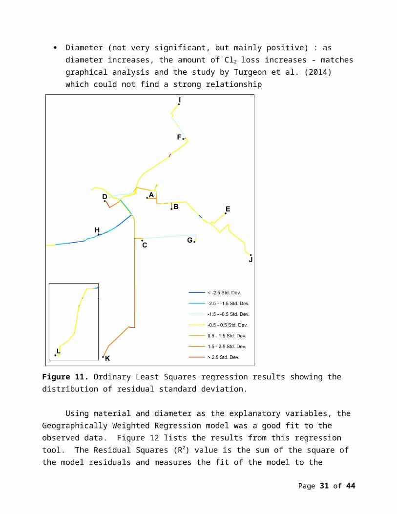
all the models did not have normally distributed residuals (difference between an observed value and the estimated value), meaning the models were biased. One model using the un-split water lines had normally distributed residuals, but the model was not significant. After running OLS with different combinations of explanatory variables, I ran the "Exploratory Regression Analysis" tool using all the possible explanatory variables on both the split water lines and the original lines to make sure I was finding the right fit. I then re-ran OLS using the combinations that ranked highest on the exploratory regression report. The best model used the water pipes that were split at approximately 100 ft increments with the explanatory variables of material, diameter, source, and length fields. All variables were statistically significant with the AICc = -19148.18 and Adjusted R-Squared value = .73. The Akaike Information Criterion (AICc) is a widely used mathematical statistic to measure model performance. The lower the AICc value the better the model. The Adjusted R-Squared value also describes model performance and ranges from 0.0 to 1.1 (Esri 2014). A value of .73 means that the model (explanatory variables) explains 73% of the variation in the dependent variable (Cl2 loss) (Esri 2014). The residuals displayed positive spatial autocorrelation, meaning similar predictions were clustered together, which made the model biased. However, this is hard to avoid with linear features in which pipes of the same length, diameter, and material are going to be near each other, thus resulting in similar predictions being clustered together. Figure 11 displays the residual standard deviation pattern found in the OLS result.

The overall results revealed that the material, length and source variables were the most significant across all the models and diameter was only somewhat significant. The relationships found from the OLS process coincided with my results from the data trend analysis:

Material (+) : the more reactive the pipe material, the more Cl2 is lost - matches research and graphical analysis

Length (mostly +) : as length increases, more Cl2 is lost - matches research and graphical analysis

Source/Turnover (-) : the reservoir with greater turnover had more Cl2 loss - contradicts theory, but matches graphical analysis

Diameter (not very significant, but mainly positive) : as diameter increases, the amount of Cl2 loss increases - matches graphical analysis and the study by Turgeon et al. (2014) which could not find a strong relationship

Page 23 of 34

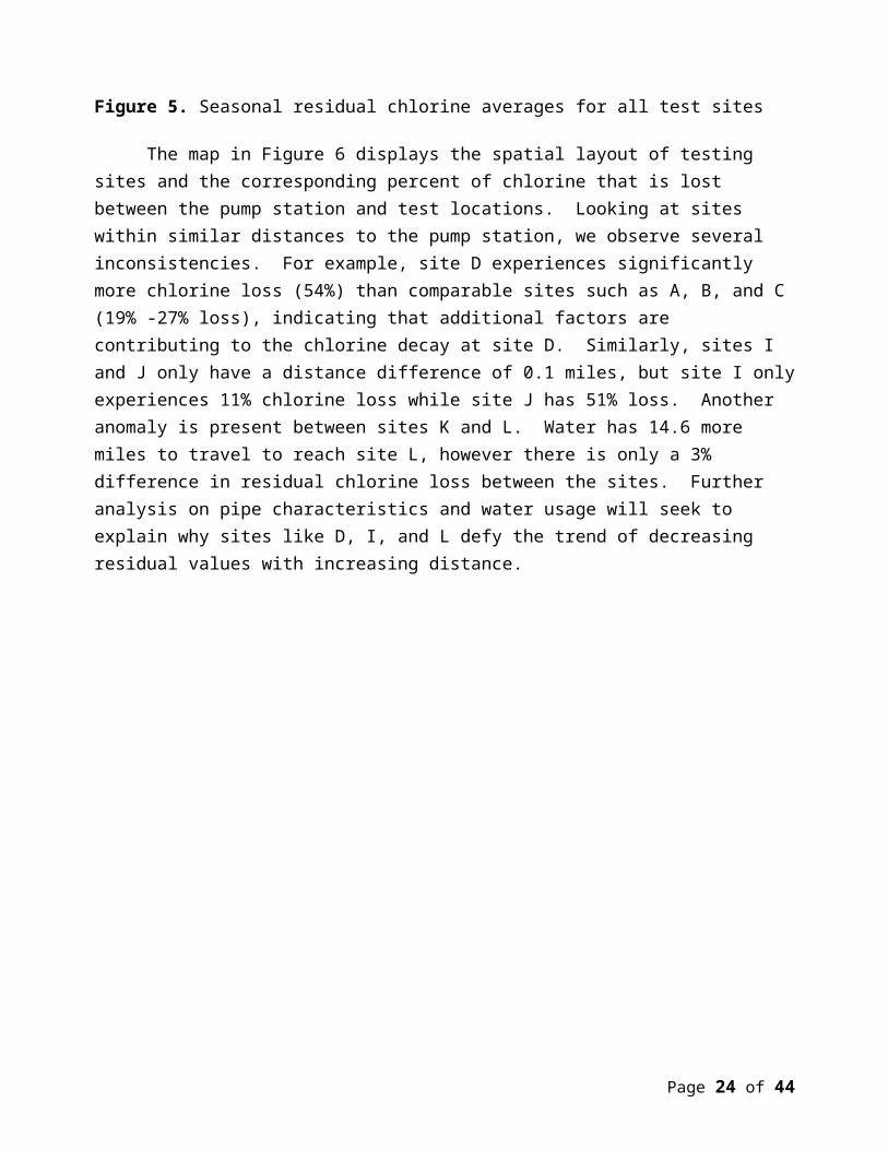
Figure 11. Ordinary Least Squares regression results showing the distribution of residual standard deviation.

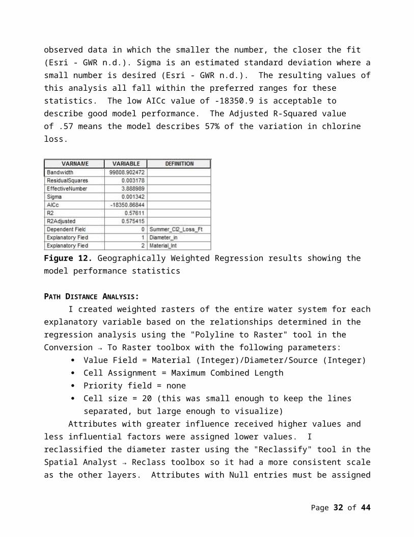
Using material and diameter as the explanatory variables, the Geographically Weighted Regression model was a good fit to the observed data. Figure 12 lists the results from this regression tool. The Residual Squares (R2) value is the sum of the square of the model residuals and measures the fit of the model to the observed data in which the smaller the number, the closer the fit (Esri - GWR n.d.). Sigma is an estimated standard deviation where a small number is desired (Esri - GWR n.d.). The resulting values of this analysis all fall within the preferred ranges for these statistics. The low AICc value of -18350.9 is acceptable to describe good model performance. The Adjusted R-Squared value of .57 means the model describes 57% of the variation in chlorine loss.

Page 24 of 34

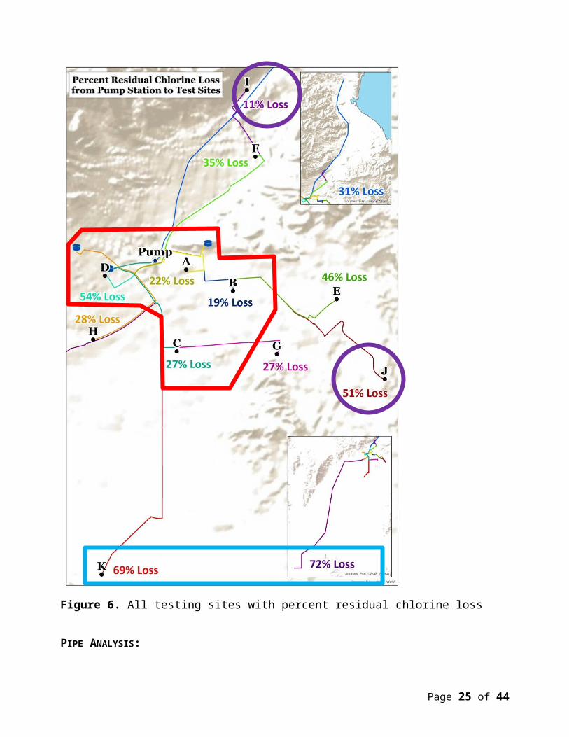
Figure 12. Geographically Weighted Regression results showing the model performance statistics

PATH DISTANCE ANALYSIS:I created weighted rasters of the entire water system for each explanatory variable based

on the relationships determined in the regression analysis using the "Polyline to Raster" tool in the Conversion → To Raster toolbox with the following parameters:

Value Field = Material (Integer)/Diameter/Source (Integer) Cell Assignment = Maximum Combined Length Priority field = none Cell size = 20 (this was small enough to keep the lines separated, but large enough to

visualize)Attributes with greater influence received higher values and less influential factors were

assigned lower values. I reclassified the diameter raster using the "Reclassify" tool in the Spatial Analyst → Reclass toolbox so it had a more consistent scale as the other layers. Attributes with Null entries must be assigned a value in order for that feature to be included in the Path Distance analysis.

Material: PVC = 1, Cement = 2, Steel = 3, Iron = 4 Diameter: grouped diameter sizes such that

1"-4" = 1 (these are technically laterals, but can still be included in the analysis)6" & 8" = 210" & 12" = 314", 16", 18" = 420", 24" = 5

Source (turnover): Reservoir #1 = 1, Reservoir #2 = 2 - this is the opposite weight to what I had originally assigned for OLS. I switched the values based on the OLS observation that the source variable had a negative relationship.

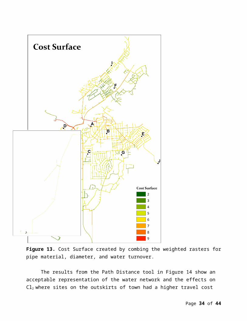
The Cost Surface in Figure 13 was created using the raster calculator to add each of the weighted rasters. I had first tried multiplying the diameter raster by .25 (25%) because it had less influence on Cl2 than the other factors and the material raster by .75 (75%) before adding all the rasters together. After running the path distance tool with this as the cost surface, it gave me an

Page 25 of 34

empty raster. So for the final product, I did not multiply any rasters by percentages and simply added them together.

Figure 13. Cost Surface created by combing the weighted rasters for pipe material, diameter, and water turnover.

The results from the Path Distance tool in Figure 14 show an acceptable representation of the water network and the effects on Cl2 where sites on the outskirts of town had a higher travel cost than locations in the central part of the city. However, it did not show variations on the paths

Page 26 of 34

to the test sites that were out of pattern to what would be expected based on the distance to the source (Al-Jasser 2007; Turgeon, et al. 2004). For example, test site D has low Cl2 values despite the fact that it is close to the reservoir (less distance to travel assumes higher Cl2 values). However, the path distance analysis did not show the area around D as being a potential problem area. I think two major factors that affected this were the low water usage and the dead-end location. I tried testing this theory by using the reservoir turnover relationship because it could be applied to all areas of the water system. I also experimented with adding a dead-end variable which pointed out areas that did not have any other water users except for the test location since this has a big effect on water turnover. However, when I ran OLS with this dead-end variable, it was not significant.

Figure 14. Results of Path Distance Analysis showing the "cost" of travel from the source locations

Page 27 of 34

INTERPOLATION:I first tried creating an interpolated surface using the Interpolation with Barriers tool,

however the output was incomplete or it gave an error. I experimented with using a cost surface that only included the main lines to the test sites, but this resulted in an error saying "weight parameter is too small". I also tried the cost surface created from the entire water system, but the output was incomplete.

Since diffusion interpolation produced incomplete results, I instead used the Kriging technique with an exponential semivariogram. I experimented with this model and the spherical semivariogram model which assumes autocorrelation decreases with distance until a certain point (Esri - Kriging n.d.). The surfaces produced from the spherical semivariogram did not predict data values that I would expect to see in a distribution model. For example, the spherical interpolated value range limits were much lower than the control point values, whereas the surfaces generated with the exponential semivariogram produced value limits that correlated more with the original chlorine levels. Interpolated surfaces were created for spring, summer, fall and winter chlorine values, as shown in Figure 15. The monthly surfaces were then combined for each year using the Cell Statistics tool to determine the predicted yearly mean values and an overview of the system shown in Figure 16. This surface displays the expected residual chlorine values across the city based on the measured levels at the test sites. It provides a way to visualize the areas of town that are prone to lower chlorine values (yellow/orange/red) which could imply poorer water quality. Utility managers may use this to identify areas that need chlorine testing, maintenance activities to flush stagnant water from the lines, or capital improvement projects to update the infrastructure.

Page 28 of 34

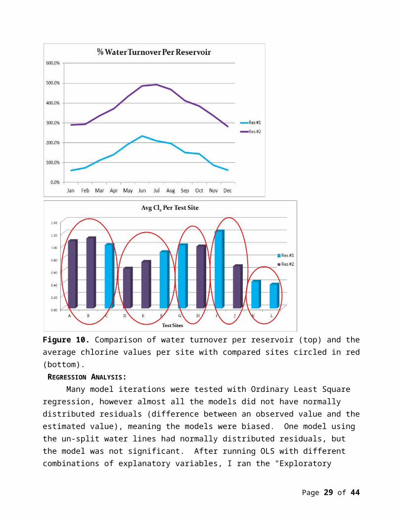
Figure 15. Interpolated surface using spring chlorine values

Page 29 of 34

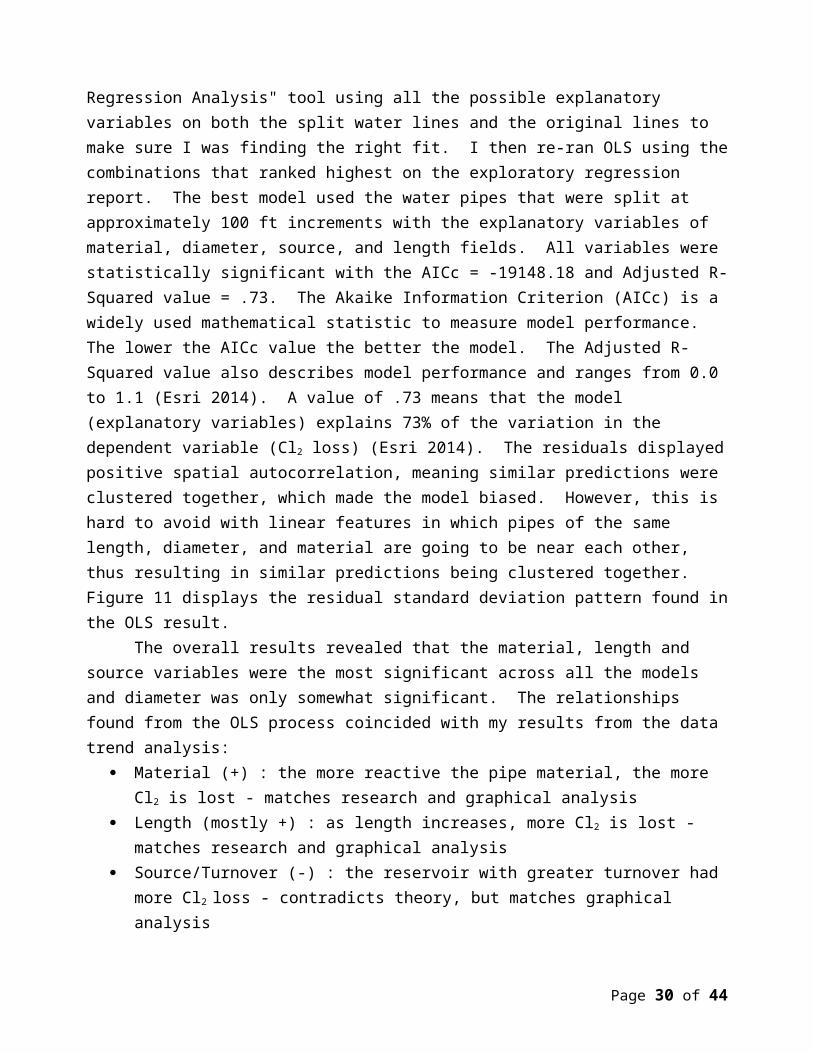
Figure 16. Interpolated surface created by combing the interpolation results from spring, summer, fall and winter Cl2 averages.

Page 30 of 34

CONCLUSIONS AND RECOMMENDATIONS The object of this study was to analyze the relationship of factors contributing to residual chlorine degradation and to determine if this approach could be used as a low cost alternative to model water quality factors without employing complex modeling software. Provided that, I have outlined the following conclusions:

The analysis is best performed using data over several years to establish a “normal” trend. As new Cl2 test are performed, cities can determine if the values are within predictable ranges. If values are way off, attention can be primarily focused on water usage changes (since distance, diameter & material would not have changed) or a possible hidden pipe break or leak that could be allowing contaminants into the system which would overwhelm the chlorine.

Using graphical analysis helps to support or interpret the results of statistical analysis and is an important part to determine if the model is reflecting the distribution system.

The greatest challenge to this or any analysis is the availability of data and ensuring that it is captured correctly in the GIS database. I was able to gather data about the system using engineering drawings, water usage from the utility department, and Cl2 values from the treatment plant and the testing organization. This is information that municipalities should have on hand and would need to be gathered by a hired consultant if they were to build the model.

There are two changes that I would recommend for the analysis methods:o I found that GWR was not significant in this analysis and could be easily left out. o Since water tests are performed 1-2 times per month or every other month, I think

it would have been better to obtain more frequent tests to ensure more accurate averages.

Overall, I would recommend this analysis to municipalities as a way to analyze their infrastructure as a whole and identify normal trends throughout the town. This analysis helps to raise awareness of factors within a distribution system that are not apparent by reading tables of Cl2 test values. The work also provides a visual interpretation of how the system is behaving and allows the operators to be more proactive by focusing on areas that need the most maintenance attention.

Page 31 of 34

Works CitedAl-Jasser, A.O. "Chlorine decay in drinking-water transmission and distribution systems: Pipe service age

effect." Water Research, 2007: 387-396.

Aqua. "Maintaining Disinfectant Residual in Distribution Systems." PA-AWWA Southeast District & Eastern Section WWOAP Spring Joint Conference. 2015.

AWWA; Economic and Engineering Services. Effects of Water Age on Distribution System Water Quality. Issue Paper, Environmental Protection Agency, 2002.

Bentley. Water Distribution Modeling and Analysis Software. n.d. https://www.bentley.com/en/products/product-line/hydraulics-and-hydrology-software/watercad?redirectPerm=true (accessed October 2015).

Centers for Disease Control and Prevention. The Safe Water System. July 17, 2014. http://www.cdc.gov/safewater/chlorine-residual-testing.html (accessed July 15, 2015).

—. The Safe Water System; Free Chlorine Testing. July 17, 2014. http://www.cdc.gov/safewater/chlorine-residual-testing.html (accessed October 21, 2015).

Childs, Colin. "Interpolating Sufaces in ArcGIS Spatial Analyst." ArcUser, 2004: 32-35.

DataStar. "StarTips, a resource for survey researchers." SurveyStar. n.d. http://www.surveystar.com/startips/jan2013.pdf (accessed July 17, 2015).

EPA. Basic Informaton about Disinfectants in Drinking Water: Chloramine, Chlorine, and Chlorine Dioxide. December 13, 2013. http://water.epa.gov/drink/contaminants/basicinformation/disinfectants.cfm (accessed October 15, 2015).

EPANET. EPANET Software that Models the Hydraulic and Water Quality Behavior of Water Distribution Piping Systems. August 19, 2015. http://www2.epa.gov/water-research/epanet (accessed October 16, 2015).

Esri - GWR. Interpreting GWR Results. n.d. 2016 (accessed January 20, 2016).

Esri - Kriging. ArcGIS Help 10.1: Kriging (Spatial Analyst). n.d. http://resources.arcgis.com/en/help/main/10.1/index.html#//009z0000006n000000 (accessed July 9, 2015).

Esri. Diffusion Interpolation With Barriers (Geostatistical Analyst). March 7, 2014. http://resources.arcgis.com/EN/HELP/MAIN/10.2/index.html#//003000000005000000 (accessed October 21, 2015).

—. Incremental Spatial Autocorrelation. n.d. http://desktop.arcgis.com/en/arcmap/10.3/tools/spatial-statistics-toolbox/incremental-spatial-autocorrelation.htm (accessed April 2016).

Page 32 of 34

—. Regression Analysis Basics. April 18, 2013. http://resources.arcgis.com/EN/HELP/MAIN/10.1/index.html#//005p00000023000000 (accessed October 21, 2015).

—. Understanding Path Distance Analysis. June 29, 2011. http://help.arcgis.com/EN/arcgisdesktop/10.0/help/index.html#/Understanding_path_distance_analysis/009z00000022000000/ (accessed October 21, 2015).

Goyal, Roopali V., and H.M. Patel. "Analysis of residual chlorine in simple drinking water distribution system with intermittent water supply." Applied Water Science, 2015: 311-319.

Haas, Charles N. "Benefits of Using a Disinfectant Residual." American Water Works Association, 1999: 65-69.

Hallman, N.B., J.R. West, C.F. Forster, J.C. Powell, and I. Spencer. "The decay of chlorine associated with the pipe wall in water distribution systems." Water Research, 2002: 3479-3488.

Hamdy, Diaa, Medhat A. E. Moustafa, and Walid Elbakri. "Free Residual Chlorine Calibration by WaterCAD at El-Nozha Water Network in Alexandria Governorate, Egypt." Journal of Environmental Protection, 2014: 845-861.

Innovyze. The Most Comprehensive Geospatial Water Distribution Modeling and Management Solution for ArcGIS. 2015. http://www.innovyze.com/products/infowater/ (accessed October 16, 2015).

Masters, Sheldon, Hong Wang, Amy Pruden, and Marc A. Edwards. "Redox Gradients in Distribution Systems Influence Water Quality, Corrosion, and Microbial Ecology." Water Research, 2015: 140-149.

Monteiro, L., et al. "Modeling of chlorine decay in drinking water supply systems using EPANET MSX." Science Direct, 2014: 1192-1200.

Mounce, Stephen Robert, Rebecca Sharpe, Vanessa Speight, Barrie Holden, and Joby Boxall. "Self-Organizing Maps for Knowledge Discovery from Corporate Databases to Develop Risk Based Prioritization for Stagnation." International Conference on Hydroinformatics. New York City: CUNY Academic Works, 2014.

Ray, Rajan, Laura Jacobsen, and Jerry Edwards. "Committee Report: Trends in water distribution system modeling." Journal AWWA, 2014: 51-59.

Rossman, Lewis A. EPANET 2 User Manual. Cincinnati, September 2000.

rssWeather. Climate for Las Vegas, Nevada. n.d. http://www.rssweather.com/climate/Nevada/Las%20Vegas/ (accessed July 15, 2015).

The Engineering Toolbox. Water Delivery Flow Velocities. n.d. http://www.engineeringtoolbox.com/pump-delivery-flow-velocity-water-d_232.html (accessed October 29, 2015).

Page 33 of 34

Turgeon, Steve, Manuel Rodriguez, Marius Theriault, and Patrick Levallois. "Perceptions of drinking water in the Quebec City region (Canada): the influence of water quality and consumer location in the distribution system." Journal of Environmental Management 70, 2004: 363-373.

Wang, Hong, et al. "Effect of Disinfectant, Water Age, and Pipe Material on Occurence and Persistence of Legionella, mycobacteria, Pseudomonas aeruginosa, and Two Amoebas." Environmental Science and Technology, 2012: 11566-11574.

Wang, Z. Michael, Hugh A. Devine, Weidong Zhang, and Kenneth Waldroup. "Using a GIS and GIS-Assisted Water Quality Model to Analyze the Deterministic Factors for Lead and Copper Corrosion in Drinking Water Distribution Systems." Journal of Environmental Engineering, 2014.

Water Quality and Health Council. Safe Water Delivered Safely. n.d. http://www.waterandhealth.org/drinkingwater/safewater.html (accessed November 1, 2015).

Page 34 of 34