Embed Size (px)
Citation preview
DOCUMENTOS DE ECONOMIA YFINANZAS INTERNACIONALES
Asociación Española de Economía y Finanzas Internacionales
http://www.fedea.es/hojas/publicaciones.html
ISSN 1696-6376
Las opiniones contenidas en los Documentos de la Serie DEFI, reflejan exclusivamentelas de los autores y no necesariamente las de FEDEA.
The opinions in the DEFI Series are the responsibility of the authors an therefore,do not necessarily coincide with those of the FEDEA.
Paths of Development in Open Economies:The Role of Land
María Dolores GuillóFidel Perez-Sebastian
March 2005
DEFI 05/04
Paths of Development in Open Economies:The Role of Land
María Dolores Guilló∗
[email protected] Perez-Sebastian∗
March 2005
Abstract
This paper shows, within a Heckscher-Ohlin version of the two-sector neo-classical growth model, that land, besides having long-run effects, is also a maindeterminant of the speed of convergence toward the steady state when thereare cross-sector capital share differences. This result stands in sharp contrastto the predictions of standard neoclassical growth frameworks, and calls for areinterpretation of the conditional-convergence and the resource-curse findings.More specifically, the model predicts that the former finding requires the exis-tence not only of diminishing returns but also of relatively small differences incapital shares across sectors. With respect to the latter finding, our results im-ply that it may be a consequence of purely transitional effects of natural richeson growth, and that it can not be interpreted as evidence that natural inputsnecessarily harm long-run welfare. We produce empirical evidence on the re-lationship between land, income levels, and growth rates, and present data oncross-sector capital shares. We claim that most of that evidence is consistentwith the predictions of the model.
JEL Classification: O41, F43.
∗Postal address: Universidad de Alicante, Departamento de Fundamentos del Análisis Económico,Campus de San Vicente s/n, 03690 Alicante, Spain. We thank the European Commission throughFEDER funds and the Spanish Ministry of Science and Technology, SEJ2004-08011ECON, and theInstituto Valenciano de Investigaciones Económicas, IVIE6-03I, for financial support.
1 Introduction
Standard neoclassical growth models imply that differences in labor productivities
affect only the position of a country along the development process. In other words,
they predict that country-specific factors not related to “deep” parameters have only
long-run effects with no influence on the speed of convergence. In sharp contrast to
these predictions, this paper shows, within an open-economy version of the two-sector
neoclassical growth framework, that a country’s relative land endowment, besides
having a long-run effect, is also a main determinant of the speed of convergence when
there are cross-sector capital share differences. Furthermore, the long-run effect and
the transitional effect of land can go in opposite directions. As a consequence, if two
economies start with the same income level but have different land endowments, the
economy that approaches a balanced-growth path with larger income levels can show
lower average growth rates along most of the transition path.
Besides the theoretical appeal, these results are interesting because they call for
a reinterpretation of two of the main empirical regularities about post-WWII cross-
country economic growth: the conditional convergence and the resource curse find-
ings. Barro (1991) shows that, after controlling for differences in long-run income
levels, poorer economies tend to grow faster than richer ones. That is, he finds condi-
tional convergence in the cross section of nations. The main theoretical explanation
for this empirical regularity comes from the standard neoclassical growth framework.
Which establishes that, if the degree of economic integration across nations is low, di-
minishing returns over accumulable inputs generate a decreasing income growth-rate
path as economies approach their long-run income levels. Our model predictions, on
the other hand, tell that the existence of diminishing returns are necessary, but may
not be sufficient to explain the evidence in favor of conditional convergence found in
the literature. The model implies that the conditional convergence finding requires
as well the existence of production technologies that exhibit capital shares that do
not vary much across activities.
Another important regularity affected by our model results is that natural-resources
usually appear as a curse in the cross section of countries. In particular, Sachs and
Warner (2001), among others, find that natural riches tend to slow down rather than
promote economic growth.1 Most current explanations for the curse have a crowding-
1Sala-i-Martin (1997) and Doppelhofer et al. (2004), however, find some contradictory results.
1
out logic. For example, Matsuyama (1992) and Galor and Mountford (2004) empha-
size that a larger natural endowment can reduce the incentives to allocate resources
to more growth-enhancing activities such as manufacturing and education, generat-
ing permanent differences in growth rates across countries. Most explanations then
interpret the finding as evidence that natural resources harm growth and long-run
income. We show that this does not need to be the case, because the empirical finding
might be capturing just a transitional effect. In our model, natural riches can be a
short-run curse for growth but a long-run blessing for income.
Our setup is similar to Atkeson and Kehoe’s (2000). The economy is composed of
a large number of small open economies. Each country has the production structure
of the standard two-sector neoclassical growth model with consumption and invest-
ment goods, extended to include land as a specific factor in the consumption sector.
The two sectors can have different input intensities. All Nations posses identical
preferences and production technologies, but they may differ regarding their land
endowment. Some countries, the developed world, have already reached their steady
states, while other countries begin to develop.
In the model, cross-sector differences in labor elasticities drive the effect of land on
steady-state income, whereas differences across sectors in capital-input shares drive
the land impact on the convergence speed. In particular, a larger land endowment
leads to higher long-run welfare levels if the investment-goods are more capital inten-
sive. However, if the consumption-goods sector is relatively labor intensive, a larger
stock of land has such a negative influence on capital accumulation that leads the
economy to permanently lower income. The model also predicts that land speeds
up convergence if investment goods are relatively capital intensive; land reduces the
speed of convergence otherwise. These pervasive negative effects of land only arise if
the economy transfers resources from one sector to the other, and their capital shares
differ. When the economy specializes in production, or capital shares are the same, it
behaves as a one-sector model in the sense that steady-state output always increases
with land, and the speed of convergence is independent of the natural stock.
An additional interesting result is that the model with land prevents a developing
economy from remaining permanently poorer than a developed country with the same
Consistent with the resource curse finding, they estimate a significant negative correlation betweenthe fraction of primary exports on total exports and growth. But, at the same time, they find astrong positive association between the fraction of GDP in Mining and growth.
2
land endowment. This is in contrast to the predictions of the standard dynamic
two-sector Heckscher-Ohlin model. In particular, Atkeson and Kehoe (2000) show
that, in this last framework, developing countries that are identical to developed
nations in all aspects except for the capital stock remain permanently poorer. The
difference between the two models is due to the uniqueness of the aggregate capital-
labor ratio compatible with a given return to capital in the model with land. More
specifically, when the return to capital has converged across economies, different
capital-labor ratios and income per capita levels are possible in the standard two-
sector model through cross-sector input movements. However, the specificity of land
to one industry implies that only one capital-labor ratio can accommodate the long-
run rental rate on capital in our framework, thus making differences in steady-state
income levels between identical economies impossible.
Other related papers that present models of international trade and growth are
Ventura (1997) and Mountford (1998).2 They use more or less standard two-sector
neoclassical growth models. Our model shares with them that the main results are
driven by the flow of resources across domestic sectors. Flow that in open economies
is not constrained by potentially low elasticities of domestic demand, because world
markets are assumed to be relatively large. However, they do not consider industry-
specific inputs.
As us, Ventura (1997) reinterprets the conditional convergence finding. He shows
that one can not use the conditional convergence result as sole evidence of diminishing
returns. He finds that when economies are integrated and factor prices per efficiency
unit are equalized across countries, diminishing returns are not sufficient to guarantee
conditional convergence among nations. In his model, besides diminishing returns,
it is necessary a sufficiently large elasticity of substitution between capital and labor
to make poorer countries grow faster than rich ones, holding constant differences
in labor productivity. Unlike him, we use Cobb-Douglas production functions with
a unitary elasticity of substitution, and maintain the international relative price of
2Within closed-economy scenarios, recent literature such as Caselli and Coleman (2001), Galor,Moav and Vollrath (2005), and Gollin, Parente and Rogerson (2002a,b) have already emphasizedthe importance of land in the growth and development process of real economies. Land is a peculiarproduction factor because is non-mobile, its supply is fixed, and its use is specific to some sectorssuch as agriculture. Exploiting these peculiar characteristics, the above papers propose land as amain determinant of the industrialization-process take-off, and cross-country labor-productivity andincome differences. Other papers include Kögel and Prskawetz (2001), Hansen and Prescott (2002),and Restuccia, Yang and Zhu (2004).
3
goods constant. In this way, we guarantee that the forces that drive Ventura’s (1997)
results are absent in our model.
The paper provides as well empirical evidence in favor of the model’s main predic-
tion that a country’s relative land endowment can have a significant transitional effect
on growth. In particular, we follow the method proposed by Mankiw, Romer and
Weil (1990) (MRW), and run steady-state level and growth regressions. We consider
a cross-section of 85 nations for the period 1967 to 1996. We find the typical MRW
result that investment rates, average educational attainment, and population growth
rates can explain about 76% of the cross-country output variance, with no improve-
ment when we introduce land. However, in the growth regression, the introduction of
land significantly improves the explanatory power of the regression. More specifically,
the estimates reveal that land has a negative impact on the convergence speed. This
is consistent with our model if consumption-goods production has a larger capital
elasticity than investment-goods manufacturing. We provide data on capital shares,
and claim that the evidence supports this view, even though the growth literature
has typically assumed the opposite.
The rest of the paper is organized as follows. Section 2 describes the economic
environment. Section 3 studies the developed-world’s diversified production equilib-
rium. Sections 4 analyzes the effect of a nation’s land endowment on its development
path. A numerical exploration of the model predictions is carried out in section 5.
Section 6 presents the empirical evidence. Section 7 concludes.
2 The Economy
Consider a world economy consisting of a large number of small open economies that
differ only in their land input endowment and in their level of development. There are
two goods, and three inputs of production. The production of the consumption and
the investment goods needs capital and labor inputs, which can freely move across
sectors. In addition, the consumption-goods sector uses a specific factor, land. There
is free trade in goods, but international movements of inputs are prohibited. All
markets are perfectly competitive. Population is constant and its size equals L.
Infinitely-lived consumers discount future utility with the factor ρ, and have pref-
4
erences only over consumption. In particular, their preferences are given by
∞Xt=0
ρtµc1−σt − 11− σ
¶, ρ ∈ (0, 1) , σ > 0. (1)
Individuals offer labor services and rent capital and land to firms. The total amount
of land in the economy is fixed over time, equals N , and is uniformly distributed
across all individuals. Since in each period international trade must be balanced,
consumers in each country face the following budget constraint
ct + ptxt = rktkt + rntnt + wt, (2)
where the evolution of capital is governed by
kt+1 = (1− δ) kt + xt. (3)
In the above expressions, ct is the per capita demand for consumption goods; xt is
the per capita demand for investment goods, whose price is pt; rkt, rnt, and wt are,
respectively, the rental rates on capital, land, and labor; nt and kt denote the amount
of the natural input and capital own by the individual at date t, respectively. The
consumption good is the numeraire.
Consumers in each country will maximize (1) subject to (2) and (3), taking as
given the world output prices and the domestic rental rates for production factors.
The Euler equation corresponding to this dynamic programing problem is
ct+1ct
=
·pt+1pt
ρ
µrkt+1pt+1
+ 1− δ
¶¸1/σ. (4)
It is standard. It says that the growth rate of consumption depends on the present-
utility value of the rate of return to saving. This return reflects that giving up a
unit of present consumption allows today buying 1/pt units of the investment good
that, after contributing to the production process, will covert themselves tomorrow
in 1 + rkt+1/pt+1 − δ units that can be sold at a price pt+1.
In each nation, production of the consumption good (Yct) is given by
Yct = AKαctN
βL1−α−βct = ALctkαctn
βct, α, β ∈ (0, 1) . (5)
And manufacturing of the investment good (Yxt) by
Yxt = BKθxtL
1−θxt = BLxtk
θxt, θ ∈ (0, 1) . (6)
5
Above, Kit and Lit denote, respectively, the amount of capital and labor devoted in
period t to the production of good i; and nct = N/Lct, kit = Kit/Lit, for all i = c, x.
Denote the labor share in the production of good i by lit = Lit/L. Notice that
because consumers are alike, the amount of capital own by each individual will equal
the country’s capital-labor ratio. Hence, the constraints on labor and capital within
a country can be written as follows:
lct + lxt = 1, (7)
lctkct + lxtkxt = kt. (8)
Firms in each country will maximize profits taking as given world prices and the
domestic rental rates on production factors. From the production functions (5) and
(6), and assuming that capital and labor can freely move across sectors, production
efficiency implies that
rkt = αAkα−1ct nβct = ptθBkθ−1xt , (9)
rnt = βAkαctnβ−1ct , (10)
wt = (1− α− β)Akαctnβct = (1− θ) ptBk
θxt. (11)
Of course, these equalities will hold only for the technologies that coexist in
equilibrium. The following two results establish the firms that open in equilibrium.3
Proposition 1 For any wage rate wt and capital rental rate rkt, it is profitable to
operate the consumption technology.
Proposition 2 Domestic firms will enter the investment-goods market if and only if
pt >A
B
³αθ
´θ µ1− α− β
1− θ
¶1−θnβ kα−θt ; (12)
where n = N/L; and pt and kt denote equilibrium values when only consumption
goods are produced in the domestic economy.
The right side of expression (12) determines a minimum price above which it be-
comes profitable for investment-goods producers to enter the market. This minimum
price depends on the relative endowment of land, the stock of capital per capita,
3The proofs of the propositions presented in the paper are contained in appendix A.
6
and factor intensities, let us denote it by pmin(kt;n). An small open economy then
specializes in the production of c goods if pmin(kt;n) is greater than or equal to the
international price pt. More specifically, closing the investment-products sector be-
comes more appealing as n increases and as pt declines or, in other words, as the
consumption-goods activity becomes relatively more productive for given kt. Larger
values of kt have the same effect as larger stocks of n when the share of capital is
greater in the consumption sector, but they have the opposite effect when the share
of capital is larger in the investment sector. In addition, notice that under diversifi-
cation, pmin(kct;nct) must equal the international price level pt at every point in time
t for the market-equilibrium zero-profit condition to hold, a property that will prove
helpful in our analysis.
We conclude that consumption items will always be supplied by domestic pro-
ducers because they require a specific factor that is in positive supply. The economy,
however, may not manufacture investment goods. This will depend on prices, and on
the economy’s endowments of land and capital relative to labor.
3 The Developed-World’s Diversified-Production Equi-librium
Suppose that all but one of these countries have already reached the steady-state. We
can think of this group of nations as the developed world. In addition, assume that
all developed countries share the same endowments. Next, we study the steady-state
allocations of the developed world.
In equilibrium, identical countries make the same choices. So the equilibrium for
this developed world economy will be the same as the equilibrium for a single large
and closed economy, and it will not be affected by the behavior of the small (still
developing) country. Therefore, we can write the world market clearing conditions
for final goods as
ct = Alctkαctn
βct, (13)
xt = Blxtkθxt. (14)
In equilibrium, the world economy will produce positive amounts of both goods.
Define the relative factor price ωkt = wt/rkt. The efficiency conditions in production
(9) and (11) determine the optimal allocations of capital as a function of the relative
7
factor price:
kxt =
µθ
1− θ
¶ωkt, (15)
kct =
µα
1− α− β
¶ωkt, (16)
It follows from (15) and (16) that consumption goods will be more capital intensive
if and only if θ (1− β) < α, and that kct > kxt if α > θ. We next determine the labor
allocations. Equations (9), (15) and (16) imply
lct = n
"Aαα (1− α− β)1−α
Bθθ (1− θ)1−θ
Ãωα−θkt
pt
!# 1β
. (17)
The labor share lct depends negatively on the relative output price and positively
on the per capita amount of land. The labor share is also affected by the relative
input price of labor to capital, but the effect of this price on lct will depend on the
relative capital shares across sectors. The effect will be positive if α > θ, and negative
otherwise. From (17), we can obtain as a residual the labor allocation lxt, using the
economy’s labor constraint (expression (7)).
Let us now focus on the steady-state equilibrium path. Over there, variables in
per capita terms, relative employment of inputs and prices will remain invariant. De-
noting by an asterisk (∗) steady-state outcomes, the consumers’ optimality condition(4) implies
r∗k = p∗£ρ−1 + δ − 1¤ . (18)
The interest rate in terms of investment goods at steady state is exclusively pin down
by consumers’ preferences.
Using the expression for r∗k and condition (9), we obtain the steady state capital-
labor ratio in investment-goods production:
k∗x =µ
θB
ρ−1 + δ − 1¶ 1
1−θ. (19)
Equations (15), (16), (18) and (19) determine the values of the relative factor prices
and the capital-labor ratio in the consumption-goods sector at the steady state equi-
librium. Notice that, at the world’s diversified-production equilibrium, the steady
state capital-labor ratios do not depend on the natural resource endowment. This
8
occurs because kc and kx are a function of factor intensities and the relative fac-
tor price ωkt, but at the steady state ω∗k is exclusively determined by consumers’
preferences and factor intensities in the x sector.
The aggregate stock of capital in the economy can be derived from equations (3),
(9), (14) and (18). At steady-state,
k∗ =µρ−1 + δ − 1
θδ
¶l∗xk
∗x. (20)
Clearly, the stock of capital must be completely split among its different uses given,
in relative terms, by equation (8). This market-equilibrium condition determines p∗.
More specifically, combining equations (7), (8), (15), (16), (17), (19) and (20), we
obtain
p∗ =
³1−α−β1−θ
´1−α ¡αθ
¢αBA
³θB
ρ−1+δ−1´ θ−α1−θ
½1 +
αδ (1− θ)
(1− α− β) [ρ−1 + δ (1− θ)− 1]¾β
nβ. (21)
The result is quite intuitive. As c production becomes more profitable than x man-
ufacturing because land is more abundant, the economy devotes relatively more re-
sources to the production of consumption goods, making investment products rela-
tively scarcer and, as a consequence, more expensive.
Another important variable that we are particularly interested in is aggregate
output, defined as the weighted sum of consumption- and investment-goods produc-
tion,
yt = lctyct + ptlxtyxt. (22)
Using expressions (5) to (7), (9), (15) and (16), and taking into account that ωkt =
wt/rkt, we can write a developed nation’s GDP level per capita as
yt =wt
1− θ
·1 + lct
µα+ β − θ
1− α− β
¶¸. (23)
It is interesting to note that the economy’s GDP can decrease with a larger alloca-
tion of labor into the production of consumption items if this activity is more labor
intensive than investment-goods manufacturing. From expression (23), we can use
(15), (17) to (19), and (21) to obtain y∗.
We have derived the equations that characterize the diversified equilibrium, and
obtained the steady-state for the developed world. Next, we focus on the adjustment
paths implied by the model for developing nations.
9
4 Development Paths
Consider now the other small nation that is still moving along its adjustment path
and suppose that it has initially a capital stock k0 < min {k∗c , k∗x}. We can think ofthis late-blooming nation as a developing country that faces the steady-state relative
output price obtained above for the developed world — i.e., pt = p∗ for all t. From
here on, the asterisk (∗) denotes the international diversified-production equilibriumfor the world economy, whereas we remove the time subscript to denote the steady
state values for the initially less developed country. The next proposition describes
the initial pattern of production of the latter economy.
Proposition 3 Let kd be the value that solves the equation p∗ = pmin(kd;n). In
particular,
kd = k∗c · n/n∗
1 + αδ(1−θ)(1−α−β)(ρ−1+δ(1−θ)−1)
β/(θ−α)
. (24)
A less developed country with a land/labor endowment equal to n and with an initial
capital/labor ratio given by k0 will initially diversify production if k0 > kd for α < θ,
or if k0 < kd for α > θ. It will specialize in consumption-goods production otherwise.
Let us now study, separately, the development paths for each of the two possible
initial scenarios: specialization and diversification.
4.1 The diversified-production case
Suppose first that θ > α. As stated in Proposition 3, the late-bloomer starts its
development path diversifying production if ko > kd. In this case it continues to
produce both goods at all times in the future since its pmint decreases with kt and
the world price is fixed at p∗. That is, it will diversify production and accumulate
capital until its rental rate falls down to the world’s rate r∗k, which is by equation
(18) exclusively determined by consumers’ preferences and p∗. Next, notice that
equations (15) to (19) describe the behavior of all our economies, regardless of their
resource endowment, as long as they lie within the diversification cone. Therefore,
at the steady state, expressions (15) to (19) imply that kx = k∗x, ωk = ω∗k, and
kc = k∗c . And from expressions (9) to (11), nc = n∗c , rn = r∗n, and w = w∗. In sum,
in the long run, factor-price equalization will hold, and the country will be using the
same techniques as the rest of developed nations. Notice that we obtain factor-price
10
equalization because the x-goods technology only uses mobile-factors, and pins down
the relative factor prices for the whole economy.
Suppose now that θ < α. In this case, at the world’s diversified production
equilibrium, we have that k∗x < k∗ < k∗c , and the late-bloomer starts its development
path diversifying production if ko < kd. Now pmint increases with kt and so switching
to specialization cannot, in principle, be ruled out. However, taking into account
that ko < k∗x, it is easy to show that diversification will continue at all times in the
future whenever its land/labor endowment n is not too large relative to n∗. To see
this, note that under these conditions expression (24) implies that kd > k∗c .
The difference with the world economy will come regarding the overall capital
stock of the developing nation and the labor allocations. Notice that the equality
nc = n∗c implies that a lower endowment of land will make optimal to allocate a lower
fraction of labor to consumption-goods production. That is, if n is lower than the
devoloped world’s average n∗, then lc < l∗c . In that case, expressions (8), (15) and
(16) evaluated at the steady state, imply that k > k∗ if θ > α/(1− β), and k < k∗ if
θ < α/(1 − β). On the other side, if n is greater than n∗, we have that lc > l∗c and
the opposite effects follows for k. That is, a relatively land-abundant nation achieves
a steady-state stock of capital that is larger (smaller) than the world’s average if
consumption-goods are relatively more (less) capital intensive.
The next proposition summarizes the main results.
Proposition 4 Suppose a small late-blooming nation with k0 < min {k∗c , k∗x} thatstarts its development process producing positive amounts of both goods. Then, for all
kc and kx, it stays in a diversified-production equilibrium at all times and accumulates
capital until factor-price equalization holds if α < θ. But if α > θ, then it will
diversify production in the long run only if n/n∗ is not too large. Under a diversified
production equilibrium, the country’s steady-state income y will decrease with n if
the share of labor in consumption-goods production is larger than in investment-goods
manufacturing; y will increase with n otherwise.
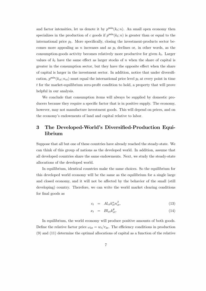
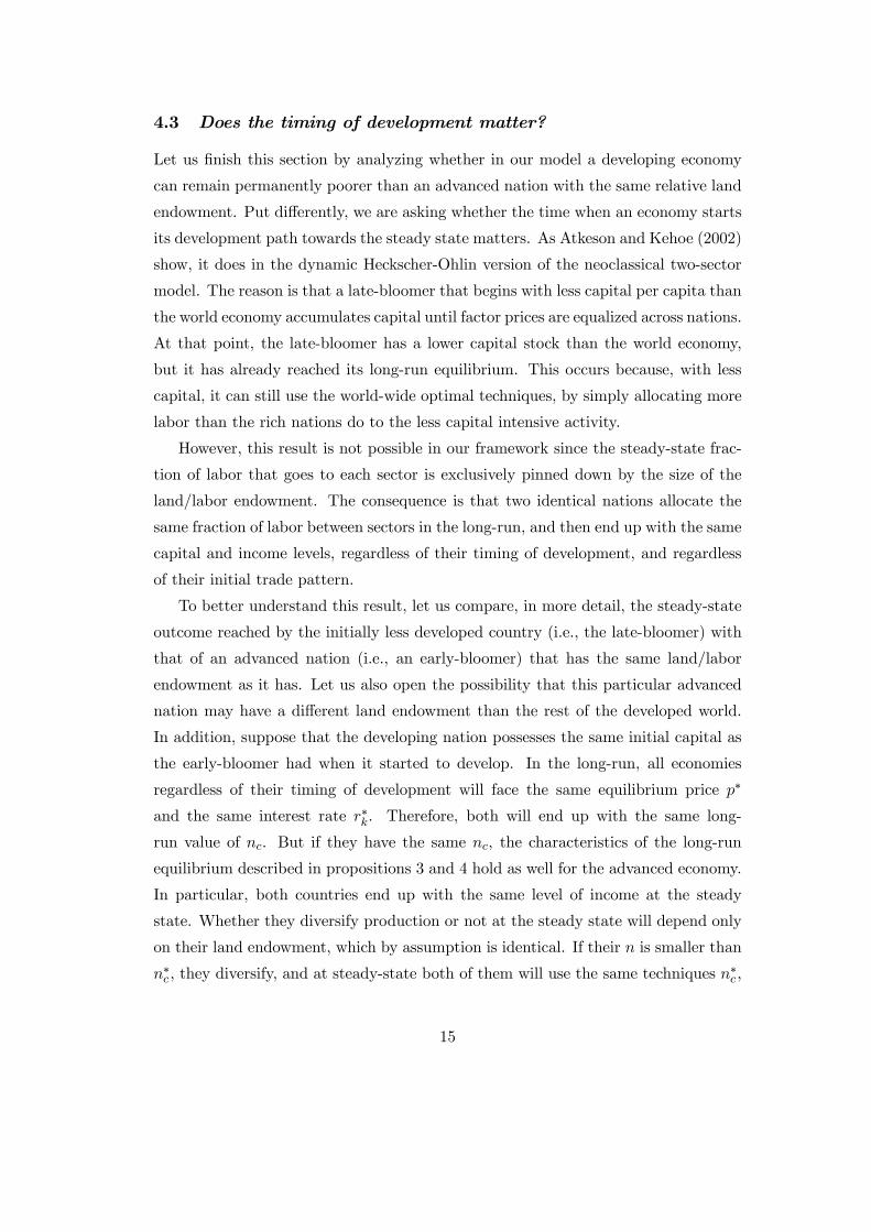
Figure 1 illustrates the above development paths. It shows the phase diagram
of the dynamic system in the plane (k, c), for given n, for the developing nation,
assuming that α < θ. The CC schedule represents the Euler equation for consumption
when c is stationary. From equations (4), (7) to (9), (15) and (16), we have that the
11
CC line represents
ct+1 − ctct
= ρ1σ
"θB
µθ
1− θ
¶θ−1ωθ−1kt + 1− δ
# 1σ
− 1 = 0; (25)
where ωkt is implicitly given by
p∗ =
nωα−θβ
kt
(1−α−β)(1−θ)α−θ(1−β)
³ktωkt− θ
1−θ´β Aαα(1− α− β)1−α
Bθθ(1− θ)1−θ. (26)
The KK schedule comes from the capital motion equation, expression (3), when
this variable is stationary, and is composed of two different pieces. To the left of kd,
the economy specializes and then investment equals p∗xt = yct − ct. To the right of
kd, the economy diversifies and p∗xt = yt − ct. With diversification, the line is less
concave because the reallocation of resources between sectors ameliorates the effect
of diminishing returns to capital accumulation. From equations (3), (5) to (8), (11),
(15) and (23), the KK line is given by
kt+1 − kt =
µyt − ctp∗
¶− δkt = 0; (27)
where
yt = Akαt nβ if kt ≤ kd;
= p∗Bµ
θ
1− θ
¶θ
ωθkt
·1 +
(α+ β − θ)(1− θ)
α− θ(1− β)
µktωkt− θ
1− θ
¶¸if kt > kd.
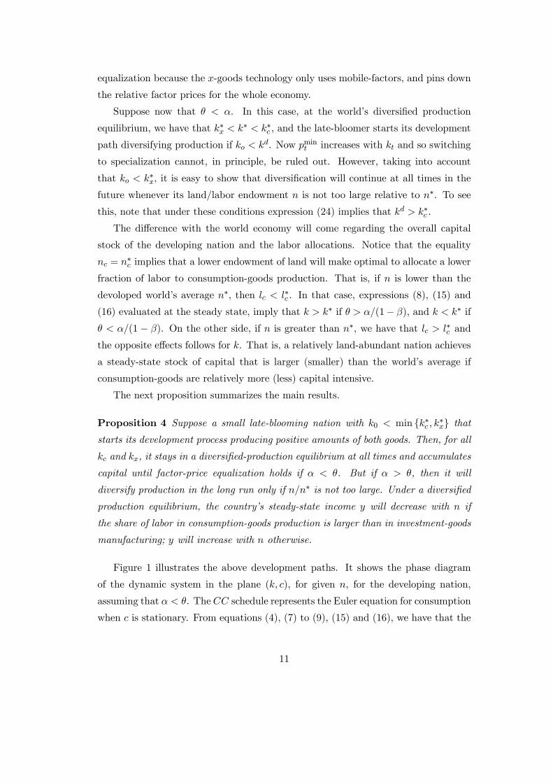
The phase diagram in Figure 1 looks very much like the one in a standard Cass-
Koopmans one-sector model. In our case, the steady state solution depends on
the value of n. Assuming that investment goods are more capital intensive (i.e.,
θ (1− β) > α), an increase in n will shift the curve KK upwards and the curve
CC to the left. To understand the last statement, note that an increase in n will
increase income for any given capital, so consumption must rise to control the flow of
investment and keep capital stationary (the curve KK shifts upwards). Similarly, an
increase in n implies an increase in the share of labor allocated to the consumption
sector to keep marginal productivity at the steady-state interest rate level. This, in
turn, requires a lower stock of capital for any given level of consumption (the CC
locus shifts to the left). As a result of these shifts, the new steady state levels of
capital and consumption could be above or below the former ones. We know that the
12
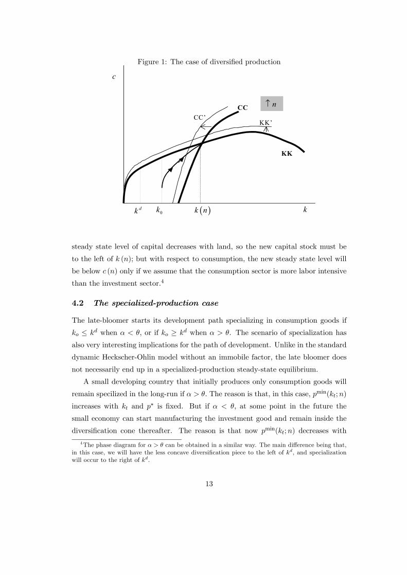
Figure 1: The case of diversified production
KK
CC
( )k n k
c
dk 0k
CC’KK’
n↑
steady state level of capital decreases with land, so the new capital stock must be
to the left of k (n); but with respect to consumption, the new steady state level will
be below c (n) only if we assume that the consumption sector is more labor intensive
than the investment sector.4
4.2 The specialized-production case
The late-bloomer starts its development path specializing in consumption goods if
ko ≤ kd when α < θ, or if ko ≥ kd when α > θ. The scenario of specialization has
also very interesting implications for the path of development. Unlike in the standard
dynamic Heckscher-Ohlin model without an immobile factor, the late bloomer does
not necessarily end up in a specialized-production steady-state equilibrium.
A small developing country that initially produces only consumption goods will
remain specilized in the long-run if α > θ. The reason is that, in this case, pmin(kt;n)
increases with kt and p∗ is fixed. But if α < θ, at some point in the future the
small economy can start manufacturing the investment good and remain inside the
diversification cone thereafter. The reason is that now pmin(kt;n) decreases with
4The phase diagram for α > θ can be obtained in a similar way. The main difference being that,in this case, we will have the less concave diversification piece to the left of kd, and specializationwill occur to the right of kd.
13
kt and it becomes more likely that pmin falls below p∗. Nevertheless, whether the
developing country remains specialized in the long run will depend crucially on its
endowment of the specific factor relative to the developed world’s.
Consider the situation where the developing nation is specialized in the long run.
The economy accumulates capital through imports of investment goods, with kt = kct
and lct = 1 for all t, until the domestic rate of return on capital equals the world’s
rate, rk = r∗k. At that point, the firms’ efficiency condition (9), and the world’s
production techniques, n∗c and k∗c , imply that
k =
µn
n∗c
¶ β1−α
k∗c . (28)
For this specialized-production situation really to be an equilibrium for the late-
blooming country, it must be also true that domestic investment-goods firms do not
find profitable to operate. That is, that condition (12) does not hold when capital is
given by (28). Substituting (28) into (12), we can easily find that the late-bloomer
will never diversify production in the long run if its relative land endowment satisfies
n ≥ n∗c . (29)
If the nation converges to a specialized-production equilibrium, conditions (29)
and (28) imply that k ≥ k∗c . Note that this inequality implies that k > k∗ when
consumption goods are more capital intensive than investment goods. Moreover,
under specialization, both the long-run capital-labor ratio and income level are pos-
itively related to n, because an increase in land endowment can no longer induce a
resource stealing effect on other sectors. Therefore, for n sufficiently large, the spe-
cialized country can accumulate enough capital so that its long run level of income,
y = Anβkα, be above the developed world’s average.
Suppose now that condition (29) is not satisfied and that α < θ. Then, it follows
that the late-blooming economy with k0 ≤ kd will switch to diversified production at
some point in time t > 0, when kt is still smaller than its steady-state level. Once the
economy enters its diversification cone, it will stay there thereafter and the results
established in proposition 3 will hold.
Proposition 5 Suppose a small open-economy that initially specializes in consumption-
goods production. Then, specialization will persist in the long-run if α > θ or if α < θ
and n ≥ n∗c . Contrary to the diversified-production scenario, under specialization the
country’s long-run income per capita always rises with the land endowment.
14
4.3 Does the timing of development matter?
Let us finish this section by analyzing whether in our model a developing economy
can remain permanently poorer than an advanced nation with the same relative land
endowment. Put differently, we are asking whether the time when an economy starts
its development path towards the steady state matters. As Atkeson and Kehoe (2002)
show, it does in the dynamic Heckscher-Ohlin version of the neoclassical two-sector
model. The reason is that a late-bloomer that begins with less capital per capita than
the world economy accumulates capital until factor prices are equalized across nations.
At that point, the late-bloomer has a lower capital stock than the world economy,
but it has already reached its long-run equilibrium. This occurs because, with less
capital, it can still use the world-wide optimal techniques, by simply allocating more
labor than the rich nations do to the less capital intensive activity.
However, this result is not possible in our framework since the steady-state frac-
tion of labor that goes to each sector is exclusively pinned down by the size of the
land/labor endowment. The consequence is that two identical nations allocate the
same fraction of labor between sectors in the long-run, and then end up with the same
capital and income levels, regardless of their timing of development, and regardless
of their initial trade pattern.
To better understand this result, let us compare, in more detail, the steady-state
outcome reached by the initially less developed country (i.e., the late-bloomer) with
that of an advanced nation (i.e., an early-bloomer) that has the same land/labor
endowment as it has. Let us also open the possibility that this particular advanced
nation may have a different land endowment than the rest of the developed world.
In addition, suppose that the developing nation possesses the same initial capital as
the early-bloomer had when it started to develop. In the long-run, all economies
regardless of their timing of development will face the same equilibrium price p∗
and the same interest rate r∗k. Therefore, both will end up with the same long-
run value of nc. But if they have the same nc, the characteristics of the long-run
equilibrium described in propositions 3 and 4 hold as well for the advanced economy.
In particular, both countries end up with the same level of income at the steady
state. Whether they diversify production or not at the steady state will depend only
on their land endowment, which by assumption is identical. If their n is smaller than
n∗c , they diversify, and at steady-state both of them will use the same techniques n∗c ,
15
k∗c and k∗x. In addition, since n is fixed, the steady state fraction of labor devoted
to consumption-goods production lc will also be the same in both economies, and
therefore so will be the capital stock and income per capita. On the other hand, if
their n is larger than n∗c , they specialize; in that case, their steady-state capital is
given by (28) and we achieve the same conclusion. Put differently, in the long-run
the threshold level of capital kd that determines the production pattern (given by
(24) ) is the same for both countries.
The timing of development, however, does affect production patterns along the
adjustment path. The reason is that a late-bloomer and an early-bloomer face dif-
ferent world prices of goods at the time they start to develop. A late-bloomer faces
a constant price p∗at all times, whereas the early-bloomer faces a sequence of world
prices pt that converges to p∗. Therefore, the threshold level of capital that deter-
mines the production pattern of an early-bloomer when it starts to develop kdo (i.e.,
kdo is such that pmin(kd0 ;n) = p0) is different from its long-run level kd, which is the
same as the one that determines the late-bloomer’s initial pattern of production. For
instance, if the two countries diversify production in the long-run and α > θ, it must
be true that their common long-run stock of capital k is below kd. Then, k0 < k
implies that k0 < kd and so the late-bloomer diversifies production initially, but the
early-bloomer could have started diversifying or not since k0 can be below or above
kd0.
The next proposition summarizes these results.
Proposition 6 If two countries possess the same stock of land per capita, they con-
verge to the same long-run income per capita level, regardless of their timing of de-
velopment. However, their trade patterns may differ along the adjustment path.
5 Income Levels and Convergence Rates
Our next task is to conduct a numerical experiment to evaluate the possible impact of
a country’s relative land endowment on its steady-state level of output and speed of
convergence. After that, we will use this information to reinterpret the conditional-
convergence and resource-curse findings in terms of our model.
16
5.1 Calibration
In order to advance in that direction, we need to calibrate the model parameters. We
calibrate the parameters so that the steady state equilibrium of the developed world
is consistent with main US growth facts. We choose 0.95 for the discount factor ρ,
1 for the inverse of the intertemporal elasticity of consumption σ, and 0.08 for the
depreciation rate δ. These values are standard in the literature. In addition, we
normalize B equal to 1, and set p∗ equal to 0.64, the price of equipment relative to
consumption for the U.S. reported by Eaton and Kortum (2001). The developed-
world’s land-labor ratio n∗ is set equal to 1.69, the U.S. average for the period 1967
to 1996, obtained from the Food and Agriculture Organization (FAO) of the United
Nations.5
Regarding the production technology parameters, we do not have any available
estimates for the consumption and investment sectors. However, we do have infor-
mation about the shares of the different inputs in GDP. Parente and Prescott (2000)
report that a share of capital of 0.25, a land share of 0.05, and a labor share of
0.70 are consistent with the U.S. growth experience. In addition, we can obtain an
estimate of the sectoral composition of GDP employing investment shares. For the
period 1980 to 1990, the average investment share for the U.S. is 0.21. This number
implies a steady-state value for the share of investment-goods of
p∗y∗xl∗xy∗
=p∗δk∗
y∗= 0.21.
Hence, the one for consumption products is
y∗c l∗cy∗
= 0.79.
This sectoral composition and the share of capital for the whole U.S. economy deliver
the following relationship between the capital shares in the two production activities:
0.21θ + 0.79α = 0.25. (30)
In addition, the share of land in GDP requires that
β
µy∗c l∗cy∗
¶= 0.05 ⇒ β = 0.064. (31)
5Detailed description of the data used in the paper is provided in the data appendix.
17
In accordance with (30), we consider the following set of values for the capital
shares:
(α, θ) = {(0.21, 0.40), (0.24, 0.30), (0.25, 0.25), (0.27, 0.17), (0.29, 0.09)}.
5.2 Results
We compute, for a developing nation, its relative steady-state income level with
respect to the developed-world economy, and its speed of convergence for different
values of the land per worker endowment.
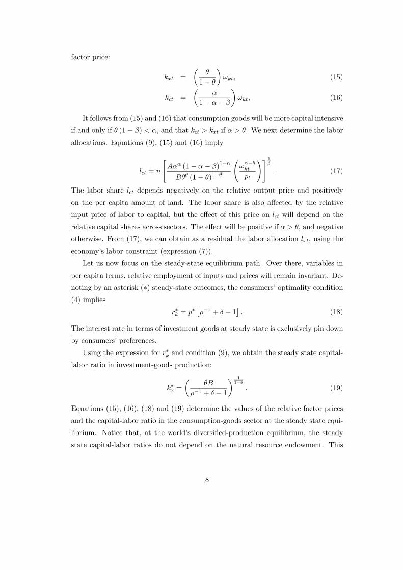
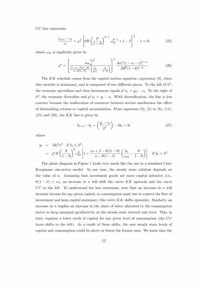
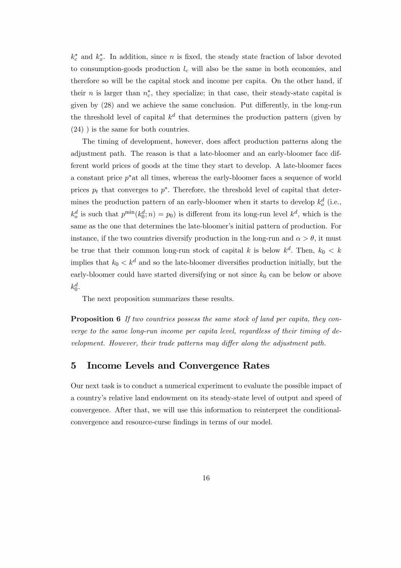
Figure 2 shows a country’s relative-income steady-state level as a function of
its land endowment for three sets of parameters. The domain of n is the interval
[0.002, 6.72] that contains all values of arable-land hectares per worker across nations
(averages for the period 1967-1996) in FAO statistics. It illustrates the relationship
already established in Propositions 3 and 4. When (α, θ) = (0.21, 0.40) (dotted line
in chart), the labor share in the consumption-goods sector is relatively larger than
the labor share in the investment-goods sector. As a consequence, long-run output in
diversified-production economies decline with n. Under diversification, the schedule
is linear because factor-price equalization holds and, then, equations (17) and (23)
define a linear relationship between y and n. Under specialization, on the other hand,
output equals Anβkα. Hence, equation (28) implies that the relationship between y
and n is strictly increasing and concave to the right of n∗c . When (α, θ) = (0.21, 0.40),
we observe that n∗c = 2.0. This value of n∗c implies that 95 percent of countries in
FAO statistics would be operating within the diversification cone.
In the intermediate case (solid line), (α, θ) = (0.24, 0.30), labor shares in both
activities are the same. The difference with respect to the previous case is that
now land does not affect output in economies that operate within the diversification
cone. The third scenario (dashed line), (α, θ) = (0.27, 0.18), depicts a bigger labor
share in the investment-goods sector. Thus, steady-state income always increases
with land. If we look at the numerical value of the predicted income differences, they
are significant although relatively small. For example, focusing in the last scenario,
the highest income level is only 36% bigger than the level predicted for the poorest
nation.
Next, we study the speed of convergence.6 Differences in the stock of land have a
6As previous literature, we linearize the equilibrium-dynamics system, given by expressions (25)
18
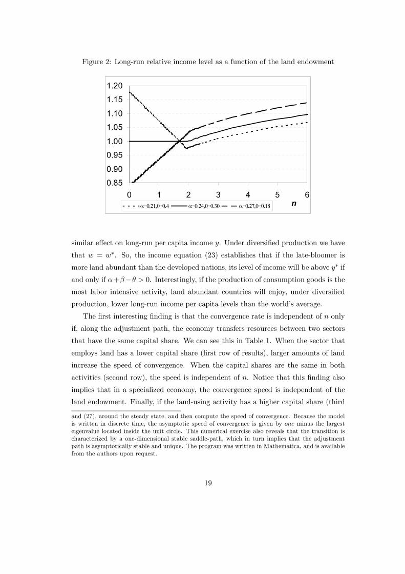
Figure 2: Long-run relative income level as a function of the land endowment
0.85
0.90
0.95
1.00
1.05
1.10
1.15
1.20
0 1 2 3 4 5 6nα=0.21,θ=0.4 α=0.24,θ=0.30 α=0.27,θ=0.18
similar effect on long-run per capita income y. Under diversified production we have
that w = w∗. So, the income equation (23) establishes that if the late-bloomer is
more land abundant than the developed nations, its level of income will be above y∗ if
and only if α+β−θ > 0. Interestingly, if the production of consumption goods is themost labor intensive activity, land abundant countries will enjoy, under diversified
production, lower long-run income per capita levels than the world’s average.
The first interesting finding is that the convergence rate is independent of n only
if, along the adjustment path, the economy transfers resources between two sectors
that have the same capital share. We can see this in Table 1. When the sector that
employs land has a lower capital share (first row of results), larger amounts of land
increase the speed of convergence. When the capital shares are the same in both
activities (second row), the speed is independent of n. Notice that this finding also
implies that in a specialized economy, the convergence speed is independent of the
land endowment. Finally, if the land-using activity has a higher capital share (third
and (27), around the steady state, and then compute the speed of convergence. Because the modelis written in discrete time, the asymptotic speed of convergence is given by one minus the largesteigenvalue located inside the unit circle. This numerical exercise also reveals that the transition ischaracterized by a one-dimensional stable saddle-path, which in turn implies that the adjustmentpath is asymptotically stable and unique. The program was written in Mathematica, and is availablefrom the authors upon request.
19
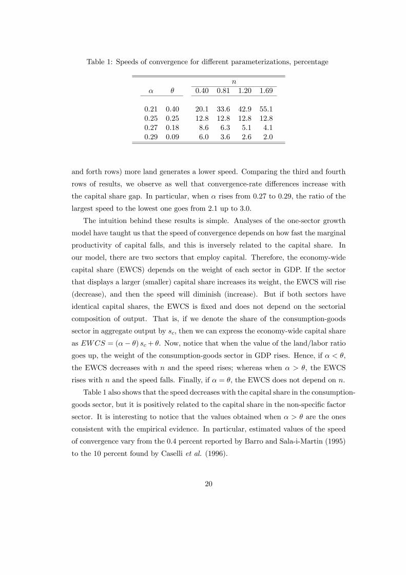
Table 1: Speeds of convergence for different parameterizations, percentage
nα θ 0.40 0.81 1.20 1.69
0.21 0.40 20.1 33.6 42.9 55.10.25 0.25 12.8 12.8 12.8 12.80.27 0.18 8.6 6.3 5.1 4.10.29 0.09 6.0 3.6 2.6 2.0
and forth rows) more land generates a lower speed. Comparing the third and fourth
rows of results, we observe as well that convergence-rate differences increase with
the capital share gap. In particular, when α rises from 0.27 to 0.29, the ratio of the
largest speed to the lowest one goes from 2.1 up to 3.0.
The intuition behind these results is simple. Analyses of the one-sector growth
model have taught us that the speed of convergence depends on how fast the marginal
productivity of capital falls, and this is inversely related to the capital share. In
our model, there are two sectors that employ capital. Therefore, the economy-wide
capital share (EWCS) depends on the weight of each sector in GDP. If the sector
that displays a larger (smaller) capital share increases its weight, the EWCS will rise
(decrease), and then the speed will diminish (increase). But if both sectors have
identical capital shares, the EWCS is fixed and does not depend on the sectorial
composition of output. That is, if we denote the share of the consumption-goods
sector in aggregate output by sc, then we can express the economy-wide capital share
as EWCS = (α− θ) sc + θ. Now, notice that when the value of the land/labor ratio
goes up, the weight of the consumption-goods sector in GDP rises. Hence, if α < θ,
the EWCS decreases with n and the speed rises; whereas when α > θ, the EWCS
rises with n and the speed falls. Finally, if α = θ, the EWCS does not depend on n.
Table 1 also shows that the speed decreases with the capital share in the consumption-
goods sector, but it is positively related to the capital share in the non-specific factor
sector. It is interesting to notice that the values obtained when α > θ are the ones
consistent with the empirical evidence. In particular, estimated values of the speed
of convergence vary from the 0.4 percent reported by Barro and Sala-i-Martin (1995)
to the 10 percent found by Caselli et al. (1996).
20
5.3 Reinterpreting the conditional convergence and resource cursefindings
Taken together, the above results on long-run income and on the speed of convergence
are very interesting. They say that, in sharp contrast to the predictions of the
standard neoclassical growth framework, our model implies that two nations that are
at the same distance of their specific steady-states do not necessarily converge at the
same speed. Furthermore, if capital shares in the two sectors are different and the
sector with the larger cpital share is also the less labor intensive, the country that
in the long-run becomes relatively richer converges at a lower speed than the nation
that in the long-run becomes poorer. The first statement has implications for the
interpretation of the conditional convergence evidence, whereas the second one does
it for the resource curse finding.
To improve our understanding of the potential effects of land and cross-sector
capital-share differences on the interpretation of these two empirical regularities, let
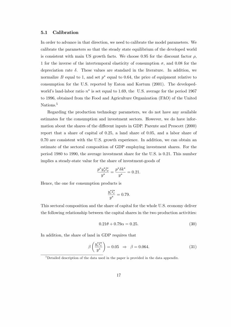
us focus on the (α, θ) = (0.29, 0.09) scenario, and assume that the asymptotic speed of
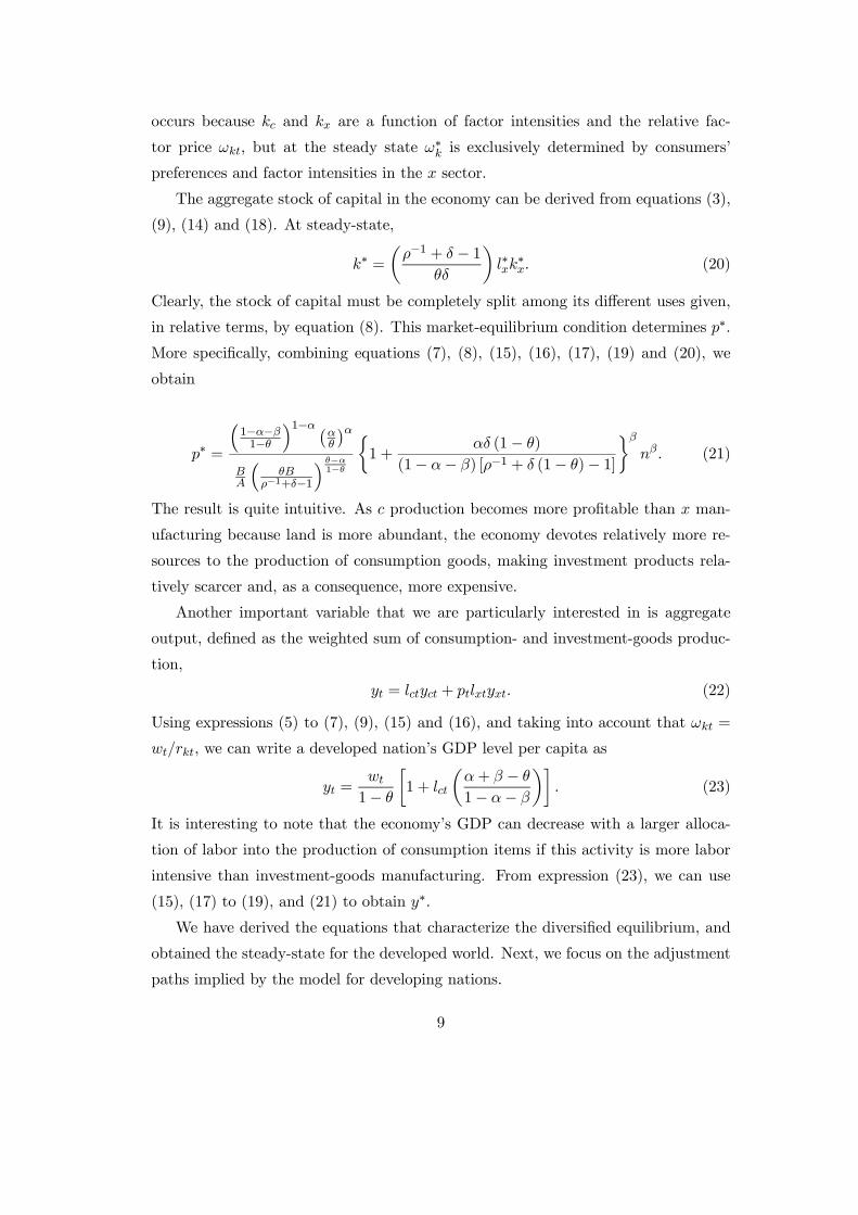
convergence drives the whole convergence process. Figure 3 plots average growth rates
for economies that start the convergence process with different initial relative income
levels and land/labor ratios for that case. The average growth rate is computed
over a 26-period interval. Since the model was calibrated with annual data, this time
interval is the one used, for example, by MRW, and Nonneman and Vanhoudt (1996).
In Figure 3, we see that the time series of growth rates is driven by diminishing
returns to capital accumulation. That is, when we fix the n, average growth rates
decrease as the economy gets closer to its steady state. In the cross section, however,
economies that start closer to the balanced-growth path can show larger average
growth rates. For example, the growth rate when n = 0.2 and initial income is 0.55
is larger than the growth rates shown by any n ≥ 0.81 with initial income bigger orequal than 0.45. If we have a sufficiently large sample, this does not seem to be a
problem, because the average across different land-labor ratios is clearly downward
sloping and driven by diminishing returns. But if we use a relatively small sample,
we may not find a negative relationship between initial income and posterior growth.
For example, suppose that our small sample is composed by the economies depicted
in the chart that deliver average growth rates between 1.05 and 1.50 percent. If we
ran a linear regression of growth rates on initial income, the estimated coefficient
21
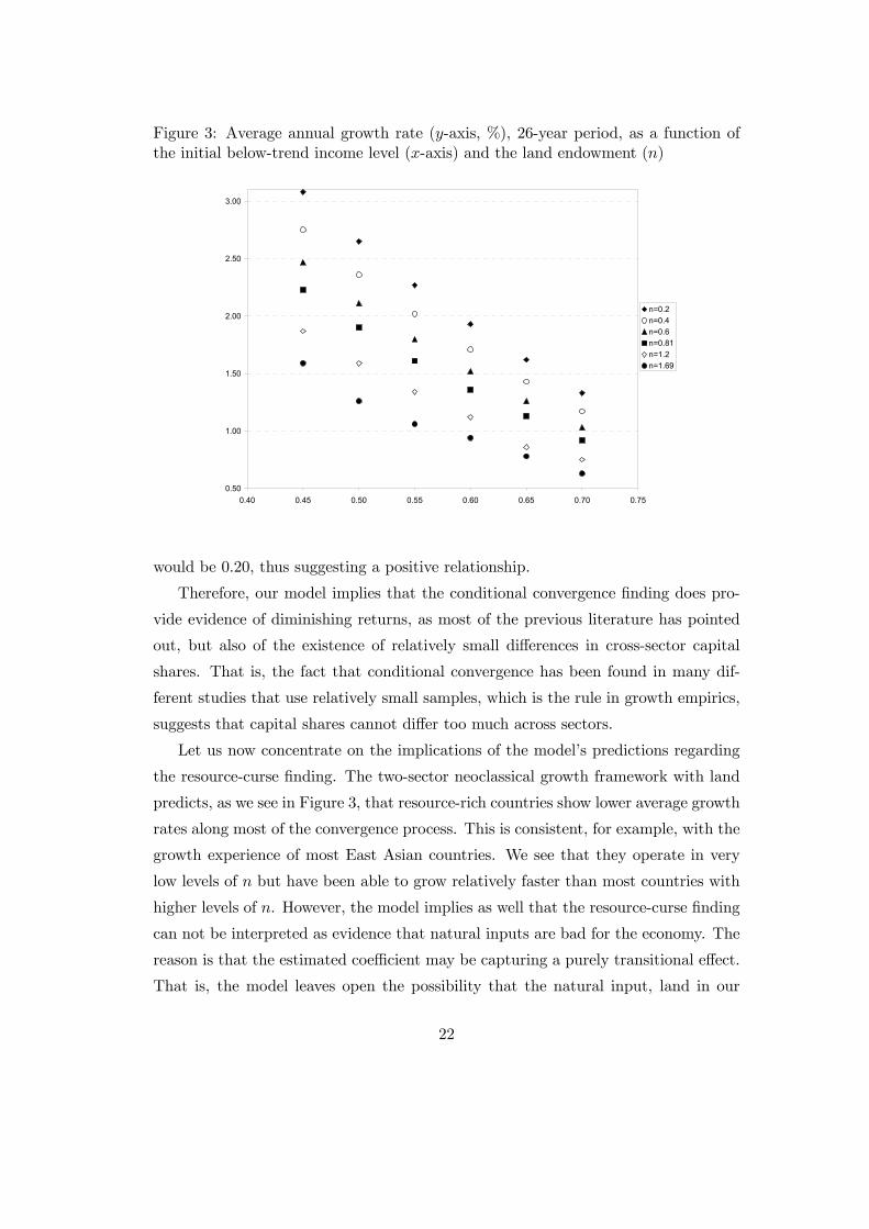
Figure 3: Average annual growth rate (y-axis, %), 26-year period, as a function ofthe initial below-trend income level (x-axis) and the land endowment (n)
0.50
1.00
1.50
2.00
2.50
3.00
0.40 0.45 0.50 0.55 0.60 0.65 0.70 0.75
n=0.2n=0.4n=0.6n=0.81n=1.2n=1.69
would be 0.20, thus suggesting a positive relationship.
Therefore, our model implies that the conditional convergence finding does pro-
vide evidence of diminishing returns, as most of the previous literature has pointed
out, but also of the existence of relatively small differences in cross-sector capital
shares. That is, the fact that conditional convergence has been found in many dif-
ferent studies that use relatively small samples, which is the rule in growth empirics,
suggests that capital shares cannot differ too much across sectors.
Let us now concentrate on the implications of the model’s predictions regarding
the resource-curse finding. The two-sector neoclassical growth framework with land
predicts, as we see in Figure 3, that resource-rich countries show lower average growth
rates along most of the convergence process. This is consistent, for example, with the
growth experience of most East Asian countries. We see that they operate in very
low levels of n but have been able to grow relatively faster than most countries with
higher levels of n. However, the model implies as well that the resource-curse finding
can not be interpreted as evidence that natural inputs are bad for the economy. The
reason is that the estimated coefficient may be capturing a purely transitional effect.
That is, the model leaves open the possibility that the natural input, land in our
22
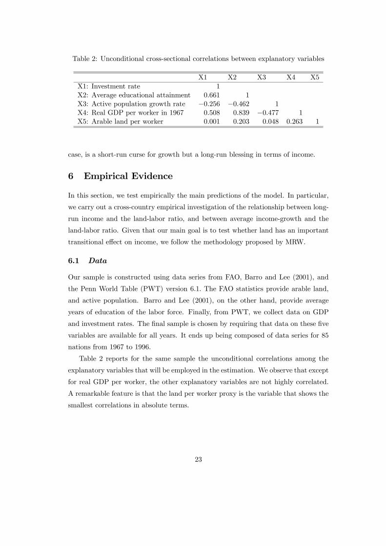
Table 2: Unconditional cross-sectional correlations between explanatory variables
X1 X2 X3 X4 X5X1: Investment rate 1X2: Average educational attainment 0.661 1X3: Active population growth rate −0.256 −0.462 1X4: Real GDP per worker in 1967 0.508 0.839 −0.477 1X5: Arable land per worker 0.001 0.203 0.048 0.263 1
case, is a short-run curse for growth but a long-run blessing in terms of income.
6 Empirical Evidence
In this section, we test empirically the main predictions of the model. In particular,
we carry out a cross-country empirical investigation of the relationship between long-
run income and the land-labor ratio, and between average income-growth and the
land-labor ratio. Given that our main goal is to test whether land has an important
transitional effect on income, we follow the methodology proposed by MRW.
6.1 Data
Our sample is constructed using data series from FAO, Barro and Lee (2001), and
the Penn World Table (PWT) version 6.1. The FAO statistics provide arable land,
and active population. Barro and Lee (2001), on the other hand, provide average
years of education of the labor force. Finally, from PWT, we collect data on GDP
and investment rates. The final sample is chosen by requiring that data on these five
variables are available for all years. It ends up being composed of data series for 85
nations from 1967 to 1996.
Table 2 reports for the same sample the unconditional correlations among the
explanatory variables that will be employed in the estimation. We observe that except
for real GDP per worker, the other explanatory variables are not highly correlated.
A remarkable feature is that the land per worker proxy is the variable that shows the
smallest correlations in absolute terms.
23
6.2 Empirical specification and results
In line with MRW, we consider the following unrestricted empirical specification to
explain long-run income levels:
ln yi1996 = α0 + α1 ln ski + α2 ln shi + α3 ln (GPOPi + g + δ) + α4 lnni;
where ski, shi, GPOPi, and ni are, respectively, the investment rate, the average
educational attainment, the active population growth rate, and the land-labor ratio
for country i, and are calculated as the mean value for the period 1967 to 1996; the
other variable, yi1996, represents the level of real GDP per worker in country i in
1996. From the last expression, we derive the following steady-state output growth
regression:
ln yi1996−ln yi1967 = α0+α1 ln ski+α2 ln shi+α3 ln (GPOPi + g + δ)+α4 lnni−ln yi1967.
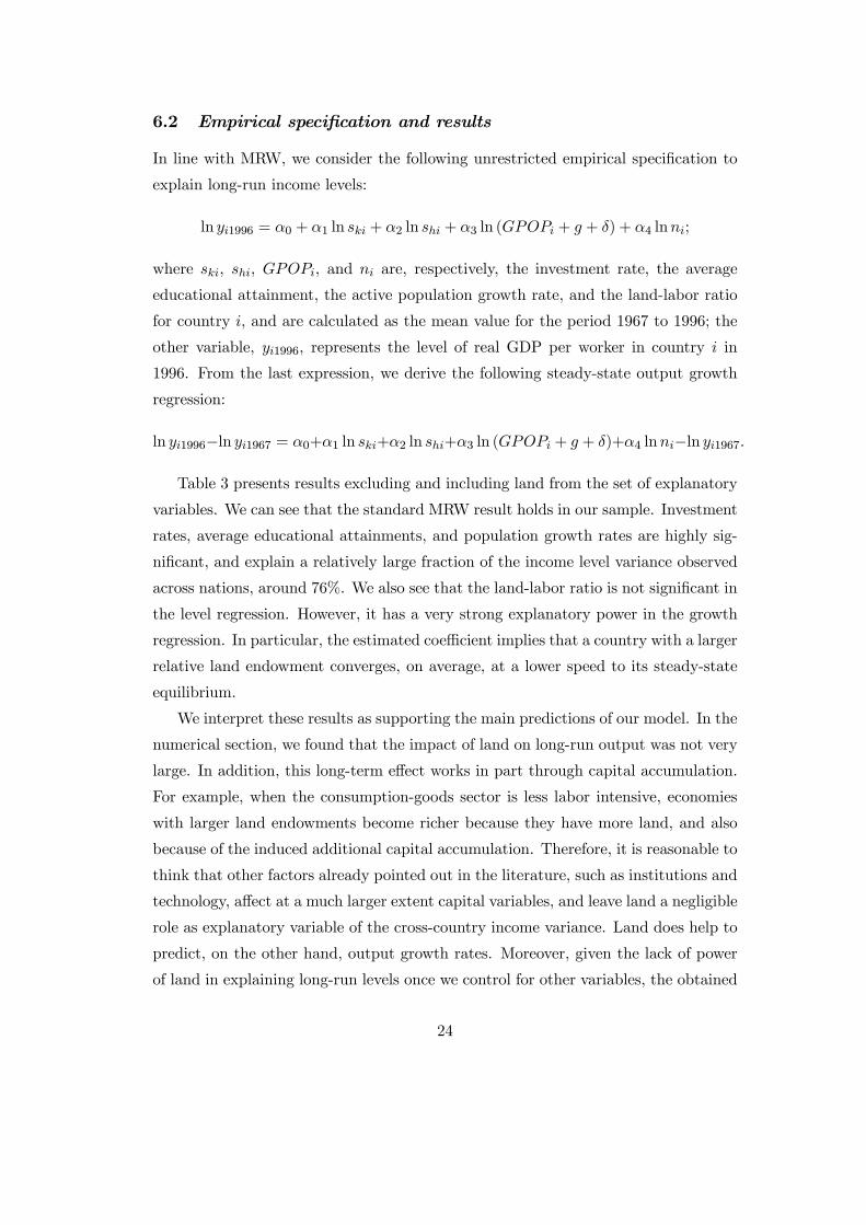
Table 3 presents results excluding and including land from the set of explanatory
variables. We can see that the standard MRW result holds in our sample. Investment
rates, average educational attainments, and population growth rates are highly sig-
nificant, and explain a relatively large fraction of the income level variance observed
across nations, around 76%. We also see that the land-labor ratio is not significant in
the level regression. However, it has a very strong explanatory power in the growth
regression. In particular, the estimated coefficient implies that a country with a larger
relative land endowment converges, on average, at a lower speed to its steady-state
equilibrium.
We interpret these results as supporting the main predictions of our model. In the
numerical section, we found that the impact of land on long-run output was not very
large. In addition, this long-term effect works in part through capital accumulation.
For example, when the consumption-goods sector is less labor intensive, economies
with larger land endowments become richer because they have more land, and also
because of the induced additional capital accumulation. Therefore, it is reasonable to
think that other factors already pointed out in the literature, such as institutions and
technology, affect at a much larger extent capital variables, and leave land a negligible
role as explanatory variable of the cross-country income variance. Land does help to
predict, on the other hand, output growth rates. Moreover, given the lack of power
of land in explaining long-run levels once we control for other variables, the obtained
24
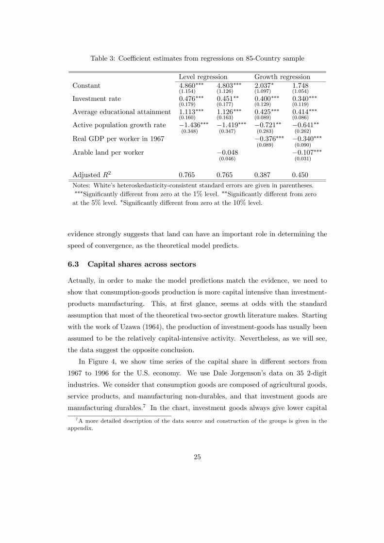
Table 3: Coefficient estimates from regressions on 85-Country sample
Level regression Growth regressionConstant 4.860
(1.154)
∗∗∗ 4.803(1.126)
∗∗∗ 2.037(1.097)
∗ 1.748(1.054)
Investment rate 0.476(0.179)
∗∗∗ 0.451(0.177)
∗∗ 0.400(0.129)
∗∗∗ 0.340(0.119)
∗∗∗
Average educational attainment 1.113(0.160)
∗∗∗ 1.126(0.163)
∗∗∗ 0.425(0.089)
∗∗∗ 0.414(0.086)
∗∗∗
Active population growth rate −1.436(0.348)
∗∗∗ −1.419(0.347)
∗∗∗ −0.721(0.283)
∗∗ −0.641(0.262)
∗∗
Real GDP per worker in 1967 −0.376(0.089)
∗∗∗ −0.340(0.090)
∗∗∗
Arable land per worker −0.048(0.046)
−0.107(0.031)
∗∗∗
Adjusted R2 0.765 0.765 0.387 0.450
Notes: White’s heteroskedasticity-consistent standard errors are given in parentheses.∗∗∗Significantly different from zero at the 1% level. ∗∗Significantly different from zeroat the 5% level. ∗Significantly different from zero at the 10% level.
evidence strongly suggests that land can have an important role in determining the
speed of convergence, as the theoretical model predicts.
6.3 Capital shares across sectors
Actually, in order to make the model predictions match the evidence, we need to
show that consumption-goods production is more capital intensive than investment-
products manufacturing. This, at first glance, seems at odds with the standard
assumption that most of the theoretical two-sector growth literature makes. Starting
with the work of Uzawa (1964), the production of investment-goods has usually been
assumed to be the relatively capital-intensive activity. Nevertheless, as we will see,
the data suggest the opposite conclusion.
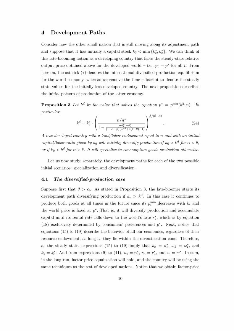
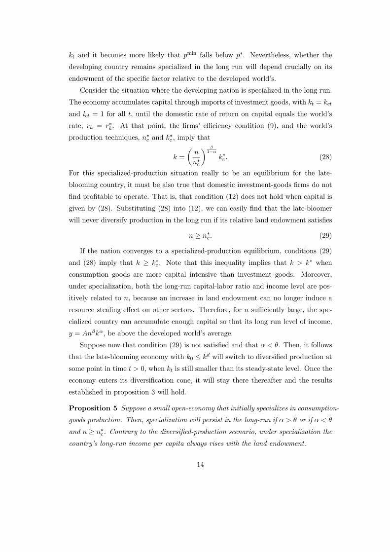
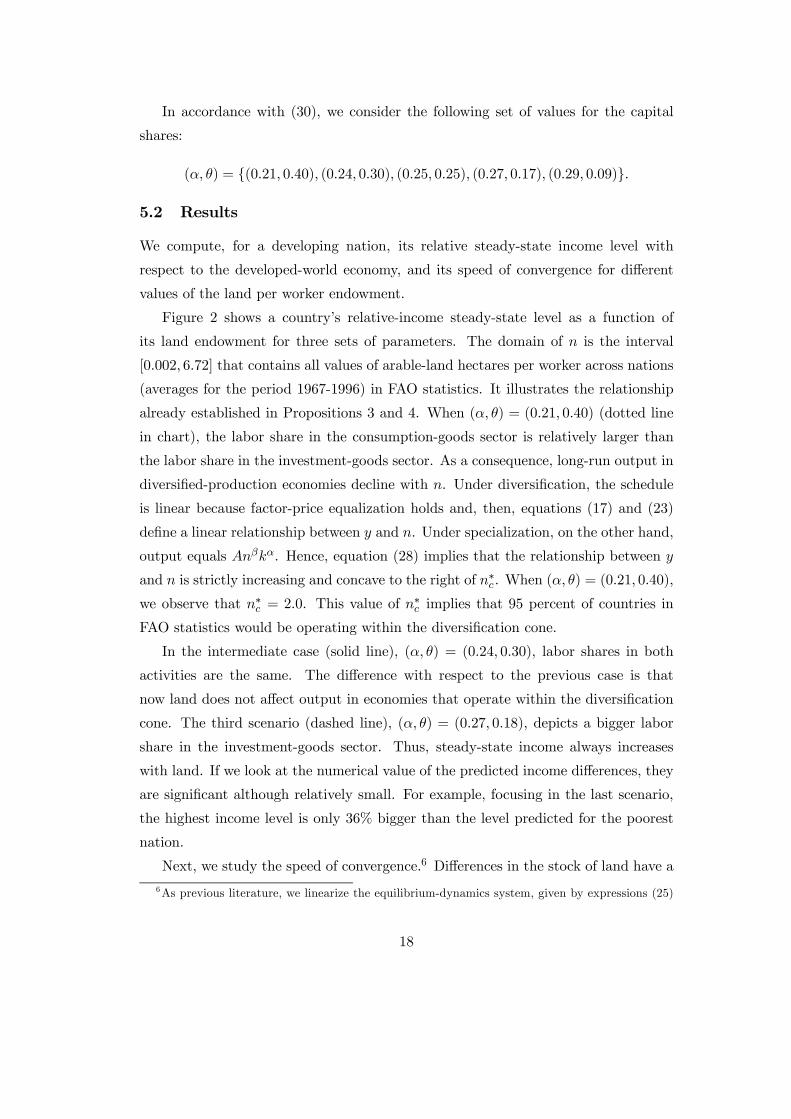
In Figure 4, we show time series of the capital share in different sectors from
1967 to 1996 for the U.S. economy. We use Dale Jorgenson’s data on 35 2-digit
industries. We consider that consumption goods are composed of agricultural goods,
service products, and manufacturing non-durables, and that investment goods are
manufacturing durables.7 In the chart, investment goods always give lower capital
7A more detailed description of the data source and construction of the groups is given in theappendix.
25
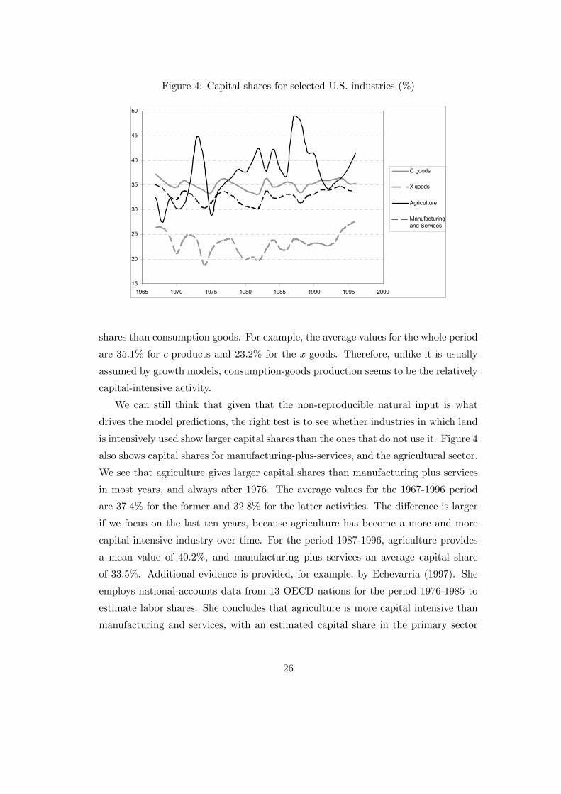
Figure 4: Capital shares for selected U.S. industries (%)
15
20
25
30
35
40
45
50
1965 1970 1975 1980 1985 1990 1995 2000
C goods
X goods
Agriculture
Manufacturingand Services
shares than consumption goods. For example, the average values for the whole period
are 35.1% for c-products and 23.2% for the x-goods. Therefore, unlike it is usually
assumed by growth models, consumption-goods production seems to be the relatively
capital-intensive activity.
We can still think that given that the non-reproducible natural input is what
drives the model predictions, the right test is to see whether industries in which land
is intensively used show larger capital shares than the ones that do not use it. Figure 4
also shows capital shares for manufacturing-plus-services, and the agricultural sector.
We see that agriculture gives larger capital shares than manufacturing plus services
in most years, and always after 1976. The average values for the 1967-1996 period
are 37.4% for the former and 32.8% for the latter activities. The difference is larger
if we focus on the last ten years, because agriculture has become a more and more
capital intensive industry over time. For the period 1987-1996, agriculture provides
a mean value of 40.2%, and manufacturing plus services an average capital share
of 33.5%. Additional evidence is provided, for example, by Echevarria (1997). She
employs national-accounts data from 13 OECD nations for the period 1976-1985 to
estimate labor shares. She concludes that agriculture is more capital intensive than
manufacturing and services, with an estimated capital share in the primary sector
26
more than 20 percentage-points larger than in the other two.
Still, we could consider that there is a caveat with the previous exercise. The rea-
son is that the share of land does not appear separately in the national accounts; it
is actually included in either capital or labor, and there is no easy method to remove
it. There is evidence that even controlling for the land share, the capital elasticity
in agriculture is large. For example, Echevarria (2000) finds a capital share of 43%
in agriculture for the Canadian economy once the value of land is excluded. Early
cross-country studies focusing on the agricultural sector, however, such as Hayami
and Ruttan (1985), seem to find smaller capital shares after controlling for the con-
tribution of land. These studies estimate an average capital share of structures and
equipment of around 10 percent. Which has led to the growth literature concerned
with cross-country income disparities to assume that agriculture is less capital inten-
sive than manufacturing.8 This conclusion is not correct when we take into account
that capital in agriculture is composed not only of structures and equipment but also
of livestock and orchards, as Mundlak et al. (2000), among others, point out. Taken
both components together, and controlling for the contribution of land, the estimated
elasticity of capital in agricultural output by the early studies is between 33% and
47%. In addition, Mundlak et al. (1999) that surveys this early literature criticizes
it for not correcting for potential temporal and cross-country fixed-effect problems.
These authors employ a balanced data panel of 37 developed and developing coun-
tries for a 21-year period, 1970-1990. Using appropriate techniques for panel data
estimation, they conclude that, after controlling for land, the agricultural sector is
more capital intensive than the non-primary activities, with a capital share above
40%.
Taken together, the evidence suggests that consumption-goods production is a
more capital intensive activity than investment-goods production. Moreover, most
studies show that primary-products have also larger capital elasticities than non-
primary industries. Therefore, the usual assumption made by a big part of the
growth literature that consumption-goods production and agriculture are less capital
intensive is not well founded. Most of the evidence points to the opposite direction. As
a consequence, the predictions of the model are consistent with most of the evidence.
8See, for example, Gollin, Parente and Rogerson (2002), and Caselli and Coleman (2001).
27
7 Conclusion
This paper has studied an open-economy version of the two-sector neoclassical growth
model with land. In sharp contrast to the predictions of the standard neoclassical
growth framework, in the two-sector model with land two economies that are at
the same distance of their steady states do not converge at the same speed if they
have different land endowments. Moreover, an economy that is closer to its long-run
equilibrium can show larger growth rates. The reason is that our model predicts
that land, besides having long-run effects, has also transitional growth effects. More
specifically, even though the share of land in GDP is only around 5 percent, calibration
has shown that its transitional effects on output growth can be substantial, and more
important than its direct impact on long-run income. This is the case when capital
shares differ across sectors.
We have argued that these results offer an alternative interpretation of the condi-
tional convergence and resource curse findings. The model suggests that the former
finding does provide evidence of diminishing returns, as most of the previous litera-
ture has pointed out, but also of relatively small cross-sector capital-share differences.
Regarding the latter finding, the model predicts that the lower growth rates shown
by resource-richer economies does not lead to the conclusion that natural riches are
a long-run curse. The reason is that the resource curse evidence may be capturing a
purely transitional phenomenon due to the effect of natural riches (land in our model)
on the speed of convergence.
The predictions of our setup regarding long-run income levels of developing na-
tions are also in sharp contrast to the ones of more standard open-economy two-sector
neoclassical growth models that only include mobile factors. First, nations that start
their development paths at the same date may converge to different income levels.
This occurs if they have distinct land endowments. Second, identical nations that
differ only in their timing of development converge to the same long-run income level.
Finally, long-run specialization does not necessarily imply a level of per capita in-
come lower than the world’s average. The key to this results is the uniqueness of the
aggregate capital-labor ratio compatible with a given return to capital in the model
with land.
Finally, the paper has presented empirical evidence that tests the predictions of
the model. Unlike previous studies, we have focused on the effect of land on growth
28
and income levels. Regression results suggest that land has a negative impact in
transitional growth, with no statistically-significant independent-effect on long-run
income levels. This finding does not mean that land has no effect in long-run income.
It suggests that its effect works primarily through other variables such as capital
investment and institutions already pointed out by the literature. We have also
provided data that supports that capital shares are larger in land-intensive sectors.
This last piece of evidence should lead the growth literature to revise the widely-
used assumption that consumption-goods and agriculture are less capital intensive
activities than investment-goods and manufacturing, respectively. In sum, we have
argued that the empirical evidence is consistent with the model predictions.
29
A Proofs
Proof of proposition 1. Suppose that the agricultural technology is not used. Afirm that has access to this technology will like to open if it makes profits for theprices (say rk, wt, rn and p) that prevail in the equilibrium where the economy islocated. In particular, given N > 0, this firm choosesKat and Lat to maximize profitsΠat, which is equivalent to maximizing
A
µKat
N
¶αµLat
N
¶1−α−β− rkt
Kat
N− wt
Lat
N− rnt. (32)
The maximum level of profits, per unit of land, then equals
ΠatN
= βA1β
µ1− α− β
wt
¶1−α−ββ
µαkrkt
¶αβ
− rnt. (33)
In an equilibrium in which this type of firm does not operate, it must be true thatrnt = 0. Hence, in expression (33) maximum profits are strictly positive, for all wt
and rkt, and domestic firms will always supply agricultural products.
Proof of proposition 2. Manufacturers’ profits equal
Πxt = ptBKθmtL
1−θmt − rktKmt −wtLmt. (34)
At the maximum, it must hold that
max0≤Kmt≤Kt0≤Lmt≤L
Πmt = Kmt
"rkt
µ1− θ
θ
¶−wt
µrktθptB
¶ 11−θ#. (35)
Manufacturing firms will want to enter the market if and only if they make profits,that is, if and only if
ptB >³rkθ
´θ µ wt
1− θ
¶1−θ, (36)
>From optimality conditions (9) and (11) for agricultural-goods producers, we obtainexpression (12) for rk = rk, wt = wt and pt = pt.
Proof of proposition 3. The value kd comes from its definition, and equations(12), (15), (16), (19) and(21). In addition, we know that the developing country willinitially specialize in consumption goods if and only if p∗ < pmin (k0;n), and thatpmin (k;n) decreases with k if θ > α, and it increases with k if θ < α.
Proof of proposition 4. It directly follows from the text except for the pattern ofproduction when α > θ. In that case, the economy will remain diversified in the longrun as long as kd ≥ k∗x. Taking into account (15), (16) and (24) this condition holds
whenever n/n∗ ≤³
α(1−θ)θ(1−α−β)
´α−θβ³1 + αδ(1−θ)
(1−α−β)(ρ−1+δ(1−θ)−1)´, where both terms in
brackets are greater than one.
30
Proof of proposition 5. It directly follows from the text.
Proof of proposition 6. It directly follows from the text.
B Data Appendix
• Income (GDP), and investment rates [Source: PWT 6.1]
Cross-country real GDP per capita (dollars, chain index), real investment shares, andpopulation size (thousands of people) are taken from the Penn World Tables, Ver-sion 6.1 (PWT 6.1), on-line at http://datacentre2.chass.utoronto.ca/pwt/. Incomeseries are expressed in 1996 international prices.
• Labor force, and arable land [Source: FAO]
The cross-country data set on active population (thousands of workers) and arableland (thousands of hectares) comes from the Food and Agriculture Organization ofthe United Nations Statistics, FAOSTAT. Worker for the active population variableis usually a census definition based on economically active population. Arable landper worker is measured in hectares.
• Education [Source: Barro and Lee (2001)]
Annual data on educational attainment are the sum of the average number of yearsof primary, secondary and tertiary education in labor force for the population groupover age 15.
• Capital shares [Source: Dale Jorgenson]
Annual data on the value of capital inputs and the value of labor inputs per sector areobtained form Dale Jorgenson’s web site, http://post.economics.harvard.edu/faculty/jorgenson/data/35klem.html. The database is described, for example, in Jorgensonand Stiroh (2000). It covers 35 sectors at the 2-digit SIC level for the U.S. economy.
We group sectors as follows. Services includes: transportation; communications;electric utilities; gas utilities; trade; finance insurance and real estate; and other ser-vices. Manufacturing durables includes: lumber and wood; furniture and fixtures;stone, clay, glass; primary metal; fabricated metal; machinery, non-electrical; electri-cal machinery; motor vehicles; transportation equipment & ordnance; instruments;and misc. manufacturing. Manufacturing non-duranbles is composed of the sectors:food and kindred products; tobacco; textile mill products; apparel; paper and allied;printing, publishing and allied; chemicals; petroleum and coal products; rubber andmisc. plastics; and leather.
31
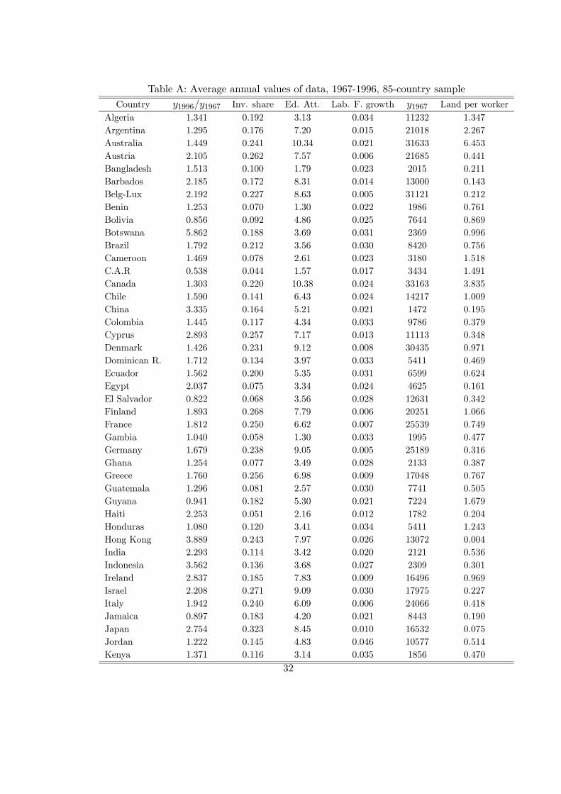
Table A: Average annual values of data, 1967-1996, 85-country sample
Country y1996/y1967 Inv. share Ed. Att. Lab. F. growth y1967 Land per workerAlgeria 1.341 0.192 3.13 0.034 11232 1.347Argentina 1.295 0.176 7.20 0.015 21018 2.267Australia 1.449 0.241 10.34 0.021 31633 6.453Austria 2.105 0.262 7.57 0.006 21685 0.441Bangladesh 1.513 0.100 1.79 0.023 2015 0.211Barbados 2.185 0.172 8.31 0.014 13000 0.143Belg-Lux 2.192 0.227 8.63 0.005 31121 0.212Benin 1.253 0.070 1.30 0.022 1986 0.761Bolivia 0.856 0.092 4.86 0.025 7644 0.869Botswana 5.862 0.188 3.69 0.031 2369 0.996Brazil 1.792 0.212 3.56 0.030 8420 0.756Cameroon 1.469 0.078 2.61 0.023 3180 1.518C.A.R 0.538 0.044 1.57 0.017 3434 1.491Canada 1.303 0.220 10.38 0.024 33163 3.835Chile 1.590 0.141 6.43 0.024 14217 1.009China 3.335 0.164 5.21 0.021 1472 0.195Colombia 1.445 0.117 4.34 0.033 9786 0.379Cyprus 2.893 0.257 7.17 0.013 11113 0.348Denmark 1.426 0.231 9.12 0.008 30435 0.971Dominican R. 1.712 0.134 3.97 0.033 5411 0.469Ecuador 1.562 0.200 5.35 0.031 6599 0.624Egypt 2.037 0.075 3.34 0.024 4625 0.161El Salvador 0.822 0.068 3.56 0.028 12631 0.342Finland 1.893 0.268 7.79 0.006 20251 1.066France 1.812 0.250 6.62 0.007 25539 0.749Gambia 1.040 0.058 1.30 0.033 1995 0.477Germany 1.679 0.238 9.05 0.005 25189 0.316Ghana 1.254 0.077 3.49 0.028 2133 0.387Greece 1.760 0.256 6.98 0.009 17048 0.767Guatemala 1.296 0.081 2.57 0.030 7741 0.505Guyana 0.941 0.182 5.30 0.021 7224 1.679Haiti 2.253 0.051 2.16 0.012 1782 0.204Honduras 1.080 0.120 3.41 0.034 5411 1.243Hong Kong 3.889 0.243 7.97 0.026 13072 0.004India 2.293 0.114 3.42 0.020 2121 0.536Indonesia 3.562 0.136 3.68 0.027 2309 0.301Ireland 2.837 0.185 7.83 0.009 16496 0.969Israel 2.208 0.271 9.09 0.030 17975 0.227Italy 1.942 0.240 6.09 0.006 24066 0.418Jamaica 0.897 0.183 4.20 0.021 8443 0.190Japan 2.754 0.323 8.45 0.010 16532 0.075Jordan 1.222 0.145 4.83 0.046 10577 0.514Kenya 1.371 0.116 3.14 0.035 1856 0.470
32
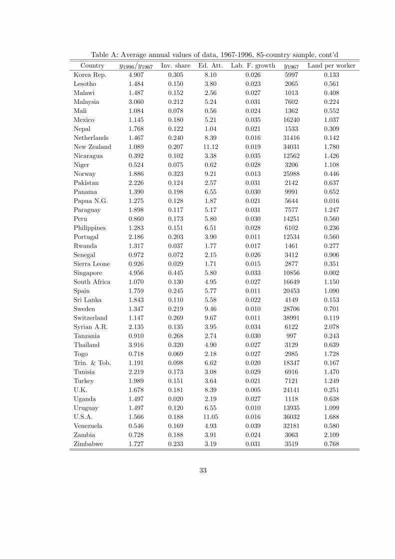
Table A: Average annual values of data, 1967-1996, 85-country sample, cont’d
Country y1996/y1967 Inv. share Ed. Att. Lab. F. growth y1967 Land per workerKorea Rep. 4.907 0.305 8.10 0.026 5997 0.133Lesotho 1.484 0.150 3.80 0.023 2065 0.561Malawi 1.487 0.152 2.56 0.027 1013 0.408Malaysia 3.060 0.212 5.24 0.031 7602 0.224Mali 1.084 0.078 0.56 0.024 1362 0.552Mexico 1.145 0.180 5.21 0.035 16240 1.037Nepal 1.768 0.122 1.04 0.021 1533 0.309Netherlands 1.467 0.240 8.39 0.016 31416 0.142New Zealand 1.089 0.207 11.12 0.019 34031 1.780Nicaragua 0.392 0.102 3.38 0.035 12562 1.426Niger 0.524 0.075 0.62 0.028 3206 1.108Norway 1.886 0.323 9.21 0.013 25988 0.446Pakistan 2.226 0.124 2.57 0.031 2142 0.637Panama 1.390 0.198 6.55 0.030 9991 0.652Papua N.G. 1.275 0.128 1.87 0.021 5644 0.016Paraguay 1.898 0.117 5.17 0.031 7577 1.247Peru 0.860 0.173 5.80 0.030 14251 0.560Philippines 1.283 0.151 6.51 0.028 6102 0.236Portugal 2.186 0.203 3.90 0.011 12534 0.560Rwanda 1.317 0.037 1.77 0.017 1461 0.277Senegal 0.972 0.072 2.15 0.026 3412 0.906Sierra Leone 0.926 0.029 1.71 0.015 2877 0.351Singapore 4.956 0.445 5.80 0.033 10856 0.002South Africa 1.070 0.130 4.95 0.027 16649 1.150Spain 1.759 0.245 5.77 0.011 20453 1.090Sri Lanka 1.843 0.110 5.58 0.022 4149 0.153Sweden 1.347 0.219 9.46 0.010 28706 0.701Switzerland 1.147 0.269 9.67 0.011 38991 0.119Syrian A.R. 2.135 0.135 3.95 0.034 6122 2.078Tanzania 0.910 0.268 2.74 0.030 997 0.243Thailand 3.916 0.320 4.90 0.027 3129 0.639Togo 0.718 0.069 2.18 0.027 2985 1.728Trin. & Tob. 1.191 0.098 6.62 0.020 18347 0.167Tunisia 2.219 0.173 3.08 0.029 6916 1.470Turkey 1.989 0.151 3.64 0.021 7121 1.249U.K. 1.678 0.181 8.39 0.005 24141 0.251Uganda 1.497 0.020 2.19 0.027 1118 0.638Uruguay 1.497 0.120 6.55 0.010 13935 1.099U.S.A. 1.566 0.188 11.05 0.016 36032 1.688Venezuela 0.546 0.169 4.93 0.039 32181 0.580Zambia 0.728 0.188 3.91 0.024 3063 2.109Zimbabwe 1.727 0.233 3.19 0.031 3519 0.768
33
ReferencesAtkeson, A., and P. Kehoe, “Paths of development for early- and late-bloomers
in a Dynamic Heckscher-Ohlin Model,” Federal Reserve Bank of Minneapolisworking paper, 2000.
Barro, R.J., “Economic Growth in a Cross Section of Countries,” Quarterly Journalof Economics 106:407-443, 1991.
Barro, R.J., and J.W. Lee, “International Data on Educational Attainment: Up-dates and Implications,” Oxford Economic Papers 53:541-563, July 2001.
Barro, R.J. and Sala-i-Martin, X., Economic Growth, Macmillan, New York, NY,1995.
Caselli, F., and W.J. Coleman, “The U.S. Structural Transformation and RegionalConvergence: A Reinterpretation” Journal of Political Economy 109(3):584-616, June 2001.
Caselli, Francesco, Gerardo Esquivel, and Fernando Lefort, “Reopening the Conver-gence Debate: A New Look at Cross—Country Growth Empirics,” Journal ofEconomic Growth 1:363—389, September 1996.
Doppelhofer, D., R. Miller and X. Sala-i-Martin, “Determinants of Long-TermGrowth: A Bayesian Averaging of Classical Estimates (BACE) Approach,”American Economic Review, September 2004.
Eaton, J., and S. Kortum, “Trade in Capital Goods,” European Economic Review45:1195-1235, 2001.
Echevarria, C., “Changes in Sectoral Composition Associated with Economic Growth,”International Economic Review 38(2):431-452, May 1997.
Echevarria, C., “Nonhomothetic Preferences and Growth,” Journal of InternationalTrade and Economic Development, 9(2):151-172, June 2000.
Galor, O., O. Moav and D. Vollrath, “Land Inequality and the Emergence of HumanCapital Promoting Institutions,” mimeo, Brown University, 2005.
Galor, O., and A. Mountford, “Trading Population for Productivity” mimeo, BrownUniversity, 2004.
Gollin, D., S.L. Parente and R. Rogerson, “The Role of Agriculture in Development,”American Economic Review 92(2):160-164, May 2002.
Gollin, D., S.L. Parente and R. Rogerson, “Structural Transformation and Cross-Country Income Differences,” mimeo, Arizona State University, 2002.
Hansen, G.D., and E.C. Prescott, “Malthus to Solow,” American Economic Review,1205-1217, September 2002.
Hayami, Y., and V. Ruttan, Agricultural Development: An International Perspec-tive, Revised and Extended Edition, John Hopkins University Press, 1985.
Jorgenson, D.W., and K.J. Stiroh, “Raising the Speed Limit: U.S. Economic Growthin the Information Age,” Brookings Papers on Economic Activity 1, 125-211,2000
Kögel, T., and A. Prskawetz, “Agricultural Productivity Growth and Escape fromthe Malthusian Trap,” Journal of Economic Growth 6:337-357, 2001.
34
Mankiw, G., Romer, D. and Weil, D., “A Contribution to the Empirics of EconomicGrowth,” Quarterly Journal of Economics, 107:407-437, 1992.
Matsuyama, K., “Agricultural productivity, comparative advantage, and economicgrowth,” Journal of Economic Theory 58:317-334, 1992.
Mountford, A., “Trade, convergence and overtaking,” Journal of International Eco-nomics 46:167-182, 1998.
Mundlak, Y., D.F. Larson and R. Butzer, “Rethinking Within and Between Regres-sions: The Case of Agricultural Production Functions,” Annales d’Economie etde Statistique 55-56: 475-501, 1999.
Mundlak, Y., D.F. Larson and R. Butzer, “A Cross-Country Database for SectorInvestment and Capital,” The World Bank Economic Review 14:371-91, 2000.
Nonneman, W. and Vanhoudt, P., “A Further Augmentation of the Solow Modeland the Empirics of Economic Growth for OECD Countries,” Quarterly Journalof Economics 111:943-953, 1996.
Parente, S.L., and E.C. Prescott, Barriers to Riches, MIT Press, 2000.
Restuccia, D., D.T. Yang and X. Zhu, “Agriculture and Aggregate Productivity: Aquantitative Cross-Country Analysis,” mimeo, University of Toronto, 2004.
Sachs, J.D., and A.M.Warner, “The curse of natural resources,” European EconomicReview 45:827-838, May 2001.
Sala-i-Martin, X., “I Just Ran Two Million Regressions,” American Economic Re-view, Papers and Proceedings, May 1997.
Uzawa, H., “Optimal Growth in a Two-Sector Model of Capital Accumulation,”Review of Economic Studies 34:1-24, January 1964.
Ventura, J., “Growth and Interdependence,” Quarterly Journal of Economics, 57-84,February 1997.
35