DOCUMENTO DE TRABAJO N° 284 UNIVERSIDAD · PDF [email protected]. 1 (1989). In his original paper, Hamilton used an AR(4) speci–cation in or

DEPARTAMENTODE ECONOMÍA

DEPARTAMENTO DE ECONOMÍAPONTIFICIA DEL PERÚUNIVERSIDAD CATÓLICA








DEPARTAMENTO DE ECONOMÍA



DOCUMENTO DE TRABAJO N° 284APPLICATION OF THREE NON-LINEAR ECONOMETRIC APPROACHES TO IDENTIFY BUSINESS CYCLES IN PERU

Gabriel Rodríguez

DOCUMENTO DE ECONOMÍA N° 284

APPLICATION OF THREE NON-LINEAR ECONOMETRIC APPROACHES TO IDENTIFY BUSINESS CYCLES IN PERU Gabriel Rodríguez

Julio, 2010

DEPARTAMENTO DE ECONOMÍA

DOCUMENTO DE TRABAJO 284 http://www.pucp.edu.pe/departamento/economia/images/documentos/DDD284.pdf

http://www.pucp.edu.pe/departamento/economia/images/documentos/DDD284.pdf�

© Departamento de Economía – Pontificia Universidad Católica del Perú, © Gabriel Rodríguez Av. Universitaria 1801, Lima 32 – Perú. Teléfono: (51-1) 626-2000 anexos 4950 - 4951 Fax: (51-1) 626-2874 [email protected] www.pucp.edu.pe/departamento/economia/

Encargada de la Serie: Giovanna Aguilar Andía Departamento de Economía – Pontificia Universidad Católica del Perú, [email protected]

Rodríguez, Gabriel APPLICATION OF THREE NON-LINEAR ECONOMETRIC APPROACHES TO IDENTIFY BUSINESS CYCLES IN PERU / Gabriel Rodríguez Lima, Departamento de Economía, 2010 (Documento de Trabajo 284) Nonlinearities / Asymmetries / STAR Model / Markov-Switching Model / Plucking Model / Recession Times.

Las opiniones y recomendaciones vertidas en estos documentos son responsabilidad de sus autores y no representan necesariamente los puntos de vista del Departamento Economía.

Hecho el Depósito Legal en la Biblioteca Nacional del Perú Nº 2010-06580 ISSN 2079-8466 (Impresa) ISSN 2079-8474 (En línea) Impreso en Cartolan Editora y Comercializadora E.I.R.L. Pasaje Atlántida 113, Lima 1, Perú. Tiraje: 100 ejemplares

mailto:[email protected]�

mailto:[email protected]�

Application of Three Non-Linear EconometricApproaches to Identify Business Cycles in Peru

Gabriel Rodríguez

Ponti�cia Universidad Católica del Perú

Abstract

I use three non-linear econometric models to identify and analyze business cy-cles in the Peruvian economy for the period 1980:1-2008:4. The models arethe Smooth Transition Autoregressive (STAR) model suggested by Teräsvirta(1994), the extended version of the Markov-Switching model proposed by Hamil-ton (1989), and the plucking model of Friedman (1964, 1993). The results indi-cate strong rejection of the null hypothesis of linearity. The majority of modelsidentify quarters concentrated around 1988-1989 and 1990-1991 as recessiontimes. Other important events which happened in the Peruvian economy (nat-ural disaster in 1983, e¤ects of the Asian and Russian crises in 1990s, terroristactivities in 1980s) are not selected except as atypical observations. Most ofmodels also identify the period 1995:1-2008:4 as a very long and stable periodof moderate-high growth rates. From the perspective of the Peruvian economichistory and from a statistical point of view, the MSIAH(3) model is the preferredmodel.

Keywords: Nonlinearities, Asymmetries, STARModel, Markov-Switching Model,Plucking Model, Recession TimesJEL Classi�cation: C22, C52, E32.

Resumen

En este documento se usan tres modelos no lineales econométricos para identi-�car y analizar ciclos económicos en la economía Peruana para el período 1980:1-2008:4. Los modelos son el modelo autoregresivo de transición suave (STAR)propuesto por Terasvirta (1994), la versión extendida del modelo Markov Switch-ing sugerido por Hamilton (1989), y el modelo Plucking de Friedman (1963,1993). Los resultados indican fuerte rechazo de la hipótesis nula de lineali-dad. La mayoría de los modelos identi�can trimestres concentrados alrededorde 1988-1989 y 1990-1991 como recesiones. Otros eventos importantes aconte-cidos en la economía Peruana (desastres naturales en 1983, efectos de las crisisAsiática y Rusa en 1990, actividades terroristas en los años 1980) no son se-leccionadas excepto como observaciones atípicas. La mayoría de los modelostambién identi�can el período 1995:1-2008:4 como un periodo largo y establede tasas de crecimiento moderadas y altas. Desde la perspectiva de la historiaeconómica Peruana y desde un punto de vista estadístico, el modelo MSIAH(3)es el modelo seleccionado.

Palabras Claves: No Linealidades, Asimetrías, Modelo STAR, Modelo MarkovSwitching, Modelo Plucking, RecesionesClassi�cación JEL: C22, C52, E32.

Application of Three Non-Linear EconometricApproaches to Identify Business Cycles in Peru1

Gabriel Rodríguez2

Ponti�cia Universidad Católica del Perú

1 Introduction

Econometric theory suggests that a number of important time-series vari-ables should exhibit non-linear behavior. Two important features of thebusiness cycles literature are the existence of nonlinearities and asymme-tries. For example, Mitchell (1927) and Keynes (1936) noted that businesscontractions are briefer than business expansions, and they are also moresudden and violent. This fact was also found by Neftci (1984) when heanalyzed the behavior of US unemployment rates. Therefore, business �uc-tuations are asymmetric and nonlinear.

There is a large number of nonlinear models; see, for example, Grangerand Teräsvirta (1993) for a survey. A type of model to identify businesscycles is an alternative model that assumes that the transition betweenregimes is caused by an observable variable which belong to the set of in-dependent variables or some other exogenous variable. This model is theSmooth Transition Autoregressive (STAR) model proposed by Teräsvirta(1994). In this model, the transition variable determines the threshold leveland speed (smoothness) parameters driving the transition between bothregimes. The version where the named transition function assumes a logis-tic form appears to be adequate to analyze business cycles. One interestingempirical application is Teräsvirta and Anderson (1992).

Other type of models that assume that the transition between regimesis caused by exogenous but not observable variables (or unknown events) isthe case of the Markov-Switching model, originally proposed by Hamilton

1 I thank useful comments of the Editor and two anonymous referees on an earlierversion of the paper. I am also very grateful to Francisco Nadal de Simone for usefule-mail and phone conversations and for important advise related to the plucking model. Ialso thank comments from participants to the XXIV Meeting of Economists of the CentralReserve Bank of Peru (December 2007). A very preliminary version of this paper appearsas Working Paper 2007-007 of the Central Bank of Peru.

2Address for Correspondence: Gabriel Rodríguez, Department of Economics, Pon-ti�cia Universidad Católica del Perú, Av. Universitaria 1801, Lima 32, Lima,Perú, Telephone: +511-626-2000 (4998), Fax: +511-626-2874. E-Mail Address:[email protected].

1

(1989). In his original paper, Hamilton used an AR(4) speci�cation in or-der to model the growth rate of the US output allowing for only a changein the mean. The results obtained allow to identify phases of recessions invery close concordance with the dates identi�ed by the NBER which usesa large set of leading indicators. After it, the model has been largely usedand extended to include regimen dependence both in variances and autore-gressive parameters. Furthermore, the model has also been extended to themultivariate framework by Krolzig (1997). Some interesting applications areGoodwin (1993) and Bodman and Crosby (2000).

Friedman (1964, 1993) also noted asymmetry in real output behavior inthat amplitude of real output contractions is strongly correlated with thesucceeding expansion, but the amplitude of an expansion is not correlatedwith the amplitude of the succeeding contraction. This observation is thesource of the very known �plucking�model of business cycles. Further ev-idence was found by Delong and Summers (1986), Falk (1986), and Sichel(1993).

Empirical evidence characterized by sudden jumps and slower declinesof the real output gives support to the asymmetries suggested by some non-linear models although in particular in favor of the plucking model. As Kimand Nelson (1999) argue, while these kind of asymmetries are consistent withthe plucking model, they are also consistent with models where recessionsare occasioned by infrequent permanent negative shocks as in the Markov-Switching models. What distinguishes the plucking model is the predictionthat negative shocks are largely transitory, while positive shocks are largelypermanent. Another important characteristic of the plucking model is theexistence of an upper limit to the output, the so named potential output,which is set by the resources available in the economy.

Kim and Nelson (1999) have proposed an econometric speci�cation of theplucking model. The approach o¤ers more possibilities than standard linearmodels such as ARIMA models and the unobserved components modelswhich can not account for asymmetries; see Watson (1986), Clark (1987).

Mills and Wang (2002) have applied the procedure of Kim and Nelson(1999) to the real output time series of the G-7 countries. Interesting per-formance of this approach has also been noted by Galvão (2002), where thismodel is one of the three models capable of reproducing the length of theU.S. business cycles. In this respect, see the special issue about businesscycles published by Empirical Economics in 2002. Some further applica-tions of the plucking model are Rodríguez (2005) and Nadal De Simone andClarke (2007).

The number of empirical studies of business cycles applied to Latin

2

American countries is very scarce. One interesting exception is Mejía-Reyes(2004) where synchronization of business cycles in seven Latin Americancountries is analyzed using classical business cycles approach. This approachis also used by Castillo, Montoro and Tuesta (2006) in order to establishsome stylized facts of the Peruvian economy. In this paper, I apply theabove three described alternative non-linear models to the annual growthrates of the real output of Peru for the period 1980:1-2008:4. I considerthat no other similar research has been done for this country. Some relatedwork but more interested in estimations restricted to the output gap areRodríguez (2010a, 2010b).

I consider that Peruvian time series could o¤er an interesting environ-ment to verify theoretical and practical performance of the di¤erent models.In all the sample period, the behavior of the real output has been di¤er-ent. In the �rst half of the sample, growth rates have been very volatileand economy has been very instable in both economic and political terms.It is around 1992 that government started a process of structural reformwith progressive impact in the performance of the economy. Furthermore,Central Bank o¢ cially adopted an in�ation targeting monetary regime in2002. All these changes have had positive consequences on the stability ofthe economy at the internal and external levels.

Some particular events happened in the sample period are worth to bementioned. The �rst event happened in 1983 in the north of Peru wherea serious natural disaster a¤ected the agricultural sector of the economy.The second event is the presence of the terrorist group named Shining Pathwhich started its armed actions in 1980 a¤ecting many regions of the countryand di¤erent sectors of the economy. The third event was the high in�ationepisodes happened in 1988 caused by di¤erent incoherent �scal and monetarypolicies. The di¤erent �scal and monetary programs applied failed to stophigh in�ation ended in a dramatic hyperin�ation in 1990:2. This event wasstopped in 1990:3 with a new government which dropped dramatically themonetary base and relaxed chaotic behavior of public prices.

All our estimations suggest presence and relevance of nonlinearities andsome atypical observations (outliers) in the real output. Evaluation ofsome linear models suggests presence of autocorrelation in the residuals,squared residuals, presence of autoregressive conditional heteroscedasticityand strong dependence of the residuals. Nonlinear estimation appears to beneeded.

The majority of estimates of the non-linear models identify quarters con-centrated in 1988 and 1990 as recession times. Some events as the naturaldisasters happened in 1983 are only captured as atypical observations but

3

they do not qualify as recession times. Furthermore, the Asian and Russian�nancial crises are not identi�ed as recession times. It means that theseevents probably a¤ected the �nancial sector of the economy but not the realoutput of the economy. Another potential explanation is that they a¤ectedreal sector of the economy but negative growth rates are smaller comparedwith the levels identi�ed by the models. The alternative hypothesis thatarmed and destructive actions of the terrorist group Shining Path couldcause recession periods is di¢ cult to accept according to the estimates. Ac-cording to them, the destruction caused by this terrorist group does notcause recession times in the sense of recurrent negative growth rates.

Another similarity between models is that since 1994-1995, the economyappears to enter in a period of relative sustainable growth. It is supported bythe various structural reforms of the economy in the labor market, �nancialsector, external sector, and adoption of the targeting in�ation system. Allthese measures contributed to the adequate behavior of the economy withless volatility in the evolution of the major macroeconomic variables. There-fore all nonlinear models indicate long duration of the times with moderate-high growth rates.

From the point of view of the statistical evaluation of the di¤erent non-linear models, the MSIAH(3) model shows superior performance. Accordingto the notation of the Section 2.2, it is a Markov-Switching model withintercept, autoregressive parameters and variance dependent of the regimes.In this case, the selected number of regimes is three. This model selectsthe recession times and normal times which are more consistent with visualinspection and with the real events happened in the Peruvian economy. Atthe moment of the testing evaluation, the model performs better than theother selected Markov-Switching models and the other competitive models.

The rest of the paper is organized in the following manner. Section2 brie�y describes the three alternative non-linear methods to be used inthe estimations. Section 3 presents and discusses the results. Section 4concludes.

2 Methodologies

In this section, the three non-linear econometric approaches used in the em-pirical section are brie�y described. In all cases, yt denotes the logarithm ofthe real output at period t and �4yt denotes the annual growth rates of realoutput (yt � yt�4). The �rst model is the Smooth Transition Autoregres-sive (STAR) model proposed by Teräsvirta (1994). The second model is an

4

extended version of the Markov-Switching Autoregressive (MS-AR) modeloriginally suggested by Hamilton (1989). Finally, last model is the pluck-ing model, theoretically proposed by Friedman (1964, 1993) and empiricallyimplemented by Kim and Nelson (1999).

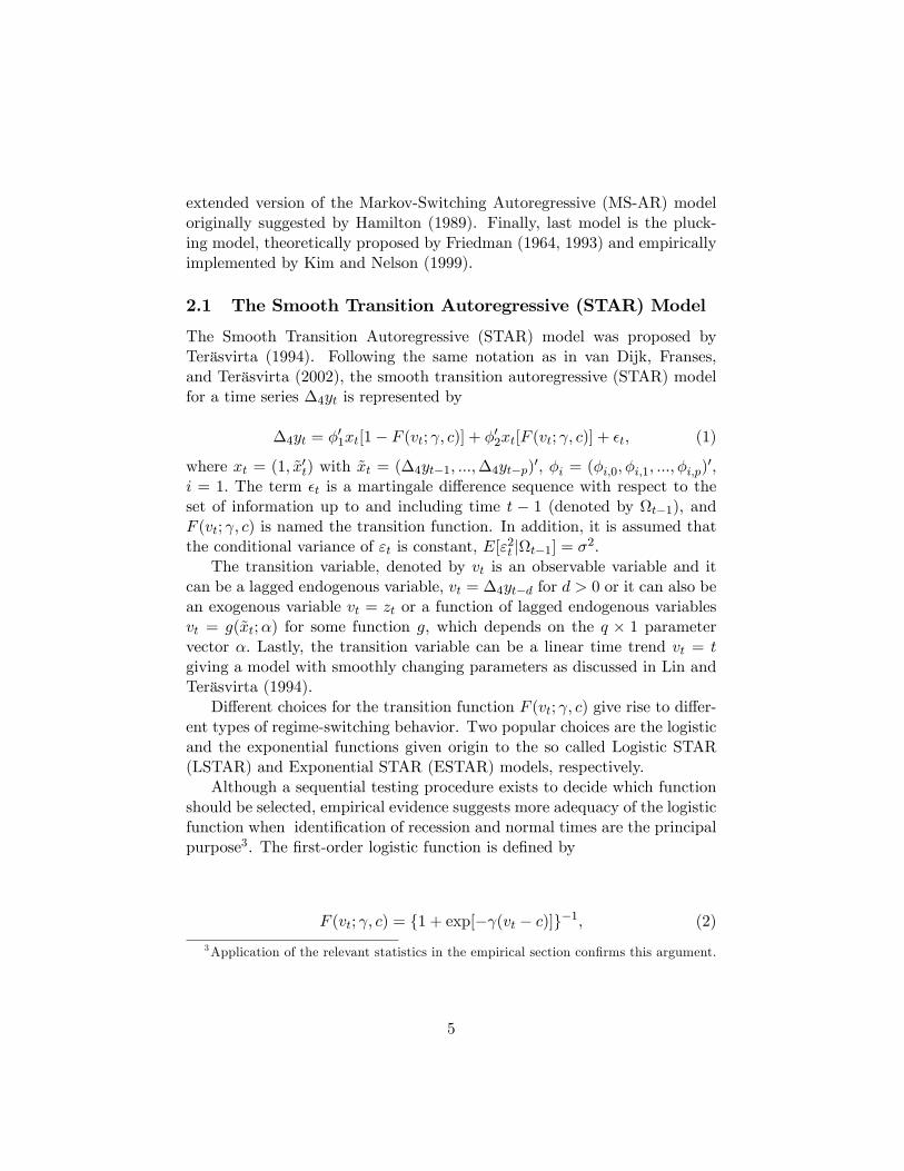
2.1 The Smooth Transition Autoregressive (STAR) Model

The Smooth Transition Autoregressive (STAR) model was proposed byTeräsvirta (1994). Following the same notation as in van Dijk, Franses,and Teräsvirta (2002), the smooth transition autoregressive (STAR) modelfor a time series �4yt is represented by

�4yt = �01xt[1� F (vt; ; c)] + �02xt[F (vt; ; c)] + �t; (1)

where xt = (1; ~x0t) with ~xt = (�4yt�1; :::;�4yt�p)0, �i = (�i;0; �i;1; :::; �i;p)

0,i = 1: The term �t is a martingale di¤erence sequence with respect to theset of information up to and including time t � 1 (denoted by t�1), andF (vt; ; c) is named the transition function. In addition, it is assumed thatthe conditional variance of "t is constant, E["2t jt�1] = �2.

The transition variable, denoted by vt is an observable variable and itcan be a lagged endogenous variable, vt = �4yt�d for d > 0 or it can also bean exogenous variable vt = zt or a function of lagged endogenous variablesvt = g(~xt;�) for some function g, which depends on the q � 1 parametervector �: Lastly, the transition variable can be a linear time trend vt = tgiving a model with smoothly changing parameters as discussed in Lin andTeräsvirta (1994).

Di¤erent choices for the transition function F (vt; ; c) give rise to di¤er-ent types of regime-switching behavior. Two popular choices are the logisticand the exponential functions given origin to the so called Logistic STAR(LSTAR) and Exponential STAR (ESTAR) models, respectively.

Although a sequential testing procedure exists to decide which functionshould be selected, empirical evidence suggests more adequacy of the logisticfunction when identi�cation of recession and normal times are the principalpurpose3. The �rst-order logistic function is de�ned by

F (vt; ; c) = f1 + exp[� (vt � c)]g�1; (2)

3Application of the relevant statistics in the empirical section con�rms this argument.

5

with > 0. In the LSTAR model, the parameter c in (1) or (2) can beinterpreted as the threshold between the two regimes, in the sense that thelogistic function changes monotonically between 0 and 1 as vt increases.The parameter determines the smoothness of the change in the valueof the logistic function and thus, the smoothness of the transition from oneregime to the other. As becomes very large, the logistic function F (vt; ; c)approaches the indicator function I[vt > c], de�ned as I[A] = 1 if A is trueand I[A] = 0 otherwise, and, consequently, the change of F (vt; ; c) from 0to 1 becomes almost instantaneous at vt = c.

Note that the transition function (2) is a special case of the generalnth-order logistic function, de�ned by

F (vt; ; c) = f1 + exp[� nYi=1

(vt � ci)]g�1; (3)

where > 0; c1 6 c2 6 ::: 6 cn: This function can be used to obtain multipleswitches between the two regimes; see for example application of Jansen andTeräsvirta (1996).

In the LSTAR models, the two regimes are associated with small andlarge values of the transition variable vt relative to the parameter c. Thistype of regime-switching can be convenient for modelling, for example, busi-ness cycle asymmetries in distinguishing expansions and recessions. TheLSTAR models has been successfully applied by Teräsvirta and Anderson(1992) and Teräsvirta, Tjøstheim and Granger (1994) to characterize thedi¤erent dynamics of industrial production indexes in a number of OECDcountries.

2.2 The Markov-Switching Model

Let �yt denotes the growth rate of real output in quarter t. The modelof Hamilton (1989) speci�es that �yt follows an autoregressive process oforder 4, that is, an AR(4). Nonlinearity of the model arises because theprocess is subject to discrete shifts in the mean, between high-growth andlow-growth states. These discrete shifts have their own dynamics, speci�edas a two-state �rst-order Markov process. The models is written as

�yt � �st = �1(�yt�1 � �st�1)� :::� �4(�yt�4 � �st�4) + �t; (4)

where �t � i:i:d: N(0; �2): The variable that determines the change of theregime is an unobservable variable denoted by st such that Pr[st = 1jst�1 =1] = p, Pr[st = 0jst�1 = 1] = 1�p, Pr[st = 0jst�1 = 0] = q, Pr[st = 1jst�1 =

6

0] = 1 � q. Therefore, �st = �0 + �1st; and st = 1 if high growth state, 0otherwise.

The model is a non-linear combination of discrete and continuous dynam-ics. An attractive feature of the model is that no prior information regardingthe dates of the two growth periods or the size of the two growth rates isrequired. In particular, note that the low-growth rate need not be negative.Derivation of the sample conditional log-likelihood

PTt=1 ln f [ytjyt�1; yt�2; :::]

is detailed in Hamilton (1989).In notation of Krolzig (1997), the model of Hamilton (1989) is denoted

by MSM(2)-AR(4), that is, a Markov-Switching model with a fourth au-toregressive structure with changing mean between two regimes. However,other speci�cations are available. For example, a model where the mean,the variance and the autoregressive coe¢ cients are regime dependent is de-noted by MSMAH(m)-AR(k) where m indicates the number of states andk re�ects the order of the autoregression. In some cases instead of modelingthe mean as regime dependent parameter, it is considered the intercept asregime dependent. In these cases the notation is MSIAH(m)-AR(k) model.The models where the mean and the intercept are regime dependent o¤erdi¤erent dynamics of adjustment of the variables after a change in regime.

2.3 The Plucking Model

Following the literature of unobserved components (Watson, 1986), it is pos-sible to decompose yt into a trend component and a transitory component,which are denoted as � t and ct, respectively. That is,

yt = � t + ct: (5)

Adopting a similar notation as in Kim and Nelson (1999), I assume thatshocks to the transitory component are a mixture of two di¤erent types ofshocks, which will be denoted �st and ut, respectively. This allows us toaccount for regime shifts or asymmetric deviations of yt from its trend com-ponent. In formal terms, the transitory component and the shocks a¤ectingtheir behavior are speci�ed as follow:

ct = �1ct�1 + �2ct�2 + u�t ; (6)

u�t = �st + ut; (7)

�st = �st; (8)

ut � N(0; �2u;st); (9)

�2u;st = �2u;0(1� st) + �2u;1st; (10)

st = 0; 1; (11)

7

where � 6= 0. In the above speci�cation, the term ut is the usual symmetricshock. The term �st is an asymmetric and discrete shock which is dependentupon an unobserved variable denoted by st which is an indicator variablethat determines the nature of the shocks to the economy (similar as in theMarkov-Switching models previously described). When the economy is nearthe potential or trend output, it can be quali�ed as normal times. In thiscase, st = 0 which implies that �st = 0. In the opposite situation, whichcould be quali�ed as a period of recession, the economy is hit by a transitoryshock potentially with a negative expected value, that is, �st = � < 0. Inthis case, aggregate or other disturbances are plucking the output down.

Note that equations (9) and (10) allow for the possibility that the vari-ance of the symmetric shock ut be di¤erent during normal and recessiontimes. In order to account for a persistence of normal periods or periods ofrecession, it is assumed that st evolves according to a �rst-order Markov-Switching process as in Hamilton (1989). It means that

Pr[st = 1jst�1 = 1] = q;Pr[st = 0jst�1 = 0] = p:

As mentioned by Kim and Nelson (1999), the above speci�cation for thetransitory component of output shares the same idea with the literatureon �stochastic frontier production function�, initially motivated by Aigner,Lowell and Schmidt (1977); see also Goodwin and Sweeney (1993).

The model is completed with the speci�cation of � t, the permanent com-ponent. In this respect, Friedman (1993) suggested that the potential outputcan be approximated by a pure random walk4. In this case, all possible sortsof shocks can produce disturbances on it. In formal terms, this means thatthe permanent component can be speci�ed as follows:

� t = gt�1 + � t�1 + vt; (12)

gt = gt�1 + wt; (13)

vt � N(0; �2v;st); (14)

wt � N(0; �2w); (15)

�2v;st = �2v;0(1� st) + �2v;1st; (16)

where the stochastic trend component � t is subject to two kinds of per-manent shocks: to its level vt and to its growth rate wt. Thus, equations(12)-(15) allow for productivity shocks. Note that it is allowed for the pos-sibility that the variance of the shock to the level may be di¤erent during

4Friedman (1993) named this component �the ceiling maximum feasible output.�

8

normal and recession times. However, variance of the shock to the growthrate is not likely to be systematically di¤erent during the normal and therecession times.

Notice that the model expressed by (5)-(16) nests the model suggestedby Clark (1987). As it is well known, the model of Clark (1987) does notaccount for asymmetries, which in the context of the speci�cation (5)-(16)implies that p = q = 0, � = 0. Furthermore, in the model of Clark (1987),we have �v;0 = �v;1 = �v, and �u;0 = �u;1 = �u:

3 Empirical Results

3.1 Data and Preliminaries

In all next estimations, yt denotes the logarithm of the real output at periodt and �4yt denotes the annual growth rates of real output (yt � yt�4). Thestatistical information is quarterly covering the period 1980:1-2008:4 and itis obtained from the statistics of the Central Bank of Peru.

Figure 1 shows the evolution of the logarithm of the non-seasonal ad-justed real output, and the annual growth rates. One clear evidence of visualinspection of the Figure 1 is the di¤erent behavior of the real output be-fore and after 1990-1991. The �rst period is characterized for high volatilityin growth rates and instability in domestic economy. The second periodis associated with reduced volatility and a more stable economy. In fact,important structural reforms were applied since 1992. Emerging economiesas Peru are characterized for a larger exposition to changes in its economicstructure and consequently there is less stability in its economic cycles. Thestructural reforms were addressed to obtain commercial openness, larger de-velopment of the capital and �nancial markets, more �exibility in the labormarket and a more e¢ ciency of the monetary and �scal policy. Furthermorein 2002 a fully-�edged-in�ation targeting regime was o¢ cially adopted. Allthese measures implied reduction in volatility of nominal variables, a changein the correlation between growth rate of money and in�ation, and reductionof levels of in�ation and nominal interest rate.

It is worth to mention that during the sample period under analysis,some important events happened in the Peruvian economy. The �rst eventwas a natural disaster happened in 19835 in the north of Peru which a¤ecteddramatically the agricultural sector of the economy. Second, the years 80swere characterized by recurrent episodes of very high in�ation which ended

5This natural disaster is currently known as the child phenomenon.

9

with a dramatic hyperin�ation in August 1990. Third, in the 1990s, the�nancial sector of the economy was a¤ected by external �nancial crises hap-pened in Asia and Russia. Fourth, a terrorist group named Shining Pathstarted its armed actions in 1980s. This group caused important social andeconomic losses to the country, and one of the most important achievementsof the government of Fujimori was the control of this terrorist group in 1992.

3.2 Results

In the next lines I proceed in the following manner. Firstly, in order to justifynon-linear estimations, I propose and estimate some linear models. Theselinear models are submitted to di¤erent statistical tests to verify necessity ofnon-linear estimations. Secondly, for each class of the proposed non-linearmodels, I will estimate two or three speci�cations. Actually, I will presentthe best two or three models of their respective category. Analysis of thedi¤erent results and application of di¤erent statistical tests will determinethe selection of the best model.

Table 1a presents estimates of the best three linear models I may found.The �rst model is an AR(2) model where all coe¢ cients are statistically sig-ni�cant. The second model is an ARMA(2,2) model where the �rst moving-average coe¢ cient is statistically insigni�cant and it has been deleted. Fi-nal linear model is an AR(2) model augmented with four dummy variablescapturing atypical observations. These atypical observations are 1988:4,1990:2, 1990:3, 1991:4, and they are closely related to the application of�scal-monetary programs to stop high in�ation episodes. This model hasbeen selected using the automatic procedure PcGets created by Hendry andKrolzig (2001).

The three linear models show very similar low levels of persistence (0.705,0.540 and 0.62). It means that when negative shocks hit the economy, itse¤ects decay relatively fast as indicated by the sum of the autoregressivecoe¢ cients. Furthermore, all three models presents complex roots insideof the unit circle indicating pseudo-cyclical behavior. According to thesecriteria, the AR(2) model augmented with additive outliers is the best linearmodel.

Table 1b shows statistical tests used in order to evaluate residuals ofthe previously three estimated models. There is the Lagrange Multiplier(LM(j)) statistic to verify presence of autocorrelation. I am also presentingthe ARCH statistic to observe presence of autoregressive conditional het-eroscedasticity in the residuals. In order to test for normality of the residu-als, I use the Jarque and Bera (JB) statistic. Finally, I use the BDS statistic

10

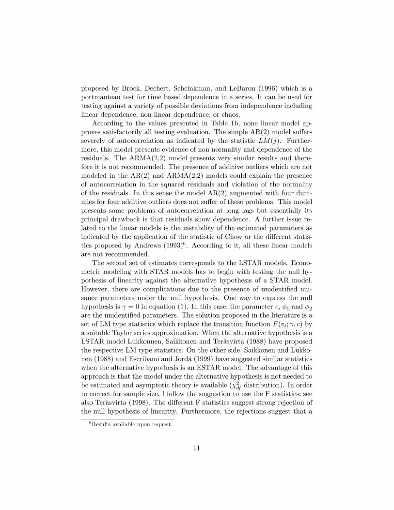
proposed by Brock, Dechert, Scheinkman, and LeBaron (1996) which is aportmanteau test for time based dependence in a series. It can be used fortesting against a variety of possible deviations from independence includinglinear dependence, non-linear dependence, or chaos.

According to the values presented in Table 1b, none linear model ap-proves satisfactorily all testing evaluation. The simple AR(2) model su¤ersseverely of autocorrelation as indicated by the statistic LM(j). Further-more, this model presents evidence of non normality and dependence of theresiduals. The ARMA(2,2) model presents very similar results and there-fore it is not recommended. The presence of additive outliers which are notmodeled in the AR(2) and ARMA(2,2) models could explain the presenceof autocorrelation in the squared residuals and violation of the normalityof the residuals. In this sense the model AR(2) augmented with four dum-mies for four additive outliers does not su¤er of these problems. This modelpresents some problems of autocorrelation at long lags but essentially itsprincipal drawback is that residuals show dependence. A further issue re-lated to the linear models is the instability of the estimated parameters asindicated by the application of the statistic of Chow or the di¤erent statis-tics proposed by Andrews (1993)6. According to it, all these linear modelsare not recommended.

The second set of estimates corresponds to the LSTAR models. Econo-metric modeling with STAR models has to begin with testing the null hy-pothesis of linearity against the alternative hypothesis of a STAR model.However, there are complications due to the presence of unidenti�ed nui-sance parameters under the null hypothesis. One way to express the nullhypothesis is = 0 in equation (1). In this case, the parameter c, �1 and �2are the unidenti�ed parameters. The solution proposed in the literature is aset of LM type statistics which replace the transition function F (vt; ; c) bya suitable Taylor series approximation. When the alternative hypothesis is aLSTAR model Lukkonnen, Saikkonen and Teräsvirta (1988) have proposedthe respective LM type statistics. On the other side, Saikkonen and Lukko-nen (1988) and Escribano and Jordá (1999) have suggested similar statisticswhen the alternative hypothesis is an ESTAR model. The advantage of thisapproach is that the model under the alternative hypothesis is not needed tobe estimated and asymptotic theory is available (�2df distribution). In orderto correct for sample size, I follow the suggestion to use the F statistics; seealso Teräsvirta (1998). The di¤erent F statistics suggest strong rejection ofthe null hypothesis of linearity. Furthermore, the rejections suggest that a

6Results available upon request.

11

LSTAR speci�cation is preferred7.Two models are presented and both include two thresholds, therefore

they are denoted by LSTAR(2). In the �rst model, the transition variableis �4yt�1 while in the second model, the variable �4yt�4 has this role.According to the estimates of , c1 and c2, the behavior of both models isnot very di¤erent. Parameter is larger in the second model which shows anabrupt switch between both regimes. Only based on the information criteria,the �rst model should be selected. This model indicates that the �rst regimeis stationary while the second one is nonstationary and persistence is higherin the �rst regimen compared to the second regime. Unlike this model, thesecond model presents roots inside of the unit circle indicating stationarity inboth regimes. Level of persistence is around 0.75 in the �rst regime of bothmodels. However, level of persistence is very low (0.09 and 0.26 in �rst andsecond model, respectively) in the second regime. It shows that duration oftransitory shocks (negative or positive) in this regime are extremely brief. Itis worth to say that for both models, roots of the autoregressive polynomialsare complex indicating pseudo-cyclical behavior.

Figure 2a shows the evolution of the transition function for the sampleperiod. The picture suggests only few periods where Peruvian economy hasexperimented very large positive and negative growth rates. The period1986:4-1987:2 re�ects the high growth rates experimented in the �rst halfof the �rst government of President A. Garcia which were associated withhigh levels of �scal spending. However, potential output does not followsame pattern of growth. Another identi�ed period is the �rst three quar-ters of 1989. The period 1994:2-1995:2 contains also observations of highgrowth rates. An important observation is that this model does not iden-tify any recession period (more than two consecutive negative growth rates)which represents a serious drawback even when information criteria sug-gests suitability. The alternative model (a LSTAR(2) model with �4yt�4as transition variable) detects some di¤erent periods. The brief periods1987:3-1988:1, 1991:3-1991:4, 1995:1-1996:2 are identi�ed as observationswhere growth rates have been particularly high. As before, the very highgrowth rates observed during government of President A. Garcia are againobtained. However, unlike previous model, the present model selects 1989:4-1990:3 as an extreme regime with negative growth rates. It is interestingand makes more sense because during these quarters the Peruvian economyexperimented negative growth rates aggravated with an hyperin�ation pe-

7The F statistics are not shown in order to save space, but they are available uponrequest.

12

riod never experimented before. Furthermore, these quarters are associatedwith high in�uence and destructive activity of the terrorism group ShinningPath.

Figure 2b show evolution of the transition function respect to the transi-tion variable and they indicate similar behavior. Figures also indicate thatobservations smaller than c1 and greater than c2 are scarce. It could suggestthat Peruvian economy has experimented a few number of observations withvery negative or positive growth rates con�rming previous obtained results.In consequence, most of observations are between both thresholds. How-ever, both estimated thresholds are (in absolute values) very large whichindicate that the interval [bc1;bc2] is broad suggesting that Peruvian econ-omy has experimented large (negative or positive) growth rates. Observingthe picture we may see that most of observations are concentrated to theright of the zero growth rate con�rming that this economy has grown in asustained way for a long period (1995-2008). Most of the observations areclearly concentrated around 0.0% and 9.0% (around 50.0%). Furthermore,comparing both pictures, the model where �4yt�4 is the transition variablepresents more abrupt change between both regimes. There is almost noobservations to the left of c1. It suggests that when economy has been inrecession times, the growth rates have been very negative but economy wasnot in this regime too much time.

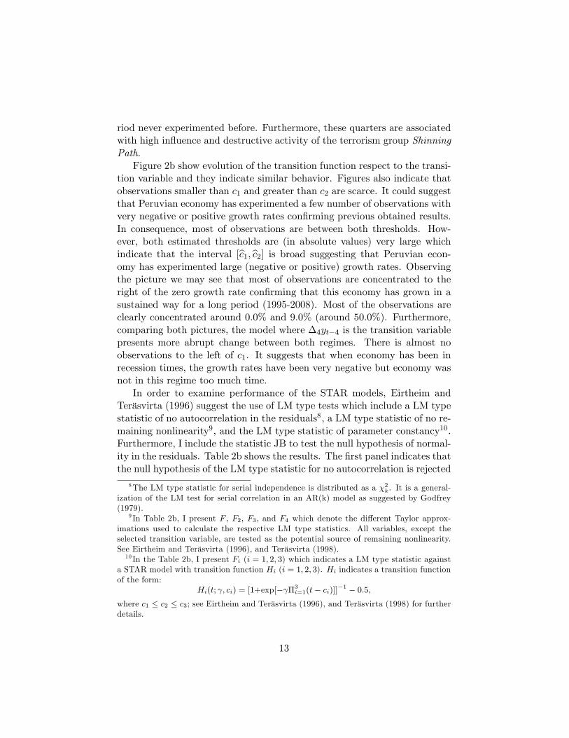
In order to examine performance of the STAR models, Eirtheim andTeräsvirta (1996) suggest the use of LM type tests which include a LM typestatistic of no autocorrelation in the residuals8, a LM type statistic of no re-maining nonlinearity9, and the LM type statistic of parameter constancy10.Furthermore, I include the statistic JB to test the null hypothesis of normal-ity in the residuals. Table 2b shows the results. The �rst panel indicates thatthe null hypothesis of the LM type statistic for no autocorrelation is rejected

8The LM type statistic for serial independence is distributed as a �2k. It is a general-ization of the LM test for serial correlation in an AR(k) model as suggested by Godfrey(1979).

9 In Table 2b, I present F , F2, F3, and F4 which denote the di¤erent Taylor approx-imations used to calculate the respective LM type statistics. All variables, except theselected transition variable, are tested as the potential source of remaining nonlinearity.See Eirtheim and Teräsvirta (1996), and Teräsvirta (1998).10 In the Table 2b, I present Fi (i = 1; 2; 3) which indicates a LM type statistic against

a STAR model with transition function Hi (i = 1; 2; 3). Hi indicates a transition functionof the form:

Hi(t; ; ci) = [1+exp[� �3i=1(t� ci)]]�1 � 0:5;where c1 � c2 � c3; see Eirtheim and Teräsvirta (1996), and Teräsvirta (1998) for furtherdetails.

13

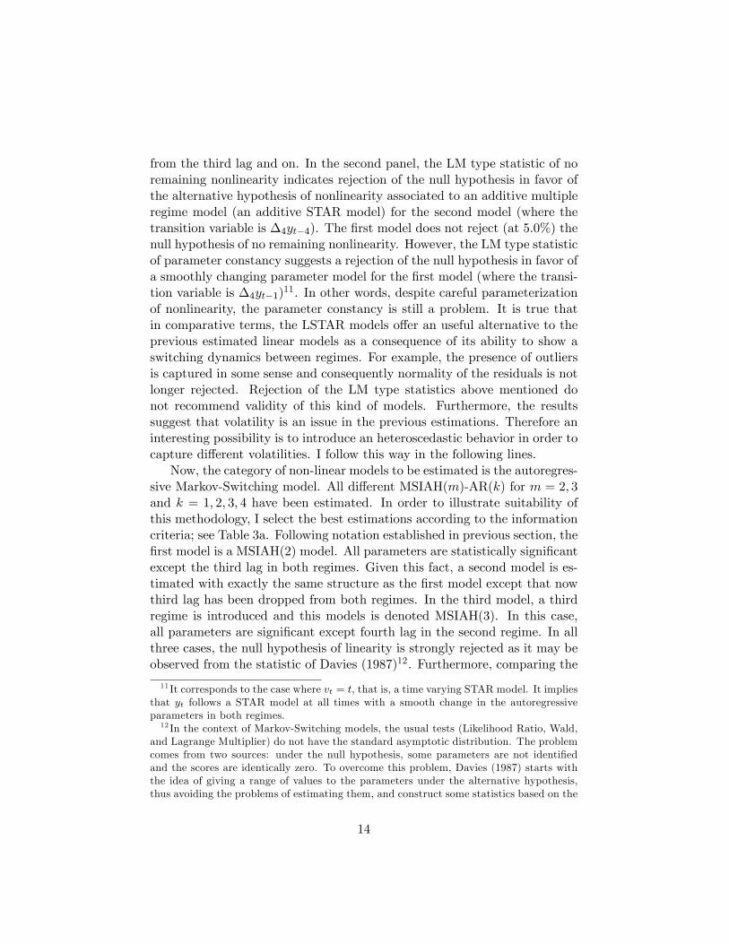
from the third lag and on. In the second panel, the LM type statistic of noremaining nonlinearity indicates rejection of the null hypothesis in favor ofthe alternative hypothesis of nonlinearity associated to an additive multipleregime model (an additive STAR model) for the second model (where thetransition variable is �4yt�4). The �rst model does not reject (at 5.0%) thenull hypothesis of no remaining nonlinearity. However, the LM type statisticof parameter constancy suggests a rejection of the null hypothesis in favor ofa smoothly changing parameter model for the �rst model (where the transi-tion variable is �4yt�1)11. In other words, despite careful parameterizationof nonlinearity, the parameter constancy is still a problem. It is true thatin comparative terms, the LSTAR models o¤er an useful alternative to theprevious estimated linear models as a consequence of its ability to show aswitching dynamics between regimes. For example, the presence of outliersis captured in some sense and consequently normality of the residuals is notlonger rejected. Rejection of the LM type statistics above mentioned donot recommend validity of this kind of models. Furthermore, the resultssuggest that volatility is an issue in the previous estimations. Therefore aninteresting possibility is to introduce an heteroscedastic behavior in order tocapture di¤erent volatilities. I follow this way in the following lines.

Now, the category of non-linear models to be estimated is the autoregres-sive Markov-Switching model. All di¤erent MSIAH(m)-AR(k) for m = 2; 3and k = 1; 2; 3; 4 have been estimated. In order to illustrate suitability ofthis methodology, I select the best estimations according to the informationcriteria; see Table 3a. Following notation established in previous section, the�rst model is a MSIAH(2) model. All parameters are statistically signi�cantexcept the third lag in both regimes. Given this fact, a second model is es-timated with exactly the same structure as the �rst model except that nowthird lag has been dropped from both regimes. In the third model, a thirdregime is introduced and this models is denoted MSIAH(3). In this case,all parameters are signi�cant except fourth lag in the second regime. In allthree cases, the null hypothesis of linearity is strongly rejected as it may beobserved from the statistic of Davies (1987)12. Furthermore, comparing the

11 It corresponds to the case where vt = t, that is, a time varying STAR model. It impliesthat yt follows a STAR model at all times with a smooth change in the autoregressiveparameters in both regimes.12 In the context of Markov-Switching models, the usual tests (Likelihood Ratio, Wald,

and Lagrange Multiplier) do not have the standard asymptotic distribution. The problemcomes from two sources: under the null hypothesis, some parameters are not identi�edand the scores are identically zero. To overcome this problem, Davies (1987) starts withthe idea of giving a range of values to the parameters under the alternative hypothesis,thus avoiding the problems of estimating them, and construct some statistics based on the

14

three models using the information criteria, the MSIAH(2) model is slightlyselected while the MSIAH(3) model is very close to it, in special accordingto the AIC.

Estimates of the standard deviation of the MSIAH(2) model suggest thatsecond regime (moderate-high growth rates) has been six times the standarddeviation of the �rst regimen (recession times). According to the MSIAH(3)model, the second regime (high growth rates) is still more volatile than the�rst regime (recessions) while last regime (moderate growth rates) presentssimilar volatility than the �rst regime (recession times). According to theset of roots implied for the AR(4) process, the �rst regime of the MSIAH(2)model appears to be nonstationary. Second regime is stationary and the levelof persistence is around 0.653. The model MSIAH(3) is also nonstationary inthe �rst regime but second and third regimes are stationary. In all cases, thepresence of complex roots assures pseudo cyclical behavior. Last Markov-Switching model (see last two columns of Table 3a) has roots inside of theunit circle indicating stationarity. The level of persistence is around 0.650in both regimes.

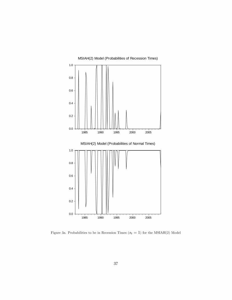
Figure 3a shows probabilities to be in recession times (st = 1) estimatedby the MSIAH(2) model. The identi�ed periods are 1985:2-1985:3, 1988:3-1988:4, 1990:2-1990:3 and 1992:2-1992:3. What is important to note is thatall these periods have a duration of only two quarters indicating very fastreverting behavior. The expected duration of the �rst regime is 1.40 quarterswhich is equivalent to 11.0% of the total number of observations. The secondregime has an expected duration of 11.95 quarters.

Another point is the fact that the model identi�es 1983:1, 1991:4 and1993:4 (only one quarters) as quarters where output presented very negativegrowth rates. Because duration is only of one quarter, they cannot be con-sidered as recession episodes according to standard or practical rules. Theseobservations may be quali�ed as outliers. For example 1983:1 is related withnatural disaster happened in the north of Peru. However, according to themodel, this only observation is an atypical growth rate but it cannot beinterpreted as part of a recession regime.

In Figure 3b, probabilities of st = 1 obtained from the alternativeMSIAH(2) are shown. The calculated expected durations are 9.35 and 12.80quarters for �rst and second regimes, respectively. It indicates that recessionand normal times have 43.8% and 56.2% of the total number of observations.

value of the objective function obtained with these given parameter values. Therefore, weobtain an upper bound for the signi�cance level of the likelihood ratio statistic under thenull hypothesis consisting of the model with the lower number of states. For further andtechnical details, see the annex of Garcia and Perron (1996).

15

In fact, the �gure shows that this model selects too many observations qual-i�ed as recession quarters. One evident case is the period 1985:2-1992:4identi�ed as a recession period which is very di¢ cult to conciliate with realdata because it has long duration and also because it includes some periodsas 1987 where economy showed high growth rates contradicting �ndings ofthe model13.

Estimates of the MSIAH(3) model indicate that the expected durationsof each regime are 1.68, 3.06 and 7.94 quarters, respectively. In terms ofthe total number of observations, it implies durations of 10.7%, 38.8%, and50.4%, respectively. Figure 3c presents the recession times (st = 1) identi-�ed by the MSIAH(3) model. According to this model, 1988:3-1988:4 and1990:2-1991:1 are observations identi�ed as recessions. The dates are inclose concordance with the real evidence. For example 1988:3-1988:4 arerelated to the negative growth rates of output related to the application of�scal-monetary policies applied in these quarters in order to stabilize highin�ation. On another side, the period 1990:2-1991:1 are quarters with neg-ative growth rates caused by the hard stabilization program applied to stophyperin�ation where monetary authority reduced strongly monetary base14.Other measures applied with the same goal were credit contraction, andunfreezing public prices. All these measures drive to the larger recession.Notice that the model does not identify negative growth rates of 1983 re-lated to the natural disaster happened in the north of Peru. Actually, themodel identi�es 1983:1 as an observation with a very negative growth ratewith high probability to be in st = 1. However, it is only one quarter andconsequently, it does not enter in the traditional and practical de�nitionof a recession of (at least) two negative consecutive growth rates. Similararguments are applied to the cases of 1987:3 and 1991:4. In other words,the model selects these observations as outliers or atypical observations butnot as recession times.

Table 3b shows di¤erent statistics to evaluate residuals of the Markov-Switching models previously estimated. First observation is that perfor-mance of all three Markov-Switching models is more satisfactory than pre-vious estimated models. The statistic LM(j) does not suggest presenceof autocorrelation in the residuals of the three models. The presence of

13 I decided to still include this model because it is a good example of a good �tting butclearly wrong in selection of the recession times (among other things). It is a very simplemodi�cation of the MSIAH(2) and it is persented in the third column of Tables 3a and3b. However this simple modi�cation shows strong changes in major results. It illustratesthat carefulness is needed at the moment of selecting models.14This program is well known as the Fujimori Plan.

16

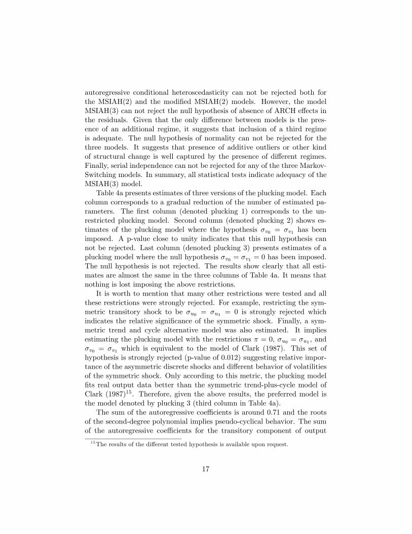
autoregressive conditional heteroscedasticity can not be rejected both forthe MSIAH(2) and the modi�ed MSIAH(2) models. However, the modelMSIAH(3) can not reject the null hypothesis of absence of ARCH e¤ects inthe residuals. Given that the only di¤erence between models is the pres-ence of an additional regime, it suggests that inclusion of a third regimeis adequate. The null hypothesis of normality can not be rejected for thethree models. It suggests that presence of additive outliers or other kindof structural change is well captured by the presence of di¤erent regimes.Finally, serial independence can not be rejected for any of the three Markov-Switching models. In summary, all statistical tests indicate adequacy of theMSIAH(3) model.

Table 4a presents estimates of three versions of the plucking model. Eachcolumn corresponds to a gradual reduction of the number of estimated pa-rameters. The �rst column (denoted plucking 1) corresponds to the un-restricted plucking model. Second column (denoted plucking 2) shows es-timates of the plucking model where the hypothesis �v0 = �v1 has beenimposed. A p-value close to unity indicates that this null hypothesis cannot be rejected. Last column (denoted plucking 3) presents estimates of aplucking model where the null hypothesis �v0 = �v1 = 0 has been imposed.The null hypothesis is not rejected. The results show clearly that all esti-mates are almost the same in the three columns of Table 4a. It means thatnothing is lost imposing the above restrictions.

It is worth to mention that many other restrictions were tested and allthese restrictions were strongly rejected. For example, restricting the sym-metric transitory shock to be �u0 = �u1 = 0 is strongly rejected whichindicates the relative signi�cance of the symmetric shock. Finally, a sym-metric trend and cycle alternative model was also estimated. It impliesestimating the plucking model with the restrictions � = 0, �u0 = �u1 , and�v0 = �v1 which is equivalent to the model of Clark (1987). This set ofhypothesis is strongly rejected (p-value of 0.012) suggesting relative impor-tance of the asymmetric discrete shocks and di¤erent behavior of volatilitiesof the symmetric shock. Only according to this metric, the plucking model�ts real output data better than the symmetric trend-plus-cycle model ofClark (1987)15. Therefore, given the above results, the preferred model isthe model denoted by plucking 3 (third column in Table 4a).

The sum of the autoregressive coe¢ cients is around 0.71 and the rootsof the second-degree polynomial implies pseudo-cyclical behavior. The sumof the autoregressive coe¢ cients for the transitory component of output

15The results of the di¤erent tested hypothesis is available upon request.

17

fall when asymmetry is accounted for, and thus it tends to be statisticallylower in the plucking model than in the model of Clark, for example (0.92).According to Simone de Nadal and Clarke (2007), it is important because ifthe sum of the autoregressive coe¢ cients is close to one, output shocks couldbe erroneously considered as permanent (or very persistent) if estimatedoutput behavior is restricted to be symmetric when it is in fact asymmetric.

Therefore, the estimates also indicate that once a negative transitoryshock hits the economy, its e¤ects decay relatively fast, as indicated by therelatively low value of the sum of the autoregressive coe¢ cients. This resultis also found in previous empirical research as Kim and Nelson (1999), Millsand Wang (2001), Rodríguez (2005), Nadal de Simone and Clarke (2007).

Regarding the asymmetric shock (�), it is negative as expected in allcolumns of the Table 4a. The asymmetric shock appears to explain moreof the variance of the cyclical component than the symmetric shock. Ourestimates also indicate that the stochastic trend component is not a¤ected bysigni�cant permanent �normal� (�v0) or recessive (�v1) shocks. Observingthe estimates of Table 4a, we �nd that these parameters are not statisticallysigni�cant and therefore they are deleted in �nal third column of Table 4a.However, accounting for asymmetry, makes the shock to the trend growth(�w) component statistically signi�cant16.

Figure 4a shows the evolution of the current and potential output and thecorresponding estimated cycles according to the preferred plucking model(plucking 3). The data seem to con�rm Friedman�s view that the economyis most of the time at its potential level (since 1994-1995) but the evidencedoes not show that output is plucked down from time to time. What weobserve is a very large period where output appears to be plucked down andafter it, a long period where economy is close to the potential output.

Figure 4b presents the probabilities to be in recession times related to theselected plucking model (plucking 3). Of course, evolution of these probabil-ities are strongly correlated with the previous picture. The model suggeststhat 1988, 1993, 1994 are periods where economy has been in recession timesor in a very low growth rates regime. For the previous years, the probabili-

16Strictly speaking, the plucking model (and also the model of Clark (1987)) speci�esthe real output as an I(2) process. It is well known, however, that real output is a trendstationary process or an I(1) process. If the variance of the shock to the trend growthcomponent is not statistically di¤erent from zero or it is very small, this should not pose amajor misspeci�cation problems. In our case, this parameter is statistically signi�cant butis always a small value. It should not pose major misspeci�cations problems. All modelswere estimated without restricting growth to have zero variance. In fact, when model wasestimated imposing this restriction, a strong rejection was obtained.

18

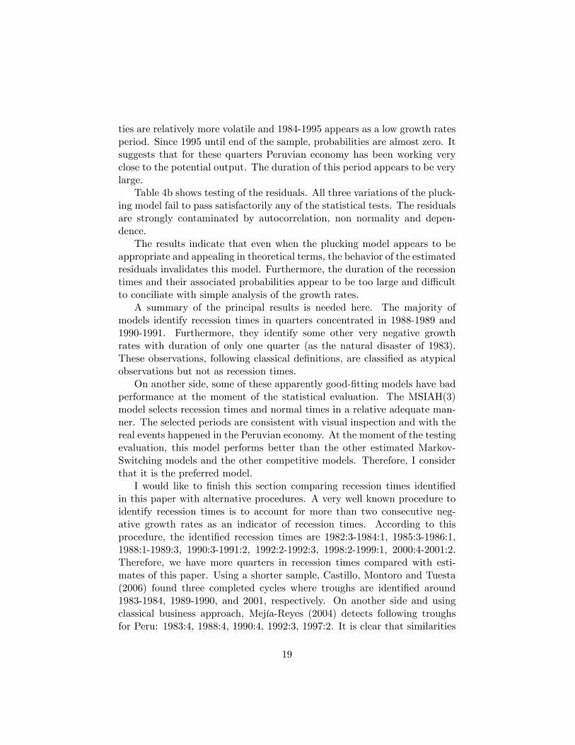
ties are relatively more volatile and 1984-1995 appears as a low growth ratesperiod. Since 1995 until end of the sample, probabilities are almost zero. Itsuggests that for these quarters Peruvian economy has been working veryclose to the potential output. The duration of this period appears to be verylarge.

Table 4b shows testing of the residuals. All three variations of the pluck-ing model fail to pass satisfactorily any of the statistical tests. The residualsare strongly contaminated by autocorrelation, non normality and depen-dence.

The results indicate that even when the plucking model appears to beappropriate and appealing in theoretical terms, the behavior of the estimatedresiduals invalidates this model. Furthermore, the duration of the recessiontimes and their associated probabilities appear to be too large and di¢ cultto conciliate with simple analysis of the growth rates.

A summary of the principal results is needed here. The majority ofmodels identify recession times in quarters concentrated in 1988-1989 and1990-1991. Furthermore, they identify some other very negative growthrates with duration of only one quarter (as the natural disaster of 1983).These observations, following classical de�nitions, are classi�ed as atypicalobservations but not as recession times.

On another side, some of these apparently good-�tting models have badperformance at the moment of the statistical evaluation. The MSIAH(3)model selects recession times and normal times in a relative adequate man-ner. The selected periods are consistent with visual inspection and with thereal events happened in the Peruvian economy. At the moment of the testingevaluation, this model performs better than the other estimated Markov-Switching models and the other competitive models. Therefore, I considerthat it is the preferred model.

I would like to �nish this section comparing recession times identi�edin this paper with alternative procedures. A very well known procedure toidentify recession times is to account for more than two consecutive neg-ative growth rates as an indicator of recession times. According to thisprocedure, the identi�ed recession times are 1982:3-1984:1, 1985:3-1986:1,1988:1-1989:3, 1990:3-1991:2, 1992:2-1992:3, 1998:2-1999:1, 2000:4-2001:2.Therefore, we have more quarters in recession times compared with esti-mates of this paper. Using a shorter sample, Castillo, Montoro and Tuesta(2006) found three completed cycles where troughs are identi�ed around1983-1984, 1989-1990, and 2001, respectively. On another side and usingclassical business approach, Mejía-Reyes (2004) detects following troughsfor Peru: 1983:4, 1988:4, 1990:4, 1992:3, 1997:2. It is clear that similarities

19

exist in the selection of the recession times. More speci�cally, we may saythat dates of recession times identi�ed in this paper are included in the morelarge number of recession times identi�ed for other alternative procedures.

A natural question is to know reasons why the methods applied in thispaper select a reduced number of recession times. Or why the other methodscould overestimate the number of quarters of recession times. My conjec-ture is that Peruvian economy has experimented very negative (and verypositive) growth rates which could a¤ect the selection of recession times byany method. The estimated non-linear models correctly identify these ob-servation but they are quali�ed as atypical observations. From another side,because there are very negative growth rates, moderate negative growthrates could not be selected as recession times. For example, the naturaldisaster of 1983 a¤ected seriously agricultural sector and consequently realoutput. However, this phenomenon is selected as an atypical observationbecause it has one quarter of duration. The only explanation for this fact isthat, even when growth rates around 1983 are highly negative, these ratesare smaller compared to the extreme values experimented in other momentsof the economy. Another example could be the �nancial crises in Asia andRussia. Apparently, these events have a¤ected economy. However the neg-ative growth rates are smaller compared with other negative growth ratesexperimented for the economy. Therefore, the negative growth rates causedby external �nancial crises are not detected because they are �small�.

4 Conclusions

In order to identify and analyze business cycles, three alternative non-linear models have been estimated. The �rst class is the Logistic SmoothTransition Autoregressive (LSTAR) model suggested by Teräsvirta (1994)where one observable variable drives the switching behavior between the tworegimes. The second model is an extended version of the Markov-Switchingmodel proposed by Hamilton (1989) where an unobservable variable deter-mines the switching behavior between m regimes in a probabilistic way. Thethird model is the unobserved components model theoretically suggested byFriedman (1964, 1993) and econometrically speci�ed by Kim and Nelson(1999). The new feature of this model is the presence of an asymmetricshock that explain the presence of recession times. In the rest of the time,economy is operating close to the potential output.

The majority of the estimated models identify periods of recessions asquarters concentrated around 1988 and 1990. Some events as the natural

20

disasters happened in 1983 are only captured as atypical observations butthey do not qualify as recession times. Furthermore, the Asian and Russian�nancial crises are not identi�ed as recession times. It means that theseevents probably a¤ected the �nancial sector of the economy but not a¤ectedthe real output of the economy. Another alternative explanation is that thenegative e¤ects of these events were smaller compared to the negative impactof other events. The alternative hypothesis that armed and destructiveactions of the terrorist group Shining Path could cause recession periods isdi¢ cult to accept according to the quantitative results.

Another similarity between models is that since 1994-1995 until end ofthe sample, the economy appears to enter in a period of relative sustainablegrowth. It is supported by the various structural reforms applied in the labormarket, �nancial sector, external sector, and the adoption of the targetingin�ation system. All these measures contributed to the adequate behaviorof the economy since 1995 with less volatility in the evolution of the majormacroeconomic variables. Therefore, all non-linear models identify a longduration regime characterized by moderate-high growth rates.

From the point of view of the statistical evaluation of the di¤erent non-linear models, the MSIAH(3) model shows superior performance. Thismodel selects the recession times and normal times in a relative adequatemanner. The selected periods are consistent with visual inspection andwith the real events happened in the Peruvian economy. At the moment ofthe testing evaluation, the model performs better than the other Markov-Switching models and the other competitive models. The model does notpresent evidence of autocorrelation in the residuals and the squared resid-uals. Furthermore, there is no presence of non normality, and the residualsare independent.

References

[1] Andrews, D. W. K. (1993), �Testing for Parameter Instability andStructural Change with Unknown Change Point,� Econometrica 61(4), 821-856.

[2] Aigner, D., A. K. Lovell, and P. Schmidt (1977), �Formulations and Es-timation of Stochastic Frontier Production Models,�Journal of Econo-metrics 6, 21-37.

21

[3] Bodman, P. M., and M. Crosby (2000), �Phases of the Canadian Busi-ness Cycle�, Canadian Journal of Economics 33, 618-633.

[4] Brock, W. A., W. D. Dechert, J. A. Scheinkman, and B. LeBaron(1996), �A Test for Independence Based on the Correlation Dimen-sion,�Econometric Reviews 15, 197-235.

[5] Castillo, P., C. Montoro, and V. Tuesta (2006), �Hechos Estilizados dela Economía Peruana,�Working Paper 2006-05, Central Bank of Peru.

[6] Clark, P. (1987), �The Cyclical Component of US Economic Activity,�Quarterly Journal of Economics 102, 797-814.

[7] Davies, R. B. (1987), �Hypothesis Testing when a Nuisance ParameterIs Present Only Under the Alternative,�Biometrika 74, 33-43.

[8] Delong, J. B., and L. H. Summers (1986), �Are Business Cycles Sym-metrical?,� in Gordon, R. (ed.), American Business Cycle: Continuityand Change, 166-179. Chicago: University of Chicago Press.

[9] Eitrheim, O., and T. Teräsvirta (1996), �Testing the Adequacy ofSmooth Transition Autoregressive Models,� Journal of Econometrics74, 56-75.

[10] Escribano, A. and O. Jordá (1999), �Improved Testing and Speci�cationof Smooth Transition Regression Models,� in P. Rothman (ed.), Non-linear Time Series Analysis of Economic and Financial Data, Boston:Kluwer, 289�319.

[11] Falk, B. (1986), �Further Evidence on the Asymmetric Behavior ofEconomic Time Series over the Business Cycle,� Journal of PoliticalEconomy 94:5, 1096-1109.

[12] Friedman, M. (1964), �Monetary Studies of the National Bureau,�TheNational Bureau Enters Its 45th Year, 44th Annual Report, 7-25.

[13] Friedman, M. (1993), �The �Plucking Model�of Business Fluctuationsrevisited,�Economic Inquiry, 171-177.

[14] Galvão, A. B. C. (2002), �Can Non-Linear Time Series Models GenerateUS Business Cycle Asymmetric Shape,�Economic Letters 77, 187-194.

[15] Garcia, R., and P. Perron (1996), �An Analysis of the Real InterestRate Under Regime Shifts,�The Review of Economics and Statistics78(1), 111-125.

22

[16] Godfrey, L. G. (1979), �Testing the Adequacy of a Time Series Model�,Biometrika 66, 67-72.

[17] Goodwin T. H. (1993), �Business-Cycle Analysis with a Markov-Switching Model� Journal of Business and Economic Statistics 11,331-339.

[18] Goodwin, T. H., and R. J. Sweeney (1993), �International Evidence onFriedman�s Theory of the Business Cycle,�Economic Inquiry, 178-193.

[19] Granger, C. W. J., and T. Teräsvirta (1993), Modeling Nonlinear Eco-nomic Relationships, New York: Oxford University Press.

[20] Hamilton, J. D. (1989), �A New approach to the Economic Analysisof Nonstationarity Time Series and the Business Cycle,�Econometrica57, 357-384.

[21] Hendry, D. F., and H.-M. Krolzig (2001), Automatic Econometric ModelSelection using PcGets, London: Timberlake Consultants Ltd.

[22] Jansen, E. S. and, T. Teräsvirta (1996), �Testing parameter constancyand superexogeneity in econometric equations,�Oxford Bulletin of Eco-nomics and Statistics 58, 735�768.

[23] Keynes, J. M. (1936), The General Theory of Employment, Interest,and Money, London: MacMillan.

[24] Kim, Ch.-J., and Ch. R. Nelson (1999), �Friedman�s Plucking Modelof Business Fluctuations: Tests and Estimates of Permanent and Tran-sitory Components,� Journal of Money Credit, and Banking 31 (3),317-334.

[25] Krolzig, H.-M. (1997), Markov-Switching Vector Autoregressions. Mod-elling, Statistical Inference, and Application to Business Cycle Analysis,Lecture Notes in Economics and Mathematical Systems, Volume 454,Berlin: Springer.

[26] Lin, C.F.J. and T. Teräsvirta (1994), �Testing the Constancy of Re-gression Parameters Against Continuous Structural Change,� Journalof Econometrics 62, 211-228.

[27] Luukkonen, R., P. Saikkonen, and T. Teräsvirta (1988), �Testing Lin-earity against Smooth Transition Autoregressive Models,�Biometrika75, 491�499.

23

[28] Mejía-Reyes, P. (2004), �Classical Business Cycles in America: AreNational Business Cycles Synchronized?,�International Journal of Ap-plied Econometrics and Quantitative Studies 3, 75-102.

[29] Mills, T. C., and P. Wang (2002), �Plucking Models of Business CycleFluctuations: Evidence from the G-7 Countries,�Empirical Economics25, 225-276

[30] Mitchell, W. (1927), Business Cycles: The Problem and Its Setting,New York: National Bureau of Economic Research.

[31] Nadal De Simone, F., and S. Clarke (2007), �Asymmetry in BusinessFluctuations: International Evidence on Friedman�s Plucking Model,�Journal of International Money and Finance 26, 64-85.

[32] Neftci, S. N. (1984), �Are Economic Time Series Asymmetric Over theBusiness Cycles?,�Journal of Political Economy 92 (2), 307-328.

[33] Rodríguez, G. (2005), �Estimates of Permanent and Transitory Com-ponents for Canadian Regions using the Friedman�s Plucking Model ofBusiness Fluctuations,�Canadian Journal of Regional Science 27 (1),61-78.

[34] Rodríguez, G. (2010a), �Using A Forward-Looking Phillips Curve toEstimate the Output Gap in Peru,� forthcoming in Review of AppliedEconomics.

[35] Rodríguez, G. (2010b), �Estimating Output Gap, Core In�ation, andthe NAIRU for Peru,�forthcoming in Applied Econometrics and Inter-national Development .

[36] Saikkonen, P., and R. Luukkonen (1988), �Lagrange Multiplier Testsfor Testing Nonlinearity in Time Series Models,�Scandinavian Journalof Statistics 58, 601-613.

[37] Sichel, D. E. (1993), �Business Cycle Asymmetry: A Deeper Look,�Economic Inquiry, 224-236.

[38] Teräsvirta, T. (1994), �Speci�cation, Estimation, and Evaluation ofSmooth Transition Autoregressive Models,� Journal of the AmericanStatistical Association 89, 208�218.

[39] Teräsvirta, T. (1998), �Modelling Economic Relationships with SmoothTransition Regressions,�in A. Ullah and D. E. A. Giles (eds.), Handbookof Applied Economic Statistics, New York: Marcel Dekker, 507�552.

24

[40] Teräsvirta, T. and H. M. Anderson (1992), �Characterizing Nonlinear-ities in Business Cycles using Smooth Transition Autoregressive Mod-els,�Journal of Applied Econometrics 7, S119�S136.

[41] Teräsvirta, T., D. Tjøstheim, and C. W. J. Granger (1994), �Aspects ofModelling Nonlinear Time Series,�in R. F. Engle and D. L. McFadden(eds.), Handbook of Econometrics, Volume IV, Amsterdam: ElsevierScience, 2917�2957.

[42] van Dijk, D., T. Teräsvirta, and P. H. Franses (2002), �Smooth Transi-tion Autoregressive Models. A Survey of Recent Developments,�Econo-metric Reviews 21, 1-47.

[43] Watson, M. W. (1986), �Univariate Detrending Methods with Stochas-tic Trends,�Journal of Monetary Economics 18, 29-75.

25

Table 1a. Estimates of Linear Models

Coe¢ cient AR(2) ARMA(2,2) AR(2) + Additive Outliers

Estimate (p-value) Estimate (p-value) Estimate (p-value)

c 0.008 (0.078) 0.012 (0.058) 0.009 (0.005)

�1 1.184 (0.000) 1.056 (0.000) 1.006 (0.000)

�2 -0.479 (0.000) -0.516 (0.000)

�3 -0.382 (0.000)

�1�2 0.452 (0.000)

DU1t -0.137 (0.000)

DU2t -0.199 (0.000)

DU3t -0.192 (0.000)

DU4t -0.153 (0.000)

Other Information

R2

0.718 0.722 0.833

AIC -3.437 -3.443 -3.924

HQ -3.407 -3.402 -3.854

SC -3.363 -3.343 -3.750

DU1t= 1 if t = 1988 : 4, DU2t= 1 if t = 1990 : 2, DU3t= 1 if t = 1990 : 3,DU4t= 1 if t = 1991 : 4

26

Table 1b. Evaluation of Linear Models

Statistic AR(2) ARMA(2,2) AR(2) + Additive Outliers

Value (p-value) Value (p-value) Value (p-value)

LM Test for Autocorrelation in Residuals

LM(1) 0.098 (0.754) 5.724 (0.018) 1.379 (0.243)

LM(2) 0.499 (0.608) 7.038 (0.001) 0.825 (0.441)

LM(3) 4.325 (0.006) 5.485 (0.002) 2.175 (0.096)

LM(4) 5.658 (0.000) 4.443 (0.002) 2.832 (0.028)

LM(8) 2.935 (0.006) 2.797 (0.008) 2.734 (0.009)

Autoregressive Conditional Heteroscedasticity in Residuals

ARCH(1) 16.847 (0.000) 22.611 (0.000) 0.356 (0.552)

ARCH(2) 8.283 (0.000) 11.386 (0.000) 0.321 (0.726)

Normality Test of Residuals

JB 38.580 (0.000) 70.029 (0.000) 0.379 (0.827)

Independence Test of Residuals

BDS(m=2,0.7) 3.363 (0.000) 3.998 (0.000) 0.953 (0.340)

BDS(m=3,0.7) 4.386 (0.000) 5.099 (0.000) 1.431 (0.152)

BDS(m=4,0.7) 5.007 (0.000) 6.004 (0.000) 1.738 (0.082)

BDS(m=5,0.7) 5.321 (0.000) 6.332 (0.000) 2.371 (0.018)

BDS(m=6,0.7) 6.237 (0.000) 6.765 (0.000) 3.064 (0.002)

The statistic LM(j) tests the null hypothesis of no autocorrelation of order j in theresiduals; ARCH(j) tests the presence of Autoregressive conditional heteroscedasticity inthe residuals; JB is the Jarque and Bera statistic to test the null hypothesis of normality

in residuals; and BDS tests the null hypothesis of independence in residuals.

27

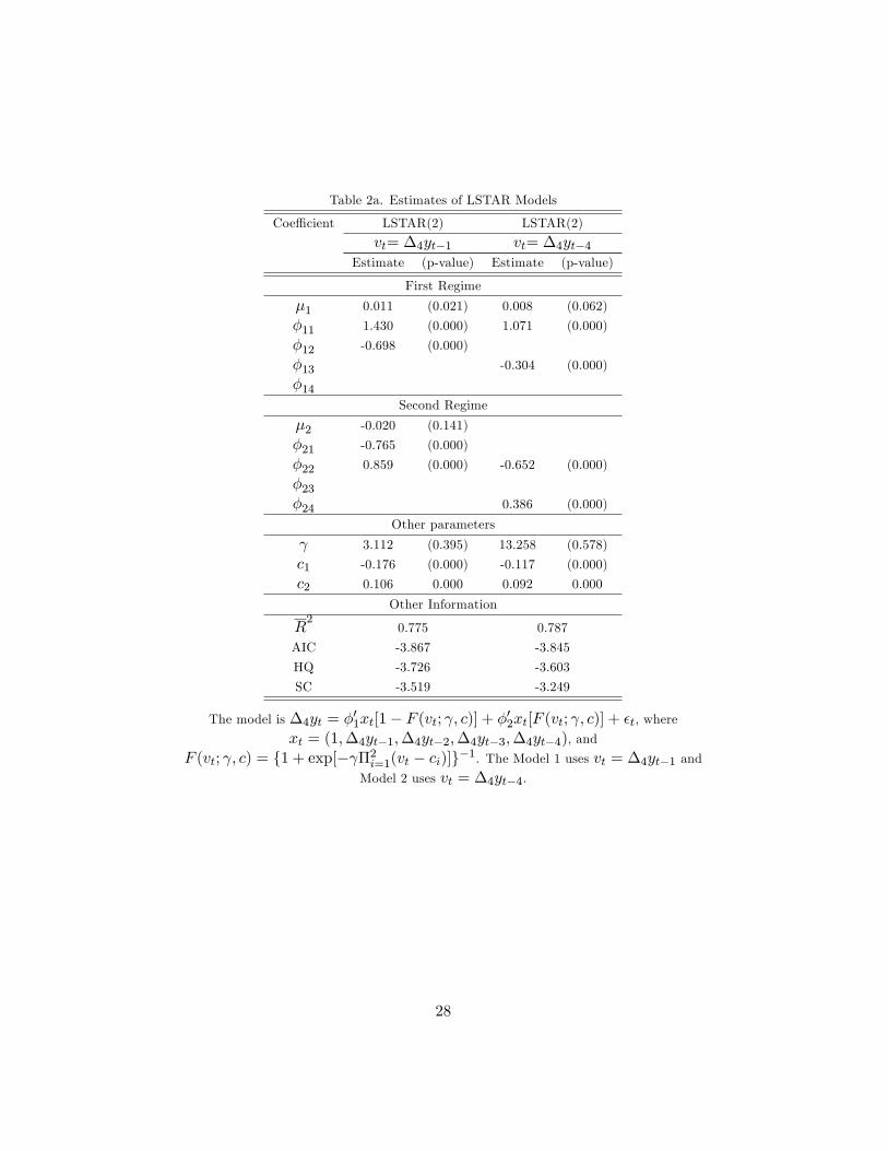
Table 2a. Estimates of LSTAR Models

Coe¢ cient LSTAR(2) LSTAR(2)

vt= �4yt�1 vt= �4yt�4Estimate (p-value) Estimate (p-value)

First Regime

�1 0.011 (0.021) 0.008 (0.062)

�11 1.430 (0.000) 1.071 (0.000)

�12 -0.698 (0.000)

�13 -0.304 (0.000)

�14Second Regime

�2 -0.020 (0.141)

�21 -0.765 (0.000)

�22 0.859 (0.000) -0.652 (0.000)

�23�24 0.386 (0.000)

Other parameters

3.112 (0.395) 13.258 (0.578)

c1 -0.176 (0.000) -0.117 (0.000)

c2 0.106 0.000 0.092 0.000

Other Information

R2

0.775 0.787

AIC -3.867 -3.845

HQ -3.726 -3.603

SC -3.519 -3.249

The model is �4yt = �01xt[1� F (vt; ; c)] + �02xt[F (vt; ; c)] + �t, where

xt = (1;�4yt�1;�4yt�2;�4yt�3;�4yt�4), andF (vt; ; c) = f1 + exp[� �2i=1(vt � ci)]g�1. The Model 1 uses vt = �4yt�1 and

Model 2 uses vt = �4yt�4.

28

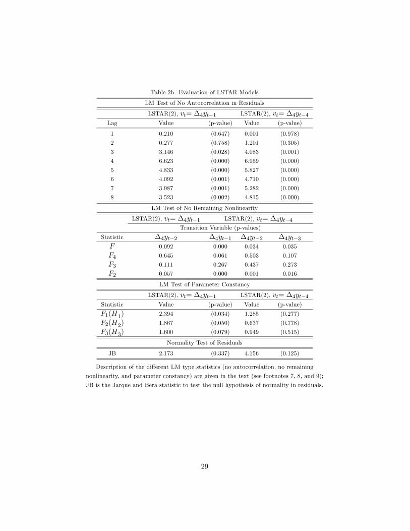
Table 2b. Evaluation of LSTAR Models

LM Test of No Autocorrelation in Residuals

LSTAR(2), vt= �4yt�1 LSTAR(2), vt= �4yt�4Lag Value (p-value) Value (p-value)

1 0.210 (0.647) 0.001 (0.978)

2 0.277 (0.758) 1.201 (0.305)

3 3.146 (0.028) 4.083 (0.001)

4 6.623 (0.000) 6.959 (0.000)

5 4.833 (0.000) 5.827 (0.000)

6 4.092 (0.001) 4.710 (0.000)

7 3.987 (0.001) 5.282 (0.000)

8 3.523 (0.002) 4.815 (0.000)

LM Test of No Remaining Nonlinearity

LSTAR(2), vt= �4yt�1 LSTAR(2), vt= �4yt�4Transition Variable (p-values)

Statistic �4yt�2 �4yt�1 �4yt�2 �4yt�3F 0.092 0.000 0.034 0.035

F4 0.645 0.061 0.503 0.107

F3 0.111 0.267 0.437 0.273

F2 0.057 0.000 0.001 0.016

LM Test of Parameter Constancy

LSTAR(2), vt= �4yt�1 LSTAR(2), vt= �4yt�4Statistic Value (p-value) Value (p-value)

F1(H1) 2.394 (0.034) 1.285 (0.277)

F2(H2) 1.867 (0.050) 0.637 (0.778)

F3(H3) 1.600 (0.079) 0.949 (0.515)


JB 2.173 (0.337) 4.156 (0.125)

Description of the di¤erent LM type statistics (no autocorrelation, no remaining

nonlinearity, and parameter constancy) are given in the text (see footnotes 7, 8, and 9);

JB is the Jarque and Bera statistic to test the null hypothesis of normality in residuals.

29

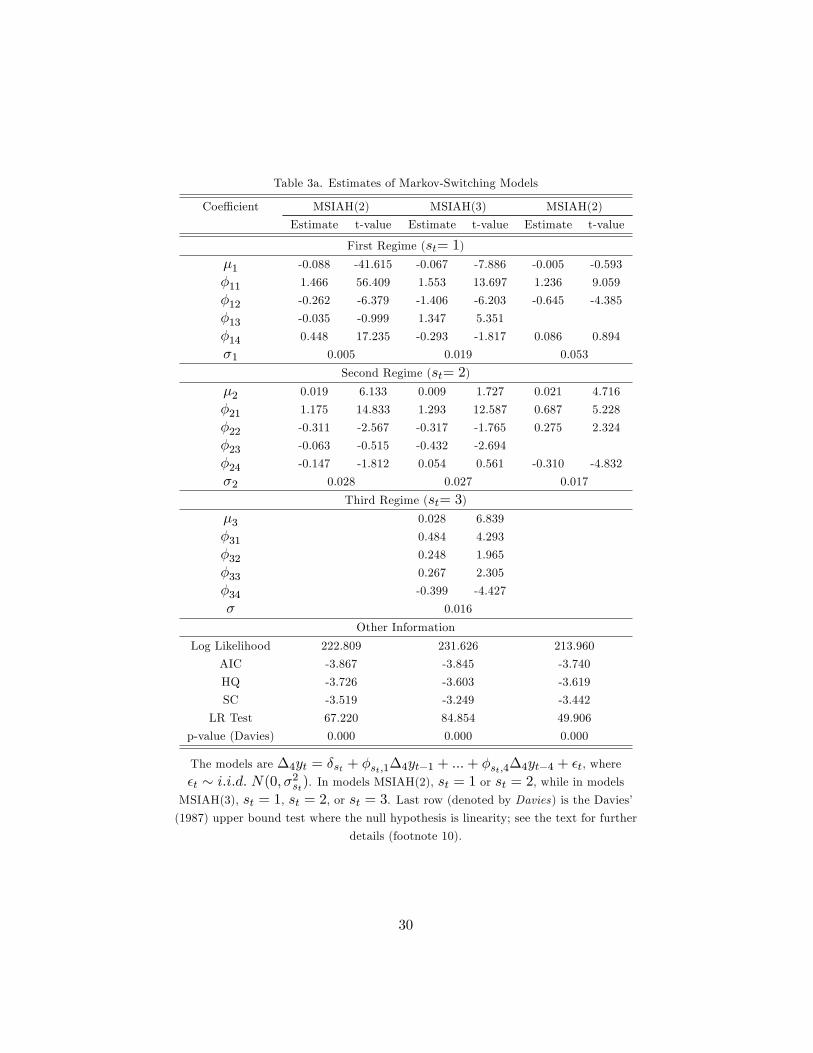
Table 3a. Estimates of Markov-Switching Models

Coe¢ cient MSIAH(2) MSIAH(3) MSIAH(2)

Estimate t-value Estimate t-value Estimate t-value

First Regime (st= 1)

�1 -0.088 -41.615 -0.067 -7.886 -0.005 -0.593

�11 1.466 56.409 1.553 13.697 1.236 9.059

�12 -0.262 -6.379 -1.406 -6.203 -0.645 -4.385

�13 -0.035 -0.999 1.347 5.351

�14 0.448 17.235 -0.293 -1.817 0.086 0.894

�1 0.005 0.019 0.053

Second Regime (st= 2)

�2 0.019 6.133 0.009 1.727 0.021 4.716

�21 1.175 14.833 1.293 12.587 0.687 5.228

�22 -0.311 -2.567 -0.317 -1.765 0.275 2.324

�23 -0.063 -0.515 -0.432 -2.694

�24 -0.147 -1.812 0.054 0.561 -0.310 -4.832

�2 0.028 0.027 0.017

Third Regime (st= 3)

�3 0.028 6.839

�31 0.484 4.293

�32 0.248 1.965

�33 0.267 2.305

�34 -0.399 -4.427

� 0.016

Other Information

Log Likelihood 222.809 231.626 213.960

AIC -3.867 -3.845 -3.740

HQ -3.726 -3.603 -3.619

SC -3.519 -3.249 -3.442

LR Test 67.220 84.854 49.906

p-value (Davies) 0.000 0.000 0.000

The models are �4yt = �st + �st;1�4yt�1 + :::+ �st;4�4yt�4 + �t, where�t � i:i:d: N(0; �2st). In models MSIAH(2), st = 1 or st = 2, while in modelsMSIAH(3), st = 1, st = 2, or st = 3. Last row (denoted by Davies) is the Davies�(1987) upper bound test where the null hypothesis is linearity; see the text for further

details (footnote 10).

30

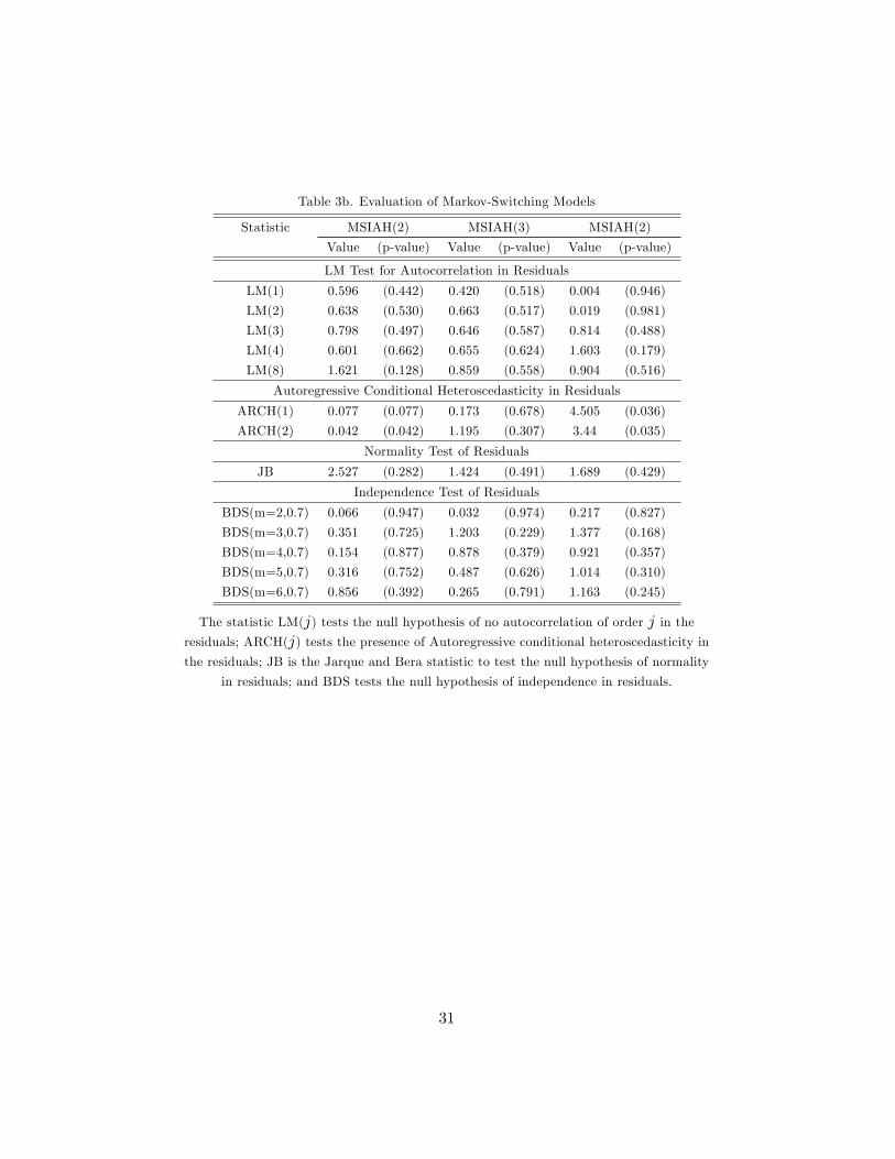
Table 3b. Evaluation of Markov-Switching Models

Statistic MSIAH(2) MSIAH(3) MSIAH(2)



LM(1) 0.596 (0.442) 0.420 (0.518) 0.004 (0.946)

LM(2) 0.638 (0.530) 0.663 (0.517) 0.019 (0.981)

LM(3) 0.798 (0.497) 0.646 (0.587) 0.814 (0.488)

LM(4) 0.601 (0.662) 0.655 (0.624) 1.603 (0.179)

LM(8) 1.621 (0.128) 0.859 (0.558) 0.904 (0.516)


ARCH(1) 0.077 (0.077) 0.173 (0.678) 4.505 (0.036)

ARCH(2) 0.042 (0.042) 1.195 (0.307) 3.44 (0.035)


JB 2.527 (0.282) 1.424 (0.491) 1.689 (0.429)


BDS(m=2,0.7) 0.066 (0.947) 0.032 (0.974) 0.217 (0.827)

BDS(m=3,0.7) 0.351 (0.725) 1.203 (0.229) 1.377 (0.168)

BDS(m=4,0.7) 0.154 (0.877) 0.878 (0.379) 0.921 (0.357)

BDS(m=5,0.7) 0.316 (0.752) 0.487 (0.626) 1.014 (0.310)

BDS(m=6,0.7) 0.856 (0.392) 0.265 (0.791) 1.163 (0.245)



31

Table 4a. Estimates of Plucking Models

Coe¢ cient Plucking 1 Plucking 2 Plucking 3

Estimate t-value Estimate t-value Estimate t-value

q 0.94420 27.218 0.94421 27.368 0.9442 27.368

p 0.97519 54.971 0.97519 55.095 0.9752 55.096

�1 0.96407 10.124 0.96408 10.105 0.9641 10.095

�2 -0.25342 -2.993 -0.25343 -2.995 �0.2534 -2.984

�u0 0.01210 11.634 0.01210 12.100 0.0121 12.100

�u1 0.03497 8.699 0.03497 8.742 0.0349 8.725

�v0 0.00002 0.031 0.00005 0.038

�v1 0.00016 0.024

�w 0.00173 2.790 0.00173 2.883 0.0017 2.833

� -0.05367 -5.329 -0.05366 -5.366 -0.0537 -5.370

Log Likelihood 249.809 249.809 249.809

The complete speci�cation of the model is given by expressions (5)-(16) in the text.

32

Table 4b. Evaluation of Plucking Models

Statistic Plucking 1 Plucking 2 Plucking 3



LM(1) 42.654 (0.000) 42.652 (0.000) 42.654 (0.000)

LM(2) 21.438 (0.000) 21.431 (0.000) 21.438 (0.000)

LM(3) 15.587 (0.000) 15.586 (0.000) 15.587 (0.000)

LM(4) 11.583 (0.000) 11.583 (0.000) 11.583 (0.000)

LM(8) 7.489 (0.000) 7.488 (0.000) 7.489 (0.000)


ARCH(1) 30.148 (0.000) 30.149 (0.000) 30.148 (0.000)

ARCH(2) 19.189 (0.000) 19.189 (0.000) 19.189 (0.000)


JB 175.912 (0.000) 175.906 (0.000) 175.904 (0.000)


BDS(m=2,0.7) 5.334 (0.000) 5.334 (0.000) 5.334 (0.000)

BDS(m=3,0.7) 7.297 (0.000) 7.297 (0.000) 7.297 (0.000)

BDS(m=4,0.7) 8.461 (0.000) 8.461 (0.000) 8.461 (0.000)

BDS(m=5,0.7) 9.614 (0.000) 9.614 (0.000) 9.614 (0.000)

BDS(m=6,0.7) 10.713 (0.000) 10.713 (0.000) 10.713 (0.000)



33

9.8

10.0

10.2

10.4

10.6

10.8

11.0

1985 1990 1995 2000 2005

Logarithm of the NonSeasonal Adjusted Real Output

.3

.2

.1

.0

.1

.2

1985 1990 1995 2000 2005

Annual Growth rates

Figure 1. Logarithm of the Non-Seasonal Adjusted Real Output and Annual Growth

Rates

34

0.0

0.2

0.4

0.6

0.8

1.0

1985 1990 1995 2000 2005

LSTAR(2) Model (version 1)

0.0

0.2

0.4

0.6

0.8

1.0

1985 1990 1995 2000 2005


Figure 2a. Transition Function against Time; LSTAR(2) model with Transition Variable

�4yt�1 (version 1) and LSTAR(2) model with Transition Variable �4yt�4 (version 2)

35

0.0

0.2

0.4

0.6

0.8

1.0

.3 .2 .1 .0 .1 .2

Transition Variable

Tran

sitio

nFu

nctio

n

0.0

0.2

0.4

0.6

0.8

1.0

.3 .2 .1 .0 .1 .2

Transition Variable

Tran

sitio

nFu

nctio

n



Figure 2b. Transition Function against Transition Variable; LSTAR(2) model with

Transition Variable �4yt�1 (version 1) and LSTAR(2) model with Transition Variable�4yt�4 (version 2)

36

0.0

0.2

0.4

0.6

0.8

1.0

1985 1990 1995 2000 2005

MSIAH(2) Model (Probabilities of Recession Times)

0.0

0.2

0.4

0.6

0.8

1.0

1985 1990 1995 2000 2005

MSIAH(2) Model (Probabilities of Normal Times)

Figure 3a. Probabilities to be in Recession Times (st = 1) for the MSIAH(2) Model

37

0.0

0.2

0.4

0.6

0.8

1.0

1985 1990 1995 2000 2005

Alternative MSIAH(2) Model (Probabilities of Recession Times)

0.0

0.2

0.4

0.6

0.8

1.0

1985 1990 1995 2000 2005

Alternative MSIAH(2) Model (Probabilities of Normal Times)

Figure 3b. Probabilities to be in Recession Times (st = 1)and Normal Times (st = 2)for the Alternative MSIAH(2) Model

38

0.0

0.2

0.4

0.6

0.8

1.0

85 90 95 00 05

MSIAH(3) Model (Probabilities of Recession Times)

0.0

0.2

0.4

0.6

0.8

1.0

85 90 95 00 05

MSIAH(3) Model (Probabilit ies of High Growth Times)

0.0

0.2

0.4

0.6

0.8

1.0

85 90 95 00 05

MSIAH(3) Model (Probabilit ies of Normal Times)

Figure 3c. Probabilities to be in Recession Times (st = 1), High Hrowth Times((st = 2), and Normal Times (st = 3) for the MSIAH(3) Model

39

9.8

10.0

10.2

10.4

10.6

10.8

11.0

1985 1990 1995 2000 2005Real OutputPotential Real Output (plucking 3)

.30

.25

.20

.15

.10

.05

.00

.05

1985 1990 1995 2000 2005

Cycle (plucking 3)

Figure 4a. Real Output and Potential Real Output of the selected Plucking Model

(plucking 3); Transitory Component of the selected Plucking Model (plucking 3)

40

0.0

0.2

0.4

0.6

0.8

1.0

82 84 86 88 90 92 94 96 98 00 02 04 06 08

Probabilities of Recession Times (plucking 3)

Figure 4b. Probabilities to be in Recession Times (st= 1) of the selected PluckingModel (plucking 3)

41

Documents

DOCUMENTO DE TRABAJO N° 284 UNIVERSIDAD · PDF [email protected]. 1 (1989). In his original paper, Hamilton used an AR(4) speci–cation in or