Documentation of a Spreadsheet for Time-Series Analysis ... · Documentation of a Spreadsheet for Time-Series Analysis and Drawdown Estimation By Keith J. Halford U.S. Department

Scientific Investigations Report 2006-5024

Documentation of a Spreadsheet for Time-Series Analysis and Drawdown Estimation

U.S. Department of the Interior U.S. Geological Survey

Prepared in cooperation with the Southwest Florida Water Management District and U.S. Air Force, Aeronautic Systems Command

NEVADA


By Keith J. Halford

U.S. Department of the InteriorU.S. Geological Survey


Prepared in cooperation with the Southwest Florida Water Management District and U.S. Air Force, Aeronautic Systems Command

U.S. Department of the InteriorP. Lynn Scarlett, Acting Secretary

U.S. Geological SurveyP. Patrick Leahy, Acting Director

Use of trade, product, or firm names in this report is for identification purposes only and does not constitute endorsement by the U.S. Geological Survey.

Carson City, Nevada, 2006

For additional information write to: U.S. Geological Survey Director, USGS Nevada Integrated Science Center 333 West Nye Lane, Room 203 Carson City, NV 89706-0866 Email: [email protected] URL: http://nevada.usgs.gov/

For more information about the USGS and its products: Telephone: 1-888-ASK-USGS World Wide Web: http://www.usgs.gov/

Although this report is in the public domain, permission must be secured from the individual copyright owners to reproduce any copyrighted materials contained within this report.


iii

Contents

Preface ..................................................................................................................................................1Abstract .................................................................................................................................................1Introduction............................................................................................................................................1

Purpose and Scope ....................................................................................................................2Acknowledgments ......................................................................................................................2

Water-Level Components ....................................................................................................................3Barometric Effects .......................................................................................................................3Tidal Effects...................................................................................................................................4Background Water Levels ..........................................................................................................4Moving Averages and Differences ...........................................................................................4

Drawdown Estimation with Synthetic Water Levels .......................................................................4Nevada Example ..................................................................................................................................6Drawdown Detection Limits ................................................................................................................9Instructions for Time-Series Analysis Workbook ..........................................................................15

Cell Formatting in the Time-Series Analysis Workbook .............................................15Step-by-Step Instructions ...............................................................................................16

TimeSeries Page ........................................................................................................................16Pasting Data into the Time-Series Analysis Workbook ..............................................16Initializing and Filtering Time Series .............................................................................18

SHOW Page ................................................................................................................................20Viewing Time Series ........................................................................................................20Magnifying Selected Periods of Time Series ..............................................................23Graphically Defining Fitting, Estimation, and Feel-Good Periods ............................25

DETREND Page ..........................................................................................................................26Major Features of the DETREND Page .........................................................................26Loading and Fitting Synthetic Series ............................................................................29Viewing Components and Estimating Drawdowns ...................................................30

RESULTS Page ............................................................................................................................31Viewing, Filtering, and Exporting Drawdowns ...........................................................32

Limitations ............................................................................................................................................33References Cited.................................................................................................................................33Appendix ..............................................................................................................................................35

iv

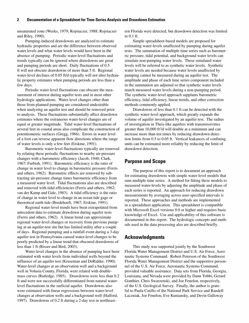
FiguresFigure 1. Daily precipitation, ground-water levels, barometric change, and earth tide at Air

Force Plant 6, Marietta, Georgia, April 22 to May 28, 2004. .................................................... 3Figure 2. Two time series with different collection frequencies and sampling times ........................ 5Figure 3. Example fitting period, April 17 to 30, 1997, and an estimation period, May 1 to 5, 1997. .. 5Figure 4. Barometric change, earth tide, and ground-water levels in wells TR-3 and SM-23-1

in the Amargosa Desert, Nevada, April 17 to May 1, 1997. .................................................... 6Figure 5. Improvement of synthetic water level for well SM-23-1, April 17 to May 1, 1997, by

sequentially analyzing barometric change, earth tide, and water levels in well TR-3. ..... 7Figure 6. Example of drawdown filter, sub-periods, and averaging periods. ...................................... 8Figure 7. Water levels in wells HYPO-1, HYPO-5, and modified TR-3 and drawdowns in

wells HYPO-1 and HYPO-5, April 26 to May 11, 1997. .............................................................. 9Figure 8. Water levels in well HYPO-5 and Theis, raw, and filtered drawdowns, April 26 to

May 11, 1997. ................................................................................................................................ 10Figure 9. Fitting and prediction error comparison sites. ....................................................................... 10Figure 10. Measured water levels, synthetic water levels, and water-level components in

well SM-23-1, Nevada, during a 14-day fitting period and a 7-day prediction period that began May 1, 1997. .............................................................................................................. 11

Figure 11. Fitting and prediction errors for five synthetic water levels in well sct4 in Georgia, with a 7-day prediction period that begins May 27, 2004. .................................................... 13

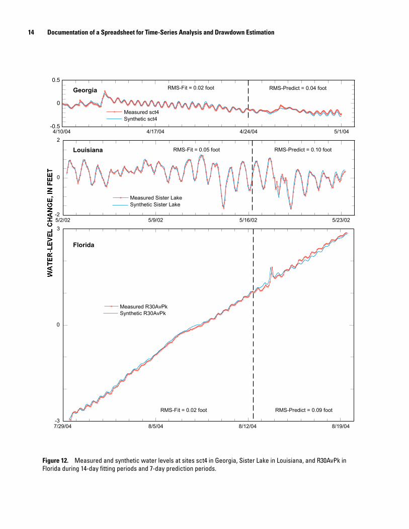
Figure 12. Measured and synthetic water levels at sites sct4 in Georgia, Sister Lake in Louisiana, and R30AvPk in Florida during 14-day fitting periods and 7-day prediction periods. ......................................................................................................................................... 14

Figure 13. Example of Excel forms for changing security settings. ...................................................... 15Figure 14. Example of TimeSeries page with data entered. ................................................................... 16

TablesTable 1. Sites with water-level time series that were used to create synthetic water levels ........ 8Table 2. Ratios of prediction-to-fitting errors, prediction periods, water-level ranges, and

prediction-error ranges at sites in Florida, Georgia, Louisiana, and Nevada .................. 12

Appendix Step-by-Step Instructions for Nevada Example .......................................................................................... 35

v

Conversion Factors and DatumsMultiply By To obtain

inch (in.) 25.4 millimeter (mm)

foot (ft) 0.3048 meter (m)

foot per day (ft/d) 0.3048 meter per day (m/d)

foot squared per day1 (ft2/d) 0.0929 meter squared per day (m2/d)

gallon per minute (gal/min) 0.06308 liter per second (L/sec)

mile (mi) 1.609 kilometer (km)

1Expresses transmissivity. An alternative way of expressing transmissivity is cubic foot per day per square foot times foot of aquifer thickness [(ft3/d)ft2] ft.

Horizontal coordinate information is referenced to the North American Datum of 1927 (NAD 27). Vertical coordinate information is referenced to the National Geodetic Vertical Datum of 1929 (NGVD 29). Altitude, as used in this report, refers to distance above the vertical datum.

vi

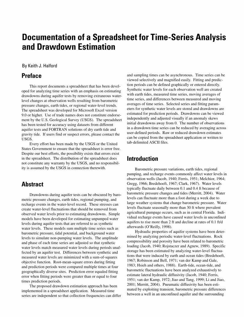
Preface This report documents a spreadsheet that has been devel-

oped for analyzing time series with an emphasis on estimating drawdowns during aquifer tests by removing extraneous water-level changes at observation wells resulting from barometric pressure changes, earth tides, or regional water-level trends. The spreadsheet was developed for Microsoft Excel version 9.0 or higher. Use of trade names does not constitute endorse-ment by the U.S. Geological Survey (USGS). The spreadsheet has been tested for accuracy using datasets from different aquifer tests and FORTRAN solutions of dry earth tide and gravity tide. If users find or suspect errors, please contact the USGS.

Every effort has been made by the USGS or the United States Government to ensure that the spreadsheet is error free. Despite our best efforts, the possibility exists that errors exist in the spreadsheet. The distribution of the spreadsheet does not constitute any warranty by the USGS, and no responsibil-ity is assumed by the USGS in connection therewith.

Abstract Drawdowns during aquifer tests can be obscured by baro-

metric pressure changes, earth tides, regional pumping, and recharge events in the water-level record. These stresses can create water-level fluctuations that should be removed from observed water levels prior to estimating drawdowns. Simple models have been developed for estimating unpumped water levels during aquifer tests that are referred to as synthetic water levels. These models sum multiple time series such as barometric pressure, tidal potential, and background water levels to simulate non-pumping water levels. The amplitude and phase of each time series are adjusted so that synthetic water levels match measured water levels during periods unaf-fected by an aquifer test. Differences between synthetic and measured water levels are minimized with a sum-of-squares objective function. Root-mean-square errors during fitting and prediction periods were compared multiple times at four geographically diverse sites. Prediction error equaled fitting error when fitting periods were greater than or equal to four times prediction periods.

The proposed drawdown estimation approach has been implemented in a spreadsheet application. Measured time series are independent so that collection frequencies can differ

and sampling times can be asynchronous. Time series can be viewed selectively and magnified easily. Fitting and predic-tion periods can be defined graphically or entered directly. Synthetic water levels for each observation well are created with earth tides, measured time series, moving averages of time series, and differences between measured and moving averages of time series. Selected series and fitting param-eters for synthetic water levels are stored and drawdowns are estimated for prediction periods. Drawdowns can be viewed independently and adjusted visually if an anomaly skews initial drawdowns away from 0. The number of observations in a drawdown time series can be reduced by averaging across user-defined periods. Raw or reduced drawdown estimates can be copied from the spreadsheet application or written to tab-delimited ASCII files.

IntroductionBarometric pressure variations, earth tides, regional

pumping, and recharge events commonly affect water levels in observation wells (Jacob, 1940; Ferris, 1951; Melchior, 1964; Gregg, 1966; Bredehoeft, 1967; Clark, 1967). Water levels typically fluctuate daily between 0.1 and 0.4 ft because of barometric pressure changes and tides (Merritt, 2004). Water levels can fluctuate more than a foot during a week due to large weather systems that change barometric pressure. Water levels fluctuate seasonally more than 30 ft where prevalent agricultural pumpage occurs, such as in central Florida. Indi-vidual recharge events have caused water levels in unconfined aquifers to rise more than 2 ft and decline at rates of 0.1 ft/d afterwards (O’Reilly, 1998).

Hydraulic properties of aquifer systems have been deter-mined by analyzing periodic water-level fluctuations. Rock compressibility and porosity have been related to barometric loading (Jacob, 1940; Rojstaczer and Agnew, 1989). Specific storage has been estimated by analyzing water-level fluctua-tions that were induced by earth and ocean tides (Bredehoeft, 1967; Robinson and Bell, 1971; van der Kamp and Gale, 1983; Hsieh and others, 1988). Earth-tide, ocean-tide, and barometric fluctuations have been analyzed exhaustively to estimate lateral hydraulic diffusivity (Jacob, 1940; Ferris, 1951; van der Kamp, 1972; Jiao and Tang, 1999; Li and Jiao, 2001; Merritt, 2004). Pneumatic diffusivity has been esti-mated by exploiting transient, barometric pressure differences between a well in an unconfined aquifer and the surrounding


By Keith J. Halford

unsaturated zone (Weeks, 1979; Rojstaczer, 1988; Rojstaczer and Riley, 1990).

Pumping-induced drawdowns are analyzed to estimate hydraulic properties and are the difference between observed water levels and what water levels would have been in the absence of pumping. Periodic water-level fluctuations and trends typically can be ignored where drawdowns are great and pumping periods are short. Daily fluctuations of 0.5 ft will not obscure drawdowns of more than 5 ft. Regional water-level declines of 0.05 ft/d typically will not alter hydrau-lic property estimates when pumping periods are less than a few days.

Periodic water-level fluctuations can obscure the mea-surement of interest during aquifer tests and in most other hydrologic applications. Water-level changes other than those from planned pumping are considered undesirable when analyzing an aquifer test and should be removed prior to analysis. These fluctuations substantially affect drawdown estimates where the extraneous water-level changes are of equal or greater magnitude. Tidal water-level fluctuations of several feet in coastal areas also complicate the construction of potentiometric surfaces (Gregg, 1966). Errors in water level of a foot can reverse apparent flow directions where the range of water levels is only a few feet (Erskine, 1991).

Barometric water-level fluctuations typically are removed by relating these periodic fluctuations to nearby air-pressure changes with a barometric efficiency (Jacob, 1940; Clark, 1967; Furbish, 1991). Barometric efficiency is the ratio of change in water level to change in barometric pressure (Ferris and others, 1962). Barometric effects are removed by sub-tracting air-pressure change times barometric efficiency from a measured water level. Tidal fluctuations also are described and removed with tidal efficiencies (Ferris and others, 1962; van der Kamp and Gale, 1983). A tidal efficiency is the ratio of change in water level to change in an ocean tide gage or theoretical earth tide (Bredehoeft, 1967; Erskine, 1991).

Regional water-level trends have been extrapolated from antecedent data to estimate drawdown during aquifer tests (Ferris and others, 1962). A linear trend can approximate regional water-level changes or recovery from previous pump-ing at an aquifer-test site but has limited utility after a couple of days. Regional pumping and a rainfall event during a 3-day aquifer test in Pennsylvania caused water-level changes to be poorly predicted by a linear trend that obscured drawdowns of less than 1 ft (Risser and Bird, 2003).

Water-level changes in the absence of pumping have been estimated with water levels from individual wells beyond the influence of an aquifer test (Kruseman and DeRidder, 1990). Water-level changes at an observation well and a background well in Volusia County, Florida, were related with double-mass curves (Rutledge, 1985). Drawdowns were less than 0.2 ft and were not successfully differentiated from natural water-level fluctuations in the surficial aquifer. Drawdowns also were estimated with linear regressions between water-level changes at observation wells and a background well (Halford, 1997). Drawdowns of 0.2 ft during a 2-day test in northeast-

ern Florida were detected, but drawdown detection was limited to 0.1 ft.

Simple spreadsheet-based models are proposed for estimating water-levels unaffected by pumping during aquifer tests. The summation of multiple time series such as baromet-ric pressure, tidal potential, and background water levels can simulate non-pumping water levels. These simulated water levels will be referred to as synthetic water levels. Synthetic water levels are needed because water levels unaffected by pumping cannot be measured during an aquifer test. The amplitude and phase of each time series component included in the summation are adjusted so that synthetic water levels match measured water levels during a non-pumping period. The synthetic water-level approach supplants barometric efficiency, tidal efficiency, linear trends, and other correction methods commonly applied.

Drawdowns of less than 0.1 ft can be detected with the synthetic water-level approach, which greatly expands the volume of aquifer investigated by an aquifer test. The radius of investigation in Theis-like aquifers with transmissivities greater than 10,000 ft2/d will double at a minimum and can increase more than ten times by reducing drawdown detec-tion limits from 0.5 to 0.05 ft. Vertical leakances of confining units can be estimated more reliably by reducing the limit of drawdown detection.

Purpose and Scope

The purpose of this report is to document an approach for estimating drawdowns with simple water-level models that sum multiple time series. A method for fitting these models to measured water-levels by adjusting the amplitude and phase of each series is reported. An approach for reducing drawdown measurements by averaging across user-specified intervals is reported. These approaches and methods are implemented in a spreadsheet application. This spreadsheet is compatible with Microsoft Excel versions 9.0 or higher and requires basic knowledge of Excel. Use and applicability of this software is documented in this report. The hydrologic concepts and meth-ods used in the data processing also are described briefly.

Acknowledgments

This study was supported jointly by the Southwest Florida Water Management District and U.S. Air Force, Aero-nautic Systems Command. Robert Peterson of the Southwest Florida Water Management District and the supportive person-nel of the U.S. Air Force, Aeronautic Systems Command, provided valuable assistance. Data sets from Florida, Georgia, Louisiana, and Nevada were provided by Dann Yobbi, Gerard Gonthier, Chris Swarzenski, and Joe Fenelon, respectively, of the U.S. Geological Survey. Finally, the author is grate-ful to Paula Cutillo of the National Park Service and Randell Laczniak, Joe Fenelon, Eve Kuniansky, and Devin Galloway

2 Documentation of a Spreadsheet for Time-Series Analysis and Drawdown Estimation

of the U.S. Geological Survey for materially improving the drawdown-estimation spreadsheet and report.

Water-Level ComponentsBarometric pressure, tidal potential, background water

levels, stream stage, and any other time series are potential components in a water-level record. The relevant components can be selected where a relation in the water-level record is expected. For example, a relation between barometric pres-sure and water levels in well sct4 is not obvious (fig. 1), but a relation is expected. A barometric pressure component should be included to test if barometric pressure improves a synthetic water-level series of well sct4.

Barometric Effects

Barometric changes cause greater water-level fluctuations in deeper, confined aquifers where rock matrix absorbs more of the atmospheric load (Merritt, 2004). Fluctuations increase because pressure instantly affects water levels in wells while a stiffer rock matrix transfers little of the increased atmospheric load to the confined water column. Atmospherically induced water-level fluctuations typically are less than 0.2 ft during a day. Large barometric pressure changes from regional storms can cause water-level fluctuations of about 1 ft during a week.

Barometric changes also measurably affect water levels in unconfined aquifers (Weeks, 1979). Pressure changes do not propagate instantaneously through the unsaturated zone because air is highly compressible. The relatively low pneu-matic diffusivity of the unsaturated zone creates substantial lags between atmospheric and water-level changes. Uncon-

0

1

2

3

4/22 4/29 5/6 5/13 5/20 5/272004

b4mwhrw204sct4BarometerEarth tide

0

1

2

WA

TE

R-L

EV

EL

CH

AN

GE

, IN

FE

ET

DA

ILY

PR

EC

IPIT

AT

ION

,IN

INC

HE

S

Figure 1. Daily precipitation, ground-water levels, barometric change, and earth tide at Air Force Plant 6, Mari-etta, Georgia, April 22 to May 28, 2004.

Water-Level Components �

fined water-level fluctuations can approach the magnitude of confined water-level fluctuations as the depth to water exceeds 500 ft.

Tidal Effects

Tides result from changes in gravitational forces as the relative positions of sun, moon, and earth change. The diurnal rise and fall of ocean levels are the most common manifes-tation of varying gravitational forces and are referred to as ocean tides. Ocean tides affect ground-water levels through direct head changes in an aquifer or as loads applied through a confining unit (Merritt, 2004). Ocean tide effects are better approximated with a nearby tidal gage that also incorporates wind and coastal geometry effects in addition to direct gravita-tional forcing.

Tidal forces also distort the crust of the earth which cre-ates water-level fluctuations in mid-continent wells (Brede-hoeft, 1967; Marine, 1975; Hanson and Owen, 1982; Narasim-han and others, 1984). Earth tides periodically deform (dilate and compress) the skeleton of the aquifer system, changing the porosity and causing measurable water-level fluctuations of as much as 0.1 ft or more in wells penetrating aquifers with small storage coefficients (fig. 1). Coupling between the mechanical deformation and the fluid filling the secondary porosity ampli-fies water-level response in wells hydraulically connected to the secondary-porosity features. The presence of secondary porosity typically renders the formation more compliant to imposed stresses depending on orientation of the fractures or faults with respect to the principal component directions of the imposed stress. The theoretical crustal strain tensors resulting from the two principal lunar daily and semidiurnal tides (O

1

and M2) are largely horizontal and orthogonal to one another.

Subvertical fractures with azimuths oriented perpendicular to the strain tensor for a particular tide tend to amplify the strain and thereby the water-level response (Bower, 1983).

Two theoretical earth tides are included as internal func-tions in the drawdown estimation spreadsheet. The first earth tide function computes the areal strain tide in parts per billion (ppb), and the second function computes the gravity tide in microgals (µgal) downward normal to the Earth ellipsoid (Har-rison, 1971).

Background Water Levels

Recharge events and regional pumping are identifiable stresses that typically affect large areas but are not predicted easily with independent time series such as barometric change and tidal potential. Recharge events and regional pump-ing stresses create similar water-level changes in multiple wells over areas of many square miles. Water levels in wells sufficiently removed from an aquifer test can simulate these regional stresses and any other unidentified stresses. Water levels in these remote wells will be referred to as background water levels.

Background water levels can be more effective correctors than independent barometric and tidal time series even where only barometric and tidal stresses are significant. Barometric forcing through the unsaturated zone lags behind because of the low permeability of unsaturated rock relative to an open well (Weeks, 1979). The complex relation between baromet-ric pressure and water levels in a well are explained poorly with a barometric efficiency where the unsaturated zone is thick. Background water levels from another well of similar construction better approximate this relation. Likewise, rock properties and fracture orientation in an aquifer control tidal water-level fluctuations as much as dry earth tide. Water levels from background wells can better approximate the rock-tide interaction than just dry earth tide.

Moving Averages and Differences

Amplitudes of diurnal water-level fluctuations in wells frequently differ from lower frequency changes such as frontal barometric changes. Frequency dependent differences in water-level fluctuations exist between wells because of dif-ferences in well construction and aquifer properties. Diurnal water-level fluctuations will be less where communication between well and aquifer is impeded and wellbore storage is increased. Poorly developed wells with large casing diameters and short screens damp high frequency water-level fluctua-tions. Low transmissivity aquifers with large storage coeffi-cients also will damp water-level fluctuations.

Low frequency signals are separated from diurnal water-level fluctuations with moving averages of the original time series in the spreadsheet. Water levels typically are averaged over 12-hour or 24-hour periods, but any averaging periods can be specified. High frequency signals are differences between the raw time series and the moving averages. Three time series: raw, moving average, and differences, are avail-able for each water-level series.

Drawdown Estimation with Synthetic Water Levels

Drawdowns are differences between measured and syn-thetic water levels that are created for each observation well. Multiple time series such as barometric change, earth tide, and background water levels are specified as components of a syn-thetic water-level series. Synthetic water levels are modified by adjusting the amplitude and phase of each component. The synthetic water level at time, t, is

∑=

++−+=n

iiii tVattCCtSWL

1010 )()()( φ

(1)

where:


0C isanoffset,L, 1C istheslopeofwater-levelchange,inLT-1, n isthenumberoftime-seriescomponents, ia istheamplitudemultiplieroftheithcomponent,

inL(unitsofithcomponent)-1, iφ isthephase-shiftoftheithcomponent,T,and )( ii tV φ+ isthevalueoftheithcomponentattime it φ+

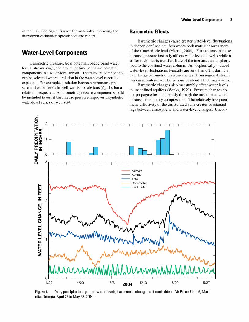
inunitsofithcomponent.Each time series, iV , is a smooth function because values

are interpolated between consecutive data pairs. Interpola-tion allows data to be collected at variable intervals within a time series. This also means collection frequencies can differ between time series and do not need to be synchronized (fig. 2).

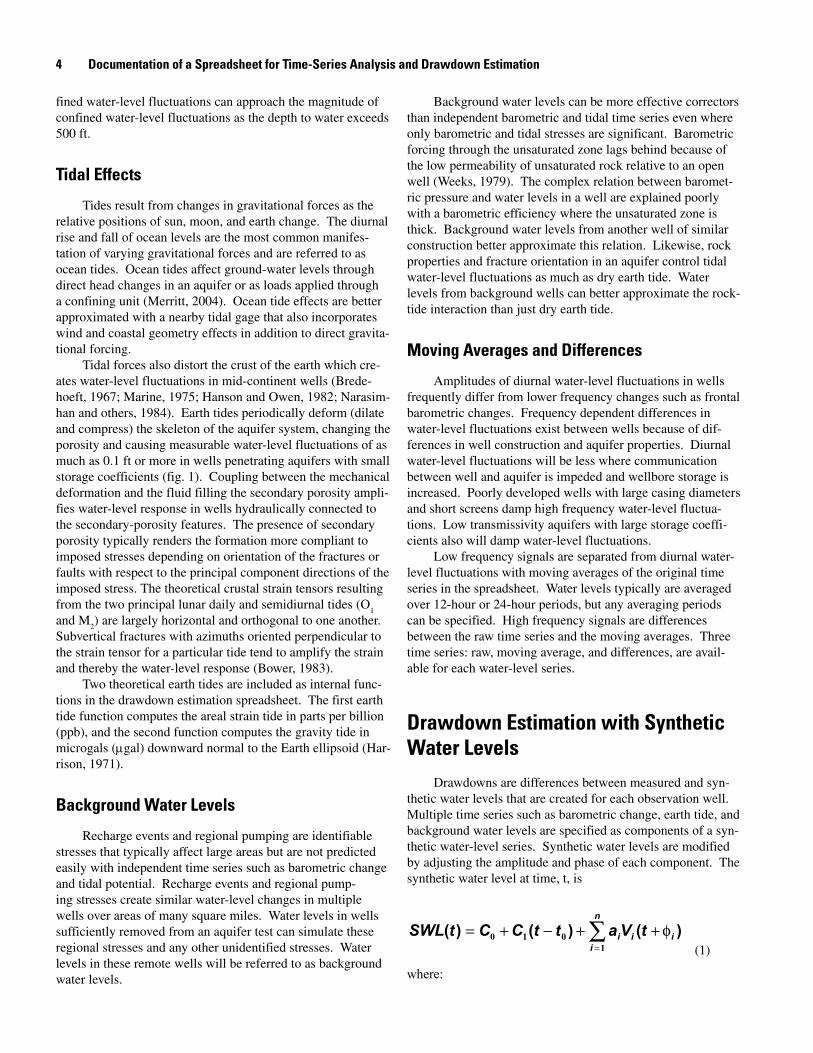
The amplitude and phase of each component are adjusted so synthetic water levels match measured water levels during

periods unaffected by an aquifer test. These periods will be referred to as fitting periods. A sum-of-squares of differences between synthetic and measured water levels is minimized to estimate amplitudes and phases. Root-mean-square (RMS) error is reported instead of sum-of-squares so error and the range of fluctuation can be compared easily.

Amplitude and phase estimates typically are non-unique, which is not important for drawdown estimation. Synthetic water levels are the important result, not parameter estimates. Amplitude estimates remain unique until two or more of the components are highly correlated. Phase estimates are non-unique regardless of the number of components because many local minima exist. Adjustment of the phase of each compo-nent is limited to a user-defined range. Sensitivity should be tested with multiple initial phase estimates because synthetic water-level estimates frequently can be improved.

Fitting periods should coincide with non-testing condi-tions where all stresses other than pumping for an aquifer test affect water levels. Ideally, a fitting period will be immedi-ately antecedent to an aquifer test. Differences between an antecedent fitting period and an estimation period are com-pared easily because water-level changes are greatest at the beginning of an aquifer test (fig. 3). A fitting period can occur after an aquifer test, but synthetic water-level will not simulate measured water levels as well if water levels are still recover-ing or background conditions have changed.

Components of the synthetic water-level record are selected by trial-and-error. Time series that mimic the water-level record to be analyzed should be selected (fig. 4). Back-ground water levels frequently best approximate the water levels to be analyzed. Irrelevant components make the fitting process take longer but do not degrade the predictive capac-ity of synthetic water levels. The amplitude of an irrelevant component will approach zero, which causes this component to negligibly affect the synthetic water levels.

WA

TE

R-L

EV

EL

CH

AN

GE

, IN

FE

ET

TIME, IN HOUR:MINUTE

Series 1Series 2

0

0.05

0.10

0:00 6:00 12:00

Figure 2. Two time series with different collection fre-quencies and sampling times.

-0.6

-0.3

0

0.3

0.6

4/20 4/25 4/30 5/5 5/10 5/151997

Fitting period Estimation period

Measured

Synthetic

Differences

Figure �. Example fitting period, April 17 to 30, 1997, and an estimation period, May 1 to 5, 1997.

Drawdown Estimation with Synthetic Water Levels 5

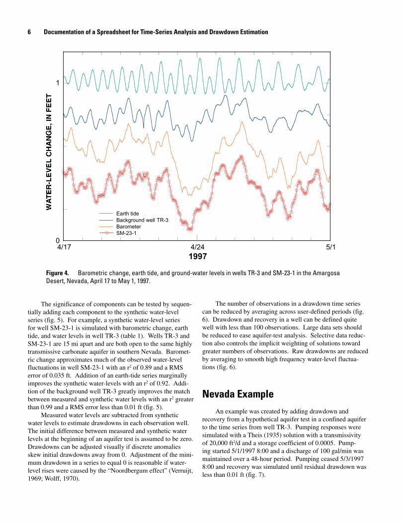
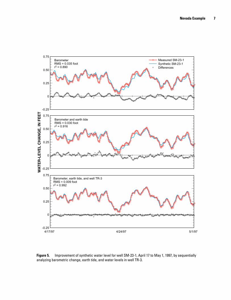
The significance of components can be tested by sequen-tially adding each component to the synthetic water-level series (fig. 5). For example, a synthetic water-level series for well SM-23-1 is simulated with barometric change, earth tide, and water levels in well TR-3 (table 1). Wells TR-3 and SM-23-1 are 15 mi apart and are both open to the same highly transmissive carbonate aquifer in southern Nevada. Baromet-ric change approximates much of the observed water-level fluctuations in well SM-23-1 with an r2 of 0.89 and a RMS error of 0.035 ft. Addition of an earth-tide series marginally improves the synthetic water-levels with an r2 of 0.92. Addi-tion of the background well TR-3 greatly improves the match between measured and synthetic water levels with an r2 greater than 0.99 and a RMS error less than 0.01 ft (fig. 5).

Measured water levels are subtracted from synthetic water levels to estimate drawdowns in each observation well. The initial difference between measured and synthetic water levels at the beginning of an aquifer test is assumed to be zero. Drawdowns can be adjusted visually if discrete anomalies skew initial drawdowns away from 0. Adjustment of the mini-mum drawdown in a series to equal 0 is reasonable if water-level rises were caused by the “Noordbergum effect” (Verruijt, 1969; Wolff, 1970).

The number of observations in a drawdown time series can be reduced by averaging across user-defined periods (fig. 6). Drawdown and recovery in a well can be defined quite well with less than 100 observations. Large data sets should be reduced to ease aquifer-test analysis. Selective data reduc-tion also controls the implicit weighting of solutions toward greater numbers of observations. Raw drawdowns are reduced by averaging to smooth high frequency water-level fluctua-tions (fig. 6).

Nevada Example An example was created by adding drawdown and

recovery from a hypothetical aquifer test in a confined aquifer to the time series from well TR-3. Pumping responses were simulated with a Theis (1935) solution with a transmissivity of 20,000 ft2/d and a storage coefficient of 0.0005. Pump-ing started 5/1/1997 8:00 and a discharge of 100 gal/min was maintained over a 48-hour period. Pumping ceased 5/3/1997 8:00 and recovery was simulated until residual drawdown was less than 0.01 ft (fig. 7).

0

1

4/17 4/24 5/1

1997

Earth tide

Background well TR-3

Barometer

SM-23-1

Figure 4. Barometric change, earth tide, and ground-water levels in wells TR-3 and SM-23-1 in the Amargosa Desert, Nevada, April 17 to May 1, 1997.


BarometerRMS = 0.035 footr2 = 0.890

WA

TE

R-L

EV

EL

CH

AN

GE

, IN

FE

ET

Barometer and earth tideRMS = 0.030 footr2 = 0.916

Barometer, earth tide, and well TR-3RMS = 0.009 footr2 = 0.992

Measured SM-23-1Synthetic SM-23-1Differences

-0.25

0

0.25

0.50

0.75

-0.25

0

0.25

0.50

0.75

-0.25

0

0.25

0.50

0.75

4/17/97 4/24/97 5/1/97

Figure 5. Improvement of synthetic water level for well SM-23-1, April 17 to May 1, 1997, by sequentially analyzing barometric change, earth tide, and water levels in well TR-3.

Nevada Example �

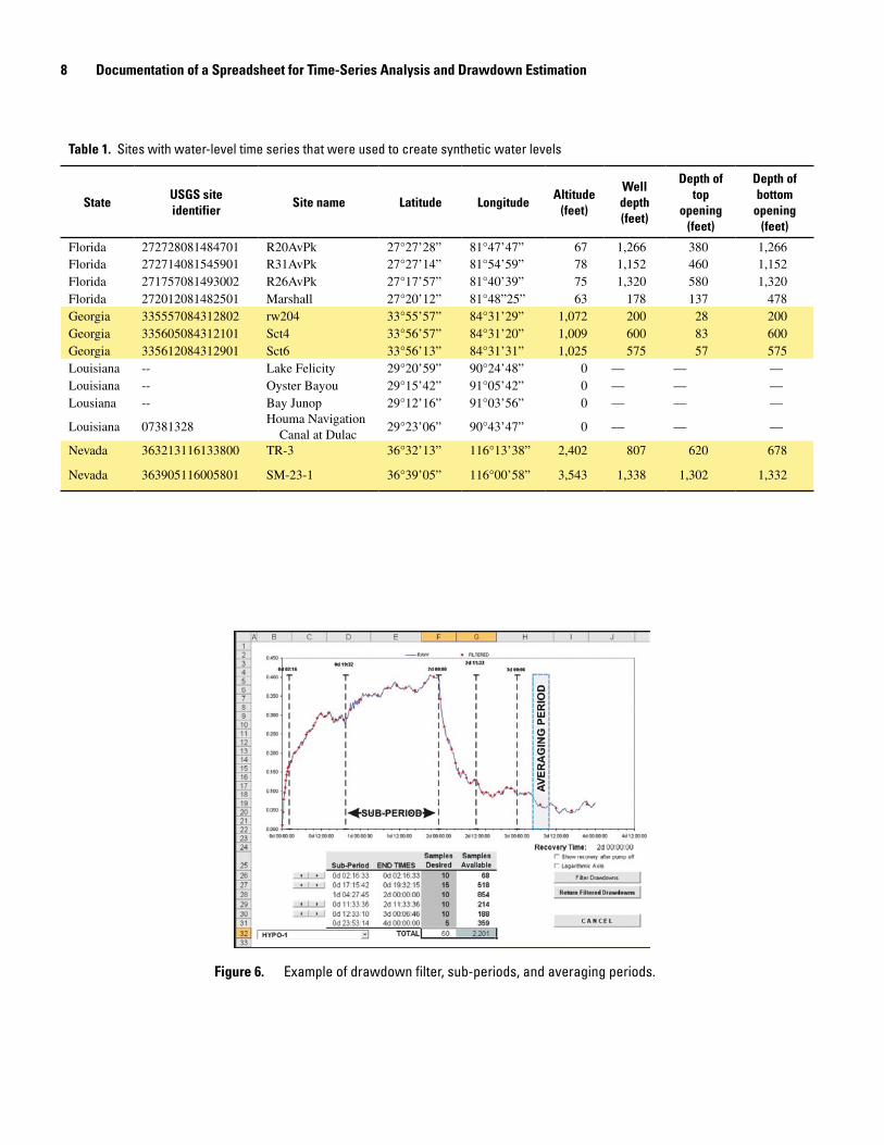
Figure 6. Example of drawdown filter, sub-periods, and averaging periods.

� Documentation of a Spreadsheet for Time-Series Analysis and Drawdown Estimation

Table 1. Sites with water-level time series that were used to create synthetic water levels

StateUSGS site identifier

Site name Latitude LongitudeAltitude

(feet)

Well depth (feet)

Depth of top

opening (feet)

Depth of bottom

opening (feet)

Florida 272728081484701 R20AvPk 27°27’28” 81°47’47” 67 1,266 380 1,266Florida 272714081545901 R31AvPk 27°27’14” 81°54’59” 78 1,152 460 1,152Florida 271757081493002 R26AvPk 27°17’57” 81°40’39” 75 1,320 580 1,320Florida 272012081482501 Marshall 27°20’12” 81°48”25” 63 178 137 478Georgia 335557084312802 rw204 33°55’57” 84°31’29” 1,072 200 28 200Georgia 335605084312101 Sct4 33°56’57” 84°31’20” 1,009 600 83 600Georgia 335612084312901 Sct6 33°56’13” 84°31’31” 1,025 575 57 575Louisiana -- Lake Felicity 29°20’59” 90°24’48” 0 — — —Louisiana -- Oyster Bayou 29°15’42” 91°05’42” 0 — — —Lousiana -- Bay Junop 29°12’16” 91°03’56” 0 — — —

Louisiana 07381328Houma Navigation

Canal at Dulac29°23’06” 90°43’47” 0 — — —

Nevada 363213116133800 TR-3 36°32’13” 116°13’38” 2,402 807 620 678

Nevada 363905116005801 SM-23-1 36°39’05” 116°00’58” 3,543 1,338 1,302 1,332

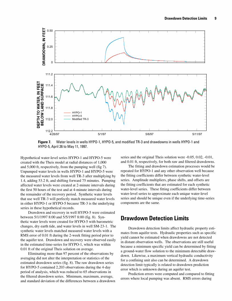
Hypothetical water-level series HYPO-1 and HYPO-5 were created with the Theis model at radial distances of 1,000 and 5,000 ft, respectively, from the pumping well (fig 7). Unpumped water levels in wells HYPO-1 and HYPO-5 were the measured water levels from well TR-3 after multiplying by 1.4, adding 53.2 ft, and shifting forward 75 minutes. Pumping affected water levels were created at 2-minute intervals during the first 50 hours of the test and at 4-minute intervals during the remainder of the recovery period. Synthetic water levels that use well TR-3 will perfectly match measured water levels in either HYPO-1 or HYPO-5 because TR-3 is the underlying series in these hypothetical records.

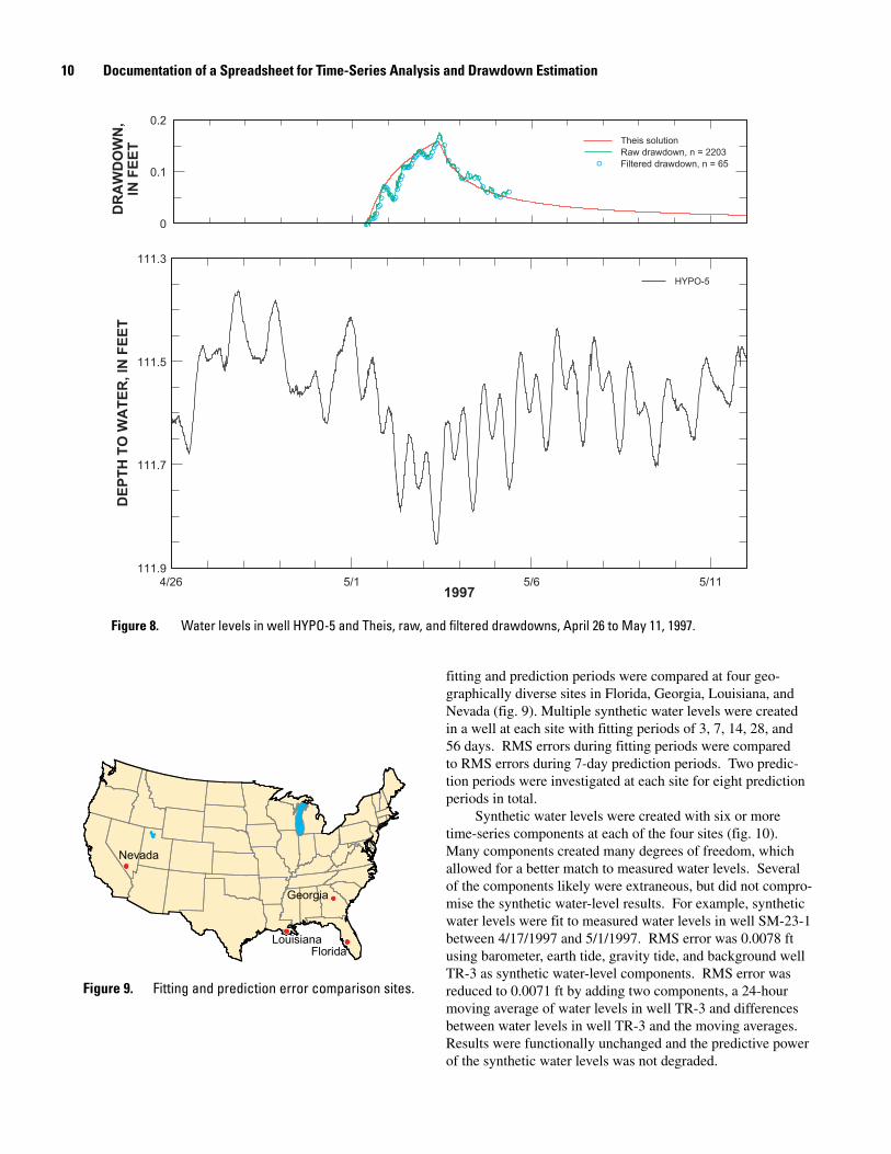
Drawdown and recovery in well HYPO-5 were estimated between 5/1/1997 8:00 and 5/5/1997 8:00 (fig. 8). Syn-thetic water levels were created for HYPO-5 with barometric changes, dry earth tide, and water levels in well SM-23-1. The synthetic water levels matched measured water levels with a RMS error of 0.01 ft during the 2-week fitting period prior to the aquifer test. Drawdown and recovery were observed easily in the estimated time-series for HYPO-1, which was within 0.01 ft of the original Theis solution on average.

Eliminating more than 97 percent of the observations by averaging did not alter the interpretation or statistics of the estimated drawdown series (fig. 8). The raw drawdown series for HYPO-5 contained 2,203 observations during the 4-day period of analysis, which was reduced to 65 observations in the filtered drawdown series. Minimum, maximum, average, and standard deviation of the differences between a drawdown

series and the original Theis solution were -0.05, 0.02, -0.01, and 0.01 ft, respectively, for both raw and filtered drawdowns.

The fitting and drawdown estimation processes would be repeated for HYPO-1 and any other observation well because the fitting coefficients differ between synthetic water-level series. Amplitude multipliers, phase shifts, and offsets are the fitting coefficients that are estimated for each synthetic water-level series. These fitting coefficients differ between water-level series to approximate each unique water-level series and should be unique even if the underlying time-series components are the same.

Drawdown Detection LimitsDrawdown detection limits affect hydraulic property esti-

mates from aquifer tests. Hydraulic properties such as specific yield cannot be estimated when drawdowns are not detected in distant observation wells. The observations are still useful because a minimum specific yield can be determined by fitting a ground-water flow solution to the minimum detectable draw-down. Likewise, a maximum vertical hydraulic conductivity for a confining unit also can be determined. A drawdown detection limit typically is related to drawdown prediction error which is unknown during an aquifer test.

Prediction errors were computed and compared to fitting errors where local pumping was absent. RMS errors during

4/26/97 5/1/97 5/6/97

0

0.25

0.50

HYPO-1

HYPO-5

Modified TR-3

5/11/97

112.2

112.0

111.8

111.6

111.4

111.2

Figure �. Water levels in wells HYPO-1, HYPO-5, and modified TR-3 and drawdowns in wells HYPO-1 and HYPO-5, April 26 to May 11, 1997.

Drawdown Detection Limits �

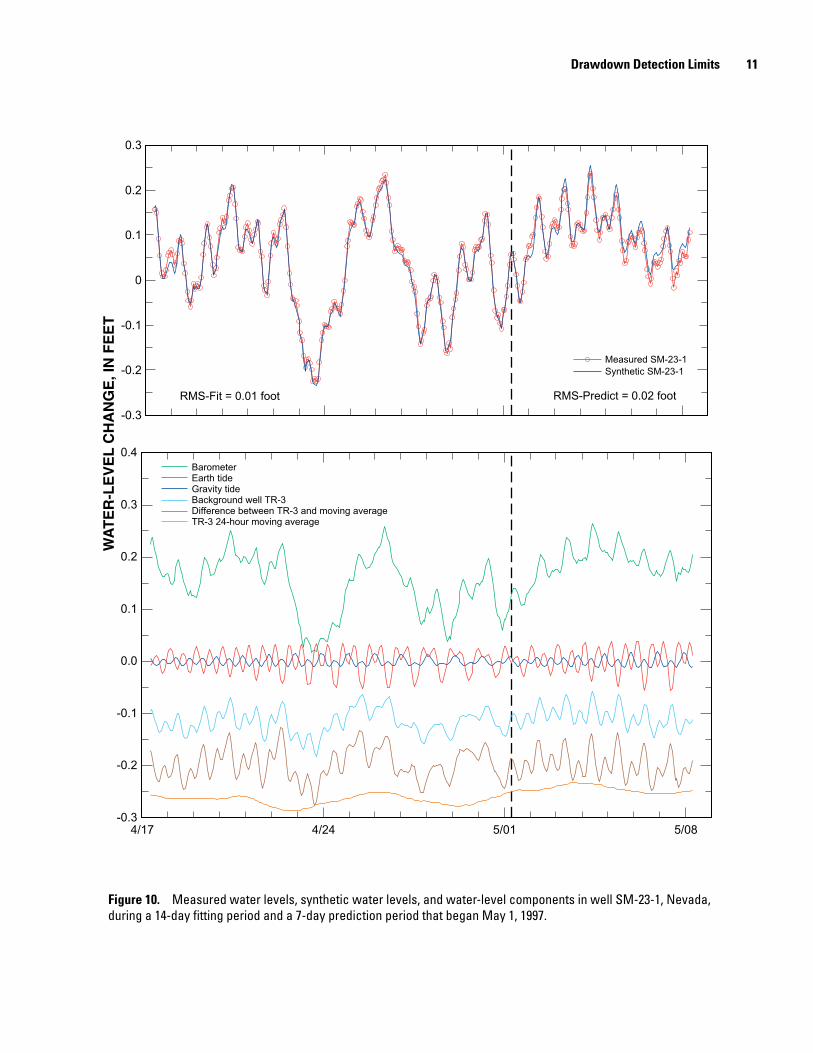
fitting and prediction periods were compared at four geo-graphically diverse sites in Florida, Georgia, Louisiana, and Nevada (fig. 9). Multiple synthetic water levels were created in a well at each site with fitting periods of 3, 7, 14, 28, and 56 days. RMS errors during fitting periods were compared to RMS errors during 7-day prediction periods. Two predic-tion periods were investigated at each site for eight prediction periods in total.

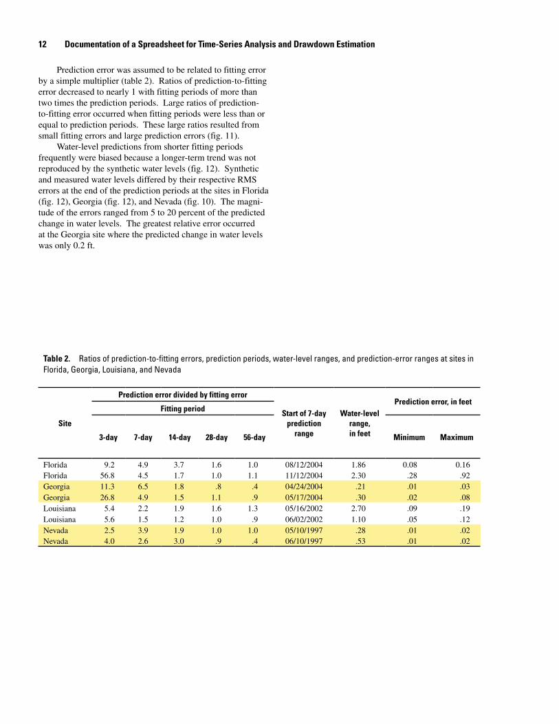
Synthetic water levels were created with six or more time-series components at each of the four sites (fig. 10). Many components created many degrees of freedom, which allowed for a better match to measured water levels. Several of the components likely were extraneous, but did not compro-mise the synthetic water-level results. For example, synthetic water levels were fit to measured water levels in well SM-23-1 between 4/17/1997 and 5/1/1997. RMS error was 0.0078 ft using barometer, earth tide, gravity tide, and background well TR-3 as synthetic water-level components. RMS error was reduced to 0.0071 ft by adding two components, a 24-hour moving average of water levels in well TR-3 and differences between water levels in well TR-3 and the moving averages. Results were functionally unchanged and the predictive power of the synthetic water levels was not degraded.

5/1 5/6 5/111997

DE

PT

H T

O W

AT

ER

, IN

FE

ET

4/26111.9

111.7

111.5

111.3

DR

AW

DO

WN

,IN

FE

ET

0

0.1

0.2

HYPO-5

Theis solutionRaw drawdown, n = 2203Filtered drawdown, n = 65

Figure �. Water levels in well HYPO-5 and Theis, raw, and filtered drawdowns, April 26 to May 11, 1997.

Nevada

FloridaLouisiana

Georgia

Figure �. Fitting and prediction error comparison sites.


BarometerEarth tideGravity tideBackground well TR-3Difference between TR-3 and moving averageTR-3 24-hour moving average

-0.3

-0.3

-0.2

-0.1

0.0

0.1

0.2

0.3

0.4

4/17 4/24 5/01 5/08

-0.2

-0.1

0

0.1

0.2

0.3

RMS-Fit = 0.01 foot

Measured SM-23-1Synthetic SM-23-1

RMS-Predict = 0.02 foot

WA

TE

R-L

EV

EL

CH

AN

GE

, IN

FE

ET

Figure 10. Measured water levels, synthetic water levels, and water-level components in well SM-23-1, Nevada, during a 14-day fitting period and a 7-day prediction period that began May 1, 1997.

Drawdown Detection Limits 11

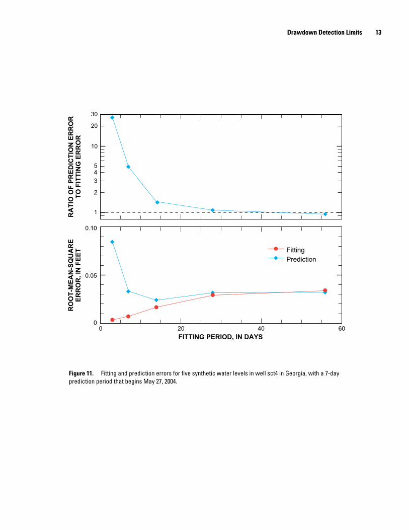
Prediction error was assumed to be related to fitting error by a simple multiplier (table 2). Ratios of prediction-to-fitting error decreased to nearly 1 with fitting periods of more than two times the prediction periods. Large ratios of prediction-to-fitting error occurred when fitting periods were less than or equal to prediction periods. These large ratios resulted from small fitting errors and large prediction errors (fig. 11).

Water-level predictions from shorter fitting periods frequently were biased because a longer-term trend was not reproduced by the synthetic water levels (fig. 12). Synthetic and measured water levels differed by their respective RMS errors at the end of the prediction periods at the sites in Florida (fig. 12), Georgia (fig. 12), and Nevada (fig. 10). The magni-tude of the errors ranged from 5 to 20 percent of the predicted change in water levels. The greatest relative error occurred at the Georgia site where the predicted change in water levels was only 0.2 ft.


Table 2. Ratios of prediction-to-fitting errors, prediction periods, water-level ranges, and prediction-error ranges at sites in Florida, Georgia, Louisiana, and Nevada

Site

Prediction error divided by fitting error

Start of �-day prediction

range

Water-level range, in feet

Prediction error, in feetFitting period

�-day �-day 14-day 2�-day 56-day Minimum Maximum

Florida 9.2 4.9 3.7 1.6 1.0 08/12/2004 1.86 0.08 0.16Florida 56.8 4.5 1.7 1.0 1.1 11/12/2004 2.30 .28 .92Georgia 11.3 6.5 1.8 .8 .4 04/24/2004 .21 .01 .03Georgia 26.8 4.9 1.5 1.1 .9 05/17/2004 .30 .02 .08Louisiana 5.4 2.2 1.9 1.6 1.3 05/16/2002 2.70 .09 .19Louisiana 5.6 1.5 1.2 1.0 .9 06/02/2002 1.10 .05 .12Nevada 2.5 3.9 1.9 1.0 1.0 05/10/1997 .28 .01 .02Nevada 4.0 2.6 3.0 .9 .4 06/10/1997 .53 .01 .02

0 20 40 600

0.05

0.10

RA

TIO

OF

PR

ED

ICT

ION

ER

RO

RT

O F

ITT

ING

ER

RO

RR

OO

T-M

EA

N-S

QU

AR

EE

RR

OR

, IN

FE

ET

1

2

5

34

10

20

30

FittingPrediction

FITTING PERIOD, IN DAYS

Figure 11. Fitting and prediction errors for five synthetic water levels in well sct4 in Georgia, with a 7-day prediction period that begins May 27, 2004.

Drawdown Detection Limits 1�

-0.5

0

0.5

4/10/04 4/17/04 4/24/04 5/1/04

Measured sct4

Synthetic sct4

-3

0

3

7/29/04 8/5/04 8/12/04 8/19/04

Measured R30AvPk

Synthetic R30AvPk

-2

0

2

5/2/02 5/9/02 5/16/02 5/23/02

Measured Sister Lake

Synthetic Sister Lake

RMS-Fit = 0.02 foot RMS-Predict = 0.04 footGeorgia

Louisiana

Florida

RMS-Fit = 0.05 foot RMS-Predict = 0.10 foot

RMS-Fit = 0.02 foot RMS-Predict = 0.09 foot

Figure 12. Measured and synthetic water levels at sites sct4 in Georgia, Sister Lake in Louisiana, and R30AvPk in Florida during 14-day fitting periods and 7-day prediction periods.


Instructions for Time-Series Analysis WorkbookTime-series analysis, data filtering, synthetic water-level simulation, and drawdown estimation are performed within an

Excel workbook, TimeSeries+Drawdown.RV1.0.xls. Workbook pages are revealed sequentially as needed to analyze time series. All four workbook pages remain visible after being used unless the “RESET ALL” button on the TimeSeries page is pressed. Pressing the “RESET ALL” button eliminates all user-defined data, removes all series from charts, and hides all worksheets but the TimeSeries page.

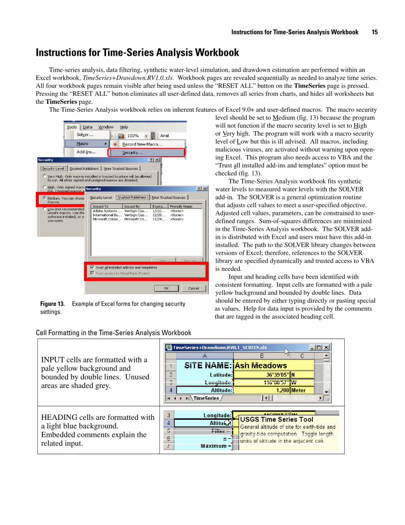
The Time-Series Analysis workbook relies on inherent features of Excel 9.0+ and user-defined macros. The macro security level should be set to Medium (fig. 13) because the program will not function if the macro security level is set to High or Very high. The program will work with a macro security level of Low but this is ill advised. All macros, including malicious viruses, are activated without warning upon open-ing Excel. This program also needs access to VBA and the “Trust all installed add-ins and templates” option must be checked (fig. 13).

The Time-Series Analysis workbook fits synthetic water levels to measured water levels with the SOLVER add-in. The SOLVER is a general optimization routine that adjusts cell values to meet a user-specified objective. Adjusted cell values, parameters, can be constrained to user-defined ranges. Sum-of-squares differences are minimized in the Time-Series Analysis workbook. The SOLVER add-in is distributed with Excel and users must have this add-in installed. The path to the SOLVER library changes between versions of Excel; therefore, references to the SOLVER library are specified dynamically and trusted access to VBA is needed.

Input and heading cells have been identified with consistent formatting. Input cells are formatted with a pale yellow background and bounded by double lines. Data should be entered by either typing directly or pasting special as values. Help for data input is provided by the comments that are tagged in the associated heading cell.

Cell Formatting in the Time-Series Analysis Workbook

INPUT cells are formatted with apale yellow background andbounded by double lines. Unusedareas are shaded grey.

HEADING cells are formatted witha light blue background.Embedded comments explain therelated input.

Figure 1�. Example of Excel forms for changing security settings.

Instructions for Time-Series Analysis Workbook 15

Step-by-Step InstructionsStep-by-step instructions for the TimeSeries+Drawdown spreadsheet also are provided in the appendix. The step-by-step

instructions explicitly track each operation used to analyze the Nevada example. Users are referred specifically to a workbook, page, and cell for each operation. Limited descriptions of the actions are reported.

TimeSeries Page

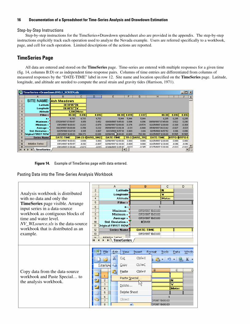
All data are entered and stored on the TimeSeries page. Time-series are entered with multiple responses for a given time (fig. 14, columns B:D) or as independent time-response pairs. Columns of time entries are differentiated from columns of measured responses by the “DATE-TIME” label in row 12. Site name and location specified on the TimeSeries page. Latitude, longitude, and altitude are needed to compute the areal strain and gravity tides (Harrison, 1971).

Figure 14. Example of TimeSeries page with data entered.

Analysis workbook is distributedwith no data and only theTimeSeries page visible. Arrangeinput series in a data-sourceworkbook as contiguous blocks oftime and water level.NV_WLsource.xls is the data-sourceworkbook that is distributed as anexample.

Copy data from the data-sourceworkbook and Paste Special… tothe analysis workbook.


Pasting Data into the Time-Series Analysis Workbook

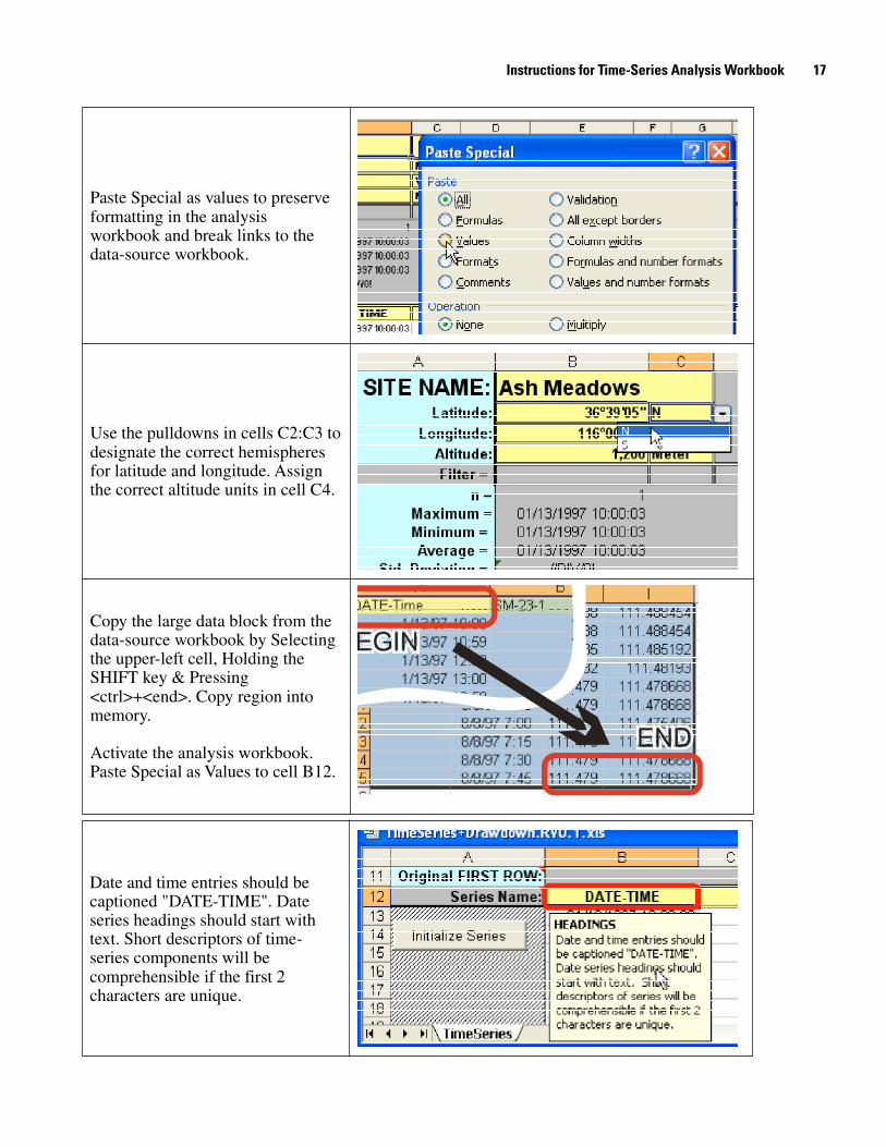
Paste Special as values to preserveformatting in the analysisworkbook and break links to thedata-source workbook.

Use the pulldowns in cells C2:C3 todesignate the correct hemispheresfor latitude and longitude. Assignthe correct altitude units in cell C4.

Copy the large data block from thedata-source workbook by Selectingthe upper-left cell, Holding theSHIFT key & Pressing<ctrl>+<end>. Copy region intomemory.

Activate the analysis workbook.Paste Special as Values to cell B12.

Date and time entries should becaptioned "DATE-TIME". Dateseries headings should start withtext. Short descriptors of time-series components will becomprehensible if the first 2characters are unique.

Instructions for Time-Series Analysis Workbook 1�

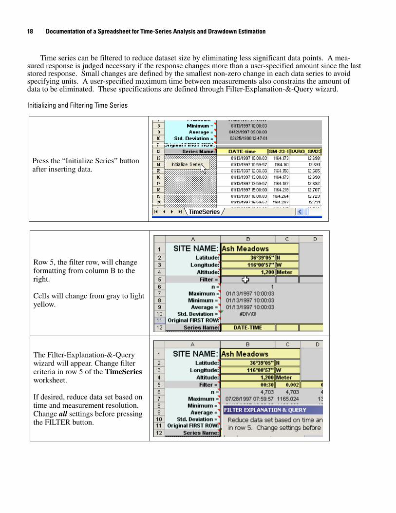
Time series can be filtered to reduce dataset size by eliminating less significant data points. A mea-sured response is judged necessary if the response changes more than a user-specified amount since the last stored response. Small changes are defined by the smallest non-zero change in each data series to avoid specifying units. A user-specified maximum time between measurements also constrains the amount of data to be eliminated. These specifications are defined through Filter-Explanation-&-Query wizard.

Initializing and Filtering Time Series

Press the “Initialize Series” buttonafter inserting data.

Row 5, the filter row, will changeformatting from column B to theright.

Cells will change from gray to lightyellow.

The Filter-Explanation-&-Querywizard will appear. Change filtercriteria in row 5 of the TimeSeriesworksheet.

If desired, reduce data set based ontime and measurement resolution.Change all settings before pressingthe FILTER button.

1� Documentation of a Spreadsheet for Time-Series Analysis and Drawdown Estimation

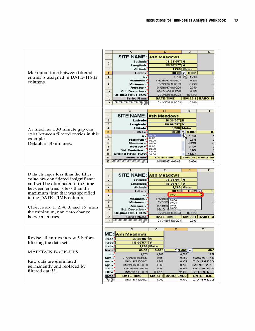
As much as a 30-minute gap canexist between filtered entries in thisexample.Default is 30 minutes.

Data changes less than the filtervalue are considered insignificantand will be eliminated if the timebetween entries is less than themaximum time that was specifiedin the DATE-TIME column.

Choices are 1, 2, 4, 8, and 16 timesthe minimum, non-zero changebetween entries.

Revise all entries in row 5 beforefiltering the data set.

MAINTAIN BACK-UPS

Raw data are eliminatedpermanently and replaced byfiltered data!!!

Maximum time between filteredentries is assigned in DATE-TIMEcolumns.


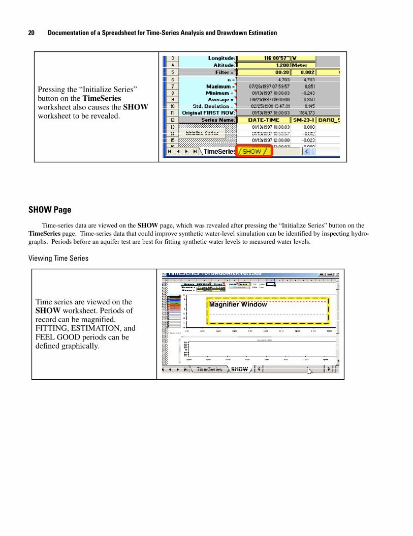
Pressing the “Initialize Series”button on the TimeSeriesworksheet also causes the SHOWworksheet to be revealed.

SHOW Page

Time-series data are viewed on the SHOW page, which was revealed after pressing the “Initialize Series” button on the TimeSeries page. Time-series data that could improve synthetic water-level simulation can be identified by inspecting hydro-graphs. Periods before an aquifer test are best for fitting synthetic water levels to measured water levels.

Viewing Time Series

Time series are viewed on theSHOW worksheet. Periods ofrecord can be magnified.FITTING, ESTIMATION, andFEEL GOOD periods can bedefined graphically.

Magnifier Window


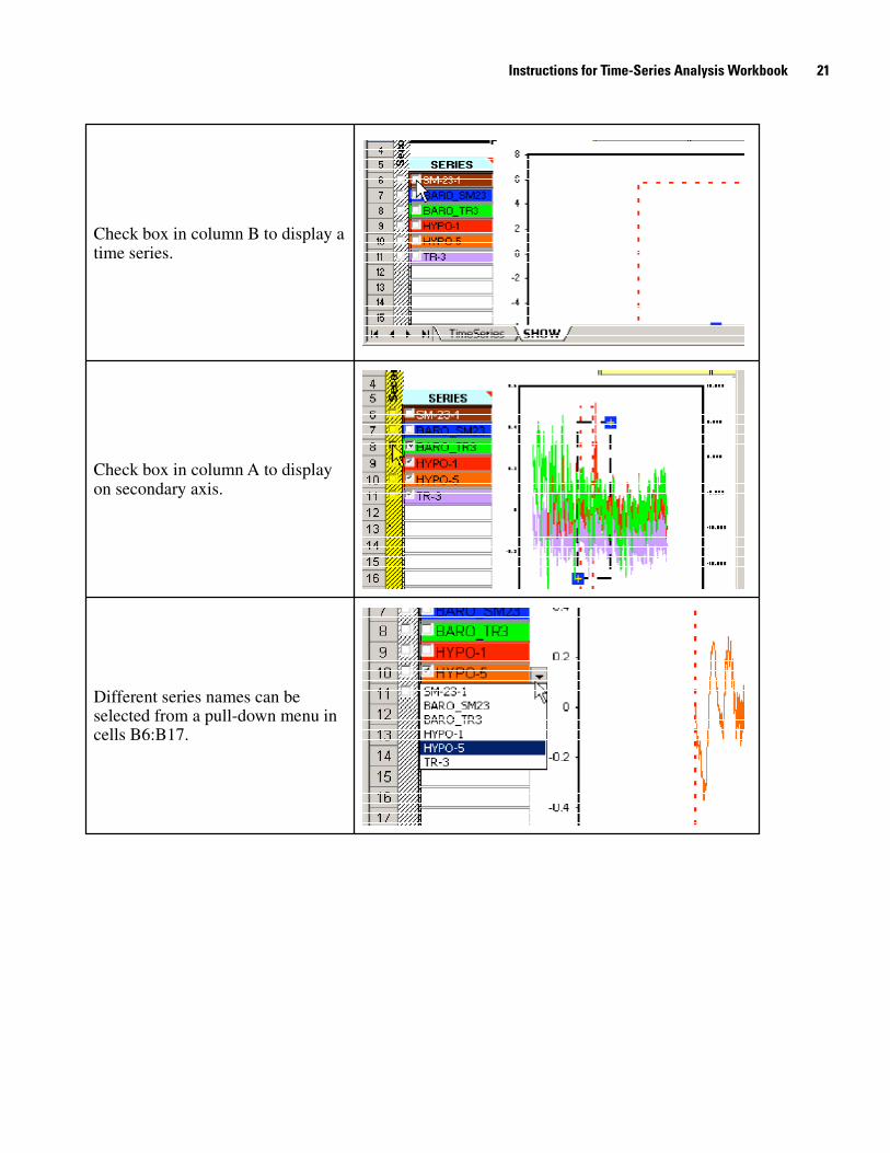
Different series names can beselected from a pull-down menu incells B6:B17.

Check box in column A to displayon secondary axis.

Check box in column B to display atime series.


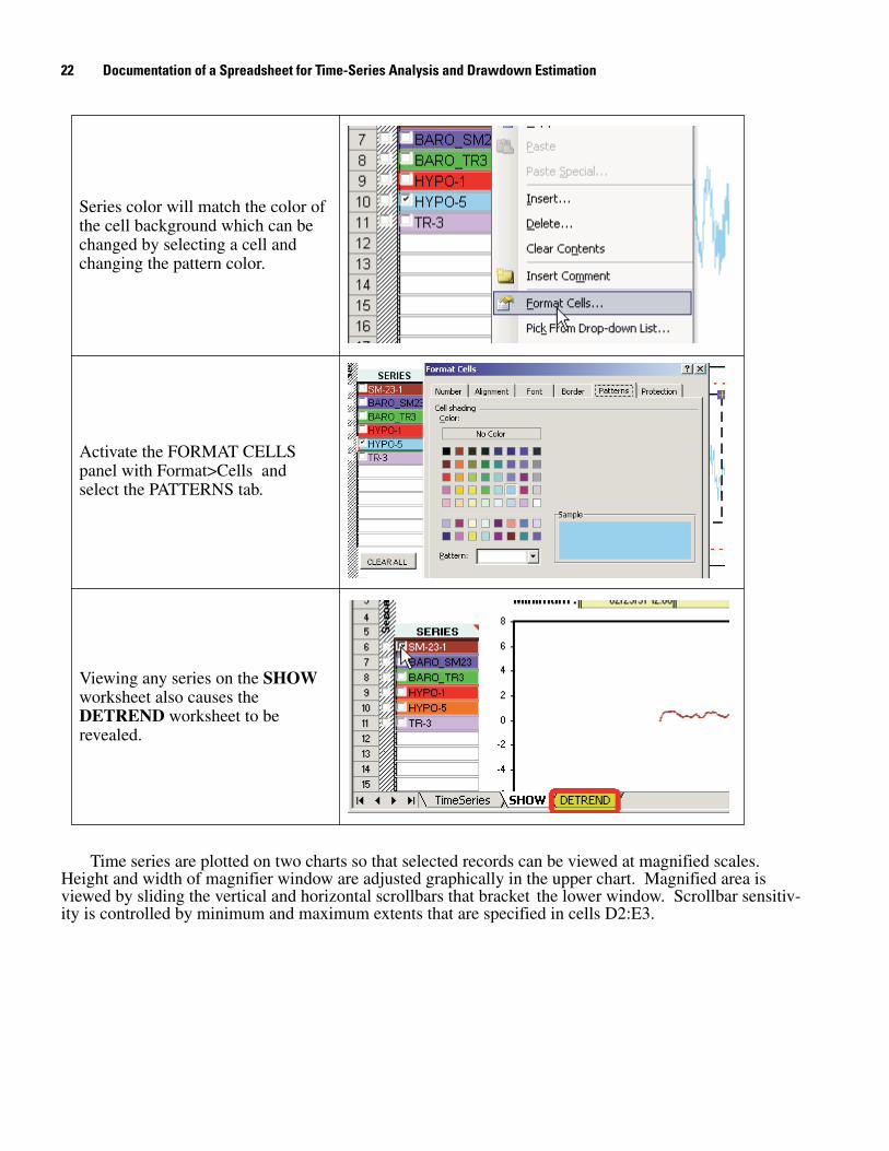
Series color will match the color ofthe cell background which can bechanged by selecting a cell andchanging the pattern color.

Activate the FORMAT CELLSpanel with Format>Cells andselect the PATTERNS tab.

Viewing any series on the SHOWworksheet also causes theDETREND worksheet to berevealed.

Time series are plotted on two charts so that selected records can be viewed at magnified scales. Height and width of magnifier window are adjusted graphically in the upper chart. Magnified area is viewed by sliding the vertical and horizontal scrollbars that bracket the lower window. Scrollbar sensitiv-ity is controlled by minimum and maximum extents that are specified in cells D2:E3.


Magnifying Selected Periods of Time Series

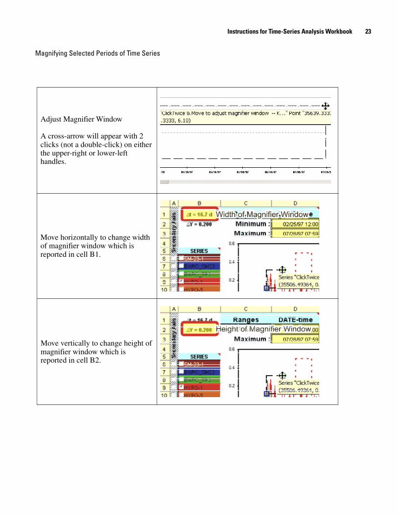
Move vertically to change height ofmagnifier window which isreported in cell B2.

Move horizontally to change widthof magnifier window which isreported in cell B1.

Adjust Magnifier Window

A cross-arrow will appear with 2clicks (not a double-click) on eitherthe upper-right or lower-lefthandles.


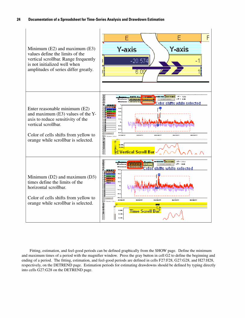
Minimum (E2) and maximum (E3)values define the limits of thevertical scrollbar. Range frequentlyis not initialized well whenamplitudes of series differ greatly.

Enter reasonable minimum (E2)and maximum (E3) values of the Y-axis to reduce sensitivity of thevertical scrollbar.

Color of cells shifts from yellow toorange while scrollbar is selected.

Minimum (D2) and maximum (D3)times define the limits of thehorizontal scrollbar.

Color of cells shifts from yellow toorange while scrollbar is selected.

Fitting, estimation, and feel-good periods can be defined graphically from the SHOW page. Define the minimum and maximum times of a period with the magnifier window. Press the gray button in cell G2 to define the beginning and ending of a period. The fitting, estimation, and feel-good periods are defined in cells F27:F28, G27:G28, and H27:H28, respectively, on the DETREND page. Estimation periods for estimating drawdowns should be defined by typing directly into cells G27:G28 on the DETREND page.


Graphically Defining Fitting, Estimation, and Feel-Good Periods

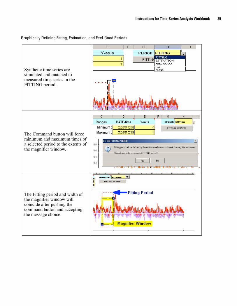
Synthetic time series aresimulated and matched tomeasured time series in theFITTING period.

The Command button will forceminimum and maximum times ofa selected period to the extents ofthe magnifier window.

The Fitting period and width ofthe magnifier window willcoincide after pushing thecommand button and acceptingthe message choice.


DETREND Page

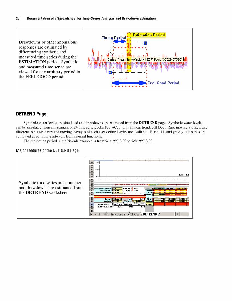
Synthetic water levels are simulated and drawdowns are estimated from the DETREND page. Synthetic water levels can be simulated from a maximum of 24 time series, cells F33:AC33, plus a linear trend, cell D32. Raw, moving average, and differences between raw and moving averages of each user-defined series are available. Earth-tide and gravity-tide series are computed at 30-minute intervals from internal functions.

The estimation period in the Nevada example is from 5/1/1997 8:00 to 5/5/1997 8:00.

Major Features of the DETREND Page

Drawdowns or other anomalousresponses are estimated bydifferencing synthetic andmeasured time series during theESTIMATION period. Syntheticand measured time series areviewed for any arbitrary period inthe FEEL GOOD period.

Synthetic time series are simulatedand drawdowns are estimated fromthe DETREND worksheet.


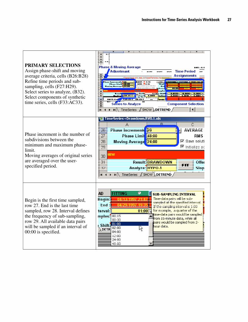
Begin is the first time sampled,row 27. End is the last timesampled, row 28. Interval definesthe frequency of sub-sampling,row 29. All available data pairswill be sampled if an interval of00:00 is specified.

Phase increment is the number ofsubdivisions between theminimum and maximum phase-limit.Moving averages of original seriesare averaged over the user-specified period.

PRIMARY SELECTIONSAssign phase-shift and movingaverage criteria, cells (B26:B28)Refine time periods and sub-sampling, cells (F27:H29).Select series to analyze, (B32).Select components of synthetictime series, cells (F33:AC33).


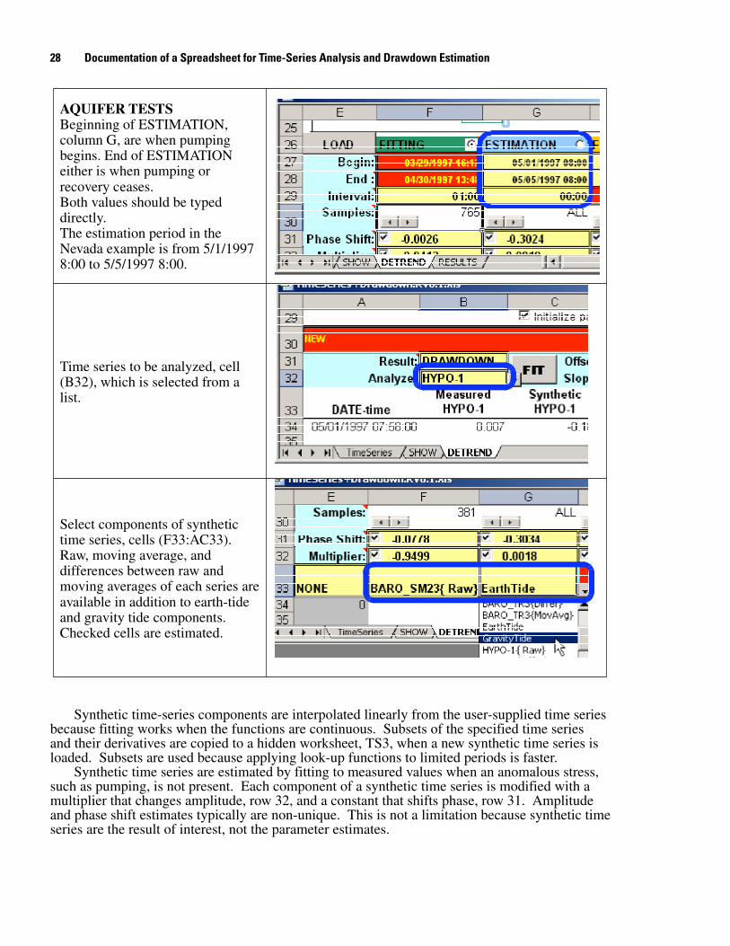
Select components of synthetictime series, cells (F33:AC33).Raw, moving average, anddifferences between raw andmoving averages of each series areavailable in addition to earth-tideand gravity tide components.Checked cells are estimated.

Time series to be analyzed, cell(B32), which is selected from alist.

AQUIFER TESTSBeginning of ESTIMATION,column G, are when pumpingbegins. End of ESTIMATIONeither is when pumping orrecovery ceases.Both values should be typeddirectly.The estimation period in theNevada example is from 5/1/19978:00 to 5/5/1997 8:00.

Synthetic time-series components are interpolated linearly from the user-supplied time series because fitting works when the functions are continuous. Subsets of the specified time series and their derivatives are copied to a hidden worksheet, TS3, when a new synthetic time series is loaded. Subsets are used because applying look-up functions to limited periods is faster.

Synthetic time series are estimated by fitting to measured values when an anomalous stress, such as pumping, is not present. Each component of a synthetic time series is modified with a multiplier that changes amplitude, row 32, and a constant that shifts phase, row 31. Amplitude and phase shift estimates typically are non-unique. This is not a limitation because synthetic time series are the result of interest, not the parameter estimates.

2� Documentation of a Spreadsheet for Time-Series Analysis and Drawdown Estimation

Loading and Fitting Synthetic Series

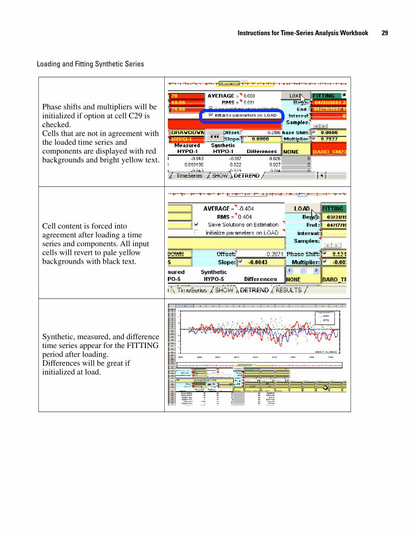
Synthetic, measured, and differencetime series appear for the FITTINGperiod after loading.Differences will be great ifinitialized at load.

Cell content is forced intoagreement after loading a timeseries and components. All inputcells will revert to pale yellowbackgrounds with black text.

Phase shifts and multipliers will beinitialized if option at cell C29 ischecked.Cells that are not in agreement withthe loaded time series andcomponents are displayed with redbackgrounds and bright yellow text.


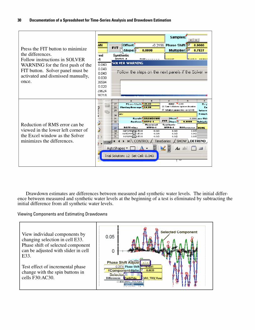
Drawdown estimates are differences between measured and synthetic water levels. The initial differ-ence between measured and synthetic water levels at the beginning of a test is eliminated by subtracting the initial difference from all synthetic water levels.

Viewing Components and Estimating Drawdowns

Reduction of RMS error can beviewed in the lower left corner ofthe Excel window as the Solverminimizes the differences.

Press the FIT button to minimizethe differences.Follow instructions in SOLVERWARNING for the first push of theFIT button. Solver panel must beactivated and dismissed manually,once.

View individual components bychanging selection in cell E33.Phase shift of selected componentcan be adjusted with slider in cellE33.

Test effect of incremental phasechange with the spin buttons incells F30:AC30.

�0 Documentation of a Spreadsheet for Time-Series Analysis and Drawdown Estimation

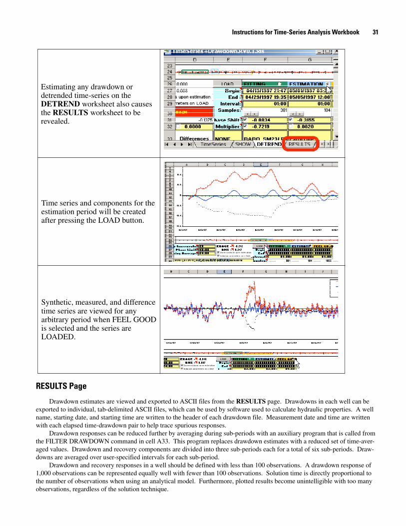
Synthetic, measured, and differencetime series are viewed for anyarbitrary period when FEEL GOODis selected and the series areLOADED.

Time series and components for theestimation period will be createdafter pressing the LOAD button.

Estimating any drawdown ordetrended time-series on theDETREND worksheet also causesthe RESULTS worksheet to berevealed.

RESULTS Page

Drawdown estimates are viewed and exported to ASCII files from the RESULTS page. Drawdowns in each well can be exported to individual, tab-delimited ASCII files, which can be used by software used to calculate hydraulic properties. A well name, starting date, and starting time are written to the header of each drawdown file. Measurement date and time are written with each elapsed time-drawdown pair to help trace spurious responses.

Drawdown responses can be reduced further by averaging during sub-periods with an auxiliary program that is called from the FILTER DRAWDOWN command in cell A33. This program replaces drawdown estimates with a reduced set of time-aver-aged values. Drawdown and recovery components are divided into three sub-periods each for a total of six sub-periods. Draw-downs are averaged over user-specified intervals for each sub-period.

Drawdown and recovery responses in a well should be defined with less than 100 observations. A drawdown response of 1,000 observations can be represented equally well with fewer than 100 observations. Solution time is directly proportional to the number of observations when using an analytical model. Furthermore, plotted results become unintelligible with too many observations, regardless of the solution technique.

Instructions for Time-Series Analysis Workbook �1

These drawdown estimates are analyzed by copying directly from the spreadsheet application or writing the results to tab-delimited ASCII files.

Viewing, Filtering, and Exporting Drawdowns

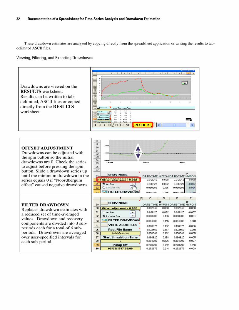
Drawdowns are viewed on theRESULTS worksheet.Results can be written to tab-delimited, ASCII files or copieddirectly from the RESULTSworksheet.

FILTER DRAWDOWNReplaces drawdown estimates witha reduced set of time-averagedvalues. Drawdown and recoverycomponents are divided into 3 sub-periods each for a total of 6 sub-periods. Drawdowns are averagedover user-specified intervals foreach sub-period.

OFFSET ADJUSTMENTDrawdowns can be adjusted withthe spin button so the initialdrawdowns are 0. Check the seriesto adjust before pressing the spinbutton. Slide a drawdown series upuntil the minimum drawdown in theseries equals 0 if "Noordbergumeffect" caused negative drawdowns.


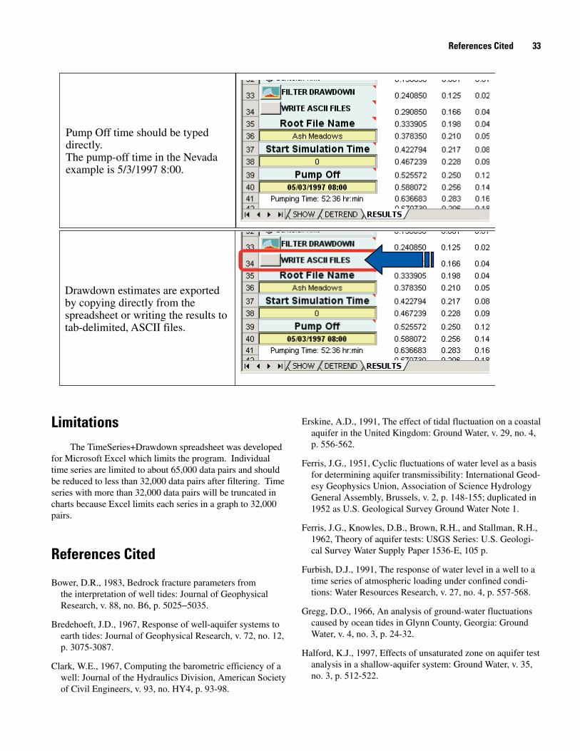
Drawdown estimates are exportedby copying directly from thespreadsheet or writing the results totab-delimited, ASCII files.

Pump Off time should be typeddirectly.The pump-off time in the Nevadaexample is 5/3/1997 8:00.

LimitationsThe TimeSeries+Drawdown spreadsheet was developed

for Microsoft Excel which limits the program. Individual time series are limited to about 65,000 data pairs and should be reduced to less than 32,000 data pairs after filtering. Time series with more than 32,000 data pairs will be truncated in charts because Excel limits each series in a graph to 32,000 pairs.

References Cited

Bower, D.R., 1983, Bedrock fracture parameters from the interpretation of well tides: Journal of Geophysical Research, v. 88, no. B6, p. 5025–5035.

Bredehoeft, J.D., 1967, Response of well-aquifer systems to earth tides: Journal of Geophysical Research, v. 72, no. 12, p. 3075-3087.

Clark, W.E., 1967, Computing the barometric efficiency of a well: Journal of the Hydraulics Division, American Society of Civil Engineers, v. 93, no. HY4, p. 93-98.

Erskine, A.D., 1991, The effect of tidal fluctuation on a coastal aquifer in the United Kingdom: Ground Water, v. 29, no. 4, p. 556-562.

Ferris, J.G., 1951, Cyclic fluctuations of water level as a basis for determining aquifer transmissibility: International Geod-esy Geophysics Union, Association of Science Hydrology General Assembly, Brussels, v. 2, p. 148-155; duplicated in 1952 as U.S. Geological Survey Ground Water Note 1.

Ferris, J.G., Knowles, D.B., Brown, R.H., and Stallman, R.H., 1962, Theory of aquifer tests: USGS Series: U.S. Geologi-cal Survey Water Supply Paper 1536-E, 105 p.

Furbish, D.J., 1991, The response of water level in a well to a time series of atmospheric loading under confined condi-tions: Water Resources Research, v. 27, no. 4, p. 557-568.

Gregg, D.O., 1966, An analysis of ground-water fluctuations caused by ocean tides in Glynn County, Georgia: Ground Water, v. 4, no. 3, p. 24-32.

Halford, K.J., 1997, Effects of unsaturated zone on aquifer test analysis in a shallow-aquifer system: Ground Water, v. 35, no. 3, p. 512-522.

References Cited ��

Hanson, J.M., and Owen, L.B., 1982, Fracture orientation analysis by the solid earth tidal strain method: Presented at the 57th Annual Fall Technical Conference and Exhibition of the Society of Petroleum Engineers of AIME, American Institute of Mechanical Engineers, New Orleans, Louisiana, September 26-29, 1982.

Harrison, J.C., 1971, New computer programs for the calcu-lation of Earth tides: National Oceanic and Atmospheric Administration/University of Colorado, Cooperative Insti-tute for Research in Environmental Sciences, 30 p.

Hsieh, P.A., Bredehoeft, J.D., and Rojstaczer, S.A., 1988, Response of well-aquifer systems to earth tides: Problem revisited: Water Resources Research, v. 24, no. 3, p. 468-472.

Jacob, C.E., 1940, On the flow of water in an elastic artesian aquifer: American Geophysical Union Transactions, part 2, p. 574-586; duplicated in 1953 as U.S. Geological Survey Ground Water Note 8.

Jiao, J.J., and Tang, Z., 1999, An analytic solution of ground-water response to tidal fluctuation in a leaky confined aqui-fer: Water Resources Research, v. 35, no. 3, p. 747-751.

Kruseman, G.P., and DeRidder, N.A., 1990, Analysis and evaluation of pumping test data, Publication 47, (2nd ed.): Wageningen, The Netherlands, International Institute for Land Reclamation and Improvement, 370 p.

Li, H., and Jiao, J.J., 2001, Tide-induced groundwater fluctua-tion in a coastal leaky confined aquifer system extending under the sea: Water Resources Research, v. 37, no. 5, p. 1165-1171.

Marine, I.W., 1975, Water level fluctuations due to earth tides in a well pumping from slightly fractured rock: Water Resources Research, v. 11, no. 1, p. 165-173.

Melchior, P., 1964, Earth tides, in Odishaw, H., ed., Research in Geophysics, v. 2: Cambridge, Massachusetts, Massachu-setts Institute of Technology Press, p. 183-193.

Merritt, M.L., 2004, Estimating hydraulic properties of the Floridan aquifer system by analysis of earth-tide, ocean-tide, and barometric effects, Collier and Hendry Counties, Florida: U.S. Geological Survey Water-Resources Investiga-tions Report 03-4267, 70 p.

Narasimhan, T.N., Kanehiro, B.Y., and Witherspoon, P.A., 1984, Interpretation of earth tide responses of three deep, confined aquifers: Journal of Geophysical Research, v. 89, no. B3, p. 1913-1924.

O’Reilly, A.M., 1998, Hydrogeology and simulation of the effects of reclaimed-water application in west Orange and southeast Lake Counties, Florida: U.S. Geological Survey Water-Resources Investigations Report 97-4199, 91 p.

Risser, D.W., and Bird, P.H., 2003, Aquifer tests and simula-tion of ground-water flow in Triassic sedimentary rocks near Colmar, Bucks, and Montgomery Counties, Pennsylva-nia: U.S. Geological Survey Water-Resources Investigations Report 03-4159, 73 p.

Robinson, E.S., and Bell, R.T., 1971, Tides in confined well-aquifer systems: Journal of Geophysical Research, v. 76, no. 8, p. 1857-1869.

Rojstaczer, S., 1988, Determination of fluid flow properties from the response of water levels in wells to atmospheric loading: Water Resources Research, v. 24, no. 11, p. 1927-1938.

Rojstaczer, S., and Agnew, D.C., 1989, The influence of for-mation material properties on the response of water levels in wells to earth tides and atmospheric loading: Journal of Geophysical Research, v. 94, no. B9, p. 12403-12411.

Rojstaczer, S., and Riley, F.S., 1990, Response of the water level in a well to earth tides and atmospheric loading under unconfined conditions: Water Resources Research, v. 26, no. 8, p. 1803-1817.

Rutledge, A.T., 1985, Use of double-mass curves to deter-mine drawdown in a long-term aquifer test in north-central Volusia County, Florida: U.S. Geological Survey Water-Resources Investigations Report 84-4309, 29 p.

Theis, C.V., 1935, The relation between the lowering of the piezometric surface and the rate and duration of discharge of a well using ground water storage: Transactions of the American Geophysical Union, v. 16, p. 519–524.

van der Kamp, G., 1972, Tidal fluctuations in a confined aquifer extending under the sea: International Geological Congress, v. 24, no. 11, p. 101-106.

van der Kamp, G., and Gale, J.E., 1983, Theory of earth tide and barometric effects in porous formations with compress-ible grains: Water Resources Research, v. 19, no. 2, p. 538-544.

Verruijt, A., 1969, Elastic storage of aquifers, in De Wiest, R.J.M., ed., Flow Through Porous Media: New York, Aca-demic Press, p. 331-376.

Weeks, E.P., 1979, Barometric fluctuations in wells tapping deep unconfined aquifers: Water Resources Research, v. 15, no. 5, p. 1167-1176.

Wolff, R.G., 1970, Relationship between horizontal strain near a well and reverse water level fluctuation: Water Resources Research, v. 6, p. 1721-1728.


Appendix

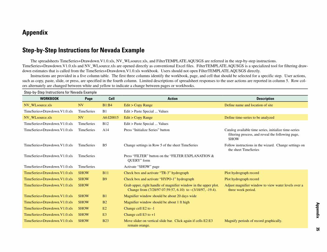
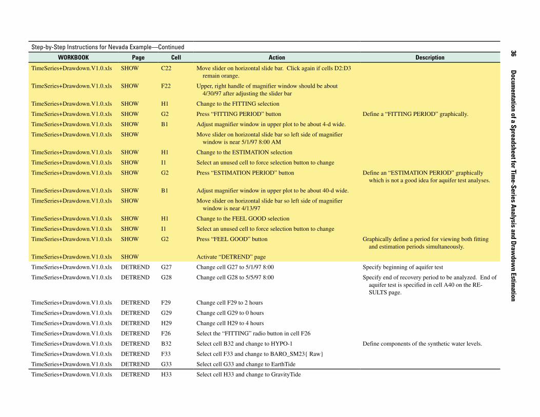
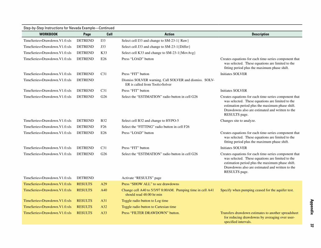
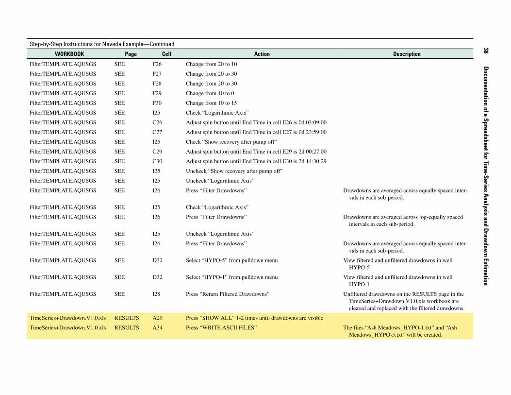
Step-by-Step Instructions for Nevada ExampleThe spreadsheets TimeSeries+Drawdown.V1.0.xls, NV_WLsource.xls, and FilterTEMPLATE.AQUSGS are referred in the step-by-step instructions.

TimeSeries+Drawdown.V1.0.xls and NV_WLsource.xls are opened directly as conventional Excel files. FilterTEMPLATE.AQUSGS is a specialized tool for filtering draw-down estimates that is called from the TimeSeries+Drawdown.V1.0.xls workbook. Users should not open FilterTEMPLATE.AQUSGS directly.

Instructions are provided in a five column table. The first three columns identify the workbook, page, and cell that should be selected for a specific step. User actions, such as copy, paste, slide, or press, are specified in the fourth column. Limited descriptions of spreadsheet responses to the user actions are reported in column 5. Row col-ors alternately are changed between white and yellow to indicate a change between pages or workbooks.

Step-by-Step Instructions for Nevada Example—Continued

WORKBOOK Page Cell Action Description

NV_WLsource.xls NV B1:B4 Edit > Copy Range Define name and location of site

TimeSeries+Drawdown.V1.0.xls TimeSeries B1 Edit > Paste Special ... Values

NV_WLsource.xls NV A6:I20015 Edit > Copy Range Define time-series to be analyzed

TimeSeries+Drawdown.V1.0.xls TimeSeries B12 Edit > Paste Special ... Values

TimeSeries+Drawdown.V1.0.xls TimeSeries A14 Press “Initialize Series” button Catalog available time series, initialize time-series filtering process, and reveal the following page, SHOW

TimeSeries+Drawdown.V1.0.xls TimeSeries B5 Change settings in Row 5 of the sheet TimeSeries Follow instructions in the wizard. Change settings on the sheet TimeSeries

TimeSeries+Drawdown.V1.0.xls TimeSeries Press “FILTER” button on the “FILTER EXPLANATION & QUERY” form

TimeSeries+Drawdown.V1.0.xls TimeSeries Activate “SHOW” page

TimeSeries+Drawdown.V1.0.xls SHOW B11 Check box and activate “TR-3” hydrograph Plot hydrograph record

TimeSeries+Drawdown.V1.0.xls SHOW B9 Check box and activate “HYPO-1” hydrograph Plot hydrograph record

TimeSeries+Drawdown.V1.0.xls SHOW Grab upper, right handle of magnifier window in the upper plot. Change from (7/28/97 07:59:57, 6.10) to ~(3/18/97, -19.4).

Adjust magnifier window to view water levels over a three week period.

TimeSeries+Drawdown.V1.0.xls SHOW B1 Magnifier window should be about 20 days wide

TimeSeries+Drawdown.V1.0.xls SHOW B2 Magnifier window should be about 1 ft high

TimeSeries+Drawdown.V1.0.xls SHOW E2 Change cell E2 to -1

TimeSeries+Drawdown.V1.0.xls SHOW E3 Change cell E3 to +1

TimeSeries+Drawdown.V1.0.xls SHOW B23 Move slider on vertical slide bar. Click again if cells E2:E3 remain orange.

Magnify periods of record graphically.

Appendix

�5

�6

Documentation of a Spreadsheet for Tim

e-Series Analysis and Drawdow

n Estimation



TimeSeries+Drawdown.V1.0.xls SHOW C22 Move slider on horizontal slide bar. Click again if cells D2:D3 remain orange.

TimeSeries+Drawdown.V1.0.xls SHOW F22 Upper, right handle of magnifier window should be about 4/30/97 after adjusting the slider bar

TimeSeries+Drawdown.V1.0.xls SHOW H1 Change to the FITTING selection

TimeSeries+Drawdown.V1.0.xls SHOW G2 Press “FITTING PERIOD” button Define a “FITTING PERIOD” graphically.

TimeSeries+Drawdown.V1.0.xls SHOW B1 Adjust magnifier window in upper plot to be about 4-d wide.

TimeSeries+Drawdown.V1.0.xls SHOW Move slider on horizontal slide bar so left side of magnifier window is near 5/1/97 8:00 AM

TimeSeries+Drawdown.V1.0.xls SHOW H1 Change to the ESTIMATION selection

TimeSeries+Drawdown.V1.0.xls SHOW I1 Select an unused cell to force selection button to change

TimeSeries+Drawdown.V1.0.xls SHOW G2 Press “ESTIMATION PERIOD” button Define an “ESTIMATION PERIOD” graphically which is not a good idea for aquifer test analyses.

TimeSeries+Drawdown.V1.0.xls SHOW B1 Adjust magnifier window in upper plot to be about 40-d wide.

TimeSeries+Drawdown.V1.0.xls SHOW Move slider on horizontal slide bar so left side of magnifier window is near 4/13/97

TimeSeries+Drawdown.V1.0.xls SHOW H1 Change to the FEEL GOOD selection

TimeSeries+Drawdown.V1.0.xls SHOW I1 Select an unused cell to force selection button to change

TimeSeries+Drawdown.V1.0.xls SHOW G2 Press “FEEL GOOD” button Graphically define a period for viewing both fitting and estimation periods simultaneously.

TimeSeries+Drawdown.V1.0.xls SHOW Activate “DETREND” page

TimeSeries+Drawdown.V1.0.xls DETREND G27 Change cell G27 to 5/1/97 8:00 Specify beginning of aquifer test

TimeSeries+Drawdown.V1.0.xls DETREND G28 Change cell G28 to 5/5/97 8:00 Specify end of recovery period to be analyzed. End of aquifer test is specified in cell A40 on the RE-SULTS page.

TimeSeries+Drawdown.V1.0.xls DETREND F29 Change cell F29 to 2 hours

TimeSeries+Drawdown.V1.0.xls DETREND G29 Change cell G29 to 0 hours

TimeSeries+Drawdown.V1.0.xls DETREND H29 Change cell H29 to 4 hours

TimeSeries+Drawdown.V1.0.xls DETREND F26 Select the “FITTING” radio button in cell F26

TimeSeries+Drawdown.V1.0.xls DETREND B32 Select cell B32 and change to HYPO-1 Define components of the synthetic water levels.

TimeSeries+Drawdown.V1.0.xls DETREND F33 Select cell F33 and change to BARO_SM23{ Raw}

TimeSeries+Drawdown.V1.0.xls DETREND G33 Select cell G33 and change to EarthTide

TimeSeries+Drawdown.V1.0.xls DETREND H33 Select cell H33 and change to GravityTide



TimeSeries+Drawdown.V1.0.xls DETREND I33 Select cell I33 and change to SM-23-1{ Raw}

TimeSeries+Drawdown.V1.0.xls DETREND J33 Select cell J33 and change to SM-23-1{Differ}

TimeSeries+Drawdown.V1.0.xls DETREND K33 Select cell K33 and change to SM-23-1{MovAvg}

TimeSeries+Drawdown.V1.0.xls DETREND E26 Press “LOAD” button Creates equations for each time-series component that was selected. These equations are limited to the fitting period plus the maximum phase shift.

TimeSeries+Drawdown.V1.0.xls DETREND C31 Press “FIT” button Initiates SOLVER

TimeSeries+Drawdown.V1.0.xls DETREND Dismiss SOLVER warning. Call SOLVER and dismiss. SOLV-ER is called from Tools>Solver


TimeSeries+Drawdown.V1.0.xls DETREND G26 Select the “ESTIMATION” radio button in cell G26 Creates equations for each time-series component that was selected. These equations are limited to the estimation period plus the maximum phase shift. Drawdowns also are estimated and written to the RESULTS page.

TimeSeries+Drawdown.V1.0.xls DETREND B32 Select cell B32 and change to HYPO-5 Changes site to analyze.

TimeSeries+Drawdown.V1.0.xls DETREND F26 Select the “FITTING” radio button in cell F26

TimeSeries+Drawdown.V1.0.xls DETREND E26 Press “LOAD” button Creates equations for each time-series component that was selected. These equations are limited to the fitting period plus the maximum phase shift.


TimeSeries+Drawdown.V1.0.xls DETREND G26 Select the “ESTIMATION” radio button in cell G26 Creates equations for each time-series component that was selected. These equations are limited to the estimation period plus the maximum phase shift. Drawdowns also are estimated and written to the RESULTS page.

TimeSeries+Drawdown.V1.0.xls DETREND Activate “RESULTS” page

TimeSeries+Drawdown.V1.0.xls RESULTS A29 Press “SHOW ALL” to see drawdowns

TimeSeries+Drawdown.V1.0.xls RESULTS A40 Change cell A40 to 5/3/97 8:00AM. Pumping time in cell A41 should read 48:00 hr:min

Specify when pumping ceased for the aquifer test.

TimeSeries+Drawdown.V1.0.xls RESULTS A31 Toggle radio button to Log time

TimeSeries+Drawdown.V1.0.xls RESULTS A32 Toggle radio button to Cartesian time

TimeSeries+Drawdown.V1.0.xls RESULTS A33 Press “FILTER DRAWDOWN” button. Transfers drawdown estimates to another spreadsheet for reducing drawdowns by averaging over user-specified intervals.

Appendix

��

��

Documentation of a Spreadsheet for Tim

e-Series Analysis and Drawdow

n Estimation



FilterTEMPLATE.AQUSGS SEE F26 Change from 20 to 10





FilterTEMPLATE.AQUSGS SEE I25 Check “Logarithmic Axis”

FilterTEMPLATE.AQUSGS SEE C26 Adjust spin button until End Time in cell E26 is 0d 03:09:00


FilterTEMPLATE.AQUSGS SEE I25 Check “Show recovery after pump off”



FilterTEMPLATE.AQUSGS SEE I25 Uncheck “Show recovery after pump off”

FilterTEMPLATE.AQUSGS SEE I25 Uncheck “Logarithmic Axis”

FilterTEMPLATE.AQUSGS SEE I26 Press “Filter Drawdowns” Drawdowns are averaged across equally spaced inter-vals in each sub-period.

FilterTEMPLATE.AQUSGS SEE I25 Check “Logarithmic Axis”

FilterTEMPLATE.AQUSGS SEE I26 Press “Filter Drawdowns” Drawdowns are averaged across log-equally spaced intervals in each sub-period.

FilterTEMPLATE.AQUSGS SEE I25 Uncheck “Logarithmic Axis”

FilterTEMPLATE.AQUSGS SEE I26 Press “Filter Drawdowns” Drawdowns are averaged across equally spaced inter-vals in each sub-period.

FilterTEMPLATE.AQUSGS SEE D32 Select “HYPO-5” from pulldown menu View filtered and unfiltered drawdowns in well HYPO-5

FilterTEMPLATE.AQUSGS SEE D32 Select “HYPO-1” from pulldown menu View filtered and unfiltered drawdowns in well HYPO-1

FilterTEMPLATE.AQUSGS SEE I28 Press “Return Filtered Drawdowns” Unfiltered drawdowns on the RESULTS page in the TimeSeries+Drawdown.V1.0.xls workbook are cleared and replaced with the filtered drawdowns.

TimeSeries+Drawdown.V1.0.xls RESULTS A29 Press “SHOW ALL” 1-2 times until drawdowns are visible

TimeSeries+Drawdown.V1.0.xls RESULTS A34 Press “WRITE ASCII FILES” The files “Ash Meadows_HYPO-1.txt” and “Ash Meadows_HYPO-5.txt” will be created.

HA

LFORD

—D

ocumentation of a Spreadsheet for Tim

e-Series Analysis and D

rawdow

n Estimation—

SIR 2006-5024

Documents

Documentation of a Spreadsheet for Time-Series Analysis ... · Documentation of a Spreadsheet for Time-Series Analysis and Drawdown Estimation By Keith J. Halford U.S. Department