Embed Size (px)
Citation preview
Documentation for VP:
Nonlinear Vlasov-Poisson Simulation Code
2016
i

ii
Contents
1 Theory for Landau Damping in a 1D1V Vlasov-Poisson Plasma 1
1.1 Vlasov-Poisson Problem . . . . . . . . . . . . . . . . . . . . . . . . . . . . . . . . . . . . . . . . . . . . . . 1
1.2 Derivation of Poynting’s Theorem and Electrostatic Limit . . . . . . . . . . . . . . . . . . . . . . . . . . . 1
1.3 Conservation of Energy in the 1D1V Vlasov-Poisson System . . . . . . . . . . . . . . . . . . . . . . . . . . 3
1.4 Transfer of Energy in Collisionless Wave-Particle Interactions . . . . . . . . . . . . . . . . . . . . . . . . . 4
1.4.1 Implications for Linear vs. Nonlinear Energy Conservation . . . . . . . . . . . . . . . . . . . . . . . 6
1.4.2 Diagnostics of the Energy Transfer to Particles . . . . . . . . . . . . . . . . . . . . . . . . . . . . . 6
1.4.3 Ballistic Perturbation Gains No Energy . . . . . . . . . . . . . . . . . . . . . . . . . . . . . . . . . 8
1.4.4 Relation to Field-Particle Correlations . . . . . . . . . . . . . . . . . . . . . . . . . . . . . . . . . . 8
1.4.5 Note to Self . . . . . . . . . . . . . . . . . . . . . . . . . . . . . . . . . . . . . . . . . . . . . . . . . 9
1.4.6 References on Wave-Particle Correlations in the Literature . . . . . . . . . . . . . . . . . . . . . . 9
2 Numerical Implementation of VP: Nonlinear Vlasov-Poisson Simulation Code 11
2.1 Overview of Code Implementation . . . . . . . . . . . . . . . . . . . . . . . . . . . . . . . . . . . . . . . . 11
2.2 Vlasov-Poisson Problem . . . . . . . . . . . . . . . . . . . . . . . . . . . . . . . . . . . . . . . . . . . . . . 11
2.2.1 Separating Linear and Nonlinear Terms . . . . . . . . . . . . . . . . . . . . . . . . . . . . . . . . . 11
2.2.2 Separating Ballistic and Wave Terms . . . . . . . . . . . . . . . . . . . . . . . . . . . . . . . . . . . 12
2.3 Green’s Function Solution for Electrostatic Potential . . . . . . . . . . . . . . . . . . . . . . . . . . . . . . 12
2.4 Normalization . . . . . . . . . . . . . . . . . . . . . . . . . . . . . . . . . . . . . . . . . . . . . . . . . . . . 13
2.4.1 Energy Diagnostic Normalization . . . . . . . . . . . . . . . . . . . . . . . . . . . . . . . . . . . . . 15
2.5 Notes on VP2 (Multispecies and drifts) and VP3 (Krook Collisions) Implementation . . . . . . . . . . . . 15
2.6 Numerical Discretization . . . . . . . . . . . . . . . . . . . . . . . . . . . . . . . . . . . . . . . . . . . . . . 15
2.6.1 3rd-Order Adams-Bashforth Timestepping . . . . . . . . . . . . . . . . . . . . . . . . . . . . . . . . 15
2.6.2 Spatial and Velocity Derivatives . . . . . . . . . . . . . . . . . . . . . . . . . . . . . . . . . . . . . 15
2.7 Initial Conditions . . . . . . . . . . . . . . . . . . . . . . . . . . . . . . . . . . . . . . . . . . . . . . . . . . 16
2.7.1 Initialization of Electron Density Perturbation . . . . . . . . . . . . . . . . . . . . . . . . . . . . . 16
2.7.2 Linear Wave Eigenfunction . . . . . . . . . . . . . . . . . . . . . . . . . . . . . . . . . . . . . . . . 16
2.7.3 Localized Wavepacket . . . . . . . . . . . . . . . . . . . . . . . . . . . . . . . . . . . . . . . . . . . 19
iii
2.8 Notes . . . . . . . . . . . . . . . . . . . . . . . . . . . . . . . . . . . . . . . . . . . . . . . . . . . . . . . . 19
3 Results for Landau Damping from VP: Nonlinear Vlasov-Poisson Simulation Code 21
3.1 Two Test Cases . . . . . . . . . . . . . . . . . . . . . . . . . . . . . . . . . . . . . . . . . . . . . . . . . . . 21
3.2 Identification through Correlations . . . . . . . . . . . . . . . . . . . . . . . . . . . . . . . . . . . . . . . . 23
3.3 Numerical Recurrence in Linear Run . . . . . . . . . . . . . . . . . . . . . . . . . . . . . . . . . . . . . . . 27
3.4 Linear Run Comments . . . . . . . . . . . . . . . . . . . . . . . . . . . . . . . . . . . . . . . . . . . . . . . 29
3.5 Nonlinear Run Comments . . . . . . . . . . . . . . . . . . . . . . . . . . . . . . . . . . . . . . . . . . . . . 29
3.6 Final Strategy . . . . . . . . . . . . . . . . . . . . . . . . . . . . . . . . . . . . . . . . . . . . . . . . . . . . 30
3.6.1 Two Cases: Moderately and Weakly Damped Langmuir Waves . . . . . . . . . . . . . . . . . . . . 30
3.6.2 UPDATED: Theory for Final Strategy . . . . . . . . . . . . . . . . . . . . . . . . . . . . . . . . . . 36
3.6.3 Theory for Final Strategy . . . . . . . . . . . . . . . . . . . . . . . . . . . . . . . . . . . . . . . . . 36
3.6.4 Results for Weakly Damped Case . . . . . . . . . . . . . . . . . . . . . . . . . . . . . . . . . . . . . 38
3.6.5 Results for Moderately Damped Case . . . . . . . . . . . . . . . . . . . . . . . . . . . . . . . . . . 41
3.6.6 Work to do with Correlations . . . . . . . . . . . . . . . . . . . . . . . . . . . . . . . . . . . . . . . 46
3.7 Line Plots of Contributions to δws(x0, v, t)/δt . . . . . . . . . . . . . . . . . . . . . . . . . . . . . . . . . . 47
3.8 Notes . . . . . . . . . . . . . . . . . . . . . . . . . . . . . . . . . . . . . . . . . . . . . . . . . . . . . . . . 51
iv
Chapter 1
Theory for Landau Damping in a 1D1VVlasov-Poisson Plasma
The main goal of these analytical calculations is to identify the energy transferred from the electrostatic field to the parti-
cles via resonant collisionless wave-particle interactions, and to determine the impact of this resonantly transferred energy
on the particle distribution functions. This theoretical insight will be used to devise novel analysis strategies to defini-
tively identify the action of collisionless wave-particle interactions in heliospheric plasmas using spacecraft measurements
or nonlinear kinetic numerical simulations.
Note, of course, that the Lorentz term in the Vlasov equation, in addition to governing resonant energy transfer in
collisionless wave-particle interactions, also is responsible for the typical oscillatory transfer of energy between fields and
particles characteristic of (linear) wave motion. Thus, the problem is to isolate the physics describing the resonant energy
transfer from the common linear wave response.
1.1 Vlasov-Poisson Problem
The 1D-1V Vlasov-Poisson system is governed by the Boltzmann equation for the species distribution functions fs(x, v, t)
∂fs∂t
+ v∂fs∂x
−qsms
∂φ
∂x
∂fs∂v
= 0 (1.1)
and the Poisson equation for the scalar electrostatic potential φ(x, t)
∂2φ
∂x2= −4π
∑
s
∫ +∞
−∞
dv qsfs (1.2)
1.2 Derivation of Poynting’s Theorem and Electrostatic Limit
Poynting’s theorem is derived directly from Maxwell’s equations, specifically Faraday’s Law
∂B
∂t= −c∇×E (1.3)
1
and the Ampere-Maxwell Law,
∂E
∂t= c∇×B− 4πj. (1.4)
First, take the dot product of B with Faraday’s Law and the dot product of E with the Ampere-Maxwell Law and sum
the results divided by 4π, to obtain
1
4π
(
E ·∂E
∂t+B ·
∂B
∂t
)
=1
4π(cE · ∇ ×B− cB · ∇ ×E− 4πj ·E) . (1.5)
Using the vector identity
∇ · (E×B) = B · ∇ ×E−E · ∇ ×B (1.6)
and
E ·∂E
∂t=
1
2
∂|E|2
∂t, (1.7)
we obtain the form
∂
∂t
(
|E|2 + |B|2
8π
)
+c
4π∇ · (E×B) = −j ·E (1.8)
Next, we integrate over the volume of the plasma and use Gauss’s Theorem to replace the second term by
∫
d3x ∇ · (E×B) =
∮
d2S · (E×B), (1.9)
thereby obtaining the final result, Poynting’s Theorem,
∂
∂t
∫
d3x|E|2 + |B|2
8π+
c
4π
∮
d2S · (E×B) = −
∫
d3x j ·E (1.10)
In the electrostatic limit B = 0, Poynting’s Theorem has the form
∂
∂t
∫
d3x|E|2
8π= −
∫
d3x j · E (1.11)
A shorter derivation of Poynting’s Theorem in the electrostatic limit, in this case one dimensional with k = kx̂ and
E = Ex̂, uses the Ampere-Maxwell Law. In this 1D electrostatic limit, the curl term of the Ampere-Maxwell Law is
zero, leaving
∂E
∂t= −4πj. (1.12)
Taking the dot product with respect to E yields
∂
∂t
(
|E|2
8π
)
= −j ·E (1.13)
Note that this strictly electrostatic version does not require the spatial integration (physcially because electrostatic waves
have no energy flux and carry no momentum), so this equation is true at each point in space.
2
1.3 Conservation of Energy in the 1D1V Vlasov-Poisson System
Begin with the Vlasov equation for species s, multiply by msv2/2, and integrate over all space (1D) and all velocity (1V)
to obtain∫
dx
∫
dv
(
msv2
2
)
∂fs∂t
+
∫
dx
∫
dv
(
msv2
2
)
v∂fs∂x
−
∫
dx
∫
dv
(
msv2
2
)
qsms
∂φ
∂x
∂fs∂v
= 0 (1.14)
Using the fact that x, v, and t are independent variables, we can interchange the order of differentiaton and integration
and make other simplifications to yield
∂
∂t
∫
dx
∫
dv1
2msv
2fs +
∫
dx∂
∂x
[∫
dv1
2msv
3fs
]
−
∫
dx∂φ
∂x
∫
dv
(
qsv2
2
)
∂fs∂v
= 0 (1.15)
The second term is a perfect differential in x, so for either periodic boundary conditions, fs(x = −L, v) = fs(x = L, v),
or boundaries at infinity, limL→∞ fs(x = ±L, v) = 0, this term integrates to zero
∫
dx∂
∂x
[∫
dv1
2msv
3fs
]
=
∫
dv1
2msv
3fs(x = L, v)−
∫
dv1
2msv
3fs(x = −L, v) = 0 (1.16)
In the third term, we can use integration by parts in the velocity integral to convert
∫
dv
(
qsv2
2
)
∂fs∂v
=
[
qsv2
2fs
]∞
−∞
−
∫
dv qsvfs ≡ −js. (1.17)
where the term in brackets is zero since limv→±∞ fs(x, v) = 0.
Thus, we obtain the result
∂
∂t
∫
dx
∫
dv1
2msv
2fs = −
∫
dx∂φ
∂xjs =
∫
dx jsE (1.18)
where we have used the relation for the electric field in terms of the scalar potential, E = −∂φ∂x . Summing over species
to get the total current j =∑
s js, we have the relation,
∫
dx jE =∑
s
∂
∂t
∫
dx
∫
dv1
2msv
2fs (1.19)
Using this relation we substitute for the right-hand side of the electrostatic limit of Poynting’s Theorem (1.11) to
obtain,
∂
∂t
∫
d3x|E|2
8π= −
∑
s
∂
∂t
∫
d3x
∫
dv1
2msv
2fs (1.20)
A final rearrangement, pulling out the time derivative, leads to the ultimate result for the conservation of energy in the
Vlasov-Poisson system,
∂W
∂t= 0 (1.21)
3
where the conserved Vlasov-Poisson energy is given by
W =
∫
d3x|E|2
8π+∑
s
∫
d3x
∫
dv1
2msv
2fs (1.22)
For later reference, let us define the separate components of the conserved energy as the electrostatic field energy
Wφ ≡
∫
d3x|E|2
8π, (1.23)
the microscopic ion kinetic energy
Wi ≡
∫
d3x
∫
dv1
2miv
2fi, (1.24)
and the microscopic electron kinetic energy
We ≡
∫
d3x
∫
dv1
2mev
2fe, (1.25)
such that the total conserved Vlasov-Poisson energy is given by
W = Wφ +Wi +We. (1.26)
1.4 Transfer of Energy in Collisionless Wave-Particle Interactions
The main goal of these analytical calculations is to identify the energy transferred from the electrostatic field to the parti-
cles via resonant collisionless wave-particle interactions, and to determine the impact of this resonantly transferred energy
on the particle distribution functions. This theoretical insight will be used to devise novel analysis strategies to defini-
tively identify the action of collisionless wave-particle interactions in heliospheric plasmas using spacecraft measurements
or the results of nonlinear kinetic numerical simulations.
First, in the Vlasov-Poisson system, note that the energy gain by the particles must be equal to the energy lost from
the electrostatic field,
∂
∂t
∑
s
∫
d3x
∫
dv1
2msv
2fs = −∂Wφ
∂t(1.27)
Therefore, the rate of energy exchange (gain or loss) for a species s is given by
∂Ws
∂t=
∂
∂t
∫
d3x
∫
dv1
2msv
2fs =
∫
d3x
∫
dv1
2msv
2 ∂fs∂t
(1.28)
To make further progress, let us assume an equilibrium Maxwellian distribution for species s,
fs0 =n0
(2π)1/2vtse−v2/2v2
ts (1.29)
4
where v2ts ≡ Ts/ms (note the absence of the factor of 2). Note that I am assuming two-component plasma with singly
ionized ions and electrons so that n0i = n0e ≡ n0. The total distribution function for species s is thereby given by
fs(x, v, t) = fs0(v) + δfs(x, v, t). (1.30)
We emphasize here that we have made no ordering assumptions on the magnitude of δfs relative to fs0, so the distribution
described by this form is not limited in any way. The term δfs contains the entire (nonlinear) perturbation, not just the
lowest order (linear). Of course, the physical limitation
fs(x, v, t) ≥ 0 (1.31)
must always be satisfied, so this means that δfs(x, v, t) ≥ −fs0(v) for all values of velocity v. Practically, this does
lead to constraints on the allowable timestep in numerical simulations to maintain a physically realizable fs(x, v, t) ≥ 0
everywhere.
Now, let us write the Vlasov equation in terms of fs0 and δfs,
∂δfs∂t
= −v∂δfs∂x
+qsms
∂φ
∂x
∂fs0∂v
+qsms
∂φ
∂x
∂δfs∂v
. (1.32)
In this form, on the right-hand side, the first term is the ballistic term (linear), the second term is the linear wave-
particle interaction term, and the third term is the nonlinear wave-particle interaction term. Next, we substitute the
Vlasov equation into (1.28), yielding
∂Ws
∂t=
∫
d3x
∫
dv1
2msv
2 ∂fs∂t
=
∫
d3x
∫
dv1
2msv
2
[
−v∂δfs∂x
+qsms
∂φ
∂x
∂fs0∂v
+qsms
∂φ
∂x
∂δfs∂v
]
(1.33)
Here I will switch notation to 1D in space, replacing d3x with dx (I’ll make this consistent later, but to get the correct
units for energy, it is important to do this carefully). Now we may evaluate the influence of each of these terms on the
microscopic kinetic energy, Ws. We will discover that the first two terms are conservative (leading to no change in Ws),
and only the third term leading to a net transfer of energy when integrated over the volume.
The first term may be written as a perfect differential,
∫
dx
∫
dv1
2msv
2
[
−v∂δfs∂x
]
=
∫
dx∂
∂x
[∫
dv1
2msv
2δfs
]
= 0 (1.34)
so for periodic or infinite boundaries yields a zero value.
The second term may be written
∫
dx
∫
dv1
2msv
2
[
qsms
∂φ
∂x
∂fs0∂v
]
=
∫
dxqs2
∂φ
∂x
[∫
dv v2∂fs0∂v
]
= 0. (1.35)
Since we have chosen fs0 to be a Maxwellian (or if we choose fs0 to be any even function of v), then its derivative ∂fs0/∂v
is an odd function, so the integrand becomes an odd function evaluated over an even interval, yielding zero. Another
way to see this is to replace evaluate the derivative as ∂fs0/∂v = −(v/v2ts)fs0, leading to a velocity integral
−
∫ ∞
−∞
dvv3
v2tsfs0 = 0. (1.36)
5
since, with fs0 even, the integrand is once again odd. Thus, we find that the second term contributes nothing to the
change of Ws. In fact, this net contribution of zero does not even require an integration over the volume—the change of
Ws due to this term must be zero everywhere in the domain.
Finally, we evaluate the third term.
∫
dx
∫
dv1
2msv
2
[
qsms
∂φ
∂x
∂δfs∂v
]
=
∫
dx∂φ
∂x
∫
dvqsv
2
2
∂δfs∂v
. (1.37)
For this term, because we have integrated over all velocity, we may perform an integration by parts in velocity to convert
the velocity integral to
∫
dvqsv
2
2
∂δfs∂v
=
[
qsv2
2δfs
]∞
−∞
−
∫
dv qsvδfs = −
∫
dv qsvδfs (1.38)
where the term in brackets is zero since limv→±∞ δfs(x, v) = 0.
Putting all of this together, we obtain the following results for the rate of change of the different energies in the
Vlasov-Poisson system:
∂Ws
∂t= −
∫
dx∂φ
∂x
∫
dv qsvδfs =
∫
dx jsE (1.39)
∂Wφ
∂t=
∫
dx∂φ
∂x
[
∑
s
∫
dv qsvδfs
]
= −
∫
dx jE (1.40)
1.4.1 Implications for Linear vs. Nonlinear Energy Conservation
Note that linearization of the kinetic system leads to dropping the third term on the right-hand side of (1.33). But
this is the only term that leads to a change in the energy of the particles Ws. So, although a linearized system will
correctly describe the collisionless Landau damping of the electrostatic waves of the Vlasov-Poisson system, energy is not
conserved in a linearized system. The nonlinear term, the third term on the right-hand side of (1.33), must be retained
in order to achieve energy conservation. I have verified this using the simulation code I have written.
One thing that I need to work out in the electromagnetic case using gyrokinetics, is whether the nonlinearities kept
in the nonlinear simulation runs are sufficient to achieve energy conservation. I think they must, since we can derive
analytically the conserved free energy in the gyrokinetic case, but connecting that conserved free energy to the energy
conservation forms I have derived here is somewhat tricky and will require substantial analytic work.
1.4.2 Diagnostics of the Energy Transfer to Particles
The rate of change of microscopic kinetic energy Ws for species s in the Vlasov-Poisson system is given by
∂Ws
∂t= −
∫
dx∂φ
∂x
∫
dv qsvδfs =
∫
dx jsE. (1.41)
Note the velocity integration is performed over an even interval, so only the even component of the integrand will
contribute to a non-zero value. Since the integrand is qsvδfs it means that only the odd component of the perturbed
6
distribution function, δfsodd, contributes to a net change in the particle kinetic energy. Note the fs0 is chosen to be
even, so it makes no contribution to the current, and therefore realizes no particle heating.
NOTE: To add a somewhat confusing point, in evaluating the energy of a particular fluctuation (which is an integral
of v2 times the distribution function over velocity), only the even component of fs leads to a net energy.
Since we know that only δfsodd in the third term contributes to a net change in particle energy (this is the resonant,
or secular, transfer of energy from the fields to the particles), we can focus on what deviations that particular component
generates in (x, v) phase space. In other words, we can investigate the energy change as a function of position or velocity.
Focusing on the idea of energy transfer as a function of position, note that the microscopic particle kinetic energy
Ws is defined as a total energy, i.e., an energy density integrated over the volume. But, the conversion of the change
in particle energy to the form in (1.42) did not rely on the spatial integration (the integration by parts was performed
in the velocity integral). Therefore, we should be able to view this rate of energy change as a function of position by
evaluating
∂Ws(x)
∂t= −
∂φ
∂x
∫
dv qsvδfs = js(x)E(x). (1.42)
Here it is important to realize that the ballistic term contribution to ∂Ws/∂t in (1.33) will not be zero at all points in
space, but we know from this calculation that it yields no net energy transfer, so by looking at only the part of interest
(given by the term above), we may obtain a cleaner signature.
Now, a perhaps even more important question is, “What perturbations to the distribution function δfs are generated
by the resonant energy transfer?” Rigorously, I believe we can take just δfsodd and look at the change of δfs due only
to the third term on the right-hand side of (1.33), denoted δfswpi. Thus, we have
∂δfswpi(x, v)
∂t= −
qsms
∂φ(x)
∂x
∂δfsodd(x, v)
∂v=
qsms
E(x)∂δfsodd(x, v)
∂v, (1.43)
[Am I missing a v2 in the formula above?] where I explicitly included the dependencies of the variables on (x, v) phase
space. I think this is the true signature of resonant energy transfer from collisionless wave-particle interactions that we
are ultimately seeking in this project. Although rigorously we cannot convert to the following form without integrating
over velocity (so that we can integrate by parts), we can also look at
∂δfswpi(x, v)
∂t≃ qsvδfs(x, v)E(x) (1.44)
as a proxy for the more rigourous expression (1.43). Note, however, that this is the rate of change of particle energy, not
just the rate of change of the distribution function.
Motivating the use of the the simpler expression (1.44) is the rate of change of energy of a charged particle in an
electric field. The rate of change of energy (work done by the electric field) is given by
∂W
∂t= Fv (1.45)
where the force of the electric field on the charge q is F = qE, so the rate of change of energy for the particle is
∂W
∂t= qvE. (1.46)
7
The expression in (1.44) is simply an extension of this treatment for the rate of change of energy density for a collection
of charged particles with the distribution δfs. So there is good physical motivation here.
1.4.3 Ballistic Perturbation Gains No Energy
Let us now consider the results of this section in terms of the separation of the ballistic and wave components of the
perturbed distribution function. Repeating the equations here, we split the perturbed distribution function into
δfs = δfsB + δfsW . (1.47)
where these two components evolve according to
∂δfsB∂t
= −v∂δfsB∂x
− v∂δfsW∂x
(1.48)
and∂δfsw∂t
=qsms
∂φ
∂x
∂fs0∂v
+qsms
∂φ
∂x
∂δfsB∂v
+qsms
∂φ
∂x
∂δfsW∂v
. (1.49)
To estimate the energy gained by the perturbations in either of these components, multiply these equations by msv2/2
and integrate over over all space (1D) and all velocity (1V) to obtain
∂
∂t
∫
dx
∫
dv
(
msv2
2δfsB
)
= −
∫
dx∂
∂x
[∫
dvmsv
3
2(δfsB + δfsW )
]
= 0. (1.50)
Because the right-hand is a perfect differential, it integrates to zero for periodic or infinite boundary conditions. Therefore,
it is clear that the ballistic perturbation of the distribution function δfsB does not represent the effect resonant wave-
particle interactions—it is a conservative term in the energy evolution of the particles.
What is not clear to me is whether the ballistic contribution to the wave perturbation (given by the second term on
the right-hand side of (1.49)) yields a non-zero energy transfer. If there is a nonzero odd component to δfsB, I believe
it will contribute to the resonant energy transfer.
1.4.4 Relation to Field-Particle Correlations
The key now is to determine how measuring correlations can lead to a direct measure of the resonant energy transfer in
wave-particle interactions.
One thing to note is that the rate of energy transfer to a species s is given by
∂Ws
∂t= −
∫
dx∂φ
∂x
∫
dv qsvδfs =
∫
dx jsE. (1.51)
The integrand is the combination qsvδfs(x, v)E(x), so correlations between qsvδfs(x, v) and E(x) are actually a direct
measure of the rate of energy transfer. The normalized cross-correlation gives you the sign of this energy transfer, but the
unnormalized cross-correlation actual gives you the the rate of energy density transfer (since it has not been intergrated
over a volume, it is an a change of energy density rather than energy). Thus, although the normalized correlations
8
generate a strong signature of which particles are gaining energy and which particles are losing energy, the unnormalized
version actual contains additional information in the unnormalized amplitude of the correlation. This unnormalized
version will actually tell you which particles dominate the energy gain and loss.
I would predict, on physical grounds, the unnormalized signal should peak at the resonant velocity, with the largest
energy gain just below the resonant velocity, and the largest loss just above. As you move away from the resonant
velocity, this signal should taper off the zero (or something the oscillates rapidly, in space or time, but averages close to
zero). How this will manifest in the presence of a broad spectrum of turbulent fluctuations requires significantly more
thinking, but we can verify this idea using linear mode runs.
Another nice tool with the Vlasov-Poisson code that we can use is to compare these correlations with the linear and
nonlinear terms. The linear term, which yields no resonant energy transfer to the particles, will still have correlation
signal. If we can determine the difference in the two signals, perhaps we can devise a way to separate the two contributions
so that can isolate the resonant energy transfer.
1.4.5 Note to Self
The 1D1V Nonlinear Vlasov Poisson code is an ideal tool for demonstrating unequivocally that Landau damping need
not be spatially uniform. Ion-acoustic waves are probably the best choice for this demonstration (since in appropriate
limits they are non-dispersive). I can initialize a localized ion acoustic wave perturbation, and compute directly the
change of energy in the system as a function of position and time, showing that the heating occurs in particular regions,
and not uniformly everywhere.
1.4.6 References on Wave-Particle Correlations in the Literature
Below, I summarize the details of the previous literature on wave-particle correlations:
1. Earliest work: Spiger et al. 1974, 1976—seems to be an electron beam injection experiment on a rocket.
2. ? describes the instrumentation and ? presents the results from a rocket flight, which are not terribly convincing.
Electron count rates needed are too high, requiring a large opening angle detctor which smears out the signal.
3. ? presents a coincidence study of electron-cyclotron harmonic (ECH) waves along with measured “pancake”
distributions (electron distributions with electrons in the 100s eV range confined to a few degrees of 90◦). The
study ? presents the electron distribution measurements.
4. ? was the first paper to describe the development of wave-particle correlator instruments. In this case, it used an
electron beam launched by a separated daughter payload, and measured phase-nbunching of this artificial electron
beam due to the bunching. A companion instrument paper appears in ?.
5. ? uses GOES 1 and 2 spacecraft measurements of electrostatic cyclotron harmonic (ECH) emissions in the Earth’s
magnetosphere. This study finds of high ECH wave amplitudes (centered around the upper hybrid frequency)
spatially coincident with measurements of the flux of field-aligned electrons at 100-200 eV (it is actually an anti-
correlation that they find). This study is really just a correlation in space of regions of high wave spectral energy
with low regions of fast parallel electrons.
9
6. ? presents results modulation of electron measurements at twice the electron gyrofrequency in the auroral zone on
a rocket.
7. ? uses ground-based VLF receiver measurements of whistler-mode chorus, which sample around L ∼ 2 − 6 and
±20◦ longitude and electron measurements from the geostationary ATS 6 satellite. Here temporal coincidence of
whistler-mode chorus wave is associated with > 5 keV electrons at the synchronous altitude. Temporal coincidence.
Ground wave and in situ electron coincidence.
8. ? uses the Japanese EXOS-B satellite and VLF waves generated by a antenna at Siple station. Ground wave and
in situ electron coincidence.
9. ? presents measurements from an auroral sounding rocket of enhanced Langmuir waves and enhanced low energy
(0.3-3.0 keV) electrons. The electrons are found to be bunched at the wave frequency during periods of intense
Langmuir waves.
10. ? presents theory applied to the above auroral sounding rocket measurements of electron bunching that showed
Langmuir waves resoantly interacting with low-energy, field-aligned electrons.
11. ? More detailed theory of wave-particle correlations and electron phase bunching for finite wavepackets of Langmuir
waves.
12. ? Nice description of wave-particle correlator instruments. They “look for periodicities in the input of a particle
detector that match those of a component or components of the input of a wave detector.” CRRES spacecraft
13. ? describes the wave-particle correlator instrument on the FAST (Fast Auroral SnapshoT) spacecraft.
14. ? presents rocket measurements of a new wave-particle correlator that smaples 16 times per expected wave period,
yielding better resolution of the phase bunching of electron in the presence of strong Langmuir waves.
Other notes about wave-particle correlations in spacecraft measurements:
1. Note: These wave-particle correlation experiments do not differentiate counts of different particle as a function of
velocity, but simply the total measurements particle flux in a window of energy and angle.
2. Groups doing wave-particle correlator instruments include Berkeley (Ergun), Sussex (Gough)
3. Wave-particle correlator instruments focus on the bunching of electrons with respect to wave phase, but do not
study the variation in the correlation as a function of the particle velocity.
4. Add two Spiger references.
5. ? estimates that electron bunching as only δf/f ∼ 2% in the linear regime, so nonlinear effects are necessary to
measure a signature of phase-bunching in space.
10
Chapter 2
Numerical Implementation of VP:Nonlinear Vlasov-Poisson Simulation Code
2.1 Overview of Code Implementation
2.2 Vlasov-Poisson Problem
The 1D-1V Vlasov-Poisson system is governed by the Boltzmann equation for the species distribution functions fs(x, v, t)
∂fs∂t
+ v∂fs∂x
−qsms
∂φ
∂x
∂fs∂v
= 0 (2.1)
and the Poisson equation for the scalar electrostatic potential φ(x, t)
∂2φ
∂x2= −4π
∑
s
∫ +∞
−∞
dv qsfs (2.2)
Two critical separations are performed to yield the most insightful decomposition of the time evolution, as described
in the next two subsections.
2.2.1 Separating Linear and Nonlinear Terms
The species distribution function fs(x, v, t) is seperated into a time-invariant, spatially uniform equilibrium part fs0(v)
and a perturbation δfs(x, v, t),
fS(x, v, t) = fs0(v) + δfS(x, v, t) (2.3)
Note that no ordering is assumed about the magnitude of δfs(x, v, t) relative to fs0(v), so this yields an unconstrained
nonlinear evolution. Of course, the full solution is physically required to have fS(x, v, t) ≥ 0 (the distribution function
can never become negative), and practically this will require a limitation on the allowable timestep depending on the
11
amplitude of the perturbation, so that the total distribution function never becomes negative at any point (x, v). This
decomposition yields a Boltzmann equation of the form
∂δfs∂t
= −v∂δfs∂x
+qsms
∂φ
∂x
∂fs0∂v
+qsms
∂φ
∂x
∂δfs∂v
, (2.4)
where the first term on the left-hand side is the (linear) ballistic term, the second term describe linear wave-particle
interactions, and the third term represents nonlinear corrections to the wave-particle interaction. As we shall see,
keeping the nonlinear wave-particle interaction term is necessary to achieve conservation of energy as field energy is
transferred to the particles via collisionless wave-particle interactions.
2.2.2 Separating Ballistic and Wave Terms
Since the Boltzmann equation (3.9) is linear in δfs, we can perform an operator splitting to separate the perturbation of
the distribution function due to the ballistic term δfsB and the perturbation due to the wave-particle interaction terms
δfsW , where the total perturbation is given by
δfs = δfsB + δfsW . (2.5)
The equations describing the evolution of each of these components are
∂δfsB∂t
= −v∂δfsB∂x
− v∂δfsW∂x
(2.6)
and∂δfsw∂t
=qsms
∂φ
∂x
∂fs0∂v
+qsms
∂φ
∂x
∂δfsB∂v
+qsms
∂φ
∂x
∂δfsW∂v
. (2.7)
Here the evolution of the ballistic component is completely linear, and the evolution of the wave component has a linear
term and two nonlinear terms.
2.3 Green’s Function Solution for Electrostatic Potential
[More detail to be filled in.]
The Green’s Function solution to the linear, inhomogeneous, second-order differential equation
∂2φ
∂x2= f(x) (2.8)
with periodic boundary conditions φ(−L) = φ(L) is given by
G(x, x′) =
{
(−1/2L)(L+ x′)(L− x) −L ≤ x′ < x(−1/2L)(L+ x)(L − x′) x < x′ ≤ L
(2.9)
The solution for the electrostatic potential is given by
φ(x) =
∫ L
−L
G(x′, x)f(x′)dx′ (2.10)
12
Quantity Normalization Quantity Definition
Position x̂ = x/λde Debye Length λ2de = Te/4πn0q
2e
Velocity v̂s = v/vts Thermal Velocity v2ts = Ts/ms
Time t̂ = ωpet Plasma Frequency ω2pe = 4πn0q
2e/me
Potential φ̂ = qeφ/Te
Distribution f̂s0 = fs0vts/n0
Table 2.1: Dimensionless normalization of quantities and definitions of plasma parameters in cgs units. The Boltzmannconstant is absorbed into temperature, giving temperature in units of energy.
where the inhomogenous source term is f(x) = −4πρ(x) = −4π∑
s
∫
dv qsfs. This solution may be written
φ(x) =2π
L
{
(L− x)
∫ x
−L
(L+ x′)ρ(x′)dx′ + (L+ x)
∫ L
x
(L− x′)ρ(x′)dx′
}
(2.11)
The numerical implementation of this Green’s function solution is
I−L(x) =
∫ x
−L
(L+ x′)ρ(x′)dx′ (2.12)
I+L(x) =
∫ L
x
(L− x′)ρ(x′)dx′ (2.13)
φ(x) =2π
L{(L− x)I−L(x) + (L+ x)I+L(x)} (2.14)
where the charge density is computed by
ρ(x) =∑
s
∫
dv qsfs (2.15)
We may also write the electric field as
E(x) = −∂φ
∂x=
2π
L{I−L(x)− I+L(x)} (2.16)
2.4 Normalization
Below I outline the normalizations for the code, also presented concisely in Table 2.1.
Note that the electrostatic potential φ is normalized in terms of the electron charge, so its sign is opposite of what
you would normally expect.
φ̂ =qeφ
Te(2.17)
x̂ =x
λde(2.18)
t̂ = tωpe (2.19)
13
fs0 =n0
(2π)1/2vtse−v2/2v2
ts (2.20)
f̂s0 =fs0
n0/vts(2.21)
vte = λdeωpe (2.22)
Note that velocity is defined in terms of the species thermal velocity. Velocity grids in the code are defined for each
species in terms of the thermal velocity for that species. Thus, in terms of the species normalized velocity, they are the
same.
v̂s =v
vts(2.23)
NOTE: The definition of the thermal velocity for the Vlasov-Poisson problem does not have the 2 in it,
v2te =Te
me(2.24)
ω2pe =
4πn0q2e
me(2.25)
λ2de =
Te
4πn0q2e(2.26)
vte = λdeωpe (2.27)
Zero net charge
n0e = n0i ≡ n0 (2.28)
Assume a singly ionized plasma
qe = −qi (2.29)
The linear dispersion relation is computed in terms of the dimensionless parameters ω = ωωpe
(kλde, Ti/Te,mi/me).
The normalized Boltzmann equation for electrons
∂f̂e
∂t̂+ v̂e
∂f̂e∂x̂
−∂φ̂
∂x̂
∂f̂e∂v̂e
= 0 (2.30)
The normalized Boltzmann equation for ions
∂f̂i
∂t̂+
(
Ti
Te
me
mi
)1/2
v̂i∂f̂i∂x̂
−qiqe
(
Te
Ti
me
mi
)1/2∂φ̂
∂x̂
∂f̂i∂v̂i
= 0 (2.31)
14
2.4.1 Energy Diagnostic Normalization
2.5 Notes on VP2 (Multispecies and drifts) and VP3 (Krook Collisions)Implementation
1. The species properties (temperatures, masses, charges, densities, drifts, collision frequencies) are all included in a
data structure of type specie (defined in vp data.f90. In this data structure, there is also a logical flag P s to
turn off any initial perturbation in that species.
2. Note that the use of a data structure here is probably not optimal. Access to data structures is slow, and species
dependent factors appear in the innermost loop of the calculations, likely slowing down the performance substan-
tially.
3. The output file runname.test phi write out an array of x, φ(x), dφ(x)/dx, d2φ(x)/dx2, ρ to test the Green’s function
solver for the potentialφ(x) as a function of the charge density ρ(x). Whether this output file is written is hard-coded
with alogical flag, and is general .false. Change it to .true. and re-compile to output this file for testing.
2.6 Numerical Discretization
2.6.1 3rd-Order Adams-Bashforth Timestepping
For an equation given by
∂y
∂t= g, (2.32)
the 3rd-Order Adams-Bashforth scheme uses
yn+1 = yn +∆t
12
[
23gn − 16gn−1 + 5gn−2]
(2.33)
To bootstrap up to having enough time derivatives to start timestepping by this scheme, we use a combination of one
first order Eulerian timestep with step size ∆t/32, followed by 6 second-order leapfrog timesteps, each jumping from
t = 0, such that the fifth timestep yields the result at t = ∆t and the sixth timestep yields the result at t = 2∆t. The
time derivative at the sixth timestep is saved (which is calculated at t = ∆t along with the initial time derivative at t = 0
to yield the (n− 1) and (n− 2) time derivatives needed by the Adams-Bashforth scheme.
2.6.2 Spatial and Velocity Derivatives
Spatial derivatives are second-order centered finite-difference
∂y
∂x=
yi+1 − yi−1
2∆x(2.34)
with periodic wrapping at the boundary in x.
15
Velocity space derivatives are also second-order centered finite-difference
∂f
∂v=
fj+1 − fj−1
2∆v(2.35)
except at the extremal velocity points which just use first-order differencing
∂f
∂v=
fj − fj−1
∆v(2.36)
2.7 Initial Conditions
Here I describe the various types of initial conditions that are implemented in VP.
A significant restriction on the initial condition of the code is that the net charge density must be zero,∑
s ns = 0.
This is necessary so that the Green’s Function solution for the electrostatic potential with periodic boundary conditions
is correct. A non-zero net charge density will yield an erroneous solution for the electrostatic potential.
2.7.1 Initialization of Electron Density Perturbation
The option ic=1 initializes a spatial density perturbation in the electrons, where distribution remains Maxwellian ev-
erywhere but is modulated in amplitude to yield an electron density perturbation with wavenumber k that has spatial
amplitude variation δn sin(kx).
This initial condition nicely generates a pair of counterpropagating Langmuir waves that generate a standing wave
pattern. The frequency and damping rate of the resulting standing wave agrees with that of a Langmuir wave with the
same kλde. Note that the Langmuir wave frequency (2.37) and damping rate (2.38) are insenstive to the parameters
Ti/Te and mi/me. A plot of the results from linear runs of VP compared to the solutions of the linear Vlasov-Poisson
dispersion relation and the analytical estimates in Section (2.7.2) are shown in Figure 2.1.
2.7.2 Linear Wave Eigenfunction
For Langmuir waves in a plasma (in the limit ω/k ≫ vte), the real frequency and damping rate are estimated by
ω2r = ω2
pe
(
1 + 3k2λ2de
)
(2.37)
γ = −
√
π
8
ωpe
|kλde|3exp−
(
1
2k2λ2de
+3
2
)
(2.38)
For in acoustic waves (in the limit vti ≪ ω/k ≪ vte), the real frequency and damping rate are estimated by
ω2r =
k2C2s
1 + k2λ2de
(2.39)
γ = −
√
π
8
|ωr|
(1 + k2λ2de)
3/2
[
(
Te
Ti
)3/2
exp
(
−Te/Ti
2(1 + k2λ2de)
)
+
√
me
mi
]
(2.40)
16
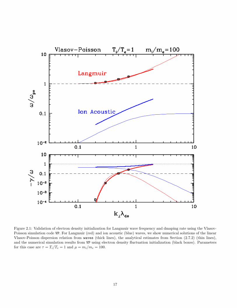
Figure 2.1: Validation of electron density initialization for Langmuir wave frequency and dmaping rate using the Vlasov-Poisson simulation code VP. For Langmuir (red) and ion acoustic (blue) waves, we show numerical solutions of the linearVlasov-Poisson dispersion relation from waves (thick lines), the analytical estimates from Section (2.7.2) (thin lines),and the numerical simulation results from VP using electron density fluctuation initialization (black boxes). Parametersfor this case are τ = Ti/Te = 1 and µ = mi/me = 100.
17
where the ion acoustic sound speed is given by
C2s =
Te
mi. (2.41)
Calculation for Distribution Eigenfunction
Beginning with the linearized 1D Vlasov Equation for electrostatic fluctuations,
∂f1s∂t
+ v∂f1s∂x
−qsms
∂φ
∂x
∂f0s∂v
= 0 (2.42)
we Fourier transform in space and time, thus assuming that the distribution function has the form
f1s(x, v, t) = f̃1s(k, v)ei(kx−ωt) (2.43)
and the electrostatic potential has the form
φ1(x, t) = φ̃1(k)ei(kx−ωt), (2.44)
and solve for f̃1s(k, v), yielding
f̃1s(k, v) = −qsms
kφ̃1
ω − kv
∂f0s∂v
(2.45)
Taking the equilibrium distribution function to be a Mawellian,
f0s =n0
(2π)1/2vtse−v2/2v2
ts (2.46)
the velocity derivative of f0s is given by
∂f0s∂v
= −v
v2tsf0s. (2.47)
Using this, we can simplify the solution for f̃1s(k, v) to
f̃1s(k, v) =
(
qsφ̃1
Ts
)
kv
ω − kvf0s (2.48)
Since the perturbed distribution function f1s(x, v, t) must be real, then the the Fourier transform of the distribution
function f̃1s(k, v) must satisfy a reality condition
f̃1s(−k, v) = f̃∗1s(k, v). (2.49)
Thus the initial condition for f1s(x, v, t) at t = 0 is given by
f1s(x, v, 0) =1
2
(
f̃1s(k, v)eikx + f̃∗
1s(k, v)e−ikx
)
= Re[
f̃1s(k, v)eikx]
(2.50)
18
Normalizaton of the Distribution Eigenfunction
Employing the code normalization outlined in Section (2.4), we obtain the following general result for the initial perturbed
distribution function f1s(x, v, 0),
(
vtsf1s(x, v, 0)
n0
)
= Re
[(
vtsf̃1s(k, v)
n0
)
eikλdex̂
]
(2.51)
where x̂ = x/λde. The normalized, Fourier transform of the distribution function is given by
(
vtsf̃1s(k, v)
n0
)
=qsqe
Te
Ts
(
qeφ̃1
Te
)
kλdev̂s
(
Ts
Te
me
ms
)1/2
(ω/ωpe)− kλdev̂s
(
Ts
Te
me
ms
)1/2
(
vtsf0sn0
)
(2.52)
where v̂s = v/vts. Using qe = −qi, τ = Ti/Te, and µ = mi/me to simplify the notation, we find the follow results for the
electrons and ions(
vtef̃1e(k, v)
n0
)
=
(
qeφ̃1
Te
)
kλdev̂e(ω/ωpe)− kλdev̂e
(
vtef0en0
)
(2.53)
(
vtif̃1i(k, v)
n0
)
= −1
τ
(
qeφ̃1
Te
)
kλdev̂i (τ/µ)1/2
(ω/ωpe)− kλdev̂i (τ/µ)1/2
(
vtif0in0
)
(2.54)
These are the normalized equations that are coded into the eigenfunction initialization in VP.
2.7.3 Localized Wavepacket
[Not yet implemented]
A simple way to implement a spatial localized wavepacket while maintaining the required net charge density of zero
is to use a perturbation that is odd about the center of the domain and window the waveform with an exponential (or
any other desired window) evenly about the center of the domain.
Doing a localized wavepacket will enable us to see a propagating wave even with a simple density perturbation
initialization (rather than having to initialize an exact linear eigenfunction).
2.8 Notes
1. Splitting the ballistic and wave terms, our initial perturbation will be all in the wave term, with δfeB(x, v, 0) = 0.
2. I need to implement collisions to keep velocity space resolved in the nonlinear simulations.
3. This numerical solver should help me to determine what nonlinear physical effects are included in the NL GK
simulations, and which are missing.
19
4. IMPORTANT NOTE: The potential is normalized by
φ̂ =qeφ
Te
and since qe < 0, this means that the normalized potential φ̂ has the opposite sign from φ, a point which could
very easily lead to confusion.
20
Chapter 3
Results for Landau Damping from VP:Nonlinear Vlasov-Poisson Simulation Code
3.1 Two Test Cases
Weakly Damped Case
It is important, for weakly damped cases to be properly modeled, that range of velocity space simulated includes the
resonant velocity, vmax > ω/k. If not, the damping is not properly resolved (in a linear run, the damping rate is too
low). Note also that, for weakly damped cases, nonlinear runs effectively have no damping at all. The reason is that
a run is weakly damped (for Langmuir waves, specifically) if the resonant velocity is far out in the tail of the electron
distribution function. Thus, it takes very little energy from the wave to flatten that part of the distibution function.
This is demonstrated in Figure 3.9 below.
For the weakly damped case, we take the following plasma and numerical parameters:
kλde = 0.2
ωr/ωpe = 1.06
γ/ωpe = −4.99× 10⁻⁵
nx nv vmax nL NL µ τ cfl Nt nt out δn nk1
128 256 8 5 T 100 1 0.25 5000 100 0.025 1
Note that this run becomes numerically unstable at t > 220, but this is much longer than we need (it is more than
30 Langmuir wave periods). Reducing cfl would delay or cure the computational instability.
This run has effectively no damping of the Langmuir wave, γ = 0, because wave-particle interactions very easily
flatten out the distribution function in the neighborhood of the resonant velocity, as demonstrated in Figure 3.9 below.
With a reduced cfl= 0.0625, the perturbed energy is conserved to about 0.4%.
21
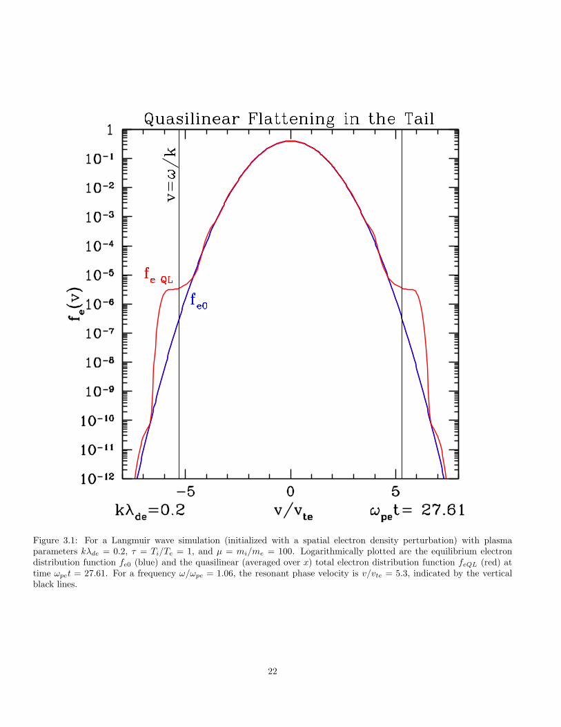
Figure 3.1: For a Langmuir wave simulation (initialized with a spatial electron density perturbation) with plasmaparameters kλde = 0.2, τ = Ti/Te = 1, and µ = mi/me = 100. Logarithmically plotted are the equilibrium electrondistribution function fe0 (blue) and the quasilinear (averaged over x) total electron distribution function feQL (red) attime ωpet = 27.61. For a frequency ω/ωpe = 1.06, the resonant phase velocity is v/vte = 5.3, indicated by the verticalblack lines.
22
Moderately Damped Case
Moderately Damped:
kλde = 0.5
ωr/ωpe = 1.43
γ/ωpe = −1.59× 10⁻¹
nx nv vmax nL NL µ τ cfl Nt nt out δn nk1
128 256 5 2 T 100 1 0.25 10000 100 0.1 1
Observations:
1. This run appears to yield a good evolution (at least up to t̂ = 49) without fe < 0 anywhere, and energy conservation
is very good.
2. No nonlinear echo behavior up to t = 49, although the exponential decay of field energy appears to be arrested
around t = 25.
3. The ballistic structure develops relatively slowly relative to the timescale of the Landau damping. In this case, the
field energy is largely completely gone by t̂ = 18.
4. The overall odd oscillation in δfew is due to the wave oscillation behavior, and varies sinusoidally in space. What
remains is the quasilinear version of the perturbation when averaged over space.
5. Note, although the δfew looks even, perhaps the field changes sign and so the signature is heating/damped is
thereby the same on both sides?
6. Question: Is a spatial average possible before computing the energy by velocity integration? If so, then the
quasilinear pieces of the distribution function tell you about the total change in the distribution function.
7. Note that δfewQL in Figure 3.8 looks exactly even in v, meaning that the energy transfer will be exactly odd as
needed (no need here to separate even and odd!).
3.2 Identification through Correlations
In this section I outline ideas on how to identify the signature of Landau damping through correlations.
1. For weakly damped runs, the normalized correlations will show a signature at the phase velocity way out in the
tail. But the unnormalized correlations will see basically nothing. For real spacecraft measurements, the small
correlated fluctuations in the tail will probably not be possible to observe (which is not a problem, since there is
little damping happening).
2. The key problem is to separate the oscillating energy transfer between particles and fields due to a wave from the
secular energy transfer due resonant wave-particle interactions. The correlations may help with this, because the
net energy transfer is a wave is zero, so if the signal is averaged over a few wave periods, the oscillating wave energy
23
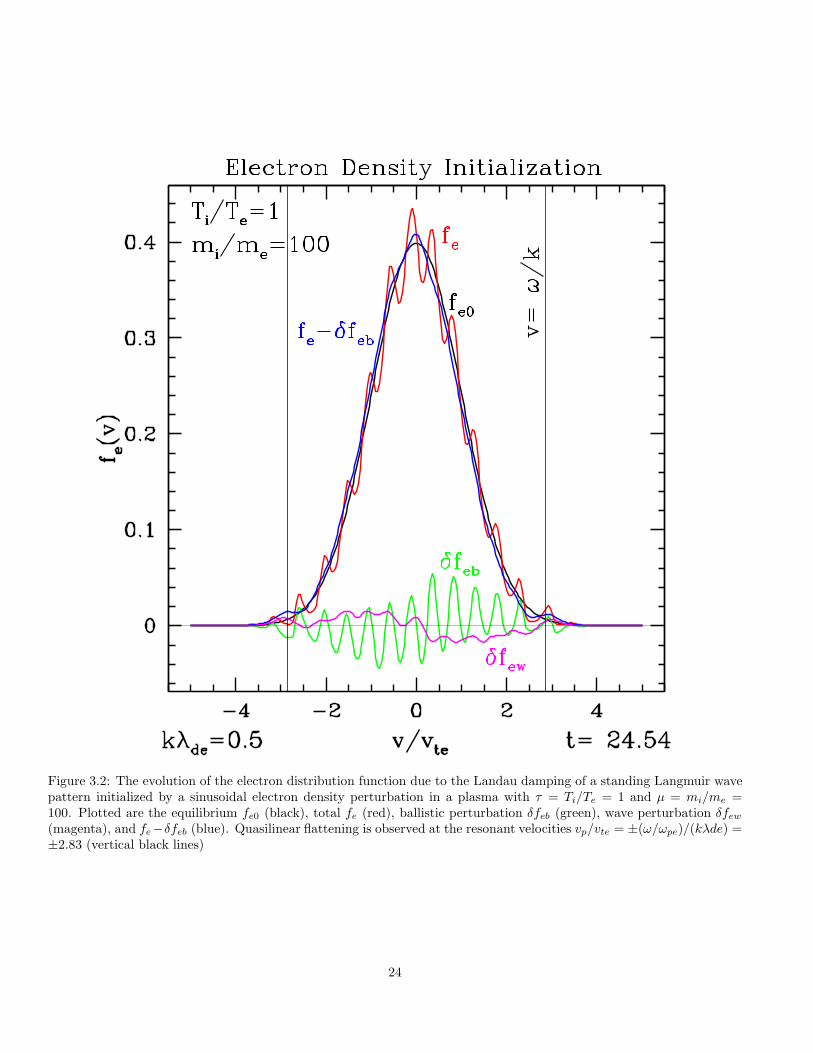
Figure 3.2: The evolution of the electron distribution function due to the Landau damping of a standing Langmuir wavepattern initialized by a sinusoidal electron density perturbation in a plasma with τ = Ti/Te = 1 and µ = mi/me =100. Plotted are the equilibrium fe0 (black), total fe (red), ballistic perturbation δfeb (green), wave perturbation δfew(magenta), and fe−δfeb (blue). Quasilinear flattening is observed at the resonant velocities vp/vte = ±(ω/ωpe)/(kλde) =±2.83 (vertical black lines)
24
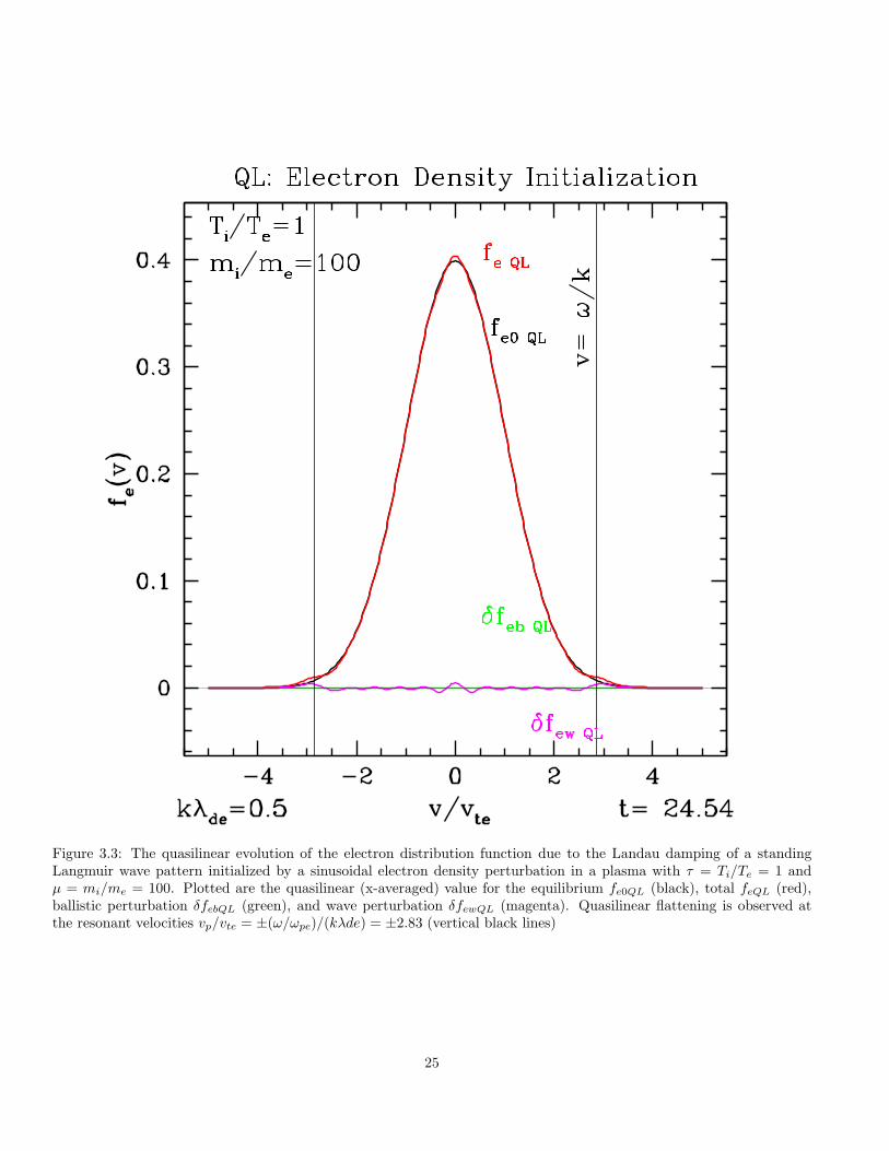
Figure 3.3: The quasilinear evolution of the electron distribution function due to the Landau damping of a standingLangmuir wave pattern initialized by a sinusoidal electron density perturbation in a plasma with τ = Ti/Te = 1 andµ = mi/me = 100. Plotted are the quasilinear (x-averaged) value for the equilibrium fe0QL (black), total feQL (red),ballistic perturbation δfebQL (green), and wave perturbation δfewQL (magenta). Quasilinear flattening is observed atthe resonant velocities vp/vte = ±(ω/ωpe)/(kλde) = ±2.83 (vertical black lines)
25

Figure 3.4: Comparison of the quasilinear evolution of the electron distribution function due to the Landau dampingof a standing Langmuir wave pattern with the electron distribution function at a particular position in space, x = 0.Plasma parameters are τ = Ti/Te = 1 and µ = mi/me = 100. Plotted are the equilibrium fe0 (black), quasilinear feQL
(red), fe(x = 0) (blue), quasilinear wave perturbation δfewQL (green), and wave perturbation δfew(x = 0) (magenta).Quasilinear flattening is observed at the resonant velocities vp/vte = ±(ω/ωpe)/(kλde) = ±2.83 (vertical black lines)
26
transfer averages out. However, the secular energy transfer due to Landau damping should add constructively.
So, even if the amplitude of the secular energy transfer due to Landau damping is very small, we may be able to
distinguish it from the oscillating wave energy transfer of much larger amplitude.
3. The phase relationship between the wave fields and wave δf may also differ from the phase relationship between
the wave fields and resonant particles. This may also turn out to be a valuable quantity to measure and plot.
For example, for a wave on a string, when the kinetic energy is maximum (when the string is straight), the restoring
force is zero. When the restoring force is maximum, the kinetic energy is zero. Thus, these two quantities should
be phase-shifted from each other by π/2. We may be able to see this if we compare the right quantities analogous
to kinetic energy and restoring force for our system.
3.3 Numerical Recurrence in Linear Run
As detailed in ?, numerical recurrence of the initial conditions can occur for linear (or nonlinear) runs due to the limited
velocity space resolution. The recurrence time is given by
Trec =2π
k∆v(3.1)
Normalized in our code units, this becomes
ωpeTrec =2π
kλde(∆v/vte)(3.2)
The velocity space resolution is given by (∆v/vte) = 2(vmax/vte)/nv, where nv is the number of uniformly space points
in velocity space between −vmax ≤ v ≤ +vmax. Thus, our condition becomes
ωpeTrec =πnv
kλde(vmax/vte)(3.3)
To reproduce this effect, we take the case:
kλde = 0.5
ωr/ωpe = 1.43
γ/ωpe = −1.59× 10⁻¹
nx nv vmax nL NL µ τ cfl Nt nt out δn nk1 ωpeTrec
64 64 5 2 T 100 1 0.5 20000 100 0.1 1 80
The effect of numerical recurrence is demonstrated in Figure 3.5, where the energy as a function of time is plotted
both linearly and logarithmically. The clear signature of recurrence at ωpet ∼ 80 is evident in the linear plot. The
logarithmic plot shows that the damping rate initially agrees with the prediction from linear theory, but there appears
to be a small amplitude recurrence effect at ωpet ∼ 40, with the much stronger numerical recurrence at ωpet ∼ 80.
The lesson here is that, to ensure that even the smaller recurrence effect at ωpet ∼ 40 is avoided, to choose a small
enough ∆v such that the recurrence time is longer than the simulation time, Trec > Tsim.
27
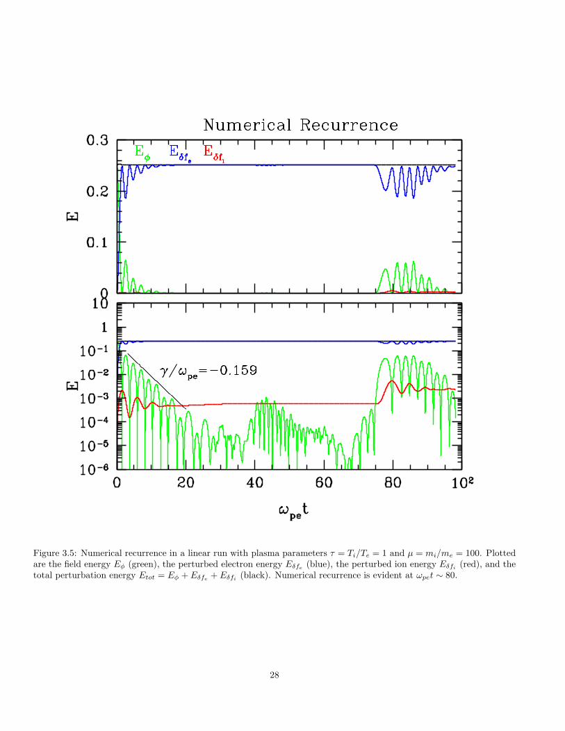
Figure 3.5: Numerical recurrence in a linear run with plasma parameters τ = Ti/Te = 1 and µ = mi/me = 100. Plottedare the field energy Eφ (green), the perturbed electron energy Eδfe (blue), the perturbed ion energy Eδfi (red), and thetotal perturbation energy Etot = Eφ + Eδfe + Eδfi (black). Numerical recurrence is evident at ωpet ∼ 80.
28
3.4 Linear Run Comments
1. In linear runs, the δfew has a constant form (odd in v) and simply decreases in amplitude over time as the electric
field damps in amplitude.
2. The initial conditions (any variation of deltaf with x) and the linear wave term deltaFewl provide the sources for
the ballistic term.
3. There is no net energy transfer into the δfs in the linear runs, because the ballistic term cannot create energy (it
just advects energy) and linear wave-particle interaction term both generates a δfew that is purely odd (and thereby
contains no net energy upon integration over v) and because it is also sinusoidal in x (and thereby integrates to
zero over the volume).
4. In a linear run, there really is no transfer of energy to the particles. Therefore, the description of energy transfer
in collisionless wave-particle interations is inherently incomplete in a linear treatment.
5. Is the damping of the field then due simply to linear phase mixing? This should be testable in linear runs to see if
the field damping rate obeys linear theory and whether it is due simply to ballistic mixing. I can artificially turn off
the linear term and see how fast the field damps in time (due strictly to ballistic term). It may be that the linear
wave-particle interactions term feeds the ballistic term in just such a way that you get the right damping rate, and
that without that term the field damps (due strictly to linear phase mixing) but at the wrong damping rate.
3.5 Nonlinear Run Comments
1. For weakly damped runs, nonlinear runs effectively have no damping at all. The reason is that, a run is weakly
damped (for Langmuir waves, specifically) if the resonant velocity is far out in the tail of the electron distribution
function. Thus, it takes very little energy from the wave to flatten that part of the distibution function.
29
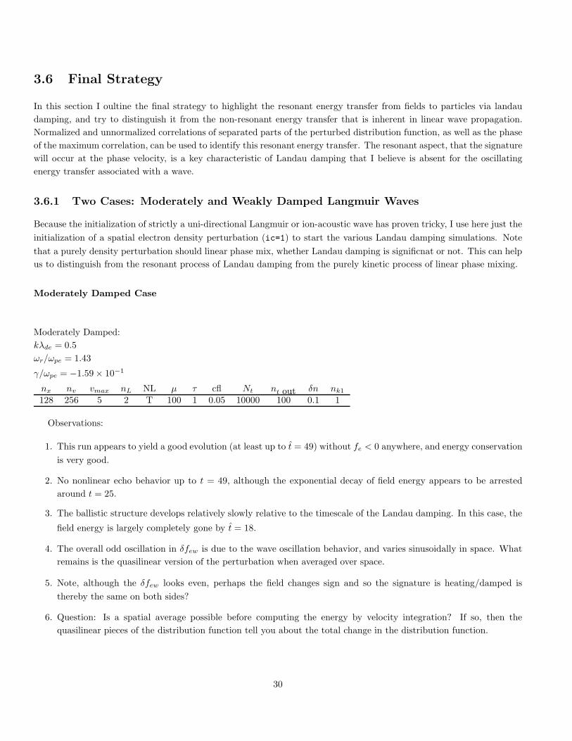
3.6 Final Strategy
In this section I oultine the final strategy to highlight the resonant energy transfer from fields to particles via landau
damping, and try to distinguish it from the non-resonant energy transfer that is inherent in linear wave propagation.
Normalized and unnormalized correlations of separated parts of the perturbed distribution function, as well as the phase
of the maximum correlation, can be used to identify this resonant energy transfer. The resonant aspect, that the signature
will occur at the phase velocity, is a key characteristic of Landau damping that I believe is absent for the oscillating
energy transfer associated with a wave.
3.6.1 Two Cases: Moderately and Weakly Damped Langmuir Waves
Because the initialization of strictly a uni-directional Langmuir or ion-acoustic wave has proven tricky, I use here just the
initialization of a spatial electron density perturbation (ic=1) to start the various Landau damping simulations. Note
that a purely density perturbation should linear phase mix, whether Landau damping is significnat or not. This can help
us to distinguish from the resonant process of Landau damping from the purely kinetic process of linear phase mixing.
Moderately Damped Case
Moderately Damped:
kλde = 0.5
ωr/ωpe = 1.43
γ/ωpe = −1.59× 10⁻¹
nx nv vmax nL NL µ τ cfl Nt nt out δn nk1
128 256 5 2 T 100 1 0.05 10000 100 0.1 1
Observations:
1. This run appears to yield a good evolution (at least up to t̂ = 49) without fe < 0 anywhere, and energy conservation
is very good.
2. No nonlinear echo behavior up to t = 49, although the exponential decay of field energy appears to be arrested
around t = 25.
3. The ballistic structure develops relatively slowly relative to the timescale of the Landau damping. In this case, the
field energy is largely completely gone by t̂ = 18.
4. The overall odd oscillation in δfew is due to the wave oscillation behavior, and varies sinusoidally in space. What
remains is the quasilinear version of the perturbation when averaged over space.
5. Note, although the δfew looks even, perhaps the field changes sign and so the signature is heating/damped is
thereby the same on both sides?
6. Question: Is a spatial average possible before computing the energy by velocity integration? If so, then the
quasilinear pieces of the distribution function tell you about the total change in the distribution function.
30
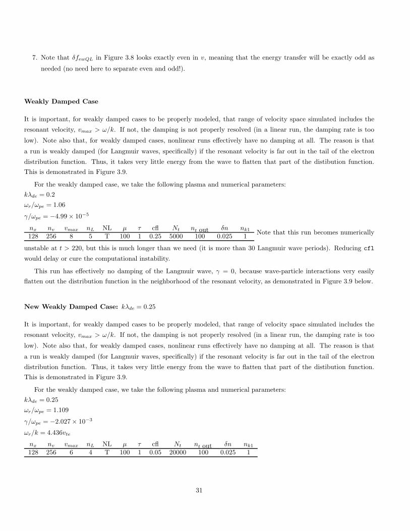
7. Note that δfewQL in Figure 3.8 looks exactly even in v, meaning that the energy transfer will be exactly odd as
needed (no need here to separate even and odd!).
Weakly Damped Case
It is important, for weakly damped cases to be properly modeled, that range of velocity space simulated includes the
resonant velocity, vmax > ω/k. If not, the damping is not properly resolved (in a linear run, the damping rate is too
low). Note also that, for weakly damped cases, nonlinear runs effectively have no damping at all. The reason is that
a run is weakly damped (for Langmuir waves, specifically) if the resonant velocity is far out in the tail of the electron
distribution function. Thus, it takes very little energy from the wave to flatten that part of the distibution function.
This is demonstrated in Figure 3.9.
For the weakly damped case, we take the following plasma and numerical parameters:
kλde = 0.2
ωr/ωpe = 1.06
γ/ωpe = −4.99× 10⁻⁵
nx nv vmax nL NL µ τ cfl Nt nt out δn nk1
128 256 8 5 T 100 1 0.25 5000 100 0.025 1Note that this run becomes numerically
unstable at t > 220, but this is much longer than we need (it is more than 30 Langmuir wave periods). Reducing cfl
would delay or cure the computational instability.
This run has effectively no damping of the Langmuir wave, γ = 0, because wave-particle interactions very easily
flatten out the distribution function in the neighborhood of the resonant velocity, as demonstrated in Figure 3.9 below.
New Weakly Damped Case: kλde = 0.25
It is important, for weakly damped cases to be properly modeled, that range of velocity space simulated includes the
resonant velocity, vmax > ω/k. If not, the damping is not properly resolved (in a linear run, the damping rate is too
low). Note also that, for weakly damped cases, nonlinear runs effectively have no damping at all. The reason is that
a run is weakly damped (for Langmuir waves, specifically) if the resonant velocity is far out in the tail of the electron
distribution function. Thus, it takes very little energy from the wave to flatten that part of the distibution function.
This is demonstrated in Figure 3.9.
For the weakly damped case, we take the following plasma and numerical parameters:
kλde = 0.25
ωr/ωpe = 1.109
γ/ωpe = −2.027× 10⁻³
ωr/k = 4.436vte
nx nv vmax nL NL µ τ cfl Nt nt out δn nk1
128 256 6 4 T 100 1 0.05 20000 100 0.025 1
31

Figure 3.6: The evolution of the electron distribution function due to the Landau damping of a standing Langmuir wavepattern initialized by a sinusoidal electron density perturbation in a plasma with τ = Ti/Te = 1 and µ = mi/me =100. Plotted are the equilibrium fe0 (black), total fe (red), ballistic perturbation δfeb (green), wave perturbation δfew(magenta), and fe−δfeb (blue). Quasilinear flattening is observed at the resonant velocities vp/vte = ±(ω/ωpe)/(kλde) =±2.83 (vertical black lines)
32

Figure 3.7: The quasilinear evolution of the electron distribution function due to the Landau damping of a standingLangmuir wave pattern initialized by a sinusoidal electron density perturbation in a plasma with τ = Ti/Te = 1 andµ = mi/me = 100. Plotted are the quasilinear (x-averaged) value for the equilibrium fe0QL (black), total feQL (red),ballistic perturbation δfebQL (green), and wave perturbation δfewQL (magenta). Quasilinear flattening is observed atthe resonant velocities vp/vte = ±(ω/ωpe)/(kλde) = ±2.83 (vertical black lines)
33
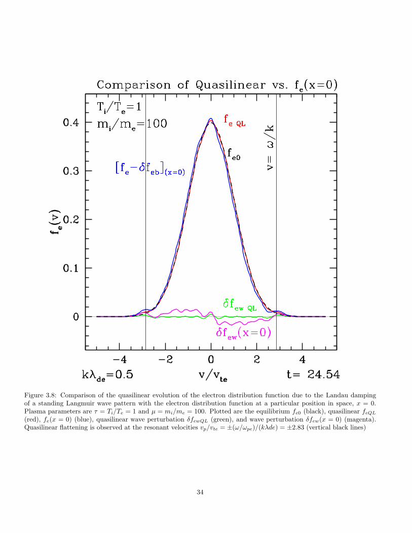
Figure 3.8: Comparison of the quasilinear evolution of the electron distribution function due to the Landau dampingof a standing Langmuir wave pattern with the electron distribution function at a particular position in space, x = 0.Plasma parameters are τ = Ti/Te = 1 and µ = mi/me = 100. Plotted are the equilibrium fe0 (black), quasilinear feQL
(red), fe(x = 0) (blue), quasilinear wave perturbation δfewQL (green), and wave perturbation δfew(x = 0) (magenta).Quasilinear flattening is observed at the resonant velocities vp/vte = ±(ω/ωpe)/(kλde) = ±2.83 (vertical black lines)
34

Figure 3.9: For a Langmuir wave simulation (initialized with a spatial electron density perturbation) with plasmaparameters kλde = 0.2, τ = Ti/Te = 1, and µ = mi/me = 100. Logarithmically plotted are the equilibrium electrondistribution function fe0 (blue) and the quasilinear (averaged over x) total electron distribution function feQL (red) attime ωpet = 27.61. For a frequency ω/ωpe = 1.06, the resonant phase velocity is v/vte = 5.3, indicated by the verticalblack lines.
35
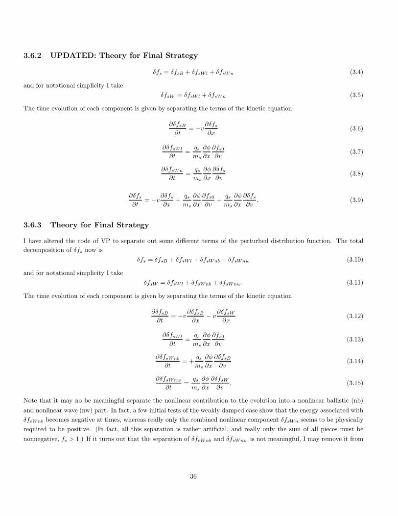
3.6.2 UPDATED: Theory for Final Strategy
δfs = δfsB + δfsWl + δfsWn (3.4)
and for notational simplicity I take
δfsW = δfsWl + δfsWn (3.5)
The time evolution of each component is given by separating the terms of the kinetic equation
∂δfsB∂t
= −v∂δfs∂x
(3.6)
∂δfsWl
∂t=
qsms
∂φ
∂x
∂fs0∂v
(3.7)
∂δfsWn
∂t=
qsms
∂φ
∂x
∂δfs∂v
(3.8)
∂δfs∂t
= −v∂δfs∂x
+qsms
∂φ
∂x
∂fs0∂v
+qsms
∂φ
∂x
∂δfs∂v
, (3.9)
3.6.3 Theory for Final Strategy
I have altered the code of VP to separate out some different terms of the perturbed distribution function. The total
decomposition of δfs now is
δfs = δfsB + δfsWl + δfsWnb + δfsWnw (3.10)
and for notational simplicity I take
δfsW = δfsWl + δfsWnb + δfsWnw. (3.11)
The time evolution of each component is given by separating the terms of the kinetic equation
∂δfsB∂t
= −v∂δfsB∂x
− v∂δfsW∂x
(3.12)
∂δfsWl
∂t=
qsms
∂φ
∂x
∂fs0∂v
(3.13)
∂δfsWnb
∂t= +
qsms
∂φ
∂x
∂δfsB∂v
(3.14)
∂δfsWnw
∂t=
qsms
∂φ
∂x
∂δfsW∂v
. (3.15)
Note that it may no be meaningful separate the nonlinear contribution to the evolution into a nonlinear ballistic (nb)
and nonlinear wave (nw) part. In fact, a few initial tests of the weakly damped case show that the energy associated with
δfeWnb becomes negative at times, whereas really only the combined nonlinear component δfsWn seems to be physically
required to be positive. (In fact, all this separation is rather artificial, and really only the sum of all pieces must be
nonnegative, fs > 1.) If it turns out that the separation of δfeWnb and δfsWnw is not meaningful, I may remove it from
36
the code (because it does slow down the code). However, if there is any simplification, this separation may yield further
insight.
Energetic arguments help us to identify which components of the perturbed distribution function are associated with
the change in the energy of the particles (due to Landau damping). Although a general case (spacecraft measurements or
nonlinear gyrokinetic simulations) cannot separate out the different constributions δfs = δfsB+δfsWl+δfsWnb+δfsWnw,
we hope to identify of strategy of correlation measurements that can highlight this signature without the separation of
these different contributions to δfs. Here I outline the simple arguments about energy conservation (some repitition from
the Theory section).
The conserved Vlasov-Poisson energy is given by
W =
∫
d3x|E|2
8π+∑
s
∫
d3x
∫
dv1
2msv
2fs. (3.16)
Taking the time derivative of this conserved energy, we find that the energy gain by the particles must be equal to the
energy lost from the electrostatic field,
∂
∂t
∑
s
∫
d3x
∫
dv1
2msv
2fs = −∂Wφ
∂t(3.17)
Therefore, the rate of energy exchange (gain or loss) for a species s is given by
∂Ws
∂t=
∂
∂t
∫
d3x
∫
dv1
2msv
2fs =
∫
d3x
∫
dv1
2msv
2 ∂fs∂t
(3.18)
We focus here on the energy gain by species s, with the assumption that the total distribution function is given by
fs(x, v, t) = fs0(v) + δfs(x, v, t), (3.19)
where the equilibirum distribution function is assumed to be uniform in space and static in time. We also make the
additional assumption that fs0(v) is an even function of velocity, but it need not be a Maxwellian.
By substituting into (3.18) for ∂fs∂t from the kinetic equation with the different contributions of the perturbed distri-
bution function in (3.10) separated out, we obtain
∂Ws
∂t=
∫
d3x
∫
dv1
2msv
2 ∂fs∂t
=
∫
d3x
∫
dv1
2msv
2
[
−v∂δfs∂x
+qsms
∂φ
∂x
∂fs0∂v
+qsms
∂φ
∂x
∂δfsB∂v
+qsms
∂φ
∂x
∂δfsW∂v
]
(3.20)
In this equation, only the last two terms contribute to a non-zero change in the particle energy (after integrating over
velocity space and space).
The first term, the ballistic term, can expressed as a perfect differential in x,
∫
dx
∫
dv1
2msv
2
[
−v∂δfs∂x
]
=
∫
dx∂
∂x
[∫
dv1
2msv
2δfs
]
= 0 (3.21)
so for periodic or infinite boundaries yields a zero value.
37
The second term may be written
∫
dx
∫
dv1
2msv
2
[
qsms
∂φ
∂x
∂fs0∂v
]
=
∫
dxqs2
∂φ
∂x
[∫
dv v2∂fs0∂v
]
=
∫
dx∂
∂x
{
qsφ
2
[∫
dv v2∂fs0∂v
]}
= 0. (3.22)
Since we have chosen fs0 to be an even function of v, then its derivative ∂fs0/∂v is an odd function, so the integrand of
the velocity integral becomes an odd function evaluated over an even interval, yielding zero. Another way to see this is
to replace evaluate the derivative as ∂fs0/∂v = −(v/v2ts)fs0, leading to a velocity integral
−
∫ ∞
−∞
dvv3
v2tsfs0 = 0. (3.23)
since, with fs0 even, the integrand is once again odd. In addition, because fs0 is not a function of x, everything in the
curly braces is also a perfect differential, so this term also vanishes over integration over all space.
This leaves the last two terms as the only ones possibly responsible for the resonant energy transfer in Landau damping.
Note that, we can also separate the energy associated with these two components (not taking the time derivative of Ws),
to yield
Ws =∂
∂t
∑
s
∫
d3x
∫
dv1
2msv
2(δfsWnb + δfsWnw) (3.24)
Since the velocity integral is nonzero only for the even components of δfsWnb and δfsWnw, visual inspection of these
components can help us see the signature of Landau damping in velocity space. Note, however, that I do not think we
should actually take just the even component—our diagnostics should be able to distinguish this without separating odd
and even components.
3.6.4 Results for Weakly Damped Case
First, we plot the different components of the perturbed electron distribution function for the weakly damped case.
Plotted in Figure 3.11 are the components of the perturbed electron distribution function. Note that the two components
that lead to a secular transfer of energy, δfsWnb (red) and δfsWnw, are the smallest contributions. Thus, it will be
necessary to separate this smaller signal from the larger signals.
Next, we plot the quasilinear (x-averaged) distribution function components at the same time with sufficient zoom
to see that structure at the resonant phase velocity. Note that, in this plot, you can see in the δfsWnb component (red)
the resonant signature of flattening of the distribution function. In this weakly damped case, there is very little energy
transfer, but nonetheless this is the signature of the quasilinear evolution due to Landau damping way out in the tail of
the distribution function.
What we want to do is perform correlations of the electric field with the different components δfsj of the distributin
function (where j stands for any of the different components), C(E, qsvδfsj). Looking at both the normalized and
unnormalized correlation, as well as the phase of the maximum correlation, will hopefully enable us to see that resonant
effect (even in this very weakly damped case, which is probably unobservable in nonlinear GK simulations and spacecraft
measurements). Note, we should do correlations with the following δfsj :
1. δfsB
38
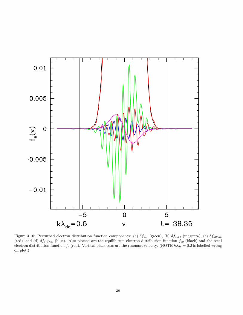
Figure 3.10: Perturbed electron distribution function components: (a) δfsB (green), (b) δfsWl (magenta), (c) δfsWnb
(red) ,and (d) δfsWnw (blue). Also plotted are the equilibirum electron distribution function fe0 (black) and the totalelectron distribution function fe (red). Vertical black bars are the resonant velocity. (NOTE kλde = 0.2 is labelled wrongon plot.)
39
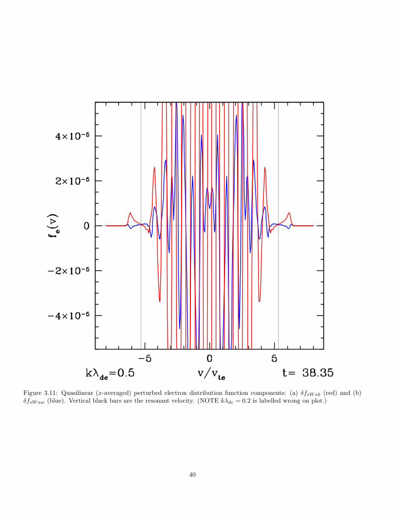
Figure 3.11: Quasilinear (x-averaged) perturbed electron distribution function components: (a) δfsWnb (red) and (b)δfsWnw (blue). Vertical black bars are the resonant velocity. (NOTE kλde = 0.2 is labelled wrong on plot.)
40
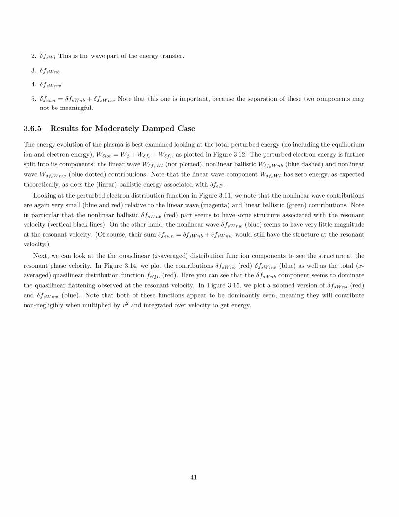
2. δfsWl This is the wave part of the energy transfer.
3. δfsWnb
4. δfsWnw
5. δfewn = δfsWnb + δfsWnw Note that this one is important, because the separation of these two components may
not be meaningful.
3.6.5 Results for Moderately Damped Case
The energy evolution of the plasma is best examined looking at the total perturbed energy (no including the equilibrium
ion and electron energy), Wδtot = Wφ +Wδfe +Wδfi , as plotted in Figure 3.12. The perturbed electron energy is further
split into its components: the linear wave WδfeWl (not plotted), nonlinear ballistic WδfeWnb (blue dashed) and nonlinear
wave WδfeWnw (blue dotted) contributions. Note that the linear wave component WδfeWl has zero energy, as expected
theoretically, as does the (linear) ballistic energy associated with δfeB.
Looking at the perturbed electron distribution function in Figure 3.11, we note that the nonlinear wave contributions
are again very small (blue and red) relative to the linear wave (magenta) and linear ballistic (green) contributions. Note
in particular that the nonlinear ballistic δfsWnb (red) part seems to have some structure associated with the resonant
velocity (vertical black lines). On the other hand, the nonlinear wave δfsWnw (blue) seems to have very little magnitude
at the resonant velocity. (Of course, their sum δfewn = δfsWnb + δfsWnw would still have the structure at the resonant
velocity.)
Next, we can look at the the quasilinear (x-averaged) distribution function components to see the structure at the
resonant phase velocity. In Figure 3.14, we plot the contributions δfsWnb (red) δfsWnw (blue) as well as the total (x-
averaged) quasilinear distribution function feQL (red). Here you can see that the δfsWnb component seems to dominate
the quasilinear flattening observed at the resonant velocity. In Figure 3.15, we plot a zoomed version of δfsWnb (red)
and δfsWnw (blue). Note that both of these functions appear to be dominantly even, meaning they will contribute
non-negligibly when multiplied by v2 and integrated over velocity to get energy.
41
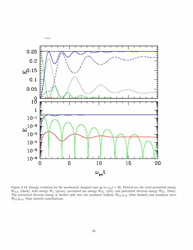
Figure 3.12: Energy evolution for the moderately damped case up to ωpet = 20. Plotted are the total perturbed energyWδtot (black), field energy Wφ (green), perturbed ion energy Wδfi (red), and perturbed electron energy Wδfe (blue).The perturbed electron energy is further split into the nonlinear ballistic WδfeWnb (blue dashed) and nonlinear waveWδfeWnw (blue dotted) contributions.
42
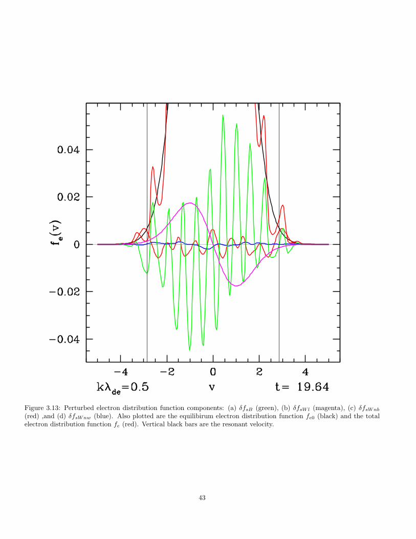
Figure 3.13: Perturbed electron distribution function components: (a) δfsB (green), (b) δfsWl (magenta), (c) δfsWnb
(red) ,and (d) δfsWnw (blue). Also plotted are the equilibirum electron distribution function fe0 (black) and the totalelectron distribution function fe (red). Vertical black bars are the resonant velocity.
43
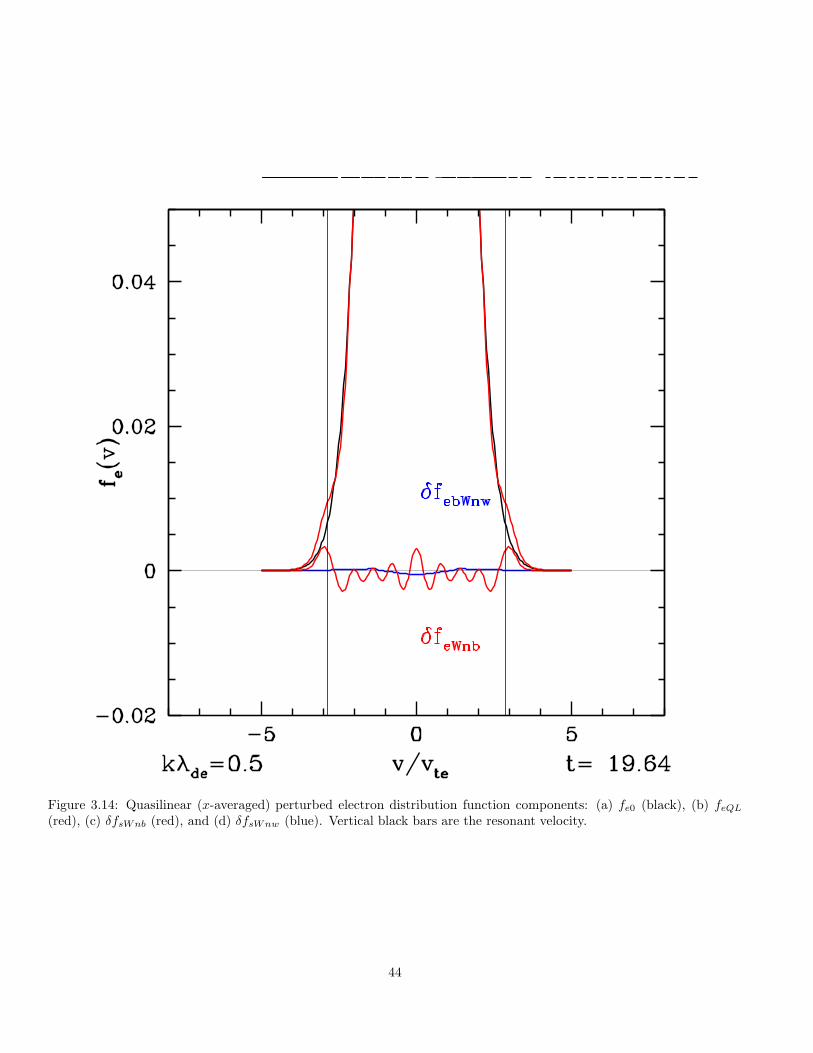
Figure 3.14: Quasilinear (x-averaged) perturbed electron distribution function components: (a) fe0 (black), (b) feQL
(red), (c) δfsWnb (red), and (d) δfsWnw (blue). Vertical black bars are the resonant velocity.
44
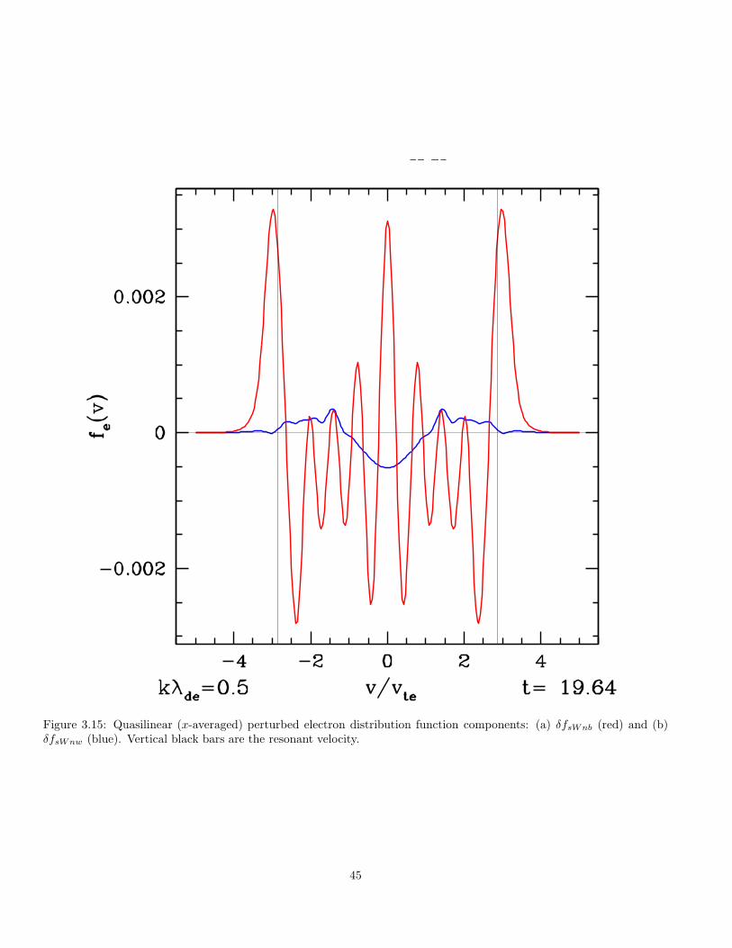
Figure 3.15: Quasilinear (x-averaged) perturbed electron distribution function components: (a) δfsWnb (red) and (b)δfsWnw (blue). Vertical black bars are the resonant velocity.
45
3.6.6 Work to do with Correlations
What we want to do is perform correlations of the electric field with the different components δfsj of the distributin
function (where j stands for any of the different components), C(E, qsvδfsj). Looking at both the normalized and
unnormalized correlation, as well as the phase of the maximum correlation, will hopefully enable us to see that resonant
effect (even in this very weakly damped case, which is probably unobservable in nonlinear GK simulations and spacecraft
measurements). Note, we should do correlations with the following δfsj :
1. δfsB
2. δfsWl This is the wave part of the energy transfer.
3. δfsWnb
4. δfsWnw
5. δfewn = δfsWnb + δfsWnw Note that this one is important, because the separation of these two components may
not be meaningful.
Note that the results above suggest that the correlation of C(E, qsvδfeWnb) should produce a significant signature
at the resonant velocity for the moderately damped case. The normalized signature should be a shift from positive to
negative correlation at v = ω/k, and the unnormalized signature should have a peak in the amplitude of the product of
these two tersm around this resonant velocity. There may also be a difference in the the correlated phase (with electric
field) of the linear wave component δfsWl relative to the nonlinear wave ballistic component δfsWnb (or the sum of the
nonlinear components, δfewn = δfsWnb + δfsWnw ).
46
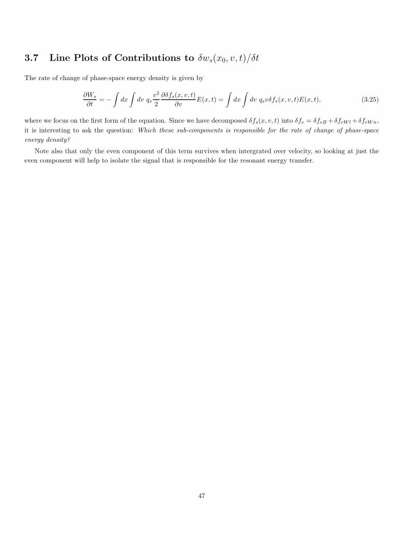
3.7 Line Plots of Contributions to δws(x0, v, t)/δt
The rate of change of phase-space energy density is given by
∂Ws
∂t= −
∫
dx
∫
dv qsv2
2
∂δfs(x, v, t)
∂vE(x, t) =
∫
dx
∫
dv qsvδfs(x, v, t)E(x, t), (3.25)
where we focus on the first form of the equation. Since we have decomposed δfs(x, v, t) into δfe = δfeB + δfeWl+ δfeWn,
it is interesting to ask the question: Which these sub-components is responsible for the rate of change of phase-space
energy density?
Note also that only the even component of this term survives when intergrated over velocity, so looking at just the
even component will help to isolate the signal that is responsible for the resonant energy transfer.
47
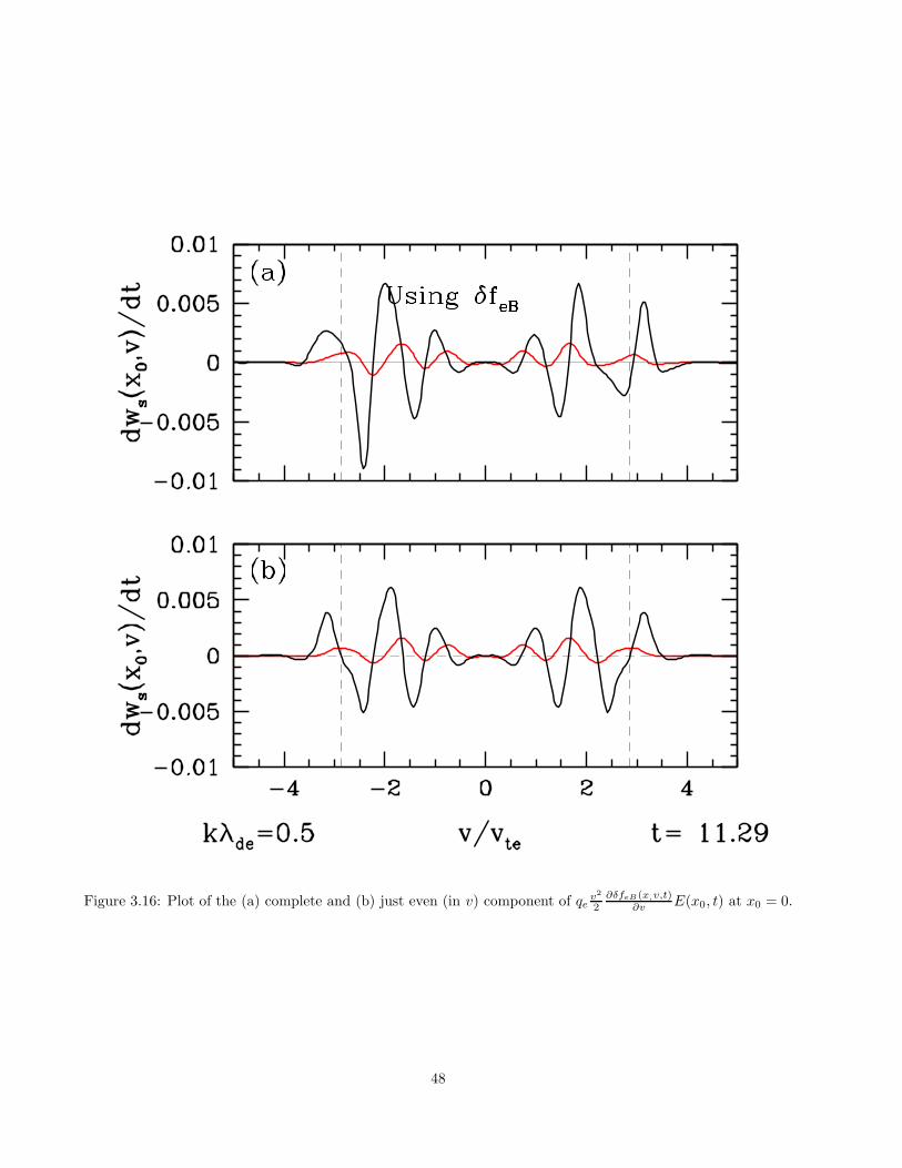
Figure 3.16: Plot of the (a) complete and (b) just even (in v) component of qev2
2∂δfeB(x,v,t)
∂v E(x0, t) at x0 = 0.
48
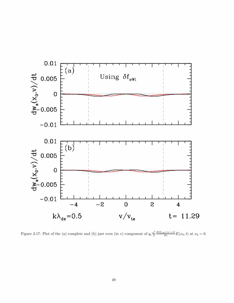
Figure 3.17: Plot of the (a) complete and (b) just even (in v) component of qev2
2∂δfeWl(x,v,t)
∂v E(x0, t) at x0 = 0.
49
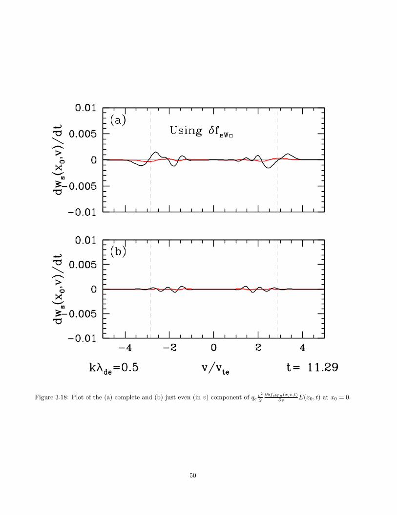
Figure 3.18: Plot of the (a) complete and (b) just even (in v) component of qev2
2∂δfeWn(x,v,t)
∂v E(x0, t) at x0 = 0.
50
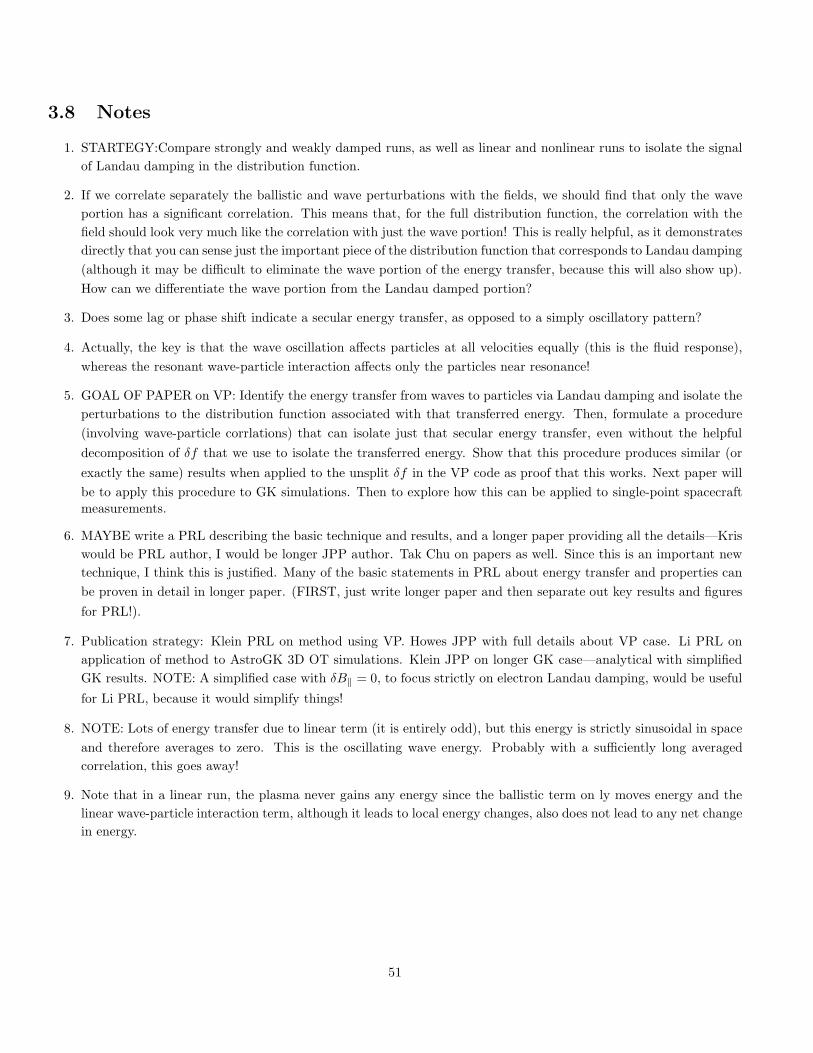
3.8 Notes
1. STARTEGY:Compare strongly and weakly damped runs, as well as linear and nonlinear runs to isolate the signal
of Landau damping in the distribution function.
2. If we correlate separately the ballistic and wave perturbations with the fields, we should find that only the wave
portion has a significant correlation. This means that, for the full distribution function, the correlation with the
field should look very much like the correlation with just the wave portion! This is really helpful, as it demonstrates
directly that you can sense just the important piece of the distribution function that corresponds to Landau damping
(although it may be difficult to eliminate the wave portion of the energy transfer, because this will also show up).
How can we differentiate the wave portion from the Landau damped portion?
3. Does some lag or phase shift indicate a secular energy transfer, as opposed to a simply oscillatory pattern?
4. Actually, the key is that the wave oscillation affects particles at all velocities equally (this is the fluid response),
whereas the resonant wave-particle interaction affects only the particles near resonance!
5. GOAL OF PAPER on VP: Identify the energy transfer from waves to particles via Landau damping and isolate the
perturbations to the distribution function associated with that transferred energy. Then, formulate a procedure
(involving wave-particle corrlations) that can isolate just that secular energy transfer, even without the helpful
decomposition of δf that we use to isolate the transferred energy. Show that this procedure produces similar (or
exactly the same) results when applied to the unsplit δf in the VP code as proof that this works. Next paper will
be to apply this procedure to GK simulations. Then to explore how this can be applied to single-point spacecraftmeasurements.
6. MAYBE write a PRL describing the basic technique and results, and a longer paper providing all the details—Kris
would be PRL author, I would be longer JPP author. Tak Chu on papers as well. Since this is an important new
technique, I think this is justified. Many of the basic statements in PRL about energy transfer and properties can
be proven in detail in longer paper. (FIRST, just write longer paper and then separate out key results and figures
for PRL!).
7. Publication strategy: Klein PRL on method using VP. Howes JPP with full details about VP case. Li PRL on
application of method to AstroGK 3D OT simulations. Klein JPP on longer GK case—analytical with simplified
GK results. NOTE: A simplified case with δB‖ = 0, to focus strictly on electron Landau damping, would be useful
for Li PRL, because it would simplify things!
8. NOTE: Lots of energy transfer due to linear term (it is entirely odd), but this energy is strictly sinusoidal in space
and therefore averages to zero. This is the oscillating wave energy. Probably with a sufficiently long averaged
correlation, this goes away!
9. Note that in a linear run, the plasma never gains any energy since the ballistic term on ly moves energy and the
linear wave-particle interaction term, although it leads to local energy changes, also does not lead to any net change
in energy.
51

52

Bibliography
53


![Hydrodynamic Limit for the Vlasov-Navier-Stokes Equations ...jabin/IUMJ_2508_2.pdf · derive the incompressible Euler equation from the Vlasov-Poisson system by Brenier [3], to investigate](https://img.pdfslide.us/doc/110x75/5ed42e002c6def41a927a773/hydrodynamic-limit-for-the-vlasov-navier-stokes-equations-jabiniumj25082pdf.jpg)
![€¦ · Web viewWe note that the Hilbert transform is also applied in [DeP] for a spectral theory of the linearized Vlasov-poisson equation. The Vlasov-Poisson equation (the collisionless](https://img.pdfslide.us/doc/110x75/5f0f7e6d7e708231d444709b/web-view-we-note-that-the-hilbert-transform-is-also-applied-in-dep-for-a-spectral.jpg)


![Scale Symmetry in the Universethe fractal geometry of the large scale structure, especially combining the Vlasov dynamics and the Poisson–Boltzmann–Emden equation [20] with the](https://img.pdfslide.us/doc/110x75/5f48ffa70ad3bb3a385445d8/scale-symmetry-in-the-universe-the-fractal-geometry-of-the-large-scale-structure.jpg)


![MULTISCALE SCHEMES FOR THE BGK-VLASOV-POISSON …mhvignal/... · neutrality when charge unbalances occur at the scale of the Debye length [9]. When the Debye length and the plasma](https://img.pdfslide.us/doc/110x75/607b80e93697a264963ab0ff/multiscale-schemes-for-the-bgk-vlasov-poisson-mhvignal-neutrality-when-charge.jpg)