Embed Size (px)
Citation preview
ED 069 214
.AUTHORTITLE
DOCUMENT RESUME
Thompson, Ivor William;A Method for DevelopingPrograms.
INSTITUTION Committee of PresidentsToronto.
REPORT NO CPUO-R-70-3PUB DATE Dec 70NOTE 72p.AVAILABLE FROM Secretariat of the Conmittee of Presidents, 230
Street West, Toronto 181, Ontario, Canada
BE 003 536
Lapp, Philip. A.Unit Costs in Educational
of Universities of Ontario,
p;)iis PRICEDESCRIPTORS
ABSTRACT.
Bloor
MF-$0.65 HC-$3.29*Educational Economics; Educational Finance;*Educational Programs; *Engineering Education;*Higher Educaiion; International Education; StudentCosts; *Unit Costs
This document presents an analysis of unit costs(annual cost per student) of engineering education in Ontario bydegree and year level. All ordinary operating expenditures arecovered including engineering department and faculty budgets, and alluniversity overhead accounts such as library, administration, andplant maintenance costs. (HS)
Committee of Presidents of Universities of OntarioCorn ite des Presidents d'Un iversi te de l'Ontario
A Method for Developing Unit Costsin Educational Programs
byIvor Wm. Thompson
andPhilip A. Lapp
ll S DITAR1MENI01 14E ALI H
CDUCAIION P. 1/Y1.11' ANC
E011CAIION
1141S 110(.01.11111AS III I l'110
IPA I ?Ai I1'1 AS IP U I POM
I III Pt ilSON Oil011(tAttilA ION 1)1110
INA I !NI, IT POilitt. 03 '.11 V. Olt ()PIN
Sl AllU 00 NW Nit SsAitlt
P1+CS17:l Of Oil (P Ou
.tA(,(1% POSII ON O3 11
CPUO Report No. 70-3December 1970
A METHOD FOR DEVELOPING UNIT COSTS IN EDUCATIONAL PROGRAMS
By
I. WM. THOMPSON'and P. A. LAPP
A REPORT SUBMITTED TOTHE COMMITTEE OF PRESIDENTS OF UNIVERSITIES OF ONTARIO
FOR THE STUDY' OF ENGINEERING EDUCATION IN ONTARIO 1970 -80
December, 1970
PUBLISHED RESEARCH STUDIES BY THE COMMITTEE OFPRESIDENTS OF UNIVERSITIES OF ONTARIO
RELATED TO THE STUDY OF ENGINEERING EDUCATION IN ONTARIO
(Available from the Secretariat of the Committee ofPresidents, 230 Bloor Street West, Toronto 181)
CPUO Report No. 70-1
CPUO Report No. 70-2
CPUO Report No. 70-3
"Undergraduate Engineering EnrolmentProjections for Ontario,: 1970-1980,"Philip A. Lapp. October, 1970.-
"An Anilysis of ProjectionS of theDemand for Engineers in Canada andOntario and An Inquiry into Substi-tu4on'Betweep Engineers and'rechnOlogists," M. L. Skolnik andW. F. McMullen, November, 1970.
"A Method for Developing Unit. Costsin Educational Programs," Ivor. Wm.
Thompson and Philip A. Lapp.December, 1970.
3
At the 39th meeting (June, 1968) of the Committee of Presidents
of Universities of Ontario, it was agreed that a comprehensive review
and analysis should be undertaken of the universities' plans for the
expansion of engineering facilities in the decade 1970-80. The
Committee of Ontario Deans of Engineering was invited to undertake
this review and analysis through the appointment of .a full-time
director. The study was to cover many areas of planning including
curriculum, enrolment, research, staff and continuing education.
The Research Division of the Committee of Presidents offered to
undertake several of the analytical sections of the study. One of the
major investigations involved the derivation of unit costs (annual
cost per student) by degree and year level taking into account cross-
departmental and faculty teaching and all ordinary operating expenses
including administrative overheads.
A summary description of the cost analysis is contained in
Appendix H of the main report.'` The purpose of this document is to
'provide a more detailed account of the analysis outlining the method-
ology, assumptions, procedures and data collection formats.
No actual input data or individual university results are
presented in this report; only averages and ranges for the whole
Ontario system of provincially-assisted engineering schools are
included. In order to illustrate the methodology, we have created
a model engineering faculty which is outlined in Appendix A. It
our opinion that the summary tables present results which will be
beneficial to the university system without the need for presenting
either the actual input data or the results for individual universities.
The presentation of detailed input data and resulting unit costs
could lead to erroneous, and perhaps even invidious, comparisons. As
will be described later there were several severe and limiting assumptions
required in the analyses. This is not unusual in such cost analyses at
this stage of their development, but because of these assumptions,
is
Ring of Iron, A Study of Engineering Education in Ontario, Committee of
Presidents of Universities of Ontario, December 1970
the results should be interpreted as having a 'range" of values
the range being dependent on the flexibility attached to the
assumptions.
This report is intended to be detailed ann in certain respects
it may even seem pedantic. We have attempted to discuss each step
thoroughly, even indicating several blind alleys which were pursued,
in order to clarify the reasons for several of the assumptions.
The term "cost" is used throughout the study, albeit somewhat
indiscriminately. .In the business environment cost covers all the
outlays for goods and services related to the product, excluding
profit. A mon': precise term in the university context would be
"expenditure", the amount each university spends from its income on
engineering students. In a university environment it is not truly
a cost because, given an increase in income, the universities would
distribute all of this increase to the various programs. From the
standpoint of this analysis, the word cost is adequate as perceived
internally by each university, but viewed externally, costs should
be interpreted as expenditures. All ordinary operating expenditures
were covered including engineering department and faculty budgets,
and all university "overhead" accounts (e.g. library, administration
and plant maintenance).
The report is divided into seven major sections. There is a
brief review of past methodologies, particularly the study conducted
by the Association of Universities and Colleges of Canada (AUCC) in
1967. The second section covers the data collection forms and
procedures together with the appropriate sample data for the model
faculty. The two sections which follow outline the methodology and
emphasize possible sources of error. Sections five and six contain
the results and conclusions together with the limitations. An
overview of the complete exercise is presented in section seven.
The authors hereby express their appreciation to Mr. Sheldon
Zelitt for his efforts on the detailed calculations and to Professor
Bernard Etkin, University of Toronto, for his derivation of the matrix
format in. Appendix C.
- iv -
This is a report of a background study toRing of Iron:,. A Study of lngineeringEducation in .Ontario(Toronto: Committee
of Presidents of Universities of Ontario,
1970). The views' expressed herein are'those of the.authors and do not .necessarily,represent those of the Committee of Presidents
of Universities of Ontario.
7
TABLE oy CONTENTS
Page
PREFACEiii
1, Review of Literature
2. Data Collection
3: Methodology
4. Sour'ces of Error 28
5, Derivation of Policy Variables. 30
6. Summary and Conausions 45
7. OverView 54
APPENDIX A - Basic Data Model University
APPENDIX B List of Symbols
APPENDIX C Unit Cost Analysis - Matrix Format
55
59
62
REVIEW OF LITERATURE
To date an extensive number of articles have been published
outlining methodologies for cost analyses. These range from a
simple proration of all expenditures equally over all students, to
complex distribution patterns having different allocation formulae
for each expenditure account. The most comprehensive dissertation
on the various methods used in the United States is provided by
James L. Miller:
"A different procedure is used in each of the stateswith the single exception that essentially the same costanalysis nrocedure ts employed in New Mexico and Colorado.
The differences among procedures often are substantial...individual procedures will he considered in detail."
There would be no advantage, in reviewing several methods in
detail. Instead we shall concentrate on explaining one of the more
familiar methods, termed the step-down method of cost analysis, which
.was employed by AUCC. This procedure was discussed by Leslie W. Knott
and others:3
"The cost centres (are) arranged in such order thatthe'department which, renders the greatest service toother departments in.proportion to benefits received.appears firSt in the arrangement. This would-meanthat activities representing primary cost centreswould appear last.. :As the experiditures for eachoverhead or general servicedepartMent, beginningWith the first, are allocated to all other depart-ments.which it serves,:the-costing process 'for thatcost centre is, for general purposes, consideredclosed. No further allocations are made to it.Under this system, expenditures for plant operationand maintenance, for example, might, as a firststep, be allocated to all departments. When thisprocess is completed, the plant management accountis closed; nothing is added to it or deducted fromit."
2
3
Miller, James L., State Budgeting for.Higher Education - TheUse of Formulas and Cost Analysis, Institute of Public Adminis-tration, The University of Michigan, Ann Arbor, 1964.
Knott, Leslie W. et alia, Cost Analysis for Collegiate Programsin Nursing Part I, Analysis of Elspres, National Leagueof Nursintl,. New York, 1956.
In the AUCC study all expenditures were grouped into the DBS-
CAUBO4 classifications as outlined in the Report of Financial Statistics
of Universities and. Colleges for the year 1966-67. All overhead
accounts were then allocated in a predetermined order, as outlined by
Knott, et alia, to the various cost centres. Several methods have
been advanced in the literature for allocating these various accounts.
In the AUCC study, for example, plant maintenance costs were allocated
on the basis of square foot area of usable space. Library costs were
allocated by charging expenditures for books, periodicals and process-
ing directly to departments for which the literature was purchased,
and by distributing all other expenditures on the basis of statistics
on the relevant use of the library facilities by staff and students.
One of the most difficult accounts to distribute has always
been academic expenditures. The treatment given in the AUCC study
is typical of the approach used in many cost analyses; academic
salaries are allocated to various activities such as instruction on
the basis of a time distribution analysis of each faculty member.
Invariably this approach has proven to be difficult and the results
are often unreliable.5. For these reasons, this approach was rejected.
Instead we sought to establish a methodology that would not require
such a detailed time analysis.
DBS-CAUBO - Dominion Bureau of Statistics - Canadian Association
of University Business Officers.
In one such survey known, to the authors several faculty members
were working more than 24 hours per day.
DATA COLLECTION
Data on student enrolments were extracted from submissions
provided
shown in
separate
business
by each university. ExaMples of the data tables used are
Figures 1 and la. Budgetaiy.information was provided in
subMissions by the Deans of'Engineering and the uniyersity .
officers; an example of the format used in collecting.the
financial information is presented in Figure 2.
To illustrate the methodology we have constructed a model
engineering faculty offering two undergraduate programs, civil
and mechanical engineering, and graduate programs in civil engineer-
ing. The undergraduate programs are two years in length with a
common first year; the graduate program offers master's and
doctoral degrees but they are of an unspecified length.
The engineering faculty is
Mechanical,
comv6Sad Of threeldepartments,
Civil, and Metallurgy andeviala Science. Students
in the engineering programs alao take courses froM one departinent
outside the faculty - Mathematics The. necessary data colleCtiOn
forms (Tables 1, 2 and 3 of the submissions). have been completed
for this model faculty together with the financial' data and
additional elements required to completely define the university
(Appendix A).
10
FIGURE 1
DATA TABLES
TABLE 1
UNDERGRADUATE CLASSES 19697'70
Class
No.
Class
Title
Given by
Staff of
the
Dept. of
No
of
Sections
Given to
Students
of the
Dept. of
Number
of from
De
Students
each
',artment
Total
Annual Con-
tact Hours.
per-Student
.Totai Annual
Staff Hours
.`per Section
Lect
Lab
Tut
Lect
Lab
Tut
Lect
Lab
Tut
1OOOOOO
00
OOOOOO
00000
TABLE 2
GRADUATE CLASSES 1969-70
Class
No.
Class
Title
Given by
Staff of
the
Dept. of
No
of
SectionS
Given-tO.
Students
of the
Dept. of_
Number
of. Students
from each
De artment
Total
:Annual Con7
tact Hours
per Student
Total Annual
Staff Hours
per Section
Lect
Lab
Tut.
Lect
Lab
Tut
Lect
,Lab
Tut
.. eeeeeeeeeeeeeeeeeee
,.-
eeeeeeeee
e.. eeeeeeeeeeee
4reee.reeeeee
*ay.,eeeeee
be
ea."
Enumeration corresponds to that used in the questionnaire.
FIGURE lA
DATA TABLES
TABLE
31 ENGINEERING ENROLMENTS
Program
1960-1961
FT
TOT
1968-1969
FTE
FT
Civil Engineering
Undergraduate
Yr.
.
3
_Graduate
Y .
2 3 4
Beyond
TOT
FTE
1
FT
1969-1970
TOT
FTE
TABLE
51
(LISTING OF ENGINEERING FACULTY MEMBERS)
Enumeration corresponds to that used in the questionnaire.
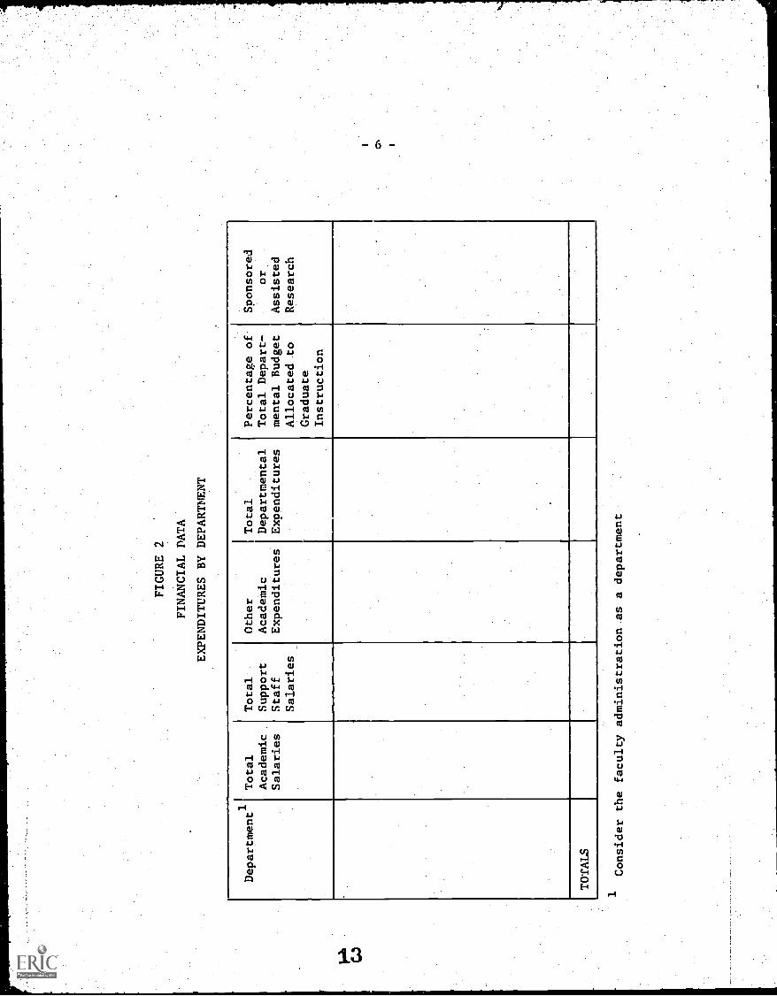
FIGURE 2
FINANCIAL DATA
EXPENDITURES BY DEPARTMENT
Department1
Total
Academic
Salaries
Total
Support
Staff
Salaries
Other
Academic
Expenditures
Total
Departmental
Expenditures
Percentage of
Total Depart-
mental Budget
Allocated to
Graduate
Instruction
Sponsored
or
Assisted
Research
I
TOTALS
1Consider the faculty administration as a department
3. METHODOLOGY
Unfortunately the entire field of education suffers from a lack
of standards and common definitions. For example, the term course
may be used to describe either a single subject or, more generally, a
group of subjects leading to a degree. Before proceeding with a
discussion of the methodology, it will be necessary to define several
of the more important terms used in the report.
In order to satisfy the requirements for a degree a student
must complete a program of study. A program then consists of a
package of courses (or classes or subjects) and/or research and/or
field work. It is important to note that students enrol in a
program of study, not a department or faculty. Faculties and
constituent departments provide services to programs in the same
manner as the library or registrar's office. Departments and
programs may carry identical titles (Department of Mechanical
Engineering compared to the degree program, Bachelor of Applied
Science - Mechanical Engineering). However, this common nomen-
clature arises because students in a program historically take the
majority of their courses from the department of the same name.
To complete a program each student must enrol in (and pass)
a specified number of courses (classes or subjects - the three terms
are used synonomously in this report). Thus a student enrolled in
an honours B.A., majoring in history, might be required to take five
history courses together with several elective courses.
In any course, the enrolment may be too large to instruct as
a single unit either for pedagogical reasons or because of available
facilities; the course may then be divided into two or more sections.
There are two methods of defining the teaching load imposed by
any course, or section of a course: one based on the student time
involved, and the other on the staff time. As an example consider
a course given by the staff of Civil Engineering in which 200
students are enrolled. The course is divided into two sections and
each section receives three hours of instruction per week. One
14
8
measure of teaching load is the number of weekly student-contact
hours (commonly abbreviated to WSCH or SCR) which is equal to the
product of the number of students enrolled and the hours per week
the course is given. In this example there are 600 weekly student-
contact hours (200 x 3). The alternate measure is the number of
weekly staff-contact hours - the time spent by the staff instructing
the course. Thus, there are 6 staff-contact hours a week (2 sections
x 3 hours per week) involved in the example course.
This concept of staff-contact hour is important because it
will be the unit introduced later for distributing academic expend-
itures. Several cost studies conducted in the past utilized
student-contact hours for this purpose. However this approach was
rejected because for obvious reasons we do not accept the premise
that a course with 40 students enrolled would cost twice as much as
the same course with 20 students. If the 40 students were sectioned
into two groups, then the staff-contact hours would double; the
workload in terms of teaching hours would double and we would then
expect the cost to increase in the same proportion.
We recognize that this approach is not entirely correct -
a true basis for distributing costs would be a combination of both
student- and staff-contact hours. Forced to elect one method, we
have chosen staff-contact hours as a better measure of cost than
student-contact hours.
The following definitions were also used in the study:
Term
Engineering facultyadministrative unit(hereafter termed
Engineering)
For programming purposes,a convenient division of theacademic year, approximatelythirteen weeks in Ontario.
- A group of resources (academic,support staff and materials)falling within an engineeringfaculty budget, under theadministrative control of a
dean or director, oftendivided into departments ordiscipline groups.
9
The first sten was to construct a "staff-contact hour matrix",
commonly referred to as a cross-over matrix, illustrating the teaching
services performed for the various programs by each department. All
teaching services provided to engineering ptograms by outside departments
and faculties were grouped into a single classification termed "other
teaching". Services provided by Engineering for non-engineering programs
were also grouped into one classification called "other Programs". Where-
ever possible, within the Engineering faculty, distinctions were maintained
between denartmentsof the faculty and also between years in a program.
in the beginning, we also-attempted to distinguish the option
streams within each program. However, as the data reduction progressed
it became obvious that this refinement would not be possible.
All computations were based on a full academic year. The total
number of yearly staff-contact hours required for each course was
computed by multiplying the annual staff hours per section by the
number of sections. The staff-contact hours required for the lecture,
laboratory and tutorial components of each course were computed
separately because the annual staff hours per section could be different
in each component (see Figure 1). Then, all staff-contact hours for a
particular course were aggregated, and prorated among all students in
the class. In the model, the course "Materials" given by the Depart-
ment of Civil Engineering (Appendix A) requires 1,200 staff-contact
hours for lectures (12 sections x 100 annual staff hours per section)
and 7,200 staff-contact hours for laboratory teaching. The 8,400 total
staff-contact hours (1,200 lecture + 7,200 laboratory) were prorated
7,000 hours (5/6) to the general first year engineering program and
1,400 hours (1/6) to the "other programs" category, i.e. to forestry
which is a non-engineering program.
The enrolment in some courses offered in Ontario followed the
pattern exhibited by the "Vibrations" course in the model; students
from two different programs were enrolled in the lecture portion of
the course but only students from one of these programs were enrolled
in the laboratory. For this case, the staff-contact hours were
computed for the lecture and laboratory component of the course but
- 10 -
not added. The lecture staff-contact hours were charged to student
enrolment in the lecture portion, and the laboratory staff-contact
hours charged to students enrolled in the laboratory part of the
course.
This proration was carried to extremes in the study. In a
class of 40 students consisting of 39 students from program A and
one student from program B, one fortieth of the staff-contact hours
would be charged to the student from program B. If this type of
analysis were repeated, we would consider it reasonable to establish
a lower bound (say 90%) such that if the percentage of students from
any one program constituted more than this lower bound, then for cost
purposes all the staff-contact hours would be charged to that program.
Students from other programs would not be assessed under these circum-
stances. If several departments taught different sections of the same
course, the relevant staff-contact hours were ascribed to the respective
department.
The staff-contact hour matrix, completed for the course "Materials",
is illustrated in Table 1, and the completed matrix for all courses is
presented in Table 2. The vertical columns list the staff-contact
hours taught by each department to each program. The horizontal rows
contain, by year in program, the number of staff-contact hours provided
by each department or group of outside faculties.
TABLE 1
STAFF-CONTACT HOUR MATRIX
("MATERIALS" COURSE ONLY)
Program Yearin
Program
Department
TotalsCivil Mechanical Metallurgyand
MaterialsScience
Other
General
Civil
Civil
Mechanical
Other
1
2
Grad.
2
-
7000
1400
7000
1400
Totals 8400 8400
TABLE 2
STAFF-CONTACT HOUR MATRIX
(ALL COURSES)
Program Yearin
Program
Department
TotalsCivil Mechanical Metallurgy.
andMaterials
Science
Other
General 1 7500 8000 - 2000 17500
Civil 2 4000 1250 3500 - 8750
Mechanical 2 - 4250 1400 5650
Civil Grad. 100 - - 100
Other 1400 500 - 1900
Totals 13000 14000 4900 2000 33900
- 12 -
In the cost study two matrices of the type illustrated in Table 2
were prepared for each university: one for all undergraduate
engineering programs,and one for all formal instruction (courses,
not research or thesis supervision) in the graduate programs.
Because there is only one graduate course in the example, graduate
nroerams have been combined with undergraduate. No distinction was made
between different levels or years in the graduate sector. Therefore
master's and doctoral candidates were considered under the single
term "graduates". Graduate thesis supervision time was treated
separately and will be discussed later.
The next stage involved the derivation of a cost per staff-
contact hour for each department or teaching unit. It is recognized
that the primary function of any academic department is to teach, and
this function has two main components: formal classroom instruction,
and research and thesis supervision, The first problem was to divide
each department or faculty budget between formal instruction (repre-
sented by staff-contact hours), and research and thesis supervision.
Normally this proration is based on a survey of the distribution of
each faculty member's time between various activities. The results
of these analyses conducted on a system basis have been unsatisfactory
and inconclusive, so in lieu of this approach a variant of a technique
used by the Committee of Vice-Chancellors and Principals in the United
Kingdom was applied.
The purpose of the work in the United Kingdom was to identify, if
possible, the objective factors influencing total departmental cost.
In all the discipline areas studies it was found that costs are a linear
function of student numbers, and no accurate separation of any research
element could be achieved.
Because of the inter-departmental loading patterns existing in
Ontario universities, it is not practical to identify each student
with a particular department. For example, in the model, how many
students should be credited to the Department of Civil Engineering?
A specific number of students cannot adequately express the teaching
load placed on the department by the various programs. Instead we
have assumed that the teaching load can be expressed by the number
of staff-contact hours, and the number of graduate students supervised.
Therefore, in the example, the teaching load for the Department of
Civil Engineering is 13,000 staff-contact hours and 100 graduate
students.
In contrast with undergraduate students each graduate was
identified with a particular department for supervision purposes.
In graduate programs, the thesis and research work is contained almost
wholly within a single department and therefore the graduate student
can be assumed to be attached to that department. Any formal or
classroom instruction in which the student is engaged will still be
credited to the department presenting the course.
The question now becomes, "how much of the departmental budget
may be ascribed to staff-contact hours, and how much to the supervision
of graduate students?". In the United Kingdom study this relationship
was assumed to be linear;, every additional undergraduate student
required "X" additional dollars, and every graduate student "Y" addit-
ional dollars. This same relationship was assumed to exist in the
engineering departments of the Ontario universities.
It was assumed that the teaching load of any department could be
expressed in terms of "teaching equivalents" where one staff-contact
hour is equal to one teaching equivalent, and one graduate student is
equal to an unknown number of teaching equivalents, "K". Then if
Ei
= number of teaching equivalents for department i
Si = number of staff-contact hours taught by department i
Gi
= number of graduates supervised by department i
E1
= Si
÷. K(Gi)
(in tne United Kingdom study, Si is replaced by the number
of undergraduate students).
20
(1)
- 14 -
A separate value of K was not determined by department.
A constant relationship was assumed for all engineering departments
in the Ontario universities. For any engineering department, the
cost of one graduate student, exclusive of classroom instruction,
was assumed to be K times the cost of one staff - contact hour. If
B. = budget of department i
a.1
= cost per teaching equivalent in department i,
and c. = constant1
then B.1
= c.1
+ a.1
(E.)1
c.1
+ a.1
(Si) + a.K (C.)1 1
Before proceeding to a discussion of how a value for K was
derived, a few comments should be directed to the financial inform-
ation which was collected. Each year the Ontario universities
submit to the Department of University Affairs (Government of the
Province of Ontario) a statement of expenditures, by major classifi-
cation, for the past year and budget estimates for the forthcoming
year. For the 1969-70 session, the Department of University Affairs
used a classification scheme which had been proposed by the Canadian
Association of University Business Officers (CAUBO) and which con-.
tained the following categories:
1. Academic (except Library)2. Library3. Student Services4. Scholarships, Bursaries and Prizes5. Sponsored or Assisted Research6. Administration7. Plant Maintenance8. General Expenditures9. Net Deficit on Ancillary Enterprises,
The academic expenditure account was further categorized as follows:
1. Academic (except Library)
(a) Salaries
(i) Academic Staff
(ii) Supporting Staff
(b) Fringe Benefits
(c) Other Academic Expenditures
(2)
-15 -
We shall be concerned first with the academic expenditure
category. Departmental budgets are usually contained entirely
within this category. There are a few exceptions where the
departmamal budget contains allocations for central library
services, computing services and other central ancillary enter-
prises. Where this was the case, the departments were asked to
indicate these appropriations which were deducted from the depart-
mental budget for the purpose of allocating the academic expenditure
category. Thus an expenditure such as central library facilities
would have involved a double counting if the charge had not been
deleted from the departmental budget. The financial information
for the study was obtained from two sources, the Canadian Association
of University Business Officers (CAUBO) forms and the responses to
the forms presented in Figure 2.
Another problem arose because the total academic expenditure
account for each university contains more than the sum of all
faculty budgets.
administration of
to this account.
to Engineering.
Areas such as the President's Office and the
the School of Graduate Studies are often charged
Part of these expenditures should be distributed
Since data were not available on their magnitude
they have not been accounted for in the analysis. As an extreme
upper limit they should represent no more than $50 per student.
The Engineering faculty budgets consisted of the individual
departmental budgets plus the faculty office budget containing items
such as the Dean's salary and costs of the faculty administration
office. The faculty office budget was distributed among departments
on the basis of the percentage contribution of each department's
budget to the total of all departmental budgets in the faculty.
In several faculty budgets there were appropriations
neither faculty administration nor departmental budgets.
Resources" wae one example of this type of appropriation.
these cases was created separately applying the rule that where
that were
"Media
Each of
- 16 -
possible the amounts should be allocated to those units bearing the
responsibility for the costs. There are too many cases to discuss
separately in this text, and therefore one example is cited as an
illustration; i.e. special counselling service established by the
faculty as an independent unit to assist first year students in
selecting courses and adjusting to the university environment.
This appropriation would be distributed equally to all first year
engineering students.
If fringe benefits were not included in the salary figures,
universities were requested to provide either a percentage allocation
for fringe benefits, or a fixed sum that was then distributed equally
over all salaries, both academic and non-academic.
In the model, Civil Engineering has an appropriation of
$600,000, Mechanical Engineering, $400,000, Metallurgy and Materials
Science, $200,000 and the faculty administration, $300,000 for a
total faculty budget of $1,500,000 (Appendix A). The faculty
administration budget of $300,000 would be prorated one-half
(600,000/1,200,000 = 1/2) to Civil Engineering, one-third to Mech-
anical Engineering and one-sixth to Metallurgy and Materials Science.
Equation (2) can now be completed for each department.
Bi = ci + ai(Si) + aiK(Gi) (2)
Civil Engineering 750,000 = c1+ a
1(13,000) + a
1K(100) (2a)
MechanicalEngineering 500,000 = c2 + a2(14,000) (2b)
Metallurgy andMaterials Science 250,000 = c
3+ a
3( 4,900) (2c)
This system of equations cannot be solved for a unique value
of K. To estimate the value of K for the Ontario engineering schools,
a linear regression was established between teaching equivalents and
the teaching salary component of the departmental budget for the thirty-
seven different departments involved in the study. The teaching salary
component was used because it was felt that this portion was more
directly related to teaching than the total departmental budget.
- 17 -
The teaching salary component was derived from the academic
salaries category of the departmental budget. In their submissions
the universities were asked for an approximate time distribution of
Engineering faculty members. It was concluded that an average of
70 percent of a faculty member's time is devoted to teaching and
supervision, with the balance being spent on administrative duties
(15 percent), consulting (10 percent) and professional and public
service (5 percent). Therefore 70 percent of academic salaries was
used in the determination of K.
The system of equations to be solved (2a, 2b, and 2c) becomes:
280,000 = cl + b1(13,000) + b1K(100) (3a)
210,000 = c2 + b2(14,000) (3b)
105,000 = c3 + b3( 4,900) (3c)
The b 's can be considered to be the "academic salaries
component" of the teaching equivalents costs (ai's). For any
selected value of K the resulting teaching equivalents can be re
gressed with the salaries component of the departmental budget.
The system of equations in the example does not have a unique
solution (there will always be 2n + 1 unknowns for this system of
n equations) nor is this a good example to demonstrate the linear
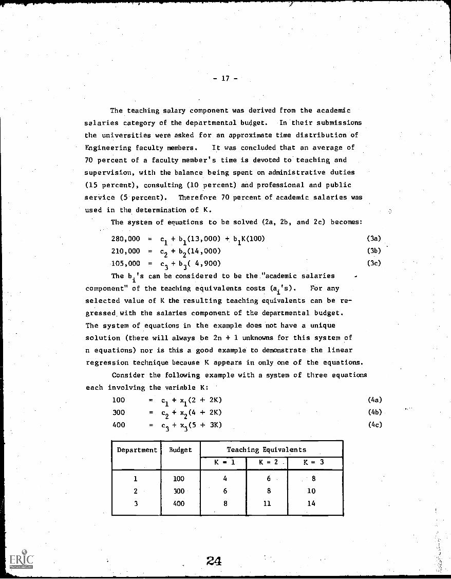
regression technique because K appears in only one of the equations.
Consider the following example with a system of three equations
each involving the variable K:
100 = c1+ x
1(2 + 2K) (4a)
300 = c2 + x2(4 + 2K) (4b)
400 = c3+ x
3(5 + 3K) (4c)
Department Budget Teaching Equivalents
K = 1 K = 2 . K = 3
1 100 4 6 8
2 300 6 8 10
3 400 8 11 14
-18-
The regression lines for K equal to one, two and three are
illustrated in Figure 3.
FIGURE 3
REGRESSION LINES TO ESTABLISH K
K=1,/ ,/,K=2
400 - /0 i'K=3
300 - w-
,e1J
oo
200 -/
100 -/
0 / *
Teaching Equivalents
The estimate of K that yielded the highest correlation coefficient
was selected as the final value. When the selected values of K were
plotted against the corresponding correlation coefficients a curve
similar to that presented in Figure 4 was derived.
1.0Max.
FIGURE 4
DETERMINATION OF K
25K
- 19 -
For the example shown in Figure 4 the value selected would
be K.. One situation that must be checked ;s the possibility of
multiple values for K, for if K. produces a maximum then perhaps
2K. or 10K. or, in the general case, nK. may also produce a maximum.
This was tested in the analysis, and when no multiple value was
found the subject wis not pursued further. (We did not consider
what course of action would have been necessary had we discovered
multiple values,)
The best linear regression yielded a correlation coefficient
of 0.98, for thirty-seven points, and a final value of K equal to
150. This corresponds to three hours per week per graduate student
for a fifty week year. In order to achieve this result it was
necessary to divide the data into two groups. When the data were
treated as a single set of thirty-seven elements, the maximum
correlation coefficient achieved was 0.93 for K equal to 180.
However, with the exception of three departments, all the depart-
ments of any one faculty were either entirely above the regression
line or entirely below. This suggested the existence of two
different "policies" or "internal weightings" for graduate students.
The data were divided into two groups (fifteen points lying above
the regression line, and twenty-two points below) and separate K
values were determined for each set. The resulting values were K
equal to 190 and 115.
Further pursuit of the two-value theorem for K would have
inferred' the recognition and assumption of two distinct policies
regarding graduate engineering studies in the Ontario universities.
Additional data such as the ratio of graduate student to total
student enrolment tends to confirm the theorem of two policies or
rather two implicit relationships. However, there was insufficiert
data to state unequivocally that these two relationships existed.
Therefore we continued to consider the data in two sets but
established a single value of K corresponding to the highest
correlation coefficient for the two sets considered together.
26
- 20
This value was 150 (staff-contact hours per student per year).
This is equivalent to saying that each graduate student requires an
average of three hours of supervision per week for a fifty week year.
The teaching load of any department can now be expressed completely
by teaching equivalents: the sum of staff-contact hours and the product
of the K factor (150) and the number of graduate students supervised in
that department. in this analysis the value of K was derived only for
the Engineering faculties and schools included in the study. The same
value is not necessarily valid for other faculties in the Ontario
universities or Engineering faculties outside the Province of Ontario.
,In using this approach we have assumed that there exists an
implicit relationship in the Ontario schools of engineering such that
the incremental cost to a department is the same whether one graduate
student is added or the teaching load is increased by 150 (the K factor)
staff-contact hours averaged, for the set of thirty-seven departments
studied.
With a value for K established, it is now possible to derive the
cost per teaching equivalent for each department. If we assume that
the same value K is applicable to the model, the system of equations
2a, 2b, and 2c can be rewritten:
750,000 - a1(13,000)+ a1(15,000) (5a)
500,000 = a2(14,000) (5b)
250,000 = a3( 4,900) (5c)
(assume c for i equal to 1,2 and 3 equal to zero, and so
attribute all costs to the teaching equivalents).
a1
$26.79
a2
$35.71
a3 = $51.02
In the model, the cost of teaching one course in civil engineering
for one hour is $26.79. Thesis supervision and research account for
54 percent (15,000/28,000) of the total departmental budget of Civil
Engineering, including faculty overheads.
- 21 -
This procedure yielded a tabulation of instruction costs per
staff-contact hour for each department within Engineering. It was
also necessary to develop the cost per staff-contact hour for
courses taught by other faculties. The first step was to derive an
average cost ner staff-contact hour for Engineering. This was derived
by dividing the total faculty budget by the total teaching equivalents
summed over all engineering departments. For the model the average
cost was $31.98 ($1,500,000/46,900 teaching equivalents).
The cost per staff-contact hour for other faculties was assumed
to be equal to the average Engineering cost ner staff-contact hour,
adjusted by the quotient of the student to staff ratio in Engineering
divided by the student to staff ratio of the whole university. The
reasoning behind this approach was that the average class size has
the greatest influence on unit costs as will be shown later, and
average class size is directly related to the student to staff ratio.
Therefore the student to staff ratios were used as a proxy measure
for comparing costs. For the model, the overall student to staff
ratio was 16:1 (10,000/625); the ratio for the Engineering faculty,
20:1 (1,000/50). Thus the cost per staff-contact hour in the other
faculties was set equal to $39.98 ($31.98 x 20/16.) (In retrospect
it could have been argued that the student to staff ratio of the
entire university should have been calculated exclusive of the
engineering students and faculty.)
Every element of the staff-contact hour matrix was multiplied
by the appropriate departmental instruction cost per staff-contact
hour to produce a cost distribution matrix (Table 3).
. 28
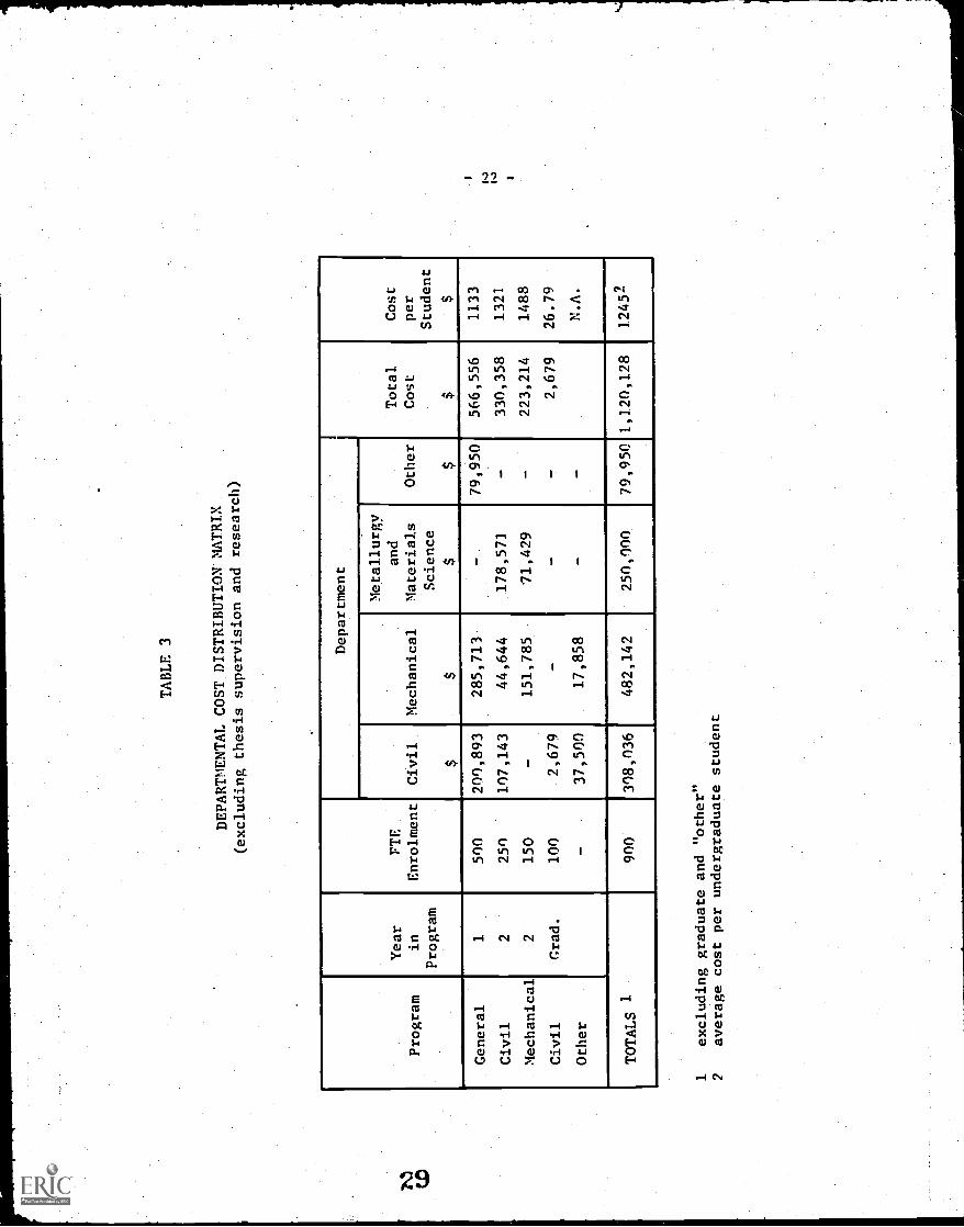
TABLE 3
DEPARTMENTAL COST DISTRIBUTION MATRIX
(excluding thesis supervision and
research)
Department
Metallurgy
Year
PTE,
and
Total
Cost
Program
in
Enrolment
Civil
Mechanical
Materials
Other
Cost
per
Program
Science
Student
$$
$$
$$
General
1500
200,893
285,713
-79,950
566,556
1133
Civil
2250
107,143
44,644
178,57]
-330,358
1321
Mechanical
2150
-151,785
'71,429
-223,214
1488
Civil
Grad.
100
2,679
--
2,679
26.79
Other
-37,500
17,858
--
N.A.
TOTALS 1
900
308,036
482,142
nomn
79,950
1,120,128
12452
excluding graduate and "other"
average cost per undergraduate student
-23-
The unit costs were computed by adding the costs along each
horizontal row, and dividing the results by the corresponding number
of full-time equivalent (FTE) students in each program and year. The
same procedure was followed for graduate programs in order to generate
the instruction portion of unit costs to which must be added the
graduate supervision costs - that portion of the total departmental
budget devoted to graduate thesis supervision and research divided by
the corresponding number of FTE graduate students. This sum yields
unit cost (excluding research grants) for each graduate program in
each university.
In the model, the total cost for the second year of the
mechanical engineering program is $223,214 distributed over 150 students
for a unit cost of $1,488. The unit cost for graduate students in civil
engineering is composed of an instructional cost per student of $26.79
($2679/100) and a thesis supervision and research cost of $4,018
($401,785/100) fora total cost of $4,045.
It was assumed that there were three components (excluding univer-
sity overhead) of total unit cost in the graduate sector: instructional
cost, thesis supervision and research, and assisted research. A compila-
tion of assisted research grants for 1969-70 was provided on a depart-
mental basis. The total departmental grant was divided by the appro-
priate number of graduate students and the result added to the other two
component costs to yield a unit cost including assisted research. (For
Engineering, assisted research money is derived principally from the
National Research Council.) The department of Civil Engineering, in
the model, received assisted research monies of $300,000. Prorated
over the graduate students in civil engineering this would raise the
cost to $7,045 ($4,045 + $300,000/100).
To this point we have discussed the distribution of two accounts:
academic expenditures and assisted research. The remaining accounts
(listed on page 14) are commonly referred to as university overhead.
The usual method of handling such accounts is to establish a distribution
formula for each one. Maintenance and physical plant, for example, may
be distributed on the basis of the percentage of floor area within the
30
-24-
jurisdiction of the unit under study. During our discussions with
the various finance officers, we could not obtain any common agreement
on methods for distributing these overhead accounts.
The only agreement we could achieve, and to which we subscribe,
was to distribute all overhead accounts equally among all students,
because of inherent limitations in the present university information
systems. c'or engineering, this would imply that the library cost per
student was equal to that for a student in the humanities or social
sciences, but the cost per student for computing services is also
considered the same for both types of students. There is a trade-off
between these accounts and it is our opinion that further accuracy
would not be achieved by introducing different distribution formulae
for each account.
Instead, the unit costs in each department were increased by a
fixed percentage derived for each university. The percentages were set
equal to the sum of academic expenditures and assisted research divided
by total ordinary operating expenditures.
Example: Let .A = academic expendituresR = assisted research0 = other expendituresT = total expendituresP = percentage to be applied for overhead
A +R + 0= TDefine: P = (A + R) /T
T = (A + R) /P
Model University:
2nd Year Civil Engineering Unit Cost = $1,321
Assisted Research = $0
Percentage(Appendix A)= 70%
Total Unit Cost = $1,887
The percentages for Ontario ranged from 55 to 75 percent depending
on the size of the institution; the average was 70 percent. The per-
centages were derived from the UA-4 reporting forms (CAUBO forms for
1969-70) submitted to the Department of University Affairs by each
university. The total unit costs for the engineering programs in
the model university are presented in Table 4.
Table 5 is a summary of average total unit costs by discipline
and year, weighted in each-case by thenumber of students for the
engineering programs in the Ontario universities. Three values are
displayed: the Ontario average, the maximum value and the minimum
value.
TABLE 4
TOTAL UNIT COSTS
.
Program
Academic Cost
Overhead
Factor
Total Unit Cost
Year
in
Program
Under-
Graduate
Graduate
(Excluding
Assisted
Research)
Graduate
(Including
Assisted
Research)
Under-
Graduate
Graduate
(Excluding
Assisted
Research)
Graduate
(Including
Assisted
Research)
General
11133
--
.7
1619
--
Civil
21321
-.7
1887
-
Mechanical
21488
.7
2126
-
Civil
Grad.
1
4045
7045
.7
-5779
10064
Average
1245
-.7
1779
--
(Excluding Graduate)
Average
(Including Graduate)
1524
1824
.7
2177
2606
- 27 -
TABLE 5
UNIT COSTS BY DISCIPLINE, YEAR AND NUMBER OF STUDENTS1969-70
PROGRAMNO. OF FTESTUDENTS
ONTARIOAVERAGE
MAXIMUM MINIMUMMAXIMUMMINIMUM
ChemicalEngineering I 444 $ 920 $ 1,740 $ 360 4.8
11 383 1,200 5,490 550 10.0111 228 2,800 4,660 990 4.7
IV 237 2,100 8,840 1,230 7.2ALL 1,292 1,550 8,840 360 24.6
Graduate - excludingassisted research ALL 320 9,190 14,730 5,760 2.6
- includingassisted research ALL 15,740 20,800 11,440 1.8
Civil 1 495 1,090 1,740 360 4.8Engineering 11 505 1,500 5,980 980 6.1
III 339 1,450 2,780 750 3.7IV 243 2,040 6,310 840 7.5
ALL 1,582 1,440 6,310 360 17.5
Graduate - excludingassisted research ALL 376 8,850 14,350 6,680 2.1
- includingassisted research ALL 14,110 23,120 9,820 2.4
Electrical I 540 1,060 1,430 360 4.0Engineering Il 560 1,010 1,500 700 2.1
111 392 1,380 4,020 1,200 3.4IV 317 1,660 4,150 890 4.7
ALL 1,809 1,220 4,150 360 11.5
Graduate - excludingassisted research ALL 413 8,150 13,700 4,370 3.1
- includingassisted research ALL 12,180 19,510 8,800 2,2
Mechanical I 529 1,050 1,430 360 4.0.
Engineering Il' 549 1,250 1,700 530 3.2
111 366 2,010 3,320 940 3.5
IV 322 1,800 6,020 1,000 6.0ALL 1,766 1,450 6,020 360 16.7
Graduate - excludingassisted research ALL 278 9,410' 15,270 6,400 2.4
- includingassisted research ALL 14,190 15,780 9,910 1.6
Metallurgical and I 61 930 1,430 360 4.0
Materials II 61 1,520 2,560 880 2.9
Engineering III 33 3,940 6,120 210 29.1
IV 38 6,850 14,460 4,470 3.2
ALL 193 2,800 14,460 210 68.9
Graduate - excludingassisted research ALL 100 10,450 17,000 7,190 2.4
- includingassisted research ALL 21,780 35,290 15,180 2.3
All Engineering 1 2,621 1,030 1,960 360 5.4
Programs II 2,450 1,270 18,760 530 35.4
III 1,709 1,850 6,120 210 29.1
IV 1,446 2,040 14,460 840 17.2
ALL 8,226 1,450 18,760 210 89.3
Graduate - excluding-assisted research ALL 2,089 8,190 17,000 4,370 3.9
.. includingassisted research ALL 10,315 13,460 35,290 8,100 4.4
-78-
4. SOURCES OF ERROR
This method of computing unit costs involved certain assumptions
whose validity is open to discussion. The most debatable assumption is
the method for prorating the departmental budget between instruction and
graduate supervision, where it was assumed that each graduate student
absorbs a fixed number of staff hours annually for graduate supervision
and research. The validity of this assumption was tested by the dispersion
of the actual departmental budgets from the values calculated using the K
factor. For the set of thirty-seven departments in Ontario, the correla-
tion coefficient was 0.98, and over 8') percent of the points fell within
an 18 percent band about the regression line. Anomalies will occur in
some departments because of the mixture of thesis and course-work master's
degree students, and variations in thesis supervision practice among
academic staff.
A second assumption used in the K value determination was the
portion of academic salaries devoted to either instruction or graduate
supervision, assumed to be 70 percent. Obviously, this will vary among
departments and individuals within a department. The figure was selected
on the basis of the submissions without a detailed time distribution study
of university staff in all of the universities.
These two assumptions were used to calculate the percentage split
of the departmental budget between instruction and graduate supervision.
In general, the calculated percentages of departmental budget devoted to
graduate instruction were slightly higher than estimated values provided
by some universities, the average difference being 8 percent.
A third assumption was the use of student to staff ratios to
compute the contact hour cost for departments outside of Engineering.
There would appear to be few alternatives until a similar cost study is
conducted for all other faculties. The student to staff ratios were
readily available though they reflect relative costs only if staff and
teaching policies are similar throughout the entire university.
A fourth assumption was the uniform division of assisted research
monies among all gradudte students within the department. The validity
of this may be questioned in specific instances, but no reasonable
alternative was apparent from available data.
-29-
The final significant assumption was the application of expen-
ditures to overhead accounts. These were applied to the unit costs
developed from the departmental budgets and included costs of library,
student services, scholarships, bursaries, administration, plant mainten-
ance, general expenditures and net deficit on ancillary enterprises, all
expressed as a percentage of the total expenditure for each university.
Errors could have been introduced in this final calculation since some of
the expenditures covered by the overhead accounts in the UA-4 forms often
are credited to the departmental budget. However, most universities did
provide data on these additional costs, including them in the departmental
budgets. In these cases, such costs were removed and were not counted
twice.
All these assumptions create possible errors in the calculations
of cost per contact hour. Errors may also be introduced in the compilation
of staff-contact hours per student where the data from the tables in
Figure 1 may contain errors and omit complete classes. If classes given
by the staff in Engineering were omitted, only the distribution of costs
among the programs would be altered, but not the average cost per engineer-
ing student.
Undergraduate thesis contact hours were not reported by all univer-
sities. For this reason, it was decided to omit these hours from the
undergraduate contact hour matrix so that undergraduate thesis costs were
distributed evenly over all teaching equivalents in Engineering. Con-
sequently, relative fourth year costs may be reduced slightly.
Omitted classes given by the faculties other than Engineering
would be excluded from the total and lost. In several cases it was found
that classes taught to graduate students by staff from other than Engineer-
ing departments were omitted, and in these cases the final unit cost
figures will be low.
-30-
5. DERIVATION OF POLICY VARIABLES
A principal purpose of the cost study was to identify
specific quantities that could be measured easily and. then used
in the establishment of administrative policies and practices.
Eight of these policy variables were identified and each can be
combined in a direct way to yield approximations to unit cost,
so that it is theoretically possible to blend each component
in an optimum fashion, consistent with fixed quality standards,
to minimize unit cost. These quantities, or policy variables,
can be derived from the unit cost computation described in
Section 3.
The administrator can develop approximate unit costs
without the necessity of completing either a detailed cost study
or an inter-departmental staff-contact hour matrix, since values
for the eight policy variables can often be determined from
available data. There are three levels of policy variables:
those that can be established at the departmental level, those
controllable at the faculty level and those that are general
university policy (several of the policy variables can be con-
trolled or established at more than one administrative level).
We shall be concerned first with identifying the policy variables
at the departmental level.
The unit cost of each undergraduate program consists of
three components: the cost attributed to the various departments
within Engineering, to other faculties, and to the overhead
accounts. We shall first introduce the policy variables that are
derived from the Engineering faculty component of unit cost.
The contribution of each department within Engineering to
the instruction cost for any year of a program can be expressed
-31-
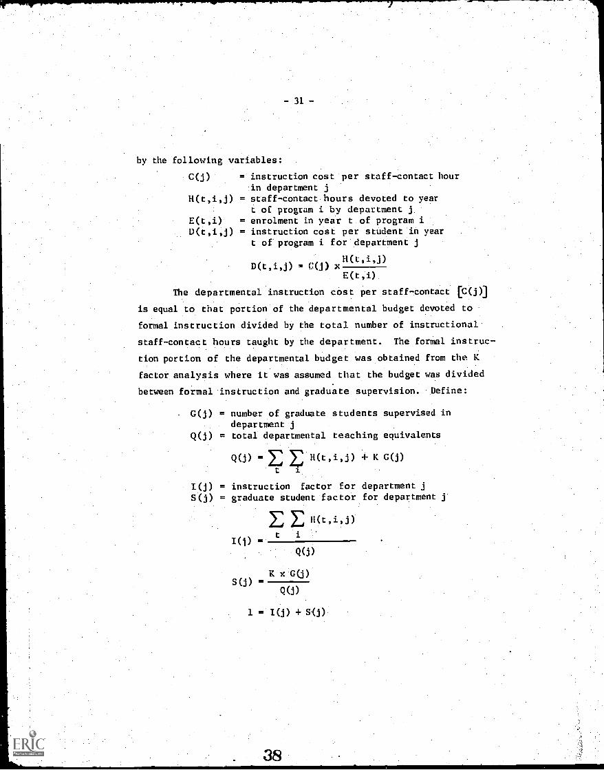
by the following variables:
C(j) = instruction cost per staff-contact hourin department j
H(t,i,j) = staff-contact hours devoted to yeart or program i by department j
E(t,i) = enrolment in year t of program iD(t,i,j) = instruction cost per student in year
t of program i for department j
D(t,i,j) = C(j) xH(t,i,j)
E(t,i)
The departmental instruction cost per staff-contact [C(j)]
is equal to that portion of the departmental budget devoted to
formal instruction divided by the total number of instructional
staff-contact hours taught by the department. The formal instruc-
tion portion of the departmental budget was obtained from the K
factor analysis where it was assumed that the budget was divided
between formal instruction and graduate supervision. Define:
G(j) = number of graduate students supervised indepartment j
Q(j) = total departmental teaching equivalents
Q(j) = H(t,i,j) + K G(j)
t i
I(j) = instruction factor for department jS(j) = graduate student factor for department j
H(t,i,j)
t i
Q(j)
K x-G(j)
4(3)
1 = I(j) + S(j)
-32-
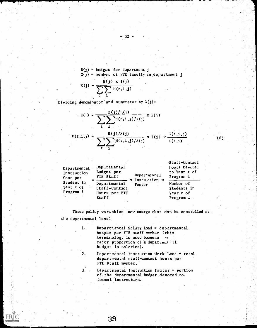
B(j) = budget for department jX(j) = number of FTE faculty in department
B(j) x 1(j)
Ey: H(t,i,j)
t i
Dividing denominator and numerator by X(j):
C(j)-
C(j) -
D(t,i,j) =
DapartmentalInstructionCost perStudent inYear t ofProgram i
B(i)P.(1)
t
3
B(j)/X(j)x I(j) k
I:22H(t,i,j)/X(j)
t i
DepartmentalBudget perFTE Staff
DepartMentalStaff7ContactHours per FTEStaff
Departmental
x Instruction xFactor
Staff-ContactHours Devotedto Year t ofProgram i
Number ofStudents inYear t ofProgram i
Three policy variables now emerge that can be controlled at
the departmental level
1. Departiv?mtal Salary Load = departmentalbudget per FTE staff member (thisterminology is used becausemajor proportion of a deparLm,:r '11budget is salaries).
2. Departmental Instruction Work Load = totaldepartmental staff-contact hours perFTE staff member.
3. Departmental Instruction Factor= portionof the departmental budget devoted toformal instruction.
(6)
-33-
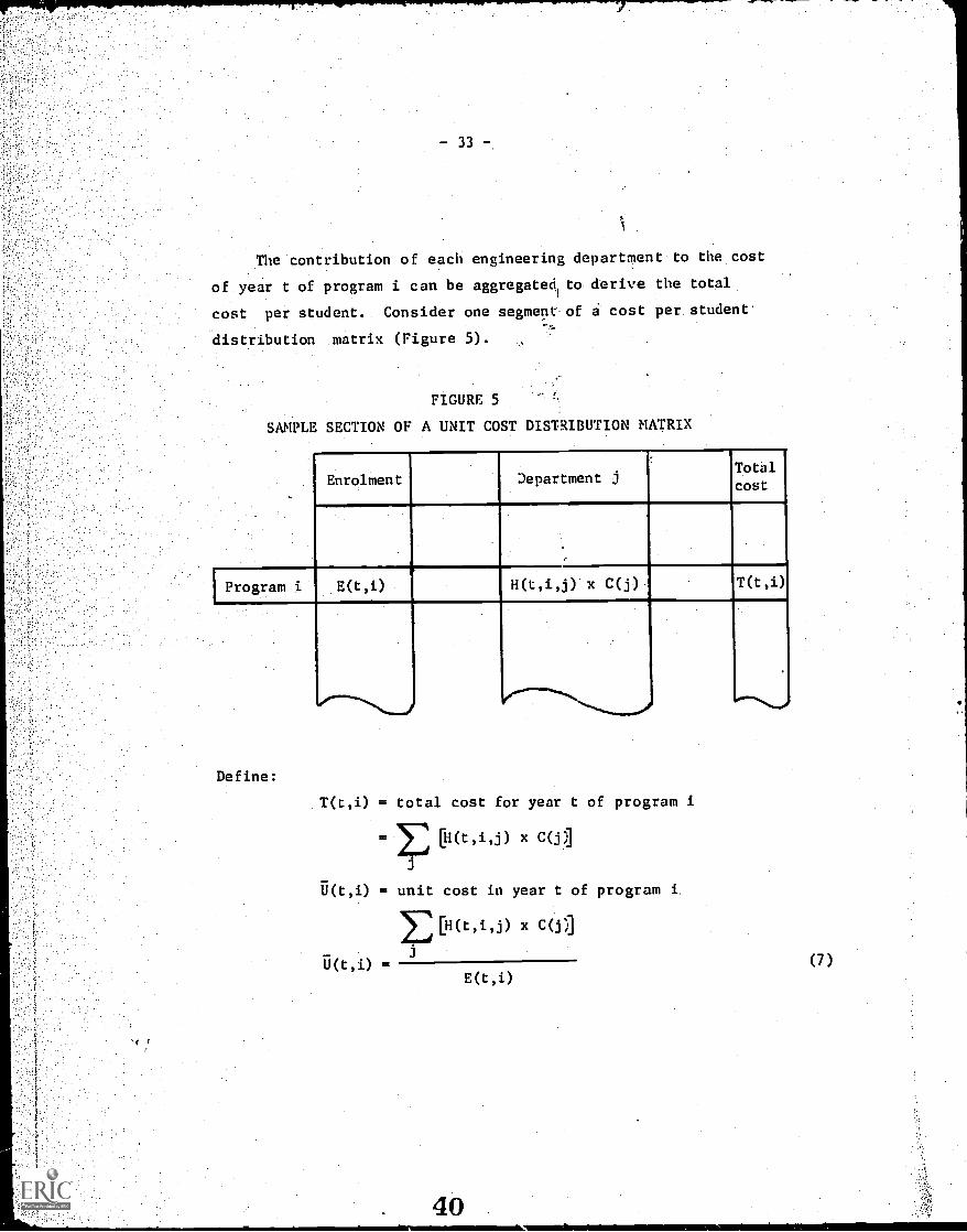
The contribution of each engineering department to the cost
of, year t of program i can be aggregatedt to derive the total
cost per student. Consider one segment of i cost per student
distribution matrix (Figure 5).
FIGURE 5
SAMPLE SECTION OF A UNIT COST DISTRIBUTION MATRIX
..
Enrolment Department jTotill.
cost
Program i E(t,i) I H(t,i,j) x C(j) T(t,i)
."---... ,
Define:
T(t,i) = total cost for year t of program i
= [H(t,i,j) x C(j1
U(t,i) = unit cost in year t of program i.
U(t,i) -
[H(t,i,j) x
E(t,i)
40.
(7)
-34-
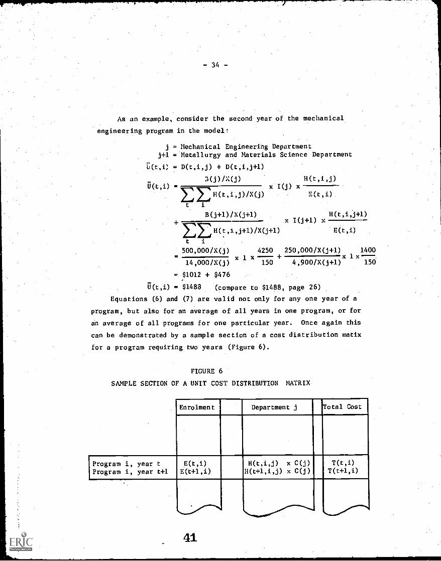
As an example, consider the second year of the mechanical
engineering program in the modell
j = Mechanical Engineering Departmentj+1 = Metallurgy and Materials Science Department
L(t,i) = D(t,i,j) + D(t,i,j+l)
3(j) /X(j) H(t,i,j)U(tii) = x I(j) x
EEH(t,i',j)/X(j) E(t,i)
t i
B(j+1)/X(j+1)I(j+1)
H(t,i,j+1)x x
2222H(t,i,j+1)/X0+1) E(t,i)
t i
500,000/X(j) 4250 250,000/X(j +1) 1400x + x 1 x
150 4,900/X(j+1) 15014,000/X(j)x 1
= $1012 + $476
U(t,i) = $1483 (compare to $1488, page 26)
Equations (6) and (7) are valid not only for any one year of a
program, but also for an average of all years in one program, or for
an average of all programs for one particular year. Once again this
can be demonstrated by a sample section of a cost distribution matix
for a program requiring two years (Figure 6).
FIGURE 6
SAMPLE SECTION OF A UNIT COST DISTRIBUTION MATRIX
Enrolment Department j Total Cost
Program i, year t E(t,i) H(t,i,j) x C(j) T(t,i)
Program i, year t+1 E(t+1,i) H(t+1,i,j) x C(j) T(t+1,i)
-35-
U(i) = unit cost in program i,
U(i)
E T(t,i) /EE(t,i)
x
t
:ES(t,i)
t.
U(t) = unit cost in year t averaged over all programs
=
U(t)
EE[H(t,i,j) x C(j)]
i j
EiE(t,i)
A cost per student averaged over all programs and all year
levels can also be derived:
= unit cost per student averaged over all programs
and all year levels
EET(t,i)/EEE(t,i)t i t
EE E[H(t,i,j) x c(j)]t i j
t
We have identified three policy variables affecting the unit
cost that are controllable at the departmental level: the average
departmental expenditure per FTE staff member, the average number
of staff-contact hours per FTE staff member and the proportion of a
department's budget that can be attributed to formal instruction.
To introduce the remaining policy variables, it will be more con-
venient to work with a unit cost averaged over all programs and
all years. The expression:
DepartmentalInstructionCost perStaff-ContactHour
or
-36-
Departmental Budgetper FTE Staff Member
Departmental Staff-Contact Hours perFTE Staff Member
Departmentalx Instruction
Factor
C(j) =B(j)/X(j) x I(j)
EEH(t,i,j)/X(j)
t i
can also be written for the faculty level:
FacultyInstructionCost perStaffContact-Hour
or
Faculty Budget perFTE Staff Member
Faculty Staff-Contact Hours perFTE Staff Member
Facultyx Instruction
Factor
j /C *= x I*
t i j /where I* = Faculty instruction factor
t i j
ESE H(t,i,j) + KE G(j)
t i j
Two additional policy variables can now be introduced:
4. Student Load = Student hours per year
-37-
5. Average Section Size = Ratio of the number ofstudents in any section to the number ofstaff teaching the section, but averagedover all sections taught by the facultyor department. For example, in a lecturesection of 100 students, the section sizewould be 100;whereas in a laboratorysection of 100 students with ten instructors,the average section size would be ten. The
average section size can be regarded asthe average student to staff ratio in allsections for any year of a program.
If:
Y(t,i,j) = yearly student hours required by year t inprogram i from department j
A* = average section size (average for the faculty)
then,
AverageSectionSize
so that
Staff-ContactHours perStudent
Average Costper Student
or
AverageCost per =Student
U
Average Yearly Class Number of
Hours per Student x Students
Total Staff-Contact Hours
Average Yearly ClassHours per Student
Average Section Size
EEEy(t,i,J) EE ,E(t i)
t i j t i
A*
Average Faculty Instruction Staff-Contact HoursCost per Staff-Contact Hour per Student
Faculty Salary Faculty Instruction StudentLoad Factor Load
Faculty Work Average SectionLoad Size
DovEx(i)= x Ii,E E Z H(t,i,j)/Ex(J)
t 1 jj
EEEEY(t,i,J1EZ E(t,i)i j
x t 1A*
44
-38-
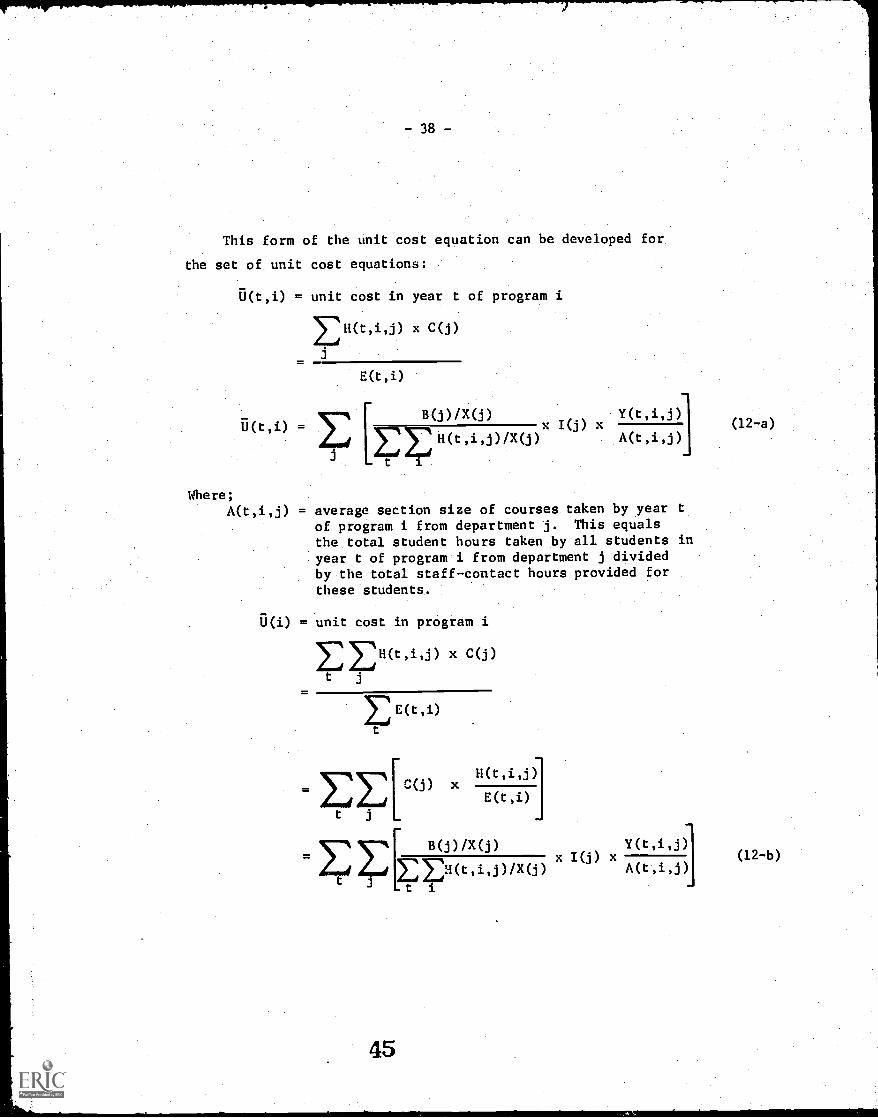
This form of the unit cost equation can be developed for
the set of unit cost equations:
= unit cost in year t of program i
x C(j)
U(t,i) =
Where;
E(t,i)
[
B(j)/X(j) Y(t,i,j)x I(j) x
2:::E H(t,i,J)/X(J) A(t,i,j)
t
A(t,i,j) = average section size of courses taken by year tof program i from department j. This equalsthe total student hours taken by all students inyear t of program i from department j dividedby the total staff-contact hours provided forthese students.
U(i) = unit cost in program i
x C(j)
t j
=EE[t j
c(J) x
.EE[ B(j) /Y(j)
tt
Y(t,i,j)x I(j) x
A(t,i,j)
(12-a)
(12 -b)
11"-
- 39 -
U(t) = unit cost in year t
x C(j)]
EE(t,i)
H(t,i,J)
E(t,i)
[.E E c(J) x
i i
[
B(j)/X(j) x I(j) xY(t
'
i'
j)12-c
EEH(t,i,J)/X(j) A(t,i,j)
t i
The average section size A(t,i,j) is a very difficult factor
to measure because it is necessary to know how many hours of
instruction each student takes from each department. Instead a
proxy measure can be introduced, A(t,i), which is an average
section size for all departments.
A(t,i,j) = Y(t,i,j)/H(t,i,j)
A(t,i) = Ey(t,i,j)/EH(t,i,j)
This expression for average section size can be substituted
into Equations 12-a, 12-b, and 12-c.
B(J)/x(i)= 1
. A(t,i) EEH(t,i,j)/X(j)t i
1B(j)/X(j)
A(t,i) Et J
t
x I(j) x Y(t,i,j) 13-a
1B(j) /X(j)
ii
E E(t)
j t
x 1(j) x Y(t,i,i) 13-b
Ix I(j) x Y(t,i,j) 13-c
-40-
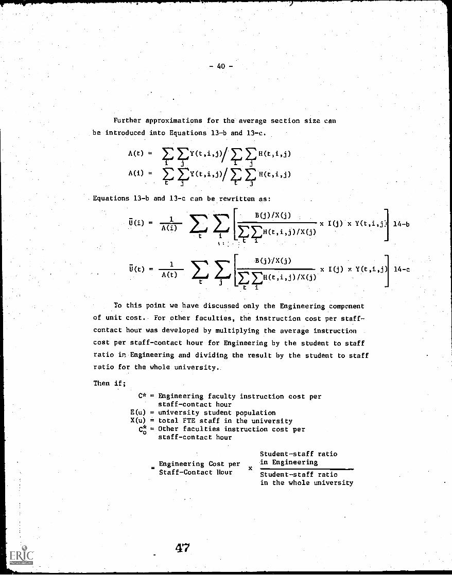
Further approximations for the average section size can
be introduced into Equations 13-b and 13-c.
A(t) = EY(t,i,j)/EFI(t, ,j)
A(i) = E Ey(t,i,,,/EER(t,i,J), t ,
Equations 13-b and 13-c can be rewritten as:
B(j) /X(j)U(i) = x I(j) x Y(t,i,j) 14 -b
t
A(i) EH(,i,$)/x(i).t -I-
ii(t) =1
A(t)
[
B(j)/X(j)x I(j) x Y(t,i,j) 14-c-
1:171-1(t i,j)/X(j)
t 1
To this point we have discussed only the Engineering component
of unit cost.. For other faculties, the instruction cost per staff-
contact hour was developed by multiplying the average instruction
cost per staff-contact hour for Engineering by the student to staff
ratio in Engineering and dividing the result by the student to staff
ratio for the whole university.
Then if;
= Engineering faculty instruction cost perstaff-contact hour
E(u) = university student populationX(u) = total FTE staff in the university
Co = Other faculties instruction cost perstaff-contact hour
Engineering Cost perStaff-Contact Hour
Student-staff ratioin Engineering
Student-staff ratioin the whole university
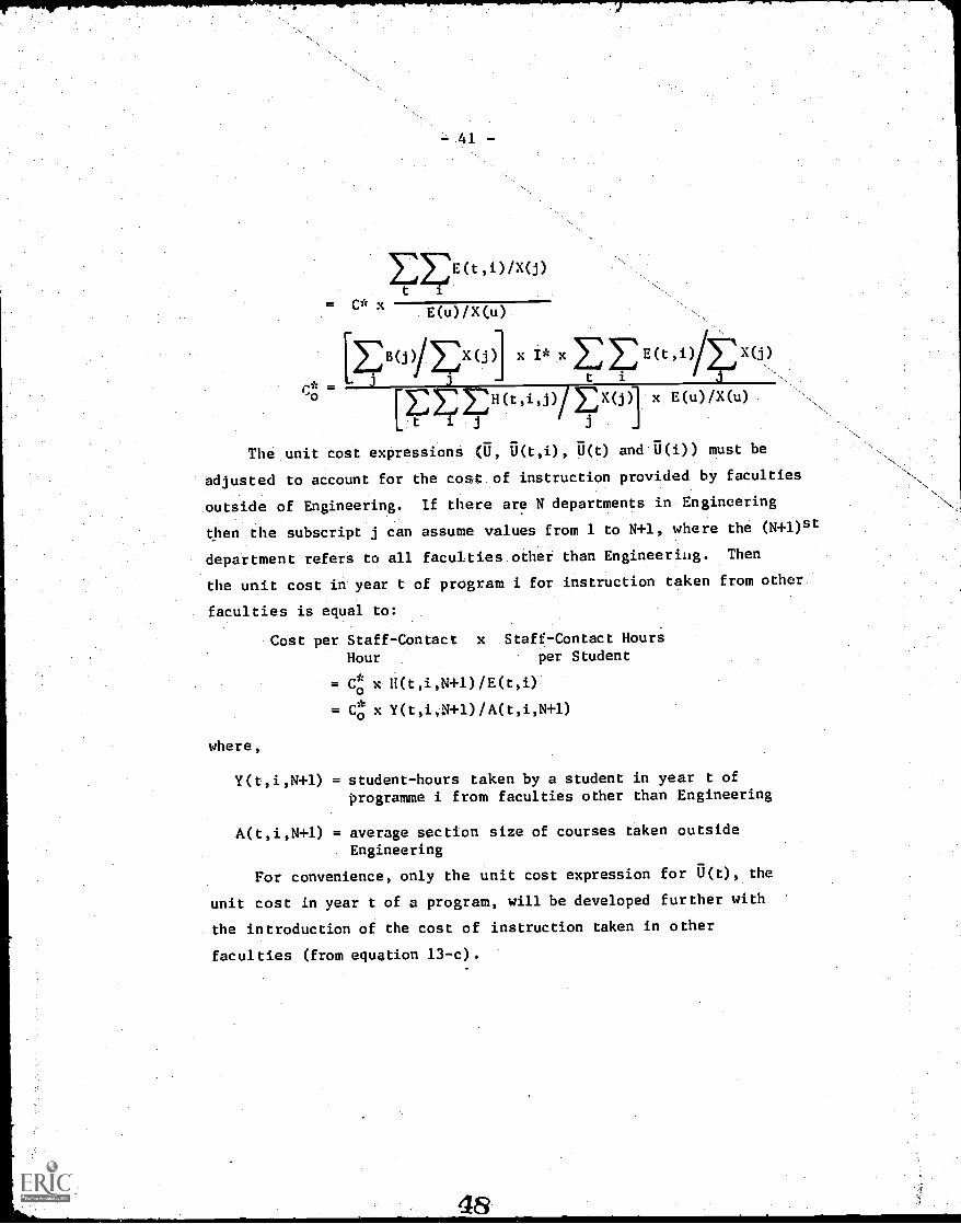
EEE(t,i)/X(j)t
= C* x E(u)/X(u)
BOVEK(j)] x I* x 2222 E(t,i) EX(j)
0* _ 3t i
o :E2H(t,i,j)if EX(j) x E(u)/X(u)
The unit cost expressions 0, U(t,i), U(t) and U(i)) must be
adjusted to account for the cot of instruction provided by faculties
outside of Engineering. If there are N departments in Engineering
then the subscript j can assume values from 1 to N+1, where the (N+1)st
department refers to all faculties other than Engineering. Then
the unit cost in year t of program i for instruction taken from other
faculties is equal to:
Cost per Staff-Contact x Staff-Contact Hours
Hour per Student
= Co x H(t,i,N+1)/E(t,i)
Co x Y(t,i,N+l)/A(t,i,N+l)
where,
Y(t,i,N+1) = student-hours taken by a student in year t ofprogramme i from faculties other than Engineering
A(t,i,N+1) = average section size of courses taken outside
Engineering
For convenience, only the unit cost expression for U(t), the
unit cost in year t of a program, will be developed further with
the introduction of the cost of instruction taken in other
faculties (from equation 13-c).
U(t) = unit
-42-
cost in year t
Cost of instruction Cost of instruction fromin Engineering other Faculties
x
(Equationsequations
1
A(t,i) E E H(t,i,j)/X(j)J =1
B(j)/X(j)
x I(j) x Y(t,i,j)
t
B(j)A X(j)] x I* x EEEct,i/Ex(i)J=1 t 717
EEEH(t,i,j/tX(j) x E(u) /X(u)t i j =1. j=1
Y(t,i,N+1)1
A(t,i,N+1)
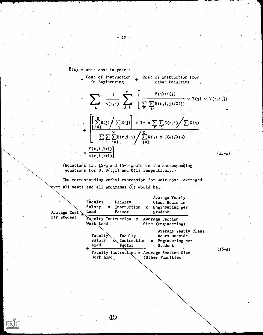
15, 15-a and 15-b would be the correspondingfor U, U(t,i) and U(i) respectively.)
The corresponding verbal expression for unit cost, averaged
aver all years and all programes (U) would be;
Average Costper Student
Faculty FacultySalary x InstructionLoad Factor
\\
Faculty InstructionWok,Load
FacultySalaryLoad
Faculty InstructWork Load
Average YearlyClass Hours in
x Engineering perStudent
x Average SectionSize (Engineering)
Average Yearly ClassHours Outside
x Engineering perStudent
FacultyInstructionFactor
49
on x Average Section Size(Other Faculties
(15-c)
(15-d)
- 43 -
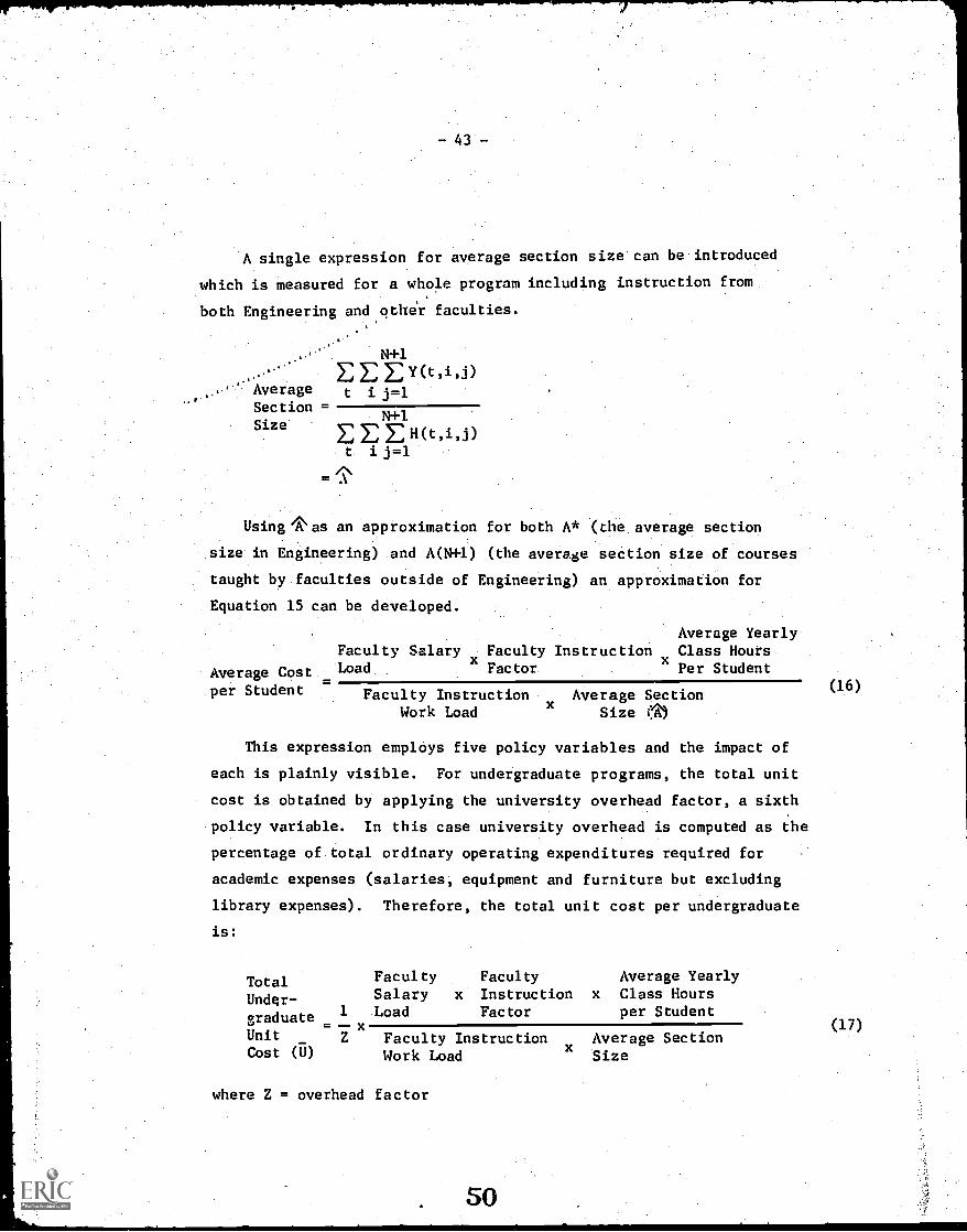
A single expression for average section size can be introduced
which is measured for a whole program including instruction from
both Engineering and other faculties.
N+1Y(t,i,j)
Average t i j=1
SectionN+1
Size E H(t,i,j)t i j=1
= A/\
Using rkas an approximation for both A* (the. average section
size. in Engineering) and A(N41) (the average section size of courses
taught by faculties outside of Engineering) an approximation for
Equation 15 can be developed.
Average YearlyFaculty Salary Faculty Instruction Class Hours
Average Cost _x Factor Per StudentLoad
x
per Student Faculty Instruction Average SectionWork Load
xSize (13
This expression employs five policy variables and the impact of
each is plainly visible. For undergraduate programs, the total unit
cost is obtained by applying the university overhead factor, a sixth
policy variable. In this case university overhead is computed as the
percentage of total ordinary operating expenditures required for
academic expenses (salaries, equipment and furniture but excluding
library expenses). Therefore, the total unit cost per undergraduate
is:
TotalUnder-
graduate
Faculty Faculty Average YearlySalary x Instruction x Class Hours
1 Load Factor per Student
Unitx
_ Z Faculty Instruction Average SectionCost (U) Work Load x Size
where Z = overhead factor
50
(16)
44 -
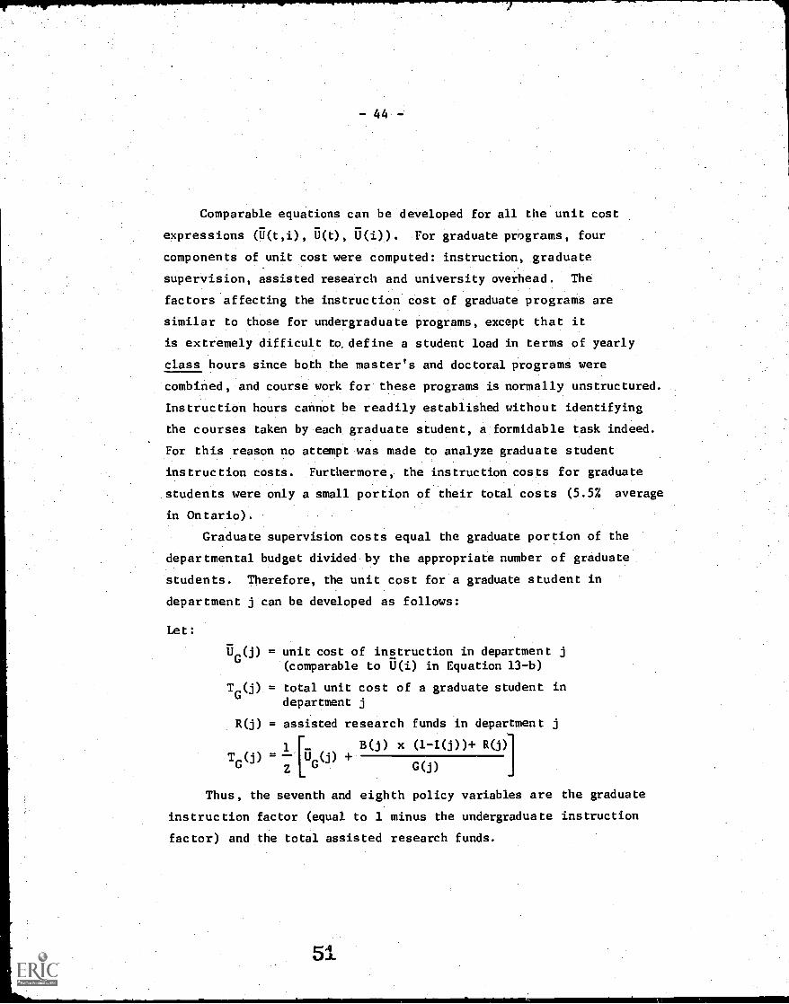
Comparable equations can be developed for all the unit cost
expressions 6.1(t,i), U(i)). For graduate programs, four
components of unit cost were computed: instruction, graduate
supervision, assisted research and university overhead. The
factors affecting the instruction cost of graduate programs are
similar to those for undergraduate programs, except that it
is extremely difficult to. define a student load in terms of yearly
class hours since both the master's and doctoral programs were
combined, and course work for these programs is normally unstructured.
Instruction hours cannot be readily established without identifying
the courses taken by each graduate student, a formidable task indeed.
For this reason no attempt was made to analyze graduate student
instruction costs. Furthermore, the instruction costs for graduate
students were only a small portion of their total costs (5.5% average
in Ontario).
Graduate supervision costs equal the graduate portion of the
departmental budget divided by the appropriate number of graduate
students. Therefore, the unit cost for a graduate student in
department j can be developed as follows:
Let:
UG
= unit cost of instruction in department j(comparable to U(i) in Equation 13-b)
T (j) = total unit cost of a graduate student indepartment j
R(j) = assisted research funds in department j
T (j) 'G0) +
1 -
G(j)
x (1-I(j))+ R(j)
Thus, the seventh and eighth policy variables are the graduate
instruction factor (equal to 1 minus the undergraduate instruction
factor) and the total assisted research funds.
-45-
6. SUMMARY AND CONCLUSIONS
The policy variables that were identified in the last section can
be used as a tool to control unit costs at any, or all, of the three
administrative levels: university, faculty and department.
1. Salary Load (Budget per FTE staff) - Since the majorportion of a departmental budget is salary, thisquantity reflects the mixture of senior and juniorstaff in the department, the general age-experienceprofile and the current salary levels. This factor
tend:, to be high for new institutions where attrac-tive salaries and positions must be offered toattract qualified staff. As the university grows,this factor will tend to decrease, but when stabilityis achieved, it may increase as staff are promotedthrough the ranks. Therefore this factor can becontrolled through salary increases, promotion andtenure policies and the use of part-time staff. For
example, the use of part-time teaching staff fromthe profession should influence. the factor in a down-
ward direction.
2. Instruction Factor (Percentage) - This factor reflectsthe relative emphasis placed on undergraduate education.A low instruction factor shifts the expenditure from theundergraduate to the graduate sector. The instruction
factor tends to decrease as the number of graduatestudents increases, and the result is that fewer hourscan be devoted to instruction for a fixed total staff
workload. This creates a need to reduce the number of
sections leading to larger section sizes, particularlyin the first and second year.
3. Student Load (Yearly hours of course instruction perstudent) - This factor represents the amount of timeeach student is required to spend in. course instruc-
tion. Because of accreditation requirements andtraditions, engineering programs tend to involvestudents in comparable instruction times and there-fore this quantity exhibits the least amount of
variation. Some of the variation may be accountedfor by differences in the number of weeks in the
academic year. Any adjustment of this variable mustresult from a value judgment related to the number ofhours a student should spend in class as opposed to
other activities.
4. Instruction WorPload (Staff-contact hours per FTE staff) -This is only an approximate measure of the average facultyworkload since no explicit recognition is given to admini-strative duties, community or counselling services. There
is only limited control of this variable because of tradi-tion and normal university practices. The use of junior
-46-
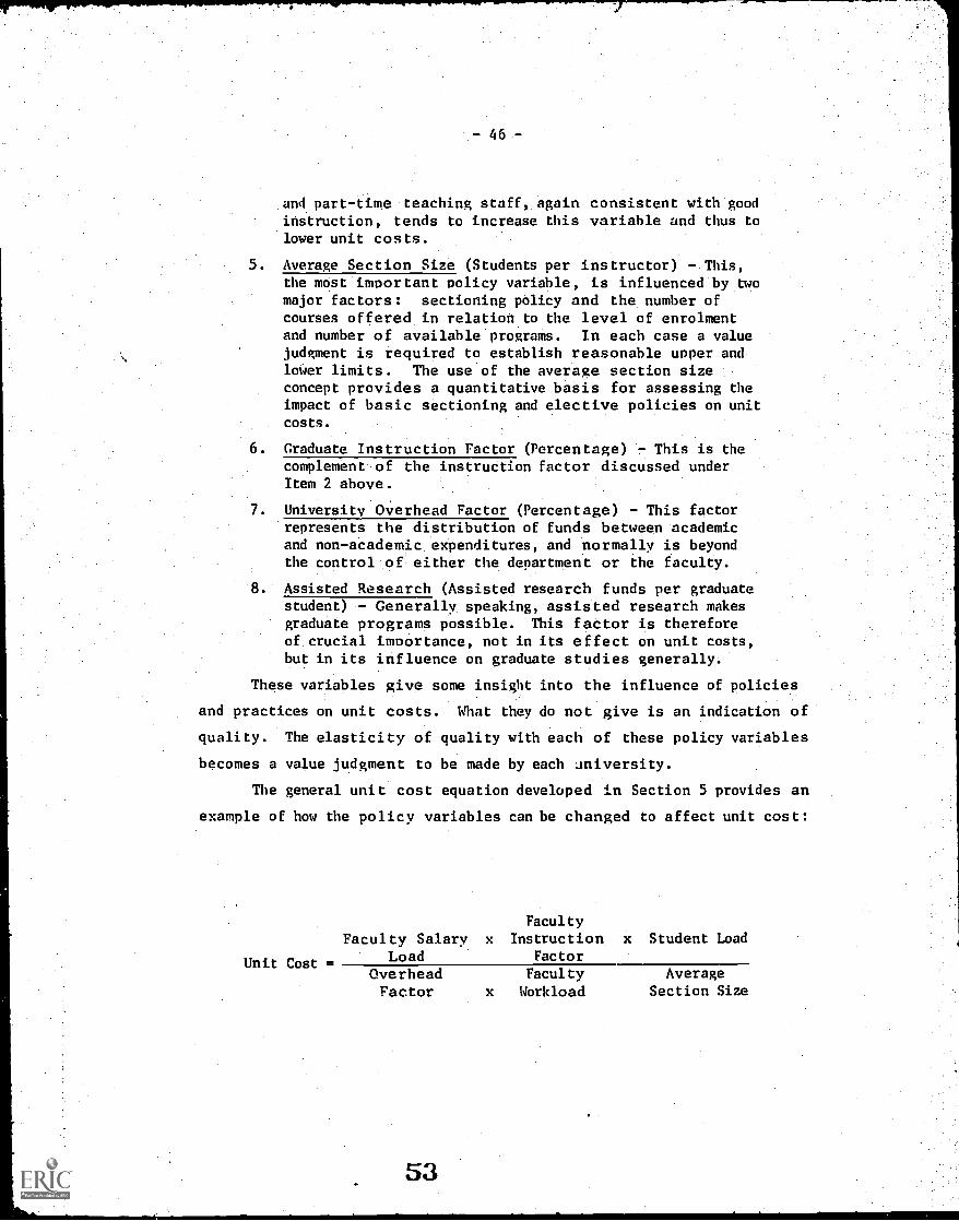
and part-time teaching staff, again consistent with goodinstruction, tends to increase this variable and thus tolower unit costs.
5. Average Section Size (Students per instructor) - This,the most important policy variable, is influenced by twomajor factors: sectioning policy and the number ofcourses offered in relation to the level of enrolmentand number of available programs. In each case a valuejudgment is required to establish reasonable upper andlower limits. The use of the average section sizeconcept provides a quantitative basis for assessing theimpact of basic sectioning and elective policies on unitcosts.
6. Graduate Instruction Factor (Percentage) - This is thecomplement of the instruction factor discussed underItem 2 above.
7. University Overhead Factor (Percentage) - This factorrepresents the distribution of funds between academicand non-academic expenditures, and normally is beyondthe control of either the department or the faculty.
. Assisted Research (Assisted research funds per graduatestudent) - Generally, speaking, assisted research makesgraduate programs possible. This factor is thereforeof crucial importance, not in its effect on unit costs,but in its influence on graduate studies generally.
These variables give some insight into the influence of policies
and practices on unit costs. What they do not give is an indication of
quality. The elasticity of quality with each of these policy variables
becomes a value judgment to be made by each university.
The general unit cost equation developed in Section 5 provides an
example of how the policy variables can be changed to affect unit cost:
Unit Cost =
Faculty SalaryLoad
OverheadFactor
Faculty
x Instruction x Student LoadFactorFaculty Average
x Workload Section Size
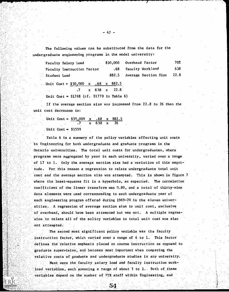
-47-
The following values can be substituted from the data for the
undergraduate engineering programs in the model university:
Faculty Salary Load
Faculty Instruction Factor
Student Load
$30,000 Overhead Factor 70%
.68 Faculty Workload 638
882.5 Average Section Size 22.8
Unit Cost = $30,000 x .68 x 882.5
.7 x 638 x 22.8
Unit Cost = $1768 (cf. $1779 in Table 6)
If the average section size was increased from 22.8 to 26 then the
unit cost decreases to:
Unit Cost = $30,000 x .68 x 882.5
.7 x 638 x 26
Unit Cost = $1550
Table 6 is a summary of the policy variables affecting unit costs
Engineering for both undergraduate and graduate programs in the
Ontario universities. The total unit costs for undergraduates, where
programs were aggregated by year in each university, varied over a range
of 17 to 1. Only the average section size had a variation of this magni-
tude. For this reason a regression to relate undergraduate total unit
cost and the average section size was attempted. This is shown in Figure 7
where the least-squares fit is a hyperbola, as expected. The correlation
coefficient of the linear transform was 0.89, and a total of thirty-nine
data elements were used corresponding to each undergraduate year of
each engineering program offered during 1969-70 in the eleven univer-
sities. A regression of average section size to unit cost, exclusive
of overhead, should have been attempted but was not A multiple regres-.
sion to relate all of the policy variables to total unit cost was also
not attempted.
The second most significant policy variable was the faculty
instruction factor, which varied over a range of 4 to 1. This factor
defines the relative emphasis placed on course instruction as opposed to
graduate supervision, and becomes most important when comparing the
relative costs of graduate and undergraduate studies in any university.
Next were the faculty salary load and faculty instruction work-
load variables, each spanning a range of about 3 to 1. Both of these
variables depend on the number of FTE staff within Engineering, and
54
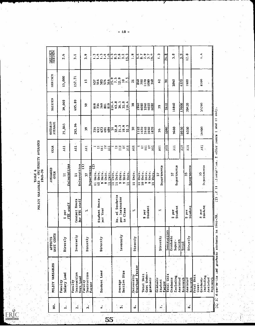
NO.
POLICY VARIABLES
AFFECTS
UNIT COSTS
Faculty
Salary Load
Directly
Faculty
Instruction
Work Load
Inversely
3.
Faculty
.Instruction
Factor
Directly
.
4.
Student Load
Directly
5.
Average
Section Size
Inversely
6.University
Overhead Factor
Directly
Total Unit
Cost Under-
graduate
Graduate
Student
Factor
Directly
Total Unit
Graduate.
Excluding.
Assisted
Research
Instruction
Graduate
Super -
vision
Total
Assisted
Research
Directly
Total Unit
Cost--
Graduate-
Including
Assisted
.Research
TABLE 6
POLICY VARIABLES - UNIVERSITY AVERAGES
1969-70
AVERAGED
OVER
YEAR
ONTARIO
AVERAGE
MAXIMUM
MINIMUM
MAXIMUM
MINIMUM
$ per
11
All
25,845
39,049
15;000
2.6
FTE staff
Universities
Contact Hours
11
All
293.96
495.89
157.71
3.1
Per FTE staff.
Universities
(1)
37
All
39
59
15
3.9
Departments
11 Univ.
(2)
1734
819
637
1.3
Student Hours
10 Univ.
11
652
736
514
1.4
per Year
9 Univ.
III
673
769
583
1.3
9 Univ.
IV
691
801
574
1.4
11 Univ.
All
689
819
514
1.6
11 Univ.
151
116.4
25.9
4.5
No. of Students
11 Univ.
II
32.8
63.8
7.5
8.5
per Instructor
9 Univ.
III
21.3
36.5
12.9
2.8
in Class
9 Univ.
IV
19.9
31.8
10
3.2
11 Univ.
All
32.3
116.4
7.5
15.5
%11 Univ.
All
30
38
21
1.8
11 Univ.
I1110
1960
860
5.4
per
$ p
10 Univ.
II
1670
6080
700
1170
8.7
2.9
Student
9 Univ.
9 Univ.
III IV
2140
2450
3360
4020
1080
3.7
11 Univ.
All
1820
6080
360
16.,'
37
Departments
All
70
79
62
1.3
All
1090
2410
90
26.8
$ per
37
All
9460
14860
3860
3.8
Student
Departments
All
10550
17000
4370
3.9
$er
Stupdent
35
Departments
All
6350
20420
1600
12.8
S per
Student
35
Dvpartmonts
All
16900
35290
8100
4.4
CI; 3: chpartm-nts ;.ad Araduato students in 196970.
:2) -f 11
_%1,:ersit:es. 2 offer years
Iand II only.
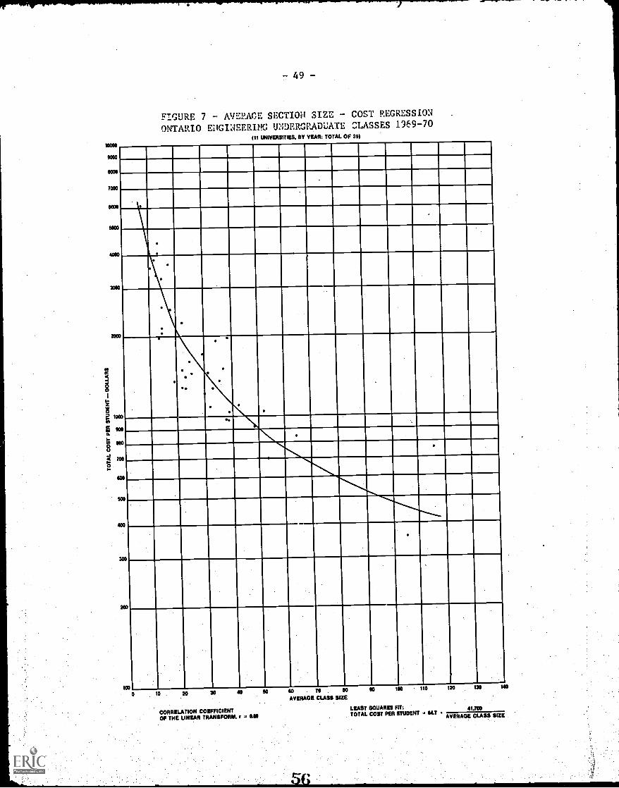
10000
9000
4000
7000
6000
5000
4000
3000
2000
UI
p.2 1000on
g 900
o I00
44 700
O.
600
500
400
MO
49
FIGURE 7 AVERAGE SECTION SIZE COST REGRESSION
ONTARIO ENGINEERING UNDERGRADUATE CLASSES 1969-70(11 UNIVERSITIES, BY YEAR: TOTAL OF 39)
0
200
1000 10 20 40 60 70 00
AVERAGE CLASS SIZE
CORRELATION COEFFICIENTOF THE UNEAR TRANSFORM, r 0.119
90 100 no 120 130 140
LEAST SQUARES FIT: 41.700TOTAL COST PER STUDENT = 64,7 AVERAGE CLASS SIZE
-50-
errors could have been introduced in the way they were reported by
each university and counted for the purposes of this study. Fortunately,
this counting does not affect unit cost calculations, since the number
of FTE staff cancel in the division of these two factors. The remain-
ing policy variables - university overhead factor and student load -
vary over a range of about 2 to 1, and so were the least influential.
It should be noted that student load and instruction workload
are not entirely independent. For example, if the academic year was
extended by an extra week, both policy variables would increase in
equal proportion. On the other hand, should extra classes be added to
the student load, then the instruction workload may or may not increase.
The extra staff load could be accommodated either by adding more staff
or by increasing the workload of the existing staff.
The dominant impact on graduate student costs, excluding assisted
research, was the graduate student factor. This resulted from the K
factor analysis which concluded that each graduate student used 150 staff
hours per year - an average for all of the engineering schools in Ontario.
Where there is a relatively large number of course-work master's students,
compared to thesis master's and doctoral students, unit costs would be
disproportionately high. The reverse may be true where graduate thesis
students predominate.
Assisted research accounts for about 40 percent of the total
unit costs for graduate students and includes income from many sources.
This additional cost would apply only to thesis students. It is an
external policy variable, principally under the control of the National
Research Council, that provides the major source of funds in response to
proposals for research grants from the universities.
In general, program unit costs increased with the year level,
principally because of the decrease in average class size in the later
years as illustrated in Table 7. This reduction in class size is caused
by decreasing enrolments due to attrition and the expansion of elective
courses in many programs, particularly in the third and fourth year.
- 51 -
TABLE 7
AVERAGE SECTION SIZE BY YEAR (UNDERGRADUATE)
UndergraduateYear
Average Section Size(Ontario)
Number ofStudents in Sample
I 54.5 2,621
II 34.3 2,450
III 21.3 1,709
IV 19.9 1,446
All 32.0 8,226
One important product of the cost study was the effect of engineer-
ing school size on unit costs. Figure 8 is a cost-size comparison, and
shows how the unit cost varied with the number of students in under-
graduate programs (eleven universities). It is difficult to draw firm
conclusions with such a small number of points, but a trend appears to
emerge; the curve exhibits .a minimum band below which classes are
small because they are student-limited. Within the band, classes reach
a critical size, where sectioning becomes necessary. Beyond the band,
sectioning policy is the main determinant, and as the school becomes
very large, there appears to be a tendency to section into smaller
classes. In the larger schools, more elective classes are offered in
the third and fourth year, and this tends to keep average section size
down even though total student numbers are relatively large.
From Table 5, it is possible to estimate very roughly the expendi-
ture required for an engineering degree. A crude attrition model is
assumed as follows: 75 percent second year survival from first year,
85 percent third year survival from second year, 90 percent fourth year
survival from third year and 95 percent degree survival from fourth
year. A conditional probability calculation was carried out using this
model for the class of 1970. In round numbers, the expenditure to
produce a graduate engineer in 1970 was about $8,000, provided the
structure developed in the cost study did not alter appreciably over
the previous three years.
- 52 -
FIGURE 8 - COST-SIZE COMPARISONONTARIO ENGINEERING SCHOOLS 1969-70
1M IMOD
ONTARIO AVERAGE- UNDERGRADUATE AND GRADUATE STUDENTS (EXCLUDING ASSISTED RESEARCH)
ONTARIO AVERAGE- UNDERGRADUATE STUDENTS4 .f
MINIMUM BAND
UNDERGRADUATE COSTS
NUMBER OF UNDERGRADUATE STUDENTS
-53-
If attrition and discount are neglected for graduate students,
the additional expenditure for a master's degree achieved in one year
after the bachelor's degree was $8,190 (a total of about $16,000).
For a doctorate achieved in four years after the bachelor's degree,
there was an additional expenditure of $33,000 (a total of $41,000)
excluding assisted research, or an additional exnenditure of $54,000
(a total of $62,000) including assisted research.
- 54 -
7. OVERVIEW
Does this methodology for undertaking a cost study have universal
applicability? In this study we have applied the method to a discipline
within the Ontario university system. We believe the method should be
valid for other disciplines provided there are sufficient data points
to establish a value for the K factor. However, it is difficult to
ascertain whether the method could be applied to a single institution
because it would be necessary to assume a common relationship between
the cost of a graduate student and the cost of a staffrcontact hour for
several disciplines in order to accumulate enough data points for the
regression.
The major problem arises from the attempt to distribute a depart-
mental budget between graduate supervision and formal instruction. This
is the golden fleece that many Argonauts have sought. Whether or not
we have been successful in coming closer to achieving that goal will be
judged by time and future study.
The introduction of the policy variables and the unit cost equations
should prove most useful to administrators.
In conclusion, we would wish to save future data combatants from
having to wade through massive calculations and manipulations. After
handling data sets for several weeks, it became evident that the calcula-
tions resolve to a few basic matrix multiplications. For the next
adventurer these have been outlined in Appendix C. We do not mean to
imply that the task of deriving unit costs has been reduced from its
herculean proportions; budget and enrolment data must still be assembled,
and a staff-contact hour matrix derived. But given these data sets, the
task of producing unit costs should be lightened through matrix multi-
plication.
APPENDIX A
(Basic Data - Model University)
-56-
TABLE A-1
BASIC DATA - MODEL UNIVERSITY
FTE ENROLMENT
Year 1 Year 2 Masters PhD Total
General 500 500
Civil Engineering 250 80 20 350
MechanicalEngineering - 150 - - 150
Total Engineering 5(Y) 400 80 20 1000
Total University N.A. N.A. N.A. N.A. 10000
N.A. - not applicable
Engineering FTE Staff - 50
University FTE Staff 625
Length of Session - 25 weeks
TABLE A-2
COURSE ENROLMENT DATA
Course
Given by the
staff
of
the Dept. of
Number of
sections
Given to
students in
Number of students
from each program
Total annual contact
hours per st(dent
Total annual staff
hours per section
Lec.
Lab.
Tut.
Lec.
Lab.
Tut.
Lec.
Lab.
Tut.
*Structures
Civil
5General-1
500
100
100
Materials
Civil
12
General-1
500
500
100
100
100
600
Forestry-1
'100
100
Water resources
Civil'
5Civil-2
250
250
200
200
200
Steel structures
. Civil
5Civil-2
250
250
100
150
100
300
Transportation
Civil
1Civil-Grad.
10
100
100
Systems .dynamics
Mechanical
10
General-1
500
500
100
150
100
400
Vibrations
Mechanical
10
General-1
500
500
100
150
150
200
Physics-1
250
Materials science
Mechanical
20
Mechanical-2
150
100
100
Civil-2
250
Fluid mechanics
Mechanical
5Mechanical-2
150
150
100
100
100
600
Physical metallurgy
Met. & Mat. Sci.
5Civil-2
250
250
100
150
200
500
Materials science
,Met. & Nat. Sci.
3Mechanical-2
150
150
50
100
150
250
Physics of metals
Net. & Mat. Sci.
2Mechanical-2
150
100
100
Statistics
Mathematics
5General-1
500
500
100
100
100
300
refers to 1st year in the General Engineering program - based on the following format "PROGRAM - YEAR INPROGRAM"
- 58 -
TABLE A-3
noDEL UNIVERSITY - BUDGET DATA
UNIVERSITY
Total academic expenditures as a percentage oftotal ordinary operating expenditures 70%
FACULTY OF ENGINEERING
,
Department
AcademicSalaries
$
OtherExpenses
$
.
Total$
AssistedResearch
$
Civil 400,000 200,000 600,000 300,000
Mechanical 300,000 100,000 400,000
Metallurgy andMaterials Science 150,000 50,000 200,000
FacultyAdministration N.A. N.A. 300,000
TOTAL 850,000 350,000 1,500,000 300,000
N.A. - not applicable
APPENDIX B
(List of Symbols)
- 60 -
The following are the common symbols used in the report:
C(j) instruction cost per staff-contact hour in department j
H(t,i,j) staff-contact hours devoted to year level t of program i
by department j
E(t,i) enrolment in year level t of program i
e(u) enrolment for whole university
D(t,i,j) instruction cost per student in year level t of orogram i
for department j
G(j) number of graduate students supervised in department j
0.(j)teaching equivalents in department j
1(j) instruction factor for department j
S(j) graduate student factor for department j
B(j) budget for department j
X(j) number of FTE faculty in department j
X(u) number of rTE faculty in the university
T(t,i) total cost of year t in program i
17(t,i) unit cost of year t in program i
U(i) unit cost in program i
U(t) unit cost in year t
U unit cost (averaged over all programs and years)
C* faculty cost per staff-contact hour - Engineering
faculty cost per staff-contact hour - other faculties
faculty instruction factor
A*
yearly student hours by year t of prpgram i from department
faculty average section size
average sectio:.vsize for a whole program
-61-
A(t) average section size of courses taken by students in year t
A(i) average section size of courses taken by students in program i
A(N+1) average section size of courses taught by faculty outside ofengineering
Z overhead factor
UG(j) unit cost of graduate instruction in department j
TG
total unit cost of a graduate student in department j
R(j) assisted research funds in department j
68
APPENDIX C
(Unit Cost Analysis - Matrix Format)
69
-63-
UNIT COST ANALYSIS - MATRIX FORAT(1)
Given: k - scalar - the K factor
H = (hi 1j - staff-contact hour matrix i = 1,n
j = 19m
hij = staff-contact hours taught by department j to program i
S = s 0 - n x n diagonal matrix
LO sn
si = undergraduate students enrolled in program i
[
B = bi.
0
0
bm
- m x m diagonal matrix
bi = budget for department i
G = gi 0. - m x m diagonal matrix
[0 gm
gi
= graduate enrolment in department i
(1) The authors are deeply indebted to Professor Bernard Etkin, Institute
for Aerospace Studies, University of Toronto, who, when we were
entangled in mathematical manipulations, showed us this shortcut, then
reviewed this presentation and corrected our mistakes.
70
Define:
-64-
= ml 0 -mxmdiagonal matrix
0 mm
m. = staff-contact hours taught by department i
E
I
1-mxmdiagonal matrix
0em
ei = teaching equivalents for department i
H* -mxmrectangular matrix
hid = staff-contact hours per student in program i taught by
department 1
u
ui
c
C
= (u.)
= unit cost of a student
= (c.)1
= c1
0
[0cm
- n x 1 column matrix
in program i
m x 1 column matrix
-mxmmatrix
c. = cost per teaching equivalent in department i
Therefore:
-65-
e = m + kgE = M + kG
H = SR*
H* = S-111
--I
where, S1 = 0
0 s-1
n
u = H*c
II* =S-.1li
u = S-1Hc
B = CE
C = BE-1
c = CA
where, A
1
= RE-1A
u = S-1
HBE
E = M + kG
mx 1 column matrix
u = S 1HB(M + kG) -1,1
Note: the ith
element of the diagonal matrix ('I + kG)-1
is
+ kgi)-1
72

![Sir William John Thompson Slides - rcpi-live-cdn.s3 ... · Sir William John Thompson Slides 2 WJTS Sir William John Thompson Slides Collection [1910s-1920s] Extent: 4 boxes Creator:](https://img.pdfslide.us/doc/110x75/5c0e07d709d3f258548c65ae/sir-william-john-thompson-slides-rcpi-live-cdns3-sir-william-john-thompson.jpg)