DOCUMENT RESUME

ED 259 002 TM 850 371

AUTHOR Nandakumar, RatnaTITLE An Application of Heckman's Correction for

Specification Error.PUB DATE Apr 84NOTE 35p.; Paper presented at the Annual Meeting of the

American Educatic al Research Association (68th, NewOrleans, LA, April 23-27, 1984).

PUB TYPE Speeches/Conference Papers (150) -- Reports -Research /Technical (143)

EDRS PRICE MF01 Plus Postage. PC Not Available from EDRS.DESCRIPTORS *Admission Criteria; College Entrance Examinations;

*Error of Measurement; Grade Prediction; GraduateStudy; Higher Education; Law Students; PredictiveMeasurement; *Predictive Validity; *Regression(Statistics); Sampling; *Selective Admission;*Statistical Bias

IDENTIFIERS *Heckman (J J); Law School Admission Test;Specification Bias

ABSTRACTBeckman's correction for regression in selected

samples for predictive validity studies was applied to a large datafile on 7,984 law school applicants. Data included ethnic group, sex,socioeconomic status, undergraduate degree, school, scores on the LawSchool Admission Test (LSAT), writing ability, undergraduate gradepoint averas.e, and age. The final selection criteria were not known.Data on the 1,845 applicants who were accepted included year ofentrance, sex, date of birth, undergraduate grade point average,grade point average for first year of law school, undergraduatecollege, LSAT score, writing ability, ethnic group, and age. Thegrade point average for the first year of law school was estimatedand compared, with and without using Heckman's correction factor.Three different methods were used to choose the variables for studentselection and grade prediction: (1) the same set of variables wereused for both selection and prediction; (2) a subset of variablesused for selection were used for prediction; and (3) two completelydifferent sets were used. It was found that the relation between thevariables used for selection and prediction could affect the accuracyof prediction. (Author/GDC)

************************************************************************ Reproductions supplied by EDRS are the best that can be made ** from the original document. *

***********************************************************************

Aa Application of Heckman's Correction for

Specification Error

Ratna Nandakumar

University150, CRC

Champaign,

of Illinois

Il 61820"PERMISSION TO REPRODUCE THISMATERIAL IN MICROFICHE ONLYHAS BEEN GRANTED BY

10ArciammaL,

TO THE EDUCATIONAL RESOURCESINFORMATION CENTER (ERIC)."

U.& DEPARTMENT Of EDUCATORNATIONAL INSTITUTE Of EDUCATION

EDUCATIONAL RESOURCES INFORMATIONCENTER (ERIC)

iiriiis document has been reproduced asreceived from the person or otgenicatl041originating it

11 Minor changes have been mods to impi0Vreproduction quality.

Points of wow or opinions staled in thismint do not necessarily moment oll..11NIEpositron or policy.

Paper presented at the annual meeting of the American EducationalResearch Association, New Orleans, April 1984

ABSTRACT

In this papaer an attempt is made to apply

Heckman's procedure for correction of specification

error in selected samples. A large law school data

set has been used in the study. The first year

average in law school is estimated and compared with

and without using Heckman's correction factor. Three

different ways are considered to select the variables

for selection and prediction: 1. The same set of

variables are used both for selection and prediction.

2. A subset of variables used for selection is used

for prediction. 3. Completely different sets of

variables are used for selection and prediction. It

was found that the relation between the variables used

for selection and prediction can affect the accuracy

of prediction.

4

1

Introduction

Predictive validity studies take place in situations where

individuals are selected on so.ne basis to meet a specified

criterion. If a test score is used as a basis of selection,

predictive validity is obtained by comparing test scores with

the criterion variable considered to provide a measure of the

characteristic in question. For example, in colleges and

universities students are selected on the basis of test scores

which predict their academic success or a firm hires people on

the basis of several factors that predict the job success.

Predictive validity studies are used to see if tests used for

selection predict the performance or a specified criterion. In

the example of college students one would want to know if

students selected on the basis of test scores perform better

than u,screened group of students i.e., to see if test used for

selection predicts the. performance. Decision makers use

predictive validity results for placement of people to

different treatments according to the test scores.

In such studies we often come across situations where the

selection of units into the sample is not random. In such

situations it is important to model the selection process (the

process by which the observed units are selected into the

sample). This is typical when the students are admitted into a

college. The Restrictive samples may also occur due to

2

attrition when the individuals voluntarily participate in the

program (self selection) and in longitudinal studies. Failure

to recognize the sample selection s.nd analysing the selected

samples as though it were random can have serious consequences

such as biased and inconsistent estimates of the parameters.

As said in Linn(1982), "Fortunately randomization is not the

only approach to obtaining unbiased estimates of mgression."

What is important is to avoid bias by gaining full knowledge

about the selection process and model it. Selectivity problems

have been discussed in various contexts by many authors, e.g.

Gonan (1974), Lews (1974), Heckman (1974, 1977), Goldberger

(1981) and Linn (1982).

Linn(1982) showed how tie selection process can produce

overprediction results for minority groups in two different

cases of populations.

the population

Case(1) There is no overprediction in

prior to selection;i.e., the regression

equations of majority and minority groups are equal. Case(2)

The majority group regression equation underpredicts the

average minority group performance in the population prior to

selection. For each of these two cases, three possible cases

of minority group selection is considered: 'a) random selection

or no selection. (b) selection on the basis of third variable

U defined as for the majority group selection. (c) selection

on the basis c U',which places less weight on X for

minority-group than for majority-group members.

l

1k

3

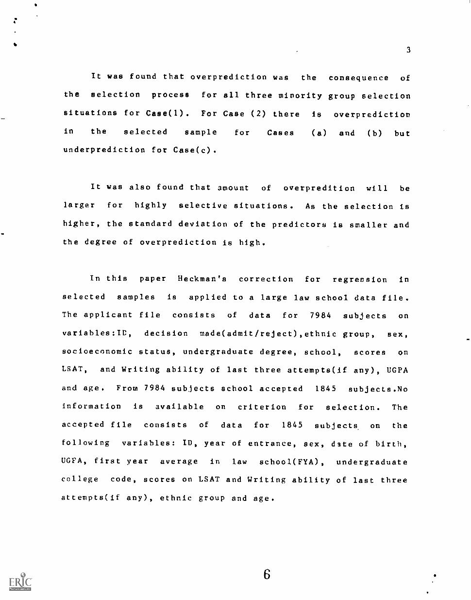
It was found that overprediction was the consequence of

the selection process for all three minority group selection

situations for Case(1). For Case (2) there is overprediction

in the selected sample for Cases (a) and (b) but

underprediction for Case(c).

It was also found that amount of overpredition will be

larger for highly selective situations. As the selection is

higher, the standard deviation of the predictors is smaller and

the degree of overprediction is high.

In this paper Heckman's correction for regression in

selected samples is applied to a large law school data file.

The applicant file consists of data for 7984 subjects on

variables:ID, decision made(admit/reject),ethnic group, sex,

socioeconomic status, undergraduate degree, school, scores on

LSAT, and Writing ability of last three attempts(if any), UGPA

and age. From 7984 subjects school accepted 1845 subjects.No

information is available on criterion for selection. The

accepted file consists of data for 1845 subjects, on the

following variables: ID, year of entrance, sex, date of birth,

UGFA, first year average in law school(FYA), undergraduate

college code, scores on LSAT and Writing ability of last three

attempts(if any), ethnic group and age.

4

4

The applicant file was used for Probit analysis to obtain

the parameters of 'equation (8) (explained below) and the

results are used to obtain Heckman's correction factor. The

accepted file was used for obtaining the least-squares

estimates of regression equations : (1) regression equation

with Heckman's correction factor. (2) regression equation

without Heckman's correction factor.

Method and application

Consider the simple regression of Y on X in the unselected

population,

(1) Y pe + p, x + 6

where c is un-nrrelated with X.

can

If one has random samples of observations on Y and X, one

obtain unbiased estimates of po and pi by ordinary least

squares (OLS). If the sampling is non random, the units are

selected on the basis of a possibly unobservable variable U.

The units are selected into the sample if U exceeds a threshold

value (say U > 0). In this case the residual is no longer

independent of X, and so the estimates will be biased as a

function of the sampling lrocess. As stated by Berk, Ray &

Cooley (1982), there are problems of external validity and

internal validity. First, the regression line for the original

population does not correspond to the regression line for the

5

selected population. The reg: 'on parameters differ

depending upon the data availdbl . This is a problem of

external validity. Second, the error term is correlated with

the regressor and this is a problem of internal validity. The

estimates of regression coefficients are biased and the linear

regression model is the wrong model even in the selected

population. This is conceived by Heckman as specification

error in the original model which has no parameter representing

the selection process. Conventional formulas for correcting

the restriction of range may not be appropriate due to the

limitation of underlying assumptions, i.e. linearity and

homoscedasticity. Furthermore,application of traditional range

restriction formulas requires that all variables,which

contribute to the selection process be included in the

analysis,but this is rarely possible since the percise basis of

selection is often unknown.

When U = X, i.e., when the selection is based explictly on

the independent variable, there is zero probability of

selecting population units to the left of this value. In this

case if the units to the right of U are selected at random,

then there is no specification error and OLS gives unbiased

estimators of po and pi However correlation estimates

between X and Y are affected because of reduced variance of X

in the selected population.

6

When U * Y, i.e., when the selection is based explicitly

on dependent variable, there is no probability of selecting

population units below (above) this value into the selected

population. In this case the error term will be correlated

with X in the sample. The mean of error values will be higher

for units with smaller X values. If U * 0, this corrsponds to

the Tobin(1958) model (correlation of limited dependent

variables). In this case OLS gives biased estimates of the

slope pj , which is biased downwords and is inconsistent for

large samples. The regression line in the selected population

will have a smaller slope and higher intercept. Under the

assumpt4.on of multivariate normality the relations due to

Goldberger ',1981),between the regression parameters in the

original and selected populations can be written as :

(2) f344=

(3) CC* (42)."1;

2.

(4) 14 c Where

(5) c (mod

(6)= VI(Y)10-2

where asterisks indicate the parameters in the selected

population.

7

Equations (2) and (4) show that the slope and the multiple

correlation coefficients in the selected population are

proportional to the slope and correlation coefficients in the

original population, the constant of proportionality being the

constant c The impact of selection is therefore represented

by constant c , which in turn depends on & From

Equation (6), G is the ratio of variance of the dependent

variable Y in the selected population to the variance in the

original population.

From Equations (5) & (6), assuming 0<r< 1, it can be seen

that, when 0 > 1.0, the constant c > 1.0 and the regression

a-2*coefficient /3* in the selected population is inflated. When

e <1.0, the constant c< 1.0 and the regression coefficent in

the selected population is deflated. When 0 = 1.0, the

regreosion coefficients are equal in both the populations.

Therefore the crucial point is the relation between the

variance of Y in the selected population and the original

population.

When V = 1, c = 1 and there is no effect due to

selection. For r . 0, c . 0 . But in reality /9 will not

take these extreme values. The intercept in the selected

population is also distorted.

8

The sample drawn from the selected population, therefore

produces inconsistent estimates of the regression parameters in

the original population, with a degree of inconsistency

depending on the value of the constant c . For example, when

c = 0.5 the estimated regression coefficinets will be

approxiristely half of the original values, if the usual linear

regression model is applied and hence the external and internal

validities are in doubt.

When U is a third variable used as a basis or selection

OLS in the regression of Y on X will be different for 4ifferent

suhpopulations and there will be a decrease in the slope and a

concommitLant increase in the intercept. For all cases Dunbar

(1982) has illustrated the results by simulation methods for

normally distributed variables.

In the case of U used as a (unobservable) third .variable

as the basis of selection, Heckman treats the regression as a

two stage equation model. One equation describes the

relationship between Y and X and the other describes the

selection process. Equation (1) can be replaced by two

equations:

(7) Y = po + x +E

(8) U GE, + x +

We assume that in the total population the joint distribution

of E and S is normal and independent of X with means zero and

11

9

the covariance matrix of C and is given by

aiSlEAO 3.1S 6ri:rj

ws tre TES = covariance between andand 5 ra.. variance of 6.

and GTS = variance of S . Consider she regression of 6 on ,

(9) Lo5

is uncorrelated with E and VJ (ISE. 107S

Without loss of generality it is assumed th*t GE =1 so that

The regression of Y on X for the selected population units with

U > 0 is

E (\/14 u >0) pc -f + E. CE. u a)(10)

But from using equations (8) and (9) in (10) we obtain

E (v1;< iu >0) 13i (C) I g - - )

Let

(12) A(X) = Go+GI X ,

and fO) is defined by

Equation (11) can be written as

(13) E (v/x u o) = x )

T. is clear that OLS regression of Y on X will not give a

consistent estimate of pi unless L = 0 i.e 0TE 7C)

10

Let P(z) denote 6he probability distribution of c and p(z)

denote the density function of We assume p(z) to be

symmetric about zero, so that p(z) = p(z). Then,

b ( )1) = t) (dA ) cuA

1)(A)

when o has the standard normal distribution,let160(2) and it(z)

denote the density and distribution function of S. (14) can be

written as:

) (I) "'A

In Equation (13), if the covariance between the error

terms Aa the Equations (7) & (8) is zero, the regression weight

associated with f(i) ), () is 0 and the effect of incidental

selection disappears. The function f(A ), which is a

monotonically decreasing function of , represents the

probability that an observation is selected into the sample.

If f( A) is large, the likelihood of inclusion into the sample

is large and vice versa. Also, f(A) is the expectation of the

error term in the selection equation after selection. After

selection,f(A ) in the selection equation is nonzero and if CA)

is not equal to zero, contributes for incidental selection in

Equation (13) and is correlated with the regressor.

11

In the first step of Heckman's procedure Gio is estimated on

the full sample by maximum likelihood probit analysis with the

dependent variable Y coded '1' if an individual is selected and

eS4cvv..4dIA'0' if an individual is not selected. The 141444-crtmmi values

from Equation (8) are then used to constuct f( )1). In the

second step OLS is applied to Equation (13), with the estimated

f ( A ) as an additional predictor. The resulting regression

coefficients and the intercept from Equation (13) are

consistent and unbiased. If the regressors in both the

Equation (7) and (8) are very similar, it is common to find

high multicollinearity between f( A ) and other regressors in

Equation (13) and this makes it difficult to determine the

importance of selection effects.

The conditional mean and variance of Y are given by:

(1,5) E(VIY, U>o) -= Po 1- 13i X t co 401)

(I 6) VaY ( I X (.)) *ld (E. (U >o)

oT.c. CU2- -f(A) L' + .{- (A)j

Least-squares solution for parameters, of Equation (13)

using the data from only the selected sample gives unbiased and

consistent estimators of the parameters provided the probit

model is correctly specified. The standard errors for

estimated values in Equation (13) are larger than those that

would be obtained the model were applied to the entire

14

12

sample. Heckman notes that the conventional forlulas for

standard error applies only when r(6,6) . Otherwise the

conventional standard errors are underestimates of true

standard errors. From Equation (14) it can be seen that f(A)

is a nonlinear function of X and hence the true regression of Y

on X is nonlinear. Also from Equation (16), since CO is not

equal to zero and f(A) is not a constant, the conditional

variance of Y is heterogenous. As stated above inclusion of

f( A) as an additional predictor in the true regression of Y on

X introduces considerable amount of collinearity. This added

collinearity also contributes to the instability of the OLS

estimators.

Generalizations to the multivariate case can be made in a

straightforward manner to p arbitrary predictors;

Let B' and G' be the vectors of regression coefficients. The

model can be written as:

where

Y= B'X +E and

U = C'X +D,

observed if U > 0=

not observed otherwise

Main analysis and results

15

13

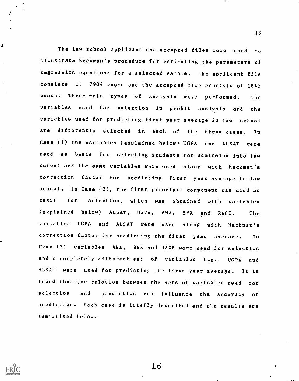
The law school applicant and accepted files were used to

illustratd Heckman's procedure for estimating the parameters of

regression equations for a selected sample. The applicant file

consists of 7984 cases and the accepted file consists of 1845

cases. Three main types of analysis were performed. The

variables used for selection in probit analysis and the

variables used for predicting first year average in law school

are differently selected in each of the three cases. In

Case (1) the variables (explained below) UGPA and ALSAT were

used as basis for selecting students for admission into law

school and the same variables were used along with Heckman's

correction factor for predicting first year average in law

school. In Case (2), the first principal component was used as

basis for selection, which was obtained with variables

(explained below) ALSAT, UGPA, AWA, SEX and RACE. The

variables UGPA and ALSAT were used along with Heckman's

correction factor for predicting the first year average. In

Case (3) variables AWA, SEX and RACE were used for selection

and a completely different set of variables i.e., UGPA and

ALSA" were used for predicting the first year average. It is

found that.the relation between the sets of variables used for

selection and prediction can influence the accuracy of

prediction. Each case is briefly described and the results are

summarised below.

16

14

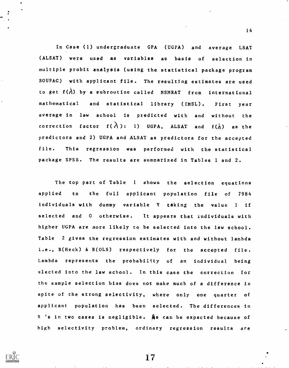
In Case (1) undergraduate CPA (UGPA) and average LSAT

(ALSAT) were used as variables as basis of selection in

multiple probit analysis (using the statistical package program

SOUPAC) with applicant file. The resulting estimates are used

to get f(A) by a subroutine called MSMRAT from international

mathematical and statistical library (IMSL). First year

average in law school is predicted with and without the

correction factor f(A): 1) UGPA, ALSAT and f(A) as the

predictors and 2) UGPA and ALSAT as predictors for the accepted

file. This regression was performed with the statistical

package SPSS. The results are summarized in Tables 1 and 2.

The top part of Table 1 shows the selection equations

applied to the full applicant population file of 7984

individuals with dummy variable Y taking the value 1 if

selected and 0 otherwise. It appears that individuals with

higher UGPA are more likely to be selected into the law school.

Table 2 gives the regression estimates with and without lambda

i.e., B(Heck) & B(OLS) respectively for the accepted file.

Lambda represents the probability of an individual being

slected into the law school. In this case the correction for

the sample selection bias does not make much of a difference in

spite of the strong selectivity, where only one quarter of

applicant population has been selected. The differences in

R 's in two cases is negligible. As can be expected because of

high selectivity problem, ordinary regression results are

17

15

biased. The corrected regression weights are higher than the

uncorrected ones. For predicting first yea: average in lawV6PA

school, variable 4114-7 appears to be a better predictor than

others. Even though the Lambda value is not statistically

significant, the direction of the impact seems reasonable.

Individuals who have high probability of being selected are

likely to have high first year averages. In this example, the

regressors used for selection and prediction equations are

exactly the same. This adds to the problem of

multicollinearity that follows even if the regressors are

different in two equations and hence contributes to the

reduction of selection effect. On the other hand, this also

implies that the correlations between the error terms in the

two equation model,i.e., 6) .=.3394 is too small for significant

selection effect, but indicates some selection effect. Berk,

Ray & Cooley (1982) note that the cross correlation between the

error terms often turn out to be small under properly specified

models. Consequently the selection artifacts will also be

small.

18

16

Summary of results for Case (1)

TABLE 1

1. Selection equation (1=applicanr selected)

Variable Max lik est Std.wt

UGPAALSATIntercept

1.12820.0052-7.9450

1.61E-020.02E-07

N = 7984No. selected = 1845

skafteterecustil

TABLE 2

Results in the selected sample

4

Corrected Uncorrected4

Variable B(Heck) p B(OLS) p

UGPA 1.1342 .354 0.8214 0

ALSAT 0.0130 .019 0.1161 0

LAMBDA 0.3394 .797

Constt

-5.0654 .595 -2.6217 .43

(1) Regression of FYA or. UGPA,ALSAT,LAMBDA :R = 0.5121 R = 0.2622Yh. -5.0656 + (1.1342) UGPA + (0.0130) ALSAT +

(0.3395) LAMBDA

(2) Regression of FYA with UGPA ALSAT :

R - 0.5121 RI = 0.2622Y. -2.6217 + (0.8215) UGPA + (0.0116) ALSATr ( Y

h,Ya) = 0.9999

19

11

In Case (2) the first principal component was computed

with the variables which included the average writing ability

(AWAB), ALSAT, UGPA, sex, and RACE from the original accepted

file. A pseudo accepted file was created from the original

accepted file with the top 500 cases on the first principal

component. The original accepted file with the additional

decision vector (1 if selected, 0 otherwise) was used for

probit analysis and the results were used to get f(A) as in the

Case (1) using SOUPAC and IMSL packages. The regression is

performed on the pseudo accepted file to predict first year

average with predictors 1) UGPA, ALSAT, f(),) and 2) UGPA,

ALSAT.The results are summarized in Tables 3 and 4.

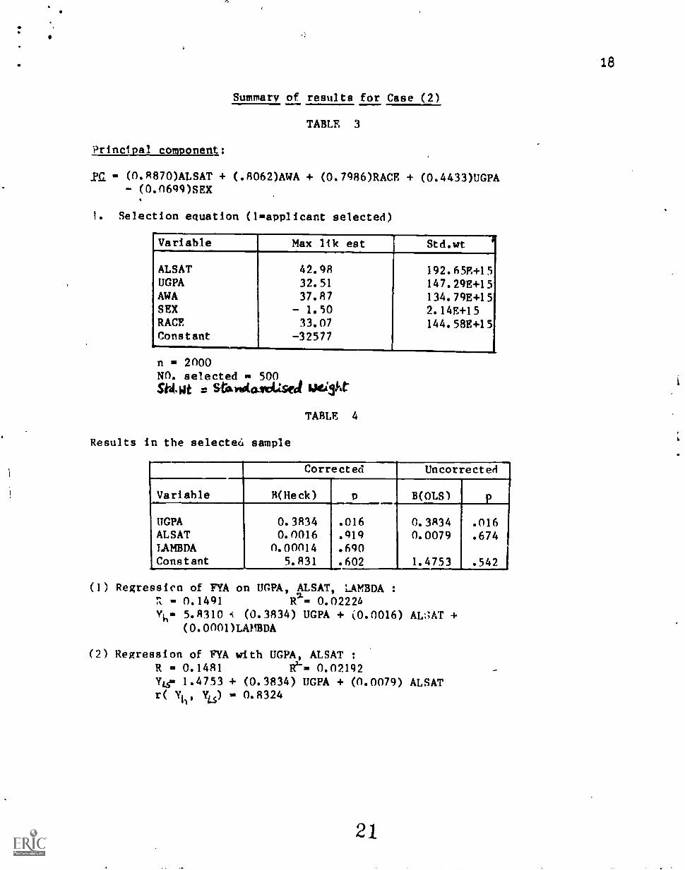
From Table 3,it can be seen that individualb with higher

scores of ALSAT are more likely to be selected, although

UGPA,AWA,and RACE also contribute very highly for selection.

Table 4 gives the regression estimate with and without the

correction factor which were computed for individuals in the

pseudo selected file. For this case, UGPA contributes

significantly for predicting the first year average. As can be

expected as a result of double selection, the variability of

predictors is very low and so R values are very small.The

correction factor for sample bias is nearly zero.It does not

make any difference for prediction whether LAMBDA is used or

not.

20

18

Summary of results for Case (2)

TABLE 3

Principal component:

.P.C. (0.R870)ALSAT + (.R062)AWA + (0.7986)RACE + (0.4433)UGPA

(0.0699)SEX

1. Selection equation (1- applicant selected)

Variable Max lik eat Std.wt

ALSAT 42.98 192.65E+15UGPA 32.51 147.29E+15AWA 37.87 134.79E+15SEX - 1.50 2.14E+15RACE 33.07 144.58E+15Constant -32577

n 2000NO. selected u 500Sititt = Stimput04141sed

TABLE 4

Results in the selecteo sample

Corrected Uncorrected

Variable H(Heck) p B(OLS) .

UGPA 0.3834 .016 0.3834 .016ALSAT 0.0016 .919 0.0079 .674LAMBDA 0.00014 .690Constant 5.831 .602 1.4753 .542

(1) Regression of FYA on UGPA, ALSAT, LAMBDA :

0.1491 R 0.02224Yku 5.8310 i (0.3834) UGPA + (0.0016) AL1;AT +

(0.0001)LAMBDA

(2) Regression of FYA with UGPA, ALSAT :R u 0.1481 /e.. 0.02192

Y1= 1.4753 + (0.3834) UGPA + (0.0079) ALSATr( 0.8324

21

19

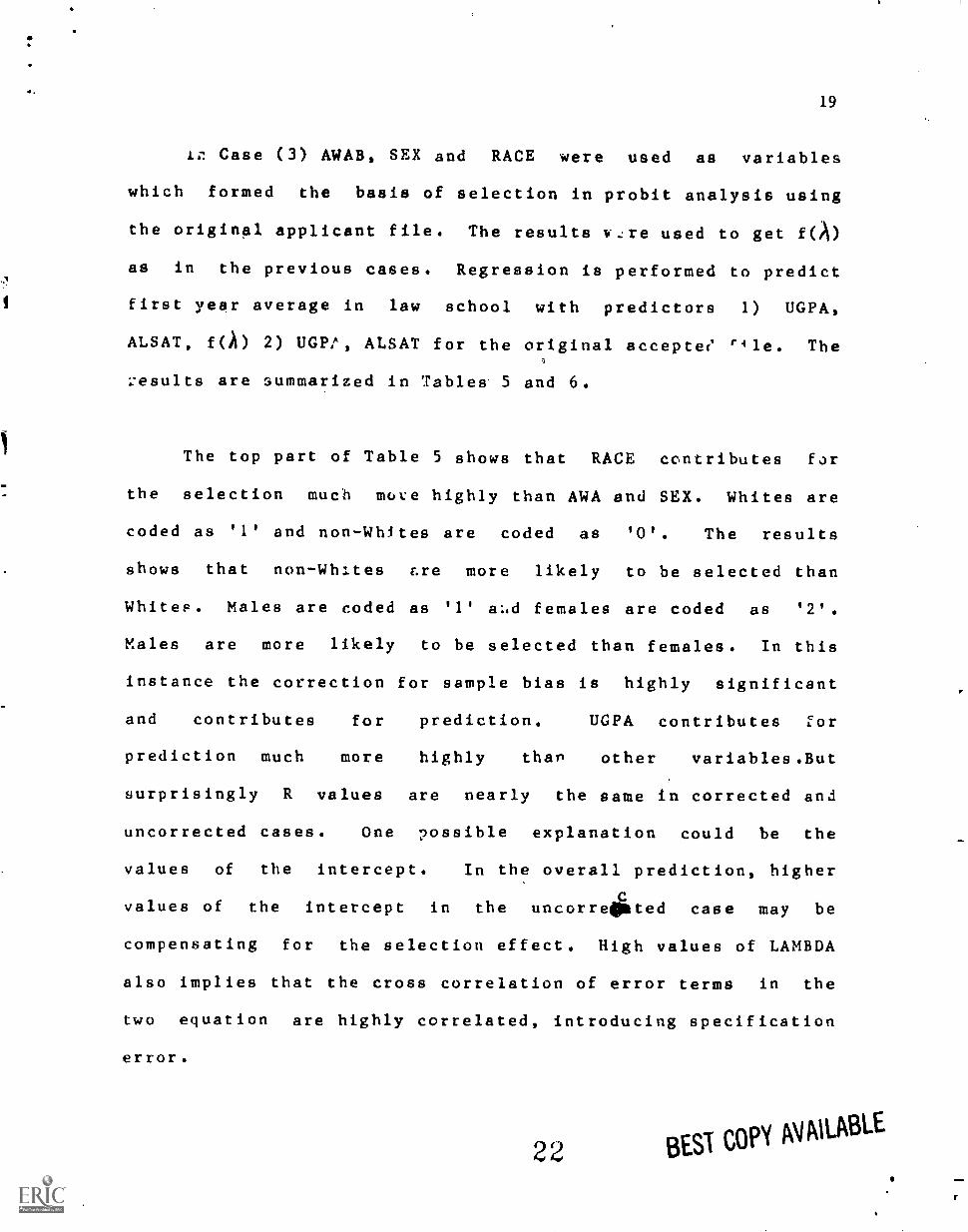
1:: Case (3) AWAB, SEX and RACE were used as variables

which formed the basis of selection in probit analysis using

the original applicant file. The results v..:re used to get f(A)

as in the previous cases. Regression is performed to predict

1 first year average in law school with predictors 1) UGPA,

ALSAT, f(A) 2) UGP:, ALSAT for the original accepter' r4le. The

results are summarized in Tables. 5 and 6.

The top part of Table 5 shows that RACE contributes far

the selection much move highly than AWA and SEX. Whites are

coded as '1' and non-Whites are coded as '0'. The results

. shows that non - Whites r.re more likely to be selected than

Whites. Males are coded as '1' a;.d females are coded as '2'.

Males are more likely to be selected than females. In this

instance the correction for sample bias is highly significant

and contributes for prediction. UGPA contributes for

prediction much more highly than other variables.But

surprisingly R values are nearly the same in corrected and

uncorrected cases. One possible explanation could be the

values of the intercept. In the overall prediction, higher

values of the intercept in the uncorrepted case may be

compensating for the selection effect. High values of LAMBDA

also implies that the cross correlation of error terms in the

two equation are highly correlated, introducing specification

error.

22 BEST COPY AVAILABLE

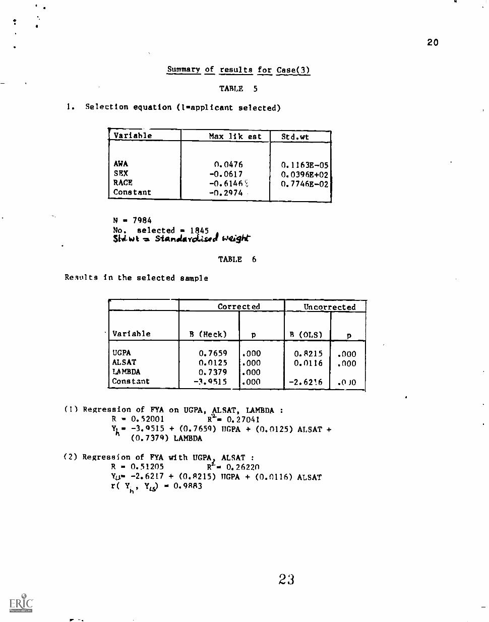
20

Summary of results for Case(3)

TABLE 5

1. Selection equation (1=applicant selected)

Variable Max lik est Std.wt

AWASEXRACEConstant

0.0476-0.0617-0.6146-0.2974

N = 7984No. selected = 1845Sivtlot s StitnoloYckiseer 64469hr

TABLE 6

Results in the selected sample

0.1163E-050.0396E+020.7746E-021

Corrected Uncorrected

Variable B (Heck) p B (OLS) p

UGPA 0.7659 .000 0.8215 .000ALSAT 0.0125 .000 0.0116 .000LAMBDA 0.7379 .000Constant -3.9515 .000 -2.6216 .0)0

(1) Regression of FYA on UGPA, ALSAT, LAMBDA :

R= 0.52001 R= 0.27041Yha -3.9515 + (0.7659) UGPA + (0.0125) ALSAT +

(0.7379) LAMBDA

(2) Regression of FYA with UGPA ALSAT :

R = 0.51205 RL= 0.26220Ya= -2.6217 + (0.8215) UGPA + (0.0116) ALSATr(Y,Yis) = 0.9883

23

21

Overall discuasion of all three cases:

In all three cases the difference in multiple R 's, with

Heckman's correction factor and with ordinary regression were

negligible. In case(2), because of selection on top of

selection, the variability of predictors was reduced very much

and so the R value is very small. In the other two cases,

although R values are quite significant, because of high

correlation between variables used as basis of selection and

also used as predictors in the subsequent regression, the

regression weights are very small.

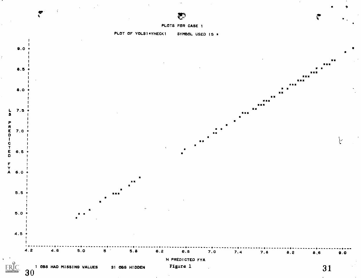
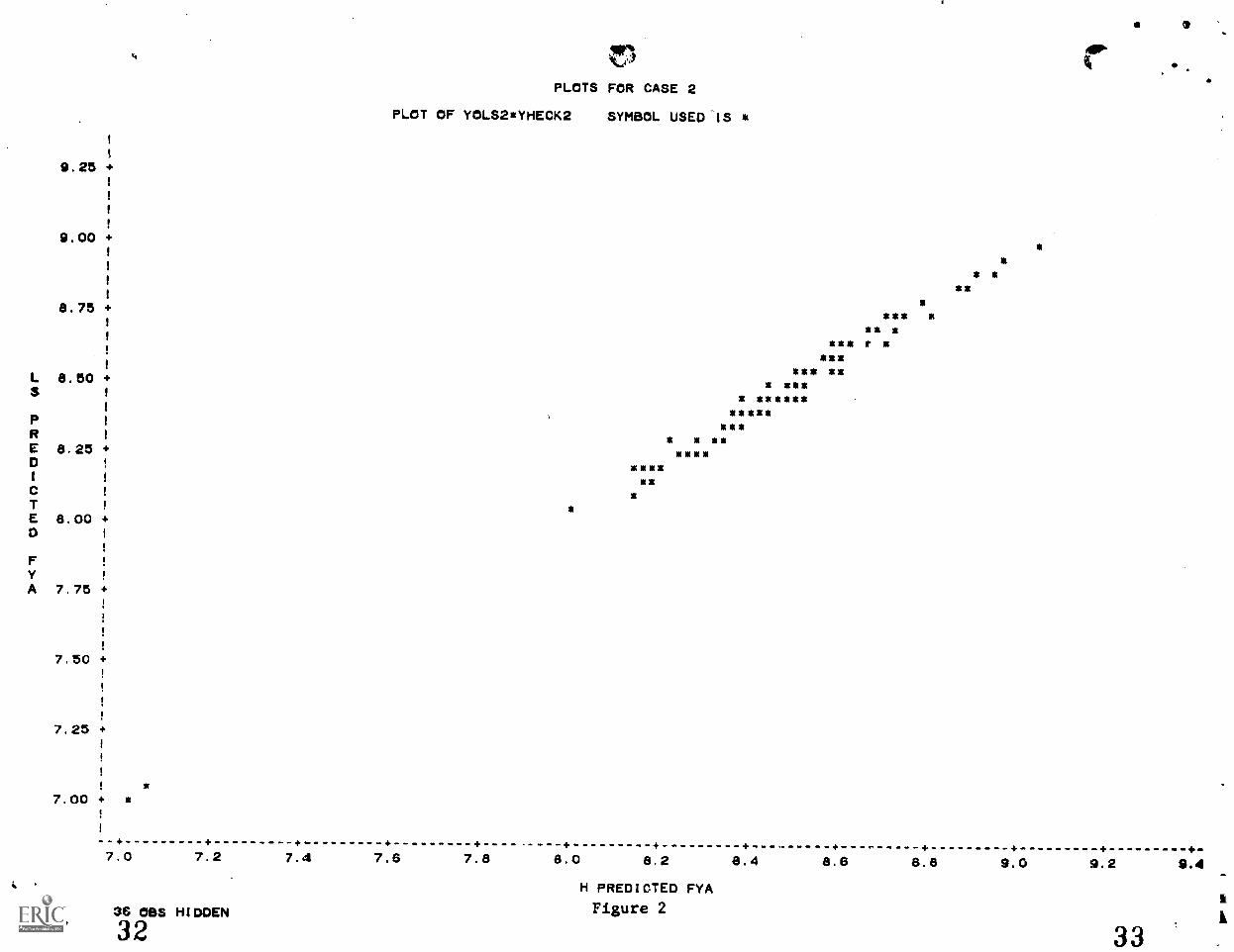
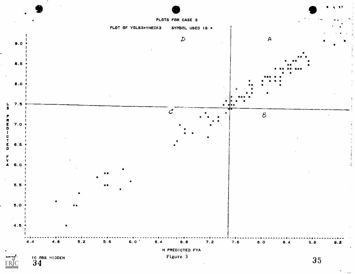
For all three of the above cases scatterplot of predicted

scores using correction factor "H predicted FYA" versus

predicted scores without the correction factor "LS predicted

FYA" are plotted in Figures (1), (2) and (3) for about 100

randomly chosen cases. As can he seen the two predicted values

are highly correlated in all the three cases, taking values

0.99, 0.83 and 0.99 respectively. So in this particular

situation, it would rarely make any difference which equation

is used for prediction purposes. However,it may make

difference which equation is used for prediction for particular

individuals. For example, if we consider the top 60 people for

selection, and set cut off lines as shown in Fig(3), it can

make a difference for the individuals in regions D and for one

individual in region B, which equation is used for selection.

24

22

Ordinary leastsquares equation rejects Individuals in region B

and accepts individuals in region D, whereas Heckman's

corrected regression equation rejects individuals in region D

and accepts individuals in region B.

23

Conclusion

The selection artifacts are pervasive in applied research.

Any data can be viewed as a selected subset from some larger

population. The solution of selection problems is based upon

the proper modelling, of the selection process. In situations

of explicit selection, under multivariate normality, results ofA

Goldberger (1981) can be used for correcting the selection

artifacts. Goldberger's results are robust when the assumption

of multivariate normality is not reasonable. In problems of

incidental selection there are no straightforward corrections

even under multivariate normality assumptions. The impact of

selection depends much upon the correlation between the error

terms in the two equation model. Berk, Ray and Cooley (1982)

note that correlations of near zero mean that incidental

selection effects are minor and correlations over .80 are

grounds for serious concern. Also there is the problem of

multicollinearity that can influence this correlation. It is

assumed that the errors In the two equations E and S have a

hivariate normal distribution. Alternatively one can assume a)

rectangular distribution, h) logistic distribution, c) errors

are linearly related. Again Berk, Ray and Cooley (1982)

conclude that it makes little difference in practice which of

the estimators one uses.

26

.t

24

In she foregoing discussion, the selectivity problem in

one group was considered. The method can be extended when

there are more than one nonequivalent groups. Muthen (1981)

has shown the statistical and computational ways of analyzing

selective samples by modeling the selection process in each

group. A simulation study by Muthen (1981) has been shown to

illustrate the failure of ANCOVA to show the significance of

the treatment effect in two groups due to selectivity problem.

In order to use Heckman's procedure for estimating the

unbiased estimates in selected samples the data requirement is

that the information on X used in Equation (3) be known for

the entire unrestricted sample. If the data is not available

on unselected applicant 'sample the method of estimating, the

unbiased parameters is given in Craig (1983). Research on the

violation of the assumption of bivariate normal distribution of

( and S is limited. Goldberger (1980) notes that when C

and are not bivariate normal, the results are biased but

less biased than when OLS is used ignoring the selection

process.

25

REFERENCES

Berk, R.A., Ray, S.C. & Cooley, T.F. Selection biases insociological data. Project Report, National Institute ofJustice (Grant No. 80-IJ-CX-0037). University of California,Santa Barbara, 1982.

Barnow, Burt s., Cain, Glen c., & Goldberger, Arthur S. Issuesin the analysis of selectivity bias.In Ernst W. Stromsdorferand George Farkas (Eds.), Evaluation Studies Review Annual ,

Vol. 5. Sage Publications: Beverly Hills/ London, 1980.

Bengt, M. and Joreskog, K. G. Selectivity problems in quasiexperimental studies. Paper presented for the conference onExperimental Research in Social Sciences ,Gainsville, Florida,January, 1981.

Dunbar, S. Corrections for sample selection bias. Ph.DThesis, 1982

Goldberger, A.S. Linear regression after selection. Journalof Econometrics ,1981, 15 , 357-366.

Gronau, R. Wage Comparisons - A selectivity bias. Journal ofPolitical Economy ,82 , 1119-1144, 1974.

Craig, A. Olsor and Brian, E. Becker. A proposed techniquefor the treatment of restriction of range in selelctionvalidation. Psychological Bulletin ,1983, 93 , 137-148

Heckman, J. J. Sample selection bias as a specificationerror. Econometrics ,1979, 47 ,153-161

Lewis, H. G. Comments on selectivity biases in wagecomparisions. Journal of Political Economy ,1145-1155,197H

Linn, R. L. Predictive bias as an artifact of selectionprocedure. Paper prepared for "Advances Psychometric Theory: AFestschrift for Frederic M. Lord," Princeton, NJ: EducationalTesting Service, May, 1982.

28

26

Tobin, J. Estimation of relationships for limited dependentvariables. econometrica , 1958, 26 , 24-36

Thorndike,R.L. Educational Measurement. American Council onEducation, Washington,D.C.,1971.

.1

V

9.0

8 . 5

+

+

PLOTS FOR CASE 1

PLOT OF YOLS1*YHECK1 SYMBOL USED IS *

X ****

*2**X*

***1

* *8.0 +IN*

**XX*

NC****L 7 . 5

S+

*

* **

*

*R 1

NC *E 7.0 +

*NC *

***

*E 6.5 + *0

A 6.0 +

** NC

*

*

5.5 + * * **

*

5.0 + * NI

*

4.5 +

4.2 4.6 5.0 5 5.8 6.2 6.6 7.0 7.4 7.8 8.2 8,6

H PREDICTED FYA

NOTE: 1 OBS HAD MISSING VALUES 31 OEM HIDDEN Figure 1

30

a

* *

31

+-9.0

9.25 +

PLOTS FOR CASE 2

PLOT OF YOLS2*YHECK2 SYMBOL USED IS *

9.00 +

** *

NC NC

8.75 + mom *

mg*** *r *

L3

8.50 +***

* ***

**amg

* **MX*mit

momR * * **E 8.25 + ****

****mg

E 8.00 +

0

A 7.75 +

7.50 +

7.25 +

*

7.00 + *

1

NOTE:f

7.0 7.2 7.4 7.6 7.8 8.0 8.2

36 OBS HIDDEN

32

H PREDICTED FYA

Figure 2

8.4 8.6 8.8

AP-r

9.0 9.2 9.4

33

PLOTS FOR CASE 3

9.0 +

PLOT OF YOLS3*YHECK3

8.5 +

8.0 4.

L 7.5

E 7.0 +

E 6.5 4.

A 6.0 +

a*

*5.5 + a*

5.0 + **

4.5 + *

SYMBOL USED IS a

** ** **

* ** ** **** *

*

**X ** * *

*** *

* *** ** a *

* **

.1* 8*

* *

4

-+ + + -- + + + , +4.4 4.8 5.2 5.6 6.0 6.4 6.8 7.2 7.6 8.0 8.4 S.8 9.2

NOTE: 10 OBS HIDDEN

34

H PREDICTED FYA

Figure 335