DOCUMENT RESUME

ED 064 357 TM 001 525

AUT4OR Kolakowski, Donald; Bock, R. DarrellTITLE Maximum Likelihood Estimation of Ability Under the

Normal Ogive Model; A Test of Validity and anEmpirical Example.

SPONS AGENCY National science Foundation, Washington, D.C.PUB DATE Apr 72NOTE 21p.; Paper presented at the annual meeting of the

American Educational Research Association (Chicago,Illinois, April 1972)

EDRS PRICE MF-$0.65 HC-$3.29DESCRIPTORS Ability Identification; *Guessing (Tests);

*Mathematical Models; *Measurement Instruments;Models; Psychometrics; *Statistical Studies; *TestResults; Test Validity

ABSTRACTThe estimation of values of a latent-trait presumed

to underlie a given set of item response data is made on the basis :)fdichotomously scored items utilizing the so-called Hnormal ogivemodelu of Lawley and Lord. This model provides an internal scale ofmeasurement, scores which are independent of the particular testitems employed, individual estimates of the standard error of eachsubject's score, and a statistical test of how well the data conformsto the constraints of the model. Tables and graphs present the studyresults. (Author/DB)

U.S. DEPARTMENT OF HEALTH.EOLTATION & WELFAREOFFICE OF EDUCATION

THIS DOCUMENT HAS BEEN REPRO-DUCED EXACTLY AS RECEIVED FROMTHE PERSON OR ORGANIZATION OMG-INATING IT. POINTS OF VIEW OR OPIN-IONS STATED DO NOT NECESSARILYREPRESENT OFFICIAL OFFICE OF EDUCATION POSITION OR POLICY.

MAXIMUM LIKELIHOOD ESTIMATION OF ABILITY

UNDER THE NORMAL OGIVE MODEL:

A TEST OF VALIDITY AND AN EMPIRICAL EXAMPLE.

Donald Kolakowski, University of Connecticut

R. Darrell Bock, University of Chicago

Paper presented at the anaual

American Educational ResearchChicago, April 3-7,

meeting of the

Association in1972.

This investigation was supported in part by National Science Foundation

Grant GJ-9 to the University of Connecticut Computer Center and NSF

Grant GS-1930 to the University of Chicago.

I. Introduction

Physical and physiological measurements are not generally subject to the

limitations inherent in psychological testing, where an unknown range of

individual variation is compressed into a relatively restricted distribution

of scores from a typically 10- to 40- item test. Such psychometric variables

produce raw scores distributions which tend to be skewed and platykurtic,

their particular properties being dependent upon the difficulty and discrim-

inating power of the test items employed (Lord & Novick, 1968, pp. 386-392).

To make valid inferences about the nature of these quantitative trwtts, especially-1

by means of distributional analyses, it is apparent that we need mental

variables possessing better metric properties than is usually the ease. A

theoretical solution for the hypothetical value of a trait or ability presumed

to underlie a given set of item-response data is provided by the latent-trait

pRychometric models (Lord & Novick, 1968, Chs. 16-20; Rasch 1960) In fhe present

study we consider the estimation of these trait values on the basis of n

dici,otomously-scored items utilizing the so-called "normal ogive model" of

Lawley and Lord (Lawley, 1943; Lord, 1952; Bock & Lieberman, 1970). This model

provides an internal scale of measurement, scores which are independent of the

particaar test items employed, individual estimates of the standard error of

each subject's score, and a statistical test of how well the data conforms

to the constraints of the model.

2

2. The Normal Ogive Model

Consider an unobservable, continuous variable, 0, the "latent ability"

of the subjects, which is distributed normally in the population of reference

with a mean 0.0 and variance 1.0. Letting rij=1 indicate a correct response

by subject i to a dichotomously scored item j, and rij=0 otLerwise, define

Prob frij

= (cj + aj 01.)

where 0 is the cumulative normal distribution function,

c is an index of the difficulty of item j

and aj is an index of the discriminating power of item j.

Then if ya = , the n x 1 score vector for a given subject, with

ability 0

(1)

n rijP ( vi ) = n Pij Qi (1 - rip, where Qij = 1 - (2)

J=1

on the assumption of "local independence "; ie that the probabilities

of a correct response to any two items for a given value of are

statistically independent of each other. (They are necessarily independent of

0 since 0 does not vary.)

A discussion of the plausibility of the normal ogive response character-

istic can be found in Lord and Novick (1968, Ch. 16). However, the adequacy

of the model must be verified for a given sample of test data. A common

situation in which one would not expect a good fit is that in which subjects

guess at unknown answers, thus raising the lower wymptotic value of

considerably above zero. Equation (1) is easily generalized to include

this possibility:

Pij = gj [1 - (cj + ai01)] 4. 0 (cj ajOi)

= gj + (1 - gj) 0 (cj + ajed

where gj is a constant specifying the probability of a chance correct

response to item j when 03 answer is unknown.

(3)

3

In general, the model requires that

(a) the test in question is measuriag substantially one trait (ie. a unifactor

test)

(b) the probability of answering a given item correctly increases monoton

ically with the subject's level on the trait, and

(c) the principle of local independence given above.

3. Maximum Likelihood Estimation of Latent Ability and Item Parameters

The estimation of the parameters of the model may be approached from an

unconditional or conditional point of view, depending .upon whether the subjects

are regarded as having been sampled from a specified population or are

treated as given entities (see Bock, 1972). The former approach has proven to

be extremely time consuming for tests of more than, say, ten items (Bock &

Lieberman, 1970). The latter leads to simultaneous estimation of both subject

and item parameters and has been adopted here because of its computational

efficiency.

A. Estimating ability when the item parameters are known

Letting the parameters of the model be defined as in section 2, and Pij

be defined by equation (3), P(..%) in equation (2) is the likelihood function of

0 for a giuen subject. Omitting the i and j subscripts for convenience,

= log P(v) = Er log P + E(1-r) log Q

Letting Yj Cj + ajO and h(Y) = the unit normal ordinate.

£(x Jar) 9P . EXZE a (1-g) h (Y) 0.az InPQ

90 P

(4)

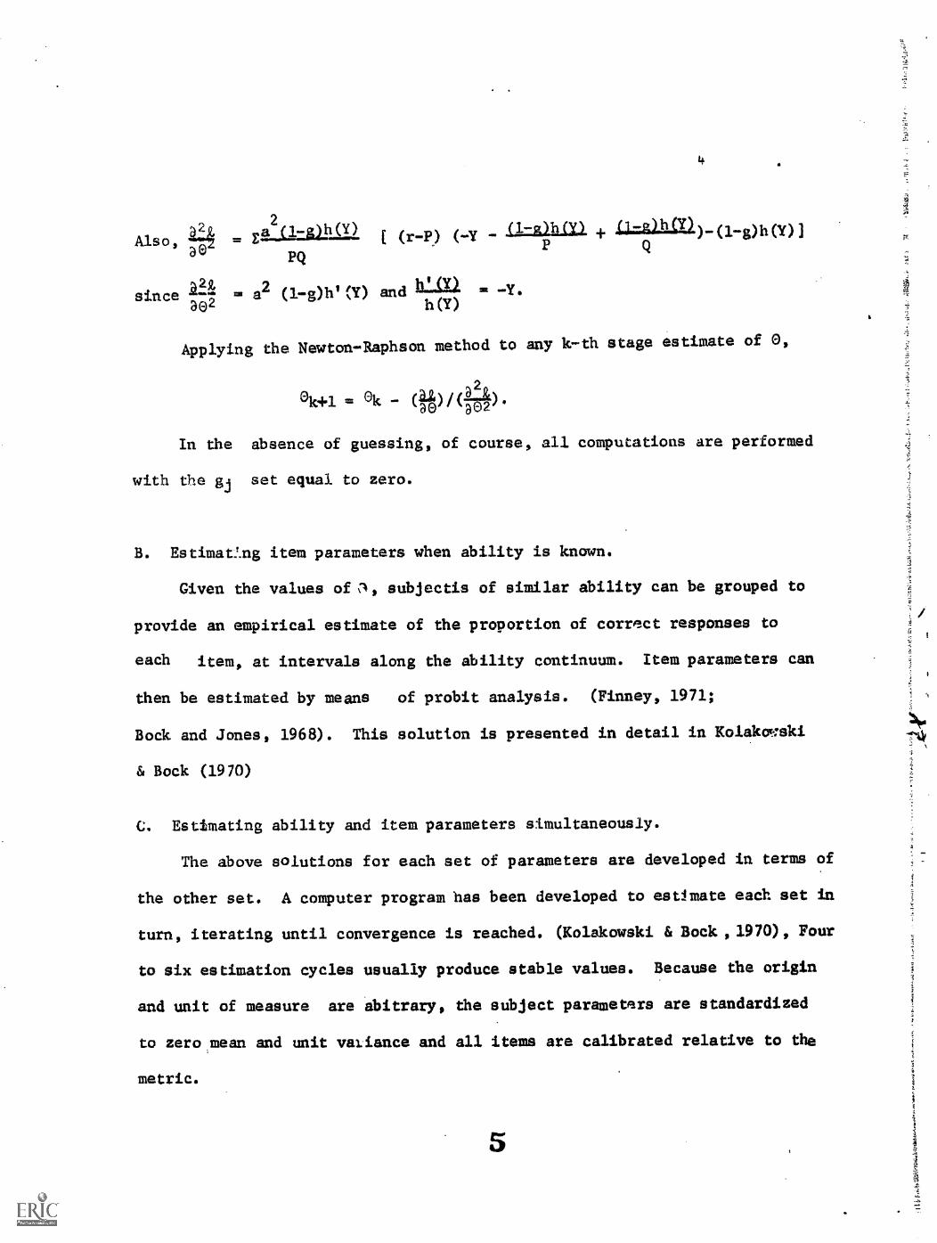
Also,

3".

4

2

0-12:$21111(2. [ (r-p) (1-011(y)

PQ

since = a2 (1-g)h(11) and W(Y)382 h (Y)

Applying the Newton-Raphson method to any k-th stage estimate of 0,

ek+1 =

In the absence of guessing, of course, all computations are performed

with the gj set equal to zero.

B. Estimat!mg item parameters when ability is known.

Given the values of subjectis of similar ability can be grouped to

provide an empirical estimate of the proportion of correct responses to

each item, at intervals along the ability continuum. Item parameters can

then be estimated by means of probit analysis. (Finney, 1971;

Bock and Jones, 1968). This solution is presented in detail in Kolakmski

& Bock (1970)

C. Estimating ability and item parameters simultaneously.

The above solutions for each set of parameters are developed in terms of

the other set. A computer program has been developed to estlmate each set in

turn, iterating until convergence is reached. (Kolakowski & Bock ,1970), Four

to six estimation cycles usually produce stable values. Because the origin

and unit of measure are abitrary, the subject parameters are standardized

to zero mean and unit valiance and all items are calibrated relative to the

metric.

5

The gj are presently treated as constants which must be determined by

inspectim. Subjects for whom the procedure will not converge are assigned

a default value and, in the present investigation, are eliminated from subsequent

analysis. The number of groups or fractiles used in partitioning the subjects

for the probit analysis is arbitrary.

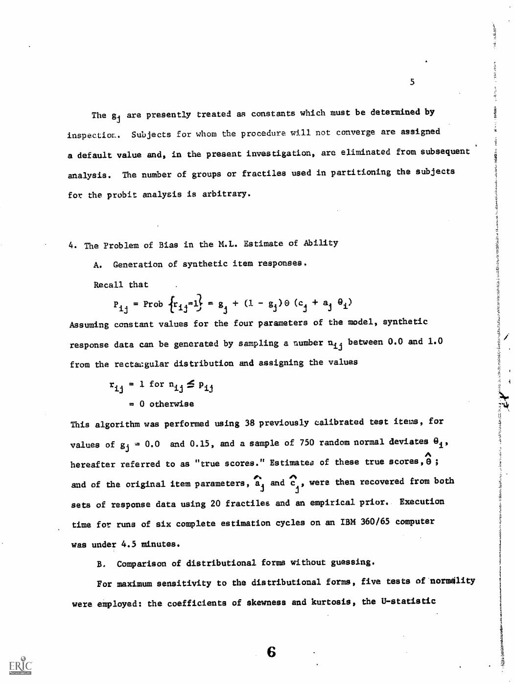
4. The Problem of Bias in the M.L. Estimate of Ability

A. Generation of synthetic item responses.

Recall that

j J

Assuming constant values for the four parameters of the model, synthetic

response data can be generated by sampling a number nij between 0.0 and 1.0

from the rectacgular distribution and assigning the values

rij

= 1 for n Acpij ij

= 0 otherwise

This algorithm WAS performed using 38 previously calibrated test items, for

values of gj = 0.0 and 0.15, and a sample of 750 random normal deviates

Ahereafter referred to as "true scores." Estimates of these true scores, ;

0%

and of the original item parameters a and c1

were then recovered from both4

J

sets of response data using 20 fractiles and an empirical prior. Execution

time for runs of six complete estimation cycles on an IBM 360/65 computer

was under 4.5 minutes.

B. Comparison of distributional forms without guessing.

For maximum sensitivity to the distributional forms, five tests of nom4lity

were employed: the coefficients of skewness and kurtosis, the U-statistic

= ratio of sample range to std. deli. (David et al , 1954), Geary's A =

ratio of mean deviation to std. dev. (Geary, 1947), and a Chi Square

test on 18 degrees of freedom. Table 1 presents these indices for the distribu-

tion of true scores and that of fhe resultant raw scores, thus illustrating

the unacceptable properties of the latter.

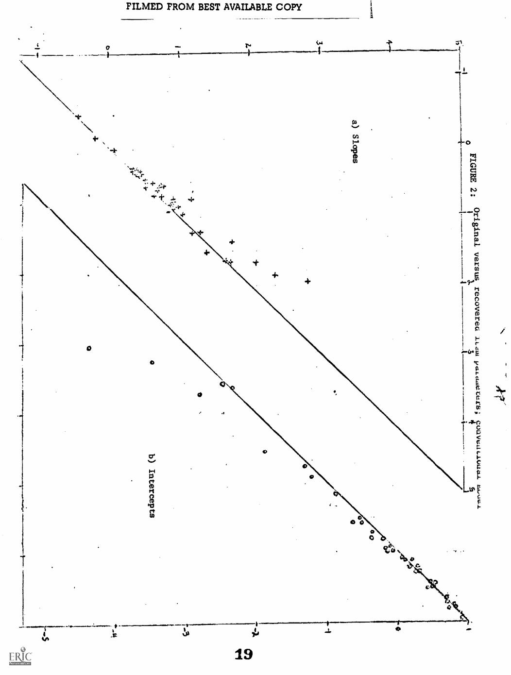
Table 2 (a) presents our results for the recovered estimates assuming the

gj = 0.0, ie. no chance responses. Although all of the sbility distributions

have a mean of zero and variance of one by constructioa, the form of the

distribution of the eiis leptokurtic and skewed to the right (Fig.1), indicating

that subjects of high ability receive inflated trait estimates. Thts is

explained by referring to fhe graph of original vs. recovered item parameters

(Figure 2), in which it is apparent that the easiest and most discriminating

items are estimated as being even more extreme, thus defining a lower bound

for ability, but having little weight in most calculations. On the other hand

A ethere is very little bias in the aj and cj of easy items. The net result is

a relative contraction of the left tail of the distribution.

A systematic correction for such asymmetrical bias is difficult to conceive.

However, the loss of a small number of unrealistically extreme subjects in the

context of a distributional analysis can be tolerated. Therefore since

there were no true scores beyond the range of approximately ± 3 standard

deviations, we accordingly removed the five subjedts whose trait estimates had

an absolute value greater than 3.0. Tabel 2(b) ahows that the distribution

of remaining subjects does not significantly differ from normality on any

of the five indices.

Similar analyses were performed for subtests of 10 and 20 items,

4:3

7

selected to uniformly span the entire range of difficulty. The program failed-

to converge to stable parameter estimates for a 10-item test. Apparently,

this is too few items to adequately describe an underlying normal distribution,

even with sudh a large number of subjects, and thus confirms the futility of

unconditional estimation with only a handful of items (see Bock, 1972).

The results for a 20-item test were similar to those for the 38 items

(Table 2(c)), with a stronger upward bias than was the case for the longer

test. Hence, the possibility exists that the use of large item pools could

itself improve the validity of ability estimates.

Given our priviledged knowledge of the true score distribution, the

original analysis was performed again assuming a normal prior rather than

the usual empirical prior. It can be seen in Table 2(d) that the results for

the two approaches are virtually identical. 'This is not surprising because,

whereas the normal prior fits the data more precisely, the extreme cases

(in both tails) are given considerably more weight than the moderate subjects.

Lastly, an analysis was performed assuming, contrary to fact, that the

fi subjects" might have been guessing. Here the procedure failed to converge

for each of three reasonable sets of guessing constants, each subjectively

determined from an examination of the item response proportions in the 20

fractiles. This tends to indicate that any results obtained under the guessing

model when this assumption is unwarranted will undoubtedly be invalid.

4

3

8

C. Comparison of distributions for data containing chance responses 8

The results of the analysis of the synthetic guessing data are presented

in Table 3 and Figure 3 for both the guessing and conventional options of the

computer nrogram. Whereas removing the extreme ui from these distributions

eliminated the original leptokurtosis, they remain significantly skewed to

the right although not nearly as extreme. Comparing the two response models in

Table 3 reveals that the guessing analysis is decided4 less skewed, and

therefore more valid, when chance responses are in fact present in the data.

However, the sensitivity of these tests will be better appreciated by referring

to Figure 3 for a subjective evaluation of the differences between models.

'11

'4

In conclusion, the normal ogive guessing model should be employed

when chance responses are likely to be present in the data, but failure of

the conventional model to converge for guessing data --and not vice versa--

indicates that the procedure will have the most validity in applications

where guessing can be ruled out. In any case, if the present methodology

is found to be valid for a variety of prior distributions, provision of

suitable default values for unrealistically high ability estimates and the

use of subjectively determined guessing constants might still allow generation

of pools of calibrated items and the implementation of sequential item

testing under consistent, if not ideal conditions.

5. Resolution of a Spatial Visualization trait distribution into normal components.

An empirical problem with data meeting the above ideal criteria involved

making an inference about the mode of inheritance of an educationally important

mental trait,spatial visualizing ability, by contrasting the properties of

the separate ability distributions for the sexes. A 29-item audio-visual

version of the Guilford-Zimmerman (1953) Spatial test was administered to

a sample of 727 eleventh-grade students. The Normal Ogive latent ability

estimates were obtained under the conventional model and the forms of the

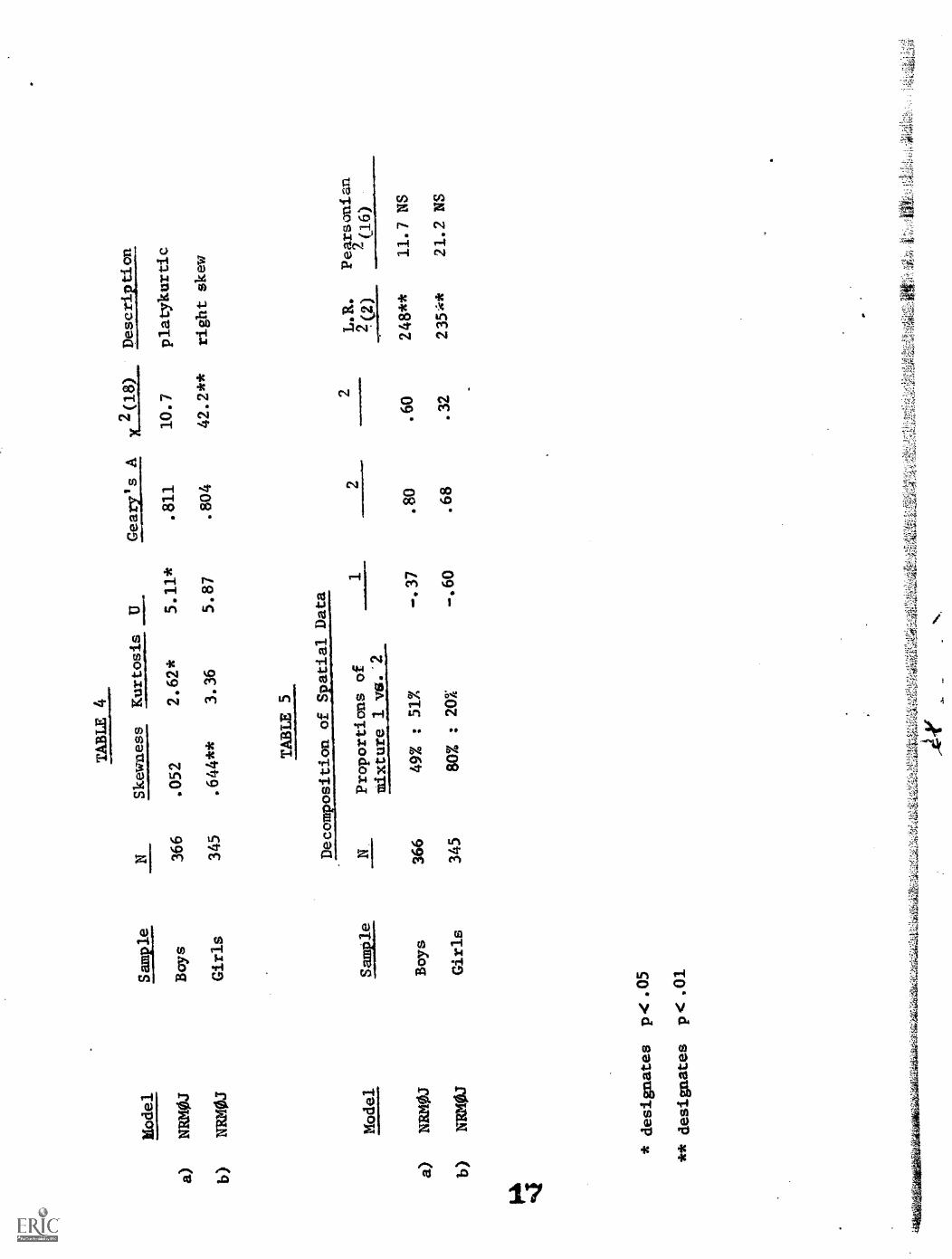
distributions were analysed for the sexes separately. Table.4 (a & b) shows

the results after removing extreme cases. Our first-hand knowledge of the data

plue the fact of convergence of the parameter estimates under the conventional

model, lead us to place considerable faith in the validity of this analysis.

A maximum likelihood decomposition of these distributions into normal

components by the method of Day (1969) yiteic: I.e results in Table 5 (a & b),

namely an upper component comprising 51% of tht: lariation in boys' spatial

10Th

10

ability which cc:responds to a similar component comprising only 20% of

the variance tor girls. Given ehe range of ability estimates from -2.0 to

+3.0, the means of .80 and .68 of these components, respectively, are virtually

equal. To deal objectively with the significance of the findings, a likelihood

ratio x2 test on 2 degrees of freedom was calculated to test the fit of only

one component. Also, a Pearsonian x2

on 16 degrees of freedom ws used to

check the adequacy of a bimodal model. These indices (Table 5) verified

that the deviation from normality shown in Table 4 is clue to the presence of

two and only two underlying components. This structure is illustrated in

Figure 3 against the background of the frequency histograms for the data.

The existence of a sex-differentiating duality in the distribution

of a continuous human variable is compelling evidence for a sex-influenced

major gene. The above proportions immediately suggest an X-linked recessive

allele with frequency close to 0.5. Moreover, the (assumed) common variance

of the components for girls is estimated at nearly one half the magnitude

of that for boys (Table 5), suggesting an averaging effect in females which

does not occur in males. This is entirely consistent with the hypothesis of

sex-linkage and decidedly reinforces the correlational evidence for this model.

(Stafford, 1961; Hartlage, 1970; Kolakowski, 1970)

6. Discussion'

While the importance of a latent-trait measurement model for validly

investigating the mode of inheritance of an intellectual ability is apparent,

it is equally clear that we need to be able to objectively select one of several

conflicting models without resort to considerations external to the estimation

problem. Internal corrections for bias and/or the simultaneous estimation of

guessing parameters for the Normal Ogive model are two as yet unrealized

approaches which would correct the weaknesses in the present investigation.

On the other hand, other psychometric models based upon the logistic distri-

bution may be more promising in this regard. (see Birnbaum, 1968; Basch,

1960).

For instances in which Chance responses can be eliminated on external

grounds, the assumption of normality of the components is still open to

scrutiny. Lord (1960) has shown that errors of measurement cannot be assumed

to be normally distributed if a subject's score is taLen to be the number

of items answered correctly. Latent traits being continuous and unbounded,

however, this assumption is at least plausible. It therefore remains to

investigate the bias of the foregoing procedures for a variety of true score

distributions or better yet, to specify theoretically the conditions under

which unbiased estimates can be expected to obtain.

12

References

Birnbaum, A. (1968) Some latent trait models and their use in inferring

an examinee's ability. Part V in Lord & Novick (1968) StatisticalTheories of Mental Test Scores below.

Bock, R.D. (1972) Estimating item parameters and latent ability when responses

are scored in two or more nominal categories. Psychometrika, 37; in press.

Bock, R.D. and Jones, L.V. (1968) The Measurement and Prediction of Judgement

and Choice. San Francisco: Holden Day.

Bock, R.D. and Lieberman, M. (1970) Fitting a response model for n dichotomously

scored items. Psychometrika,35; 179-197.

David, H.A., Hartley.H.O., and Pearson, E.S. (1954) the distribution

of the ratio, in a single normal sample, of range to standard deviation.

Biometrika, 41; 482-493.

Day, N.E. (1969) Estimating the components of a mixture of normal distributions.

Biometrika, 56; 463-474,

Finney, D.J. (1971) ProbitA. Cambridge University Press.

Geary, R.C. (1947) Testing for normality. Biometrika, 34; 209-242.

Guilford, J.P. and Zimmerman, W.F. (1953) Spatial visualization, form B.

Part VI of the Guilford-Zinmt.ititudeSurvarma. Beverly Hills:

Sheridan Supply Company.

Hartlage, L.C. (1970) Sex-linked inheritance of spatial ability. Perceptual

and Motor Skills, 31; 610.

Kolakowski,. D. (1970) A behavior-genetic analysis of spatial ability

utilizing latent-trait estimation. Unpublished Ph.D. dissertation,

Department of Education, University of Chicago.

Kolakowski, D. and Bock, R.D. (1970) A Fortran IV Program for maximumlikelihood item analysis and test scoring: Normal Ogive Model. Research

Memorandum No. 12, Educational Statistics Laboratory, University of Chicago.

Lawley, D.N. (1943) On problems connected with item selection and test

construction. Ltosseditaig, 61; 273-287.

Lord, P.M. (1952) A theory of test scores. Psychometric No.7.

Lord, F.M. (1960) An empirical study of the normality and independence

of errors of measurement in test scores. Psychometrika, 25e..91-104.

Lord, F.M. and Novick, M.R. (1968) Statistical Theories of Mental Test Scores.

Reading, Mass.: Addison-Wesley.

Er'N

="2-1

'';1

13

Rasch, G. (1960) Probabilistic Models for some Inte3_112.iencej_k_.,ndAttainment

Tests. Copenhagen: Danish Institute for Educational Research.

Stafford, R.E. (1961) Sex differences in spatial visualization as evidenceof sex-linked inheritance. Perceptual and Motor Skills, 13; 428.

14

CA

38 vocabulary items

TABLE 1

Randam data

750 subjects

Model

Sample

NSkewness

Furtosis

UGeary's A

x2(18)

Description

a)

True

scores

750

-.075

2.85

5.97

.802

12.5

b)

Raw

scores

750

-.399**

2.61**

4.97**

.812*

130**

left skew platykurtic

TABLE 2

a)

NRMOJ

rectangular

prior

Ability

estimate

749

.384**

4.20**

8.01**

.772**

27.2

right skew leptokurtic

b)

NRM0.1

rectangular

Ability

estimate:

744

.125

3.05

5.84

.791

14.6

prior

extremes

removed

c)

d)

NRMOJ

rectangular

prior

NRMOJ

20 items

Ability

745

.787**

4.79**

6.98

.756**

43.4**

right skew leptokurtic

normal

prior

estimate

749

.338**

4.18**

8.03**

.772**

21.7

right skew leptokurtic

* desigantes p<.05

** aesignates p.01

MIA 3

Nodel

Sample

Skewness

Kurtosis

Geary's A

x2(18)

a)

NRMOJ

Guessing

data

750

773**

4.02**

7.46*

.786

57.9**

b)

GUESS

Guessing

data

740

347**

3.62**

8.37**

.780**

32.7*

c)

NRMOJ

extremes

removed

Guessing

data

744

.507**

2.86

5.32*

.802

49.8**

d)

GUESS

extremes

removed

Guessing

data

737

.283**

2.94

5.63*(1)

.791

32.0*

*designates

p4.05

**designates p< .01

Description

right skew leptokurtic

right skew leptokurtic

right skew

right skew

TA

BL

E 4

Model

Sample

NSk

ewne

ssK

urto

sis

IIgm

alt..

...A

.x.

...{2

1$)

Des

crip

tion

a)N

RM

OJ

Boy

s

b)N

RM

OJ

Gir

ls

Mod

el

a)N

RM

OJ

b)N

RM

OJ

* de

sign

ates

p 4

.05

366

345

.052

.644

**

2.62

*

3. 3

6

5. 1

1*

5.87

.811

.80

4

10.

42.

TA

BL

E 5

7p

laty

kurt

ic

2**

righ

t ske

w

Dec

ompo

sitio

nof

Spa

tial D

ata

Prop

ortio

nsof

12

2L

. R.

Pear

s an

ian

mixture 1 vs.'2

(2)

2(1

6)

Boy

s36

649

%; 5

1737

.

Gir

ls34

580

% ;

20%

-.60

.

** designates

1)4.

01

80.6

024

8**

11. 7

NS

68.

3223

5;c*

21. 2

NS

,

A-7

coT-1

0

Scaled score

FIGURE 1: Distributionof recovered estimates

for the conventionalmodel

no.214

FIGURE 2:

Original versus recovereu

pc.Lciwecers; cuovaLiva4.1.

45

4

a) Slopes

4.

`

b) Intercepts

00

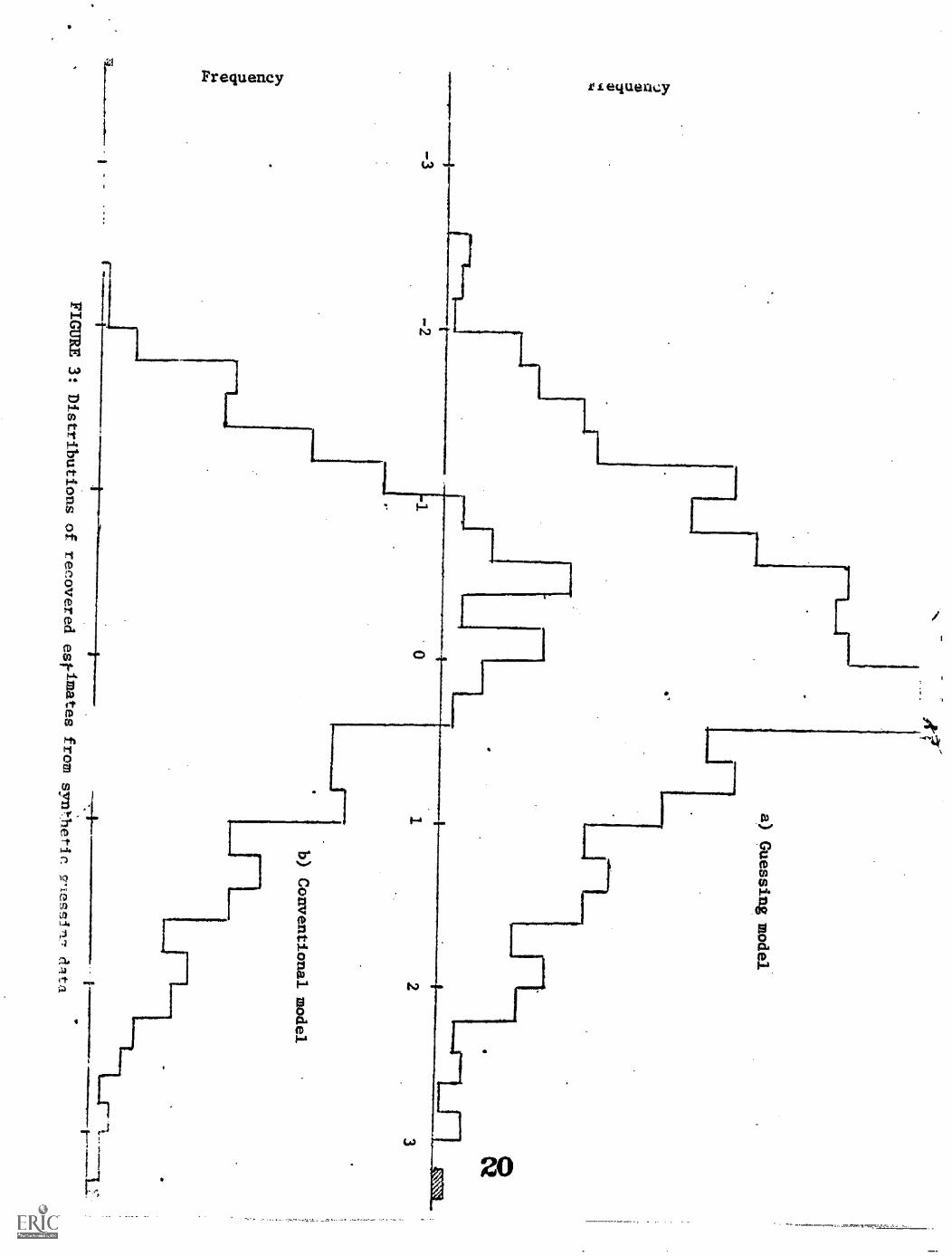
a) Guessing model

0C4

2

b) Conventional model

vimates from

syn1"betic

FIGURE 3: Distributions

of recovered

es

9-1e5sin-, dita

3

FIGU

RE

4 : SPAT

IAL

VISU

AL

IZA

TIO

NA

BIL

ITY

SCO

RE

DIST

RIB

UT

ION

S

BO

YS

.14=

380=

-.37m

2 =.80

a = .77

P1 =,.49

=1.7

df = 16

= 248.0

df = 2