Embed Size (px)
Citation preview

DOCUMENT
DE TRAVAIL
N° 329
DIRECTION GÉNÉRALE DES ÉTUDES ET DES RELATIONS INTERNATIONALES
GLOBAL IMBALANCES AND IMPORTED DISINFLATION IN THE EURO AREA
Jean Barthélemy and Guillaume Cléaud
June 2011
DIRECTION GÉNÉRALE DES ÉTUDES ET DES RELATIONS INTERNATIONALES
GLOBAL IMBALANCES AND IMPORTED DISINFLATION IN THE EURO AREA
Jean Barthélemy and Guillaume Cléaud
June 2011
Les Documents de travail reflètent les idées personnelles de leurs auteurs et n'expriment pas nécessairement la position de la Banque de France. Ce document est disponible sur le site internet de la Banque de France « www.banque-france.fr ». Working Papers reflect the opinions of the authors and do not necessarily express the views of the Banque de France. This document is available on the Banque de France Website “www.banque-france.fr”.
Global Imbalances and Imported Disinflation
in the Euro Area§
Jean Barthelemy∗ and Guillaume Cleaud∗
∗Banque de France - Monetary and Financial Research Department - Monetary PolicyResearch Unit§B. Saes-Escorbiac and J. Tanguy provided excellent research assistance. We thank L.
Benati, F. Bilbiie, F. Canova, R. Farmer, P.-O. Gourinchas, C. Hellwig, M. Juillard, S. Krause,M. Melitz, B. Mojon, R. Ranciere, S. Rebelo, J.P. Renne, A. Sbordone, and M. Woodford fortheir very helpful comments. We are also grateful for comments from seminar participants atthe Banque de France, INSEE and Universite de la Mediterranee Aix-Marseille 2. The viewsexpressed in this paper do not necessarily reflect the opinion of the Banque de France. Allremaining errors would be ours.Corresponding author : [email protected]
1
Resume
Nous estimons un modele DSGE pour la zone euro en economie ouverte. Le modele inclutdes tendances structurelles pour toutes les variables, ce qui nous permet de l’estimer en util-isant des donnees non filtrees. Dans un premier temps, nous derivons le sentier de croissanceequilibre compatible avec des chocs permanents de productivite, des changements de cibled’inflation et des modifications de long terme de l’ouverture des economies. Nous definissonsensuite le cycle comme l’ecart entre les donnees observees et cette trajectoire soutenable.Ainsi, notre modele peut integrer -sans manipulation prealable- les fluctuations de la balancecommerciale. Finalement, nous trouvons un effet persistent et important de l’augmentationdes imports relativement aux exports sur l’inflation de la zone euro sur les dix dernieres an-nees. Du premier trimestre 2000 au dernier trimestre 2008, nous estimons la contribution dudeveloppement desequilibre du commerce internationale sur l’inflation a hauteur de −0.7%et de −1.4% sur le taux d’interet nominal a 3 mois.
Code JEL: E32, F41.
Mots-cles: Desequilibres mondiaux, desinflation, cycle des affaires, macroeconomie eneconomie ouverte.
Abstract
We estimate a medium-scale DSGE model for the euro area in an open economy frame-work. The model includes structural trends on all variables, which allow us to estimate ongross data. We first provide a theoretical balanced growth path consistent with permanentproductivity shocks, inflation target changes, and permanent shocks to the openness of theeconomies. We then define the cycle as the gap between this sustainable trajectory and thegross data, thus our model properly deals with deviations of the trade balance. Finally, wefind persistent and strong effects from the asymmetric increase of euro area imports duringthe last ten years on domestic inflation. From the first quarter of 2000 to the last quarter of2008, we estimate the contribution of the imbalanced development of international trade oneuro area inflation to an average of −0.7%, and on the 3-Month interest rate to an averageof −1.4%.
JEL-code: E32, F41.
Keywords: Global Imbalances, Disinflation, Business Fluctuations, Open EconomyMacroeconomics.
2

1 Introduction
Global imbalances are considered as one of the main drivers of macroeconomic fluctuations, asemphasized by Obstfeld and Rogoff (2006), but few studies support the quantitative relevanceof this widespread idea. Indeed, business cycle models are often estimated after prefilteringdata ; consequently, in such models, persistent deviations of trade balance play little role inmacroeconomic fluctuations. To overcome that unwelcome feature, we suggest an assessmentof the importance of global imbalances through an estimation of trends and cycles in thesame framework following Barthelemy et al. (2009).
To assess evidence of imported disinflation due to global imbalances, we first define a bal-anced growth path which corresponds to the sustainable globalization path, then we analyzethe consequences of deviations from this balanced path, especially on inflation and interestrates. We estimate a two-country DSGE model for the euro area and the rest of the worldfrom 1985Q1 to 2009Q4 including five trends: two on productivity and inflation target inboth areas and one on the common movement of foreign biases which embodies the global-ization process. By introducing unit roots in our model, we are able to directly estimate ourmodel with non pre-filtered data. We find three main results.
First, we find a path consistent with the globalization process, permanent productivityshocks, and inflation target changes in both countries. To do so, we assume three hypotheses:a Cobb-Douglas aggregation of foreign and domestic goods in the utility function, the lawof one price in the long run, and a zero trade balance and net foreign asset position at longhorizon. In the spirit of King et al. (1988), who give restrictions on the utility functions toallow the existence of a balanced growth path, we prove that there exists a balanced growthpath if the ratio between the two countries’ foreign biases is expected to remain constantover time.
Second, the definition of a balanced growth path allows us to define economic-relevantcycles as the gap between gross data and this sustainable trajectory of the economy. So,we estimate a DSGE model with model-based long term fluctuations in the euro area andprovide a plausible decomposition between trends and cycles for all variables. We thencompare the stationary components we estimate to the standard HP-filtered variables, analyzetheir spectral decomposition, and confirm that, overall, our model-based cycles are botheconomically and statistically relevant.
Third, turning to the data, we find a strong deflationary effect of asymmetric globalizationsince 2000 for the euro area. From the first quarter of 2000 to the last quarter of 2008, weestimate the contribution of the imbalanced development of international trade on euro areainflation to an average of −0.7%. Without these persistent shocks affecting the euro areacurrent account, we find the Euribor-3M would have been 1.4 percentage points higher onaverage than it was during this period.
Global imbalances are one of the main topical issues in open macroeconomics. Obstfeldand Rogoff (2009) emphasize their role in the build up of the subprime crisis, but they remaina crucial issue even after the crisis and the considerable narrowing of the imbalances, asstressed by Blanchard and Milesi-Ferretti (2010). However, these concerns find few echoes inthe DSGE literature. Indeed, assessing the quantitative effects of global imbalances requiresa careful use of data.
Hence, as in the previous essay, we define model-based long term fluctuations by addingfirst order integrated shocks inside our DSGE model. Then we estimate at the same time thecyclical fluctuations and the trends generating process as suggested by Ferroni (2009). Asin Barthelemy et al. (2009), we include unit roots inside the model to reproduce long term
3

fluctuations of the data and estimate them simultaneously with the model’s deep parameters.The integration of non stationary shocks allows for a more economic definition of cycles thanstatistical filtering. Besides, it leads to the possible assessment of permanent shocks onthe cycle fluctuations. Finally, the assessment of global imbalances consequences cruciallydepends on how we define deviations from the sustainable path of globalization and thusneeds a precise assessment of globalization. In fact, previous open economy DSGE modelssuch as Adolfson et al. (2007) or Christoffel et al. (2008) detrend data so that trade balancefluctuations remain very small and weakly persistent, while our approach tends to be as closeas possible to the gross data. As an illustration, Figure 1 displays trade balance using HP-filtered data for exports and imports. This graph clearly exemplifies the need of a careful useof data as independent HP-filtering leads to errors in the sign, the size, and the persistenceof the trade balance.
Figure 1: EA Trade Balance over GDP ratio
One of the main features of globalization is the sharp increase of openness and we chooseto describe it as a shift in the demand for foreign goods. To determine the associated balancedgrowth path, we mainly make three assumptions: the aggregation of foreign and domesticgoods is a Cobb-Douglas function with a time-varying foreign bias, the law of one priceholds at long horizon to avoid long term deviations between domestic and export prices,and finally the trade balance and net foreign asset position are stationary with zero mean.Under these three assumptions we find that there exists a balanced growth path if the currentforeign biases ratio is equal to its expected value. We consider both permanent sustainableglobalization shocks and transitory shocks to the foreign biases. So, openness changes resultfrom the demand side, however it would have been strictly equivalent to include shifts intransport or barrier costs.
An outcome of our model-based trends and our estimated model is a strong and persistenteffect of asymmetric openness on output, inflation, and interest rates. This result stems from
4
a rather simple intuition that a country with an increasing propensity to consume foreigngoods rather than domestic ones undergoes deflationary pressures due to lower demand forits domestic goods. The imbalanced development of international trade contributed to anaverage of −0.7% on euro area inflation and of −1.4% on the 3-month interest rate, from2000 to 2008. Even if our propagation mechanism is quite intuitive, other papers emphasizeopposite effects from the imbalanced development of the international environment duringthe last decade. Some economists highlight the positive link between a foreign productivityshock and domestic inflation. Our model embodies this mechanism, but the direct effect ofsupply shocks in the rest of the world remains quite negligible, and the response of domes-tic inflation depends mostly on the resulting consumption profile. During the last decade,the extraordinary development of emerging economies, especially China, led to increasingdistortions between their national savings and their national investment. As a result, the dis-equilibrium caused by surplus countries generated disinflation and persistently low interestrates, as related by Macfarlane in a 2005 speech. Finally, Melitz (2003) shows that a demandfor a new variety coming from outward leads to more competitiveness, a fall in mark-ups andfinally a decrease in relative prices. Our model is unable to replicate Melitz’s result as weassume Dixit-Stiglitz aggregation hence, constant mark-ups. Nevertheless, we believe thatthe main impact of an increase in foreign production is a rise in inflation due to demandpressures on the capital and labor markets whereas Melitz assumes inelastic labor supply.
The remainder of this paper is organized as follows: section 2 brings some out-of-modelevidences of imported inflation due to global imbalances; section 3 details the main featuresof the model and the derivation of the balanced growth path consistent with both perma-nent openness changes; section 4 briefly describes the estimation procedure and the implieddecomposition; section 5 presents a quantitative assessment of the role of global imbalancesfor inflation in the Euro Area, while section 5 concludes.
2 Inflation and global imbalances: Some stylized facts
Trade balance disequilibrium is one of the key determinant of the so-called global imbalancesas they result in unbalanced net foreign asset position. Unbalanced trade may stem frommultiple reasons. One of the possible explanation that we are going to focus on is a transitorydisequilibrium between foreign demand of domestic goods and domestic demand of foreigngoods. This kind of disequilibrium may result from either an asymmetric change in tariffsor a change in the willingness to consume foreign goods. In both cases, this disequilibriumreflects a change in protectionism.
A transitory disequilibrium in external demands should have an impact on output-gapand therefore on inflation. Indeed, this disequilibrium should imply a lower demand for goodsproduced in the country with a deteriorating trade balance, and hence a fall in output-gap.In general equilibrium - i. e. if we assume that supply of production function inputs are notfixed - this decrease should trigger off a fall in wages and in the rate of return of capital andeventually a fall in GDP deflator inflation. Obviously, this mechanical presentation does notreflect the multiple other adjustments which can alter the link between distortions in externaldemands and inflation. Among others, monetary authority may raise its interest rate to limitthe magnitude of inflation change, exchange rate can adjust as the demand for each currencychange and so on.
Turning to international trade data, we find a positive link between inflation changes and
5

Figure 2: Correlations between inflation changes and trade balance over GDP changes.
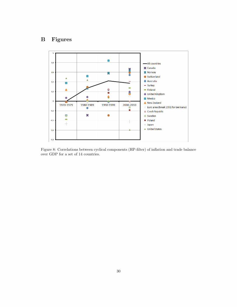
the trade balance changes for a set of 14 countries. We compute correlations between changesin inflation and the trade balance (in value and divided by GDP) for the last four decades ona quarterly basis. Figure 2 displays these correlations; each marker corresponds to a specificcountry whereas the black line stands for the overall correlation for all countries. The overallcorrelation rises from -0.06 for the seventies to 0.25 for the first decade of the century. Thispositive correlation (from 1980 and onwards) tends to support the idea that trade deficitleads to disinflation risk. In appendix, we check that this result remains when consideringHP-filtered data (see figure 8).
The positive correlation between inflation and the trade balance does not necessarily re-flect a causal relation, thus this positive correlation does not indicate the ”role” of globalimbalances for inflation. However, this stylized fact suggests that the mechanism we empha-size in this paper - i.e. a deteriorating trade balance due to a shift in demands for domesticgoods contributes negatively to the output-gap and the inflation - may be of first order mag-nitude. The remainder of this paper develops and estimates a two-country DSGE modelto test the quantitative relevance of trade disequilibrium for inflation and monetary policytaking into account key macroeconomic features relevant for this analysis.
3 The model
The model contains most of the standard key features of the recent literature in DSGE modelsin open economics. As in Christoffel et al. (2008), it includes monopolistic competition a laDixit-Stiglitz, with nominal rigidities on wages and prices a la Calvo, deep habits on domesticand foreign goods consumption, real rigidities on investment and a smoothed Taylor rule for
6

the interest rates. We build a model with a balanced growth path consistent with long termchanges in productivity, inflation target and openness by assuming three hypothesis: the con-sumer preferences over domestic and foreign goods are modeled as a Cobb-Douglas function;in the long run, producer pricing insures that the law of one price holds for both domesticand foreign goods; and the trade balance and net foreign asset position are stationary withzero mean.
This section begins with a general overview of the model, then describes the long termequilibrium path and finally discusses the sources of fluctuations.
3.1 General setup
We consider a two-country model in which households consume domestically produced goodsor imported goods, invest in domestically produced goods, rent their capital, adjust thecapital utilization rate and choose their wages as they propose a differentiated type of labor.A fraction of intermediary firms produce differentiated goods that they sell to final goodsproducers aimed at local market, while the rest of intermediary firms produce differentiatedgoods sold to exporters. In top of that, monetary policy adjust its nominal interest rateto limit unwelcome fluctuations and government authority decides their expenditures (indomestically produced goods).
Households
We assume a large number of identical households j ∈ [0, 1] maximizing their additive time-separable logarithmic utility function described by the following equation:
uj(t) = Et
[+∞∑T=t
β(T−t)eεBT
(lnCj,T −
L1+σlj,T
1 + σl
)](1)
where Et stands for the conditional expectation given information at time t, β denotesthe discount factor and σl is the inverse of the Frish elasticity of labor supply. Cj,T (resp.Lj,T ) is the overall utility-relevant consumption index (resp. hours worked) of household j attime T . Households face a trade-off between consuming domestic or foreign goods describedby a Cobb-Douglas aggregation function:
Cj,t =(CDj,t − hCDt−1)1−Ωt(Mj,t − hMt−1)Ωt[(
1− Ωt)(
1− he−gCD)]1−Ωt [Ωt(1− he−gM )]Ωt (2)
where CD (resp. M) corresponds to consumption in domestic (resp. foreign) goods, Ω isthe foreign bias (1 − Ω is the home bias), h is the deep external habit formation parameterand gX (resp. X) is the growth rate of the deterministic drift (resp. the balanced growthpath) of X. The assumption of Cobb-Douglas preferences over domestic and foreign goodsforces the price elasticity of imports to 1. However, recent studies, such as Imbs and Mejean(2009), argue that this elasticity might be much larger than 1. In the literature, the standardassumption on preferences is a CES function, which allows a greater price elasticity, asin Obstfeld and Rogoff (2006). Nevertheless, dealing with trends and keeping our modeltractable force us to choose this more specific form of utility. This simplification allows foran elegant solution to the balanced globalization path and facilitates the log-linearizationof our model around this equilibrium path. We assume deep habit formations on domesticgoods and imported goods to reduce the instantaneous response of imports and consumption
7

to a change of relative imports prices. Finally, the denominator of equation (2) correspondsto a normalization terms aimed at simplifying the log-linearization of such expression.
Households maximize their inter-temporal utility, equation (1), under the following budgetconstraint :
PCt Cj,t + PtIj,t + Tt + Ψ(zj,t)Kj,t−1 +Bj,t +BFj,tSt
(3)
= Wj,tLj,t + rkt zj,tKj,t−1 +Dt + ℵj,t +Rt−1Bj,t−1 +RBt−1B
Ft−1
St
where Tt denotes lump-sum taxes paid to the fiscal authority, zj,t the variable capitalutilization rate, Ψ(z) is the cost of the capital utilization (Ψ(1) = 0), Kj,t−1 the stock ofcapital, Bj,t domestic bonds, BFj,t foreign bonds, costing one unit of foreign currency todayfor RBt units of currency tomorrow, rkt the return on capital, Dt dividends and ℵj,t state-contigent securities providing insurance against household-specific wage-income risk.
Moreover, households own the capital Kj,t−1, rent a fraction zj,t to the firms, and investIj,t for the following periods, under the capital accumulation constraint, as in Christiano etal. (2005):
Kj,t = (1− τ)Kj,t−1 + (1 + εIt )(
1− S(
Ij,tIj,t−1
))Ij,t (4)
where S(ea) = S′(ea) = 0 and S′′(ea) = φ−1i is the real rigidities on investment parameter,
τ is the rate of depreciation of installed capital and εIt is an investment specific technologyshock affecting the efficiency of the newly installed investment good. Finally, households aresubject to nominal rigidities a la Calvo in their wage setting. At each period, a fraction ξwof the households is unable to re-optimize over its wage. Its wage Wj,t is then automaticallyindexed according to current productivity growth, current and past inflation target andprevious period consumer price inflation :
Wj,t =AtAt−1
(ΠPt
)1−γw(ΠPt−1π
Ct−1
)γwWj,t−1 (5)
where At, ΠPt and πC are productivity trend, inflation target and stationarized consumer
price inflation respectively, and γw is the weight of wage indexation on past consumer priceinflation. This indexation adapts the standard wage indexation equation to the context inwhich domestic GDP deflator inflation and consumer price inflation do not have the samesteady state. It insures a perfect indexation of all wages to the wage trend W = AP .Households resetting their wages fix their wages to maximize their utility function facing aspecific demand of labor due to an imperfect competition on labor market.
Firms
We assume a large number of identical firms, with a two factor production function, whereAt is the first order integrated productivity process, z is the capacity utilization rate, K isthe capital stock and L is labor.
Yt = (ztKt−1)α(AtLt)1−α (6)
where Lt is defined as :
8

Lt =(∫ 1
0
L1
1+λw,tj,t dj
)1+λw,t
(7)
where 1+λw,tλw,t
is the possibly time-varying wage elasticity of differentiated labor demand.A fraction of domestic intermediate firms sells their output Hi domestically, in monopolisticcompetition a la Dixit-Stiglitz:
Ht =(∫ 1
0
H1
1+λp,ti,t di
)1+λp,t
(8)
where 1+λp,tλp,t
is the possibly time-varying price elasticity of domestic goods demand. The
remainder of the domestic firms sell their output Xi overseas, facing the price elasticity 1+λXp,tλXp,t
.
In both markets, there is sluggish price adjustment due to staggered price contracts a laCalvo. Accordingly, a firm receives permission to optimally reset prices in a given period teither with probability 1− ξp or with probability 1− ξXp , depending on whether the firm sellsits differentiated output in the domestic or the foreign market. Prices which were not re-optimized are indexed on a weighted average of the current inflation target and the previousperiod domestic inflation:
Pi,t =(ΠPt−1
)γp(ΠPt
)1−γpPi,t−1 (9)
Fiscal and monetary authorities
We slightly modify a standard Taylor rule to take into account a potential use of both GDPdeflator inflation and HICP inflation. Furthermore, to avoid high frequency noises, we assumethat monetary authority reacts to year on year rather than quarterly data:
Rt = Rρt−1
(Rt
[(ΠPt,t−4
ΠPt
)θ(ΠCt,t−4
ΠCt
)1−θ]rπ[
Yte−4a
Yt−4
]ry)1−ρ
eεRt (10)
where ΠPt,t−4 and ΠC
t,t−4 are the quarterlized year on year GDP deflator and consumerprice inflation. ρ, θ, rπ and ry are the estimated parameters of the Taylor Rule. Here, ΠP isthe target of the central bank and is chosen exogenously, contrary to Ireland (2007)1.
The fiscal authority expenditures are simply represented by an exogenous AR(1) process.
Rest of the world
The modeling of the rest of the world in our model consists of a simplified symmetric versionof the domestic economy, excluding capital stock and investment from the economy. Besides,we assume a linear production function of foreign intermediate goods producers:
Y ∗t = A∗tL∗t (11)
1The balanced growth path for the consumer price inflation ΠC and the inflation target ΠP are relatedby the equation: ΠC = eΩ(gY −g∗Y )ΠP .
9

Trade balance and net foreign asset position
Equilibrium in the balance of payment occurs through purchasing or selling foreign bonds2
BFt , returning RBt units of foreign currency at date (t+ 1):
BFt = RBt−1BFt−1 +
(PXt Xt − StPMt Mt
)(12)
Where PX is the relative price of exported goods in domestic currency, PM the relativeprice of imported goods in foreign currency and S is the nominal effective exchange rate ofthe euro area in indirect quotation.
As in Schmidt-Grohe et al. (2003), we assume that the supply of foreign assets dependson the level of total assets to insure the stationarity of the net foreign asset position. Hence,there is a time-varying spread between the risk-free foreign interest rate and the interest ratefaced by the domestic country :
RBt = R∗t exp(−Φb
BFtPtYtSt
− εQt)
(13)
Where εQ is a shock on the external risk premium.
Market Clearing Conditions
The accounting equation for domestically produced goods gives the aggregate demand:
Yt = CDt + It +Gt +Xt (14)
where Y , CD, I, G and X correspond to total production, domestic goods consumption,investment, government expenditure and exports (in volume). Turning to the rest of theworld , the accounting equation is simpler:
Y ∗t = CD∗t +Mt (15)
3.2 Balanced growth path
In this section, we present the balanced growth path of the model. It consists of the equi-librium path of the considered macroeconomic variables, when neither transitory nor per-manent exogenous shocks hit the economy. As we allow unit roots, this balanced growthpath may change over time. We prove the existence of such a balanced growth path underthree assumptions: the consumer preferences over domestic and foreign goods are modeledas a Cobb-Douglas function; in the long run, producer pricing insures that the law of oneprice holds for both domestic and foreign goods; and the trade balance and net foreign assetposition are stationary with zero mean.
Main Hypothesis
First hypothesis: as we assume Cobb-Douglas preferences, the share of imports in theconsumption basket is exogenous and given by the foreign bias:
2In all subsequent sections, net foreign asset position will be only linearized, and not log-linearized, allowingboth positive and negative values, and a null steady state equilibrium value.
10

PtCDt1− Ωt
=PMtMt
Ωt= PCtCt (16)
Which results from maximization of equation (2).
Second hypothesis: assuming constant and equal long-term markup pricing on both do-mestic and foreign products, the law of one price holds along the balanced growth path forboth goods in our economy, as in Christoffel et al. (2008). Denoting by PX and PM , theprices of exports and imports, and by S the effective exchange rate of the euro area in indirectquotation, the following producer pricing equations thus hold in the long run:
PXt = StPt (17)P ∗t = StPMt (18)
Third hypothesis: we assume that the trade balance and the net foreign asset positionare null in the long run which find support in Figure 1. The latest assumption translates intothe following relation between exports and imports in value:
PXtXt = StPMtMt (19)
Real Effective Exchange Rate
We compute the long term equilibrium path of the real variables of the economy, using theaccounting equation (14):
Yt = CDt + It + Gt + Xt (20)
Along the balanced growth path, we assume that output, government expenditures, cap-ital stock, investment and wages grow at the same rate as productivity (following King etal., 1988). In the accounting equation for the domestically produced goods, if the share ofinvestment and government expenditures over total output remains constant over time, thenthe shares of final consumption goods production over output has also to remain constant.Let us denote this constant share by kC :
CDt + Xt = kC Yt (21)
Besides, using the fact that the trade balance must be zero along the equilibrium path,equation (19), in combination with equations (16) and (17):
(1− Ωt)Xt = ΩtCDt (22)
Hence, using equation (21): CDt = kC(1− Ωt)YtXt = kCΩtYt
(23)
11
Under our assumptions, the conditions leading to a sustainable balanced globalizationlead to a volume share of exports in final consumption goods production exactly equal to thevalue share of imports in the consumption basket.
Turning back to the hypothesis of a null trade balance at the equilibrium, equation (19),we obtain:
Ω∗t P∗CtC
∗t = StΩtPCtCt
St =Ω∗t P
∗CtC
∗t
ΩtPCtCt
Qt =Ω∗t C
∗t
ΩtCt(24)
The long-term real effective exchange rate Q, in indirect quotation, depends negativelyon the relative level of consumption, in conflict with Backus-Smith (1993). Furthermore, ourmodel predicts that, in the long run, the real exchange rate should depreciate when produc-tivity increases, contrary to models including Balassa-Samuelson effects. This contrastingprediction results from the monopolistic competition between goods, without any distinctionbetween tradable and non-tradable goods contrary to Burstein et al. (2006). Here, we followmost DSGE models in open economy framework. Finally, the long-term real exchange ratedepends -quite conventionally- negatively on the relative degree of openness.
A necessary condition for a balanced growth path
Along the balanced growth path, the no-arbitrage condition between holding domestic orforeign currency should hold:
Rt = R∗tEtStSt+1
(25)
where R and R∗ are the domestic and foreign nominal interest rates. Furthermore, firstorder conditions of the optimizing problems of households, equation (1), results in:
1 = Et
[Ct+1
Ct
C∗tC∗t+1
Qt+1
Qt
](26)
Which, using the expression of the long-term real effective exchange rate, equation (24),leads to:
Ω∗tΩt
= Et
[Ω∗t+1
Ωt+1
](27)
All in all, existence of a balanced growth path imposes a condition on the growth rate ofthe share of imported goods in the consumption basket. In other words, to get a balancedgrowth path consistent with openness trends requires that all countries open to internationaltrade at the same pace. A sufficient condition for the uncovered interest parity to hold inthe long run, in our model, is to impose that there exists a constant, kQ such that:
Ω∗t = kQΩt (28)
12

We will assume that equation 28 holds for the remainder of the analysis. It allows, in avery simple and tractable way, a sustainable permanent growth in international trade alongthe equilibrium path of the model. In what follows, we analyze the effects of transitorydeviations from the above described balanced globalization path.
3.3 Sources of fluctuations
We choose to include five underlying trends to fit almost all the long term movements andco-movements observed in the data.
We include two first order integrated process for domestic and foreign productivity, in or-der to meet the common trend in output, capital stock, investment, government expendituresand wages, in the two countries.
We also define two time-varying inflation targets to fit the progressive changes in thedomestic and foreign monetary rules during and before the ‘Great Moderation’ followingIreland (2007) and Feve et al. (2008). For instance, from 1990 to the introduction of theeuro in 1999, average inflation decreased from more than 6% to 1.8% in the euro area. Wefit this structural break through a first order integrated inflation target chosen by the centralbank. Furthermore, in our setup we allow the foreign and domestic inflation targets to differpermanently as there is no reason to assume the same process in the two zones.
Last but not least, we introduce a fifth first order integrated process, which we call theglobalization process, allowing the description of the considerable expansion in internationaltrade during the last twenty years.
Fluctuations of the openness
The trend of the domestic foreign bias, Ωt, is a non-stationary process bounded between 0and 1. We define it such that:
Ωt1− Ωt
=Ωt−1
1− Ωt−1eω+εΩt (29)
where ω is the steady state globalization drift and εΩt is the permanent globalization
innovation shock. We define Ω∗t according to equation (28) to warrant the existence of abalanced growth path.
Due to our assumption of a null long-term trade balance, an asymmetric preference shockcan only be specified as a transitory shock. Hence, our model also includes a transitoryglobalization process εγt , and a transitory asymmetric preference shock εδt , both following afirst order autoregressive process. Thus, the foreign biases are defined as:
Ωt = Ωt(1 + εγt + εδt )
Ω∗t = kQΩt(1 + εγt − εδt )(30)
It is this last transitory shock affecting foreign biases in an unsustainable manner thatwill be of particular interest for our analysis of the effect of global imbalances.
Shocks
Our model features 18 structural shocks:
13

• including five permanent shocks : domestic and foreign permanent productivity shocksεA and εA
∗, domestic and foreign inflation target shocks εΠ and εΠ∗ , the globalization
trend εΩ
• and thirteen transitory shocks matching the short term fluctuations of the thirteen ob-servable variables of our model: domestic and foreign preference shocks εB and εB
∗,
investment shock εI , government expenditures shock εG, wage shock εW , domestic andforeign cost push shocks εP and εP
∗, imports price shock εM , domestic and foreign in-
terest rate shocks εR and εR∗, external risk premium shock εQ, transitory globalization
shock εγ and transitory asymmetric preference shock εδ.
The permanent shocks on openness and on inflation targets are white noises, while theother shocks follow AR(1) processes. Standard errors of the innovations as well as the per-sistence of the shocks are estimated along with the structural parameters of the model.
4 Bayesian Inference
We estimate the model using Dynare on gross data for the euro area and the rest of the worldfrom the first quarter of 1985 to the last quarter of 2009. We first present the methodology forthis estimation. Then, we verify the economic and statistical relevance of the de-trended vari-ables of our model, and compare the cycles we obtain to those obtained through traditionalHP-filtering.
4.1 Estimation
Data
We use seasonally adjusted quarterly data from three databases, for the period comprising1985Q1 to 2009Q4.
Euro Area data prior to the last quarter of 2001 are extracted from the AWM database,created by Fagan et al. (2005) : GDP, private consumption, investment, compensationto employees, total employment, labor force, GDP deflator, HICP, short-term interest rate,nominal effective exchange rate, exports, and imports. From the first quarter of 2002 onwards,we complete this database with the corresponding Eurostat series, ECB data for short-terminterest rates and nominal effective exchange rate, and OECD data for Euro Area exports,imports, and harmonized unemployment rate. For the rest of the world, we use OECD datafor GDP and GDP deflator, as well as federal reserve interest rate.
We slightly transform this data to estimate our DSGE model by using model consistentstationary data. However, this transformation causes no information loss contrary to standardstatistical filters. In fact we mainly use first difference data and ratios rather than levels forinput data. Table 1 recaps the definition of data used for estimating our DSGE model.
Then the relations between input data and the variables of the model are straightforward.However, our model is not able to reproduce two long term fluctuations. These two trendsconcern the government expenditures which has grown with a larger rhythm than the pro-ductivity and the real wage which has decreased compared to GDP. To completely bridge thegap between data facts and our model properties, we need to add two ad hoc deterministictrends without deep microeconomic justification.
14

data definitiondY Real GDPdC Private Consumption deflated by HICPdI Real InvestmentdW Real Compensation per Employee times Labor ForcedΠP GDP Deflator InflationdΠC HICP InflationdR Nominal Interest RatedQ Real Effective Exchange RatedXY Exports-over-GDP ratio in valuedMY Imports-over-GDP ratio in valuedY ∗ Foreign Real GDPdΠ∗ Foreign GDP Deflator InflationdR∗ Fed Funds Rate
Table 1: Definition of observable variables used to estimate the model. All variables aretaken in log first difference. Except for domestic consumption, we deflate real variables byGDP deflator.
Calibrations
We calibrate a few parameters for which data are not informative enough or for which wehave a very precise a priori. The details of the calibration are given in the table 2.
The euro area average ratio of imports over consumption is calibrated to 0.2. Consistentwith the fact that the euro area is four times smaller than the rest of the world, in terms ofGDP, the foreign openness is calibrated to 0.05 (we assume a symmetric openness weightedby the GDP of each area). Steady state GDP share of consumption kC and investment kIare calibrated to their average value over the sample. The Cobb-Douglas parameter α iscalibrated to the standard value of 0.34.
The households’ discount factor is calibrated to 0.999 corresponding to a steady statevalue of interest rate in the euro area of 4.37%, accounting for a 1.8% steady state for CPIinflation, a 2.17% steady state growth of consumption and a contribution from the discountrate of 0.4%. The inverse of the domestic and foreign Frish elasticities, σl and σ∗l , arecalibrated to 2, as in Christoffel et al (2008). The annual depreciation rate of fixed capitalis set to 10%. Relative convexity of the capital utilization cost and interest rate elasticity ofthe net foreign asset position are quite arbitrarily set to 0.2 and 0.001 respectively.
All steady-state mark-ups are calibrated to 0.1. Given we do not observe foreign wagesand export prices, we calibrate the parameters ξ∗w and ξXp of these two Calvo contracts tothe standard value of 0.75. The weight of foreign wage indexation on past CPI γ∗w is set to0.5, while the weight of export price indexation on past export price inflation is set to 0.15.
Finally, we fix the CPI inflation target in the euro area to 1.8% from 1999Q1 onwards.We calibrate the standard deviation of the domestic inflation target shock to its estimatedvalue on the subsample from 1985Q1 to 1998Q4 of 0.0908, to avoid any bias in its estimationover the whole sample. As written above, we set the persistence of the domestic and foreigninflation target shocks and of the globalization trend to 0.
15

Priors and Posteriors
The priors chosen for the estimated parameters are quite standard and follow Barthelemy(2009). The priors on standard deviations of shocks follow an inverse gamma distribution,as in Smets and Wouters (2007), with standard deviation set to infinity, so as to let theestimation procedure converge as freely as possible. The mean of the prior distribution isan adequately chosen scaling parameter. For the persistence of the shocks, we choose betadistributions, as in Smets and Wouters (2007).
Long-term growth parameters are also estimated during the procedure. Their priors aredefined as a normal distribution with mean and standard deviation equal to the measuredmean of the estimated growth rates in the data sample. Domestic and foreign deep-habitformation parameters, as well as prices and wages dynamics are estimated with beta distribu-tion, as in Smets and Wouters (2007). Finally, all parameters from the domestic and foreignTaylor rules are estimated with standard priors.
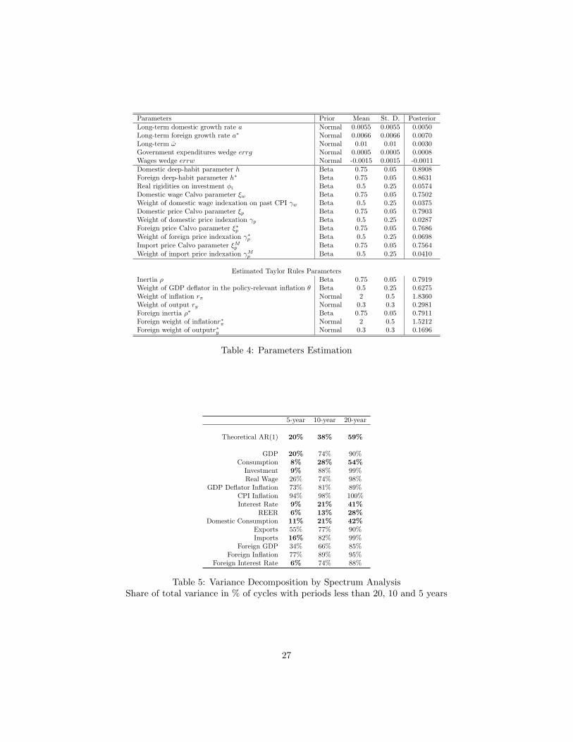
Tables 3 and 4 gather estimation results. First of all, contrary to standard findings in theliterature (Smets and Wouters (2007) for instance), the estimated persistence of all shocksbut the government expenditures shock ρG and the external risk premium shock ρQ arebelow 0.8, corresponding to a half-life of less than a year. The model describes very well thepropagation mechanism for most shocks, mitigating the need for high exogenous persistence.However, improvements have to be done in the understanding and modeling of fiscal policyand exchange rates. Estimation of the ‘taste and technology parameters’ remain very closeto standard estimates of the literature. Finally, the weight of GDP deflator inflation in theTaylor rule is of 63%, indicating a higher tendency of reacting to GDP deflator rather thanCPI inflation.
4.2 Sources of fluctuations
Figures 9 and 10 show the historical decomposition of GDP, consumption, investment, do-mestic consumption, exports, imports, GDP deflator and CPI inflation, and nominal interestrates. Each area corresponds to the contribution of a particular shock. So, if we add allthe shock’s contribution to the balanced growth path and the initial value of the endogenousvariable, we exactly fit the actual data. The structural decomposition of the cycle remainsvery similar to those found by Barthelemy et al. (2009) in closed economy. The business cycleremains mainly driven by domestic factors, in particular the government expenditures shockεG (hatched yellow), the investment shock εI (hatched sky blue), the domestic preferenceshock εB (dark blue), the permanent domestic productivity shock εA (hatched green) andthe domestic interest rate shock εR (orange).
The external risk premium shock εQ (dark grey) and the imports price shock εM (hatchedpink) have important consequences on consumption, investment, exports, imports and CPIinflation. However, their impact on overall GDP remains quite limited. The transitory skew-symmetric preference shock εδ (hatched brown) is one of the key determinants for explainingthe fluctuations of most macroeconomic variables. In particular, asymmetric developments ininternational trade since 2000 has contributed greatly to the low inflation pressures observedduring the last decade, and the particularly low nominal interest rates. But we will comeback to this core result later.
16
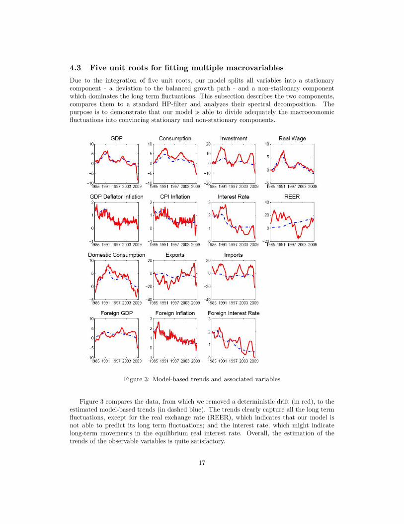
4.3 Five unit roots for fitting multiple macrovariables
Due to the integration of five unit roots, our model splits all variables into a stationarycomponent - a deviation to the balanced growth path - and a non-stationary componentwhich dominates the long term fluctuations. This subsection describes the two components,compares them to a standard HP-filter and analyzes their spectral decomposition. Thepurpose is to demonstrate that our model is able to divide adequately the macroeconomicfluctuations into convincing stationary and non-stationary components.
Figure 3: Model-based trends and associated variables
Figure 3 compares the data, from which we removed a deterministic drift (in red), to theestimated model-based trends (in dashed blue). The trends clearly capture all the long termfluctuations, except for the real exchange rate (REER), which indicates that our model isnot able to predict its long term fluctuations; and the interest rate, which might indicatelong-term movements in the equilibrium real interest rate. Overall, the estimation of thetrends of the observable variables is quite satisfactory.
17
Moreover, the trends are not simply a moving average or a band-pass filter. For instance,investment is above its trend from 2000 to 2008 while a moving average or a pass-bandfilter would have predicted cycles. Domestic consumption, exports, and imports also largelydeviate from their balanced growth path, corresponding to a deep global imbalances. Thispersistent change will be later related to the skew-symmetric shock on foreign biases whichexplains such disequilibria by an increase or a fall in the willingness to consume foreign goods.
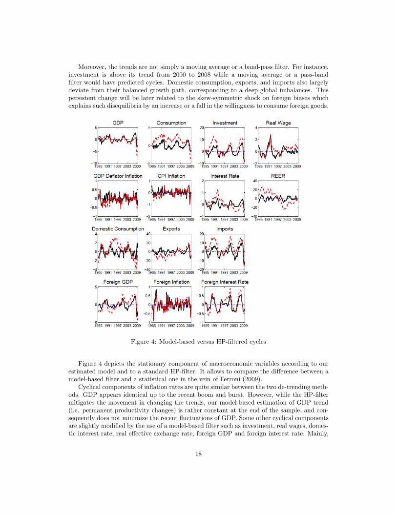
Figure 4: Model-based versus HP-filtered cycles
Figure 4 depicts the stationary component of macroeconomic variables according to ourestimated model and to a standard HP-filter. It allows to compare the difference between amodel-based filter and a statistical one in the vein of Ferroni (2009).
Cyclical components of inflation rates are quite similar between the two de-trending meth-ods. GDP appears identical up to the recent boom and burst. However, while the HP-filtermitigates the movement in changing the trends, our model-based estimation of GDP trend(i.e. permanent productivity changes) is rather constant at the end of the sample, and con-sequently does not minimize the recent fluctuations of GDP. Some other cyclical componentsare slightly modified by the use of a model-based filter such as investment, real wages, domes-tic interest rate, real effective exchange rate, foreign GDP and foreign interest rate. Mainly,
18

their volatilities are larger with our methodology compared to whose of HP-filter as HP-filteralways catch a part of large movements.
Finally, the choice of the methodology greatly modifies the identification of the stationarycomponents of domestic consumption, exports, and imports. These differences explain whywe need a model-based filtering to analyze global imbalances as HP-filter erases the persistentdeviations of these variables creating virtual cycles.
To test whether introducing five unit roots correctly reproduces the long term fluctuationsof the data in a more systematic and rigorous way, we decompose our model-based filtereddata through spectral analysis. Following Hamilton (1994), we first estimate an ARMA(8,8)process to fit our series and then compute the theoretical spectral analysis of such estimatedprocesses. We have to use high order lags and leads to ensure the theoretical autocorrelogramto fit the empirical one. We also compute the spectrum analysis of a first order autoregressiveprocess with a 0.9 persistence as a benchmark. Table A in Appendix reports the contributionof the cyclical components to the overall variance.
By construction, the HP-filter would give very good results by spectrum analysis as itselects the cycles with periods less than 8 years with the standard 1600 value for the smooth-ing parameter. However, our introduction of unit roots leads to stationary components ascyclical as an AR(1) process with 0.9 persistence. Exceptions are consumption and domes-tic consumption, the interest rate and the real effective exchange rate. The first two maystem from a slight change in the share of consumption over GDP that is not permitted bythe model. As for the domestic interest rate and the real effective exchange rate, the weakvariance due to short term cycles might indicate an incomplete modeling of their long-termtrends, as discussed above.
Overall, the spectral analysis confirms most of our model-based cycles are statisticallyrelevant. The decomposition of the observable in a trend and a stationary component seemsboth economically and statistically satisfactory.
5 Imported disinflation in the euro area
5.1 The skew-symmetric preference shock
Pre-filtering exports and imports separately prior to estimating the model, as is often donein the existing literature3, significantly reduces the importance of the skew-symmetric pref-erence shock. Nevertheless, thanks to our specification of the sustainable component of theglobalization process, we are able to isolate strong unsustainable deviations from the equi-librium path in the data. Consequently, our methodology contributes to rehabilitate theskew-symmetric shock on the trade balances, by inducing a higher estimated persistence andamplitude of this shock. We now focus on the effects of the transitory deviations of exportsand imports from their equilibrium path on the domestic and foreign economy.
We display the Impulse Response Functions to a skew-symmetric shock on foreign biases(εδt ) in Figure 5. When this shock is positive, it directly leads to an increase of importsand a fall in domestic consumption in value, by definition, and in volume as a result of slowand weak changes in relative prices. Conversely, as this shock is skew-symmetric, exportsdecrease and foreign domestic consumption increases. In the domestic country, as consumerslike more and more foreign goods, production decreases and thus leads to deflationary pres-sures in the domestic country. Consequently, monetary policy reacts in lowering its interest
3see Christoffel et al. (2008), Adolfson et al. (2007)
19
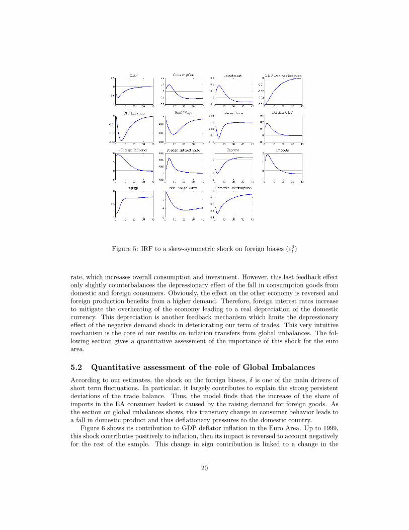
Figure 5: IRF to a skew-symmetric shock on foreign biases (εδt )
rate, which increases overall consumption and investment. However, this last feedback effectonly slightly counterbalances the depressionary effect of the fall in consumption goods fromdomestic and foreign consumers. Obviously, the effect on the other economy is reversed andforeign production benefits from a higher demand. Therefore, foreign interest rates increaseto mitigate the overheating of the economy leading to a real depreciation of the domesticcurrency. This depreciation is another feedback mechanism which limits the depressionaryeffect of the negative demand shock in deteriorating our term of trades. This very intuitivemechanism is the core of our results on inflation transfers from global imbalances. The fol-lowing section gives a quantitative assessment of the importance of this shock for the euroarea.
5.2 Quantitative assessment of the role of Global Imbalances
According to our estimates, the shock on the foreign biases, δ is one of the main drivers ofshort term fluctuations. In particular, it largely contributes to explain the strong persistentdeviations of the trade balance. Thus, the model finds that the increase of the share ofimports in the EA consumer basket is caused by the raising demand for foreign goods. Asthe section on global imbalances shows, this transitory change in consumer behavior leads toa fall in domestic product and thus deflationary pressures to the domestic country.
Figure 6 shows its contribution to GDP deflator inflation in the Euro Area. Up to 1999,this shock contributes positively to inflation, then its impact is reversed to account negativelyfor the rest of the sample. This change in sign contribution is linked to a change in the
20
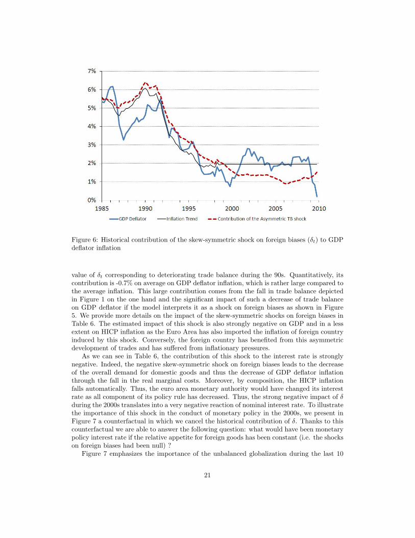
Figure 6: Historical contribution of the skew-symmetric shock on foreign biases (δt) to GDPdeflator inflation
value of δt corresponding to deteriorating trade balance during the 90s. Quantitatively, itscontribution is -0.7% on average on GDP deflator inflation, which is rather large compared tothe average inflation. This large contribution comes from the fall in trade balance depictedin Figure 1 on the one hand and the significant impact of such a decrease of trade balanceon GDP deflator if the model interprets it as a shock on foreign biases as shown in Figure5. We provide more details on the impact of the skew-symmetric shocks on foreign biases inTable 6. The estimated impact of this shock is also strongly negative on GDP and in a lessextent on HICP inflation as the Euro Area has also imported the inflation of foreign countryinduced by this shock. Conversely, the foreign country has benefited from this asymmetricdevelopment of trades and has suffered from inflationary pressures.
As we can see in Table 6, the contribution of this shock to the interest rate is stronglynegative. Indeed, the negative skew-symmetric shock on foreign biases leads to the decreaseof the overall demand for domestic goods and thus the decrease of GDP deflator inflationthrough the fall in the real marginal costs. Moreover, by composition, the HICP inflationfalls automatically. Thus, the euro area monetary authority would have changed its interestrate as all component of its policy rule has decreased. Thus, the strong negative impact of δduring the 2000s translates into a very negative reaction of nominal interest rate. To illustratethe importance of this shock in the conduct of monetary policy in the 2000s, we present inFigure 7 a counterfactual in which we cancel the historical contribution of δ. Thanks to thiscounterfactual we are able to answer the following question: what would have been monetarypolicy interest rate if the relative appetite for foreign goods has been constant (i.e. the shockson foreign biases had been null) ?
Figure 7 emphasizes the importance of the unbalanced globalization during the last 10
21

Figure 7: Counterfactual path of Nominal Interest Rate in absence of skew-symmetric shockson foreign biases (δt)
years on the monetary policy. It shows that if the euro area would have known a balancedopenness compared to the rest of the world, everything else being equal, the nominal interestrate would have been significantly higher (1.4 more in average from 2000 to 2008) and thuscloser to the neutral nominal interest rate. This quantitatively-relevant finding suggests thatglobal imbalances could have played a first role in the low rate/low inflation puzzle duringthe 2000s and finally partially confirms the intuition of Mac Farlane in his 2005 speech.
6 Conclusion
Economists often consider global imbalances as one of the main drivers of fluctuations andcrisis. However, because of methodological constraints this concerns find few echoes in quan-titative macroeconomic literature. We propose a simple way to include globalization processin order to assess the quantitative importance of persistent deviations to the associated bal-anced growth path. Thanks to the introduction of a non stationary component we are thusable to quantify the impact of deteriorating trade balance of the euro area since 1999.
We first derive a balanced growth path consistent with long term globalization, nonstationary productivity and inflation target under strong but standard assumptions. Thenwe provide evidence of the fit to data of our model in comparing stationary components toHP-filtered data and in proceeding in a spectrum analysis. Finally, we find evidence of astrong negative impact of unbalanced globalization on inflation and interest rates since 1999.According to our estimates, this latest result is one of the key ingredient which can explainthe low rate/low inflation puzzle of the mid 90s’.
22

To go one step further, these results emphasize the overall impact of global imbalances inthe economy and maybe one indirect explanation of the subprime crisis. Indeed our findingspartly explain the low nominal interest rates before the crisis which could have increasedthe risk taken by financial intermediaries as it is emphasized by Dubecq et al. (2009).Our microfoundation of the shock leading to such mechanism is however fragile and we donot argue that unbalanced globalization is only driven by shift in demand. Nevertheless, webelieve that the results would be the same in a model where the number of goods produced ineach country can fluctuate. In addition, our modeling of trade balance deviation is observablyequivalent to transport costs or trade tariffs such that we can interpret our results as a broaderanalysis of the consequences of unbalanced globalization with different sources. Because wethink of our shocks on foreign biases as a shortcut for supply and demand shocks whichlead to unbalanced globalization, we do not investigate the normative consequences of ouranalysis. Indeed, depending of the precise nature of the shocks the normative implication ofit would deeply change.
23
References
[1] Adolfson, M., S. Laseen, J. Linde, and M. Villani. “Bayesian Estimation of an OpenEconomy DSGE Model with Incomplete Pass-through”. Journal of International Eco-nomics, 72(2):481–511, 2007.
[2] Backus, D. K. and G. W. Smith. “Consumption and Real Exchange Rates in DynamicEconomies with Non-Traded Goods”. Journal of International Economics, 35(3-4):297–316, 1993.
[3] Barthelemy, J., M. Marx, and A. Poissonnier. “Trends and Cycles : an Historical Reviewof the Euro Area”. Documents de Travail 258, Banque de France, 2009.
[4] Blanchard, O. and G. M. Milesi-Ferretti. “Global Imbalances: In Midstream?” CEPRDiscussion Papers 7693, 2010.
[5] Burstein, A., M. Eichenbaum, and S. Rebelo. “The Importance of Nontradable Goods’Prices in Cyclical Real Exchange Rate Fluctuations”. Japan and the World Economy,18(3):247–253, 2006.
[6] Christiano, L., M. Eichenbaum, and C. L. Evans. “Nominal Rigidities and the DynamicEffects of a Shock to Monetary Policy”. Journal of Political Economy, 113(1):1–45,2005.
[7] Christoffel, K., G. Coenen, and A. Warne. “The New Area-Wide Model of the Euro Area- a Micro-Founded Open-Economy Model for Forecasting and Policy Analysis”. WorkingPaper Series 944, European Central Bank, 2008.
[8] Dubecq, S., B. Mojon, and X. Ragot. “Fuzzy Capital Requirements, Risk-Shifting andthe Risk Taking Channel of Monetary Policy”. Documents de Travail 254, Banque deFrance, 2009.
[9] Fagan, G., J. Henry, and R. Mestre. “An Area-Wide Model for the Euro Area”. EconomicModelling, 22(1):39–59, 2005.
[10] Ferroni, F. “Trend Agnostic One Step Estimation of DSGE Models”. MPRA Paper14550, University Library of Munich, Germany, 2009.
[11] Feve, P., J. Matheron, and J.-G. Sahuc. “Inflation Target Shocks and Monetary PolicyInertia in the Euro Area”. IDEI Working Papers 515, Institut d’Economie Industrielle(IDEI), Toulouse, 2008.
[12] Gorodnichenko, Y. and S. Ng. “Estimation of DSGE Models when the Data are Persis-tent”. Journal of Monetary Economics, 57(3):325–340, 2010.
[13] Hamilton, J. “Time Series Analysis”. Princeton University Press, 1994.
[14] Imbs, J. and I. Mejean. “Elasticity Optimism”. Working papers, HAL, 2009.
[15] Ireland, P. N. “Changes in the Federal Reserve’s Inflation Target: Causes and Conse-quences”. Journal of Money, Credit and Banking, 39(8):1851–1882, 2007.
24

[16] King, R. G., C. I. Plosser, and S. T. Rebelo. “Production, Growth and Business Cycles: I. The Basic Neoclassical Model”. Journal of Monetary Economics, 21(2-3):195–232,1988.
[17] Melitz, M. J. “The Impact of Trade on Intra-Industry Reallocations and AggregateIndustry Productivity”. Econometrica, 71(6):1695–1725, 2003.
[18] Obstfeld, M. and K. R. “Global Current Account Imbalances and Exchange Rate Ad-justments”. Brookings Papers on Economics Activity, 1:67–146, 2006.
[19] Obstfeld, M. and K. Rogoff. “Global Imbalances and the Financial Crisis: Products ofCommon Causes”. CEPR Discussion Papers 7606, 2009.
[20] Smets, F. and R. Wouters. “Shocks and Frictions in US Business Cycles: A BayesianDSGE Approach”. American Economic Review, 97(3):586–606, 2007.
A Tables
Parameters ValueDomestic openness Ω 0.2Foreign openness Ω∗ 0.05Domestic steady state GDP share of consumption kC 0.5736Domestic steady state GDP share of investment kI 0.2163Cobb-Douglas share of capital expenditure in total cost α 0.34Discount factor β 0.999Inverse of the domestic Frish elasticity σl 2Inverse of the foreign Frish elasticity σ∗l 2Depreciation rate τ 0.025Relative convexity of the capital utilization cost Ψ′′(1)
Ψ′(1) 0.2Interest rate elasticity of the net foreign asset position Φb 0.001Domestic wage mark-up λw 0.1Foreign wage mark-up λ∗w 0.1Domestic price mark-up λp 0.1Foreign price mark-up λ∗p 0.1Export price mark-up λXp 0.1Import price mark-up λMp 0.1Foreign wage Calvo parameter ξ∗w 0.75Weight of foreign wage indexation on past CPI γ∗w 0.5Export price Calvo parameter ξXp 0.75Weight of export price indexation γXp 0.15Domestic inflation target shock St. D. σΠ 0.0908Domestic inflation target shock persistence ρΠ 0Foreign inflation target shock persistence ρΠ∗ 0Globalization trend persistenceρΩ 0Domestic CPI inflation target ΠC 0.0045
Table 2: Parameters Calibration
25

Parameters Prior Mean St. D. Posterior
St. D. of shocksDomestic permanent productivity shock σA Inv. Gamma 0.5 +∞ 0.2201Foreign permanent productivity shock σA
∗Inv. Gamma 0.5 +∞ 0.2172
Foreign inflation target shock σΠ∗ Inv. Gamma 0.2 +∞ 0.0931Globalization trend σΩ Inv. Gamma 0.3 +∞ 0.1139Domestic preference shock σB Inv. Gamma 15 +∞ 4.6435Foreign preference shock σB
∗Inv. Gamma 15 +∞ 5.1665
Investment shock σI Inv. Gamma 50 +∞ 19.1523Government expenditures shock σG Inv. Gamma 5 +∞ 1.4252Wage shock σW Inv. Gamma 1 +∞ 0.3432Domestic cost push shock σP Inv. Gamma 0.5 +∞ 0.1874Foreign cost push shock σP
∗Inv. Gamma 0.5 +∞ 0.2493
Imports price shock σM Inv. Gamma 5 +∞ 1.3404Domestic interest rate shock σR Inv. Gamma 0.3 +∞ 0.1221Foreign interest rate shock σR
∗Inv. Gamma 0.3 +∞ 0.1080
External risk premium shock σQ Inv. Gamma 2 +∞ 0.4681Transitory globalization shock σγ Inv. Gamma 3 +∞ 1.2067Transitory skew-symmetric preference shock σδ Inv. Gamma 2 +∞ 0.7944
Persistence of shocksDomestic permanent productivity shock ρA Beta 0.75 0.05 0.7626Foreign permanent productivity shock ρA
∗Beta 0.75 0.05 0.7558
Domestic preference shock ρB Beta 0.5 0.25 0.2865Foreign preference shock ρB
∗Beta 0.5 0.25 0.6822
Investment shock ρI Beta 0.5 0.25 0.3834Government expenditures shock ρG Beta 0.5 0.25 0.9643Wage shock ρW Beta 0.5 0.25 0.0348Domestic cost push shock ρP Beta 0.25 0.05 0.2172Foreign cost push shock ρP
∗Beta 0.25 0.05 0.2227
Imports price shock ρM Beta 0.75 0.05 0.7613Domestic interest rate shock ρR Beta 0.5 0.25 0.6067Foreign interest rate shock ρR
∗Beta 0.5 0.25 0.5746
External risk premium shock ρQ Beta 0.5 0.25 0.9670Transitory globalization shock ργ Beta 0.5 0.25 0.4978Transitory skew-symmetric preference shock ρδ Beta 0.5 0.25 0.5520
Table 3: Parameters Estimation
26
Parameters Prior Mean St. D. PosteriorLong-term domestic growth rate a Normal 0.0055 0.0055 0.0050Long-term foreign growth rate a∗ Normal 0.0066 0.0066 0.0070Long-term ω Normal 0.01 0.01 0.0030Government expenditures wedge errg Normal 0.0005 0.0005 0.0008Wages wedge errw Normal -0.0015 0.0015 -0.0011Domestic deep-habit parameter h Beta 0.75 0.05 0.8908Foreign deep-habit parameter h∗ Beta 0.75 0.05 0.8631Real rigidities on investment φi Beta 0.5 0.25 0.0574Domestic wage Calvo parameter ξw Beta 0.75 0.05 0.7502Weight of domestic wage indexation on past CPI γw Beta 0.5 0.25 0.0375Domestic price Calvo parameter ξp Beta 0.75 0.05 0.7903Weight of domestic price indexation γp Beta 0.5 0.25 0.0287Foreign price Calvo parameter ξ∗p Beta 0.75 0.05 0.7686Weight of foreign price indexation γ∗p Beta 0.5 0.25 0.0698Import price Calvo parameter ξMp Beta 0.75 0.05 0.7564Weight of import price indexation γMp Beta 0.5 0.25 0.0410
Estimated Taylor Rules ParametersInertia ρ Beta 0.75 0.05 0.7919Weight of GDP deflator in the policy-relevant inflation θ Beta 0.5 0.25 0.6275Weight of inflation rπ Normal 2 0.5 1.8360Weight of output ry Normal 0.3 0.3 0.2981Foreign inertia ρ∗ Beta 0.75 0.05 0.7911Foreign weight of inflationr∗π Normal 2 0.5 1.5212Foreign weight of outputr∗y Normal 0.3 0.3 0.1696
Table 4: Parameters Estimation
5-year 10-year 20-year
Theoretical AR(1) 20% 38% 59%
GDP 20% 74% 90%Consumption 8% 28% 54%
Investment 9% 88% 99%Real Wage 26% 74% 98%
GDP Deflator Inflation 73% 81% 89%CPI Inflation 94% 98% 100%Interest Rate 9% 21% 41%
REER 6% 13% 28%Domestic Consumption 11% 21% 42%
Exports 55% 77% 90%Imports 16% 82% 99%
Foreign GDP 34% 66% 85%Foreign Inflation 77% 89% 95%
Foreign Interest Rate 6% 74% 88%
Table 5: Variance Decomposition by Spectrum AnalysisShare of total variance in % of cycles with periods less than 20, 10 and 5 years
27

1999 2000 2001 2002 2003 2004 2005 2006 2007 2008 2009Domestic
Output -1.2 -2.4 -2.0 -2.0 -1.9 -2.3 -3.3 -3.4 -2.8 -2.3 -1.3GDP defl. infl. -0.1 -0.5 -0.6 -0.6 -0.6 -0.6 -0.9 -1.0 -0.9 -0.8 -0.6
HICP infl. 0.1 -0.2 -0.5 -0.5 -0.5 -0.5 -0.6 -0.8 -0.8 -0.7 -0.6Interest Rates -0.7 -1.6 -1.2 -1.0 -1.0 -1.1 -1.8 -2.1 -1.4 -1.0 -0.7
ForeignOutput 0.5 0.8 0.6 0.6 0.6 0.6 0.9 0.9 0.7 0.6 0.3
GDP defl. infl. 0.0 0.1 0.2 0.2 0.2 0.2 0.2 0.3 0.2 0.2 0.1Interest Rates 0.1 0.3 0.3 0.2 0.2 0.3 0.4 0.5 0.3 0.2 0.2
Table 6: Yearly average contribution (in %) of the skew-symmetric preference shock εδt
28

εδεG
εIεB
εAεR
εQεB∗
εMεP
εγεP∗
othe
rsG
DPy
2818
199
612
11
11
10
4C
onsu
mpt
ionc
97
1115
74
351
110
00
1In
vest
men
ti
17
710
34
120
00
00
2R
eal
Wag
ew−p
12
330
272
20
013
00
20G
DP
Defl
ator
Infla
tion
π11
63
324
112
11
330
06
CP
IIn
flati
onπC
32
21
65
91
589
00
3In
tere
stR
ater
2614
139
315
32
41
10
10R
EE
Rq
122
20
02
721
40
00
4D
omes
tic
Con
sum
ptio
ncD
109
1513
104
50
00
270
7E
xpor
tsx
191
10
00
284
00
410
6Im
port
sm
170
01
00
270
160
320
7N
etFo
reig
nA
ssetb
270
01
00
702
00
00
0Fo
reig
nG
DPy∗
40
00
00
072
00
01
22Fo
reig
nIn
flati
onπ∗
10
00
00
028
00
057
14Fo
reig
nIn
tere
stR
ater∗
20
00
00
152
00
05
41
Obs
erva
bles
Rea
lG
DPdY
2231
2513
23
01
01
10
1P
riva
teC
onsu
mpt
ion
defla
ted
byH
ICPdC
22
176
34
50
60
00
1R
eal
Inve
stm
entdI
11
950
01
10
00
00
0R
eal
Com
pens
atio
npe
rE
mpl
oyee
tim
esL
abor
Forc
edW
00
10
150
00
024
00
59G
DP
Defl
ator
Infla
tion
dΠP
21
01
62
00
074
00
15H
ICP
Infla
tion
dΠC
00
00
12
60
6320
00
8N
omin
alIn
tere
stR
atedR
1913
128
134
01
32
10
6R
eal
Effe
ctiv
eE
xcha
nge
Eat
edQ
92
00
16
621
30
01
14E
xpor
ts-o
ver-
GD
Pra
tio
inva
luedX Y
47
32
03
303
00
400
7Im
port
s-ov
er-G
DP
rati
oin
valu
edM Y
354
20
00
30
220
310
2Fo
reig
nR
eal
GD
PdY∗
50
00
00
080
00
01
13Fo
reig
nG
DP
Defl
ator
Infla
tion
dΠ∗
00
00
00
04
00
088
9Fe
dFu
nds
Rat
edR∗
10
00
00
026
00
09
64
Oth
erV
aria
bles
ofIn
tere
stA
nnua
lG
DP
Gro
wth
3217
1711
87
01
11
10
3A
nnua
lC
onsu
mpt
ion
Gro
wth
43
247
76
131
150
00
2A
nnua
lG
DP
Defl
ator
Infla
tion
137
34
2913
31
112
00
13A
nnua
lH
ICP
Infla
tion
53
32
98
91
494
00
7
Tab
le7:
Var
ianc
eD
ecom
posi
tion
:ea
chnu
mbe
rco
rres
pond
sto
the
rela
tive
cont
ribu
tion
ofa
spec
ific
shoc
k(i
nco
lum
n)to
the
tota
lva
rian
ceof
apa
rtic
ular
vari
able
(in
line)
29
B Figures
Figure 8: Correlations between cyclical components (HP-filter) of inflation and trade balanceover GDP for a set of 14 countries.
30

Figure 9: Historical decomposition of main real variables
31

Figure 10: Historical decomposition of nominal variables
32

Documents de Travail
310. M. Crozet, I. Méjean et S. Zignago, “Plus grandes, plus fortes, plus loin…Les performances des firmes exportatrices françaises,” Décembre 2010
311. J. Coffinet, A. Pop and M. Tiesset, “Predicting financial distress in a high-stress financial world: the role of option prices as bank risk metrics,” Décembre 2010
312. J. Carluccio and T. Fally, “Global Sourcing under Imperfect Capital Markets,” January 2011
313. P. Della Corte, L. Sarnoz and G. Sestieri, “The Predictive Information Content of External Imbalances for Exchange Rate Returns: How Much Is It Worth?,” January 2011
314. S. Fei, “The confidence channel for the transmission of shocks,” January 2011
315. G. Cette, S. Chang and M. Konte, “The decreasing returns on working time: An empirical analysis on panel country data,” January 2011
316. J. Coffinet, V. Coudert, A. Pop and C. Pouvelle, “Two-Way Interplays between Capital Buffers, Credit and Output: Evidence from French Banks,” February 2011
317. G. Cette, N. Dromel, R. Lecat, and A-Ch. Paret, “Production factor returns: the role of factor utilisation,” February 2011
318. S. Malik and M. K Pitt, “Modelling Stochastic Volatility with Leverage and Jumps: A Simulated Maximum Likelihood Approach via Particle Filtering,” February 2011
319. M. Bussière, E. Pérez-Barreiro, R. Straub and D. Taglioni, “Protectionist Responses to the Crisis: Global Trends and Implications,” February 2011
320. S. Avouyi-Dovi and J-G. Sahuc, “On the welfare costs of misspecified monetary policy objectives,” February 2011
321. F. Bec, O. Bouabdallah and L. Ferrara, “the possible shapes of recoveries in Markof-switching models,” March 2011
322. R. Coulomb and F. Henriet, “Carbon price and optimal extraction of a polluting fossil fuel with restricted carbon capture,” March 2011
323. P. Angelini, L. Clerc, V. Cúrdia, L. Gambacorta, A. Gerali, A. Locarno, R. Motto, W. Roeger, S. Van den Heuvel and J. Vlček, “BASEL III: Long-term impact on economic performance and fluctuations,” March 2011
324. H. Dixon and H. Le Bihan, “Generalized Taylor and Generalized Calvo price and wage-setting: micro evidence with macro implications,” March 2011
325. L. Agnello and R. Sousa, “Can Fiscal Policy Stimulus Boost Economic Recovery?,” March 2011
326. C. Lopez and D. H. Papell, “Convergence of Euro Area Inflation Rates,” April 2011
327. R. Kraeussl and S. Krause, “Has Europe Been Catching Up? An Industry Level Analysis of Venture Capital Success over 1985-2009,” April 2011
328. Ph. Askenazy, A. Caldera, G. Gaulier and D. Irac, “Financial Constraints and Foreign Market Entries or Exits: Firm-Level Evidence from France,” April 2011
329. J.Barthélemy and G. Cléaud, “Global Imbalances and Imported Disinflation in the Euro Area,” June 2011
Pour accéder à la liste complète des Documents de Travail publiés par la Banque de France veuillez consulter le site : http://www.banque-france.fr/fr/publications/documents_de_travail/documents_de_travail_11.htm For a complete list of Working Papers published by the Banque de France, please visit the website: http://www.banque-france.fr/fr/publications/documents_de_travail/documents_de_travail_11.htm Pour tous commentaires ou demandes sur les Documents de Travail, contacter la bibliothèque de la Direction Générale des Études et des Relations Internationales à l'adresse suivante : For any comment or enquiries on the Working Papers, contact the library of the Directorate General Economics and International Relations at the following address : BANQUE DE FRANCE 49- 1404 Labolog 75049 Paris Cedex 01 tél : 0033 (0)1 42 97 77 24 ou 01 42 92 62 65 ou 48 90 ou 69 81 email : [email protected] [email protected] [email protected] [email protected] [email protected]