Doctoral Thesis

Detection of TeV gamma-raysfrom the Supernova Remnant RX J0852.0−4622

Hideaki Katagiri

Department of Physics, Graduate School of ScienceThe University of Tokyo

Hongo, Bunkyoku, Tokyo 113-0033, Japan

December 19, 2003

Abstract

Sub-TeV gamma-rays emitted from the northwest rim of the supernova remnant RXJ0852.0−4622 , where maximum non-thermal X-rays were detected by ASCA, were ob-served by the CANGAROO-II 10-m imaging air Cherenkov telescope (IACT) at SouthAustralia in 2002 and 2003. Data obtained in 187 hours of observation time gave the6.4 σ statistical significance using the image analysis with the likelihood method. Theflux of gamma-rays was 0.25 ± 0.06 times that of the Crab nebula at 500GeV with thespectral index of −4.5 ± 0.7 above 300GeV. The α (image orientation angle) distributionindicated a marginally extended emission, but was still consistent with a point sourcewithin statistical errors. The center of the obtained morphology coincided with the X-ray maximum point. The gamma-ray spectra were estimated under the assumptions ofthe synchrotron/inverse Compton model and decay of π0s produced by proton-nucleoncollisions. Our data strongly favored TeV gamma-ray emission from π0 decay. A totalcosmic-ray energy of 1048 to 1050 erg is required, when the molecular cloud density is5000 to 50 protons cm−3, assuming the distance was 0.5 kpc. The two-zone model of syn-chrotron/inverse Compton model with fine structures of X-ray emissions, however, canalso explain the broadband spectrum. Further observations and analyses such as XMM-Newton and Chandra X-ray satellites, NANTEN radio telescope, and CANGAROO-IIIstereoscopic system (IACTs) are strongly awaited to confirm the emission mechanism.

Contents

1 Introduction 8

2 Review 102.1 Origin of Cosmic Rays . . . . . . . . . . . . . . . . . . . . . . . . . . . . . 102.2 Fermi Acceleration . . . . . . . . . . . . . . . . . . . . . . . . . . . . . . . 142.3 Diffusive shock acceleration (DSA) . . . . . . . . . . . . . . . . . . . . . . 152.4 Observations of TeV gamma-rays from Supernova Remnants . . . . . . . . 182.5 SNR RX J0852.0−4622 (G266.2−1.2) . . . . . . . . . . . . . . . . . . . . . 242.6 Processes of Non-thermal Emissions . . . . . . . . . . . . . . . . . . . . . . 27

2.6.1 π0 decay . . . . . . . . . . . . . . . . . . . . . . . . . . . . . . . . . 272.6.2 Synchrotron Radiation . . . . . . . . . . . . . . . . . . . . . . . . . 272.6.3 Inverse Compton Scattering . . . . . . . . . . . . . . . . . . . . . . 282.6.4 Bremsstrahlung . . . . . . . . . . . . . . . . . . . . . . . . . . . . . 29

3 Imaging Air Cherenkov Technique 303.1 Overview . . . . . . . . . . . . . . . . . . . . . . . . . . . . . . . . . . . . . 303.2 Extensive Air Showers . . . . . . . . . . . . . . . . . . . . . . . . . . . . . 31

3.2.1 Electromagnetic Showers . . . . . . . . . . . . . . . . . . . . . . . . 313.2.2 Hadronic Showers . . . . . . . . . . . . . . . . . . . . . . . . . . . . 34

3.3 Cherenkov Radiation . . . . . . . . . . . . . . . . . . . . . . . . . . . . . . 373.4 Imaging Air Cherenkov Technique . . . . . . . . . . . . . . . . . . . . . . . 39

4 The CANGAROO-II 10-m Telescope 434.1 Reflector . . . . . . . . . . . . . . . . . . . . . . . . . . . . . . . . . . . . . 454.2 Imaging Camera . . . . . . . . . . . . . . . . . . . . . . . . . . . . . . . . 464.3 Electronics and Data Acquisition System . . . . . . . . . . . . . . . . . . . 48

5 Observations and Calibrations 525.1 Observations . . . . . . . . . . . . . . . . . . . . . . . . . . . . . . . . . . . 525.2 Calibrations . . . . . . . . . . . . . . . . . . . . . . . . . . . . . . . . . . . 52

5.2.1 Terminologies . . . . . . . . . . . . . . . . . . . . . . . . . . . . . . 535.2.2 Field Flattening . . . . . . . . . . . . . . . . . . . . . . . . . . . . . 535.2.3 Time-walk Corrections . . . . . . . . . . . . . . . . . . . . . . . . . 535.2.4 Rejection of Bad Channels . . . . . . . . . . . . . . . . . . . . . . . 535.2.5 DST10 . . . . . . . . . . . . . . . . . . . . . . . . . . . . . . . . . . 545.2.6 ADC Conversion Factor . . . . . . . . . . . . . . . . . . . . . . . . 54

1

6 Analysis 566.1 Reduction of the Night Sky Background (NSB) . . . . . . . . . . . . . . . 56

6.1.1 ADC Distributions . . . . . . . . . . . . . . . . . . . . . . . . . . . 566.1.2 Clustering . . . . . . . . . . . . . . . . . . . . . . . . . . . . . . . . 566.1.3 TDC Cut . . . . . . . . . . . . . . . . . . . . . . . . . . . . . . . . 56

6.2 Cloud Cut and Elevation Cut . . . . . . . . . . . . . . . . . . . . . . . . . 586.3 Selection of Bad Pixels due to Starlights and Electrical Noises . . . . . . . 606.4 Selection of Bad Pixels using ADC Distributions . . . . . . . . . . . . . . . 636.5 Image Analysis . . . . . . . . . . . . . . . . . . . . . . . . . . . . . . . . . 63

6.5.1 Monte-Carlo Simulations . . . . . . . . . . . . . . . . . . . . . . . . 636.5.2 Image Analysis using Likelihood Method . . . . . . . . . . . . . . . 66

6.6 α Distributions . . . . . . . . . . . . . . . . . . . . . . . . . . . . . . . . . 736.7 Differential Fluxes . . . . . . . . . . . . . . . . . . . . . . . . . . . . . . . 73

7 Results 837.1 α Distributions . . . . . . . . . . . . . . . . . . . . . . . . . . . . . . . . . 837.2 Effective Area and Energy Threshold . . . . . . . . . . . . . . . . . . . . . 867.3 Differential Fluxes . . . . . . . . . . . . . . . . . . . . . . . . . . . . . . . 867.4 Morphology . . . . . . . . . . . . . . . . . . . . . . . . . . . . . . . . . . . 90

8 Various checks 928.1 Conventional Cut . . . . . . . . . . . . . . . . . . . . . . . . . . . . . . . . 928.2 Effects of the Bad Pixel Cut . . . . . . . . . . . . . . . . . . . . . . . . . . 938.3 Hillas Parameter Distributions of Excess Events . . . . . . . . . . . . . . . 968.4 Crab Analysis . . . . . . . . . . . . . . . . . . . . . . . . . . . . . . . . . . 978.5 Signal Rate . . . . . . . . . . . . . . . . . . . . . . . . . . . . . . . . . . . 99

9 Systematics 100

10 Discussion 11010.1 Broadband Spectrum . . . . . . . . . . . . . . . . . . . . . . . . . . . . . . 110

10.1.1 Synchrotron/inverse Compton Model . . . . . . . . . . . . . . . . . 11110.1.2 π0 Decay produced by Proton-nucleon Collisions . . . . . . . . . . . 116

10.2 Summary of Discussions . . . . . . . . . . . . . . . . . . . . . . . . . . . . 121

11 Conclusion 123

A Definitions of the Image Parameters 129

B Differential Cross section 131

2

List of Figures

2.1 Balloon flights of Hess . . . . . . . . . . . . . . . . . . . . . . . . . . . . . 112.2 Differential energy spectrum of cosmic rays . . . . . . . . . . . . . . . . . . 112.3 Cosmic ray elemental abundances measured at Earth compared to the solar

system abundances, all relative to silicon . . . . . . . . . . . . . . . . . . . 122.4 Spectrum of the ratio between the number of Boron and that of Carbon in

cosmic rays as a function of kinetic energy . . . . . . . . . . . . . . . . . . 132.5 Schematic view of the diffusive shock acceleration around the shock front

in the laboratory frame . . . . . . . . . . . . . . . . . . . . . . . . . . . . . 162.6 Number of the sources detected with various detectors versus year . . . . . 182.7 X-ray of SN1006 obtained by ASCA satellite . . . . . . . . . . . . . . . . . 192.8 Contours of statistical significance map of gamma-rays from SN1006 north-

east rim obtained by CANGAROO 3.8m telescope (CANGAROO-I) . . . . 202.9 Schematic view of the Spectral Energy Distributions for synchrotron/inverse

Compton model and π0 decay model . . . . . . . . . . . . . . . . . . . . . 202.10 Spectral Energy Distribution observed from the NE rim of SN1006 . . . . . 212.11 Contours of statistical significance map of RX J1713.7−3946 northeast rim

obtained by CANGAROO 10m telescope . . . . . . . . . . . . . . . . . . . 222.12 Spectral Energy Distribution from RX J1713.7−3946, and emission models 232.13 Soft X-ray images of Vela SNR observed by ROSAT . . . . . . . . . . . . . 242.14 Hard X-ray image of RX J0852.0−4622 observed by ASCA GIS . . . . . . 252.15 Radio images at 4.85GHz observed by the Parkes radio-telescope, centered

on RX J0852.0−4622 . . . . . . . . . . . . . . . . . . . . . . . . . . . . . . 262.16 Integrated intensity map of CO obtained with NANTEN 4m milli-metre

radio telescope and a soft X-ray image by ROSAT . . . . . . . . . . . . . . 272.17 Spectral distribution of the power of the total (over the directions) radiation

from synchrotron radiation . . . . . . . . . . . . . . . . . . . . . . . . . . . 29

3.1 Spectrum of bremsstrahlung . . . . . . . . . . . . . . . . . . . . . . . . . . 313.2 Spectrum of pair creations . . . . . . . . . . . . . . . . . . . . . . . . . . . 323.3 Definitions of the variables representing the height and depth of the atmo-

sphere . . . . . . . . . . . . . . . . . . . . . . . . . . . . . . . . . . . . . . 333.4 Schematic view of electromagnetic showers of 1TeV gamma-rays in the air 343.5 Schematic interaction processes of hadronic showers . . . . . . . . . . . . . 353.6 Showers of gamma-rays and protons in 1TeV simulated by the Monte Carlo

methods . . . . . . . . . . . . . . . . . . . . . . . . . . . . . . . . . . . . . 363.7 Schematic view of Cherenkov radiation . . . . . . . . . . . . . . . . . . . . 373.8 Images and the lateral distributions of photons produced from gamma-ray

showers in 1TeV . . . . . . . . . . . . . . . . . . . . . . . . . . . . . . . . . 38

3

3.9 Images and the lateral distributions of photons produced from proton show-ers in 3TeV . . . . . . . . . . . . . . . . . . . . . . . . . . . . . . . . . . . 38

3.10 Transmission of the Cherenkov photons . . . . . . . . . . . . . . . . . . . . 393.11 Examples of the distributions of photons on the camera plane of IACTs . . 403.12 Hillas parameters and α . . . . . . . . . . . . . . . . . . . . . . . . . . . . 403.13 Schematic view of images generated from gamma-rays and protons . . . . . 413.14 Distributions of α about Markarian 421 obtained by the Whipple Obser-

vatory . . . . . . . . . . . . . . . . . . . . . . . . . . . . . . . . . . . . . . 42

4.1 CANGAROO-II 10-m telescope . . . . . . . . . . . . . . . . . . . . . . . . 444.2 Schematic illustration of the cross section of a segmented mirror . . . . . . 464.3 Imaging camera of CANGAROO-II 10-m telescope . . . . . . . . . . . . . 464.4 PMT (Hamamatsu R4124UV) used for the CANGAROO-II 10-m telescope 474.5 Spectral response of photocathod . . . . . . . . . . . . . . . . . . . . . . . 474.6 Light guides of CANGAROO-II 10-m telescope . . . . . . . . . . . . . . . 484.7 Block diagram of DAQ for the CANGAROO-II 10-m telescope . . . . . . . 494.8 Schematic diagram of the TKO front-end module and the discriminator

and summing module . . . . . . . . . . . . . . . . . . . . . . . . . . . . . . 504.9 Updated discriminator . . . . . . . . . . . . . . . . . . . . . . . . . . . . . 504.10 Schematic diagram of the event trigger logic . . . . . . . . . . . . . . . . . 51

5.1 Arrival time (TDC) distributions . . . . . . . . . . . . . . . . . . . . . . . 545.2 ADC distributions for pixels, after pedestal subtraction . . . . . . . . . . . 55

6.1 TDC distributions for various cluster sizes . . . . . . . . . . . . . . . . . . 576.2 Distributions of TDC for a typical run after T5a-clustering and adjusting

the mean TDC of each event to 0 . . . . . . . . . . . . . . . . . . . . . . . 576.3 Change of event rate due to clouds and the change of elevation . . . . . . . 586.4 Shower rates versus cosine of the zenith angle in 2002 and 2003 . . . . . . 596.5 Distributions of scaler counts for pixels . . . . . . . . . . . . . . . . . . . . 606.6 Optical image around the NW rim of RX J0852.0−4622 taken by Digital

Sky Survey . . . . . . . . . . . . . . . . . . . . . . . . . . . . . . . . . . . 616.7 Scalar maps with the correction of the rotation of the field of view using

the data in 2002 . . . . . . . . . . . . . . . . . . . . . . . . . . . . . . . . . 616.8 Tracks of the stars on the focal plane during the observation around the

NW rim of RX J0852.0−4622 . . . . . . . . . . . . . . . . . . . . . . . . . 626.9 Integral observation time distribution on the focal plane for the bright stars 626.10 Distribution of χ2/DOF of entries and ADC distributions . . . . . . . . . . 646.11 Examples of good pixels and bad pixels in 2002 . . . . . . . . . . . . . . . 646.12 Examples of good pixels and bad pixels in 2003 . . . . . . . . . . . . . . . 656.13 Zenith angle distributions in 2002 and 2003 . . . . . . . . . . . . . . . . . 656.14 Distributions of Width, Length, Distance, and Asymmetry . . . . . . . . . . 676.15 Eratio distributions . . . . . . . . . . . . . . . . . . . . . . . . . . . . . . . 676.16 Correlations between Hillas parameters (Width and Length) and the loga-

rithm of ADC sum . . . . . . . . . . . . . . . . . . . . . . . . . . . . . . . 686.17 Image parameters of the OFF-source data and the Monte-Carlo simulations

of protons . . . . . . . . . . . . . . . . . . . . . . . . . . . . . . . . . . . . 696.18 Probability Density Functions normalized to unity . . . . . . . . . . . . . . 70

4

6.19 Distributions of Likelihood-ratio . . . . . . . . . . . . . . . . . . . . . . . . 716.20 Figure of merit versus Likelihood-ratio cut and acceptance versus Likelihood-

ratio cut . . . . . . . . . . . . . . . . . . . . . . . . . . . . . . . . . . . . . 716.21 Distributions of α for OFF-source data in 2002 . . . . . . . . . . . . . . . . 726.22 Distributions of α for the OFF-source data and the Monte-Carlo simula-

tions of protons after the likelihood cut . . . . . . . . . . . . . . . . . . . . 726.23 Acceptances and the acceptances/

√α versus α-cut values obtained by the

Monte-Carlo simulations of the gamma-rays with a point-source assumption 746.24 Distributions of α: 2002, 2003, and the combined . . . . . . . . . . . . . . 756.25 Spectra of the Monte-Carlo simulation of gamma-rays under the assump-

tion of the spectrum with the spectral index of −2.5 as a function of energyand ADC sum which is proportional to the energy . . . . . . . . . . . . . . 76

6.26 Effective areas of the gamma-rays under the assumption of the spectrumwith the spectral index of −2.5 as a function of energy . . . . . . . . . . . 77

6.27 α distributions for each ADC sum . . . . . . . . . . . . . . . . . . . . . . . 786.28 Correlation between the energy and the ADC sum of the gamma-ray events

from the Monte-Carlo simulation. . . . . . . . . . . . . . . . . . . . . . . . 796.29 Distributions of the energies of the gamma-rays in each region of ADC sum 806.30 Differential fluxes with the statistical errors . . . . . . . . . . . . . . . . . 816.31 Assumed indices of the gamma-ray Monte-Carlo simulation and the ratio

of the indices between the assumed spectrum and the obtained spectrum . 82

7.1 Distributions of α after the iteration . . . . . . . . . . . . . . . . . . . . . 837.2 Distributions of α for OFF-source data for various χ2/DOF cuts . . . . . . 847.3 Distributions of α for the Monte-Carlo simulations assuming the emission

is extended and the ratio N(α < 15)/N(α < 30) . . . . . . . . . . . . . . 857.4 Spectrum of gamma-rays by the Monte-Carlo simulation assuming a spec-

tral index of −4.5 as a function of energy . . . . . . . . . . . . . . . . . . . 867.5 Effective areas of the gamma-rays under the assumption of the spectrum

with the spectral index of −4.5 as a function of energy . . . . . . . . . . . 877.6 Distributions of α after the iteration for each ADC sum . . . . . . . . . . . 887.7 Differential fluxes with the statistical errors after the iteration . . . . . . . 897.8 Differential fluxes of different binnings . . . . . . . . . . . . . . . . . . . . 897.9 Significance maps of gamma-ray signal . . . . . . . . . . . . . . . . . . . . 907.10 Acceptance versus offset angle of the gamma-ray source position from the

center of the field of view . . . . . . . . . . . . . . . . . . . . . . . . . . . . 91

8.1 α distributions after the conventional cut . . . . . . . . . . . . . . . . . . . 928.2 α distributions after various image analyses . . . . . . . . . . . . . . . . . 948.3 Bad pixels selected using the ADC distributions . . . . . . . . . . . . . . . 948.4 Changes of the distributions for α, Width, and Length obtained by analyz-

ing the data of the Monte-Carlo simulations of gamma-rays . . . . . . . . . 958.5 Distributions of the Hillas parameters for the excess events and the gamma-

rays generated by the Monte-Carlo simulations . . . . . . . . . . . . . . . . 968.6 α distribution of Crab nebula . . . . . . . . . . . . . . . . . . . . . . . . . 978.7 Differential flux of Crab nebula . . . . . . . . . . . . . . . . . . . . . . . . 988.8 Significance map of Crab nebula . . . . . . . . . . . . . . . . . . . . . . . . 98

5

8.9 Excess events of the gamma-ray signals as a function of the observationtime for each run . . . . . . . . . . . . . . . . . . . . . . . . . . . . . . . . 99

9.1 Differential fluxes obtained by the various trigger conditions . . . . . . . . 1009.2 Distribution of χ2/DOF of the entries and the normalized ADC distributions1019.3 Differential fluxes by the various χ2/DOF cuts of the entries and the nor-

malized ADC distributions . . . . . . . . . . . . . . . . . . . . . . . . . . . 1029.4 Variation of differential fluxes obtained by the Monte-Carlo simulations by

changing the spectral indices and the extents of emission . . . . . . . . . . 1029.5 Differential fluxes obtained by the various Lratio cuts. . . . . . . . . . . . . 1039.6 α distributions and the differential fluxes obtained by the various cut values

of Lratio . . . . . . . . . . . . . . . . . . . . . . . . . . . . . . . . . . . . . . 1039.7 Distributions of the differential fluxes obtained from the various conditions

of the analysis in each region of ADC sum . . . . . . . . . . . . . . . . . . 1059.8 Distributions of the energies obtained from the various conditions of the

analysis in each region of ADC sum . . . . . . . . . . . . . . . . . . . . . . 1069.9 Differential fluxes with all errors . . . . . . . . . . . . . . . . . . . . . . . . 1079.10 Distributions of the excess events obtained by the analyses with various

assumptions and methods . . . . . . . . . . . . . . . . . . . . . . . . . . . 108

10.1 EGRET gamma-ray intensity map near RX J0852.0−4622 based on archivalmapped data . . . . . . . . . . . . . . . . . . . . . . . . . . . . . . . . . . 110

10.2 Gamma-ray emissivities for π0 decay , bremsstrahlung, and inverse Comp-ton scattering for various radiation fields . . . . . . . . . . . . . . . . . . . 111

10.3 One-zone synchrotron/inverse Compton models . . . . . . . . . . . . . . . 11310.4 Ratio between the Klein-Nishina cross section and the cross section of

Thomson scattering as a function of the logarithm of the emitted photonenergy . . . . . . . . . . . . . . . . . . . . . . . . . . . . . . . . . . . . . . 114

10.5 Synchrotron/inverse Compton models: cross section of the Thomson scat-tering and Klein-Nishina cross section . . . . . . . . . . . . . . . . . . . . . 114

10.6 Synchrotron/inverse Compton models with the different sizes of the emis-sion regions in X-rays and TeV gamma-rays (two-zone model) . . . . . . . 115

10.7 X-ray images of ASCA GIS based on the archival data . . . . . . . . . . . 11610.8 Synchrotron/inverse Compton models with the different spectral indexes

−α and magnetic fields B, and maximum accelerated energy of the elec-trons Emax between X-rays and TeV gamma-rays . . . . . . . . . . . . . . 117

10.9 Allowed region determined from the χ2/DOF values for various scale factorA and maximum accelerated energy of protons Ep

max . . . . . . . . . . . . 11910.10SED estimated by the best fit model . . . . . . . . . . . . . . . . . . . . . 12010.11SED of the various assumptions of the spectral index . . . . . . . . . . . . 12010.12Differential spectrum estimated by the best fit model . . . . . . . . . . . . 121

6

List of Tables

4.1 Summary of the CANGAROO-II 10-m reflector. . . . . . . . . . . . . . . . 45

5.1 Summary of the observation periods. . . . . . . . . . . . . . . . . . . . . . 525.2 Terminologies used for the analysis in this thesis . . . . . . . . . . . . . . . 53

6.1 Cloud cut and elevation cut conditions and the resulting mean event rate. . 586.2 Observation time after the pre-selection. . . . . . . . . . . . . . . . . . . . 596.3 Mean scaler counts, cut conditions, and cut ratios in 2002 and 2003. . . . . 606.4 Number of excess events showing the gamma-ray signals, statistical signif-

icances and event rates assuming the spectral index of the Monte-Carlosimulation is −2.5 . . . . . . . . . . . . . . . . . . . . . . . . . . . . . . . . 74

6.5 Summary of the the number of excess events with the statistical errors, theacceptances and the differential fluxes with the statistical errors . . . . . . 80

7.1 The number of excess events showing the gamma-ray signals, statisticalsignificances and event rates. . . . . . . . . . . . . . . . . . . . . . . . . . . 84

7.2 Summary of the the number of excess events with the statistical errors, theacceptances and the differential fluxes with the statistical errors under theassumption of the spectrum with the spectral index of −4.5 . . . . . . . . 87

8.1 The number of excess events showing the gamma-ray signals, statisticalsignificances and event rates after the conventional cut. . . . . . . . . . . . 93

8.2 Ratio of the cut pixels and the acceptance of selecting the bad pixels usingADC distributions. The excess events are counted with α of less than 20.The acceptances are normalized to that without the cut pixels. . . . . . . . 94

8.3 Observation time for Crab nebula before and after the pre-selection. . . . . 97

9.1 Errors of differential fluxes in each region of ADC sum. . . . . . . . . . . . 1049.2 Systematic errors and the uncertainties of the energy in each region of ADC

sum. . . . . . . . . . . . . . . . . . . . . . . . . . . . . . . . . . . . . . . . 1049.3 Energies and the differential fluxes in each region of ADC sum with all

errors and uncertainties . . . . . . . . . . . . . . . . . . . . . . . . . . . . . 1069.4 Summary of the significances considering the statistical errors and system-

atic errors . . . . . . . . . . . . . . . . . . . . . . . . . . . . . . . . . . . . 109

7

Chapter 1

Introduction

Cosmic rays were discovered by Hess in 1912. Though the studies of cosmic rays have along history, it is difficult to identify the acceleration sites of cosmic rays since they haveelectric charges and are diverted by the interstellar magnetic field during the propagationfrom the source to the Earth. Cosmic rays up to 1015 eV are the main component in termsof numbers and are confined in our Galaxy due to the smaller Larmor radius than its disksize. Supernova remnants (SNRs) are believed to be a favored site for accelerating thosecosmic rays from the energetics, the energy spectrum, and the chemical composition ofthe cosmic rays in our Galaxy [7] [34] [43]. The best way to search for the accelerationsites of those cosmic rays is to detect neutral particles, such as gamma-rays and neutrinos,generated from interactions of high-energy cosmic rays with ambient matter, the cosmicmicrowave background (CMB) radiation or the interstellar magnetic field. Neutrinos,however, are difficult to detect because of their weak interaction. Therefore gamma-raysare the best probe to find the acceleration sites of cosmic rays [62] [42]. If cosmic rays areaccelerated up to near 1015 eV, gamma-rays in TeV regions, which are not generated ininteractions except for those at such high energies, may be emitted. Hence observationsof TeV gamma-rays from SNRs are one of the key experiments to explore the originof cosmic rays. The energy spectra in TeV gamma-rays together with observations atother wavelengths are also the clues to the emission mechanisms. In addition to theCrab nebula, which was the first established source of TeV gamma-rays ??, the SNRswhich were detected at TeV energies using imaging air Cherenkov telescopes (IACTs) sofar are only three; SN1006 [86], Cassiopeia A [3], and RX J1713.7−3946 [25] [64]. Thenumber of SNRs which emit TeV gamma-rays in our Galaxy can be roughly estimatedfrom energetics to be ≈ 100 × f from the supernova (SN) rate and the life time of SN,where f is the factor considering the possibility of the detection in TeV gamma-rays andthe uncertainties of the estimation. Though the value depends on f , the number of thedetections is too small to consider the energetics and establish the hypothesis that theGalactic cosmic rays are mainly accelerated by SNRs. Much more evidences, therefore,are needed.

RX J0852.0−4622 (G266.2−1.2) was one of SNRs which were thought to be detectablein TeV energies with the current IACTs. The hard X-ray spectrum obtained by the ASCAsatellite was well fitted by a power-law showing its non-thermal origin [82]. If this emis-sion is the synchrotron radiation from electrons, TeV gamma-rays via the inverse Comp-ton scattering with 2.7K CMB photons may be detected (synchrotron/inverse Comptonmodel). There are not so many SNRs which predominantly emit non-thermal X-rays [55]

8

[72] [56] [8]. The radio emission was also found with the Parkes radio-telescope with thepower-law spectrum [18] [20]. CO observations showed the richness of large molecularclouds around RX J0852.0−4622 [58] [61]. They can be targets of proton-nucleon colli-sions producing gamma-rays. Recently, synchrotron/inverse Compton models consideringthe different emission regions in X-ray and TeV energies were discussed. When the accel-eration and emission regions are different, especially in size, TeV flux could be differentfrom that predicted by the simple synchrotron/inverse Compton model (two-zone model[1]). RX J0852.0−4622 was appropriate to study the two-zone model because it was theonly one that had a large angular size which was estimated by the X-ray observations andhad a possibility of the detection of the TeV gamma-rays as described above. From itslarge angular size, observations of fine structure can be easily carried out. Following thesereasons, we selected RX J0852.0−4622 as one of the most appropriate sources to studythe SNR origin of cosmic rays. Hence it was observed by the CANGAROO-II 10-m IACTfor two years. The observations, the calibrations, the data analysis and the discussions ofthe emission mechanisms were carried out by the author. The results of the data analysisand the estimation of the emission mechanisms are reported in this thesis.

The origin of cosmic rays, the acceleration theory, the observations of TeV gamma-rays from SNRs, the details of RX J0852.0−4622, the processes of non-thermal emissionsare reviewed in Chapter 2. The general methods to detect TeV gamma-rays are describedin Chapter 3. The details of CANGAROO-II 10-m telescope are described in Chapter4. The observations, the calibrations, and the analysis are explained in Chapter 5 and6. The results of the analysis are presented in Chapter 7. The various checks and theinvestigations of systematics are described in Chapter 8 and 9. Using these results, wediscuss the emission mechanisms and conclude in Chapter 10 and 11.

9

Chapter 2

Review

2.1 Origin of Cosmic Rays

The origin of cosmic rays has been unclear since Hess discovered the cosmic rays in 1912.Before that, the natural radioactivity had been already discovered by Bequerel from thefact that photographic plates became darkened even when fluorescent substances was notexposed to light. The cosmic ray story begins when it was found that electroscopes dis-charged even if they were kept in the dark well away from sources of natural radioactivity.Hess and Kohlhorster made manned balloon in order to measure the ionization of theatmosphere with increasing altitude. The ionization was 1-2 ion pairs/cc at the see level.The higher they ascended, the more the ionization increased. The ionization at the al-titude of 1000m was a few times as much as that at the see level. This was the clearevidence that the radiation came above Earth’s atmosphere. This extraterrestrial ioniza-tion radiation was called “cosmic rays”. At the beginning, cosmic rays were thought to bethe gamma-rays due to their great penetrating powers. However, it was revealed that theflux of cosmic rays changed with the latitude and they had a tendency to penetrate fromthe West [4]. From these facts, cosmic rays were found to be the particles with positiveelectric charges. The balloons with detectors ascended to near the top of the atmospherein order to detect primary cosmic rays and cosmic rays were revealed to be mainly protonsin 1940s.

The fluxes of primary cosmic rays were detected using balloon experiments for thosebelow 1014eV and air shower arrays for those above 1014eV. The integral flux is ∼1/cm2/sec/str above 1GeV. Figure 2.1 shows the differential energy spectrum of cosmicrays. The differential spectrum of cosmic rays is well represented by a power-law in theenergy range above 1GeV per nucleon. The spectral index is −2.7 for the energies below1015eV and changes to −3.0 for those above 1015eV (knee). The highest energy of cosmicrays ever detected is ∼ 1020eV [44]. Cosmic rays up to 1015 eV are the main componentin terms of numbers and are confined in our Galaxy due to the smaller Larmor radiusthan its disk size. The energy distribution is not Maxwellian, i.e. non-thermal. Suchparticles have extremely large total energy such as 1eV/cm3 [90]. This is greater than theenergy density of the starlight, galactic magnetic field, and cosmic microwave background(CMB), all of which are around ∼ 0.3eV/cc. From the point of view of energetics, it is abig problem where and how such a large amount of energy is produced.

To investigate the composition of cosmic rays is an alternative way to probe its origin.Roughly speaking, about 99% of the particles are nuclei while about 1% are electrons. Of

10

Figure 2.1: Balloon flights of Hess [80]. Preparation for one of his flights in the period1911-12 (left). Hess after the balloon flights in which the increase in ionization withaltitude through atmosphere was discovered (right).

Figure 2.2: Differential energy spectrum of cosmic rays [94].

11

those nuclei, about 90% are protons, 9% are α particles, and 1% are the other elements.Figure 2.3 shows the elemental abundances of cosmic rays measured at Earth’s orbitcompared to the solar system abundances, all relative to silicon [81]. The distribution of

Figure 2.3: Cosmic ray elemental abundances measured at Earth compared to thesolar system abundances, all relative to silicon [81]: (solid circles) low energy data,70-280MeV/nucleon; (open circles) compilation of high-energy measurements, 1000-2000MeV/nucleon ; (diamonds) solar systems.

elemental abundances in cosmic rays is similar to those of typical solar system abundances.Some of the differences give some clues for the origin and propagation mechanism of cosmicrays. The light elements, lithium, beryllium, and boron, are grossly over-abundant incosmic rays relative to their solar system abundances. These light elements are difficultto produce by the nucleosynthesis both after the big bang and inside the stars. The processof spallations, i.e. high-energy nuclei such as Carbon, Nitrogen, and Oxygen interactingwith interstellar matter (mainly protons) during the propagation and producing lighternuclei, can increase these abundances. For example, following processes produce lightnuclei:

126 C + p → 6

3Li + 42He + p + p + n + · · ·

126 C + p → 9

4Be + p + p + p + n + · · · . (2.1)

12

Lifetime of cosmic rays is a key to understand the energetics of cosmic rays in our Galaxy.In order to determine lifetime, the ratio between the number of primary particles andthose of secondary particles from the above interactions is very useful. Let’s consider thespallation of Carbons (C). The ratio between the cross section of producing Boron (B)and the total inelastic cross section is given as

σB

σtotal

=81.5mb

205mb= 0.4. (2.2)

Using the above value, the ratio between the number of Boron and that of Carbon incosmic rays (B/C ratio) is given as

C = Cp exp

(− x

λC

), B =

σB

σtotal

Cp

1− exp

(− x

λC

),

B

C= 0.4

1− exp(− x

λC

)

exp(− x

λC

) , (2.3)

where x, Cp, and λC are the column density (g/cm2) that Carbon passed through, thenumber of the primary Carbon, and the mean free path of Carbon (8.3g/cm2). Figure2.4 shows the B/C ratio versus kinetic energy [37]. Using B/C is 0.3 from Figure 2.4

Figure 2.4: Spectrum of the ratio between the number of Boron and that of Carbon incosmic rays as a function of kinetic energy [37].

and Equation (2.4), x ∼ 5 g/cm2 is obtained. Lifetime of cosmic rays is given as T =5N/c = 3×106yr, where N is the Avogadro number, and c is the light speed assuming thematter density is ∼ 1 H/cc. On the other hand, radioactive elements in cosmic rays also

13

give constraints on the lifetime of cosmic rays. 10Be is the best element to determine thecosmic-ray life because the lifetime of 10Be is ∼ 106yr. This elements were not positivelydetected yet. From these considerations, lifetime of cosmic rays τCR is thought to be ∼107 yr.

Using the above lifetime arguments, one may consider the energetics of cosmic raysin our Galaxy. Assuming the region where cosmic rays are confined is the disk with theradius of 10kpc and the thickness of 1kpc, the total energy of cosmic rays in our galaxyis given as

1eV × π(10kpc)2 × 1kpc ≈ 1067eV ≈ 1055erg. (2.4)

Using Equation (2.4), the required energy for the acceleration of cosmic rays is given as

1055erg

107yr= 1048erg/yr = 3× 1040erg/sec. (2.5)

In 1932 Baade and Zwicky had suggested that SNRs were the origin of cosmic rays [7]and Ginzburg and Hayakawa suggested again with more quantitative consideration [34],[43]. Assuming the total shockwave energy of supernova (SN), the rate of SNe, and theefficiency of the acceleration are 1051erg, 0.01 SNe/yr, and 0.1, respectively, the inputenergy is given as

1051erg/SN× 0.01SNe/yr× 0.1 ∼ 3× 1040erg/sec. (2.6)

It is difficult to give such a large amount of energy except for SNe. From the diffusiveshock acceleration theory described in Section 2.3, the acceleration in the shock frontof SNR naturally generates the power-law distribution of cosmic rays energy spectrum.The composition of cosmic rays from SNR will be roughly the same as those from thenucleosynthesis inside the stars. From these considerations, SNRs are considered to bethe favored sites for accelerating cosmic rays in our Galaxy.

2.2 Fermi Acceleration

As discussed in the previous section, SNRs are believed to be a favored site for acceleratingcosmic rays up to ∼1015eV from the energies, the energy spectrum, and the chemicalcomposition of the cosmic rays in our Galaxy. From this section we briefly review theacceleration mechanism. The first idea was introduced by Fermi [27]. Molecular cloudsextend to the order of 10 pc with higher density than the interstellar matter. From theDoppler effect of the absorption lines, they move with the dispersion velocity v of 30 km/s.The conductivity in the clouds is so high because their densities are extremely low andalso they are highly ionized. The magnetic irregularities are generated from the Alfvenwaves due to such a moving plasma in the interstellar magnetic field and generally occupythe interstellar space. Elastic collisions of particles by these magnetic irregularities inthe clouds can be considered as if they were elastic collisions against very large mass.Assuming particles collide randomly, the average gain in energy per collision is given asa order of magnitude by (v/c)2 [27]. The energies of the particles increase statistically.The average particle energy after n times collisions with the clouds is given as

En = E0(1 + ξ)n ' E0 exp (ξn), (2.7)

14

where E0 is the initial energy of the particle, and ξ is the average energy gain per onecollision. The probability that particles make n times collisions is given as

Pn = (1− Pesc)n, (2.8)

where Pesc is the probability that particles escape from the accelerated region per collision,which was calculated from the mean free path of the collision with the interstellar matterin Fermi’s case. Using Equations (2.7) and (2.8), the number of accelerated particles withthe energy of more than E can be calculated as

N(E) ∝∞∑

m=n

(1− Pesc)m =

(1− Pesc)n

Pesc

∝ 1

Pesc

(E

E0

)−δ

, (2.9)

where δ is given as

δ =ln [1/(1− Pesc)]

ln(1 + ξ)≈ Pesc

ξ. (2.10)

This theory leads naturally that the energy spectrum of the accelerated particles obeys aninverse power law. However, ξ is low for this case. This leads to the large power-law index,i.e very soft spectrum considering Equations (2.9) and (2.10). In addition the energy lossmay take place at each collision.

2.3 Diffusive shock acceleration (DSA)

Instead of Fermi’s idea discussed in Section 2.2, more efficient acceleration mechanismby collisions from one direction was introduced, i.e., accelerations in the shock fronts ofthe SNRs [10], [12]. Figure 2.5 shows a schematic view of particle acceleration around ashock front in the laboratory frame. Interstellar matter in the upstream flows into thedownstream through the shock front with velocity v1 in the rest frame of the shock front,which is greater than the sound speed in the upstream, i.e. faster than the speed fortransmitting information, and get slower and denser in the downstream. Suppose thatthere are the cosmic rays with initial energy of E1, assuming they are relativistic forsimplicity. In the rest frame of the downstream, the energy of the accelerated cosmic rayis given as

E ′1 = γvE1(1 + βvθ1), (2.11)

where a prime (′) denotes a quantity of the rest frame in the downstream, γv is the Lorentzfactor with velocity v, β is v/c, and θ1 is the incident angle of the particle, respectively.After multiple elastic scattering with magnetic irregularities, the particle again cross theshock into the upstream with some probability. The energy E2 is that after the interactionwith the downstream medium. The energy gain is given as

∆E

E1

= γ2v(1 + βv cos θ1 − βv cos θ′2 − β2

v cos θ1 cos θ′2)− 1, (2.12)

where ∆E is E2−E1. This value should be averaged over the particle’s angle penetratinginto the shock front. If the isotropic intensity of the number of particles were given by I,the average of cos θ1 is given as

〈cos θ1〉 =2π

∫ 1

0cos θ · I cos θd(cos θ)

2π∫ 1

0I cos θd(cos θ)

=2

3. (2.13)

15

shock front

-v1 -v= + v-v1

upstream downstream

2

E

E2

1

2

1

(inside the SNR)(outside the SNR)

x0

Figure 2.5: Schematic view of the diffusive shock acceleration around the shock front inthe laboratory frame.

From the same discussion, 〈cos θ′2〉 = −2/3. From βv ¿ 1 of the shock waves in SNRs,the gain of the energy is approximated as

∆E

E1

=4

3

v1 − v2

c. (2.14)

The probability Pesc that the scattered particles escape from the accelerated region foreach round trip was calculated by Bell [10]. In the rest frame of the shock front the fluxof non-thermal particles penetrating into the shock front is given as

∫ 1

0

d cos θ

∫ 2π

0

dφcρCR

4πcos θ =

cρCR

4. (2.15)

The flux of non-thermal particles which escape from the downstream is ρCRv2. The Pesc

is given as

Pesc =ρCRv2

cρCR/4= 4

v2

c. (2.16)

Using Equation (2.14) and (2.16), the power-law index δ of the integral flux in Equation(2.10) is given as

δ =3

v1/v2 − 1. (2.17)

The compression ratio v1/v2 can be estimated by the dynamics of thermal particles. In therest frame of the shock front, conservation of mass, momentum, and energy is describedas

∂ρ

∂t+

∂(ρv)

∂x= 0, (2.18)

16

∂ρv

∂t+

∂

∂x(ρv2 + P ) = 0, (2.19)

∂

∂t

ρ

(1

2v2 + E

)+

∂

∂x

ρ

(1

2v2 + E

)v + Pv

= 0, (2.20)

where ρ, v, P , and E are the density, velocity, pressure, and internal energy per unit mass,which is the sum of the kinetic energies of thermal particles, respectively. Assuming asteady state (∂/∂t = 0) and applying these equations to the shock front shown in Figure2.5, the relations between the physical parameters in the upstream and in the downstream(Rankine-Hugoniot relations) are given as

ρ1v1 = ρ2v2 (2.21)

ρ1v21 + P1 = ρ2v

22 + P2 (2.22)

v1

ρ1

(1

2v2

1 + E1

)+ P1

= v2

ρ2

(1

2v2

2 + E2

)+ P2

, (2.23)

where subscripts 1 and 2 denote the upstream and the downstream, respectively. ByEquation (2.21), Equation (2.23) reduces to

1

2v2

1 + E1 +P1

ρ1

=1

2v2

2 + E2 +P2

ρ2

. (2.24)

The plasmas behave as an ideal gas, and using Mayer’s relation, E can be written as

E = CV T =CV P

nRρ=

CV

CP − CV

P

ρ=

1

γ − 1

P

ρ, (2.25)

where CV , CP , and γ are the molar heat at constant volume and pressure, and the specificheat, respectively. Using Equation (2.21) and Mach number M ≡ v/a = v/

√γP/ρ in the

adiabatic gas, where a is the sound speed, Equations (2.22) and (2.23) become(

1− 1

r

)γM2

1 = s− 1, (2.26)

(1− 1

r2

)M2

1 =2

γ − 1

(s

r− 1

), (2.27)

where r ≡ ρ2/ρ1 = v1/v2 (compression ratio), and s ≡ P2/P1, respectively. r and s aregiven as

r =(γ + 1)M2

1

(γ − 1)M21 + 2

(2.28)

s =2γM2

1 − (γ − 1)

γ + 1. (2.29)

From M1 À 1 (strong shock) approximation, r change as

r =γ + 1

γ − 1. (2.30)

Assuming γ is 5/3 like monoatomic molecule gas, the compression ratio becomes 4. Usingthis ratio and Equation (2.17), the index of the integral spectrum of the acceleratedparticles is unity, i.e. the index of the differential spectrum is 2. This result is consistentwith energy spectra of SNRs determined from observations at various wavelength .

17

2.4 Observations of TeV gamma-rays from Super-

nova Remnants

Though the researches of cosmic rays have a long history as described in Section 2.1, it isdifficult to identify the acceleration sites of cosmic rays since they have electric charges andare diverted by the interstellar magnetic field during their propagation from the source.

The best way to search for the acceleration sites of cosmic rays is to detect neutralparticles, such as gamma-rays and neutrinos, generated from the interactions of high-energy cosmic rays with the ambient matter, CMB or the interstellar magnetic field.Neutrinos, however, are difficult to detect because of their weak interaction. Thereforegamma-rays are the best probe to find the acceleration sites. This idea was introducedby Morrison and Hayakawa in 1950’s [62], [42].

Below around 10GeV in energy, gamma-rays are totally absorbed by Earth’s atmo-sphere. Hence satellites were launched in order to detect the gamma-rays in such energies.In 1970’s, the SAS-II satellite provided the first detailed information about the gamma-ray sky and revealed that gamma-ray emission was strongly correlated with galactic disk[40]. Some discrete sources with strong emission such as Crab pulsar, Vela pulsar, andGeminga were also detected. After that, the COS-B satellite was launched and detectedmore discrete sources [84] as shown in Figure 2.6. Both satellites provided the first detailed

Figure 2.6: Number of the sources detected with various detectors versus year.

views of the Universe in gamma-rays with energies from about 30MeV to about 5GeV,but the angular resolution was poor, & 1, and also the statistics was poor. Therefore itwas difficult to identify the gamma-ray emission as known high-energy sources. In 1991,the Compton Gamma Ray Observatory (CGRO) was launched. The Energetic GammaRay Experiment Telescope (EGRET) on-board CGRO was 10 to 20 times larger andmore sensitive than the previous detectors, with the improved energy range from 20MeVto 30GeV. The angular resolution was strongly dependent on energy but 0.5 at 5GeVwas achieved. Five sources including γ Cygni and IC443 were coincident with SNRs [26].

18

Those results might be evidences of the SNR origin of cosmic rays.If so, the energy spectrum of cosmic rays in these SNRs might extend to around

knee region. The interactions of cosmic rays at such energies produce gamma-rays ofTeV energies. Therefore imaging air Cherenkov telescopes (IACTs) are the most essentialdetectors to study the origin of cosmic rays, details of which will be described in Chapter 3.However, the observations of six SNRs, including three EGRET sources, by the WhippleObservatory (IACT) gave upper limits on the fluxes above 300 GeV. [13]. The obtainedupper limits were below the predicted fluxes based on shock acceleration theory withoutcutoffs [19] [65]. It turned out that models with cutoffs gave a good fit to the observedspectra [31] [83]. After all the origin of cosmic rays remained unclear.

These situations have been drastically changed since intense non-thermal X-ray emis-sion from the rims of Type Ia SNR SN1006 was detected by ASCA as shown in Figure2.7 [55] [72]. This indicated that electrons were accelerated to energies up to ∼ 100

Figure 2.7: X-ray of SN1006 obtained by ASCA satellite [72] .

TeV within the shock front. Motivated by the prediction of TeV gamma-rays via inverseCompton emission by these high-energy electrons, observations were carried out with the3.8m diameter IACT (CANGAROO-I) by the CANGAROO collaboration. Figure 2.8shows the statistical significance map of gamma-rays from the northeast rim of SN1006obtained by CANGAROO-I [86]. The gamma-ray peak was coincident with the X-raymaximum. The spectra around TeV energies are different upon the emission mechanism.Figure 2.9 shows a schematic view of the Spectral Energy Distributions (SEDs:E2dF/dE)for synchrotron/inverse Compton model and π0 decay model. The spectrum of Syn-chrotron/inverse Compton model is composed of two peaks in SED: synchrotron radia-tion of electrons at low energies and inverse Compton scattering of electrons with ambientphotons at high energies. Decays of π0 produced by proton-nucleon collisions also producehigh-energy gamma-rays. The spectrum of π0 decay model is trapezoid-shaped in SED.Figure 2.10 shows the SED of SN1006. The SED from radio to TeV can be explained wellby the synchrotron/inverse Compton model assuming ambient photons are 2.7K CMBphotons. However, from recent theoretical development, π0 decay model with non-linearacceleration scheme can also explain these spectrum [11].

The main component of cosmic rays is nuclei (∼ 99%), mainly protons. The de-

19

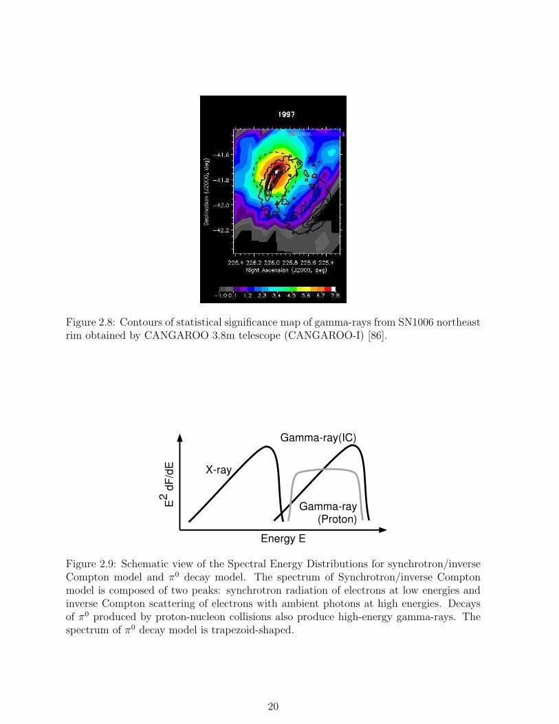
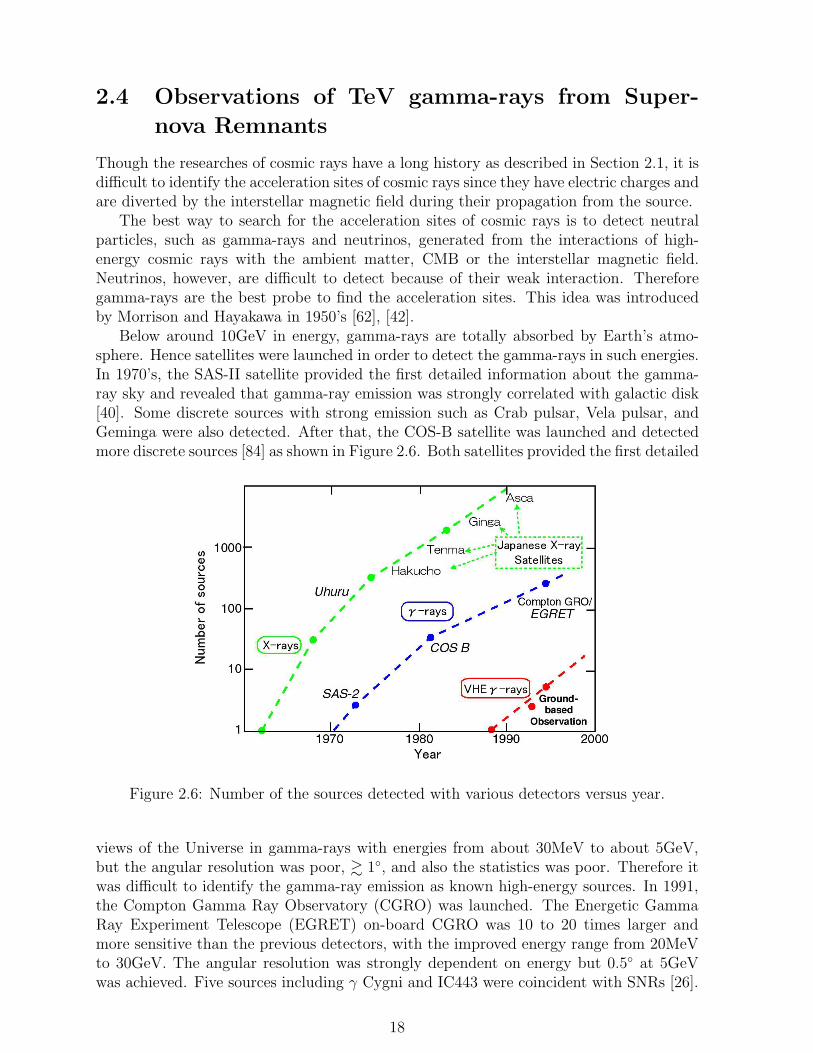
Figure 2.8: Contours of statistical significance map of gamma-rays from SN1006 northeastrim obtained by CANGAROO 3.8m telescope (CANGAROO-I) [86].

Figure 2.9: Schematic view of the Spectral Energy Distributions for synchrotron/inverseCompton model and π0 decay model. The spectrum of Synchrotron/inverse Comptonmodel is composed of two peaks: synchrotron radiation of electrons at low energies andinverse Compton scattering of electrons with ambient photons at high energies. Decaysof π0 produced by proton-nucleon collisions also produce high-energy gamma-rays. Thespectrum of π0 decay model is trapezoid-shaped.

20

10-2

10-1

100

101

102

νSν or ε2 dF/dε

[ eV cm-2 s-1 ]

1015

1010

105

100

10-5

photon energy ε [eV]

Synchrotron

InverseComptonB = 4 µG

radio

IRASupper limit

ROSAT

ASCA

EGRETupper limit

CANGAROO

π0 decayparent protonspectrum

α=2.2Emax=5e15no*E50=2.5

Figure 2.10: Spectral Energy Distribution observed from the NE rim of SN1006 [85],where observed fluxes or upper limits of radio [78], infrared, soft X-ray (estimated fromWillingale et al. [93]), hard X-ray [72], GeV gamma-rays (calculated from the EGRETarchival data), and TeV gamma-rays are presented. Solid lines are the fits based on themodel of synchrotron/inverse Compton model and π0 decay.

21

tection of TeV gamma-rays from SN1006 could not be the clear evidence of the protonacceleration. Meanwhile several SNRs were found by the ROSAT all-sky survey. The ob-servations of ASCA revealed intense non-thermal emission from RX J1713.7−3946 [56],RCW86 [8], and RX J0852.0−4622 [82] [88]. These SNRs are on the galactic plane.Molecular clouds surrounding them can be a target of accelerated proton interactions.Detections of gamma-rays in sub-TeV energies from these SNRs could be the evidencesof proton acceleration. The northwest (NW) rim of of RX J1713.7−3946 was observed byCANGAROO telescope [63] [25]. Figure 2.11 shows the contour map of statistical signifi-cance map of RX J1713.7−3946 northeast rim obtained by CANGAROO 10-m telescope[25]. Figure 2.12 shows the SED from RX J1713.7−3946 [25]. The spectrum was a good

Figure 2.11: Contours of statistical significance map of RX J1713.7−3946 northeast rimobtained by CANGAROO 10m telescope [25].

match to that from π0 decay and could not be explained by other mechanisms. Thereforethis detection of TeV gamma-rays was thought to be the direct evidence of the protonacceleration. This conclusion, however, was objected by Butt et al. [15] from the pointof the density of molecular cloud. Recently the NANTEN observation revealed that amolecular cloud of ∼200 solar masses was clearly associated with the TeV gamma-raypeak [29] which denied the objection by Butt el al. Reimer and Pohl [77] also claimed thespectrum of the nearest EGRET source was inconsistent with the predicted spectrum byπ0 decay especially in GeV region. The recent non-linear acceleration theory predictedand suggested that the cosmic ray power-law index can be less than 2 and may solvethe above problem [11]. Simple synchrotron/inverse Compton model must be consideredagain if the emission regions in X-ray and TeV energies are different. When the accel-eration and emission regions are different, especially in size, TeV flux could be differentfrom that predicted by the simple synchrotron/inverse Compton model (two-zone model[1]). In order to explain the TeV emission of RX J1713.7−3946 with this scheme, thevolume ratio of VTeV /VX = 1000 is necessary [73]. There is, however, no other physicalevidence for this value. The HEGRA group detected TeV gamma-rays from CassiopeiaA using a stereoscopic Cherenkov telescope system [3]. From the hard X-ray continuum,a lower limit to the average magnetic field was estimated to be 0.5 mG [89]. Thereforethe TeV spectrum is difficult to explain by inverse Compton scattering of electrons due tosuch a high magnetic field. By this discussion Cassiopeia A is thought to be the protonacceleration site. However the evidences for proton acceleration are still sparse and are

22

10-1

100

101

102

E2 d

F/dE

or E

F(>

E)

(eV

cm

-2 s

-1)

101010510010-5

Photon energy, E (eV)

radio

ASCA CANGAROO

EGRET

Figure 2.12: Spectral Energy Distribution from RX J1713.7−3946, and emission models[25]. The radio data was obtained by ATCA [21]. The shaded area between thick linesshows the ASCA GIS data. The EGRET upper limit corresponds to the flux of 3EGJ1714−3857 [41]. The TeV gamma-ray points show CANGAROO data. Lines showmodel calculations: synchrotron emission (solid line), inverse Compton emission (dottedlines). bremsstrahlung (dashed lines) and emission from π0 decay. Inverse Comptonscattering and bremsstrahlung are plotted for two cases: 3µG (upper curves) and 10µG(lower curves).

23

not conclusive.In order to establish the hypothesis that the Galactic cosmic rays are mainly accel-

erated by the SNRs, much more evidences are needed. Other SNRs with non-thermalX-ray emission should be observed with IACTs, such as RCW86 and RX J0852.0−4622,which have been already observed by CANGAROO. The data analysis and results of RXJ0852.0−4622 were reported in this thesis. The details of RX J0852.0−4622 observationswere described in the next section. Further studies will be also carried out by the nextgeneration Cherenkov telescopes with lower energy threshold such as CANGAROO-III.

2.5 SNR RX J0852.0−4622 (G266.2−1.2)

RX J0852.0−4622 (G266.2−1.2) is a SNR located at the southeast corner of the Vela SNR.It was discovered at X-ray energies during the ROSAT all-sky survey by Aschenbach [5]shown in Figure 2.13. Its apparent size was around 2. The 1.156-MeV 44Ti line was

Figure 2.13: Soft X-ray images of Vela SNR observed by ROSAT. This is for photonenergies < 1.3 keV. RX J0852.0−4622 is on the lower left.

detected with COMPTEL by Iyudin et al. [49]. 44Ti decays into 44Sc emitting two hardX-ray lines of 68 keV and 78keV. The lifetime of 44Ti is 60yr [67] [36]. From these values,the weighted mean of the lifetime was derived to be 90.4±1.3 years [49]. The effective44Ti lifetime could be larger, depending on the degree of ionization of the 44Ti and itsLorentz factor. 44Sc decays further to 44Ca while emitting a gamma-ray line at 1.156MeVwith the lifetime of 3.9 hr. By combining the gamma-ray line flux and the X-ray diameterwith an assumed typical 44Ti yield, and taking as representative an expansion velocityof ∼ 5000km s−1 for the supernova ejecta, the distance and age were estimated to be∼200 pc and ∼680yr, respectively [49]. It was not recorded historically. This may havebeen seen in measurements of nitrate abundances in Antarctic ice cores [14]. Supernovae

24

can produce NO−3 when their radiations ionize the molecules in the atmosphere. The X-

ray emission line at 4.1±0.2 keV was only detected in the northwest shell by ASCA [88].This line was thought to come from highly ionized Ca. We, however, cannot distinguishamong the Ca isotopes using X-ray data. Assuming that most of the Ca is 44Ca, the ageof RX J0852.0−4622 was estimated to be around 1000 yr combining the amount of 44Caand the observed flux of the 44Ti [88]. Aschenbach, Iyudin, and Schonfelder estimated thedistance and age again [6]. They estimated the expansion velocity using X-ray spectraat the limb obtained by ROSAT. The minimal, best-estimate, and maximal expansionvelocities were 2000, 5000, and 10000 km s−1, respectively. Model calculations providea range for the mass yield of 44Ti. Considering these uncertainties, the upper limit ofthe distance of RX J0852.0−4622 was estimated to be 500pc and 1100yrs for the age.Chen and Gehrels have also used the X-ray temperature obtained from ROSAT datafor the central region to derive a range of 2000-5000 km s−1 [17]. If this is true, theremnant is currently expanding too slowly to be caused by a Type Ia supernova. Theestimation of Aschenbach, Iyudin, and Schonfelder, however, allow it to be a Type Iafor the expansion speed. The central region of the SNR was observed with ROSAT [5],ASCA [82], BeppoSAX [59], and Chandra [74]. Based on the X-ray-to-optical flux ratio,the X-ray source in the central region was likely the compact remnant of the supernovaexplosion that created the RX J0852.0-4622. Figure 2.14 shows the hard X-ray imagesof RX J0852.0−4622 observed by ASCA GIS [82] [88]. The images clearly shows shell-

Figure 2.14: Hard X-ray image of RX J0852.0−4622 observed by ASCA GIS (E =0.7-10 keV) [82]. The image consists of a mosaic of seven individual fields. Contours representthe outline of the Vela SNR as seen in ROSAT survey data with the PSPC.

like morphology. The hard X-ray spectrum was well fitted by a power law. The matterdensity of the X-ray peak was estimated to 2.9×10−2d

−1/21 f−1/2 [H/cm−3], where d and f

are the distance normalized to 1kpc and the filling factor, respectively [82]. While simple

25

scaling of the column density to estimate the distance was clearly rather uncertain, itappears that the remnant is at least several times more distant than Vela. The distanceto the Vela SNR was estimated to be 250±30 pc using Ca II and Na I absorption linespectra toward the OB stars in the direction of Vela SNR [16]. The distances to the OBstars were well determined using trigonometric parallaxes and spectroscopic parallaxesbased on photometric colors and spectral types. The radio emission was found with theParkes radio-telescope [18] [20]. The fluxes at 2.42 and 1.40 GHz were 33±6Jy and 40±10Jy, respectively [20]. The spectral index were −0.40±0.15 at the northern section of theshell [20] Figure 2.15 shows the 4.85 GHz radio images [20]. Shell-like morphology can

Figure 2.15: Radio images at 4.85GHz observed by the Parkes radio-telescope, centered onRX J0852.0−4622 2.15. The angular resolution is' 5′ , and the rms noise is approximately8 mJy beam−1. The grey-scale wedge is labelled in units of Jy beam−1. The black circleis centered on the X-ray coordinates of the source and is 1.8 in angular diameter.

be seen. But the confusing structures from Vela SNR exist. CO observations showed therichness of large molecular clouds around RX J0852.0−4622 in the Vela Molecular Ridge[58]. They can be targets of proton-nucleon collisions. The detailed morphology wasmapped with the NANTEN 4m milli-metre radio telescope [61]. Figure 2.16 shows theCO map around the Vela SNR. CO observations has a better accuracy to determine thedistance than 21cm radio observations because of their narrow Doppler broadening. Thecorrelation between RX J0852.0-4622 and the molecular clouds were not yet investigated.From above observations, the characteristics of RX J0852.0−4622 are similar to thoseof RX J1713.2−3946. 100-TeV electrons can be expected from the non-thermal X-rayemission. If the ambient magnetic field is not so strong, TeV gamma-rays from inverseCompton scattering are produced. On the other hand, TeV gamma-rays from π0 decayproduced by proton-nucleon collisions may be detected because the nearby molecularclouds exists.

26

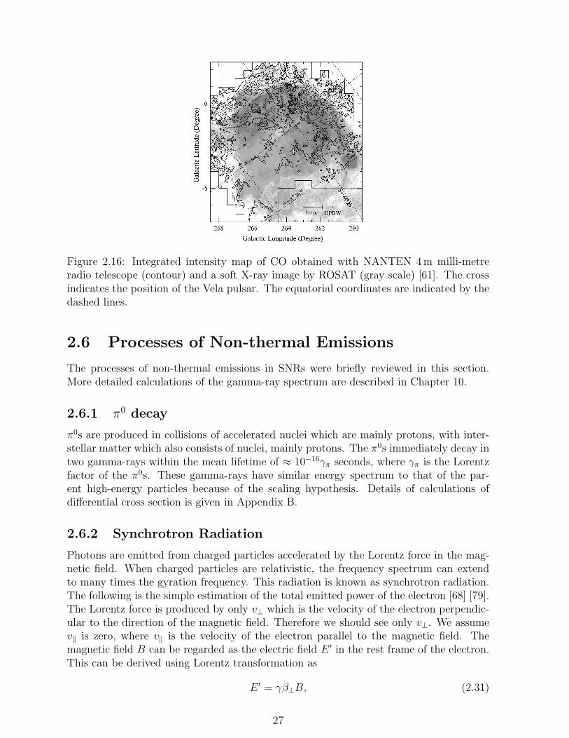
Figure 2.16: Integrated intensity map of CO obtained with NANTEN 4m milli-metreradio telescope (contour) and a soft X-ray image by ROSAT (gray scale) [61]. The crossindicates the position of the Vela pulsar. The equatorial coordinates are indicated by thedashed lines.

2.6 Processes of Non-thermal Emissions

The processes of non-thermal emissions in SNRs were briefly reviewed in this section.More detailed calculations of the gamma-ray spectrum are described in Chapter 10.

2.6.1 π0 decay

π0s are produced in collisions of accelerated nuclei which are mainly protons, with inter-stellar matter which also consists of nuclei, mainly protons. The π0s immediately decay intwo gamma-rays within the mean lifetime of ≈ 10−16γπ seconds, where γπ is the Lorentzfactor of the π0s. These gamma-rays have similar energy spectrum to that of the par-ent high-energy particles because of the scaling hypothesis. Details of calculations ofdifferential cross section is given in Appendix B.

2.6.2 Synchrotron Radiation

Photons are emitted from charged particles accelerated by the Lorentz force in the mag-netic field. When charged particles are relativistic, the frequency spectrum can extendto many times the gyration frequency. This radiation is known as synchrotron radiation.The following is the simple estimation of the total emitted power of the electron [68] [79].The Lorentz force is produced by only v⊥ which is the velocity of the electron perpendic-ular to the direction of the magnetic field. Therefore we should see only v⊥. We assumev‖ is zero, where v‖ is the velocity of the electron parallel to the magnetic field. Themagnetic field B can be regarded as the electric field E ′ in the rest frame of the electron.This can be derived using Lorentz transformation as

E ′ = γβ⊥B, (2.31)

27

where γ and β⊥ are the Lorentz factor of the electron and v⊥/c (c is light speed), respec-tively. Using the Larmor’s formula, the total emitted power in the rest frame is givenas

P ′ =2e2

3c3

(eγβ⊥B

m

)2

= 2σTcγ2β2⊥

B2

8π, (2.32)

where e and m are the charge of the electron and the rest mass of the electron, respectively.For an isotropic distribution of velocities it it necessary to average this formula over allangles for an given speed β. Let α be the pitch angle, which is the angle between themagnetic field and the velocity. Then we obtain

〈β2⊥〉 =

∫β2⊥ sin α2dΩ

4π=

2β2

3, (2.33)

where Ω is the solid angle, respectively. And the result is

P ′ =4

3σTcγ2β2UB, (2.34)

where σT and UB are the cross section of Thomson scattering and the energy density ofthe magnetic field, respectively. The total emitted power P ′ is the Lorentz invariance andis preserved under Lorentz transformation. Hence P is give as

P =4

3σTcγ2β2UB. (2.35)

Synchrotron radiation is important only for electrons since P is proportional to 1/m2 forhigh-energy particles from Equation (2.35). The frequency spectrum can extend to manytimes the gyration frequency. Figure 2.17 shows the spectral distribution of the power ofthe total (over the directions) radiation from charged particles moving in a magnetic fieldas a function of ν/νC [35], where ν and νC are the frequency of the emitted photons andνC = 3eBγ2/4πmc. The spectrum has a roughly monochromatic peak.

2.6.3 Inverse Compton Scattering

When relativistic electrons move in the photon field , the scattered photons by Comptonscattering gains its energy from the electron. This process is called inverse Compton (IC)scattering. The energy of the ambient photon in the rest frame of the electron is given as

hν∗ = γhν(1 + β cos θ), (2.36)

where h, ν∗, γ, ν, β, and θ are Planck constant, the frequency of the photon in thelaboratory frame, the Lorentz factor of the electron, the frequency of the electron in therest frame of the electron, the velocity of the electron, and the angle of incidence fromthe direction of the electron motion in the laboratory frame, respectively. Assuming thedistribution of the ambient photons is isotropic, the photon energy is γhν. In case ofγhν ¿ mc2, where m is the rest mass of the electron, the scattering in the rest frame of

28

Figure 2.17: Spectral distribution of the power of the total (over the directions) radiationfrom synchrotron radiation [35]. ν and νC are the frequency of the emitted photons andνC = 3eBγ2/4πmc.

the electron is approximately Thomson scattering, i.e. elastic. Hence the energy of thescattered photon is given as

hν ′ = γhν∗(1 + cos ϕ) ≈ γ2hν, (2.37)

where ν ′ and ϕ are the frequency of the scattered photon in the laboratory frame and thescattering angle of the photon in the rest frame, respectively. The energy of the scatteredphoton exactly averaging over angles is given as

h′ν =4

3γ2hν. (2.38)

Using Equation (2.38), the energy loss rate of the electron is given as

−dE

dt=

4

3σTcγ2U, (2.39)

where σT, and U are the cross section of Thomson scattering and the energy density ofthe radiation field nhν (n is the number density of ambient photons), respectively.

2.6.4 Bremsstrahlung

When charged particles are passed through the Coulomb field of a nucleus, photons areemitted. This is called bremsstrahlung. As described in Subsection 3.2.1 in detail, thecross section and the emitted power of bremsstrahlung are proportional to 1/m2, wherem is the rest mass of the charged particle. Therefore bremsstrahlung is important forelectrons and is negligible for nuclei.

29

Chapter 3

Imaging Air Cherenkov Technique

3.1 Overview

As was discussed in the previous chapter, the detection of TeV gamma-rays is a goodway to study particle accelerations. However, it is not easy to detect significant signalsin TeV energies due to the small statistics at such energies. Besides the depth to stop allparticles produced in the cascade above TeV energies is too large for the satellite. HenceTeV gamma-rays penetrate into the atmosphere without being detected in the space.The earth, however, has sufficient material, i.e. the atmosphere itself. Therefore verylarge-scale detector can be made using the atmosphere as a part of detector. When thegamma-rays and cosmic rays penetrate into the atmosphere, they interact with moleculesof air and generate electromagnetic and/or hadronic cascade, respectively. This phe-nomenon is well known as Extensive Air Showers (EASs). EASs develop and the numberof the particles in EASs reaches the maximum (shower max) approximately at an orderof 10km from the sea level. It is impossible to detect such huge EASs by calorimetricways like satellites because of low flux. Instead of this method, the optical lights fromthe showers, such as fluorescence and/or Cherenkov radiation can be used as informationof showers. Fluorescence is isotropic radiation. Hence it is difficult to detect it on theground due to its weakness for TeV gamma-rays. On the other hand, Cherenkov radia-tion becomes strongly peaked in the direction of particle motion, i.e. roughly along theaxis of EASs. It spreads on the ground with an order of 100m. If the detectors havethe large area collecting photons such as 10m2, it is possible to detect such a light as ashort-time pulse of ∼10nsec. Furthermore, the extremely larger effective area (3×104m2)than the satellite can overcome small statistics. It, however, is still difficult to detect TeVgamma-rays without removing showers which are generated from cosmic rays. Fortunatelydevelopments detecting profiles of showers can distinguish gamma-rays from cosmic rays.Imaging air Cherenkov technique can detect the difference in the images of the photonson the ground and distinguish them. CANGAROO telescope is one of the imaging airCherenkov telescope (IACT) for realizing such a technique. The details of the EASs,Cherenkov radiation, and imaging air Cherenkov technique are described in the followingsections.

30

3.2 Extensive Air Showers

When gamma-rays and cosmic rays in TeV energies penetrate into the atmosphere, theyinteract with the atmosphere. Showers are classified by the primary particles, i.e electro-magnetic particles (electrons, positrons, and gamma-rays) and hadrons (mainly protonsand nuclei) .

3.2.1 Electromagnetic Showers

When the energetic electrons pass through the matter, they emit photons due to theiracceleration in the Coulomb field of the atomic charge of the nuclei (bremsstrahlung).Each of the secondary photons then reproduces electron-positron pairs through the paircreation process. As a result of these interactions, the number of both electrons andphotons increases. This phenomenon is called electromagnetic shower. The probabilityof the photon emission and that of pair creation were calculated by Bethe and Heitler[45]. The probability for emission of a photon in the energy interval (E ′, E ′ + dE ′) by anelectron of energy E after traversing a medium of thickness dx g/cm2 is given as

ΦdE ′

E= 4

137· N

A· z2r2

0dE′E· E

E′

[1 +

(1− E′

E

)2 − 23

(1− E′

E

)log (191Z− 1

3 ) + 19

(1− E′

E

)]

= 4137· N

A· z2r2

0dvv

[1 + (1− v)2 − 2

3(1− v)

log (191Z− 1

3 ) + 19(1− v)

], (3.1)

where Z and A are the atomic number, and atomic weight of the traversed matter,respectively, N is Avogadro’s number, r0 is the classical electron radius e2/mc2, and v ≡E ′/E. Figure 3.1 shows the spectrum of bremsstrahlung approximately calculated fromEquation (3.1). From Equation (3.1), the energy loss of bremsstrahlung is approximated

0

20

40

60

80

100

120

140

0 0.2 0.4 0.6 0.8 1

Arb

itrar

y un

it

v=E’/E

f(x)

Figure 3.1: Spectrum of bremsstrahlung approximately calculated from Equation (3.1),where E, E’, and v are the electron energy, emitted photon energy, and E’/E, respectively.The probability is ≈ 1/v at v ¿ 1.

as

−dE

dx=

∫ E

0

E ′ · ΦdE ′

E≈ X−1E, (3.2)

where we put

X−1 =4

137

N

Az2r2

0 log Z− 13 . (3.3)

31

X is called “radiation length”, which is ∼ 37 g/cm2 in the air. The probability of paircreation by a photon of energy E generating an electron in (E ′, E ′+dE ′) is again approx-imated as

ΨdE ′

E= 4

137· N

A· z2r2

0dE′E

[(E′E

)2+

(1− E′

E

)2+ 2

3E′E

(1− E′

E

)log (191Z− 1

3 )− 19

E′E

(1− E′

E

)]

= 4137· N

A· z2r2

0dv[

(v)2 + (1− v)2 + 23v (1− v)

log (191Z− 1

3 )− 19v (1− v)

]. (3.4)

Figure 3.2 shows the spectrum of pair creations approximately calculated from Equation(3.4). Using Equation (3.4), the total probability of pair creation is given as

0.65

0.7

0.75

0.8

0.85

0.9

0.95

1

0 0.2 0.4 0.6 0.8 1

Arb

itrar

y un

it

v=E’/E

f(x)

Figure 3.2: Spectrum of pair creations approximately calculated from Equation (3.4),where E, E ′, and v are the photon energy, created electron energy, and E ′/E, respectively.

∫ E

0

ΨdE ′

E≈ 7

9X−1. (3.5)

Except for the above two processes, the ionization loss and the multiple Coulomb scat-tering effect must be considered. Ionization loss can be neglected if the electron has aenergy of more than the critical energy (≈ 700/Z MeV; Z is the atomic number). In caseof the air, the critical energy is ∼ 81 MeV. Assuming the ionization loss and multipleCoulomb scatterings are neglected, the pair creation and the Bremsstrahlung occur onceper radiation length. When the electron energy becomes near the critical energy, the ion-ization loss becomes dominant and the shower development stops. In order to estimatethe shower development, we adopt a simple model where the energy dissipation of theparticles occurs only through the constant ionization loss. The equation is given as

ε

∫ T

0

2tdt = E0, (3.6)

where T , ε and E0 are the depth at the shower maximum, the ionization loss per radiationlength, and the energy of primary particle, respectively. Here we assume that the numberof particles in showers is 2t at depth t. From Equation (3.6), T and E0 are given as

T ∝ ln

(E0

ε

), (3.7)

Nmax ' 2T ∝ E0, (3.8)

32

where Nmax is the number of particles in the shower maximum. More practical forms aregiven as

T ≈ ln

(E0

81MeV

)+

1

2, (3.9)

Nmax ≈ 1000

(E0

1TeV

). (3.10)

T and Nmax are ∼10 and 1000 at 1TeV, respectively. At these processes in the showers,the transverse momenta of the secondary particles are considered to be an order of mec/2(i.e. relativistic beaming). For example, the Lorentz factor of the electron with the criticalenergy is ∼ 160 and the emission angle is ∼ 1/γ ≈ 0.006 radian ≈ 0.35.

As was described above, particle interactions in the matter are characterized by X(g/cm2), which is the depth from the top of the atmosphere. Figure 3.3 shows the defini-tions of the variables representing the height and depth of the atmosphere. XV is defined

h=0 On the ground

Top ofthe atmosphere

X=0

X

hh

XV

V

S

S

Shower max(X ~10)V

Figure 3.3: Definitions of the variables representing the height and depth of the atmo-sphere. X is the depth from the top of the atmosphere (g/cm2). h is the distance fromthe see level (cm). The shower max of gamma-rays at around 1 TeV is XV ∼ 10.

as

XV (hV ) =

∫ ∞

hV

ρ(h′)dh′, (3.11)

where ρ(h) is the density of the atmosphere at the height of h. Assuming the atmosphere isthe ideal gas and using the pressure p(hV ) = XV (hV ) and the density ρ(hV ) = −dXV /dhV ,the equation of state is written as

p

ρ=

XV

−dXV /dhV

= RT, (3.12)

where R is Rydberg constant. From Equation (3.12), the depth XV is given as

XV = X0 exp (−hV /h0), (3.13)

33

where X0 ' 1030g/cm2, and h0 = RT is the scale height. The depth of the atmosphere isroughly parameterized by Equation (3.13) and the scale height h0(T ). For example, XV sare 1X, 7X and 10X at 23km, 10km and 8km from the sea level, respectively.

Figure 3.4 shows a schematic view of electromagnetic showers of 1TeV gamma-raysin the air. In summary, gamma-rays in 1TeV energies penetrate into the air. First

Ele

vatio

n (k

m)

20

10

0

Dep

th 1X

7X10X n=1.0001

n=1.000328XD

epth 1X

2X

3X

e + e -

photon

50m

Figure 3.4: Schematic view of electromagnetic showers of 1TeV gamma-rays in the air.X and n are the radiation length of the electron in the air and the refractive index.

interaction occurs at a point of 20km from the see level, corresponding to one radiationlength. The showers do not develop quickly because of the low pressure there. The showersize suddenly increases exponentially around altitude of ∼ 10 km. Their whole shapesare thin. After the shower maximum, particles lose their energy due to the ionization lossand stop shower development.

3.2.2 Hadronic Showers

The mean free path of nucleons in air in TeV energies is ≈ 100g/cm2 (inelastic collisionlength). The first inelastic collision occurs at a height of ≈ 16 km according to the U.S.Standard Atmosphere table. The first proton-proton collision produces pions and sec-ondary nucleons. Figure 3.5 shows a schematic interaction processes of hadronic showers[92]. Typical transverse momentum of the secondary particle is 300 ∼ 400 MeV, whichis an order of magnitude larger than the case of electromagnetic showers. Therefore the

34

Figure 3.5: Schematic interaction processes of hadronic showers [92].

35

opening angle of the shower development is larger than that of the electromagnetic show-ers. Experimentally shower max is known to be located around 3-inelastic interactionlength, i.e., 10 km altitude ≈ 300 g/cm2. The secondary π0s have very short life times,≈ 10−16 sec, before decaying to two gamma-rays. The secondary nucleons and chargedpions proceed to the next collisions with nucleons in the air, which produce pions andsecondary nucleons again until their energies drop below those required for multiple pionproduction, i.e. about 1GeV. Below 1GeV, the secondary protons around 1GeV lose theirenergy due to the ionization loss and its decay. The charged pions decay to muons andmuon neutrinos via

π+ → µ+ + νµ,

π− → µ− + νµ. (3.14)

The life times of charged pions are ≈ 10−8 sec. The low energy muons decay after ∼ 2µsecto positrons, electrons and muon neutrinos via

µ+ → e+ + νe + νµ,

µ− → e− + νe + νµ. (3.15)

The produced positrons and electrons form the electromagnetic showers. The high-energymuons (≥2GeV) reach the Earth’s surface because its interaction is weak. The hadronicshowers have the extended structure because of the above mentioned reasons, comparedto the electromagnetic showers. Figure 3.6 shows the showers of gamma-rays and cosmicrays in 1TeV simulated by the Monte Carlo methods.

Figure 3.6: Showers of gamma-rays (left) and protons (right) in 1TeV simulated by theMonte Carlo methods.

36

3.3 Cherenkov Radiation

Blackett in 1948 predicted that the Cherenkov light from EASs should be detectablefrom the surface on the earth. It was confirmed observationally several years later byGalbraith and Jelley [32]. We introduce the characteristics of the Cherenkov radiation inthis section. Suppose an electron is moving faster than the light in the medium which isa perfect isotropic dielectric material. Figure 3.7 shows a schematic view of Cherenkovradiation. Using Huygens’s principle, the wave front is determined as shown in the Figure

v t

c’ t

c’=c/n

+-+

-+-

+-+

-+-

E=0E

e-C

Figure 3.7: Schematic view of Cherenkov radiation, where n, c, c′, v, ∆t and E are therefractive index, the light speed in the vacuum, the light speed in the dielectric medium,the velocity of the electron, a time and electric field, respectively.

3.7 and cos θC is given as

cos θC =1

βn, (3.16)

where v, β and n are the velocity of the electron, v/c and the refractive index, respectively.At the back of the wave front, the medium is polarized by the electric field. The atoms inthe medium behave like dipoles. Each dipole radiates a short electromagnetic pulse. FromEquation (3.16), θC of the electrons of the critical energy in the air is ≈ 0.7 degree at 10kmfrom the sea level, where n is ≈ 1.0001. On the ground, the distributions of the abovephotons are the circle with the radius of 10km × tan (0.7) ≈ 120m. This characteristicmakes the effective area extremely large (3×104m2). Figure 3.8 shows the examples ofthe images and the lateral distributions of photons produced from gamma-ray showersin 1TeV. Figure 3.9 shows the examples of protons in 3TeV. Frank and Tamm estimatedthe light yield of Cherenkov radiation by the classical theory [28]. The radiation energyby an electron of angular frequency ω after traversing a medium of thickness dl g/cm2, is

37

Figure 3.8: Images (left) and the lateral distributions (right) of photons produced fromgamma-ray showers in 1TeV.

Figure 3.9: Images (left) and the lateral distributions (right) of photons produced fromproton showers in 3TeV.

38

given asdW

dl=

e2

c2

∫

βn>1

(1− 1

β2n2)ωdω, (3.17)

where e is the electron charge. Cherenkov radiation is independent of ω in terms ofthe number of photons because it does not have any specific frequency. Therefore thenumber of photons emitted from Cherenkov radiation is proportional to dλ/λ2, where λis the wavelength of the emitted photons. The number of photons emitted by an electronbetween wavelengths λ1 and λ2 is given from Equation (3.17) as

N = 2παl(1

λ1

− 1

λ2

)(1− 1

β2n2), (3.18)

where α and n are the fine structure constant = e2/~c = 1/137 and the average refractiveindex of the medium. From Equation (3.18), the number of photons emitted from therelativistic electron in the air per meter is ∼ 10 at the wavelengths between 300nm and600nm corresponding to the range typically covered by the photomultiplier tubes (PMTs).The atmosphere, however, scatters and absorbs these photons. Figure 3.10 shows thetransmission of air. Including all effects, the photon spectrum peaks at around 300nm.

Figure 3.10: Transmission of the Cherenkov photons.

The detectors of IACTs must cover such a energy range.

3.4 Imaging Air Cherenkov Technique

Most of the showers are generated from cosmic rays. In order to distinguish betweenhadronic showers and electromagnetic showers, the characteristics of directional distribu-

39

tions of photons at the ground provides useful information. The photon distributions aredifferent due to the shower developments as were described in the Section 3.2. Figure3.11 shows examples of the distributions of photons on the focal plane of IACTs. Hillas

Figure 3.11: Examples of the distributions of photons on the camera plane of IACTs.

introduced the parameters which characterizes the shapes of the photon images (Hillasparameters) [46]. The most important parameter α (image orientation angle) was intro-duced by Punch et al [75]. Figure 3.12 shows a schematic view of Hillas parameters andα. The root mean square (RMSs) spreads of light along the major axis and the minor

Alpha

Length

Width

SourceDistance

Centroid

Figure 3.12: Hillas parameters [46] and α [75].

axis are Length and Width, respectively. Distance is the distance between the centroid ofthe image and the source position. α is the angle between the major axis and the linewhich connects the source position to the centroid of the image. Asymmetry is the cubicroot of the third moment of the image along the major axis. The details are described inAppendix A.

As shown in Figure 3.11, the gamma-ray images are compact compared with protonimages. Therefore the selection of the compact images using Length and Width is effective.

40

The most effective way, however, is the so-called α cut. The gamma-ray images shouldbe concentrated near α = 0 because the shower axis is parallel to the pointing directionof the telescope. On the other hand, the axes of the showers generated from cosmic rayspoint to various directions and the images are not concentrated to the specific value of α.Figure 3.13 shows the schematic view of images generated from gamma-rays and protons.Whipple group first detected Crab nebula using above parameters [76] and verified the

Figure 3.13: Schematic view of images generated from gamma-rays and protons.

capability of IACTs. Figure 3.14 shows the example of the α distributions obtained bythe Whipple Observatory [48]. The CANGAROO-II telescope has a 10-m reflector aslarge as the Whipple telescope described in the next chapter. Most important differencebetween these two is that Whipple is located in the northern hemisphere and we are inthe southern hemisphere.

41

Figure 3.14: Distributions of α about Markarian 421 obtained by the Whipple Observatory[53]. The solid line and the dotted line show the ON-source data and the OFF-sourcedata, respectively.

42

Chapter 4

The CANGAROO-II 10-m Telescope

The CANGAROO (Collaboration of Australia and Nippon (Japan) for a GAmma RayObservatory in the Outback) 1 is the international collaborated experiment for very high-energy gamma-ray observations using IACTs since 1992. The observation site is locatednear Woomera, South Australia (136 46′E, 31 06′ S, 220 m a.s.l.).

The CANGAROO-II project is exploring the southern sky at gamma-ray energies of0.4 ∼ 100 TeV. Figure 4.1 is a picture of the CANGAROO-II 10-m telescope. Beforeproceeding to this project, we used CANGAROO-I telescope with the 3.8m diameterreflector [39] and detected TeV gamma-ray emission such objects as pulsar nebulae (PSR1706−44 [54], the Crab [87]), and SNRs (SN1006 [86], RX J1713.2−3946 [64]). TheCANGAROO-II 10-m telescope had been in operation since April, 2000, and detectedSNR RX J1713.2−3946 [25] and the active galactic nuclei Mrk 421 [71], and the starburst

1The collaborators of CANGAROO group:A. Asahara1, G.V. Bicknell2, R.W. Clay3, Y. Doi4, P.G. Edwards5, R. Enomoto6, S. Gunji4, S. Hara6,T. Hara7, T. Hattori8, Sei. Hayashi9, C. Itoh10, S. Kabuki6, F. Kajino9, H. Katagiri6, A. Kawachi6, T.Kifune11, L.T. Ksenofontov6, H. Kubo1, T. Kurihara8, R. Kurosaka6, J. Kushida8 Y. Matsubara12, Y.Miyashita8, Y. Mizumoto13 M. Mori6, H. Moro8, H. Muraishi14 Y. Muraki12 T. Naito7 T. Nakase8, D.Nishida1, K. Nishijima8, M. Ohishi6, K. Okumura6, J.R. Patterson3, R.J. Protheroe3, N. Sakamoto4, K.Sakurazawa15, D.L. Swaby3, T. Tanimori1, H. Tanimura1, G. Thornton3, F. Tokanai4, K. Tsuchiya6, T.Uchida6, S. Watanabe1, T. Yamaoka9, S. Yanagita16, T. Yoshida16, T. Yoshikoshi17

(1) Department of Physics, Graduate School of Science, Kyoto University, Sakyo-ku, Kyoto 606-8502,Japan(2) Research School of Astronomy and Astrophysics, Australian National University, ACT 2611, Australia(3) Department of Physics and Mathematical Physics, University of Adelaide, SA 5005, Australia(4) Department of Physics, Yamagata University, Yamagata, Yamagata 990-8560, Japan(5) Institute of Space and Astronautical Science, Sagamihara, Kanagawa 229-8510, Japan(6) Institute for Cosmic Ray Research, University of Tokyo, Kashiwa, Chiba 277-8582, Japan(7) Faculty of Management Information, Yamanashi Gakuin University, Kofu, Yamanashi 400-8575,Japan(8) Department of Physics, Tokai University, Hiratsuka, Kanagawa 259-1292, Japan(9) Department of Physics, Konan University, Kobe, Hyogo 658-8501, Japan(10) Ibaraki Prefectural University of Health Sciences, Ami, Ibaraki 300-0394, Japan(11) Faculty of Engineering, Shinshu University, Nagano, Nagano 480-8553, Japan(12) Solar-Terrestrial Environment Laboratory, Nagoya University, Nagoya, Aichi 464-8602, Japan(13) National Astronomical Observatory of Japan, Mitaka, Tokyo 181-8588, Japan(14) School of Allied Health Sciences, Kitasato University, Sagamihara, Kanagawa 228-8555, Japan(15) Department of Physics, Tokyo Institute of Technology, Meguro, Tokyo 152-8551, Japan(16) Faculty of Science, Ibaraki University, Mito, Ibaraki 310-8512, Japan(17) Department of Physics, Osaka City University, Osaka, Osaka 558-8585, Japan

43

Figure 4.1: CANGAROO-II 10-m telescope.

44

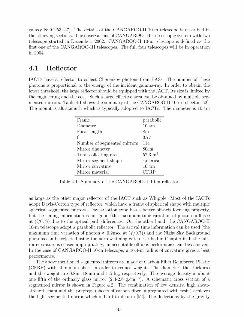
galaxy NGC253 [47]. The details of the CANGAROO-II 10-m telescope is described inthe following sections. The observations of CANGAROO-III stereoscopic system with twotelescope started in December, 2002. CANGAROO-II 10-m telescope is defined as thefirst one of the CANGAROO-III telescopes. The full four telescopes will be in operationin 2004.

4.1 Reflector

IACTs have a reflector to collect Cherenkov photons from EASs. The number of thesephotons is proportional to the energy of the incident gamma-ray. In order to obtain thelower threshold, the large reflector should be equipped with the IACT. Its size is limited bythe engineering and the cost. Such a large effective area can be obtained by multiple seg-mented mirrors. Table 4.1 shows the summary of the CANGAROO-II 10-m reflector [52].The mount is alt-azimuth which is typically adopted to IACTs. The diameter is 10.4m

Frame parabolicDiameter 10.4mFocal length 8mf 0.77Number of segmented mirrors 114Mirror diameter 80cmTotal collecting area 57.3 m2

Mirror segment shape sphericalMirror curvature 16.4mMirror material CFRP

Table 4.1: Summary of the CANGAROO-II 10-m reflector.

as large as the other major reflector of the IACT such as Whipple. Most of the IACTsadopt Davis-Cotton type of reflector, which have a frame of spherical shape with multiplespherical segmented mirrors. Davis-Cotton type has a better off-axis focusing property,but the timing information is not good (the maximum time variation of photon ≈ 6nsecat (f/0.7)) due to the optical path differences. On the other hand, the CANGAROO-II10-m telescope adopt a parabolic reflector. The arrival time information can be used (themaximum time variation of photon ≈ 0.2nsec at (f/0.7)) and the Night Sky Backgroundphotons can be rejected using the narrow timing gate described in Chapter 6. If the mir-ror curvature is chosen appropriately, an acceptable off-axis performance can be achieved.In the case of CANGAROO-II 10-m telescope, a 16.4-m radius of curvature gives a bestperformance.

The above mentioned segmented mirrors are made of Carbon Fiber Reinforced Plastic(CFRP) with aluminum sheet in order to reduce weight. The diameter, the thicknessand the weight are 0.8m, 18mm and 5.5 kg, respectively. The average density is aboutone fifth of the ordinary glass mirror (2.4-2.6 g.cm−3). A schematic cross section of asegmented mirror is shown in Figure 4.2. The combination of low density, high shear-strength foam and the prepregs (sheets of carbon fiber impregnated with resin) achievesthe light segmented mirror which is hard to deform [52]. The deflections by the gravity

45

Figure 4.2: Schematic illustration of the cross section of a segmented mirror. The“prepreg” is made of carbon fibers impregnated with resin.

were estimated to be as small as a few µm at the edge of the mirror. In reality, thecurvature radius varies from 15.9 m to 17.1m. The small curvature mirrors were placedin the inner region and the large curvature ones in the outer region in order to minimizethe aberration. Point spread function of each segmented mirror is ∼ 0.1 (FWHM). Thisvalue is included in Monte Carlo simulation as was described in Subsection 6.5.1. Thereflectivity is dependent on the wavelength. It is ≈ 80% between 300 and 600nm whereCherenkov photons after the transmission in the air are mainly distributed.

4.2 Imaging Camera

The camera of IACTs is equipped on the focal plane and detects the photons from theshowers. The imaging camera of CANGAROO-II 10-m telescope is shown in Figure4.3. The camera consists of 552 PMTs which cover 2.8× 2.8 field of view. Figure 4.4

2.8 degree

Figure 4.3: Imaging camera of CANGAROO-II 10-m telescope.

shows the PMT (Hamamatsu R4124UV) used for pixel. The PMT has a 13mm (1/2

46

Figure 4.4: PMT (Hamamatsu R4124UV) used for the CANGAROO-II 10-m telescope.

inch) diameter with UV glass window. The photocathod is made of bialkali. Its spectralresponse is shown in Figure 4.5. The quantum efficiency is ' 20% between 300nm and

Figure 4.5: Spectral response of photocathod.

500nm where Cherenkov photons after the transmission in the air are mainly distributed.Each PMT covers 0.115× 0.115. But the areas of each PMT are not entirely sensitive.Figure 4.6 shows the light guides of CANGAROO-II 10-m telescope. These are attachedin front of the PMTs in order to cover the dead space of the PMTs. A group of 4 PMTs(1×4 array) are installed in one amplifier card (LeCroy TRA402S). 4 cards are installedin one high voltage supply box (LeCroy 1461N). Each group of 16 PMTs is supplied withthe same voltage of about −700V, and their gains are adjusted within 15%. These unitsof 16 PMTs are arrayed in a 6× 6 square. Each corner module consists of only 10 PMTs.

47

Figure 4.6: Light guides of CANGAROO-II 10-m telescope.

4.3 Electronics and Data Acquisition System

A block diagram of data acquisition (DAQ) for the CANGAROO-II 10-m telescope isshown in Figure 4.7. The signals from all PMTs are fed to the electronics hat by 36mtwisted pair cables. The cables are connected to a VME divider module and a HV-power supply. The VME divider module divides the signal from PMTs to both theVME 9U-bus 32ch 12bit charge ADC (HOSHIN 2637) and TKO-bus Discriminator andSumming Module (DSM; HOSHIN 2548) which generates the trigger pulse and TDCinputs. The ADCs receive the divided signals within the time window of 100 nsec. Figure4.8 shows a schematic diagram of the TKO front-end module and the discriminator andsumming module (DSM). In the DSM, the signals are amplified and then divided intothree signals. One is for the summing of 16 PMTs (Asum). The second one is fed to theupdated discriminator. Figure 4.9 shows a schematic view of updated discriminator. Thediscriminated pulses go to the CAMAC multi-hit TDC modules which measure the arrivaltime and the pulse width. The timing resolution is 0.5nsec. This good time resolution isuseful for the reduction of night sky background. The third one is fed into a non-updateddiscriminator. The discriminated signals (∼ 2 photoelectrons (p.e.) threshold) are fedinto scaler circuit on this board. The scaler circuit counts the number of signals over thethreshold during 700µsec when one-shot circuit is started by the external trigger every15 sec. This value is called as “scaler” and is used for checking the night sky backgroundand the electronic noises as is described in Chapter 6. This signal is also transformed intoanalog signal and is fed into summing-amplifier. This summed signal is called the logicalsum (Lsum), and its pulse height is proportional to the number of hit PMTs.

Using above two summed signal, the event trigger is made for the data acquisition(DAQ). Figure 4.10 shows a schematic diagram of the event trigger logic. Lsum signalsfrom the DSMs are summed, and discriminated by the threshold corresponding to thenumber of hit PMTs (usually ∼ 3 hits). Asum signals of each AMP box are also dis-criminated (∼ 7 p.e.). The final event trigger is generated by the coincidence betweenthe above two discriminated signals. The global DAQ trigger is made of the event triggerand the GPS trigger. The GPS trigger is made every 1 second for checking the timeof DAQ system. The VME on-board CPU (FORCE 7V; Turbo Sparc 170MHz; Solaris2.6) records the DSM scaler via VME-TKO interface, telescope tracking data via 100M-base fast-ether network from the telescope control computer, and the data of weather

48

Figure 4.7: Block diagram of DAQ for the CANGAROO-II 10-m telescope.

49

Figure 4.8: Schematic diagram of the TKO front-end module and the discriminator andsumming module.

Figure 4.9: Updated discriminator. This discriminator makes a logic pulses when a pulseexceeds the threshold level.

50

Figure 4.10: Schematic diagram of the event trigger logic.

and cloud monitor via RC-232C interface. All the data from the VME-bus (ADC, GPS)and CAMAC data (TDC, visual scaler, interrupt register) are recorded by Linux PCworkstation (Intel Pentium-II 266MHz; Redhat 6.2; Linux kernel 2.2) via VME-PCI andCAMAC-ISA interfaces, respectively. The software used in DAQ system is the portableDAQ system UNIDAQ [66]. The typical data size of one event is 1.5 kbytes, and thedata rate is ∼ 45kbyte/sec in average. The DAQ system can accept up to 80Hz triggerswith a dead time of 20%. In order to check the quality of the data in real-time, anotherLinux PC workstation simultaneously receives the data and displays them. This computeralso serves the system clock via NTP for all network computers by receiving GPS clockindividually.

51

Chapter 5

Observations and Calibrations

5.1 Observations

RX J0852.0−4622 was observed with the CANGAROO-II 10-m telescope in 2002 and2003. The pointing direction was NW rim, (α, δ)= (8h48m59s, −4539′00′′) (J2000),where the maximum X-ray emission was observed. RX J0852.0−4622 culminates at azenith angle of ∼ 15. As was described in Chapter 3, the cosmic-ray can be eliminatedusing imaging air Cherenkov technique. After the selection, however, the cosmic-rayevents still remain because of the large number of events compared with the gamma-rayevents. Therefore we should take the background observation (OFF-source runs). Theobservation mode was “Long ON/OFF”. In this mode, the observations of the target(ON-source runs) are carried out during before and after the culmination for 1-5 hourstypically. On the other hand, we take OFF-source runs with the offset along the axis ofRight Ascension in order to take the same tracking as ON-source runs. This mode canmaximize the ON-source exposure time. A total of ∼ 187 hours data was obtained. Theobservation times are summarized in Table 5.1.

Observation Date Ton(min) Toff (min)16-Dec. 2001 – 15-Feb. 2002 2381 224505-Jan. 2003 – 28-Feb. 2003 3510 3060Total 5891 5305

Table 5.1: Summary of the observation periods.

5.2 Calibrations

The data were calibrated using a LED (Light Emitting Diode) light source located atthe center of the 10-m reflector, ∼8-m from the camera [51]. A quantum-well type blueLED (NSPB510S, λ ∼ 470 nm, Nichia Corporation, Japan) was used. The camera wasilluminated with an input pulse of ∼ 20 nsec width during the calibration runs beforeand after the observations. A light diffuser was placed in front of the LED in order toobtain a uniform yield on the focal plane. The data obtained by the calibration runs werecalibrated with CALIB10 module in FULL [70].

52

5.2.1 Terminologies

Before starting to present the calibration and analysis methods, we define the terminolo-gies. Table 5.2 summarizes the terminologies used for the analysis in this thesis.

ADC Pulse height of the signal for each PMT, i.e. proportional to the photondensity.

TDC Arrival time of the signal pulse.scaler Number of signals over the threshold during 700µsec.ADC sum Sum of ADC for each PMT under some condition. This value is

proportional to energy.

Table 5.2: Terminologies used for the analysis in this thesis.

5.2.2 Field Flattening

Each ADC value is subtracted by its pedestal value. The pedestal value was measuredusing the data of the calibration run, which was carried out without any external light.Two data sets of different luminosity of the LED, namely 0dB and 1dB LED-run data,were used for this calibration. At first, the mean value for each PMT (a suffix i impliesthe i-th PMT) Qi(xdB) and the averaged value for all PMTs Qave(xdB) were obtainedfor x = 0dB and 1dB, respectively. In order to reduce the Night Sky Background (NSB),arrival timing of hit PMT was used. The signals of which timing were within 75 nsecwere used. The relative gain value for the i-th pixel Gi were obtained by fitting the linearfunction given as

Gi ≡ Qave(xdB)

Qi(xdB). (5.1)

The obtained relative gain for each ADC is normalized to 1 by the mean of the relativegains of all PMTs.

5.2.3 Time-walk Corrections

If the pulses are larger, the triggering timings are earlier. The correction of this effect iscalled as “Time-walk corrections”. Figure 5.1 shows the arrival timing of hit PMT (TDC)distributions before or after the Time-walk correction. The sharper peak was obtained.This helps us to discriminate shower data from NSB photons because the NSB photonscome constantly and tend to make the flat TDC distribution.

5.2.4 Rejection of Bad Channels

Bad channel means the PMTs which did not have any signal or hit rates of which wereextremely high or low. The judgment conditions of bad channel are as follows:

• No signal is counted.

53

TDC calib dist (shower)

0

500

1000

1500

x 10 2

200 300 400TDC count (nsec)

N (

arb

itra

ry u

nit

)

Figure 5.1: Arrival time (TDC) distributions. Before the Time-walk corrections (dottedline). After the correction (solid line).

• TDC hit rate or ADC value shows the deviation five times larger in R.M.S., fromits average value.

• Mean value of ADC exceeds the value of five times larger than the average for allpixels.

• Empty pixel at the corner of camera plane.

5.2.5 DST10

After the above calibration, the data were processed with DST10 module in FULL [22].This module aborts the ADC data without TDC data. As shown in Fig. 5.2, such dataare mainly low signals due to NSB photons.

5.2.6 ADC Conversion Factor

In order to compare the observation and the simulation as is described in Subsection6.5.1, a conversion factor from the ADC value to the photoelectron (p.e.) is required.Comparing the observation data with the Monte-Carlo simulations of protons about therate and the relation between the total ADC counts and the total number of pixel hits,this factor was estimated to be 92+13

−7 [ADC ch/p.e.] by Itoh et al [48].

54

caladc with tdc on time

0

20000

40000

60000

80000

0 250 500 750ADC (count)

N (

arb

itra

ry u

nit

)

Figure 5.2: ADC distributions for pixels, after pedestal subtraction, where “N” denotesthe number of hits per 10-ADC count. The solid line is those with TDC hits and thedotted line without of them.

55

Chapter 6

Analysis

The analysis of the data for RX J0852.0−4622 was carried out by the author. The analysismethods are presented in this chapter.

6.1 Reduction of the Night Sky Background (NSB)

Generally photons emitted from air showers generated by gamma- and cosmic ray showersare detected with IACTs. These photons tend to form a cluster on the focal plane, andmake a pulse with a width of a couple of 10 nsec. On the other hand, the Night SkyBackground (NSB) photons tend to form separate images with low signal, and arriverandomly. To minimize the effects of the NSB, we selected events which formed clusters.

6.1.1 ADC Distributions

Figure 5.2 shows a typical ADC distribution whose peak is located at ADC= 250. There-fore the threshold of ADC were selected as 300 in 2002 and 280 in 2003, respectively. Thereason why the value in 2003 is lower is due to the difference in the hardware condition andthe deteriorate of the mirror reflectivity, as is mentioned in Section 6.2. The thresholdsof ADC are around 3.3 photoelectrons (p.e.).

6.1.2 Clustering

Using this ADC threshold, we looked into the good trigger cuts for the NSB reduc-tion. Figure 6.1 shows the TDC distributions for various cluster sizes. Tna (Thresholdn-adjacent) clusters mean the clusters with n adjacent pixels with signals above the thresh-old. We selected a T5a trigger cut.

6.1.3 TDC Cut

Signals with TDC too far from the mean TDC were also rejected as NSB photons. Figure6.2 shows the distribution of TDC after T5a-clustering and adjusting the mean TDC ofeach event to 0. We selected signals within ±50 nsec.

56

tdc(ncls=0)

0

10000

x 10

100 200 300 400 500

N

tdc(ncls=4)

0

2000

100 200 300 400 500

tdc(ncls=5)

0

1000

100 200 300 400 500

TDC count (nsec)

Figure 6.1: TDC distributions for various cluster sizes. For all pixels (top). For pixelswhich satisfy T4a-clustering, and do not satisfy T5a (middle). For pixels which satisfyT5a-clustering and do not satisfy T6a (bottom). “N” denotes the number of hits perTDC count normalized to 1 nsec.

tdc(adjusted)

0

500

1000

1500

x 10 2

-200 -100 0 100 200TDC count (nsec)

N (

arb

itra

ry u

nit

)

Figure 6.2: Distributions of TDC for a typical run after T5a-clustering and adjustingthe mean TDC of each event to 0. Data inside the arrows were selected. The standarddeviation is 13.2 nsec.

57

6.2 Cloud Cut and Elevation Cut

As shown in Figure 6.3 , the rates of the shower events decreased due to clouds (we canalso use the information of the log books) and they also change due to the change of theenergy threshold of cosmic rays according to the elevation. In order to satisfy constant

t5a,th=300

0

250

500

0 100 200

N/ 5

min

t5a,th=300

0

250

500

0 100 200

elevation

0

50

0 100 200Ele

vati

on

(deg

ree)

elevation

0

50

0 100 200Observation time(min)

Figure 6.3: Change of event rate due to clouds and the change of elevation. Fine day(left). Cloudy day (right). Vertical axis is the number of events per 5 minutes (top) andelevation (bottom).

acceptance and energy threshold, we do not use the data with low elevation or low eventrate. Table 6.1 is a summary of the cloud cut and elevation cut conditions. The difference

16-Dec. 2001 05-Jan. 2003– 15-Feb. 2002 – 28-Feb. 2003

Cloud cut (events/5min) 1.3 1.8Elevation cut (degree) 60 60Mean rate after cut (events/5min) 1.8 2.4

Table 6.1: Cloud cut and elevation cut conditions and the resulting mean event rate.

in the event rate between 2002 and 2003 was due to the difference in the hardware triggercondition and the deterioration of the mirror reflectivity. The trigger condition in 2003was adjusted for stereo observation. Observation time after these selections is shownin Table 6.2 . 73% ON-source data and 73% OFF-source data remained. Figure 6.4 isshower rates as a function of the cosine of the zenith angle. Nearly constant event ratesare achieved in each year.

58

Observation Date TON(min) TOFF(min) TON / TOFF

16-Dec. 2001 – 15-Feb. 2002 2124 2006 1.0605-Jan. 2003 – 28-Feb. 2003 2178 1862 1.17Total 4302 3868 1.11

Table 6.2: Observation time after the pre-selection.

1

1.5

2

2.5

3

0.9 0.92 0.94 0.96 0.98cos(Zenith angle)

Sh

ow

er r

ate(

Hz)

20022003

Figure 6.4: Shower rates versus cosine of the zenith angle in 2002 and 2003.

59

6.3 Selection of Bad Pixels due to Starlights and

Electrical Noises

To monitor star light and electrical noise, the telescopes are equipped with scaler circuits.The hit rates within 700µsec of all pixels are monitored every 15 sec. The distributions ofscaler counts for pixels obtained from 2002- and 2003- data are shown in Figure 6.5. Cut

scaler

0

5000

10000

x 103

0 20

N (

arb

itra

ry u

nit

)

scaler

0

5000

10000

x 103

0 20Scaler (count/700µsec)

Figure 6.5: Distributions of scaler counts for pixels. “N” denotes the number of hits overthreshold for 700 µsec.

conditions of scaler counts are summarized in Table 6.3. The gain of PMTs were adjusted

Observation date Mean (count) Cut (count) Cut ratio (%)16-Dec. 2001 – 15-Feb. 2002 6.0 15 8.905-Jan. 2003 – 28-Feb. 2003 5.5 20 4.8

Table 6.3: Mean scaler counts, cut conditions, and cut ratios in 2002 and 2003.

before the observation in 2003, therefore a slightly looser cut value was adopted. Thebright star with the magnitude of 4.1, however, exists at 0.65 from the center. Figure6.6 shows the optical images obtained by Digital Sky Survey. Figure 6.7 shows the mapswith the correction of the rotation of the field. At scaler ≥ 15, star images can be seenin the ON-source data and noise in the OFF-source data. To investigate the effect ofthe stars further, we calculated the positions of the star s around the target. Figure6.8 shows the tracks of the stars on the focal plane during the observation. Figure 6.9shows the integral observation time distribution on the focal plane for the bright stars.The weights were calculated assuming the starlights have Lorentzian distributions andapparent luminosities of them follow Pogson’s law. This figure indicates that the starwith the magnitude of 4.1 makes a dominant effect. We, therefore, cut the pixels around

60

Figure 6.6: Optical image around the NW rim of RX J0852.0−4622 taken by Digital SkySurvey. Field of view is 3×3.

-1

-0.5

0

0.5

1

-1 0 114 < scaler

-1

-0.5

0

0.5

1

-1 0 114 < scaler

-1

-0.5

0

0.5

1

-1 0 1

scaler∇ 14

-1

-0.5

0

0.5

1

-1 0 1

scaler∇ 14

Figure 6.7: Scalar maps with the correction of the rotation of the field of view using thedata in 2002. ON-source data with scaler ≥ 15 (upper left), scaler < 15 (lower left),OFF-source data with scaler ≥ 15 (upper right), scaler < 15.

61

-1

0

1

-1 0 1(Degree)

mag.=5.7

mag.=4.1

mag.=5.2

mag.=4.1

mag.=5.5

mag.=5.8

mag.=5.0

mag.=4.9

Figure 6.8: Tracks of the stars on the focal plane during the observation around the NWrim of RX J0852.0−4622.

-1

0

1

-1 0 1

2000

4000

6000

8000

10000

x 10 2

star19

(Degree)

Figure 6.9: Integral observation time distribution on the focal plane for the bright stars.The weights were calculated assuming the starlights have Lorentzian distributions andapparent luminosities of them follow Pogson’s law.

62

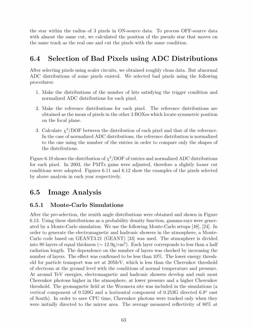
the star within the radius of 3 pixels in ON-source data. To process OFF-source datawith almost the same cut, we calculated the position of the pseudo star that moves onthe same track as the real one and cut the pixels with the same condition.

6.4 Selection of Bad Pixels using ADC Distributions

After selecting pixels using scaler circuits, we obtained roughly clean data. But abnormalADC distributions of some pixels existed. We selected bad pixels using the followingprocedures:

1. Make the distributions of the number of hits satisfying the trigger condition andnormalized ADC distributions for each pixel.

2. Make the reference distributions for each pixel. The reference distributions areobtained as the mean of pixels in the other 3 BOXes which locate symmetric positionon the focal plane.

3. Calculate χ2/DOF between the distribution of each pixel and that of the reference.In the case of normalized ADC distributions, the reference distribution is normalizedto the one using the number of the entries in order to compare only the shapes ofthe distributions.

Figure 6.10 shows the distribution of χ2/DOF of entries and normalized ADC distributionsfor each pixel. In 2003, the PMTs gains were adjusted, therefore a slightly looser cutconditions were adopted. Figures 6.11 and 6.12 show the examples of the pixels selectedby above analysis in each year respectively.

6.5 Image Analysis

6.5.1 Monte-Carlo Simulations

After the pre-selection, the zenith angle distributions were obtained and shown in Figure6.13. Using these distributions as a probability density function, gamma-rays were gener-ated by a Monte-Carlo simulation. We use the following Monte-Carlo setups [48], [24]. Inorder to generate the electromagnetic and hadronic showers in the atmosphere, a Monte-Carlo code based on GEANT3.21 (GEANT) [33] was used. The atmosphere is dividedinto 80 layers of equal thickness (∼ 12.9g/cm2). Each layer corresponds to less than a halfradiation length. The dependence on the number of layers was checked by increasing thenumber of layers. The effect was confirmed to be less than 10%. The lower energy thresh-old for particle transport was set at 20MeV, which is less than the Cherenkov thresholdof electrons at the ground level with the conditions of normal temperature and pressure.At around TeV energies, electromagnetic and hadronic showers develop and emit mostCherenkov photons higher in the atmosphere, at lower pressure and a higher Cherenkovthreshold. The geomagnetic field at the Woomera site was included in the simulations (avertical component of 0.520G and a horizontal component of 0.253G directed 6.8o eastof South). In order to save CPU time, Cherenkov photons were tracked only when theywere initially directed to the mirror area. The average measured reflectivity of 80% at

63

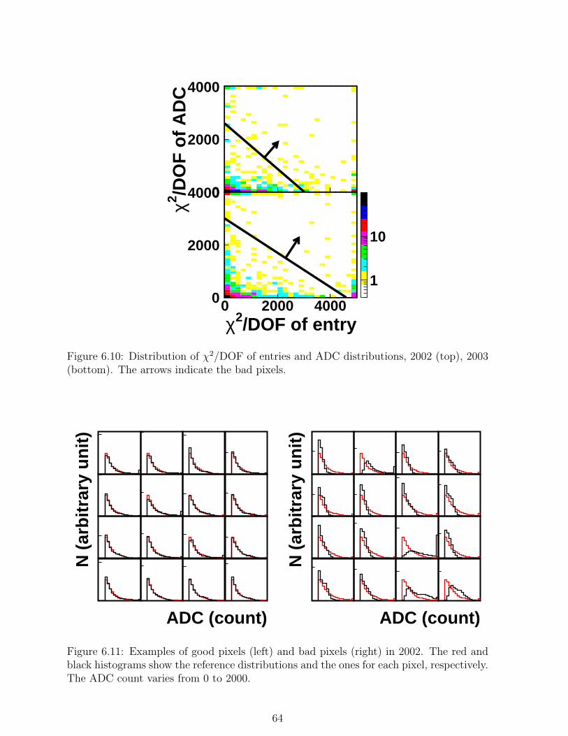
0

2000

4000

0 2000 4000entry vs adc on χ2/N

χ2 /DO

F o

f A

DC

0

2000

4000

0 2000 4000

1

10

entry vs adc on χ2/N

χ2/DOF of entry

Figure 6.10: Distribution of χ2/DOF of entries and ADC distributions, 2002 (top), 2003(bottom). The arrows indicate the bad pixels.

adc

0

10000

0 2000adc

0

10000

0 2000adc

0

10000

0 2000adc

05000

0 2000

ADC (count)

N (

arb

itra

ry u

nit

)

adc

0

10000

0 2000adc

0

5000

0 2000adc

0

5000

0 2000adc

0

5000

0 2000

adc

0

5000

0 2000adc

0

5000

0 2000adc

0

5000

0 2000adc

0

5000

0 2000

adc

0

10000

0 2000adc

0

10000

0 2000adc

0

10000

0 2000adc

0

10000

0 2000

adc

0

5000

0 2000adc

0

5000

0 2000adc

0

5000

0 2000adc

0

5000

0 2000

ADC (count)

N (

arb

itra

ry u

nit

)

adc

0

5000

0 2000adc

0

5000

0 2000adc

0

5000

0 2000adc

0

5000

0 2000

adc

0

10000

0 2000adc

0

5000

0 2000adc

0

10000

0 2000adc

0

2500

0 2000

adc

0

5000

0 2000adc

0

5000

0 2000adc

0

2000

0 2000adc

0

2000

0 2000

Figure 6.11: Examples of good pixels (left) and bad pixels (right) in 2002. The red andblack histograms show the reference distributions and the ones for each pixel, respectively.The ADC count varies from 0 to 2000.

64

adc

0

10000

0 2000adc

0

10000

0 2000adc

0

10000

0 2000adc

0

10000

0 2000

ADC (count)

N (

arb

itra

ry u

nit

)

adc

0

10000

0 2000adc

0

10000

0 2000adc

0

10000

0 2000adc

0

10000

0 2000

adc

0

10000

0 2000adc

0

10000

0 2000adc

0

10000

0 2000adc

0

10000

0 2000

adc

0

10000

0 2000adc

0

10000

0 2000adc

0

10000

0 2000adc

0

10000

0 2000

adc

05000

0 2000adc

0

10000

0 2000adc

0

10000

0 2000adc

0

10000

0 2000

ADC (count)N

(ar

bit

rary

un

it)

adc

0

10000

0 2000adc

0

10000

0 2000adc

0

10000

0 2000adc

0

10000

0 2000

adc

0

10000

0 2000adc

0

10000

0 2000adc

0

10000

0 2000adc

0

5000

0 2000

adc

0

5000

0 2000adc

0

10000

0 2000adc

0

5000

0 2000adc

0

2000

0 2000

Figure 6.12: Examples of good pixels (left) and bad pixels (right) in 2003.

zenith

0

20000

40000

60000

10 20 30 40Zenith angle (degree)

Tim

e (s

ec)

zenith

0

20000

40000

60000

80000

10 20 30 40Zenith angle (degree)

Tim

e (s

ec)

Figure 6.13: Zenith angle distributions in 2002 (top) and 2003 (bottom). The mean zenithangle is 18.3

65

400nm and its wavelength dependence [52] and the measured PMT quantum efficiencywere multiplied by the Frank-Tamm equation to derive the total amount of light andits wavelength dependence. A Rayleigh scattering length of 2970(λ/400 nm) (g/cm2) [9]was used in transport to the ground. When Rayleigh scattering occurred, we treated itas absorption. No Mie scattering was included in this study. The contribution of Miescattering is thought to be at most the 10-20% level. We therefore consider this studyto have uncertainty of at least this level. The diameter of each spherical mirror segmentis 80cm. We assume a Gaussian blur spot of 0.1o [52]. In addition, some mirrors werelost in 2002. This effect was taken into account. The simulated electric noise was added.The timing responses were smeared using a Gaussian of 4ns. NSB photons from doubleJelly’s value of 2.55× 10−4 ergs/cm2/s/str (430-550nm) [50] were also added. Electricsaturation was also taken into account. Finally gamma-rays between 100GeV and 20TeVwere generated assuming the point source and the power law spectrum with index of −2.5(Crab-like). The information of ADCs and TDCs from the simulation were obtained. Weselected gamma-ray event with the same clustering as the experimental data. Calculatingthe dead times on pixels due to scaler cut in experimental data, pixels of the simulationdata were randomly cut using the dead time table as probabilities. Using the integralobservation time for the star of the magnitude 4.1 shown in Figure 6.8 as probabilities,we put the pseudo star position randomly in the Monte Carlo data analysis and cut pixelsaround it within the radius of 3 pixels in order to assume the same live time in both ON,OFF, and Monte Carlo data.

6.5.2 Image Analysis using Likelihood Method

After the previous analysis, the events with the sum of ADC value in the cluster (ADCsum) of more than 1700 were remained. It was difficult to determine the shape of suchevents and also to discriminate between gamma-rays and cosmic rays. Then the stan-dard shape parameters: Width, Length, Distance, and Asymmetry were calculated. Thedistributions of these parameters are shown in Figure 6.14 From above distributions, theevents with 0.2 < Distance < 1.2 were rejected. The Width and Length were used as aLikelihood-ratio described later. We used Eratio defined as follows:

Eratio =ADC sum (the other clusters)

ADC sum (maximum ADC sum cluser)

The distributions of Eratio are shown in Figure 6.15. The gamma-ray events tend tohave only one cluster. Therefore Eratio < 0.1 was adopted. As an indicator of gamma-ray-like events, the Likelihood-ratio (Lratio) was used [23], [24]. Figure 6.16 shows thedistributions of Width and Length as a function of ADC sum. The OFF-source data aremainly protons after the rejection of NSBs. Figure 6.17 shows the image parameters ofthe OFF-source data and the Monte-Carlo simulations of protons. The distributions forthe Monte-Carlo simulations are almost the same as the OFF-source data. However, thereare the differences due to the difficulty in generating hadronic showers by GEANT3.21and the simplifications of the Monte-Carlo simulations. We, therefore, adopted the OFF-source data as a background. From the distributions shown in Figure 6.16, ProbabilityDensity Function (PDF) were derived for both gamma-rays and cosmic rays in variousenergy bands. Figure 6.18 shows the PDFs normalized to unity obtained from Figure6.16. These are dependent on energy. Probability (L) was obtained by multiplying PDF

66

width

02000400060008000

100001200014000

0 0.1 0.2Width ÿ(degree)

N (

arb

itra

ry u

nit

)

length

02000400060008000

1000012000140001600018000

0 0.2 0.4Length ÿ(degree)

distance

0500

10001500200025003000350040004500

0 0.5 1Distance ÿ(degree)

N (

arb

itra

ry u

nit

)

asymmetry

0250050007500

100001250015000175002000022500

-2 -1 0 1 2Asymmetry ÿ(degree)

Figure 6.14: Distributions of Width, Length, Distance, and Asymmetry. The blank his-tograms are the OFF-source data. The hatched histograms are the gamma-rays generatedfrom Monte-Carlo simulations.

Eratio

10 2

10 3

10 4

10 5

10-2

10-1

1Eratio

N

Figure 6.15: Eratio distributions. The blank histograms are the OFF-source data. Thehatched histograms are the gamma-rays generated from Monte-Carlo simulations.

67

0

0.1

0.2

0.3

0.4

0.5

3 4 5 6

sumadc vs wid

Log10 (ADC sum)

Wid

th (

deg

ree)

0

0.2

0.4

0.6

0.8

1

3 4 5 6

sumadc vs len

Log10 (ADC sum)

Len

gth

(d

egre

e)Figure 6.16: Correlations between Hillas parameters (Width and Length) and the loga-rithm of ADC sum. The plotted data are the OFF-source data. The contour are thegamma-rays generated from Monte-Carlo simulations.

(Width) by PDF (Length) in Figure 6.16. In order to obtain a parameter normalized tounity as a indicator of gamma-ray-like events, Lratio is defined as follows:

Lratio =L (gamma− ray)

L (gamma− ray) + L (proton)

Figure 6.19 shows the distributions of Lratio. In order to maximize the statistical signifi-cance of gamma-ray signal, we investigated the figure of merit (FOM); the ratio betweenthe number of the gamma-ray signal of the Monte-Carlo simulation and the square rootof the number of entries of OFF-source data. Figure 6.20 shows the FOM versus Lratio

cut. The acceptance which is normalized to 1 at a cut value of 0 is also shown by thedashed line. The higher cut values lead to a higher statistical significance and a smalleracceptance. we adopted a value of 0.4 for Lratio.

Before investigating gamma-ray signals, we checked the α distributions of OFF-sourcedata. α distribution in 2002 was a slightly slanting. Using χ2/DOF between the α distri-bution in OFF-source data and the flat α distribution normalized to the OFF-source databy the number of the events, we found the pixels which distorted α distributions. Figure6.21 shows the α distributions of OFF-source data in 2002 before and after removing thebad pixels. Flatter α distribution was achieved. Figure 6.22 shows the α distributionsof the OFF-source data and the Monte-Carlo simulations of protons after the likelihoodcut. The α distribution of the OFF-source data was not still flat. The α distribution ofthe simulation, however, was also not flat because of the geometry of the camera and thepixel cut due to the noises and was almost the same as that of the OFF-source data.

68

width vs log ADCsum

05000

100001500020000

0 0.2 0.4Width ÿ(degree)

N (

arb

itra

ry)

length vs log ADCsum

0

10000

20000

0 0.5 1Length ÿ(degree)

distance vs log ADCsum

02000400060008000

0 1Distance ÿ(degree)

N (

arb

itra

ry)

asymmetry vs log ADCsum

0

5000

10000

-2 0 2Asymmetry ÿ(degree)

width vs log ADCsum

0100002000030000

0 0.2 0.4Width ÿ(degree)

N (

arb

itra

ry)

length vs log ADCsum

0

10000

20000

30000

0 0.5 1Length ÿ(degree)

distance vs log ADCsum

05000

1000015000

0 1Distance ÿ(degree)

N (

arb

itra

ry)

asymmetry vs log ADCsum

0

10000

20000

-2 0 2Asymmetry ÿ(degree)

Figure 6.17: Image parameters of the OFF-source data (blank histograms) and the Monte-Carlo simulations of protons (hatched areas). The log (ADCsum)10 of less than 3.7 (up-per) and more than 3.7 (lower), respectively. The protons were generated with the power-law spectrum. The spectral index was −2.7.

69

sumadc vs wid

0

0.05

0.1

0.15

0.2

0 0.1 0.2 0.3 0.4 0.5Width ÿ(degree)

N

sumadc vs len

0

0.05

0.1

0.15

0.2

0 0.2 0.4 0.6 0.8 1Length ÿ(degree)

N

sumadc vs wid

0

0.1

0.2

0 0.1 0.2 0.3 0.4 0.5Width ÿ(degree)

N

sumadc vs len

0

0.1

0.2

0 0.2 0.4 0.6 0.8 1Length ÿ(degree)

N

Figure 6.18: Probability Density Functions normalized to unity. Those of Width andLength with log (ADCsum)10 of 3.6-3.8 (upper) and 4.4-4.6 (lower), respectively. Theblank histograms are OFF-source data. The hatched areas are from the gamma-raysimulations.

70

likelihood ratio

10 2

10 3

10 4

0 0.2 0.4 0.6 0.8 1Lratio

N

00.10.20.30.40.50.60.70.80.91

0 0.2 0.4 0.6 0.8 1

likelihood ratio

10 2

10 3

10 4

10 5

0 0.2 0.4 0.6 0.8 1Lratio

N00.10.20.30.40.50.60.70.80.91

0 0.2 0.4 0.6 0.8 1

Figure 6.19: Distributions of Likelihood-ratio (Lratio). The blank histograms are obtainedfor the OFF-source data and the hatched ones are for the gamma-ray Monte-Carlo sim-ulation. The number of gamma-rays from the Monte-Carlo simulations were normalizedto that of the OFF-source data.

Figure 6.20: Figure of merit (FOM) versus Likelihood-ratio (Lratio) cut for the combineddata is shown by the dashed line. The acceptance versus Likelihood-ratio cut is alsoshown by the dotted line. The acceptance is normalized to 1 at a cut value of 0. TheFOM multiplied by the acceptance is shown by the solid line.

71

alpha

0

1000

2000

3000

4000

0 20 40 60 80α(degree)

Nu

mb

er o

f ev

ents

per

5o

alpha

0

1000

2000

3000

4000

0 20 40 60 80α(degree)

Nu

mb

er o

f ev

ents

per

5o

Figure 6.21: Distributions of α for OFF-source data in 2002. The horizontal lines werenormalized to the α distributions by the number of events. χ2/DOF between the αdistribution and the horizontal line before removing bad pixels (upper) was 17.6. χ2/DOFafter removing bad pixels (lower) was 6.2.

alpha

0

1000

2000

3000

0 20 40 60 80α(degree)

Nu

mb

er o

f ev

ents

per

5o

Figure 6.22: Distributions of α for the OFF-source data (solid line) and the Monte-Carlo simulations of protons (dotted line) after the likelihood cut. The histogram of thesimulation was normalized to the OFF-source data by the number of the events. Theprotons were generated with the power-law spectrum. The spectral index was −2.7.

72

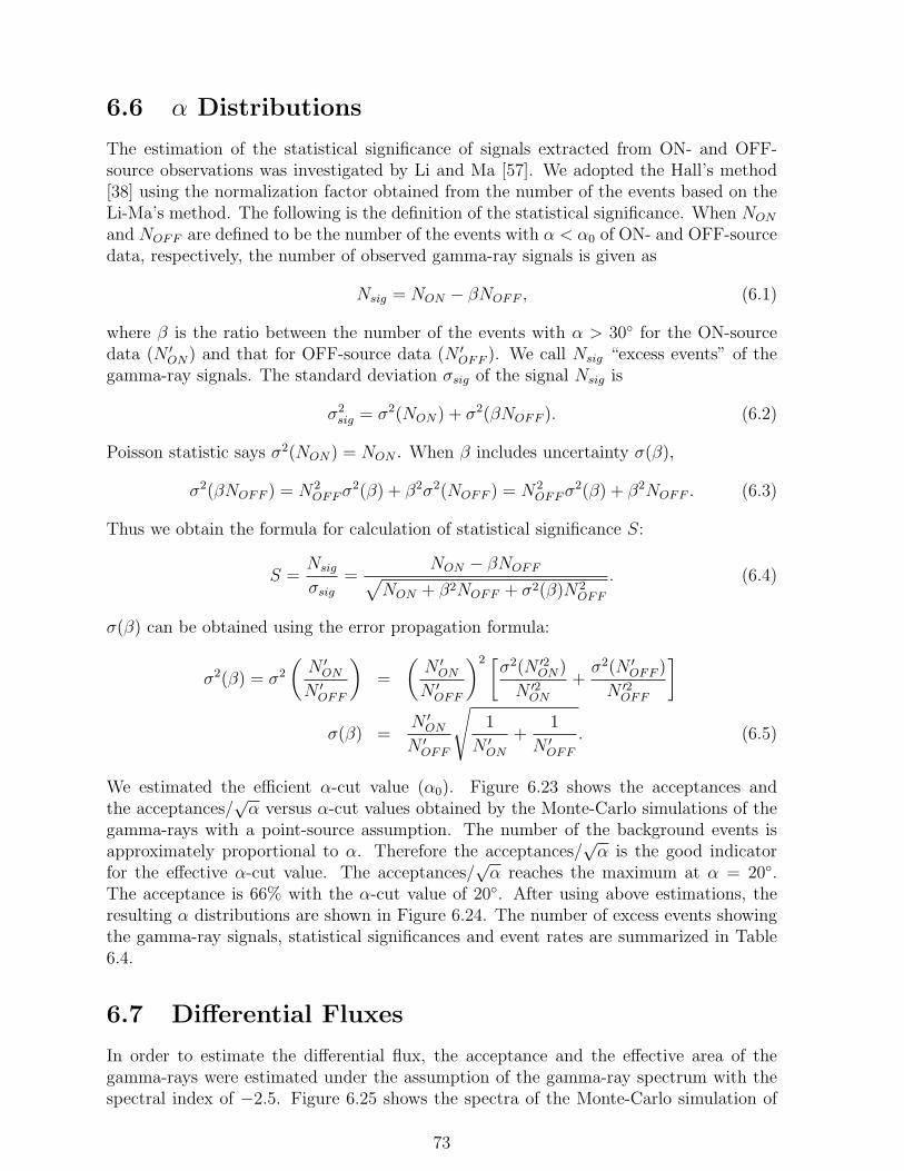
6.6 α Distributions

The estimation of the statistical significance of signals extracted from ON- and OFF-source observations was investigated by Li and Ma [57]. We adopted the Hall’s method[38] using the normalization factor obtained from the number of the events based on theLi-Ma’s method. The following is the definition of the statistical significance. When NON

and NOFF are defined to be the number of the events with α < α0 of ON- and OFF-sourcedata, respectively, the number of observed gamma-ray signals is given as

Nsig = NON − βNOFF , (6.1)

where β is the ratio between the number of the events with α > 30 for the ON-sourcedata (N ′

ON) and that for OFF-source data (N ′OFF ). We call Nsig “excess events” of the

gamma-ray signals. The standard deviation σsig of the signal Nsig is

σ2sig = σ2(NON) + σ2(βNOFF ). (6.2)

Poisson statistic says σ2(NON) = NON . When β includes uncertainty σ(β),

σ2(βNOFF ) = N2OFF σ2(β) + β2σ2(NOFF ) = N2

OFF σ2(β) + β2NOFF . (6.3)

Thus we obtain the formula for calculation of statistical significance S:

S =Nsig

σsig

=NON − βNOFF√

NON + β2NOFF + σ2(β)N2OFF

. (6.4)

σ(β) can be obtained using the error propagation formula:

σ2(β) = σ2

(N ′

ON

N ′OFF

)=

(N ′

ON

N ′OFF

)2 [σ2(N ′2

ON)

N ′2ON

+σ2(N ′

OFF )

N ′2OFF

]

σ(β) =N ′

ON

N ′OFF

√1

N ′ON

+1

N ′OFF

. (6.5)

We estimated the efficient α-cut value (α0). Figure 6.23 shows the acceptances andthe acceptances/

√α versus α-cut values obtained by the Monte-Carlo simulations of the

gamma-rays with a point-source assumption. The number of the background events isapproximately proportional to α. Therefore the acceptances/

√α is the good indicator

for the effective α-cut value. The acceptances/√

α reaches the maximum at α = 20.The acceptance is 66% with the α-cut value of 20. After using above estimations, theresulting α distributions are shown in Figure 6.24. The number of excess events showingthe gamma-ray signals, statistical significances and event rates are summarized in Table6.4.

6.7 Differential Fluxes

In order to estimate the differential flux, the acceptance and the effective area of thegamma-rays were estimated under the assumption of the gamma-ray spectrum with thespectral index of −2.5. Figure 6.25 shows the spectra of the Monte-Carlo simulation of

73

0

0.2

0.4

0.6

0.8

1

0 10 20 30α cut (degree)

Acc

epta

nce

0

0.05

0.1

0.15

0.20 10 20 30

Acc

epta

nce

/√ α

Acceptance

Acceptance/√ α

Figure 6.23: Acceptances (open circles) and the acceptances/√

α (closed circles) versusα-cut values obtained by the Monte-Carlo simulations of the gamma-rays with a point-source assumption. The α distribution after likelihood cut was used. The acceptanceswere normalized by the total number of events before the α cut. The number of thebackground events is approximately proportional to α.

Observation date Excess events Statistical significance Events/min.16-Dec. 2001 – 15-Feb. 2002 887±164 5.4 0.42±0.0805-Jan. 2003 – 28-Feb. 2003 966±175 5.5 0.44±0.08Combined 1658±241 6.8 0.39±0.06

Table 6.4: Number of excess events showing the gamma-ray signals, statistical signif-icances and event rates assuming the spectral index of the Monte-Carlo simulation is−2.5.

74

alpha

0

2000

4000

6000

0 50Nu

mb

er o

f ev

ents

per

5o

alpha

0

2000

4000

6000

0 50

alpha

0

2000

4000

6000

0 50α(degree)

Figure 6.24: Distributions of α: 2002 (left), 2003 (middle), and the combined (right).The points with statistical errors show the α distributions of the ON-source data. Thehatched areas show that of the OFF-source data. The OFF-source data were normalizedby the ratio between the number of the events with α > 30 for the ON-source data andthat for OFF-source data.

75

Figure 6.25: Spectra of the Monte-Carlo simulation of gamma-rays under the assumptionof the spectrum with the spectral index of −2.5 as a function of energy (left) and ADCsum (right) which is proportional to the energy. The blank histogram shows the spectrumof the events which were generated by the power-law spectrum with the spectral indexof −2.5 assuming the point source. The hatched area shows the spectrum of the eventsafter the α cut.

gamma-rays as a function of energy (left) and ADC sum (right) which is proportional tothe energy. Using the left in Figure 6.25, the effective area S(El, Eu) between the lowerboundary of the energy El and the upper boundary of the energy Eu is defined as follows:

S(El, Eu) ≡ S0A(El, Eu), (6.6)

where S0 and A(El, Eu) are the area which was calculated by averaging the areas wherethe gamma-rays were generated dependent on the elevation and the acceptance which isthe ratio between the number of the accepted gamma-ray events and that of the generatedgamma-ray events with the same energy range. The right of Figure 6.26 shows the effectiveareas of gamma-rays as a function of energy and the effective areas multiplied by E−2.5.However the values of the left in Figure 6.26 cannot be used because they are the effectiveareas as a function of energy. The energy was not clear for the experimental data. Thuswe used ADC sum instead of energy. We used the acceptance as a function of ADC sumA′(xl, xu) , i.e. the ratio between the number of the accepted gamma-ray events in xl

< ADC sum < xu and that of the total generated gamma-ray events obtained from theright in Figure 6.26. We obtained α distributions in various ADC-sum regions. The αdistributions in various ADC sum regions are shown in Figure 6.27. The value of theexcess events Nsig(xl, xu) in the region of ADC sum between xl and xu was obtained fromthese distributions. In order to estimate the mean energies of the excess events of thegamma-ray signals, we used the data of the gamma-rays generated from the Monte-Carlosimulation. Figure 6.28 shows the correlation between the energy and the ADC sum of thegamma-ray events from the Monte-Carlo simulation. Figure 6.29 shows the distributionsof the energies of the gamma-rays in each region of ADC sum which were obtained fromFigure 6.28. The mean energy E(xl, xu) of the excess events in the region of ADC sumbetween xl and xu was estimated from the mean of each distribution in Figure 6.29. The

76

10 7

10 8

10 9

1 10Energy (TeV)

Eff

ecti

ve a

rea

(cm

2 )

10 7

10 8

10 9

2.5 3 3.5 4

10 7

10 8

10 9

1 10Energy (TeV)

Eff

ecti

ve a

rea×

E-2

.5(c

m2 T

eV-2

.5)

10 7

10 8

10 9

2.5 3 3.5 4

Figure 6.26: Effective areas of the gamma-rays under the assumption of the spectrumwith the spectral index of −2.5 as a function of energy (left); the effective areas afterpre-selection (the black squares), those after the distance cut (the black triangles), thoseafter the Likelihood-ratio cut (the blank circles), and those with α < 20 (the blanksquares). The effective area for the Whipple telescope is shown by the dashed line (afterthe distance cut) [60]. The effective areas multiplied by E−2.5 are shown in the right figurein order to indicate the threshold of the CANGAROO-II 10-m telescope.

77

Figure 6.27: α distributions for each ADC sum: less than 2500 (upper left), 2500-3500(upper right), 3500-7000 (lower left), and more than 7000 (lower right), respectively. Thepoints with statistical errors show the α distributions of the ON-source data. The hatchedareas show that of the OFF-source data. The OFF-source data were normalized by theratio between the number of the events with α > 30 for the ON-source data and that forOFF-source data.

78

Figure 6.28: Correlation between the energy and the ADC sum of the gamma-ray eventsfrom the Monte-Carlo simulation.

following is the method to estimate the differential flux using the above values. At first, weassumed the differential flux of the gamma-rays of the Monte-Carlo simulation as follows:

dF

dE=

1

Emax

(E

Emax

)−α

, (6.7)

where Emax, E, and α are the maximum energy of the generated gamma-rays, the energyof the gamma-rays, and the spectral index. The expected total number of the incidentgamma-ray events within the area S0 N tot

MC is given as

N totMC = S0TON

∫ Emax

Emin

dF

dEdE

=S0TON

1− α

1−

(Emin

Emax

)−α+1

, (6.8)

where TON and Emin are the observation time of ON-source data and the minimum energyof the generated gamma-rays. The expected number of the accepted gamma-rays betweenxl and xu, NMC(xl, xu), is given as

NMC(xl, xu) = N totMCA′(xl, xu). (6.9)

The real differential flux at the energy E(xl, xu) can be estimated using the ratio betweenNsig(xl, xu) and NMC(xl, xu) as

dF

dE(xu, xl) =

Nsig(xl, xu)

NMC(xl, xu)

[dF

dE

]

E(xl,xu)

=Nsig(xl, xu)

S0A′(xl, xu)TON

1− α

E−α+1max − E−α+1

min

E(xl, xu)−α. (6.10)

79

Figure 6.29: Distributions of the energies of the gamma-rays in each region of ADC sum:less than 2500 (upper left), 2500-3500 (upper right), 3500-7000 (lower left), and morethan 7000 (lower right), respectively.

Energy (TeV) Excess event Acceptance Differential flux (cm−2s−1TeV −1)0.49 576 ± 121 3.19 × 10−3 9.47 ± 1.99 × 10−11

0.56 409 ± 113 3.36 × 10−3 4.57 ± 1.26 × 10−11

0.79 381 ± 137 7.32 × 10−3 8.33 ± 3.00 × 10−12

2.39 277 ± 109 1.12 × 10−2 2.47 ± 0.98 × 10−13

Table 6.5: Summary of the the number of excess events Nsig(xl, xu) with the statisti-cal errors, the acceptances A′(xl, xu) and the differential fluxes dF/dE(xl, xu) with thestatistical errors. The statistical errors of the differential fluxes were estimated by calcu-lating the flux with exchanging the number of excess event into the statistical error. Thedefinition of A′(xl, xu) is described in the text.

80

The differential fluxes are summarized in Table 6.5, where S0, TON , α, Emin, and Emax are2.09×109cm2, 2.58×105s, −2.5, 100GeV, and 20TeV, respectively. The differential fluxeswith only the statistical errors are plotted in Figure 6.30. However the obtained index of

Figure 6.30: Differential fluxes with the statistical errors. The flux with the combineddata of 2002 and 2003 is shown. The solid line shows the flux of Crab nebula [2].

the spectrum was −3.9±0.5. The iteration of changing the spectral index of the Monte-Carlo simulations of gamma-rays was carried out until the obtained index converged atthe assumed one. Figure 6.31 shows the assumed indices of the gamma-ray Monte-Carlosimulation and the ratio of the indices between the assumed spectrum and the obtainedspectrum. The index converged at −4.5±0.5.

81

-5-4-3-2

0 2 4 6

α IN

0.51

1.52

0 2 4 6Times

α OU

T/α

IN

Figure 6.31: Assumed indices of the gamma-ray Monte-Carlo simulation and the ratio ofthe indices between the assumed spectrum (αIN) and the obtained spectrum (αOUT ).

82

Chapter 7

Results

7.1 α Distributions

The resulting α distributions after the iteration are shown in Figure 7.1. The number

alpha

0

2000

4000

6000

0 50Nu

mb

er o

f ev

ents

per

5o

alpha

0

2000

4000

6000

0 50

alpha

0

2000

4000

6000

0 50α(degree)

Figure 7.1: Distributions of α after the iteration: 2002 (left), 2003 (middle), and thecombined (right). The points with statistical errors show the α distributions of the ON-source data. The hatched areas show that of the OFF-source data. The OFF-sourcedata were normalized by the ratio between the number of events with α > 30 for theON-source data and that for OFF-source data.

.

of excess events showing the gamma-ray signals, statistical significances and event ratesare summarized in Table 7.1. We also estimated systematic errors of α distributions in

83

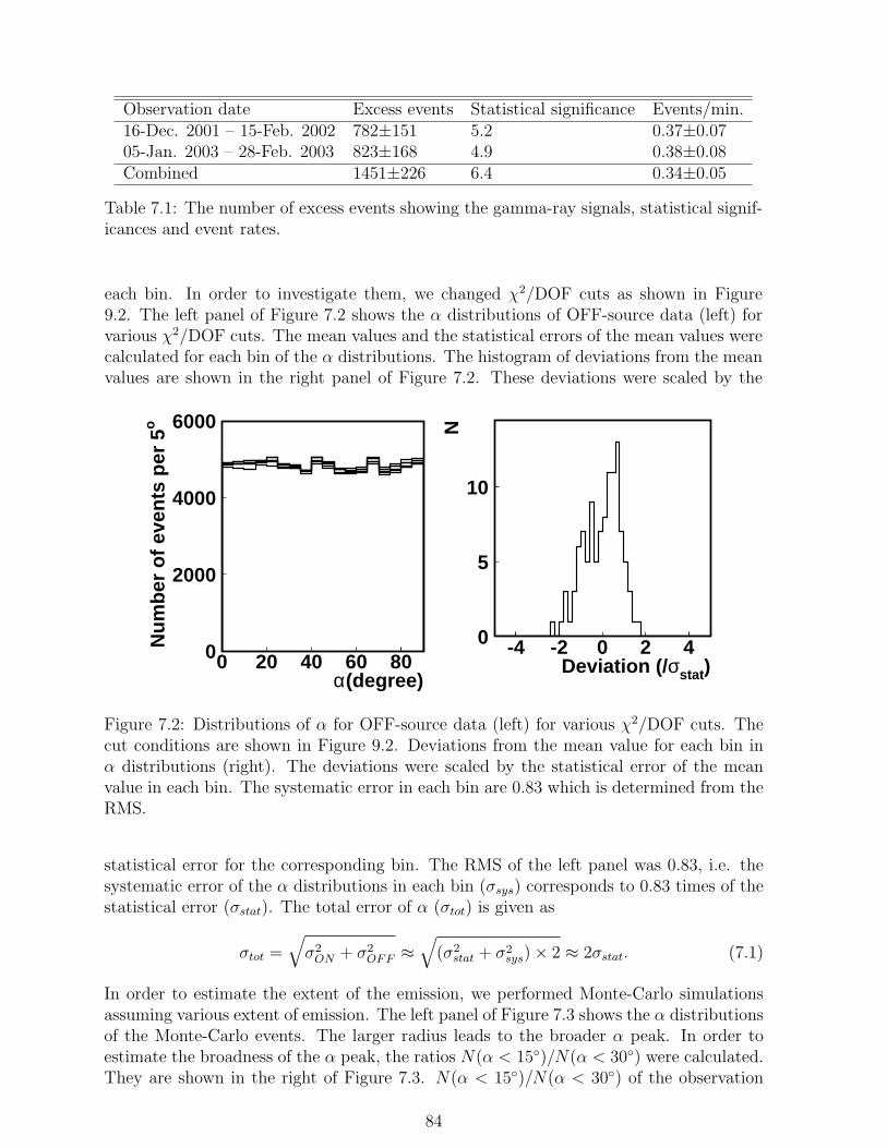
Observation date Excess events Statistical significance Events/min.16-Dec. 2001 – 15-Feb. 2002 782±151 5.2 0.37±0.0705-Jan. 2003 – 28-Feb. 2003 823±168 4.9 0.38±0.08Combined 1451±226 6.4 0.34±0.05

Table 7.1: The number of excess events showing the gamma-ray signals, statistical signif-icances and event rates.

each bin. In order to investigate them, we changed χ2/DOF cuts as shown in Figure9.2. The left panel of Figure 7.2 shows the α distributions of OFF-source data (left) forvarious χ2/DOF cuts. The mean values and the statistical errors of the mean values werecalculated for each bin of the α distributions. The histogram of deviations from the meanvalues are shown in the right panel of Figure 7.2. These deviations were scaled by the

0

2000

4000

6000

0 20 40 60 80α(degree)

Nu

mb

er o

f ev

ents

per

5o

systematics of alpha

0

5

10

-4 -2 0 2 4Deviation (/σstat)

N

Figure 7.2: Distributions of α for OFF-source data (left) for various χ2/DOF cuts. Thecut conditions are shown in Figure 9.2. Deviations from the mean value for each bin inα distributions (right). The deviations were scaled by the statistical error of the meanvalue in each bin. The systematic error in each bin are 0.83 which is determined from theRMS.

statistical error for the corresponding bin. The RMS of the left panel was 0.83, i.e. thesystematic error of the α distributions in each bin (σsys) corresponds to 0.83 times of thestatistical error (σstat). The total error of α (σtot) is given as

σtot =√

σ2ON + σ2

OFF ≈√

(σ2stat + σ2

sys)× 2 ≈ 2σstat. (7.1)

In order to estimate the extent of the emission, we performed Monte-Carlo simulationsassuming various extent of emission. The left panel of Figure 7.3 shows the α distributionsof the Monte-Carlo events. The larger radius leads to the broader α peak. In order toestimate the broadness of the α peak, the ratios N(α < 15)/N(α < 30) were calculated.They are shown in the right of Figure 7.3. N(α < 15)/N(α < 30) of the observation

84

alpha

0

20

40

60

80

0 20 40 60 80α (degree)

Nu

mb

er o

f ev

ents

per

5o

0.5

0.6

0.7

0.8

0 0.2 0.4Radius (degree)

N(α

<15o

)/N

(α<3

0o)

WithinPSF

Figure 7.3: Distributions of α for the Monte-Carlo simulations assuming the emission isextended and the spectral index is −4.5 (left). The morphologies of the diffuse emissionswere the circles with the radius of 0, 0.1, 0.2, 0.3, 0.4, and 0.5 degree, respectively. Thelarger radius leads to the broader α peak. Ratio N(α < 15)/N(α < 30) with the sameassumptions for the simulations (right). The points are the Monte-Carlo simulations withthe assumptions of the diffuse emissions with the radius of 0, 0.1, 0.2, 0.3, 0.4, and 0.5degree, respectively. The solid line and the hatched area show N(α < 15)/N(α < 30)and the statistical error which were obtained from our data. The dashed line shows thePoint Spread Function of the CANGAROO-II 10-m telescope.

85

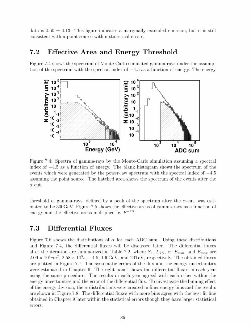
data is 0.60 ± 0.13. This figure indicates a marginally extended emission, but it is stillconsistent with a point source within statistical errors.

7.2 Effective Area and Energy Threshold

Figure 7.4 shows the spectrum of Monte-Carlo simulated gamma-rays under the assump-tion of the spectrum with the spectral index of −4.5 as a function of energy. The energy

Figure 7.4: Spectra of gamma-rays by the Monte-Carlo simulation assuming a spectralindex of −4.5 as a function of energy. The blank histogram shows the spectrum of theevents which were generated by the power-law spectrum with the spectral index of −4.5assuming the point source. The hatched area shows the spectrum of the events after theα cut.

threshold of gamma-rays, defined by a peak of the spectrum after the α-cut, was esti-mated to be 300GeV. Figure 7.5 shows the effective areas of gamma-rays as a function ofenergy and the effective areas multiplied by E−4.5.

7.3 Differential Fluxes

Figure 7.6 shows the distributions of α for each ADC sum. Using these distributionsand Figure 7.4, the differential fluxes will be discussed later. The differential fluxesafter the iteration are summarized in Table 7.2, where S0, TON , α, Emin, and Emax are2.09× 109cm2, 2.58× 105s, −4.5, 100GeV, and 20TeV, respectively. The obtained fluxesare plotted in Figure 7.7. The systematic errors of the flux and the energy uncertaintieswere estimated in Chapter 9. The right panel shows the differential fluxes in each yearusing the same procedure. The results in each year agreed with each other within theenergy uncertainties and the error of the differential flux. To investigate the binning effectof the energy division, the α distributions were created in finer energy bins and the resultsare shown in Figure 7.8. The differential fluxes with more bins agree with the best fit lineobtained in Chapter 9 later within the statistical errors though they have larger statisticalerrors.

86

10 7

10 8

10 9

1 10Energy (TeV)

Eff

ecti

ve a

rea

(cm

2 )

10 7

10 8

10 9

2.5 3 3.5 4

10 610 710 810 9

10 1010 11

1 10Energy (TeV)

Eff

ecti

ve a

rea×

E-4

.5(c

m2 T

eV-4

.5)

10 610 710 810 9

10 1010 11

2.5 3 3.5 4

Figure 7.5: Effective areas of the gamma-rays under the assumption of the spectrum withthe spectral index of −4.5 as a function of energy (left); the effective areas after pre-selection (the black squares), those after the distance cut (the black triangles), those afterthe Likelihood-ratio cut (the blank circles), and those with α < 20 (the blank squares).The effective area for the Whipple telescope is shown by the dashed line (after the distancecut) [60]. The effective areas multiplied by E−4.5 are shown in the right figure in order toindicate the threshold of the CANGAROO-II 10-m telescope.

Energy (TeV) Excess event Acceptance Differential flux (cm−2s−1TeV −1)0.31 512 ± 113 5.25 × 10−4 3.87 ± 0.86 × 10−10

0.37 372 ± 105 4.31 × 10−4 1.61 ± 0.45 × 10−10

0.53 344 ± 133 4.67 × 10−4 2.60 ± 1.01 × 10−11

1.01 218 ± 100 1.78 × 10−4 2.41 ± 1.10 × 10−12

Table 7.2: Summary of the the number of excess events Nsig(xl, xu) with the statisti-cal errors, the acceptances A′(xl, xu) and the differential fluxes dF/dE(xl, xu) with thestatistical errors under the assumption of the spectrum with the spectral index of −4.5. The statistical errors of the differential fluxes were estimated by calculating the fluxwith exchanging the number of excess event into the statistical error. The definition ofA′(xl, xu) is described in the text.

87

Figure 7.6: Distributions of α after the iteration for each ADC sum: less than 2500 (upperleft), 2500-3500 (upper right), 3500-7000 (lower left), and more than 7000 (lower right),respectively. The points with statistical errors show the α distributions of the ON-sourcedata. The hatched areas show that of the OFF-source data. The OFF-source data werenormalized by the ratio between the number of events with α > 30 for the ON-sourcedata and that for OFF-source data.

88

10-15

10-14

10-13

10-12

10-11

10-10

10-9

103

104

Energy(GeV)

Dif

fere

nti

al f

lux(

cm-2

sec-1

TeV

-1)

Crab

Figure 7.7: Differential fluxes with the statistical errors after the iteration. The flux withthe combined data of 2002 and 2003 is shown in the left panel. Those in 2002 (closedcircles) and in 2003 (open circles) are shown in the right panel. The solid line shows theflux of Crab nebula [2].

10-15

10-14

10-13

10-12

10-11

10-10

10-9

103

104

Energy(GeV)

Dif

fere

nti

al f

lux(

cm-2

sec-1

TeV

-1)

Crab

Figure 7.8: Differential fluxes of different binnings. Open circles are the same binnings asFigure 6.30. The differential flux with more binnings is plotted with open squares. Theregions of ADC sum are less than 2300, 2300-3000, 3000-7000, 7000-10000, 10000-15000,15000-28000, 28000-40000, and more than 40000 , respectively. The thick solid line showsthe best fit line obtained in the chapter 9. The arrows show the 2 σ upper limits.

89

7.4 Morphology

The blue contours in Figure 7.9 represent the source morphology obtained from our ob-servations. These contours were obtained from the so-called significance map and are,

134 133 132 131

-47.0

-46.5

-46.0

-45.5

-45.0

134 133 132 131

-47.0

-46.5

-46.0

-45.5

-45.0

134 133 132 131

-47.0

-46.5

-46.0

-45.5

-45.0

134 133 132 131

-47.0

-46.5

-46.0

-45.5

-45.0

134 133 132 131

-47.0

-46.5

-46.0

-45.5

-45.0

134 133 132 131

-47.0

-46.5

-46.0

-45.5

-45.0

134 133 132 131

-47.0

-46.5

-46.0

-45.5

-45.0

134 133 132 131

-47.0

-46.5

-46.0

-45.5

-45.0

134 133 132 131Right Ascension (J2000, degree)

-47.0

-46.5

-46.0

-45.5

-45.0

Dec

linat

ion

(J20

00, d

egre

e)

40%

134 133 132 131

-47.0

-46.5

-46.0

-45.5

-45.0

134 133 132 131

-47.0

-46.5

-46.0

-45.5

-45.0

134 133 132 131

-47.0

-46.5

-46.0

-45.5

-45.0

134 133 132 131

-47.0

-46.5

-46.0

-45.5

-45.0

134 133 132 131

-47.0

-46.5

-46.0

-45.5

-45.0

134 133 132 131

-47.0

-46.5

-46.0

-45.5

-45.0

134 133 132 131

-47.0

-46.5

-46.0

-45.5

-45.0

134 133 132 131

-47.0

-46.5

-46.0

-45.5

-45.0

134 133 132 131Right Ascension (J2000, degree)

-47.0

-46.5

-46.0

-45.5

-45.0

Dec

linat

ion

(J20

00, d

egre

e)

40%

40%

65%

134 133 132 131

-47.0

-46.5

-46.0

-45.5

-45.0

134 133 132 131

-47.0

-46.5

-46.0

-45.5

-45.0

134 133 132 131

-47.0

-46.5

-46.0

-45.5

-45.0

134 133 132 131

-47.0

-46.5

-46.0

-45.5

-45.0

134 133 132 131

-47.0

-46.5

-46.0

-45.5

-45.0

134 133 132 131

-47.0

-46.5

-46.0

-45.5

-45.0

134 133 132 131

-47.0

-46.5

-46.0

-45.5

-45.0

134 133 132 131

-47.0

-46.5

-46.0

-45.5

-45.0

134 133 132 131Right Ascension (J2000, degree)

-47.0

-46.5

-46.0

-45.5

-45.0

Dec

linat

ion

(J20

00, d

egre

e)

40%

65%

Figure 7.9: Significance maps of gamma-ray signal from 2002 observation (top left), 2003one (top right) and combined (bottom). Our observations are shown by the blue contours,which show 40%, 65%, and 80% of the peak weight, respectively. ASCA X-ray images byred contours, and 4850MHz radio by green contours.

therefore, not proportional to gamma-ray flux. The significance map was made fromthe distribution of the significance assuming that each point was a point-source posi-tion. The angular resolution of CANGAROO-II 10-m telescope was estimated as follows[48]. Gamma-rays were generated by the Monte-Carlo simulation with the point-sourceassumption. The excess map was obtained using the same method for obtaining the sig-nificance map. The map was fit to the Gaussian distribution. The PSF was defined asthe standard deviation and estimated to be ∼ 0.24. The significance is proportional tothe intensity only when the acceptance and the background level are uniform in the full

90

FOV. The acceptance is dependent on the offset angle of the assumed source positionfrom the center of the field of view, as shown in Figure 7.10. The center positions of

0

0.25

0.5

0.75

1

0 0.2 0.4 0.6 0.8

Acc

epta

nce

Figure 7.10: Acceptance versus offset angle of the gamma-ray source position from thecenter of the field of view. The acceptance were normalized to that without offset.

excesses coincided with the maximum X-ray point and the radio data. From Figure 7.9,the 65% contour of our data are approximately 0.34 along the major axis and 0.20 alongthe minor axis, respectively. Using these values and the angular resolution, the real sizex [degree], if it is extended, is estimated as

0.34× 0.20 ≈ 0.242 + x2

x ≈ 0.10. (7.2)

91

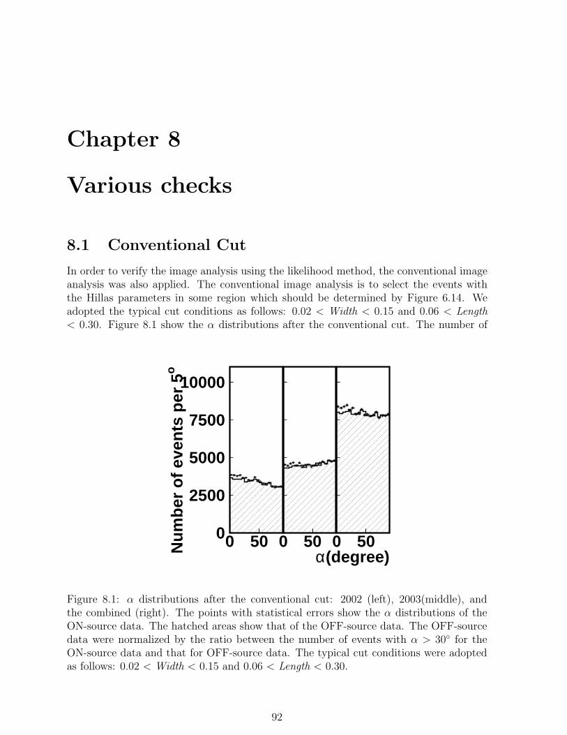
Chapter 8

Various checks

8.1 Conventional Cut

In order to verify the image analysis using the likelihood method, the conventional imageanalysis was also applied. The conventional image analysis is to select the events withthe Hillas parameters in some region which should be determined by Figure 6.14. Weadopted the typical cut conditions as follows: 0.02 < Width < 0.15 and 0.06 < Length< 0.30. Figure 8.1 show the α distributions after the conventional cut. The number of

alpha

0

2500

5000

7500

10000

0 50Nu

mb

er o

f ev

ents

per

5o

alpha

0

2500

5000

7500

10000

0 50

alpha

0

2500

5000

7500

10000

0 50α(degree)

Figure 8.1: α distributions after the conventional cut: 2002 (left), 2003(middle), andthe combined (right). The points with statistical errors show the α distributions of theON-source data. The hatched areas show that of the OFF-source data. The OFF-sourcedata were normalized by the ratio between the number of events with α > 30 for theON-source data and that for OFF-source data. The typical cut conditions were adoptedas follows: 0.02 < Width < 0.15 and 0.06 < Length < 0.30.

92

excess events showing the gamma-ray signals, statistical significances and event rates afterthe conventional cut are summarized in Table 8.1. From these results, we confirmed the

Observation date Excess events Statistical significance Events/min.16-Dec. 2001 – 15-Feb. 2002 908±193 4.7 0.43±0.0905-Jan. 2003 – 28-Feb. 2003 843±222 3.8 0.39±0.10Combined 1453±295 4.9 0.34±0.07

Table 8.1: The number of excess events showing the gamma-ray signals, statistical signif-icances and event rates after the conventional cut.

statistical significance of the detection by the conventional image analysis.There are four reasons why we did not adopt this conventional method and use the

likelihood method. One is the dependence of the Hillas parameters on energy. Sincethe distributions shown in Figure 6.16 are used in the likelihood method, the energydependence is taken into account. The second is the artificial effect. The conventionalcuts on each parameter depend on the cut conditions selected artificially. On the otherhand, the likelihood method avoid the artificial effect except for only one parameter, thelikelihood-ratio. The third is the estimation of the systematic effect. Since the systematiceffect due to the cut condition is only due to the cut condition of the likelihood-ratio, it canbe easily estimated by changing one parameter. The fourth is the figure of merit (FOM)which was defined in the subsection 6.5.2. The FOM of the cut with the likelihood-ratio> 0.4 was about 1.1 times as large as that of the conventional cut which was estimatedusing the gamma-rays of the Monte-Carlo simulations.

If the excess events are gamma-rays, the number of excess events should not be stronglydependent on only one parameter. Figure 8.2 shows the α distributions after various cuts.There was no strong dependence.

8.2 Effects of the Bad Pixel Cut

The selections of bad pixels using the ADC distributions were described in the section6.4. However, distortions of the Hillas parameters and the decrease of the acceptanceof gamma-rays due to the removed pixels should be checked. Figure 8.3 shows the badpixels selected using the ADC distributions. First, the acceptances of gamma-rays wereinvestigated. The upper panel of Figure 8.4 shows the changes of α distributions obtainedby analyzing the data of the Monte-Carlo simulations of gamma-rays. From these figures,the acceptance of gamma-rays before and after selecting the bad pixels were calculated.Table 8.2 summarizes the ratio of the cut pixels and the acceptance of selecting the badpixels using the ADC distributions. More than 70% of the events remained.

Distortions of the Hillas parameters were also investigated. The lower panel of Figure8.4 shows the change of the Length and Width obtained by analyzing the Monte-Carlosimulations of gamma-rays.

93

alpha

0

20000

0 50

Nu

mb

er o

f ev

ents

per

5o

alpha

0

20000

0 50

alpha

0

5000

0 50

α (degree)

Figure 8.2: α distributions: no image analysis (left), only Distance cut (middle), and theDistance cut and the conventional cut using Width and Length (right).

-1

0

1

-1 0 1

-1

0

1

-1 0 1

Figure 8.3: Bad pixels selected using the ADC distributions in 2002 (left) and 2003 (right).

Observation date Ratio of cut pixels (%) Acceptance (%)16-Dec. 2001 – 15-Feb. 2002 23.6 70.505-Jan. 2003 – 28-Feb. 2003 15.6 77.5

Table 8.2: Ratio of the cut pixels and the acceptance of selecting the bad pixels using ADCdistributions. The excess events are counted with α of less than 20. The acceptances arenormalized to that without the cut pixels.

94

alpha

0

10

20

30

40

0 50

α(degree)

N (

arb

itra

ry u

nit

)

alpha

0

20

40

60

0 50α(degree)

N (

arb

itra

ry u

nit

)

width

0

20

40

60

0 0.2 0.4

N (

arb

itra

ry u

nit

)

length

0

20

40

60

0 0.5 1

width

020406080

0 0.2 0.4(degree)Width ÿ

length

020406080

0 0.5 1(degree)Length ÿ

Figure 8.4: Upper figure: the changes of α distributions obtained by analyzing the dataof the Monte-Carlo simulations of gamma-rays in 2002 (left) and 2003 (right). The blankand the dotted histograms are obtained before and after removing bad pixels, respectively.Lower figure: the change of the Width (left) Length (right) obtained by analyzing theMonte-Carlo simulations of gamma-rays in 2002 (upper) and 2003 (lower).

95

8.3 Hillas Parameter Distributions of Excess Events

In order to make a further confirmation that the excess events are the gamma-rays, wecompared the distributions of the Hillas parameters for the excess events with those ofthe gamma-rays generated by the Monte-Carlo simulations. They are shown in Figure8.5. For obtaining each parameter distribution, the reference parameter was not used in

0

0.2

0.4

0.6

0.8

0 0.05 0.1 0.15 0.2(degree)

Sig

nal

yie

ld/T

ota

l

Width ÿ

0

0.1

0.2

0.3

0.4

0.5

0.6

0 0.1 0.2 0.3 0.4(degree)

Sig

nal

yie

ld/T

ota

l

Length ÿ

0

0.1

0.2

0.3

0.4

-1 0 1(degree)

Sig

nal

yie

ld/T

ota

l

Asymmetry ÿ

0

0.1

0.2

0.3

0.4

0.5

0.6

0 0.5 1 1.5(degree)

Sig

nal

yie

ld/T

ota

l

Distance ÿ

Figure 8.5: Distributions of the Hillas parameters for the excess events and the gamma-rays generated by the Monte-Carlo simulations. The points with the statistical error barswere obtained by experimental data. The solid lines were obtained by the Monte-Carlosimulations of gamma-rays with the power-law index of −4.5. The dotted line shows theOFF-source data with α < 20. For obtaining each parameter distribution, the referenceparameter was not used in calculating Lratio.

calculating Lratio. The distributions of the excess events are roughly the same as thoseof the gamma-rays generated by the Monte-Carlo simulations with the spectral index of−4.5.

96

8.4 Crab Analysis

To check the analysis procedure and the calibration, the data of Crab taken in December2000 was analyzed as a standard source. The elevation angle ranged from 34 to 37. Table8.3 summarizes the observation time for Crab nebula before and after the pre-selection.The energy threshold was estimated from simulations to be ≈ 2TeV. The resulting α

TON(min) TOFF(min) TON / TOFF

Before pre-selection 1623 1436 1.13After pre-selection 943 898 1.05

Table 8.3: Observation time for Crab nebula before and after the pre-selection.

distribution is shown in Figure 8.6. The differential flux is shown in Figure 8.7. Our data

alpha

0

200

400

600

0 20 40 60 80α(degree)N

um

ber

of

even

ts p

er 5

o

Figure 8.6: α distribution of Crab nebula. The points with statistical errors show theα distributions of the ON-source data. The hatched areas show that of the OFF-sourcedata. The OFF-source data were normalized by the ratio between the number of eventswith α > 30 for the ON-source data and that for OFF-source data.

with only the statistical errors of the fluxes are fit to the power-law spectrum given as

dF

dE= (2.70± 7.44)× 10−11 ×

(E

1TeV

)−2.56±0.32

[cm−2s−1TeV −1]. (8.1)

The flux is consistent with that reported by the HEGRA group [2] within 4% at 1TeVthough our points have large statistical errors. The difference between our estimatedenergy in each flux bin and the energy estimated by the HEGRA group [2] is not so large.If the estimated energy is different by ≈ 30%, the fluxes will change by a factor of 2. Thusthe energy scale is also consistent with that of the HEGRA group. Figure 8.8 shows the

97

Figure 8.7: Differential flux of Crab nebula. The points with the statistical error barswere obtained from our data. The solid line shows the result of the HEGRA group [2].

84.5 84.0 83.5 83.0 82.5Right Ascension (J2000, degree)

21.0

21.5

22.0

22.5

23.0

Dec

linat

ion

(J20

00, d

egre

e)

+

Figure 8.8: Significance map of Crab nebula. The 65%-contours are drawn. The plusshows the position of Crab pulsar. The arrows show the size of our point spread function(±0.24 [48]).

98

significance map of the Crab data. The 65% contour in the figure is consistent with thesize of PSF (0.24 [48]).

8.5 Signal Rate

In order to check the time variation of the excess events of the gamma-ray signals fromRX J0852.0−4622, we obtained the α distributions using each run and all combined OFF-source data as a ON-source data and a background, respectively. The resulting excessevents as a function of the observation time for each run are shown in Figure 8.9. The

-100

0

100

200

300

0 50 100 150 200 250Observation time (min.)

Exc

ess

even

ts 2002 ON2002 OFF2003 ON2003 OFF

Figure 8.9: Excess events of the gamma-ray signals as a function of the observation timefor each run. The blank marks were obtained for OFF-source runs, and the filled marksfor ON-source runs. The marks for ON-source runs were fit to the linear function. Thedashed line shows the obtained value: 0.35±0.04 events/min. χ2/DOF was 60.7/34. OFF-source runs were also fit to be (−0.48±4.31)×10−2 events/min with χ2/DOF of 45.6/36shown by the dotted line.

dashed line shows the linear fit line which is 0.35±0.04 events/min. χ2/DOF was 60.7/34.There may be time variation of excess events, but the systematic effect and the backgroundradiation from Vela SNR could have an effect on the excess events for each run. Thereforewe cannot conclude time variation. From these χ2/DOF values, the maximum systematiceffects on the signals were estimated. If we allow χ2/DOF to be at 99% confidence level,the fitting for the points of OFF-source data is acceptable, but that of ON-source data isnot. The systematic effect was estimated as

60.682 = 56.062(12 + x2)

x ≈ 0.41, (8.2)

where 56.06 is χ2 at the 99% confidence level when DOF is 34. The 0.41 times of thestatistical error should be used as the additional systematic error in Chapter 9.

99

Chapter 9

Systematics

To investigate the systematic errors of the fluxes and the uncertainties of the estimatedenergies in each region of ADC sum, various conditions of the analysis were applied. Thesystematic errors of the fluxes and the energies were estimated from the root mean square(RMS) of the resulting distributions of the fluxes and the energies in each region of ADCsum.

Figure 9.1 shows the differential fluxes obtained by the various trigger conditions. As

10-15

10-14

10-13

10-12

10-11

10-10

10-9

103

104

3.3 p.e.3.9 p.e.4.4 p.e.

2.8 p.e.

3.3 p.e., T4a

Energy(GeV)

Dif

fere

nti

al f

lux(

cm-2

sec-1

TeV

-1)

Crab

Figure 9.1: Differential fluxes obtained by the various trigger conditions. The triggercondition consists of two kind of parameters as follows: the threshold of the photoelectronsfor each pixel of the camera and Tna (Threshold n-adjacent) which means the cluster withn adjacent pixels with the signals above the threshold.

was described in Section 6.1, the trigger condition consists of two kind of parameters asfollows: the threshold of the ADC value for each pixel of the camera and Tna (Thresholdn-adjacent) which means the cluster with n adjacent pixels with the signals above thethreshold. The threshold of the ADC value can be converted to the number of photo-electrons (p.e.) using the conversion factor from the ADC value to the p.e. (92+13

−7 [ADC

100

ch/p.e.] [48]). The acceptable conditions are derived from Figure 5.2 and Figure 6.1.We changed the cut conditions of selecting bad pixels using the ADC distributions

as was described in Section 6.4. Figure 9.2 shows the distribution of χ2/DOF of theentries and the normalized ADC distributions in 2002 (upper) and 2003 (lower). The cut

0

2000

4000

0 2000 4000entry vs adc on χ2/N

χ2 /DO

F o

f A

DC

0

2000

4000

0 2000 4000

1

10

entry vs adc on χ2/N

χ2/DOF of entry

Figure 9.2: Distribution of χ2/DOF of the entries and the normalized ADC distributions,2002 (upper), 2003 (lower). The cut conditions were changed within the hatched regions.

conditions were changed within the hatched regions. Under the various cut conditionsdescribed above, we calculated the differential fluxes. Figure 9.3 shows the differentialfluxes by the various χ2/DOF cuts of the entries and the normalized ADC distributions.

The various assumptions of the Monte-Carlo simulations also lead the systematic er-rors. Figure 9.4 shows the variation of differential fluxes obtained by the Monte-Carlosimulations by changing the spectral indices and the extents of emission.

The likelihood method can be adopted using the various sets of the image parameters.Figure 9.5 shows the differential fluxes obtained by the various Lratio cuts.

The cut values of the likelihood-ratio also cause systematic errors. Figure 9.6 showsthe α distributions (left) and the differential fluxes (right) obtained by the various cutvalues of Lratio.

Using above systematics studies, the total systematic errors of the fluxes and theenergies were estimated. The distributions of the fluxes had large RMSs since the fluxeswere proportional to E−4.5. In order to obtain only the systematic effects of the fluxes,the modified fluxes were estimated as follows:

[dF ′

dE

]

E=E0

=

(E0

E1

)−α [dF

dE

]

E=E1

, (9.1)

101

10-15

10-14

10-13

10-12

10-11

10-10

10-9

103

104

loosenormal

tight

Energy(GeV)

Dif

fere

nti

al f

lux(

cm-2

sec-1

TeV

-1)

Crab

10-15

10-14

10-13

10-12

10-11

10-10

10-9

103

104

loosenormal

tight

Energy(GeV)

Dif

fere

nti

al f

lux(

cm-2

sec-1

TeV

-1)

Crab

Figure 9.3: Differential fluxes by the various χ2/DOF cuts of the entries (left) and thenormalized ADC distributions (right). ”normal” cuts are shown in Figure 6.10.

10-15

10-14

10-13

10-12

10-11

10-10

10-9

103

104

Index=-4.5

Index=-4.0

Index=-5.0

Energy(GeV)

Dif

fere

nti

al f

lux(

cm-2

sec-1

TeV

-1)

Crab

10-15

10-14

10-13

10-12

10-11

10-10

10-9

103

104

Point-like0.10.20.30.40.5

Energy(GeV)

Dif

fere

nti

al f

lux(

cm-2

sec-1

TeV

-1)

Crab

Figure 9.4: Differential fluxes obtained by the Monte-Carlo simulations by changing thespectral indices (left) and the extents of emission (right). The spectral indices are 4.0,4.5, and 5.0, respectively. The morphologies of the diffuse emissions were the circles withthe radius of 0, 0.1, 0.2, 0.3, 0.4, and 0.5 degree, respectively.

102

10-15

10-14

10-13

10-12

10-11

10-10

10-9

103

104

P(Width)*P(Length)

P(Width)

P(Length)

P(Width)*P(Length)*P(Asymmetry)

Energy(GeV)

Dif

fere

nti

al f

lux(

cm-2

sec-1

TeV

-1)

Crab

Figure 9.5: Differential fluxes obtained by the various Lratio cuts.

alpha

0

2000

4000

6000

8000

0 50Nu

mb

er o

f ev

ents

per

5o

alpha

0

2000

4000

6000

8000

0 50

alpha

0

2000

4000

6000

8000

0 50α(degree)

10-15

10-14

10-13

10-12

10-11

10-10

10-9

103

104

Lratio=0.2Lratio=0.3Lratio=0.4Lratio=0.5

Energy(GeV)

Dif

fere

nti

al f

lux(

cm-2

sec-1

TeV

-1)

Crab

Figure 9.6: Left figure: α distributions obtained by the various cut values of Lratio. 0.30(left), 0.40 (middle), and 0.50 (right), respectively. Right figure: the differential fluxesobtained by the various cut conditions of Lratio. Lratio cuts were varied from 0.2 to 0.5.

103

where E0, E1, −α, and [dF/dE]E=E1 are the energy with the default assumption, thatwith the various assumption, the spectral index obtained from the experimental data withthe default assumption, i.e. −4.5, and the flux with the various assumption, respectively.Figure 9.7 shows the distributions of the modified fluxes obtained from the various condi-tions of the analysis (described above) in each region of ADC sum. Figure 9.8 shows thedistributions of the energies obtained from the various conditions of the analysis in eachregion of ADC sum. The systematic errors of the fluxes and the energies were obtainedfrom the RMSs of the distributions shown in Figure 9.7 and 9.8. The obtained system-atic errors of the fluxes were added to the systematic error (0.41 times of the statisticalerror) estimated from the signal rate in Section 8.5. Table 9.1 summarizes the errors ofdifferential fluxes and in each region of ADC sum. There were the uncertainties from the

Energy (TeV) 0.31 0.37 0.53 1.01Statistical errors of flux (%) 22.1 28.1 38.6 45.8Systematic errors of flux (%) 23.0 27.6 29.2 33.1Total (%) 31.9 39.4 48.4 56.5

Table 9.1: Errors of differential fluxes in each region of ADC sum.

total ADC counts, the mirror reflectivity, and the Mie scattering effect. The ADC con-version factor was 92+13

−7 [ADC ch/p.e.] by Itoh et al [48]. The mirror reflectivity also haduncertainties from its value (averaged over the whole mirror) and its time dependence.The time dependence was estimated by month-by-month shower rates. Mie scatteringwas not taken into account in our Monte-Carlo simulations. Considering all these effects,the uncertainty in the energy determination was estimated to be within 20% [48]. Theuncertainties of the energies were estimated by adding the above uncertainties to the sys-tematic errors of each energy determined by the above studies of the systematic effects.Table 9.2 summarizes the systematic errors and the uncertainties of the energies in eachregion of ADC sum.

Energy (TeV) 0.31 0.37 0.53 1.01Systematic errors of energy (%) 5.8 5.3 4.7 5.2Energy uncertainties(%) 20.8 20.7 20.5 20.7

Table 9.2: Systematic errors and the uncertainties of the energy in each region of ADCsum.

Table 9.3 summarizes the energies and the differential fluxes in each region of ADCsum with all errors and uncertainties. Figure 9.9 shows the differential flux with theseerrors. The thick line shows the best fit line with the power-law spectrum. The result forthis fitting is as follows:

dF

dE= (4.19± 1.03)× 10−11 ×

(E

0.5TeV

)−4.46±0.69

[cm−2s−1TeV −1]. (9.2)

The χ2/DOF is 0.50/2. From the Equation 9.2, the flux is 0.25±0.06 Crab around0.5TeV using the result of the Crab nebula by HEGRA group [2]. We also estimate the

104

Figure 9.7: Distributions of the differential fluxes obtained from the various conditionsof the analysis in each region of ADC sum: less than 2500 (upper left), 2500-3500 (up-per right), 3500-7000 (lower left), and more than 7000 (lower right), respectively. Thedeviations due to the energy uncertainties were corrected using the spectral index −4.5obtained from the experimental data with the default assumption.

105

Figure 9.8: Distributions of the energies obtained from the various conditions of theanalysis in each region of ADC sum: less than 2500 (upper left), 2500-3500 (upper right),3500-7000 (lower left), and more than 7000 (lower right), respectively.

Energy (TeV) Flux (/cm2/s/TeV )0.31±0.07 (3.87±0.86±0.89) ×10−10

0.37±0.08 (1.61±0.45±0.44) ×10−10

0.53±0.11 (2.61±1.01±0.76) ×10−11

1.01±0.21 (2.41±1.10±0.80) ×10−12

Table 9.3: Energies and the differential fluxes in each region of ADC sum with all errorsand uncertainties. The first errors of the fluxes are statistical and the second ones aresystematic.

106

10-15

10-14

10-13

10-12

10-11

10-10

10-9

103

104

Energy (GeV)Dif

fere

nti

al f

lux(

cm-2

sec-1

TeV

-1)

Crab

Figure 9.9: Differential fluxes with all errors. The thick line shows the best fit line withthe power-law spectrum. The spectral index was −4.46±0.69. The χ2/DOF is 0.50/2.The errors of the fluxes were obtained by adding the statistical errors to the systematicones. The uncertainties of the energies were obtained by adding the systematic errors tothe uncertainties estimated from the total ADC counts, the mirror reflectivity, and theMie scattering effect [48].

107

significance considering the statistical errors and the systematic errors. Figure 9.10 showsthe distributions of the excess events obtained by the analyses with various assumptionsand methods. We adopted the RMSs of them as systematic errors from the assumptions

Figure 9.10: Distributions of the excess events obtained by the analyses with variousassumptions and methods. The top left and right figures show those in 2002 and 2003,respectively. The bottom figure shows that of the combined data.

of the analyses. The total systematic errors were added to the systematic error (0.41times of the statistical error) estimated from the signal rate in Section 8.5. Table 9.4summarizes the significances considering the statistical errors and systematic errors.

108

Observation date 16-Dec. 2001 05-Jan. 2003 Combined– 15-Feb. 2002 – 28-Feb. 2003

Excess events 782 ±152±159 823±168±200 1451±226±284Statistical significance 6.0 5.6 7.4(σ(β) = 0)Statistical significance 5.2 4.9 6.4Significance (total error) 3.6 3.1 4.0Events/min. 0.37±0.07±0.08 0.38±0.08±0.09 0.34±0.05±0.08

Table 9.4: Summary of the significances considering the statistical errors and systematicerrors. The statistical significances assuming the uncertainties of the normalization factorβ (σ(β)) is null are also shown for comparison.

109

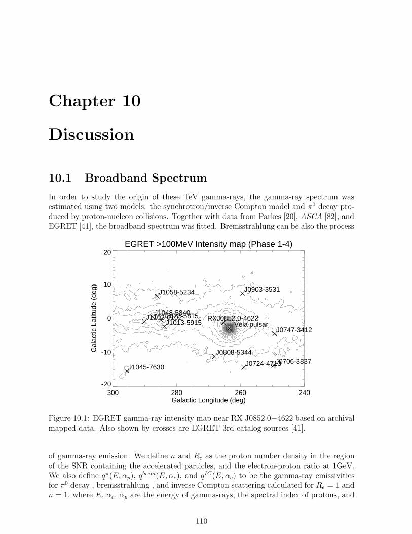
Chapter 10

Discussion

10.1 Broadband Spectrum

In order to study the origin of these TeV gamma-rays, the gamma-ray spectrum wasestimated using two models: the synchrotron/inverse Compton model and π0 decay pro-duced by proton-nucleon collisions. Together with data from Parkes [20], ASCA [82], andEGRET [41], the broadband spectrum was fitted. Bremsstrahlung can be also the process

EGRET >100MeV Intensity map (Phase 1-4)

-20

-10

0

10

20

Gal

actic

Lat

itude

(de

g)

300 280 260 240Galactic Longitude (deg)

RXJ0852.0-4622Vela pulsar

J0706-3837J0724-4713

J0747-3412

J0808-5344

J0903-3531

J1013-5915J1027-5815

J1045-7630

J1048-5840

J1058-5234

J1102-6102

Figure 10.1: EGRET gamma-ray intensity map near RX J0852.0−4622 based on archivalmapped data. Also shown by crosses are EGRET 3rd catalog sources [41].

of gamma-ray emission. We define n and Re as the proton number density in the regionof the SNR containing the accelerated particles, and the electron-proton ratio at 1GeV.We also define qπ(E, αp), qbrem(E,αe), and qIC(E, αe) to be the gamma-ray emissivitiesfor π0 decay , bremsstrahlung , and inverse Compton scattering calculated for Re = 1 andn = 1, where E, αe, αp are the energy of gamma-rays, the spectral index of protons, and

110

that of electrons, respectively. The gamma-ray flux is given as

Fγ(E) ∝ nqπ(E, αp) + nReqbrem(E,αe) + Req

IC(E, αe). (10.1)

The gamma-ray emissivities for the above three processes are shown in Figure 10.2 [31].From Figure 10.2, the ratio between the emissivity for bremsstrahlung and that for π0 de-

Figure 10.2: Gamma-ray emissivities for π0 decay (dot-dashed line) , bremsstrahlung(solid line) , and inverse Compton scattering for various radiation fields (the other lines).These emissivities were calculated by Gaisser, Protheroe and Stanev [31] assuming theelectron-proton ratio is unity, the number density of protons is 1cm−3, and the spectralindex of both protons and electrons is −2.

cay is of order 10 at around 1TeV. Re, however is of order 0.01. Therefore bremsstrahlungis not taken into consideration in this thesis.

10.1.1 Synchrotron/inverse Compton Model

The high-energy electrons emit photons both by synchrotron radiation process and inverseCompton scattering with the Cosmic Microwave Background (CMB). The former emitsradio and X-rays, and the latter TeV gamma-rays. In order to evaluate the spectrum oftheir emissions, the energy spectrum of the relativistic electrons is assumed to be

Q(Ee) = A

(Ee

mec2

)−α

exp

(− Ee

Emax

), (10.2)

where Ee, me, α, and Emax are the electron energy, the mass of the electron, the spectralindex, and the maximum accelerated energy of electrons, respectively. From the above

111

assumption, the differential flux is approximated as

dF (E)

dE=

1

4πd2· V Q(Ee)dEe · 1

τ· 1

dE=

V

4πd2Q(Ee)

dEe

dE

1

τ, (10.3)

where V , d, and τ are the volume of the emission region, the distance from the earth, andthe average time that one electron with the energy of Ee emit the energy E. Ee is givenas

Ee = γemec2, (10.4)

where γe is the Lorentz factor of the electron. Here we used δ-function approximation[79] [68]. In case of inverse Compton process, E is given as

E = γ2e ECMB, (10.5)

because γehν ¿ mec2, where ECMB is the average energy of the CMB. τ is approximated

as1

τIC

∼ 1

E

[dEe

dt

]

IC

=1

E

4

3σT cγ2

eUCMB =4

3

σT cUCMB

ECMB

, (10.6)

where the σT and UCMB are the cross section of Thomson scattering and the energydensity of CMB, respectively. From Equations (10.2), (10.3), (10.4), (10.5), and (10.6),the differential flux of gamma-rays from inverse Compton process is given as

[dF (E)

dE

]

IC

=V

4πd2

2

3

A

mec2σT cUCMB

(ECMB

mec2

)α−32

(E

mec2

)−α+12

exp

[−mec

2

Emax

(E

ECMB

) 12

].

(10.7)From Equation (10.7), the power-law index of the gamma-ray spectrum should be 1.5 ifthe α is 2 which is predicted by the diffusive shock acceleration discussed in Section 2.3.

In the case of the synchrotron radiation, in order to obtain the differential flux, theUCMB can be replaced with

UB =B2

8π, (10.8)

where B and UB are the ambient magnetic field and its energy density, respectively. ECMB

can be also replaced with

Esync = 0.29hνcπ

4, (10.9)

where the Esync is the peak energy of the synchrotron radiation (again δ-function approx-imation). After these replacements, the differential flux is given as

[dF (E)

dE

]

sync

=Vsync

4πd2

2

3

A

mec2σT cUB

(Esync

mec2

)α−32

(E

mec2

)−α+12

exp

[−mec

2

Emax

(E

Esync

) 12

].

(10.10)The power-law index of the synchrotron spectrum becomes equal to that of Equation(10.7).

In these calculations, there are four parameters, the power-law index of the electronspectrum, the maximum accelerated energy of the electrons, the magnetic field, and thescale factor V A/4πd2. In order to fit this model, the radio data obtained at Parkesobservatory [20], X-ray data from ASCA satellite [82], EGRET diffuse emission [41], and

112

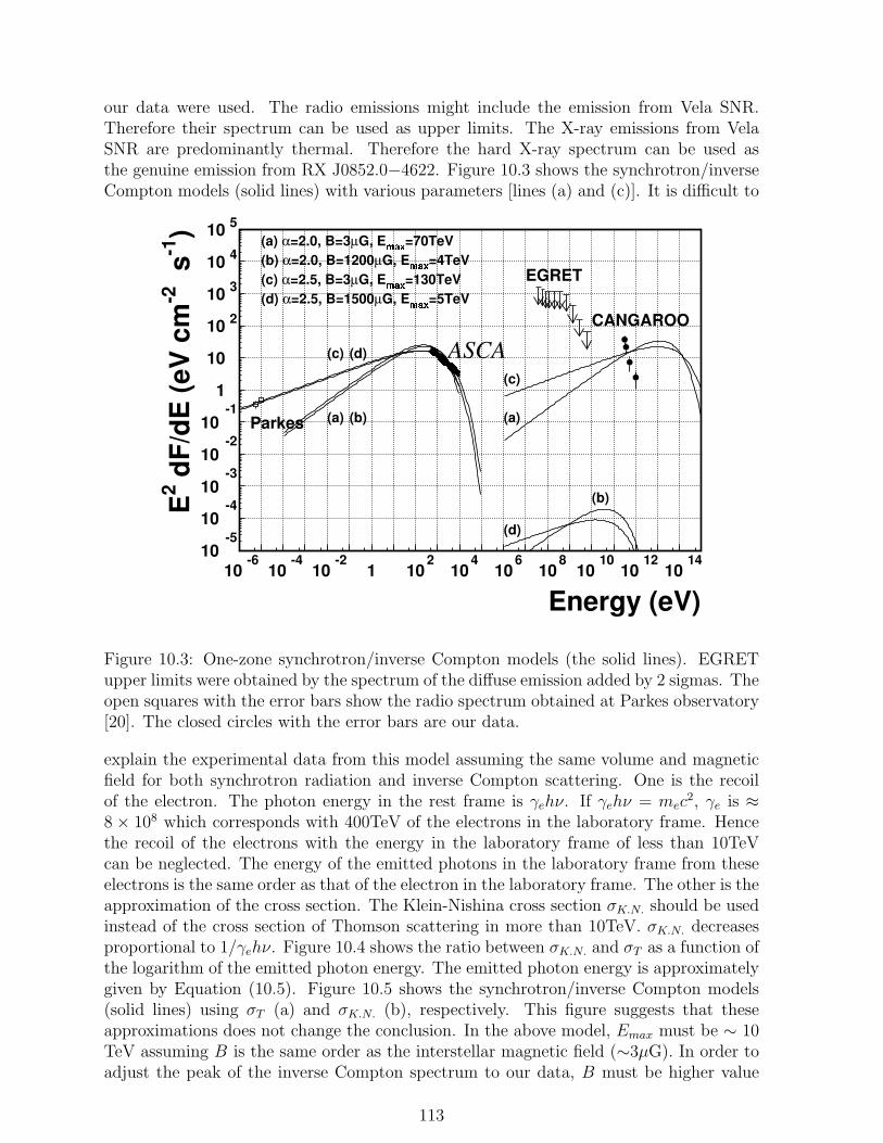
our data were used. The radio emissions might include the emission from Vela SNR.Therefore their spectrum can be used as upper limits. The X-ray emissions from VelaSNR are predominantly thermal. Therefore the hard X-ray spectrum can be used asthe genuine emission from RX J0852.0−4622. Figure 10.3 shows the synchrotron/inverseCompton models (solid lines) with various parameters [lines (a) and (c)]. It is difficult to

Figure 10.3: One-zone synchrotron/inverse Compton models (the solid lines). EGRETupper limits were obtained by the spectrum of the diffuse emission added by 2 sigmas. Theopen squares with the error bars show the radio spectrum obtained at Parkes observatory[20]. The closed circles with the error bars are our data.

explain the experimental data from this model assuming the same volume and magneticfield for both synchrotron radiation and inverse Compton scattering. One is the recoilof the electron. The photon energy in the rest frame is γehν. If γehν = mec

2, γe is ≈8 × 108 which corresponds with 400TeV of the electrons in the laboratory frame. Hencethe recoil of the electrons with the energy in the laboratory frame of less than 10TeVcan be neglected. The energy of the emitted photons in the laboratory frame from theseelectrons is the same order as that of the electron in the laboratory frame. The other is theapproximation of the cross section. The Klein-Nishina cross section σK.N. should be usedinstead of the cross section of Thomson scattering in more than 10TeV. σK.N. decreasesproportional to 1/γehν. Figure 10.4 shows the ratio between σK.N. and σT as a function ofthe logarithm of the emitted photon energy. The emitted photon energy is approximatelygiven by Equation (10.5). Figure 10.5 shows the synchrotron/inverse Compton models(solid lines) using σT (a) and σK.N. (b), respectively. This figure suggests that theseapproximations does not change the conclusion. In the above model, Emax must be ∼ 10TeV assuming B is the same order as the interstellar magnetic field (∼3µG). In order toadjust the peak of the inverse Compton spectrum to our data, B must be higher value

113

fic2

0

0.25

0.5

0.75

1

11 12 13 14Log10E(eV)

σ K.N

./σT

Figure 10.4: Ratio between the Klein-Nishina cross section and the cross section of Thom-son scattering as a function of the logarithm of the emitted photon energy. The emittedphoton energy is approximately given by Equation (10.5).

Figure 10.5: Synchrotron/inverse Compton models (solid lines): cross section of theThomson scattering (a), Klein-Nishina cross section (b). The power-law index of theelectron spectrum, the maximum accelerated energy of the electrons, the magnetic fieldare assumed to be -2.5, 130TeV, and 3µG, respectively.

114

such as mG, and Emax must be lower value. However, these values lead to the very lowflux in TeV [lines (b) and (d) in Figure 10.3].

In order to avoid this difficulty, the different sizes of the emission regions in X-raysand TeV gamma-rays can be introduced [1], [73]. Because the angular resolution in TeVmeasurement is poor, the more extended emission for TeV gamma-rays than that of X-rayscan be allowed. The ratio VTeV /VX of the emission volumes in each energy region is addedto the previous model as a new parameter. Figure 10.6 shows the synchrotron/inverseCompton model with the different sizes of the emission regions in X-rays and TeV gamma-rays (two-zone model). VTeV /VXs are fitted to 2.5 × 105 for (a), and 7 × 105 for (b) in

Figure 10.6: Synchrotron/inverse Compton models with the different sizes of the emissionregions in X-rays and TeV gamma-rays (two-zone model) [1], [73]. VTeV /VXs are 2.5×105

for (a) and 7× 105 for (b), respectively.

Figure 10.6, respectively. The instrumental upper limit of the VTeV /VX can be estimatedusing VTeV /VX ≈ (dθTeV )3/(dθX)3 = θ3

TeV /θ3X . Since the TeV emission size was estimated

to be ≈ 0.10 in Chapter 7 with the large uncertainty, θTeV should be around the size ofthe PSF of CANGAROO. X-ray data indicate extended emission. Figure 10.7 shows theX-ray image of ASCA GIS based on the archival data. The sizes of the 65% contour ofASCA data are approximately 0.116 along the major axis and 0.060 along the minoraxis, respectively. Using these values, θX is ≈ 0.083. From these consideration, the upperlimit is given as

[VTeV

VX

]

max

≈[(

θTeV

θX

)3]

max

=

(0.24

0.083

)3

≈ 24 ¿ (2.5− 7)× 105. (10.11)

Equation 10.11 indicates that this simple two-zone model is highly unlikely to explainthe broadband spectrum. More complicated situation can be considered. Figure 10.8

115

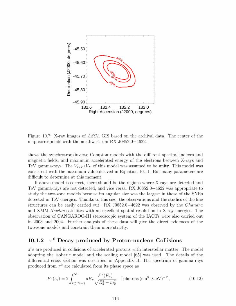
132.6 132.4 132.2 132.0Right Ascension (J2000, degrees)

-45.90

-45.80

-45.70

-45.60

-45.50

Dec

linat

ion

(J20

00, d

egre

es)

40%

40%

65%

80%

Figure 10.7: X-ray images of ASCA GIS based on the archival data. The center of themap corresponds with the northwest rim RX J0852.0−4622.

shows the synchrotron/inverse Compton models with the different spectral indexes andmagnetic fields, and maximum accelerated energy of the electrons between X-rays andTeV gamma-rays. The VTeV /VX of this model was assumed to be unity. This model wasconsistent with the maximum value derived in Equation 10.11. But many parameters aredifficult to determine at this moment.

If above model is correct, there should be the regions where X-rays are detected andTeV gamma-rays are not detected, and vice versa. RX J0852.0−4622 was appropriate tostudy the two-zone models because its angular size was the largest in those of the SNRsdetected in TeV energies. Thanks to this size, the observations and the studies of the finestructures can be easily carried out. RX J0852.0−4622 was observed by the Chandraand XMM-Newton satellites with an excellent spatial resolution in X-ray energies. Theobservation of CANGAROO-III stereoscopic system of the IACTs were also carried outin 2003 and 2004. Further analysis of these data will give the direct evidences of thetwo-zone models and constrain them more strictly.

10.1.2 π0 Decay produced by Proton-nucleon Collisions

π0s are produced in collisions of accelerated protons with interstellar matter. The modeladopting the isobaric model and the scaling model [65] was used. The details of thedifferential cross section was described in Appendix B. The spectrum of gamma-raysproduced from π0 are calculated from its phase space as

F γ(εγ) = 2

∫ ∞

Eminπ (εγ)

dEπF π(Eπ)√E2

π −m2π

[ photons (cm3 s GeV)−1], (10.12)

116

Figure 10.8: Synchrotron/inverse Compton models with the different spectral indexes −αand magnetic fields B, and maximum accelerated energy of the electrons Emax betweenX-rays and TeV gamma-rays. The ratio of the emission sizes between X-rays and TeVgamma-rays was assumed to be unity.

117

where Eπ is the π0 energy in GeV, mπ is its rest mass in GeV c−2, Fπ(Eπ) denotes the π0

spectrum, εγ is the is the gamma-ray energy in GeV, and Eminπ (εγ) is the minimum energy

of π0s to create photons of energy εγ, respectively. This is derived kinetically using thefollowing relation:

Eminπ (εγ) = εγ +

mπ2

4εγ

. (10.13)

The π0 spectrum, therefore, is written as

F π(Eπ) = 4πn0

∫ Emaxp

Eminp (Eπ)

dEpjp(Ep)dσπ(Eπ, Ep)

dEπ

[ pions (cm3 s GeV)−1], (10.14)

where n0 is the number density of protons where the interactions occur , Ep is the energyof cosmic ray protons in GeV, Emin

p (Eπ) is the minimum cosmic ray proton energy toproduce π0s of energy Eπ in GeV, and jp is the energy spectrum of cosmic ray protons,respectively. Here we assume

jp(Ep) =K

V

(E0

1050erg

)E−α

p exp

(− Ep

Emaxp

)[ protons (cm2 s GeV sr)−1], (10.15)

where V is the volume of the SNR shell, E0 is the total energy of cosmic ray protons in theobserved part of the SNR, and Emax

p is the maximum accelerated energy of protons. Theassumption of the exponential cut off is adopted because it fits better to the experimentaldata [31]. K is the normalization factor which satisfy

∫ ∞

mpc2

4π

cjp(Ep)EpdEp =

E0

V. (10.16)

Finally dσπ(Eπ, Ep)/dEπ is the differential cross section.From Equation (10.12), the differential flux on the earth can be calculated from

fγ(εγ) =V

4πd2F γ(εγ) [ photons (cm2 s GeV)−1], (10.17)

where d is the distance of the SNR from the earth. However, Equation (10.15) contains V .The V in Equation (10.17) is canceled out. This model has three parameters, the powerlaw index of protons α, the maximum accelerated energy of protons Emax

p , and the scalefactor A ≡ (E0/1050erg)(n0/protons cm−3)(d/0.5kpc)−2. The integral in Equation (10.12)can be calculated independently when the Ep and εγ are fixed. Using the tables obtainedfrom this calculation, the gamma-ray flux can be estimated together with the assumedproton spectrum. Above MeV energies, the diffuse data of the EGRET and CANGAROOdata are available. The goodness of the fits with this model was investigated. Figure10.9 shows the allowed region determined from the χ2/DOF values for various A andEp

max. Here α was assumed to be 2.0 predicted by the diffusive shock acceleration theoryassuming the strong shock wave as was discussed in Section 2.3. The contours show thedifference in χ2/DOF from the minimum value, 1σ, 2σ, 3σ, and 4σ, respectively. Thebest fit point showed the χ2/DOF of 0.53 with the best fitted values of Emax

p = 2.4TeVand A =1.6. Figure 10.10 shows the SED estimated from the best fit model (the solidline). In order to verify the assumption of the spectral index, the spectra were alsocalculated for the index of −2.2, 2.4, and 1.8. Figure 10.11 shows the SED of the various

118

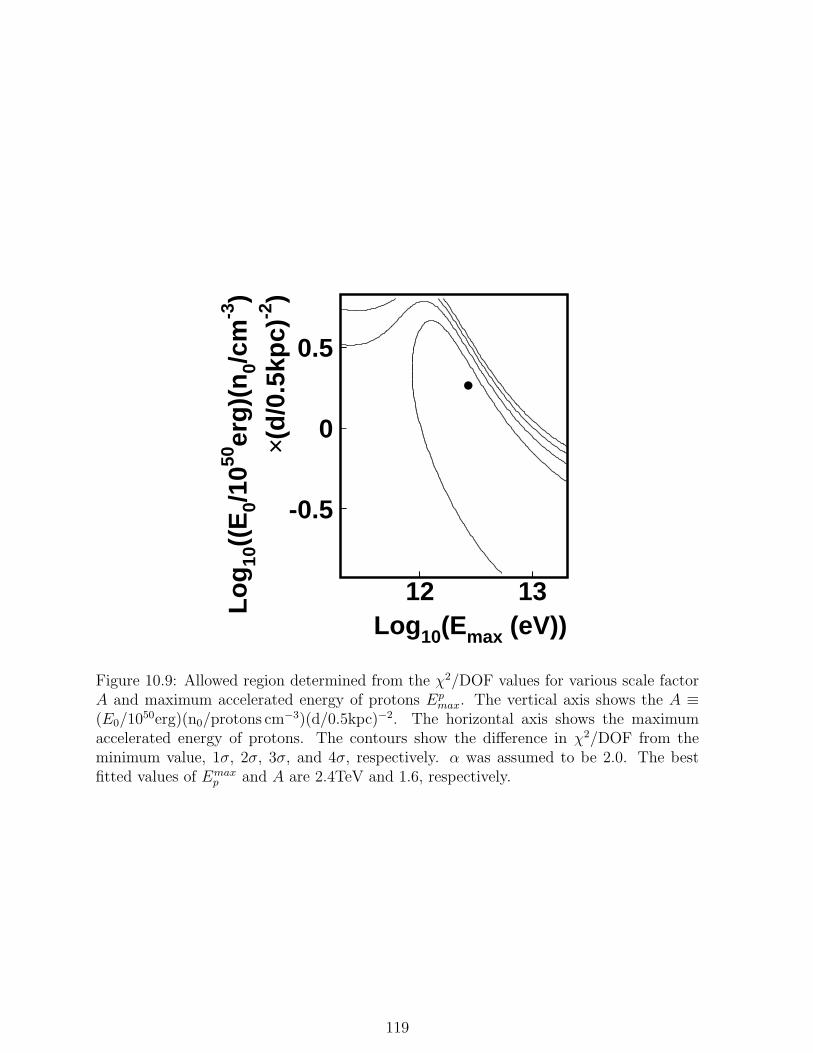
-0.5

0

0.5

12 13

emax vs a

Log10(Emax (eV))

Lo

g10

((E

0/10

50er

g)(

n0/

cm-3

)×(

d/0

.5kp

c)-2

)

•

Figure 10.9: Allowed region determined from the χ2/DOF values for various scale factorA and maximum accelerated energy of protons Ep

max. The vertical axis shows the A ≡(E0/1050erg)(n0/protons cm−3)(d/0.5kpc)−2. The horizontal axis shows the maximumaccelerated energy of protons. The contours show the difference in χ2/DOF from theminimum value, 1σ, 2σ, 3σ, and 4σ, respectively. α was assumed to be 2.0. The bestfitted values of Emax

p and A are 2.4TeV and 1.6, respectively.

119

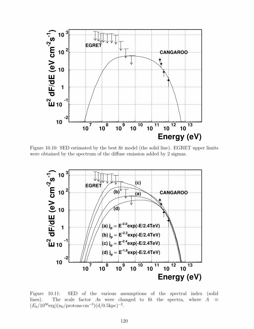
Figure 10.10: SED estimated by the best fit model (the solid line). EGRET upper limitswere obtained by the spectrum of the diffuse emission added by 2 sigmas.

Figure 10.11: SED of the various assumptions of the spectral index (solidlines). The scale factor As were changed to fit the spectra, where A ≡(E0/1050erg)(n0/protons cm−3)(d/0.5kpc)−2.

120

assumptions of the spectral index. The softer spectrum of the protons than the best fitmodel were highly unlikely. The harder spectra which were expected from the non-linearacceleration scheme [11] were also favored. Figure 10.12 shows the differential spectrumestimated by the best fit model (the solid line). In case of SNR RX J1713.7−3946,

Figure 10.12: Differential spectrum estimated by the best fit model (the solid line).EGRET upper limits were obtained by the spectrum of the diffuse emission added by2 sigmas.

(E0/1050erg)(n0/protons cm−3)(d/1kpc)−2 was 8 from the CANGAROO data [25]. Theestimation of the distance by NANTEN data was 1kpc [29]. They estimated the E0 to be1048 erg [29]. The volume of the observed region was not considered in the parameter A.In case of RX J0852.0−4622, the A including this consideration is given as

A ≡ 1

Ω

(E0

1050erg

)(n0

protons cm−3

)(d

0.5kpc

)−2

, (10.18)

where Ω is the solid angle of the observed volume. Ω is 0.033 shown in Figure 7.9. Atotal cosmic-ray energy of E0/Ω = 1048 to 1050 erg is required when n0 = 5000 to 50protons cm−3 assuming d = 0.5kpc . These are consistent with the typical density of themolecular clouds. Further observation of this region by NANTEN is interesting.

10.2 Summary of Discussions

Our data strongly favor TeV gamma-rays from π0 decay and low flux from synchrotron /inverse Compton under the simple one-zone model. A total cosmic-ray energy of E0/Ω =1048 to 1050 erg is required when n0 = 5000 to 50 protons cm−3 assuming d = 0.5kpc. Thetwo-zone model of synchrotron/inverse Compton model, however, can also explain the

121

SED if there are fine structures in the X-ray emissions. In order to determine the detailsof the model, further observations with better detectors are needed. The observations ofXMM-Newton and Chandra satellites have revealed the fine structures of the shock frontin SN1006 and RX J1713.7−3946. The results of analysis for XMM-Newton and Chandradata of this SNR are eagerly awaited. Further analysis with next generation IACTs,which have a better angular resolution, will reveal the environments of the accelerationand emission regions. NANTEN observations will give us the direct information about theambient matter density. If dense molecular clouds were found near there, it will stronglysupport hadronic origin of TeV gamma-rays in this SNR.

More SNRs which emit non-thermal X-ray should be further investigated by IACTs.RCW86 is one of them. It has been already observed by CANGAROO and the dataare under analysis. Next generation IACTs will detect these SNRs and establish thehypothesis that the Galactic cosmic rays are mainly accelerated by the SNRs.

122

Chapter 11

Conclusion

RX J0852.0−4622 (G266.2−1.2) was observed with the CANGAROO-II 10-m telescopein 2002 and 2003. The pointing direction was where ASCA detected non-thermal X-ray emissions (NW-rim). A total of ∼ 187 hours data was obtained. These data wereanalyzed using the imaging analysis with the likelihood method. The resulting α distri-bution indicated the excess events with the statistical significance of 6.4 σ. The ratioN(α < 15)/N(α < 30) suggested a marginally extended emission, but still consistentwith the point source within statistical errors. The significance map of the gamma-ray emission coincided with the X-ray maximum point. If we assume the extendedemission, its size is ≈ 0.10. The differential flux shows 0.25±0.06 Crab at 500GeVwith the spectral index of −4.5±0.7. The gamma-ray spectra were estimated using twomodels: the synchrotron/inverse Compton model and decay of π0s produced by proton-nucleon collisions. Our data strongly favored TeV gamma-rays from π0 decay and lowflux from synchrotron/inverse Compton for simple assumptions. A total cosmic-ray en-ergy of E0/Ω = 1048 to 1050 erg is required when molecular cloud density is 5000 to 50protons cm−3 assuming the distance is 0.5 kpc. The two-zone model of synchrotron/inverseCompton model, however, can also explain the spectrum using many parameters whichcan not be individually determined by observations. In order to constrain the models,further results with better detectors, such as XMM-Newton and Chandra, NANTEN,and next generation IACTs, are needed. The detection of more SNRs will establish thehypothesis that the Galactic cosmic rays are mainly accelerated by the SNRs.

123

Acknowledgement

I would like to thank my supervisor, Prof. Masaki Mori (Institute for Cosmic Ray Re-search, The University of Tokyo;ICRR) for his support over the past five years. I alsowish to thank Prof. Ryoji Enomoto (ICRR), Dr. Ken’ichi Tsuchiya (ICRR) for theirsuggestions in my research work.

I also wish to thanks my colleagues Dr. Akiko Kawachi (ICRR), Dr. Satoshi Hara(ICRR), Dr. Michiko Ohishi (ICRR), Dr. Shigeto Kabuki (ICRR), Dr. Ryoji Kurosaka(ICRR), Dr. Yuuki Adachi (ICRR), Dr. Ryuta Kiuchi (ICRR), for their support andencouragement.

I would like to thank Prof. Shohei Yanagita (Ibaraki University), Prof. Tsuguya Naito(Yamanashi Gakuin University), Prof. Tatsuo Yoshida (Ibaraki University), Dr. LeonidT. Ksenofontov (ICRR) for their theoretical support. I would like to thank Prof. ToruTanimori (Kyoto University) for his suggestion in my research work.

All other colleagues in the CANGAROO group are given my best thanks.

124

Bibliography

[1] Aharonian, F. A., Atoyan, A. M., Kifune, T., 1997, Mon. Not. R. Astron. Soc., 291,162

[2] Aharonian, F., et al., 2000, ApJ, 539, 317

[3] Aharonian, F., et al., 2001, A&A, 370, 112

[4] Alvarez, L., Compton, A., 1933, Phys. Rev., 43, 835

[5] Aschenbach, B., 1998, Nature, 396, 141

[6] Aschenbach, B., 1999, A&A, 350, 997

[7] Baade, W., Zwicky, F., 1934, Phys. Rev., 46, 76

[8] Bamba, A., Koyama, K., Tomida, H., 2000, PASJ, 52, 1157

[9] Baum, W. A., Dunkelman, L., 1955, J. Opt. Soc. Am., 45, 166

[10] Bell, A. R. , 1978, MNRAS, 182, 147

[11] Berezhko, E. G., Ksenofontov, L. T., Volk, 2002, A&A, 395, 943

[12] Blandford, R. D., Ostriker, J. P., 1978, ApJ, 221, L29

[13] Buckley, J. H., et al., 1998, A&A, 329, 639

[14] Burgess, C. P., Zuber, K., 2000, Astropart. Phys., 14, 1

[15] Butt, Y. M., 2002, Nature, 418, 499

[16] Cha, A. N., Sembach, K. R., Danks, A. C., 1999, ApJ, 515, L25

[17] Chen, W., Gehrels, N., 1999, ApJ, 514, L103

[18] Combi, J. A., Romero, G. E., Benaglia, P., 1999, ApJ, 519, L177

[19] Drury, L. O’C., Aharonian, F. A., Volk, H. J., 1994, A&A, 287, 959

[20] Duncan, A. R., Green, D. A., 2000, A&A, 364, 732

[21] Ellison, D. C., Slane, P., Gaensler, B. M., 2001, ApJ, 563, 191

[22] Enomoto R., 2000, DST10 module’s manual

125

[23] Enomoto, R., Tanimori, T., Asahara, A., et al., 2001, Proc. 27th ICRC (Hamburg)6, 2477

[24] Enomoto, R., Hara, S., Asahara, A., et al., 2002, Astropart. Phys., 16, 235

[25] Enomoto, R., Tanimori, T., Naito, T., et al., 2002, Nature, 416, 823

[26] Esposito, J. A., et al., 1996, ApJ, 461, 820

[27] Fermi, E. , Phys. Rev., 75, 1169

[28] Frank, I. M., Tamm, Ig., 1937, Dolk. Akad. Nauk., SSSR, 14 (3), 109

[29] Fukui, Y., et al., PASJ, 2003, 55, L61

[30] Gaisser, T. K., 1990, Cosmic Rays and Particle Physics (Cambridge Univ. Press)

[31] Gaisser, T. K., Protheroe, R. J., Stanev, T., 1998, A&A, 492, 219

[32] Galbraith, W., Jelly, J. V., 1953, Nature, Lond., 171, 349

[33] GEANT, CERN Program Library Long Writeup W5013

[34] Ginzburg, V. L., 1953, Dokl. Akad. Nauk. SSSR, 92, 1133

[35] Ginzburg, V. L., Syrovatskii, S., 1965, Ann. Rev. Astron. Astrophys., 3, 297

[36] Gorres, J., et al., 1998, Phys. Rev. Lett., 80, 2554

[37] Gupta, M., Webber, W. R., 1989, 340, 1124

[38] Hall, T. A., et al., 2003, ApJ, 583, 853

[39] Hara, T., Kifune, T., Matsubara, Y., et al., 1993, Nucl. Instr. Meth. A, 332, 300

[40] Hartman, R. C., et al., 1979, ApJ, 230, 597

[41] Hartman, R. C., 1999, ApJS, 123, 79

[42] Hayakawa, S., 1952, Prog. Theo. Phys., 8, 571

[43] Hayakawa, S., 1956, Prog. Theo. Phys., 15, 233

[44] Hayashida, N., et al., 1994, Phys. Rev. Lett., 73, 3491

[45] Heitler, W., 1956, Quantum Theorie of the Radiation (Oxford)

[46] Hillas, A. M., 1982, J. Phys. G8, 1475

[47] Itoh, C., et al., 2002, A&A, 396, L1

[48] Itoh, C., et al., 2003, A&A, 402, 443

[49] Iyudin, A. F., et al., 1998, Nature, 396, 142

[50] Jelly, J. V., 1958, Cherenkov Radiation and its Application (Pergamon Press), 219

126

[51] Kabuki, S., et al., 2003, Nucl. Instr. Meth. A500, 318

[52] Kawachi, A., Hayami, Y., Jimbo, J., et al., 2001, Astropart. Phys., 14, 261

[53] Kerrick, A. D., et al., 1995, ApJ, 438, L59

[54] Kifune, T., Tanimori, T., Ogio, S., et al., 1995, ApJ, 438, L91

[55] Koyama, K., et al., 1995, Nature, 378, 255

[56] Koyama, K., et al., 1997, PASJ, 49, L7

[57] Li, T., Ma, Y., 1972, ApJ, 272, 317

[58] May, J., Murphy, D. C., Thaddeus, P., 1988, A&AS, 73, 51

[59] Mereghetti, S., 2001, ApJ, 548, L213

[60] Mohanty, G., Biller, S., Carter-Lewis, D. A., et al., 1998, Astropart. Phys., 9, 15

[61] Moriguchi, Y., et al., 2001, PASJ, 53, 1025

[62] Morison, P., 1958, Nuovo Cimento, 7, 858

[63] Muraishi, H., et al., 2000, A&A, 354, L57

[64] Muraishi, H., Tanimori, T., Yanagita, S., et al., 1998, A&A, 354, L57

[65] Naito T., Takahara F., 1994, J. Phys. G: Nucl. Part. Phys. 20, 477

[66] Nomachi, M., et al., 1994, Proc. Int. Conf. on Computing on High Energy Physics’94, LBL-35822, 114

[67] Norman, E. B., et al., 1998, Phys. Rev. C., 57, 2010

[68] eds. Oda, M., Nishimura, J., Sakurai, K., 1983, Uchusen-Butsurigaku, AsakuraShoten (in Japanese)

[69] Ohishi, M., Mori, M., 2001, CANGAROO internal report

[70] Okumura K., 2000, CALIB7 (CALIB10) module’s manual

[71] Okumura, K., et al., 2002, ApJ, 579, L9

[72] Ozaki, M., 1998, ph. D thesis

[73] Pannuti, T. G., et al., 2003, ApJ, 593, 377

[74] Pavlov, G. G., et al., 2001, ApJ, 559, L131

[75] Punch, M., et al., 1991, Proc. 22th ICRC (Dublin) 1, 464

[76] Punch, et al., 1992, Nature, 358, 477

[77] Reimer, O., Pohl, M., 2002, A&A, 390, L43

127

[78] Reynolds, S. P., Ellison, D. C., 1992, ApJ, 399, L75

[79] Rybicki, G. B., Lightman, A. P., 1979, Radiative processes in astrophysics (A Wiley-Interscience publication)

[80] eds. Sekido, Y., Elliot, H., 1985, Early history of cosmic ray studies (D. ReidelPublishing Company)

[81] Simpson, J. A., 1983, Ann. ReV. Nucl. Part. Sci., 33, 323

[82] Slane, P., et al., 2001, ApJ, 548, 814

[83] Sturner, S. J., et al., 1997, 490, 619

[84] Swanenburg, B. N., et al., 1981, 243, L69

[85] Tanimori, T., et al., 2001, Proc. 27th ICRC (Hamburg), 6, 2465

[86] Tanimori, T., Hayami, Y., Kamei, S., et al., 1998, 497, L25

[87] Tanimori, T., Sakurazawa, K., Dazeley, S. A., et al., 1998, ApJ, 492, L33

[88] Tsunemi, et al., 2000, PASJ, 52, 887

[89] Vink, J., Laming, J. M., ApJ, 584, 758

[90] Wdowczyk, J. and Wolfendale, A. W., 1989, Ann. ReV. Nucl. Part. Sci., 39, 43

[91] Weekes, T. C., et al., 1989, ApJ, 342, 379

[92] Weekes, T. C.,1988, Phys. Rep., 160, 1

[93] Willingale, R., et al., 1996, Mon. Not. R. Astron. Soc., 278, 749

[94] http://owl.gsfc.nasa.gov/intro.html

128

Appendix A

Definitions of the Image Parameters

We define the index of each pixel, the center of each pixel, and the amount of photons ineach pixel as i, (xi, yi), and si, respectively. The averages are defined as follows:

〈x〉 =

∑sixi∑si

, (A.1)

〈x2〉 =

∑six

2i∑

si

, (A.2)

〈x3〉 =

∑six

3i∑

si

, (A.3)

〈y〉 =

∑siyi∑si

, (A.4)

〈y2〉 =

∑siy

2i∑

si

, (A.5)

〈y3〉 =

∑siy

3i∑

si

, (A.6)

〈xy〉 =

∑sixiyi∑

si

, (A.7)

〈x2y〉 =

∑six

2i yi∑

si

, (A.8)

〈xy2〉 =

∑sixiy

2i∑

si

. (A.9)

The coordinate (〈x〉, 〈y〉) correspond to the centroid of the image. The following is furtherdefinitions:

σx2 = 〈x2〉 − 〈x〉2, (A.10)

σy2 = 〈y2〉 − 〈y〉2, (A.11)

σxy = 〈xy〉 − 〈x〉〈y〉, (A.12)

σx3 = 〈x3〉 − 3〈x2〉〈x〉+ 2〈x〉3, (A.13)

σy3 = 〈y3〉 − 3〈y2〉〈y〉+ 2〈y〉3, (A.14)

σx2y = 〈x2y〉 − 2〈xy〉〈x〉+ 2〈x〉2〈y〉 − 〈x2〉〈y〉, (A.15)

σxy2 = 〈xy2〉 − 2〈xy〉〈y〉+ 2〈y〉2〈x〉 − 〈y2〉〈x〉. (A.16)

129

Here we introduce d = σy2 − σx2 and z = (d2 + 4σxy)1/2. Length and Width are defined

as follows:

Width =

(σx2 + σy2 − z

2

)1/2

, (A.17)

Length =

(σx2 + σy2 + z

2

)1/2

. (A.18)

If an assumed source position in the field of view is (xs, ys) and the Distance vector ~D= (xD, yD) is defined as

~D = (xs − 〈x〉, ys − 〈y〉), (A.19)

thenDistance = (x2

D + y2D)1/2. (A.20)

If an unit vector of the major axis, ~u = (xu, yu), is

~u =

((z − d

2z

)1/2

, sign(σxy)

(z + d

2z

)1/2)

, (A.21)

then

α = cos−1

(xuxD + yuyD

Distance

). (A.22)

The Asymmetry vector ~A is~A = −σA~u, (A.23)

where

σA = (σx3 cos3 φ + 3σx2y cos2 φ sin φ + 3σxy2 cos φ sin2 φ + σy3 sin3 φ)1/3 (A.24)

and φ is the angle of ~u with respect to the x axis. Asymmetry is defined as

Asymmetry = sign( ~A · ~D)|σA|

Length=

~A · ~D

Distance Length cos α. (A.25)

130

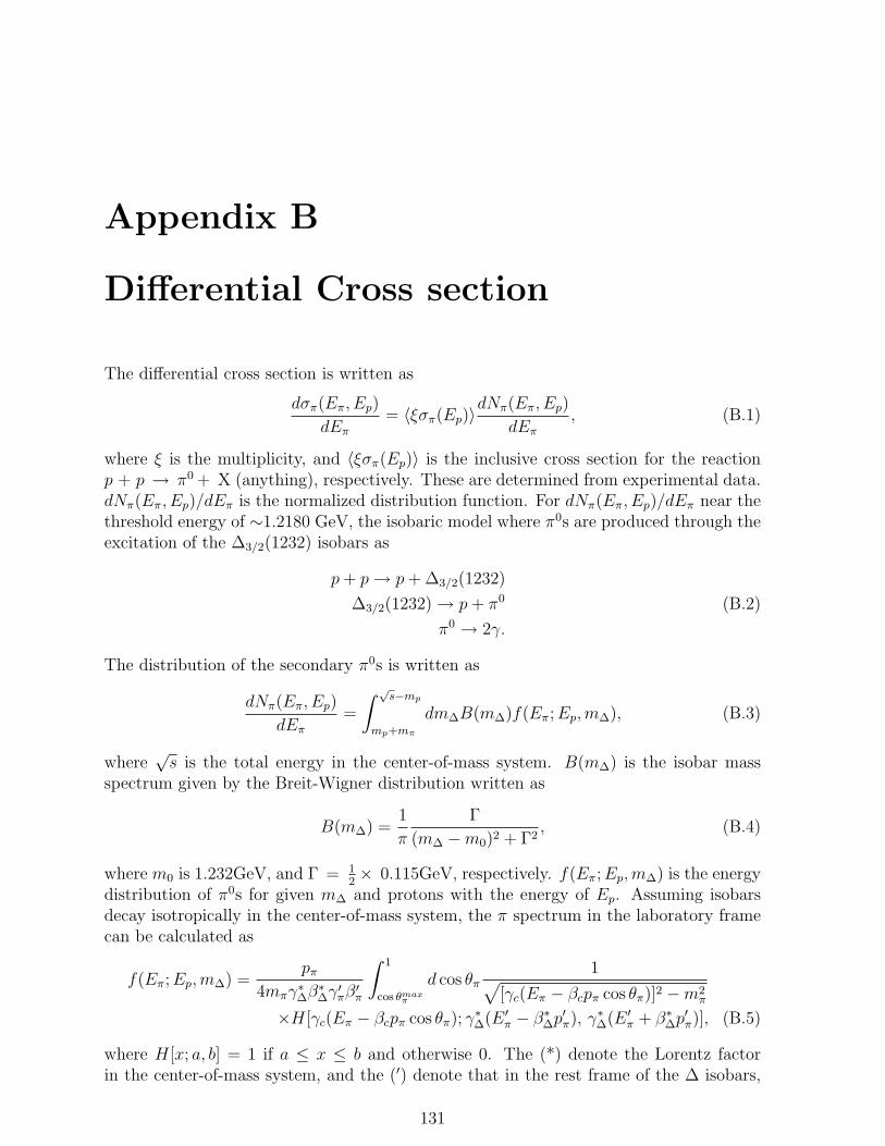
Appendix B

Differential Cross section

The differential cross section is written as

dσπ(Eπ, Ep)

dEπ

= 〈ξσπ(Ep)〉dNπ(Eπ, Ep)

dEπ

, (B.1)

where ξ is the multiplicity, and 〈ξσπ(Ep)〉 is the inclusive cross section for the reactionp + p → π0 + X (anything), respectively. These are determined from experimental data.dNπ(Eπ, Ep)/dEπ is the normalized distribution function. For dNπ(Eπ, Ep)/dEπ near thethreshold energy of ∼1.2180 GeV, the isobaric model where π0s are produced through theexcitation of the ∆3/2(1232) isobars as

p + p → p + ∆3/2(1232)

∆3/2(1232) → p + π0 (B.2)

π0 → 2γ.

The distribution of the secondary π0s is written as

dNπ(Eπ, Ep)

dEπ

=

∫ √s−mp

mp+mπ

dm∆B(m∆)f(Eπ; Ep,m∆), (B.3)

where√

s is the total energy in the center-of-mass system. B(m∆) is the isobar massspectrum given by the Breit-Wigner distribution written as

B(m∆) =1

π

Γ

(m∆ −m0)2 + Γ2, (B.4)

where m0 is 1.232GeV, and Γ = 12× 0.115GeV, respectively. f(Eπ; Ep,m∆) is the energy

distribution of π0s for given m∆ and protons with the energy of Ep. Assuming isobarsdecay isotropically in the center-of-mass system, the π spectrum in the laboratory framecan be calculated as

f(Eπ; Ep,m∆) =pπ

4mπγ∗∆β∗∆γ′πβ′π

∫ 1

cos θmaxπ

d cos θπ1√

[γc(Eπ − βcpπ cos θπ)]2 −m2π

×H[γc(Eπ − βcpπ cos θπ); γ∗∆(E ′π − β∗∆p′π), γ∗∆(E ′

π + β∗∆p′π)], (B.5)

where H[x; a, b] = 1 if a ≤ x ≤ b and otherwise 0. The (*) denote the Lorentz factorin the center-of-mass system, and the (′) denote that in the rest frame of the ∆ isobars,

131

and Cs denote the Lorentz factor of center-of-mass system with respect to the laboratoryframe.

For higher energies, the scaling model was used. Using the Lorentz invariant crosssection, the distribution of the secondary π0s in the laboratory frame is written by

dNπ(Eπ, Ep)

dEπ

=2π

√E2

π −m2π

〈ξσπ(Ep)〉∫ 1

cos θmaxπ

d cos θπ

(E∗

π

d3σ∗πd3p∗π

). (B.6)

The invariant cross section is determined from experimental data of π0 production.

132