Embed Size (px)
Citation preview

DOCTORAL THESIS
High precision applications of lattice gauge theoriesin the quest for new physics
Andrea Bussone
arX
iv:1
710.
0117
7v1
[he
p-la
t] 3
Oct
201
7

High precision applications of lattice gauge theoriesin the quest for new physics
CANDIDATE: Andrea BussoneSUPERVISOR: Michele Della MorteCO-SUPERVISOR: Claudio Pica
Dissertation for the degree of Doctor of Philosophy
CP3-OriginsDepartment of Mathematics and Computer Science
Submitted to the University of Southern Denmark
Corrected version:Tuesday 3rd October, 2017

Abstract
We present some aspects of high precision calculations in the context of Lattice Quantum FieldTheory. This work is a collection of three studies done during my Ph.D. period.
First we present how to use the reweighting technique to compensate for the breaking of unitaritydue to the use of different boundary conditions in the valence and sea sector. In particular whentwisted boundary conditions are employed, with θ twisting angle. In large volume we found thatthe breaking is negligible, while in rather small volumes an effect is present. The quark massappears to change with θ as a cutoff effect.
In the second part of the dissertation we present an optimization method for Hybrid Monte Carloperformances. The presented strategy is quite general and can be applied to Beyond StandardModel strongly interacting theories, for which the need for precision is becoming urgent nowadays.The work is based on the existence of a shadow Hamiltonian, an exactly conserved quantity alongthe Molecular Dynamics trajectory. The optimization method is economic since it only requiresthe forces to be measured, which are already used for the evolution from one configuration to thenew one. We found predictions for the cost of the simulations with an accuracy of 10% and wecould estimate the optimal parameters for the Omelyan integrator with mass-preconditioning andmulti time-scale.
In the last part of the work we address the calculation of electromagnetic corrections to the hadroniccontribution to the (g− 2) anomaly of the muon. A long standing discrepancy between theoreticalcalculations and experimental results is present. Each new Beyond Standard Model theory aimsat solving the discrepancy with the introduction of New Physics. But before invoking New Physicswe need to clear the sight from possible effects within the Standard Model. Firstly we discussdifferent implementations of QED on the lattice with periodic boundary conditions. Then weconsider applications of that for the muon anomaly. In this exploratory study we carefully matchedthe masses of the charged pions in the theory with and without QED. In that way we are able toaccess directly the electromagnetic corrections to the anomaly with smaller statistical errors. Wefound a visible effect at the percent level although consistent with zero within two sigmas.
Sammenfatning
Vi præsenterer nogle vigtige aspekter af højpræcisionsberegninger i forbindelse med lattice kvan-tefeltteori. Denne afhandling er en samling af tre studier udført i løbet af min Ph.d.-uddannelse.
Først præsenterer vi, hvordan man bruger reweighting-teknikken til at kompensere for unitæritets-bruddet forårsaget af brugen af forskellige randbetingelser i valens- og sea-sektoren. I særdeleshednår der anvendes twistede-randbet ingelse med twist-vinkel θ. I store volumener fandt vi, at brud-det er ubetydeligt, mens der for små volumener findes en effekt. Kvarkmassen ser ud til at ændresig med vinklen θ som en såkaldt cut-of-effekt.
I anden del af afhandlingen præsenterer vi en optimeringsmetode til at forbedre ydelsen af HybridMonte Carlo-algoritmen. Den fremstillede strategi er generel og kan anvendes til stærkt vek-selvirkende teorier udover standardmodellen for hvilke behovet for præcision er begyndt at blivenødvendigt. Strategien er baseret på eksistensen af en shadow Hamiltonian, en eksakt bevaret stør-relse langs Molecular Dynamics-banen. Optimeringsmetoden er økonomisk, da den kun kræver,at kræfterne måles, og disse er allerede nødvendige for udviklingen fra en konfiguration til dennæste. Vi fandt forudsigelser for omkostningerne ved simuleringerne med en nøjagtighed på 10 %,og vi kunne estimere de optimale parametre for Omelyan-integratoren med mass-preconditioningog multi time-scale.
Den sidste del af afhandlingen omhandler beregningen af de elektromagnetiske korrektioner tilden hadroniske del af (g − 2)-anomalien for myonen. For denne observable størrelse eksistererder en langvarig uoverensstemmelse mellem de teoretiske beregninger og de eksperimentelle resul-tater. Enhver ny teori udover stardardmodellen stiler efter at løse denne uoverensstemmelse ved atintroducere ny fysik, men før vi tyer til ny fysik, skal vi sikre os imod effekter genereret af standard-modellen selv. For det første diskuterer vi forskellige implementeringer af QED på gitteret medperiodiske randbetingelser. Derefter betragter anvendelsen af disse for myon-anomalien. I detteeksplorative studie, matchede vi nøje masserne af de ladede pioner både i teorien med og udenQED. På denne måde har vi mulighed for direkte at få adgang til de elektromagnetiske korrektionertil anomalien med mindre statistiske usikkerheder. Vi fandt en synlig effekt på procentniveauetselvom resultatet er i overensstemmelse med nul inden for to standardafvigelser.

Publications
This dissertation is based on the following published articles done at CP3-Origins during the threeyears of my Ph.D. studies:
article A. Bussone, M. Della Morte, M. Hansen and C. Pica, “On reweighting for twisted boundaryconditions,” Comput. Phys. Commun. (2017) doi:10.1016/j.cpc.2017.05.011 [arXiv:1609.00210[hep-lat]]. (Bussone et al., 2017)
conf. proc. A. Bussone, M. Della Morte, M. Hansen and C. Pica, “Reweighting twisted boundary condi-tions,” PoS LATTICE 2015 (2016) 021 [arXiv:1509.04540 [hep-lat]]. (Bussone et al., 2016b)
conf. proc. A. Bussone, M. Della Morte, V. Drach, M. Hansen, A. Hietanen, J. Rantaharju andC. Pica, “A simple method to optimize HMC performance,” PoS LATTICE 2016 (2016)260 [arXiv:1610.02860 [hep-lat]]. (Bussone et al., 2016a)
conf. proc. A. Bussone, M. Della Morte and T. Janowski, “Electromagnetic corrections to the hadronicvacuum polarization of the photon within QEDL and QEDM,” [arXiv:17xx.xxxxx [hep-lat]].To appear in EPJ Web of Conferences.
Other pieces of work were published during the same period. The following articles will be notdiscussed in the dissertation:
article A. Bussone et al. [ETM Collaboration], “Mass of the b quark and B -meson decay con-stants from Nf=2+1+1 twisted-mass lattice QCD,” Phys. Rev. D 93 (2016) no.11, 114505doi:10.1103/PhysRevD.93.114505 [arXiv:1603.04306 [hep-lat]]. (Bussone and others, 2016)
All publications can be acquired freely as on-line e-prints at arXiv.org.
v

Such a monstrous presumption to think that others could benefit fromthe squalid catalogue of your mistakes!
Fellini - 81/2

Acknowledgements
I would like to express my gratitude to Prof. Michele Della Morte and Prof. Claudio Pica. Theyguided and helped me in understanding how to do research during my time at CP3-Origins.I thank all the people that I met at CP3-Origins for sharing with me their passion and time.
I am indebted to Prof. Roberto Frezzotti and Dr. Petros Dimopoulos for their time spent givingme valuable advices.
I would like to thank my parents for the strength they constantly give me.
vii

Contents
Abstract iii
Sammenfatning iv
Publications v
Acknowledgements vii
List of Figures xii
List of Tables xiv
Introduction xv
1 Elements of non-Abelian lattice gauge theories 11.1 QCD formal theory . . . . . . . . . . . . . . . . . . . . . . . . . . . . . . . . . . . . 11.2 Symmetries of QCD-like theories . . . . . . . . . . . . . . . . . . . . . . . . . . . . 3
1.2.1 SU(2)L ⊗ SU(2)R . . . . . . . . . . . . . . . . . . . . . . . . . . . . . . . . 41.3 Renormalization . . . . . . . . . . . . . . . . . . . . . . . . . . . . . . . . . . . . . 6
1.3.1 Asymptotic freedom . . . . . . . . . . . . . . . . . . . . . . . . . . . . . . . 61.3.2 Hadron masses . . . . . . . . . . . . . . . . . . . . . . . . . . . . . . . . . . 7
1.4 Lattice regularization . . . . . . . . . . . . . . . . . . . . . . . . . . . . . . . . . . . 71.4.1 Wilson plaquette gauge action . . . . . . . . . . . . . . . . . . . . . . . . . 81.4.2 Fermionic action . . . . . . . . . . . . . . . . . . . . . . . . . . . . . . . . . 8
1.5 Symanzik improvement programme . . . . . . . . . . . . . . . . . . . . . . . . . . . 101.5.1 O(a) improved action . . . . . . . . . . . . . . . . . . . . . . . . . . . . . . 11
1.6 Ward-Takahashi identities . . . . . . . . . . . . . . . . . . . . . . . . . . . . . . . . 111.6.1 Formal theory . . . . . . . . . . . . . . . . . . . . . . . . . . . . . . . . . . . 121.6.2 Critical mass on the lattice . . . . . . . . . . . . . . . . . . . . . . . . . . . 12
1.7 Hybrid Monte Carlo simulations of gauge theories . . . . . . . . . . . . . . . . . . . 131.7.1 Markov chain . . . . . . . . . . . . . . . . . . . . . . . . . . . . . . . . . . . 141.7.2 How to build a Markov process . . . . . . . . . . . . . . . . . . . . . . . . . 141.7.3 Hybrid Monte Carlo simulation . . . . . . . . . . . . . . . . . . . . . . . . . 151.7.4 Dynamical fermions . . . . . . . . . . . . . . . . . . . . . . . . . . . . . . . 16
2 Quantum electrodynamics on the lattice 182.1 Global symmetries . . . . . . . . . . . . . . . . . . . . . . . . . . . . . . . . . . . . 192.2 Infrared divergences . . . . . . . . . . . . . . . . . . . . . . . . . . . . . . . . . . . 202.3 Gauge symmetry: general considerations . . . . . . . . . . . . . . . . . . . . . . . . 21
viii

Contents ix
2.3.1 Gauge fixing . . . . . . . . . . . . . . . . . . . . . . . . . . . . . . . . . . . 212.3.2 Gauge symmetry in finite volume . . . . . . . . . . . . . . . . . . . . . . . . 22
2.4 QEDTL & QEDL . . . . . . . . . . . . . . . . . . . . . . . . . . . . . . . . . . . . . 242.4.1 Fix of the residual gauge symmetry and zero mode . . . . . . . . . . . . . . 24
2.5 Generation of quenched QED configurations . . . . . . . . . . . . . . . . . . . . . . 252.5.1 Generation in Feynman gauge . . . . . . . . . . . . . . . . . . . . . . . . . . 25
2.6 Gauss law problem . . . . . . . . . . . . . . . . . . . . . . . . . . . . . . . . . . . . 262.7 Massive QED . . . . . . . . . . . . . . . . . . . . . . . . . . . . . . . . . . . . . . . 27
2.7.1 Renormalizability: the need for Feynman gauge . . . . . . . . . . . . . . . . 282.7.2 Solution of the Gauss law problem . . . . . . . . . . . . . . . . . . . . . . . 29
2.8 Wilson loops . . . . . . . . . . . . . . . . . . . . . . . . . . . . . . . . . . . . . . . 302.8.1 Massless case . . . . . . . . . . . . . . . . . . . . . . . . . . . . . . . . . . . 302.8.2 Massive case . . . . . . . . . . . . . . . . . . . . . . . . . . . . . . . . . . . 30
3 Reweighting twisted boundary conditions 333.1 Twisted boundary conditions . . . . . . . . . . . . . . . . . . . . . . . . . . . . . . 343.2 Reweighting technique . . . . . . . . . . . . . . . . . . . . . . . . . . . . . . . . . . 353.3 Tree-level studies . . . . . . . . . . . . . . . . . . . . . . . . . . . . . . . . . . . . . 363.4 Simulations and results . . . . . . . . . . . . . . . . . . . . . . . . . . . . . . . . . 38
3.4.1 Small volumes . . . . . . . . . . . . . . . . . . . . . . . . . . . . . . . . . . 403.4.2 Large volumes . . . . . . . . . . . . . . . . . . . . . . . . . . . . . . . . . . 41
3.5 Quark mass dependence on the twisting angle . . . . . . . . . . . . . . . . . . . . . 423.6 Conclusions . . . . . . . . . . . . . . . . . . . . . . . . . . . . . . . . . . . . . . . . 45
4 Optimization of HMC performance 474.1 Symplectic integrators: a toy model . . . . . . . . . . . . . . . . . . . . . . . . . . 48
4.1.1 Shadow hamiltonian . . . . . . . . . . . . . . . . . . . . . . . . . . . . . . . 504.2 Mass preconditioning & multi time-scale . . . . . . . . . . . . . . . . . . . . . . . . 514.3 Benchmarks in small volumes . . . . . . . . . . . . . . . . . . . . . . . . . . . . . . 524.4 Cost of a simulation and its minimization . . . . . . . . . . . . . . . . . . . . . . . 54
4.4.1 Acceptance & Matrix-Vector-Multiplication . . . . . . . . . . . . . . . . . . 554.4.2 Fits . . . . . . . . . . . . . . . . . . . . . . . . . . . . . . . . . . . . . . . . 564.4.3 Cost function . . . . . . . . . . . . . . . . . . . . . . . . . . . . . . . . . . . 58
4.5 Comparison with simulations . . . . . . . . . . . . . . . . . . . . . . . . . . . . . . 584.6 Conclusions . . . . . . . . . . . . . . . . . . . . . . . . . . . . . . . . . . . . . . . . 59
5 QED leading corrections to hadronic observables: the muon anomaly 615.1 Introduction . . . . . . . . . . . . . . . . . . . . . . . . . . . . . . . . . . . . . . . . 635.2 Details on the computation of the vacuum polarization including QED corrections 65
5.2.1 Critical mass . . . . . . . . . . . . . . . . . . . . . . . . . . . . . . . . . . . 655.2.2 Pseudoscalar spectrum . . . . . . . . . . . . . . . . . . . . . . . . . . . . . . 675.2.3 Finite volume and photon mass effects . . . . . . . . . . . . . . . . . . . . . 695.2.4 Massless limit in QEDM . . . . . . . . . . . . . . . . . . . . . . . . . . . . . 70
5.3 Vacuum polarization . . . . . . . . . . . . . . . . . . . . . . . . . . . . . . . . . . . 715.3.1 Lattice regularization . . . . . . . . . . . . . . . . . . . . . . . . . . . . . . 735.3.2 Scalar vacuum polarization . . . . . . . . . . . . . . . . . . . . . . . . . . . 745.3.3 Padé fits . . . . . . . . . . . . . . . . . . . . . . . . . . . . . . . . . . . . . . 75
5.4 Time moments . . . . . . . . . . . . . . . . . . . . . . . . . . . . . . . . . . . . . . 765.4.1 Infinite volume . . . . . . . . . . . . . . . . . . . . . . . . . . . . . . . . . . 765.4.2 Finite volume . . . . . . . . . . . . . . . . . . . . . . . . . . . . . . . . . . . 77

Contents x
5.5 Subtracted scalar HVP . . . . . . . . . . . . . . . . . . . . . . . . . . . . . . . . . . 775.6 Conclusions . . . . . . . . . . . . . . . . . . . . . . . . . . . . . . . . . . . . . . . . 78
6 Conclusions and Outlooks 82
Appendixes 84
A Ward-Takahashi Identities 84A.1 WTIs proof . . . . . . . . . . . . . . . . . . . . . . . . . . . . . . . . . . . . . . . . 84A.2 Singlet One-point-split current . . . . . . . . . . . . . . . . . . . . . . . . . . . . . 86
A.2.1 Formal derivation . . . . . . . . . . . . . . . . . . . . . . . . . . . . . . . . . 86A.2.2 Lattice derivation . . . . . . . . . . . . . . . . . . . . . . . . . . . . . . . . . 87
A.3 Bare PCAC relation on the lattice . . . . . . . . . . . . . . . . . . . . . . . . . . . 87
B Reweighting factors and reweighted observables 89B.1 Tree-level reweighting factors . . . . . . . . . . . . . . . . . . . . . . . . . . . . . . 89
B.1.1 Dirac-Wilson operator and eigenvalues . . . . . . . . . . . . . . . . . . . . . 89B.1.2 Reweighting factors: tree-level analytic evaluation . . . . . . . . . . . . . . 90
B.2 Observables with TBCs . . . . . . . . . . . . . . . . . . . . . . . . . . . . . . . . . 91B.2.1 Plaquette . . . . . . . . . . . . . . . . . . . . . . . . . . . . . . . . . . . . . 91B.2.2 Valence twisting and pion dispersion relation . . . . . . . . . . . . . . . . . 92
C HMC simulations 95C.1 Acceptance in HMC simulations . . . . . . . . . . . . . . . . . . . . . . . . . . . . 95C.2 Multiple time-scale Omelyan shadow Hamiltonian . . . . . . . . . . . . . . . . . . 96C.3 Forces in HMC . . . . . . . . . . . . . . . . . . . . . . . . . . . . . . . . . . . . . . 98
C.3.1 Mass preconditioning forces . . . . . . . . . . . . . . . . . . . . . . . . . . . 99C.4 Number of configurations and parameters in the optimization study . . . . . . . . 101
D Quantum electrodynamics on the lattice: supplementary material 103D.1 Fourier transform . . . . . . . . . . . . . . . . . . . . . . . . . . . . . . . . . . . . . 103
D.1.1 Reality condition . . . . . . . . . . . . . . . . . . . . . . . . . . . . . . . . . 103D.2 Generation in Feynman gauge . . . . . . . . . . . . . . . . . . . . . . . . . . . . . . 104D.3 Extended Coulomb gauge . . . . . . . . . . . . . . . . . . . . . . . . . . . . . . . . 105
D.3.1 Extended Coulomb via Feynman gauge . . . . . . . . . . . . . . . . . . . . 105D.3.2 Generation in the extended Coulomb gauge . . . . . . . . . . . . . . . . . . 106
D.4 Zero mode fixing equation of motion . . . . . . . . . . . . . . . . . . . . . . . . . . 108D.5 Generation of quenched QEDM configurations . . . . . . . . . . . . . . . . . . . . . 108
D.5.1 Feynman gauge . . . . . . . . . . . . . . . . . . . . . . . . . . . . . . . . . . 109D.5.2 Coulomb gauge . . . . . . . . . . . . . . . . . . . . . . . . . . . . . . . . . . 109
D.6 Wilson loop in quenched approximation . . . . . . . . . . . . . . . . . . . . . . . . 111D.7 Coordinate space method . . . . . . . . . . . . . . . . . . . . . . . . . . . . . . . . 112
D.7.1 Luscher-Weisz . . . . . . . . . . . . . . . . . . . . . . . . . . . . . . . . . . . 112D.7.2 Borasoy-Krebs . . . . . . . . . . . . . . . . . . . . . . . . . . . . . . . . . . 115
E Electromagnetic critical mass shift in lattice perturbation theory 116E.1 Feynman rules of the Wilson theory . . . . . . . . . . . . . . . . . . . . . . . . . . 116
E.1.1 Photon propagator . . . . . . . . . . . . . . . . . . . . . . . . . . . . . . . . 116E.1.2 Fermion propagator . . . . . . . . . . . . . . . . . . . . . . . . . . . . . . . 116E.1.3 Vertexes . . . . . . . . . . . . . . . . . . . . . . . . . . . . . . . . . . . . . . 117

Contents xi
E.1.4 Clover term . . . . . . . . . . . . . . . . . . . . . . . . . . . . . . . . . . . . 118E.2 Electromagnetic fermion self-energy . . . . . . . . . . . . . . . . . . . . . . . . . . 120E.3 Tadpole improved lattice perturbation theory . . . . . . . . . . . . . . . . . . . . . 126
F Explicit form of the HVP 128
Bibliography 131

List of Figures
2.1 Wilson loop values in a volume V = 324 and their comparison with the infinitevolume predictions calculated through the Lüscher-Weisz algorithm. . . . . . . . . . 31
2.2 Comparison of Wilson loop values from simulations and infinite volume predictionscalculated through the Borasoy-Krebs algorithm. . . . . . . . . . . . . . . . . . . . . 32
3.1 Results for the reweighting factor mean and variance employing the exact formulaein the tree-level case. Each point corresponds to a cubic lattice of the form L4 withNf = 2, Nc = 2 and m = 0.1. . . . . . . . . . . . . . . . . . . . . . . . . . . . . . . 37
3.2 Comparison between the stochastic and exact estimates of the reweighting factor andits variance on the trivial gauge configuration for θ = 0.1, L = 8 using one and twolevels of factorization in the numerical case. Both plotted against the number Nη ofGaussian vectors in each level. . . . . . . . . . . . . . . . . . . . . . . . . . . . . . 39
3.3 Monte Carlo history of the reweighting factor relative to its mean for the 83 × 16ensemble and with Nη=300. . . . . . . . . . . . . . . . . . . . . . . . . . . . . . . . 39
3.4 Monte Carlo average of the reweighting factor, averaged over the entire number ofconfigurations vs Nη. The figures correspond to a volume V = 83 × 16. . . . . . . . 40
3.5 Monte Carlo history of the reweighted plaquette. The figures correspond to a volume83 × 16. . . . . . . . . . . . . . . . . . . . . . . . . . . . . . . . . . . . . . . . . . . 41
3.6 Pion dispersion relation for V = 83 × 16. Each point is obtained with a different(growing with θ) number of independent steps in the determination of the reweightingfactor and Nη & 600 in each step. . . . . . . . . . . . . . . . . . . . . . . . . . . . . 42
3.7 Pion dispersion relation for V = 243 × 32. The reweighting factor at a given θ isobtained by a telescopic product involving all the previous ones, each one estimatedusing Nη & 600. . . . . . . . . . . . . . . . . . . . . . . . . . . . . . . . . . . . . . . 42
3.8 Pion effective masses for θs = θv = θ on a 83 × 32 lattice at β = 2.2, m0 = −0.72(left panel) and comparison of the corresponding plateau masses (red) with the resultfrom θs = 0 as a function of θ = θv (right panel). . . . . . . . . . . . . . . . . . . 44
3.9 mPCAC as a function of m0 computed for m0 = −0.72, −0.735 and −0.75 at β = 2.2and V = 83 × 16. The curves correspond to three different values of θ = θv = θs. . 45
4.1 Scaling behavior with δτ = 1/n for ∆H and ∆(δH) in small volumes. ∆(δH) isbuilt from the knowledge of the forces at the beginning and the end of the trajectory.Lines are shown to guide the eye. . . . . . . . . . . . . . . . . . . . . . . . . . . . . 53
4.2 Benchmarks for the Poisson brackets measurements. Direct measurement (red crosses)corresponds to the measure of ∆H during the trajectory. Force method (blue stars)employs the knowledge of the forces. From the left to the right panel the minimumof ∆H is scaling as expected. . . . . . . . . . . . . . . . . . . . . . . . . . . . . . . 54
xii

LIST OF FIGURES xiii
4.3 Acceptance as a function of the preconditioning mass. Force method 1 and 2 (redsegments and violet boxes) are employing the formulae in Eqs. 4.4.35, 4.4.34. ∆Hmethod (green crosses) correspond to the measurement of H (also used for the ac-cept/reject step). Measurement (blue crosses) correspond to simple counting. . . . . 56
4.4 Variances of the forces as a function of the mass preconditioning parameter. Forvery small µ the HMC variance is dominant, outside this region the Gauge varianceis the dominant one. In the intermediate µ region we have an hierarchy of forcesthat corresponds to the level assignments. For large µ we have an inverted hierarchy.The figure corresponds to m0 = −0.72. . . . . . . . . . . . . . . . . . . . . . . . . . 57
4.5 #MVM in Hasenbusch and HMC levels as a function of µ for m0 = −0.72. . . . . 574.6 Ratio Cost/Costmin around the minimum (n,m, µ) ' (5, 3, 0.3) is displayed as curve
level. Acceptance rate lines are drawn. Bare mass m0 = −0.72. . . . . . . . . . . . 584.7 Cost at the minimum, comparison with simulation. Each point correspond to a
different set of parameters µ, n,m. In black comparison with direct simulations ismade. . . . . . . . . . . . . . . . . . . . . . . . . . . . . . . . . . . . . . . . . . . . 59
5.1 Summary of the hadronic contributions to aµ. The light contribution makes the 90%of the total, while the strange and the charm account for 8% and 2% respectively.Plots taken from the plenary talk given by H. Wittig at 2016 the Lattice Conference. 63
5.2 Leading order QED corrections to the HVP in the continuum theory. Squares corre-sponds to insertions of conserved current. All orders of QCD are understood whendrawing the diagrams. Diagrams (a) and (b) are included in our calculation, while(c) and (d) are absent. . . . . . . . . . . . . . . . . . . . . . . . . . . . . . . . . . 66
5.3 Comparison between the critical mass from lattice perturbation theory in Feynmangauge using the one-loop result Eq. E.48 (blue stars) and the tadpole resummationEq. E.49 (green crosses). Orange triangles represents values from lattice simulations.The QCD critical mass is shown for comparison (red line). . . . . . . . . . . . . . 67
5.4 Effective neutral pseudoscalar masses for different photon masses and comparisonwith QCD and Q(C+EL)D. . . . . . . . . . . . . . . . . . . . . . . . . . . . . . . . 68
5.5 Effective pseudoscalar masses for mγ = 0.1 and different charge content. . . . . . . 685.6 Neutral pseudoscalar masses versus PCAC mass for different charges. . . . . . . . 695.7 Square average of neutral pseudoscalar masess versus bare PCAC masess for different
photon masses. . . . . . . . . . . . . . . . . . . . . . . . . . . . . . . . . . . . . . . 695.8 Dispersion relation for the charged and neutral pions in the A3 ensemble. . . . . . 715.9 Dispersion relation for charged and neutral pions for mγ = 0.1. The solid lines are
the expectations from the continuum dispersion relation. . . . . . . . . . . . . . . . 715.10 Schematic representation of the subtracted scalar Hadronic Vacuum Polarization.
In the low q2 region, “Model”, we use for example Padé fit to estimate the HVP andwe integrate the result. In the mid-q2 region we numerically integrate directly thelattice data. In the large q2 region we use perturbation theory. . . . . . . . . . . . . 73
5.11 HVP as a function of r0q2 with and without the inclusion of QED. . . . . . . . . . 80
5.12 Comparisons of the HVP on the matched ensembles. . . . . . . . . . . . . . . . . . 81
B.1 Dirac-Wilson spectrum for different values of θ in V = 44 volume and mass m0 = 0.2. 90B.2 Diagrammatic expression of the Eq. B.2.14. We show on the diagram the momentum
flow. . . . . . . . . . . . . . . . . . . . . . . . . . . . . . . . . . . . . . . . . . . . . 93B.3 Diagrammatic expression of the Eq. B.2.14 in the presence of the constant U(1)
interaction. The state correspond to a charged pion with momentum B. . . . . . . 93

List of Tables
3.1 Ensembles used and simulation parameters in the reweighting of TBCs. . . . . . . 38
4.1 Parameters corresponding to the minimum cost of simulations and number of con-figurations produced. . . . . . . . . . . . . . . . . . . . . . . . . . . . . . . . . . . . 59
5.1 Different SM contributions to the theoretical value of aµ. . . . . . . . . . . . . . . . 625.2 Gauge configuration parameters and results in QCD, see Ref. (Capitani et al., 2015). 665.3 Pseudoscalar masses in Coulomb gauge QEDL (denoted with mγ = 0) and QEDM .
The resulting pion masses go from 380 MeV to 640 MeV. . . . . . . . . . . . . . . 685.4 QEDL leading order finite volume corrections. . . . . . . . . . . . . . . . . . . . . . 705.5 QEDM next-to-leading order finite volume corrections. . . . . . . . . . . . . . . . . 70
D.1 Table showing the values of − 2q2 ln (w(I, I)) related to the Wilson loops in the infi-
nite lattice in QED and massive QED (Feynman gauge), meant to save PhDs fromstruggling too much. . . . . . . . . . . . . . . . . . . . . . . . . . . . . . . . . . . . 112
xiv
Introduction
The current description of interactions among elementary particles, the Standard Model of particlephysics, has passed all experimental tests, and it is a well established theory. Despite this, it hasseveral shortcomings. It is not able to explain what is the nature of dark matter, the cosmologicalconstant, why neutrinos oscillate and if general relativity can be unified with quantum mechanics,to name some of the main ones. New Physics signals, beyond the Standard Model, are thereforeextensively searched by particle physicists (both experimentalists and theorists) to gain insightson the correct extension of it. That proceeds in two ways, through direct and indirect searches.The lattice approach can contribute to each of them. In this thesis we discuss some aspects of highprecision calculations necessary to better understand the Standard Model and its contribution tophysical observables.
Indirect Search: new particles can produce sizeable contributions to rare decays, which are sup-pressed in the Standard Model because, for example, of its flavor structure. For this reason a precisedetermination of the parameters controlling flavor mixing in the Standard Model is needed in thequest for New Physics. Such parameters can be extracted from the comparison of experimentaldata with theoretical predictions. The latter typically depend on hadronic matrix elements, whichare inherently non-perturbative. Lattice QCD is the most powerful, first-principle, systematically-improvable approach to reliably compute those. Partially quenched twisted boundary conditionsare used in lattice calculations for example to compute form factors. Twisted boundary conditionsfor fermion fields in spatial directions allow for the lattice momenta to be continuously varied.Usually the sea quarks still obey periodic boundary conditions. The break of unitarity, already atthe perturbative level, can have an effect due to the finite volume. Such an effect can have impactwhen aiming at percent level precision in calculations of physical quantities. We devoted Chap. 3to the discussion of such effects in a QCD-like theory. We used reweighting techniques to changethe boundary conditions for the sea fermions and compensate for the unitarity violation.Staying within the indirect search, one of the most outstanding achievements in experimentalphysics is the precision measurement of the muon anomalous magnetic moment (g − 2)µ. A 3σtension between theoretical calculations and experimental results is still present and a better the-oretical understanding is needed. The main uncertainty in the theoretical prediction comes fromthe leading, and next to leading, hadronic vacuum polarization where the lattice can, and must,significantly improve since the new experiments will reduce the experimental uncertainty. In thiscontext we have started to investigate electromagnetic corrections to the hadronic leading ordervacuum polarization contribution to (g−2)µ by using QCD configurations with Nf = 2 dynamicalquarks produced by the Coordinated Lattice Simulations (CLS) initiative. The accuracy of latticeestimates of some relevant hadronic quantities has reached the percent level and so electromagneticcorrections cannot be neglected any longer. In Chap. 5 we discuss preliminary results on the QEDcorrections to the hadronic contribution to the muon anomaly.
xv

xvi
Direct Search: Another way of testing possible extensions of the Standard Model is through lat-tice investigations of Strongly Interacting gauge theories with different gauge groups, fermionsin representations possibly different from the fundamental one, and scalars. Such theories mayprovide viable models for Dynamical Electro-Weak Symmetry Breaking. An example of that isthe Technicolor theory. Since the field is relatively young on the lattice, existing results so farare at the qualitative level. However times are ripe now to develop methods and algorithms inorder to introduce some of the improvements already exploited in the lattice QCD field. For thisreason any progress to render simulations easier is welcome but sophisticated algorithms and in-tegrators are quite hard to optimize. In this sense we have worked on the optimization for themass preconditioning and multi time-scale integrator in Beyond Standard Model theories, for thecase of the Omelyan integrator using the measurements of the driving forces and their variancesduring the molecular dynamics step, in order to estimate Hamiltonian violations. In this kind oftheories the balance between forces can be very different from the one in QCD and the need for ageneral strategy is urgent. The above mentioned work is presented in Chap. 4 were a general strat-egy to optimize algorithms for a class of Beyond Standard Model theories on the lattice is presented.
This work is divided in the following way:
• In Chap. 1 we review the main concepts at the heart of Lattice Gauge Theories with focuson the relevant topics for our studies.
• In Chap. 2 we discuss how to implement QED on a finite volume with periodic boundaryconditions, were the so called zero mode problem arises. The main focus there is on theso-called L regularization of the zero mode and the massive approach.
• In Chap. 3 we present the use of reweighting techniques to compensate for the breaking ofunitarity caused by the use of different boundary conditions for valence and sea quarks.
• In Chap. 4 we give a recipe for the optimization of HMC performances in Beyond StandardModel theories making use of the existence of an exactly conserved quantity, the ShadowHamiltonian.
• In Chap. 5 we present preliminary results on the electromagnetic corrections on the hadronicvacuum polarization relevant for the muon anomaly. There we suggest a new strategy toisolate such effects.
• Chap. 6 contains the conclusions with the main results given in this work and outlooks.


Chapter 1
Elements of non-Abelian latticegauge theories
In this chapter we briefly review the relevant concepts for the simulations of non-Abelian quantumgauge theories on the lattice. We specialize to the known example of Quantum Chromodynamics(QCD). Lattice regularization is a first principle systematically-improvable tool to address non-perturbative physics. Lattice QCD has been successfully applied to calculations of many propertiesof hadrons. Most importantly for determinations of fundamental parameters of the StandardModel, such as quark masses, strong coupling constant, and calculations of form factors, neededfor the Cabibbo-Kobayashi-Maskawa matrix elements. Furthermore the lattice gives good controlof statistical as well as systematic errors, e.g. continuum, infinite volume and chiral extrapolations.This chapter does not intend to give a complete description of non-Abelian lattice gauge theoriesbut more of a review on the main concepts covered by this work.
The chapter is organized as follows; in Section 1 we briefly review the fields content in QCD andthe definition of a lattice. In section 2 we review the symmetries associated to a QCD-like theoryand how they can be realized at the quantum level. There we concentrate on chiral symmetry,particularly relevant for Wilson fermions on the lattice. In Section 3 we sketch the renormalizationprocedure on a general ground and we review the concept of asymptotic freedom and dimensionaltransmutation. In Section 4 we present the lattice regularization and postulate the gauge andfermion action in the Wilson formulation. We also review the Nielsen-Ninomiya no-go theorem,which predicts the existence of doublers, cured with Wilson fermions. In Section 5 we show howto systematically reduce the discretization effects to O(a2) for on-shell quantities. We specializeto the O(a) improvement of the action through the introduction of the so-called clover term.Section 6 contains a discussion on the the critical mass, i.e. the bare mass for which the Wilsonfermions on the lattice become massless, and how it emerges from the explicit hard breaking ofchiral symmetry. Section 7 contains a general discussion about the Hybrid Monte Carlo methodrelevant for the generation of gauge configurations on the lattice.
1.1 QCD formal theoryThe theory of Quantum Chromodynamics (QCD) is the result of many ideas and experimentalresults, its aim is to explain the strong force between elementary constituents of matter: quarksand gluons. The particles that participate in the strong force are the hadrons and they are dividedin two classes:
1

1.1. QCD formal theory 2
• Baryons, e.g. protons, neutrons, etc., that have spin 1/2, 3/2, . . . (fermions),
• Mesons, e.g. pions, kaons, etc., that have integer spin 0, 1, . . . (bosons).
The concept of quarks arose from the need to have a realization at the Lagrangian level of theSU(Nf ) flavor symmetry that is observed in the low mass spectrum of mesons and baryons (Nfbeing the number of fermion species).The starting point for the quantization procedure through the Feynman path integral is the classicalaction, given as the integral over the space-time volume of the Lagrangian density
S(A,ψ, ψ
)=
∫d4xL
(A,ψ, ψ
). (1.1.1)
In QCD the action is a functional of gluon (A) and quark fields (ψ,ψ) and is invariant under SU(Nc)gauge transformations, with Nc = 3 number of colors in the QCD case. The QCD Lagrangiandescribes the interaction between spin 1/2 quarks with mass m and massless spin 1 gluons. It isgiven by
LQCD = −1
4F aµνF
µνa +
Nf∑
f
ψf (i6D −mf )ψf , (1.1.2)
where natural units are used (~ = c = 1) and F aµν is the field strength tensor
F aµν = ∂µAaν − ∂νAaµ − gfabcAbµAcν . (1.1.3)
The indexes a, b and c run over the N2c −1 color degrees of freedom, fabc are the structure constants
of the SU(Nc) group, g is the coupling constant of the strong interaction, 6D = γµDµ is the covariant
derivative Dµ = ∂µ + igAµ, the γ matrices satisfy the anticommutation relation γµ, γν = 2gµν ,where gµν is the metric tensor of the Minkowski space-time. In principle nothing forbids to writea θ-term in the action as
θεµνσρF aµνFaρσ, (1.1.4)
that breaks parity and time-reversal symmetries, with εµνσρ antisymmetric tensor and θ real pa-rameter. Here we assume those symmetries to be conserved, as there is no experimental evidenceof such a violation in QCD.
The third term of the gluon field strength tensor in Eq. 1.1.3 gives rise to a three- and four-gluons vertexes in Eq. 1.1.2. That is a peculiarity of non-Abelian theories, in fact there is noanalogous term in QED where the gauge group is Abelian.The dimensions, in unit of mass, of the fields are:
• fermion spin 1/2 fields [ψ]=3/2,
• boson spin 1 fields [A]=1.
QCD is formulated in Minkowski space and by employing a Wick transformation we rotate tothe Euclidean space. The rotation can be done if the Osterwalder-Schrader reflection positivitycondition is fulfilled (Osterwalder and Schrader, 1973, Osterwalder and Schrader, 1975). TheEuclidean continuum space is then replaced by a discretized finite box (lattice)
Λ = x = (x0, x1, x2, x3) : xµ = anµ, nµ ∈ [0, Lµ) ⊂ Z ,
where a is the separation between points on the lattice (lattice spacing) and Lµ is the lattice extentin direction µ. Boundary conditions have to be chosen and usually periodic ones are employed to

1.2. Symmetries of QCD-like theories 3
retain translational invariance of the theory.The quantization procedure is then carried out by means of the Feynman path integral. Thepartition function is defined as
Z =
∫D[A,ψ, ψ]e−SQCD(A,ψ,ψ) , (1.1.5)
where D[A,ψ, ψ] is the path integral measure. The path integral defined in this way is ill-definedbecause of gauge ambiguities, we will introduce the gauge fixing procedure in Sect. 2.3.1. Theexpectation value of an operator O is then given as
〈O〉 =1
Z
∫D[A,ψ, ψ]O(A,ψ, ψ) e−SQCD(A,ψ,ψ). (1.1.6)
1.2 Symmetries of QCD-like theoriesWe consider a QCD-like formal theory in Euclidean space with a degenerate doublet of quarks1Ψ = (u, d)
t, i.e. mu = md ≡ m. The Lagrangian for such a theory reads
L[A,Ψ,Ψ] = LYM + LF =1
4F aµνF
aµν + Ψ(x) (6D +M) Ψ(x), (1.2.7)
whereM is the mass matrix in flavor space. The above Lagrangian exhibits the following symmetrygroups:
• Poincaré = Lorentz + space-time translations group, which is the semi-direct product of thegroups
To SO(4).
• Local (gauge) group of color, Nc = 3SU(Nc).
• When the masses vanish, m = 0, there is the additional global chiral symmetry
U(2)L ⊗U(2)R ∼ U(1)V ⊗U(1)A ⊗ SU(2)L ⊗ SU(2)R.
Symmetries lead to conservation of Noether currents, ∂µJµ = 0, in the classical theory. Byintegrating over space the temporal component of the current we obtain the conserved charge Qalong a solution of the equation of motion.
Q ≡∫
R3
J0 d3x, (1.2.8)∫
R3
∂µJµ d3x =
∫
R3
∂0J0 d3x+
∫
R3
∇ · J d3x =∂
∂x0
∫
R3
J0 d3x =∂Q
∂x0≡ 0, (1.2.9)
where we have used that fields are localized in space and they vanish “quick enough” at infinity2.The charge operator generates symmetry transformations when acting on the fields.
The symmetries of a quantum field theory can be realized in three different ways:
• à la Wigner (exact symmetry).
• à la Nambu-Goldstone (spontaneously broken symmetry).
• Anomalous (not realized symmetry).
1This choice correspond to the so-called isospin symmetric limit.2On the lattice we can think to have chosen periodic boundary conditions

1.2. Symmetries of QCD-like theories 4
Wigner The vacuum of the theory |0〉 is invariant under the correspondent transformation,namely
Q|0〉 = 0. (1.2.10)
In this situation particles form symmetry multiplets and particles in the same multiplet have samemass.
Nambu-Goldstone The vacuum is not invariant under the transformation, i.e.
Q|0〉 6= 0. (1.2.11)
In that case particles do not form degenerate multiplets. Nonetheless Goldstone theorem (Gold-stone, 1961) states: for each charge Q of the spontaneously broken symmetry exists a masslessscalar particle, called Goldstone boson.
We remark that Wigner and Nambu-Goldstone realizations do not exclude each other. Forexample a symmetry group G can be partially broken to a proper subgroup H ⊂ G. The symmetryin H is then realized à la Wigner while the remnant, the coset G/H, is realized à la Nambu-Goldstone.
Anomalous A symmetry is anomalous if it is an exact symmetry at the level of the action but itis not preserved as a symmetry of the path integral. If the Action is invariant under the symmetry,the invariance can be “lost” from the integration measure or from the specification of boundaryconditions. Even though the anomaly raises from a particular choice of the regularization it isindependent of that. If a global symmetry is anomalous then it contributes finitely to a physicalprocess, as the UA(1) in QCD.
1.2.1 SU(2)L ⊗ SU(2)R
We start from the vector and axial transformations
SU(2)V : Ψ→ e−iωfσf/2Ψ '(
1− iωfσf2
)Ψ, Ψ→ Ψeiωfσf/2 ' Ψ
(1 + iωf
σf2
), (1.2.12)
SU(2)A : Ψ→ eiωfσfγ5/2Ψ '(
1 + iωfσf2γ5
)Ψ, Ψ→ Ψeiωfσfγ5/2 ' Ψ
(1 + iωf
σf2γ5
),
(1.2.13)
where the σf are the Pauli matrices in flavor space. The associated conserved currents are
JVfµ ≡ V fµ =
1
2ΨσfγµΨ, JAf
µ ≡ Afµ =1
2Ψσfγµγ5Ψ. (1.2.14)
From the above currents we can define the charges Qf
V and Qf
A, and by considering them asoperators we find that they obey to the so-called charge algebra
[Qf
V, Qg
V
]= iεfghQ
h
V,[Qf
A, Qg
V
]= iεfghQ
h
A,[Qf
A, Qg
A
]= iεfghQ
h
V. (1.2.15)
The Pauli matrices are the generators of the transformations and they belong to the Lie algebra ofSU(2) that we denote as3 su(2). Even though the SU(2)A is not closed, as clear from the charge
3The su(2) algebra contains hermitian and traceless 2×2 matrices.

1.2. Symmetries of QCD-like theories 5
algebra relations, we can factorize the vector and axial algebras by considering the two groupsSU(2)L and SU(2)R.In order to write the left and right transformations we define the correspondent projectors
PL/R =1−/+γ5
2, (1.2.16)
from which we write down the projected spinors
ΨL/R =1−/+γ5
2Ψ, ΨL/R = Ψ
1+/−γ5
2. (1.2.17)
The transformations in the new basis are
SU(2)L : ΨL → eiωLfσfΨL ' (1 + iωLfσf ) ΨL, ΨL → ΨLe−iωLfσf ' ΨL (1− iωLfσf ) ,(1.2.18)
SU(2)R : ΨR → eiωRfσfΨR ' (1 + iωRfσf ) ΨR, ΨR → ΨRe−iωRfσf ' ΨR (1− iωRfσf ) .(1.2.19)
In this form the two Lie algebras are closed, i.e. they are factorized and written as su(2)L⊗su(2)R.If we put ωL = ωR we obtain again the vector case, indeed the latter is a sub-algebra
su(2)V ⊂ su(2)L ⊗ su(2)R.
When the quark masses do not vanish, m 6= 0, some of the aforementioned symmetries arebroken. The group SU(2)L ⊗ SU(2)R suffers from two kind of symmetry breaking:
1. explicit, but soft4, when m 6= 0,
2. spontaneous, à la Nambu-Goldstone.
Explicit symmetry breaking This kind of breaking is due to different and not vanishing quarkmasses (in QCD only).When the breaking is due to an operator with dimension smaller than 4 the UV divergences arethe same of the theory without its presence. The parameter, in front of the operator, is thenmultiplicatively renormalizable (Weinberg, 1973).
Spontaneous symmetry breaking The group is spontaneously broken to the vector subgroup
SU(2)L ⊗ SU(2)R → SU(2)V
which remain an exact symmetry since we are working in the isospin symmetric limit.The SU(2)V symmetry is realized à la Wigner while SU(2)A à la Nambu-Goldstone. This meansthat the QCD vacuum has to satisfy
Qf
V|0〉 = 0, Qf
A|0〉 6= 0. (1.2.20)
The N2f −1 Goldstone bosons are the pions (in Nf = 2), which have zero mass for vanishing quark
masses m = 0.
4In this context means that the introduced divergences are only logarithmic.
1.3. Renormalization 6
1.3 RenormalizationThe Lagrangian in Eq. 1.1.2 is the starting point for the quantization of the theory and is calledbare Lagrangian. The procedure of quantization leads to interpret fields as operators that act onthe Hilbert space of the physical states. For a given physical process, during the evolution fromthe initial to the final state, intermediate off-shell particles also play a rôle. These virtual degreesof freedom lead to UV divergences in the pertubative expansion of the Green’s functions in thequantum theory. The perturbative expansion is carried out through a loop expansion that is aformal expansion in powers of ~ of the functional generator of the theory.The strategy to give meaning to a quantum field theory is divided in two steps:
1. Regularization. The regularization modifies the behavior in the high energy region by in-troducing, for example, an energy cutoff5 Λ. The regularized theory always leads to finiteresults.
2. Renormalization. One calculates, in the regularized theory, physical quantities in numberequal to the number of free parameters that enter in the bare Lagrangian. Holding fixedthese calculated quantities one performs the limit Λ→∞, that generates in the couplings adependence upon Λ.
If at the end of the procedure all the observables stay finite as Λ → ∞ then the theory is renor-malizable. One can prove this is the case in d = 4 space-time dimensions if the Lagrangian densitycontains only operators6 with dimension dO ≤ 4.The choice of the renormalization conditions (e.g. the Green’s functions on which they are imposedand their precise values) and of the renormalization point µ (i.e. the momentum scale at whichthe conditions are imposed) is conventional. Such choices characterize what is called renormal-ization scheme. There are important remarks, which we should have in mind when we build arenormalizable field theory:
• In a given renormalization scheme, renormalized Green’s functions (and derived quantities)are independent of the UV-regularization. This leads to the concept of universality in Quan-tum Field Theory.
• Physical observables are independent of the renormalization scheme.
• Renormalized parameters as well as renormalization conditions can be chosen convention-ally (e.g. mass independent schemes). Conventional renormalized parameters can always beeliminated in favor of (an equal finite number of) physical quantities. A theory predicts onlyrelationships among physical quantities.
1.3.1 Asymptotic freedomThe running of the coupling constant is governed by the QCD beta function, at one-loop in per-turbation it is found to be
µ∂g
∂µ= β(g) = − g3
16π2
(11Nc − 2Nf
3
)+ O
(g5)≡ − b
2g3, (1.3.21)
5In the case of a lattice this is done by lattice spacing a ∝ 1/Λ.6We can also add operators with dO > 4 scaled by inverse powers of the UV cutoff (1/ΛdO−4) as long as we do
not include the associated parameters in the set of free parameters to be kept fixed in the renormalization step.
1.4. Lattice regularization 7
where Nc = 3 and Nf ≤ 6 (“active” flavors). Upon increasing the energy scale µ, the strong chargedecreases and in the limit of high energy scale it vanishes. This is the reason why QCD is anasymptotically free theory, for b > 0.By solving the one-loop beta function in Eq. 1.3.21 we can investigate the behavior of the strongcoupling constant. When g2(µ1) and g2(µ2) are both in the perturbative region, we obtain
g2(µ2) =g2(µ1)
1 + bg2(µ1) lnµ2/µ1. (1.3.22)
From the above equation we see that by fixing g(µ1) to be in the peturbative region then forµ2 > µ1 the coupling is decreasing and still in that region.Usually in the literature the ΛQCD parameter is defined, i.e. an integration constant of the Renor-malization Group Equations. At one-loop it is given by
g2(µ) =1
b ln µΛQCD
. (1.3.23)
From the knowledge of the value g2 at the scale µ one obtains at which scale the perturbationtheory ceases to be valid. For µ ' ΛQCD the coupling becomes large. In that region hadrons are thereal physical degrees of freedom. A state can propagate freely if and only if it is colorless, accordingto the confinement hypothesis, i.e. in asymptotically free theories only singlet states under gaugeforce can be asymptotic states.
1.3.2 Hadron massesLet beMH the mass of a given hadron that is a composite state of quarks and gluons in QCD withmassless quarks. For dimensional reasons the renormalized mass at the renormalization point willbe
MH = µfH (g(µ)) , (1.3.24)
where fH is a typical dimensionless function of the given hadron. The hadron mass cannot dependon the choice of the renormalization point, meaning that
dMH
dµ= 0 = fH(g) + β(g)
∂fH∂g
. (1.3.25)
By using the one-loop beta function in Eq. 1.3.21 we find the solution
MH = cHµ exp
(− 1
bg2
), (1.3.26)
where cH is an integration constant. If we substitute ΛQCD from Eq. 1.3.23 we may rewrite thesolution as
MH = cHΛQCD. (1.3.27)
The above equation shows the non-perturbative feature of the hadron masses. All the hadronicmasses can be expressed in terms of the same fundamental scale ΛQCD.
1.4 Lattice regularizationThe Euclidean lattice quantum field theory, postulated by Wilson (Wilson, 1974), represents aninvariant regularization of the theory described by the Lagrangian in Eq. 1.2.7, where the rôle ofthe cut-off is played by the inverse of the lattice spacing a.

1.4. Lattice regularization 8
The gauge fields on the lattice are introduced as elements of the gauge group Uµ(x) ∈ SU(Nc).They are related to the algebra through the exponentiation
Uµ(x) = exp[iaAaµ(x+ aµ)T a
], (1.4.28)
with T a the N2c −1 generators. They live on the links that connect the site x to x+aµ and for this
reason they are usually called links. Fermions are described by Grassmann variables, i.e. anticom-muting fields, and they live on the sites of the lattice and carry Dirac and color indexes. The way todeal with fermions is to introduce pseudofermions, i.e. boson variables with the wrong statistics, inthe generation of configurations, as we will see in Sect. 1.7. In addition, for fermionic observables,Wick contractions are employed, meaning that we calculate the exact fermionic contribution oneach gauge field background.
Any form of the action on the lattice is allowed as long as it reproduces the correct formaltheory Eq. 1.2.7 in the naive continuum limit, i.e. a→ 0, it is gauge invariant and a Lorentz scalar.In this sense a lattice action is not unique. In the lattice community a variety of gauge actionshave been employed: Wilson plaquette (Wilson, 1974), Luscher-Weisz (Luscher and Weisz, 1985),Iwasaki glue (Iwasaki, 1985), etc; and fermion actions: Wilson (Wilson, 1974), staggered (Kogutand Susskind, 1975), twisted mass (Frezzotti et al., 2000), domain wall (Kaplan, 1992), overlap,etc. We present here the Wilson plaquette gauge action and Wilson fermions, relevant for the restof the work.
1.4.1 Wilson plaquette gauge actionThe Wilson plaquette action is given by
SG = β∑
µ<ν
(1− 1
Nc<eTrPµν
), (1.4.29)
where β = 2Nc/g20 , and Pµν the plaquette in the (µ, ν) plane,
Pµν = Uµ(x)Uν(x+ aµ)U†µ(x+ aν)U†ν (x). (1.4.30)
The action is gauge invariant and reproduces the formal Yang-Mills (YM) action up to O(a2)discretization errors.
1.4.2 Fermionic actionWe write the action for a fermion as
SF =∑
x,y∈Λ
ψ(x)D(x, y)ψ(y).
In many Beyond Standard Model (BSM) strongly interacting theories the representation for thefermions is varied. For the sake of simplicity we consider throughout this introductory chapter thefermion to transform under the fundamental representation of the gauge group.
Naïve fermions
The naïve fermion action is given by the discretized version of the formal one by replacing thederivative with the central discretized derivative,
SNF = a4∑
x∈Λ
∑
µ
ψ(x)[γµ∇µ +m0
]ψ(x). (1.4.31)

1.4. Lattice regularization 9
Where we have defined the ∇± forward and backward derivatives, and ∇ the symmetric derivative
∇+µψ(x) =
1
a[Uµ(x)ψ(x+ aµ)− ψ(x)] ,
∇−µψ(x) =1
a
[ψ(x)− U†µ(x− aµ)ψ(x− aµ)
],
∇µψ(x) ≡ ∇+µ +∇−µ
2=
1
2a
[Uµ(x)ψ(x+ aµ)− U†µ(x− aµ)ψ(x− aµ)
]. (1.4.32)
The propagator at tree-level, i.e. Uµ = 1, is found by transforming in Fourier space and consideringthe inverse of the bilinear operator in the action in Eq. 1.4.31,
D−1(p) =m− i
aγµ sin(apµ)
m2 +∑µ
[sin(apµ)
a
]2 . (1.4.33)
The poles of the propagator correspond to on-shell particles that satisfies the correct energy dis-persion relation. In the case of naïve fermions we obtain 24 = 16 fermions instead of one, thatmeans there are 15 unphysical fermions. This is the well known doublers problem.
Nielsen-Ninomiya no-go theorem
A very nice review on the exact chiral symmetry on the lattice is given in Ref. (Luscher, 1998).The Nielsen-Ninomiya no-go theorem states that the following properties cannot hold at the sametime:
1. Ultra-locality7. The Dirac operator in momentum space D(p) is analytic and periodic func-tion of the momenta pµ with period 2π/a.
2. Correct continuum behavior. For momenta far below the cutoff pµ π/a the Dirac operatoris D(p) = iγµpµ + O(ap2).
3. No doublers. D(p) is invertible ∀pµ 6= 0 in the first Brillouin zone.
4. Exact chirality. D, γ5 = 0 in the limit of vanishing mass.
Wilson fermions
In order to avoid doublers we introduce the Wilson term, −ar2 ψ∇−µ∇+µψ an irrelevant operator8.
Such an operator breaks in a hard way the symmetry SU(2)L ⊗ SU(2)R. Chiral symmetry isrestored in the continuum and massless limit, but on the lattice the limit m0 → 0 does no longercorrespond to the chiral limit. See Sect. 1.6.2 for further details.The Wilson fermionic Lagrangian on the lattice is written as
LF = ψ(x)[γµ∇µ −
ar
2∇−µ∇+
µ +m0
]ψ(x), (1.4.34)
7The interaction range is spread over a finite number of points on the lattice.8Operators of dimension d > 4 multiplied by a power d−4 of the lattice spacing ad−4. These are called irrelevant
in the sense they do not destroy the renormalizability of the theory.

1.5. Symanzik improvement programme 10
with r the Wilson parameter, usually set to one, and we have introduced the Laplacian
∇−µ∇+µψ(x) =
1
a2
[Uµ(x)ψ(x+ aµ)− U†µ(x− aµ)Uµ(x)ψ(x)− ψ(x) + U†µ(x− aµ)ψ(x− aµ)
]
=1
a2
[Uµ(x)ψ(x+ aµ) + U†µ(x− aµ)ψ(x− aµ)− 2ψ(x)
]. (1.4.35)
The Lagrangian on the lattice reads
LF = ψ(x)
(m0 +
4r
a
)ψ(x)+
+1
2a
∑
µ
[ψ(x)Uµ(x)(γµ − r)ψ(x+ aµ)− ψ(x)U†µ(x− aµ)(γµ + r)ψ(x− aµ)
](1.4.36)
= ψ(x)
(m0 +
4r
a
)ψ(x)
+1
2a
∑
µ
[ψ(x)Uµ(x)(γµ − r)ψ(x+ aµ)− ψ(x+ aµ)U†µ(x)(γµ + r)ψ(x)
], (1.4.37)
in the last step we have shifted the space-time of the second term since when we consider theaction, that is a sum over the whole space-time, a shift does not affect the result.The Wilson term gives an additional mass proportional to 2r/a to all the doublers. Hence in thecontinuum limit they get infinite mass and they decouple from the theory. It should be mentionedthat the Wilson fermion action reproduces the formal fermionic one up to O(a) effects. TheOsterwalder-Schrader reflection positivity condition was proven to hold for Wilson fermions atfinite lattice spacing (Luscher, 1977).
1.5 Symanzik improvement programmeAs we saw in the previous section discretization errors are typically of O(a2) for the gauge actionand of O(a) for the fermionic part. The Symanzik improvement programme (Symanzik, 1983a,Symanzik, 1983b) gives a systematical reduction of the discretization effects. The central idea isto add irrelevant terms that eliminate the unwanted effects. To do so we write an effective action(and operators) that describes the behavior of the lattice theory at finite lattice spacing towardthe continuum limit. Let us assume that the lattice action S generates O(a) discretization errorsand it depends on the field φ and a coupling g0. The effective action can be written as
Seff = S0 + a
∫d4xL1(x) + O(a2), (1.5.38)
where S0 is the formal-continuum action we would like to reproduce as a→ 0, and L1 is given bylinear combination of operators of dimension 5 that have the same symmetry of the lattice actionS. Similarly we write for the field
φeff(x) = φ0(x) + aφ1(x) + O(a2), (1.5.39)
where φ0 is the continuum counterpart and φ1 is a d + 1 dimensional operator, if d = [φ0], withsame quantum numbers as φ.The strategy is to look at expectation values of composite effective operators and expand it in a

1.6. Ward-Takahashi identities 11
through the formulae given above,
〈φeff(x1)φeff(x2) . . . φeff(xn)〉 =〈φ0(x1)φ0(x2) . . . φ0(xn)〉 − a∫
d4z〈φ0(x1)φ0(x2) . . . φ0(xn)L1(z)〉
+ a
n∑
k=1
〈φ0(x1)φ0(x2) . . . φ1(xk) . . . φ0(xn)〉+ O(a2), (1.5.40)
where the expectation values on the r.h.s. are taken in the formal theory with action S0. Then wemodify the lattice action S and the field φ by higher dimensional operators such that they cancelthe O(a) terms in the equation. Contact terms can arise from the integration over the space-time,i.e. when z = xk for some k, and a prescription should be given to treat them. They can beincluded in a redefinition of the field φ1 and we do not worry about them in the following.
1.5.1 O(a) improved actionHere we briefly review the improvement for the Wilson fermion action. The final result has O(a2)cutoff effects. The Lagrangian L1 can be written as linear combination of the following fields
O1 = ψiσµνFµνψ, (1.5.41)
O2 = ψDµDµψ + ψ←−Dµ←−Dµψ, (1.5.42)
O3 = mTr [FµνFµν ] , (1.5.43)
O4 = m(ψγµDµψ − ψ
←−Dµγµψ
), (1.5.44)
O5 = m2ψψ. (1.5.45)
We can eliminate redundant terms if we restrict ourself to improvement of on-shell quantities,for which the equations of motion can be used. After this step we are left with the operators inEqs. 1.5.41,1.5.43 and 1.5.45. Another reduction can be made by noticing that the operators O3
and O5 are already present in the original Lagrangian. Hence their insertion amount in a rescalingof the bare coupling g0 and mass m0. Finally for the improved action we obtain (Sheikholeslamiand Wohlert, 1985)
SIMP = SF + a5∑
x∈Λ
cSWψ(x)i
4rσµν Fµν(x)ψ(x), (1.5.46)
where σµν = 12 [γµ, γν ] and Fµν = 1
8i [Qµν(x)−Qνµ(x)], with the definition
Qµν(x) =Uµ(x)Uν(x+ aµ)U†µ(x+ aν)U†ν (x) + Uν(x)U†µ(x− aµ+ aν)U†ν (x− aµ)Uµ(x− aµ)
+ U†µ(x− aµ)U†ν (x− aµ− aν)Uµ(x− aµ− aν)Uν(x− aν)
+ U†ν (x− aν)Uµ(x− aν)Uν(x+ aµ− aν)U†µ(x). (1.5.47)
1.6 Ward-Takahashi identitiesThe Ward-Takahashi identities (WTIs) are obtained by imposing that expectation values are in-variant under transformations of fermionic variables that are symmetries. For simplicity, in thefollowing we omit the Yang-Mills part of the action. The Ward-Takahashi identities are the truecontent of a symmetry, as the Noether theorem is in the classical theory. At the quantum level,thanks to these identities, we have an infinite set of relations among quantities. The conceptspresented here will be used in Chap. 3, where we investigate the change of the critical mass insmall volumes due to twisted boundary conditions.

1.6. Ward-Takahashi identities 12
1.6.1 Formal theoryIn this section we derive the naïve WTI for the SU(2)V and SU(2)A transformations. For a formalderivation of the WTI structure see App. A, in the following we use a local operator O(y) for thesake of simplicity. We read the fermionic action from Eq. 1.2.7, and we assume that the massmatrix is proportional to the identity in flavor space M = m1.
SU(2)V
The infinitesimal transformations are written in Eq. 1.2.12. The associated WTI is
∂xµ⟨V fµ (x)O(y)
⟩= δ4(x− y)〈δO(y)〉, (1.6.48)
where V fµ is given in Eq. 1.2.14.
SU(2)A
The infinitesimal transformations are given in Eq. 1.2.13. The associated WTI is
∂xµ⟨Afµ(x)O(y)
⟩= 2m
⟨P f (x)O(y)
⟩+ δ4(x− y)〈δO(y)〉
m=0= δ4(x− y)〈δO(y)〉, (1.6.49)
where Afµ is given in Eq. 1.2.14 and
P f ≡ Ψσf2γ5Ψ. (1.6.50)
We see that the axial current Afµ is not conserved if m 6= 0, since there is an explicit symmetrybreaking. The above equation in the case of m 6= 0 is called partially conserved axial current(PCAC) relation and the mass term defined in this way is called mPCAC.By assuming the fields in O to be localized outside a region R, in which the parameter ωf (x) lives,the variation of the operator vanishes δO = 0 and we obtain
∂xµ⟨Afµ(x)O(y)
⟩= 2m
⟨P f (x)O(y)
⟩. (1.6.51)
1.6.2 Critical mass on the latticeFor the derivation of the vector and axial current on the lattice with Wilson fermions see App. A.The vector current on the lattice satisfies the naïve WTI, up to cutoff effects, but for the axialcase the relation is not straightforward (Bochicchio et al., 1985). A very nice review on brokensymmetries is given in Ref. (Testa, 1998). The main issue there is that the variation under axialtransformations of the Wilson term, χfA, cannot be recast as a total derivative. That means we areleft with an unwanted piece. We report here the bare PCAC relation on the lattice
∂−µ 〈Afµ(x)O(y)〉 = 2m0〈P f (x)O(y)〉+ 〈χfA(x)O(y)〉. (1.6.52)
We know that in the formal classical limit χfA has to vanish, its general form is an operatorof dimension 5 times the lattice spacing χfA = aO5, and the said operator may contain powerdivergences that compensate the factor a.Hence the task is to build a finite operator out of O5 by renormalization procedure. We know fromrenormalization that composite operators mix under renormalization with operators of the same
1.7. Hybrid Monte Carlo simulations of gauge theories 13
and lower dimension. There are no operators of dimension 5 entering in the mixing (Curci, 1986),which would appear with logarithmically divergent coefficients, hence we can write
O5 = Z5
[O5 +
2m
aP f +
ZA − 1
a∂−µ A
fµ
]. (1.6.53)
The coefficients m and ZA do not run with the scale, and Z5 is a logarithmically divergentcoefficient. By substituting back in the bare PCAC relation the above equation we obtain
∂−µ 〈Afµ(x)O(y)〉 = 2 (m0 −m) 〈P f (x)O(y)〉+ 〈χfA(x)O(y)〉, (1.6.54)
where Afµ ≡ ZAAfµ and χfA ≡ aO5/Z5.Now we enforce the condition 〈χfA(x)O(y)〉 → 0 as a → 0. By choosing O(y) = P gR(y) andrenormalizing the fundamental fields we obtain
∂−µ 〈AfµR(x)P gR(y)〉 = 2mAWI〈P f (x)P gR(y)〉, (1.6.55)
where mAWI = m0 −m. It should be stressed that the m is itself a function of m0 and the otherparameters of the theory, i.e. m = m(m0, g0) = f(g0, am0)/a.The unrenormalized PCAC mass is
mPCAC ≡mAWI
ZA=∂−µ 〈Af (x)P g(y)〉2〈P f (x)P g(y)〉 =
ZPZA
mPCAC,R. (1.6.56)
The renormalization constants and the renormalized mass do not depend on the kinematical pa-rameters such as the time x0 we insert the current. Changing the kinematical parameters accountsfor probing the PCAC relation in a different way. If we consider two different kinematical configu-rations at the same (g0, am0) point in the bare space and we measure the associated unrenormalizedcurrent masses then the difference will be of order a. This is exactly what we studied in Chap. 3testing different kinematical configurations by injecting momentum through twisted boundary con-ditions.
1.7 Hybrid Monte Carlo simulations of gauge theoriesThe Hybrid Monte Carlo is the most widely used algorithm to generate lattice QCD configurationsincluding dynamical fermions, see Ref. (Kennedy, 2006) for a review on the topic. In this section wepresent the HMC method for simulations of gauge theories on the lattice. The following discussionis a standard-textbook one, nice reviews are found in Refs. (Duane et al., 1987, Gattringer andLang, 2010,Lippert, 1997,Luscher, 2010).Suppose we want to compute the expectation value of an operator Ω[U ], with Uµ links on thelattice governed by the action SG[U ], in QFT this is given by
〈Ω〉 =1
Z
∫D[U ]e−SG[U ]Ω[U ]. (1.7.57)
In the Monte Carlo method one samples the distribution PS given by
PS =e−SG[U ]
Z , and evaluates Ω =1
Ncnfs
Ncnfs∑
j=1
Ω[Uj ], (1.7.58)

1.7. Hybrid Monte Carlo simulations of gauge theories 14
on a sequence Uj of configurations. By taking Ncnfs 1 we have, thanks to the central limittheorem,
Ω = 〈Ω〉+ O(
1√Ncnfs
). (1.7.59)
The way to generate such a sequence of configurations is to build a Markov process.The concepts illustrated in this Section will be used as building blocks for the study in Chap. 4where we optimize the performance of the HMC algorithm in presence of multilevel integratorsand mass-preconditioning for the fermionic forces.
1.7.1 Markov chainFor the sake of simplicity let us consider a generic field φ with associated action S(φ). A Markovprocess is a stochastic procedure that generates new configuration φ′ starting from a previous φwith a probability PM(φ→ φ′), called transition probability.The transition probability has to satisfy the following properties:
• Aperiodicity, PM(φ→ φ′) > 0 ∀φ, i.e. the process does not get trapped in cycles.
• PM(φ→ φ′) ≥ 0 ∀φ, φ′, and∑φ′ PM(φ→ φ′) = 1 ∀φ. It guarantees that PM is a probabilitydistribution in φ′ for each φ and the corresponding Markov chain is ergodic9.
Since a Markov process does not have sinks or sources in the probability space, we need to satisfythe balance equation
∑
φ
PS(φ)PM(φ→ φ′) =∑
φ
PS(φ′)PM(φ′ → φ), (1.7.60)
i.e. the total probability to end up in a configuration φ′ has to be the same to the total probabilityto hop out of a configuration φ′. On the r.h.s. PS(φ′) can be factorized out of the sum, which thenis equal to one, and the above equation becomes
∑
φ
PS(φ)PM(φ→ φ′) = PS(φ′). (1.7.61)
The balance equation states that PS(φ′) is a fixed point of the Markov process, i.e. the equilibriumdistribution is preserved by the update process.Any Markov chain converges to a unique fixed point distribution PS(φ) provided that satisfies thedetailed balance condition
PS(φ)PM(φ→ φ′) = PS(φ′)PM(φ′ → φ). (1.7.62)
1.7.2 How to build a Markov processHere we describe how to build a Markov process, to this end we divide the strategy in two parts:
1. Suggest a new configuration φ′ with probability PC(φ→ φ′).
2. Accept the suggestion with probability PA(φ→ φ′), and if rejected stay with the old config-uration φ.
9Any point of the configuration space is reached.

1.7. Hybrid Monte Carlo simulations of gauge theories 15
A choice for PA that satisfies the detailed balance for any choice of PC is the Metropolis ac-cept/reject algorithm,
PA(φ→ φ′) = min
(1,PS(φ′)PC(φ′ → φ)
PS(φ)PC(φ→ φ′)
). (1.7.63)
An ideal choice for PC(φ → φ′) should give large acceptance rate which does not depend toostrongly on the size of the system we want to simulate and should minimize the autocorrelationbetween successive configurations. The standard choice for PC is given by the Hybrid MolecularDynamics algorithm.
1.7.3 Hybrid Monte Carlo simulationThe HMC algorithm is a Markov process and it consists of
• Molecular dynamics (MD) trajectories,
• Metropolis test.
We introduce a fictitious time τ , Markov time, and a set of conjugate momenta10 π(τ), for eachdynamical degree of freedom, with Gaussian distribution. The Hamiltonian of the system is thengiven by, in matrix/vector notation,
H(π, φ) =1
2π2 + S(φ) = T(π) + S(φ), (1.7.64)
where π2 =∑x∈Λ π
2(x). The HMC forms a Markov chain with fixed point e−H(π,φ), which is thedesired distribution,
〈Ω〉 = 〈Ω〉H =1
ZH
∫D[π, φ]e−H(π,φ)Ω[φ], (1.7.65)
since Ω does not depend on the momenta the functional integration in π is canceled out by thepartition function. The procedure consists in
1. Select initial random momenta π from a Gaussian distribution PG(π) of zero mean and unitvariance,
2. Evolve the system in the (φ, π) space according to the Hamilton equations
dπdτ
= −∂S
∂φ,
dφdτ
= π. (1.7.66)
∆H is the violation in the energy conservation caused by the integrator at the end of thetrajectory, and the probability is denoted as PH [(φ, π)→ (φ′, π′)].
3. Accept/reject the suggested configuration with probability PA [(φ, π)→ (φ′, π′)] =min
(1, e−∆H
).
The transition probability for the φ field is given by
PM(φ′ → φ) =
∫D[π, π′]PG(π)PH [(φ, π)→ (φ′, π′)]PA [(φ, π)→ (φ′, π′)] , (1.7.67)
that has to satisfy the detailed balance condition.
10In SU(Nc) gauge theories the conjugate momenta are πµ(x) = iπaµTa, with Ta generators.
1.7. Hybrid Monte Carlo simulations of gauge theories 16
Detailed balance condition To satisfy the detailed balance condition we need
• Area preserving of the integration measure D[φ, π],
• Reversibility of the trajectory.
The dynamic has to be reversible, hence
PH [(φ, π)→ (φ′, π′)] = PH [(φ′,−π′)→ (φ,−π)] . (1.7.68)
First we write the identity
PG(π)PS(φ)PA [(φ, π)→ (φ′, π′)] = e−H(φ,π)min(1, e−∆H
)
= min(e−H(φ,π), e−H(φ′,π′)
)= e−H(φ′,π′)min
(1, e∆H
),
(1.7.69)
and we notice that H(φ, π) = H(φ,−π) from which we infer
PS(φ)PG(π) ∝ PH(φ, π) = e−H(φ,π) = e−H(φ,−π) = PH(φ,−π) ∝ PS(φ)PG(−π). (1.7.70)
Combining the two equations we found earlier integrating over D[π, π′] recalling that D[π, π′] =D[−π,−π′], we obtain
PS(φ)PM(φ→ φ′) = PS(φ)
∫D[π, π′]PG(π)PH [(φ, π)→ (φ′, π′)]PA [(φ, π)→ (φ′, π′)]
= PS(φ′)∫D[π, π′]PG(−π)PH [(φ′,−π′)→ (φ,−π)]PA [(φ′,−π′)→ (φ,−π)]
= PS(φ′)PM(φ′ → φ), (1.7.71)
that is the detailed balance condition.
1.7.4 Dynamical fermionsWe would like to include in our simulations fermions ψ governed by the action SF = ψM [φ]ψ,with M(φ) a generic local operator. To do so we replace the Grassmann fields ψ,ψ with bosonicfields χ∗, χ. The simulated theory is obtained by integrating out the fermion fields and dynamicalfermion loops are included through a stochastic representation of the fermionic determinant. Hencethe distribution to consider is
PS ∝∫D[ψ,ψ] exp
(−S(φ)− ψM(φ)ψ
)∝ e−S(φ) detM(φ)
∝∫D[χ∗, χ] exp
−S(φ)− χ∗M−1χ
. (1.7.72)
In the relevant case of the γ5-version of the Dirac-Wilson operator11 M(φ) = γ5DW (U), to ensurethe convergence of the bosonic Gaussian integral we double the number of simulated fermions,detM → (detM)2, and the probability becomes
PS ∝ e−S(φ)(detM(φ))2 ∝ e−S(φ) det(M(φ)M†(φ))
∝∫D[χ∗, χ] exp
−S(φ)− χ∗(M†M)−1χ
. (1.7.73)
11Notice it is hermitian, but it can have negative eigenvalues.

1.7. Hybrid Monte Carlo simulations of gauge theories 17
The Hamilton equations for the φ fields in this framework become
dπdτ
= −∂S
∂φ− χ∗ ∂(M†M)−1
∂φχ
= −∂S
∂φ+ χ∗(M†M)−1
[M†
∂M
∂φ+∂M†
∂φM
](M†M)−1χ ≡ Fφ + FFerm, (1.7.74)
dφdτ
= π. (1.7.75)
It is easy to see that a number of conjugate gradient inversions, η = (M†M)−1χ, are required inorder to compute the HMC part of the force, FFerm. The fields χ and χ∗ are held fixed during themolecular dynamics steps and updated in between.It should be mentioned that the sample of the distribution in Eq. 1.7.72 can be performed if themeasure of the path integral is real and positive, only in this way we can interpret it as a probabilitydistribution. That interpretation breaks down, for example, if the term in Eq. 1.1.4 with θ 6= 0 isincluded in the action.


Chapter 2
Quantum electrodynamics on thelattice
The main goal of lattice QCD is to calculate in a non-perturbative manner observables neededin phenomenological applications. Most of the relevant hadronic quantities are computed in theso called isosymmetric limit, i.e. neglecting the up and down quark mass difference and the QEDinteractions. Nowadays, for some observables, the accuracy of lattice estimates has reached thepercent level and the above mentioned effects cannot be neglected any longer, a recent review onthat is found in Ref. (Tantalo, 2014) .The inclusion of the quark mass difference is quite straightforward from the theoretical point of viewand it requires only additional computational effort, e.g. reweighting technique (Finkenrath et al.,2012) or direct simulations. Since the inclusion of QED on a lattice presents some subtleties thatare ultimately related to the long-range nature of electromagnetic interactions, we have reservedto them this introductory chapter.
In QED simulations the so-called zero mode problem is present, which appears by looking atunphysical contributions to a given process or amplitude. The different contributions are divergentand this is well understood in the view of the Bloch-Nordsieck theorem, which states that physicalquantities in QED are IR divergent free (Bloch and Nordsieck, 1937). Furthermore in a periodiclattice Gauss’s law forbids charged states to propagate (Hayakawa and Uno, 2008).The most popular way to deal with this problem is to subtract the zero mode and remove it fromthe dynamics. This is done in several ways:
• QEDTL, the zero mode is set to zero on each configuration.
• QEDL, the spatial zero modes are set to zero, on each time-slice on each configuration.
• QEDC, the zero mode is absent due to a special choice of boundary conditions.
• QEDM, a photon mass term is introduced, i.e. the zero mode is generated with a Gaussiandistribution with zero mean value.
It is well understood that QEDTL does not possess reflection positivity, and consequently a positivedefinite Hamiltonian, while QEDL does have it. In Ref. (Borsanyi and others, 2015) finite volumeeffects were computed only for masses in QEDTL and QEDL, a similar work was done for QEDC
(Lucini et al., 2016). In QEDM the spatial zero modes are regularized, as in perturbation theory,with a Gaussian weight. Here we are forced to produce configurations with different photon masses,since eventually we will extrapolate the results to vanishing mass (Endres et al., 2016).
18

2.1. Global symmetries 19
The implementation of QED has been studied since long time with pioneering work in (Duncanet al., 1996) in the framework of quenched QED+QCD (qQ(C+ETL)D).All the studies, until now, are mostly focused on the hadron spectrum. In the last years the fieldwas very active and recent studies have been performed qQED+dynamical QCD (qQED+QCD)(Blum et al., 2010,Basak and others, 2014). The best result, at the present, in the fully dynam-ical Q(C+EL)D simulations has been achieved by the BMW collaboration (Borsanyi and others,2015) where the proton-neutron mass splitting with about 5σ statistical significance is given. InRef. (Endres et al., 2016) a first hadron spectrum determination in qQEDM+QCD was presented.It should be mentioned that another quenched QED strategy is given in (de Divitiis et al., 2013)in which the path integral and corresponding observables are expanded to order αem. There theQED corrections are extracted directly from the observables as O(1) effects rather than O(αem)ones.The introduction of a photon mass is particularly interesting since it changes the finite volumeeffects from power-like to exponential-like, avoiding the infinite volume extrapolation but intro-ducing an extrapolation in the photon mass. The C? approach is also an elegant solution to thezero mode problem and it comes at the cost of flavor violations. No further discussions are givenhere since we did not explored that approach in our projects.
The chapter is organized as follows; in Section 1 we briefly discuss the global symmetries in theframework of Q(C+E)D, in Section 2 we present the problem of IR divergences on the lattice QEDin non-compact formulation. Section 3 is devoted to general considerations on the gauge symmetry,as gauge fixing and completeness in finite volume. The fixing of eventual residual symmetries andzero modes is discussed in Section 4. Section 5 contains the recipe for the generation of quenchedQED configurations in Feynman gauge. In Section 6 we illustrate the impossibility of buildingcharged states in a finite volume with periodic boundary conditions and how this is avoided inQEDTL and QEDL. In Section 7 we present the other solution to the Gauss law problem, themassive IR regularization on the lattice for QED. Section 8 contains the comparison of Wilsonloops in QEDTL, QEDL and QEDM with the corresponding predictions in the infinite volume.
2.1 Global symmetriesThe electromagnetic formal theory with fermions in Euclidean space is given by the followingLagrangian
L[Aµ,Ψ,Ψ] = LQED + LF =1
4FµνFµν + Ψ(x) (eQ6D +M) Ψ(x), (2.1.1)
where Fµν = ∂µAµ − ∂νAµ is the field-strength tensor for the gauge degrees of freedom, Ψ is afermionic flavor multiplet, M is the mass and Q the charge matrices. Aµ is a real vector field withdimension [1]. A θ-term is not forbidden, that is parity and time reversal violating term
θεµνρσFµνFρσ = θFµν Fµν , (2.1.2)
with θ real parameter and εµνρσ antisymmetric tensor, but QED conserves those symmetries. Theθ-term is related to instantonic contributions and it is known that in an Abelian U(1) theory itdoes not have any physical effect, in contrast to non-Abelian theories, hence we can safely neglectit.The following discussion can be found in Ref. (Blum et al., 2007). We know that QCD exhibitschiral symmetry, as we saw in Sect. 1.2, given by the following group, in presence of three fermionspecies, Nf = 3
GQCD(Nf = 3) = SU(Nf )L ⊗ SU(Nf )R ⊗U(1)V , (2.1.3)

2.2. Infrared divergences 20
where we have omitted the U(1)A since it is anomalous.In Q(C+E)D we find that some global symmetries, present in QCD, are explicitly broken by theelectromagnetic interactions. Notice we are considering two electromagnetic charges to be thesame. The explicit breaking can be seen through the Ward-Takahashi identity for the flavor non-singlet axial current Afµ = Ψγµγ5T
fΨ, with T f one of the generators of SU(Nf ) (see Eq. 1.6.51for the case Nf = 2 in QCD),
∂µAfµ = ieAµΨ
[T f , Q
]γµγ5Ψ− α
2πTr[Q2T f
]Fµν Fµν . (2.1.4)
For Nf = 3 we have N2f − 1 = 8 generators and the first term in the above equation vanishes when
f = 3, 6, 7, 8 while the second does it for f = 1, 2, 4, 5, 6, 7 and a combination of f = 3 and 8, whichis
1
2T ′3 =
√3
2T 8 − 1
2T 3. (2.1.5)
Thus the inclusion of QED effects leads to the symmetry group
GQCD+QED(Nf = 3) = SU′(2)L ⊗ SU′(2)R ⊗U(1)V (2.1.6)
where the prime are subgroups SU′(2) ⊂ SU(3) generated by T 6, T 7, T ′3. Then the QCD dynamicsbreak spontaneously the group to
HQCD+QED(Nf = 3) = SU′(2)V ⊗U(1)V . (2.1.7)
Landau PoleIn QED the known Landau pole is present. The one-loop β-function in QED is given by
µ∂e
∂µ=
e3
12π2, (2.1.8)
and by solving the differential equation we find
e2(µ) =e2(µ0)
1− e2(µ0)6π2 ln µ
µ0
. (2.1.9)
It is clear that there is a singularity at µ = µ0 exp[
6π2
e2(µ0)
], the so-called Landau pole.
By plugging in physical number we find that the pole is beyond the Planck scale, and practicallyunreachable in present lattices.
2.2 Infrared divergencesOn the lattice we introduce the electromagnetic field in a dynamical way by employing the non-compact formulation. QED with compact formulation suffers from a phase transition aroundβ ≈ 1.2 as first seen in Ref. (Creutz et al., 1979). For large unphysical electromagnetic couplinga transition from the Coulomb phase to a confining phase is present1. In the following we willdeal only with fields in the non-compact formulation to avoid the above mentioned unphysical
1The phase transition is due to the introduction of lattice artifacts, like photon self-interaction.

2.3. Gauge symmetry: general considerations 21
phase transition. Gauge invariance on the lattice still requires the coupling between fermions andcompact variables but we have the freedom to choose the non-compact formulation for the pureQED part of the action. But in this framework we are forced to fix the gauge, in order to makefinite the path integral.
One of the main difference with QCD is that the physical states can have energy arbitraryclose to zero because the theory does not have a mass gap. For this reason finite volume effectsare expected to be important2, since the interaction is long-ranged. Furthermore QED can leadto an IR divergent theory (Portelli, 2013), if one considers different contributions (diagrams) to aphysical quantity. To elucidate this point we look at a one photon loop contribution to a correlationfunction in the formal theory
I =
∫d4k
(2π)4
f(k, p1, p2, . . . , pn)
k4, (2.2.10)
where k is the momentum flowing in the loop, p1, p2, . . . , pn are the external momenta, and weassume that f(k, p1, p2, . . . , pn) ∝
k→0k−ε. In the situation where ε > 0 the integrand is divergent in
the limit k → 0, and it is an IR divergence if the singularity is not integrable. However it shouldbe noted that the IR divergences do not affect physical results when we consider all the possiblecontributing diagrams. This statement is the essence of the Bloch-Nordsieck theorem (Bloch andNordsieck, 1937) and the more general Kinoshita-Lee-Nauenberg theorem (Kinoshita, 1962,Lee andNauenberg, 1964).On the lattice the integral becomes a discrete sum over momenta, which depend on the volumeand the type of boundary conditions. By choosing periodic boundary conditions in the gaugesector the allowed momenta are pµ = 2π
Lµkµ, where Lµ is the lattice extent in direction µ and
kµ ∈(−Lµ2 ,
Lµ2
]⊂ Z. The vanishing momentum p2 = 0 is part of the reciprocal lattice and the
discretized version of the integral is hence ill-defined. Thus we need an IR regularization of thetheory on the lattice if we are interested in potentially IR divergent contributions.
2.3 Gauge symmetry: general considerationsIn the following we will show how to generate QED configurations in the quenched approximation3.The crucial point is the gauge fixing procedure and the removal of zero mode (the latter prescriptionmakes the theory IR “divergent free” in the sense explained in the previous Section).
2.3.1 Gauge fixingIn the non-compact formalism we are forced to fix the gauge in order to make the path integralwell defined. The ill-definiteness arises from the fact that we cannot invert the gauge operatorand calculate the photon propagator. This is a direct consequence of gauge invariance: there existgauge equivalent transformations that do not affect the physics, called orbits.
In the Faddeev-Popov approach (Faddeev and Popov, 1967) one considers a constraint in thepath integral in a way that each orbit is intersected only once4, then the path integral can be
2QCD finite volume effects go as e−mπL.3Sea and valence quarks are treated in a different way, i.e. sea quarks are not charged while valence ones are.4In other words we want a representative configuration for each orbit and the other elements in the orbit are
related to it by a smooth gauge transformation. No Gribov ambiguities are present.

2.3. Gauge symmetry: general considerations 22
re-written as∫D[Aµ]e−S(A) ∝
∫D[Aµ] det
(∂G
∂Ω
) ∣∣∣∣G=0
δ (G(A)) e−S(A)
∝∫D[Aµ] det
(∂G
∂Ω
) ∣∣∣∣G=0
exp
(−S(A)− 1
2α
∫d4xG(A)2
)(2.3.11)
where G is the gauge condition to impose, i.e. G(A) = 0, and α is a free parameter used toapproximate the Dirac delta. The derivative of the gauge condition with respect to Ω has to beinterpreted as the functional derivative of the gauge transformed field, i.e. G(AΩ), with respectto a gauge transformation, given by the function Ω. The determinant is called Faddeev-Popovdeterminant and can be expressed as a Gaussian integral by introducing fictitious fermionic variablecalled ghosts. The ghost term contributes to the overall normalization and it does not couple withthe gauge fields, i.e. QED is ghosts free.
2.3.2 Gauge symmetry in finite volumeWhen we introduce fermions in our system we should care about the zero mode of the photon field,and removing it leads to an IR “divergent free” theory on the lattice. The following discussion isbased on Ref. (Blum et al., 2007). In the rest of the work we do not explicitly say when the latticespacing a is set to 1. It is easy to restore the proper powers of lattice spacing in the expressionsusing dimensional analysis. We introduce only one fermion ψ, with charge one, and we couple itto the photon through the term in the Lagrangian
LF[Aµ, ψ, ψ] =1
2
∑
µ
ψ(x) γµ(∇+µ +∇−µ
)ψ(x), (2.3.12)
where the variables Aµ are placed in the mid-point of the link x, x+µ and the forward and backwardderivatives are
∇+µψ(x) = Uµ(x)ψ(x+ µ)− ψ(x) = eieqAµ(x+µ/2)ψ(x+ µ)− ψ(x),
∇−µψ(x) = ψ(x)− U†µ(x− µ)ψ(x− µ) = ψ(x)− e−ieqAµ(x−µ/2)ψ(x− µ). (2.3.13)
The Lagrangian is invariant under a gauge transformation Λ, which we recall to act on the fieldsas
A′µ(x+ µ/2) = Aµ(x+ µ/2) + ∂+µ Λ(x),
ψ′(x) = eiΛ(x)ψ(x),
ψ ′(x) = ψ(x)e−iΛ(x). (2.3.14)
By imposing periodic boundary condition on A′µ and ψ′ we discover that the function Λ does nothave to respect periodic boundary condition but instead a weaker condition:
Λ(x+ Lµµ) = Λ(x) + 2πrµ, (2.3.15)
where the rµ ∈ Z, are quantized as a consequence of the periodicity of the fermions5.A general form for a gauge transformation that respect the above condition is
Λ(x) = Λ(0)(x) + 2π
3∑
µ=0
rµxµLµ
, (2.3.16)
5This makes clear how the allowed gauge transformations depend on the fermionic boundary conditions. Onemay modify the latter to get rid of unwanted terms (Lucini et al., 2016).

2.3. Gauge symmetry: general considerations 23
where Λ(0)(x) satisfies periodic boundary conditions.By Fourier transforming the gauge transformed gauge field we learn how it is expressed in momen-tum space
A′µ(p) = Aµ(p) +√V
2πrµLµ
δ(p) + ipµΛ(0)(p), (2.3.17)
where we have defined pµ = 2a sin (apµ/2). We would like to eliminate all the U(1) redundancies.
For this reason we need to gauge fix through a condition and we shall use the Coulomb gauge.The matter is to determine whether the Coulomb gauge is sufficient to do it, or in other words weneed to establish if it is a complete gauge fixing.
Intermezzo: Non-completeness of Coulomb gauge We want to find a particular gaugetransformation that transforms the fields satisfying the Coulomb condition into another one sat-isfying the same condition. For the sake of simplicity let us assume to be in a finite box withvanishing lattice spacing.We are searching for a function φ that does the job. We split φ according to the relation Eq. 2.3.16and the gauge transformation on the gauge field becomes
A′µ(x) = Aµ(x) +2πrµLµ
+ ∂µφ(0)(x). (2.3.18)
By imposing the Coulomb condition on both fields before and after the transformation we find anequation for φ(0),
∑
j
∂jA′j(x) = 0 =
∑
j
∂jAj(x) +∑
j
∂j∂jφ(0)(x) = ∇2φ(0)(x). (2.3.19)
Since the differential equation does not give informations about the time behavior we can writethe solution in the following way
φ(0)(t, x) = T (t)φ(0)(x), with T (t) 6= 0, (2.3.20)
and the differential equation is restated as
∇2φ(0)(x) =
(∂2
∂x2+
∂2
∂y2+
∂2
∂z2
)φ(0)(x) = 0. (2.3.21)
In rectangular coordinates the equation is separable and the solution is written in terms of thethree ordinary differential equation by assuming (Jackson, 1998)
φ(0)(x, y, z) = X(x)Y (y)Z(z). (2.3.22)
Substituting back in Eq. 2.3.21 and dividing the result by φ(0)(x, y, z) we obtain
1
X(x)
∂2X
∂x2+
1
Y (y)
∂2Y
∂y2+
1
Z(z)
∂2Z
∂z2= 0. (2.3.23)
The solution of such an equation is given by
1X(x)
∂2X∂x2 = −α2,
1Y (y)
∂2Y∂y2 = −β2,
1Z(z)
∂2Z∂z2 = γ2.
−→
X(x) = A cos(αx) +B sin(αx),
Y (y) = C cos(βy) +D sin(βy),
Z(z) = E cosh(γz) + F sinh(γz).
(2.3.24)

2.4. QEDTL & QEDL 24
where we have the relation α2 + β2 = γ2.The solution φ(0) is just a product of the ones we found and the unknown function T (t) (butperiodic in t). In order to determine the constants we impose the boundary conditions on X,Y, Zwhich follow from the periodic boundary conditions for φ(0).At this stage it is clear that if we try to impose periodic boundary conditions on Z the only solutionis Z = const (γ = 0 implies α, β = 0) which makes φ(0) = const.We conclude that there is no gauge transformation left in the spatial direction satisfying Eq. 2.3.21,apart for the constant. We still have the redundancy T (t), which means that the Coulomb gaugeis not complete in a finite volume.
2.4 QEDTL & QEDL
In this section we present the two IR regularization know in the literature as QEDTL and QEDL.Both are inspired by the gauge fixing procedure.
2.4.1 Fix of the residual gauge symmetry and zero mode
In the previous section we have shown how the redundancies related to Λ(p0, p 6= 0) are eliminatedby the Coulomb gauge fixing. Based on the previous Section, we need to fix the residual symmetrygenerated by:
• Λ(p0 6= 0, 0), spatially uniform gauge transformations, i.e. φ(0)(x) = T (t)× const,
• rµ, space-time uniform gauge transformations, i.e. φ(x) = const.
Λ(p0 6= 0, 0) redundancy
We can see from Eq. 2.3.17 that Λ(p0 6= 0, 0) is acting on A0, while does not change the spatialcomponents Ai. The transformation of the temporal one is
A′0(p0 6= 0, 0) = A0(p0 6= 0, 0) + ip0Λ(0)(p0 6= 0, 0). (2.4.25)
Then we can always gauge transform A0 to zero and in this way fix the the redundancy
A′0(p0 6= 0, 0) = 0 =⇒ Λ(0)(p0 6= 0, 0) = i1
p0A0(p0 6= 0, 0). (2.4.26)
The Coulomb gauge condition with the supplement of the Eq. 2.4.26 is usually referred to asextended Coulomb gauge.
rµ redundancyEq. 2.3.17 for space-time uniform gauge transformations becomes
A′µ(0) = Aµ(0) +√V
2πrµLµ
(2.4.27)
Here we cannot always gauge transform to zero, since the rµ are integers, but we can in principle“partially” eliminate Aµ, which means to transform it in the interval
0 ≤ A′µ(0) <2π√V
Lµ, (2.4.28)

2.5. Generation of quenched QED configurations 25
by choosing a suitable rµ. In this way we have eliminated all the redundancies in the Coulombgauge in finite volume6.
Zero modesWe already saw that the zero modes Aµ(0), A0(p0 6= 0, 0) enter in the dynamics only through thecoupling of the photon to matter fields.A quenching of the zero mode, used in the literature, can be the following
QEDTL : Aµ(0) = 0. (2.4.29)
That clearly violates the “quantization condition” on the rµ, see Eq. 2.3.15, i.e. they must beintegers. This is equivalent to violate the periodic boundary conditions on the fermion field, henceit is a quantifiable finite volume effect. Another way to quench those modes is to add the followingconstraints
QEDL :
Aµ(0) = 0
Aj(p0 6= 0, 0) = 0. (2.4.30)
This choice is used in simulation with dynamical fermion and the error consists, again, in a quan-tifiable finite volume effect (Borsanyi and others, 2015).
2.5 Generation of quenched QED configurationsIn this section we summarize how to generate QED configurations in Feynman gauge. For thegeneration in Coulomb gauge see App. D.3.
2.5.1 Generation in Feynman gaugeThe Feynman gauge is given by fixing α = 1 in the Faddeev-Popov approach in Eq. 2.3.11 andusing the Lorenz gauge condition as constraint, i.e.
G(A) = ∂µAµ. (2.5.31)
As we noticed earlier the ghosts are factorized and they do not modify the form of the action, sothe Lagrangian becomes
LQED[Aµ] =1
4
∑
µ,ν
(∂µAν − ∂νAµ)2
+1
2
(∑
µ
∂µAµ)2. (2.5.32)
By recalling that on the lattice the integration by parts reads∑
x∈Λ
g(x)∂+µ f(x) = −
∑
x∈Λ
f(x)∂−µ g(x), (2.5.33)
6This prescription is also known as QEDSF and it was argued in Ref. (Patella, 2017) that this theory unlikelypossesses a transfer matrix.

2.6. Gauss law problem 26
the total action can be rewritten as
S =1
4
∑
x∈Λ
∑
µ,ν
[∂+µ Aν − ∂+
ν Aµ]2
+1
2
[∑
µ
∂+µ Aµ
]2
=2
4
∑
x∈Λ
∑
µ,ν
∂+µ Aν∂
+µ Aν − ∂+
µ Aν∂+ν Aµ + ∂+
ν Aν∂+µ Aµ
=1
2
∑
x∈Λ
∑
µ,ν
−Aν∂−µ ∂+
µ Aν +Aν∂
−µ ∂
+ν Aµ −
Aν∂
−ν ∂
+µ Aµ
=− 1
2
∑
x∈Λ
∑
µ,ν
Aν(x+ ν/2)∂−µ ∂+µ Aν(x+ ν/2). (2.5.34)
By Fourier transform the fields, Eq. D.1.3, we find that the gauge operator is diagonal in momentumspace, for the computations see the App. D.2, and the action is
S =∑
p∈Λ
p2
2
∑
ν
∣∣Aν(p)∣∣2, (2.5.35)
where p2 =∑µ p
2µ.
The generation of the electromagnetic field in Feynman gauge amount in generate the Fouriercomponents according to a Gaussian distribution and then transform back to obtain the field incoordinate space.
2.6 Gauss law problemIn this section we present the Gauss (and Ampere) law problem in finite volume and how itis solved by fixing the zero mode (Hayakawa and Uno, 2008, Davoudi and Savage, 2014). Theproblem consists in the impossibility to build states with non-vanishing charge.The Gauss law is given by
∑
j
∂jEj(x) = ρ(x), (2.6.36)
where E is the electric field and ρ the charge density distribution in space. In a finite volume withperiodic boundary conditions on the fields the charge is always vanishing, indeed
Q =
∫
V3
d3x ρ(x) =
∫
V3
d3x∑
j
∂jEj(x) =
∫
∂V3
dΣE(x) · n = 0, (2.6.37)
where Q is the charge, V3 the spatial volume, ∂V3 its boundary, Σ the surface element and n itsnormal. The above result can be understood as follow: the lines of the field that are going outsideof the volume are the same coming inside after a complete revolution over the torus, because ofthe periodic boundary conditions. This simple argument shows how a single charge is forbiddenin a finite volume.
By fixing the zero mode to be constant7 one can show that we allow for non-vanishing chargesin the finite volume. The constraint
∫d4xAµ = cµ, with cµ constant (in configuration space),
7Zero is not strictly necessary.

2.7. Massive QED 27
leads to the non-local Lagrangian, see the App. D.4 for details, with jµ external current
L[Aµ, jµ] =1
4
∑
µ,ν
F 2µν +
∑
µ
(jµ −cµα
)Aµ +1
2α
∑
µ
Aµ
∫d4y Aµ(y), (2.6.38)
which violates reflection positivity because the last term connects fields at arbitrary positive andnegative times, as noted in Ref. (Borsanyi and others, 2015).The Euler-Lagrange equation of motion are, Eq. D.4.40
∑
ν
∂νFνµ(x) = jµ(x) + bµ, (2.6.39)
with bµ given by Eq. D.4.39,
bµ =1
α
(∫d4y Aµ(y)− cµ
). (2.6.40)
Effectively, by constraining the zero mode to a constant, we introduced a uniform time independentbackground current in the system. By integrating in the spatial volume the time component toobtain the charge we find
∫
V3
d3x∑
µ
∂µFµ0(x) =
∫
V3
d3x∑
j
∂jEj(x) ≡ 0 =
∫
V3
d3x j0(x) +
∫
V3
d3x b0 = Q+ b0V3,
(2.6.41)
which implies b0 = −Q/V3. Intuitively we are spreading an opposite charge over the volume, inthis way we solve locally the problem of a charge in a finite volume but not globally, because thetotal net charge is still vanishing. Analogous arguments hold for the Ampere law.Furthermore one can recover the imposed constraint by looking at b0
b0 =1
α
(∫d4xA0(x)− c0
)= −Q/V3 =⇒
∫d4xA0(x) = −αQ/V3 + c0 −→
α→0c0. (2.6.42)
2.7 Massive QEDAs we saw in the previous sections one way to correct the Gauss law, and therefore allow for anet charge on a finite volume, is to fix the zero mode to be constant, e.g. Aµ(p = 0) = 0, but theresulting Lagrangian violates reflection positivity. The other solution, QEDL, possesses reflectionpositivity but the constraint is still non-local and many properties of local quantum field theoryare not automatically guaranteed8.The most economical and straightforward choice that retains locality is the massive approach onthe lattice, first presented in Ref. (Endres et al., 2016). As in perturbation theory one can add amass term for the photon, which act as an IR regulator, and at the end take the limit of vanishingphoton mass, mγ → 0. We know that under some condition, which will be clarified in the following,the theory is still renormalizable.
In the following we will investigate massive QED with different gauge fixing terms.
8For example: renormalizabilty, volume-independence of renormalization constants, Symanzik improvement pro-gramme, etc.

2.7. Massive QED 28
2.7.1 Renormalizability: the need for Feynman gaugeThe first issue we encounter with massive QED is the renormalizability, nice discussions on thesubject are found in Refs. (Zinn-Justin, 2002,Ruegg and Ruiz-Altaba, 2004). We start with theProca action
SProca =
∫d4x
[1
4F 2µν +
1
2m2γA
2µ
]. (2.7.43)
The propagator in Fourier space is
∆µν(k) =δµν + kµkν/m
2γ
k2 +m2γ
k→∞−−−−→ 1
m2γ
, (2.7.44)
that in the infinite momentum limit goes to a constant, hence the resulting theory seems to benon-renormalizable by power-counting (Reisz, 1988). We can overcome the non-renormalizabilityby adding a free massive scalar field χ to the action
SStueck =
∫d4x
[1
4F 2µν +
1
2m2γA
2µ −
1
2(∂µχ)
2+m2
χχ2
]= SProca +
∫d4x
[−1
2(∂µχ)
2+m2
χχ2
].
(2.7.45)
Now by operating the following change of variables
Aµ = A′µ +1
mγ∂µχ, (2.7.46)
which has the look of a gauge transformation, the field-strength is left invariant, while the massterm changes as
1
2m2γA
2µ =
1
2m2γ(A′µ)2 +mγA
′µ∂µχ+
1
2(∂µχ)
2. (2.7.47)
The resulting action is given by
S =
∫d4x
[1
4(F ′µν)2 +
1
2m2γ(A′µ)2 +mγA
′µ∂µχ−
1
2m2χχ
2
], (2.7.48)
and the integration over χ, done by completing the square, leads to
S =
∫d4x
[1
4(F ′µν)2 +
1
2m2γ(A′µ)2 +
m2γ
2m2χ
(∂µA
′µ
)2]
≡∫
d4x
[1
4(F ′µν)2 +
1
2m2γ(A′µ)2 +
1
2ξ
(∂µA
′µ
)2], (2.7.49)
that is the Proca action with the addition of a Lorenz gauge fixing term with parameter ξ ≡ m2χ/m
2γ .
The propagator in momentum space now looks
∆µν(k) =δµν
k2 +m2γ
+(ξ − 1)kµkν
(k2 +m2γ)(k2 + ξm2
γ)
k→∞−−−−→ 0, (2.7.50)
which as the correct UV behavior, and the theory is renormalizable by power counting.

2.7. Massive QED 29
2.7.2 Solution of the Gauss law problemWe want to investigate the possibility of having a charge in a box in the case of massive QED inthe Feynman gauge (ξ = 1), see Eq. 2.7.49.The action in the presence of a coupling with an external current jµ is
∫d4x
[1
4(F ′µν)2 +
1
2m2γ(A′µ)2 +
1
2
(∂µA
′µ
)2+ jµA
′µ
](2.7.51)
and the Euler-Lagrange equation of motion is given by∑
ν
∂νF′νµ(x) = jµ(x) + (m2
γ −2)A′µ. (2.7.52)
By integrating in the spatial volume the time component, to find the charge, we have
l.h.s. :
∫
V3
d3x∑
ν
∂νF′ν0(x) =
∫
V3
d3x∑
j
∂jE′j(x) ≡ 0 (2.7.53)
that is still vanishing due to periodic boundary condition imposed on the fields, while the r.h.s. ofEq. 2.7.52 becomes
r.h.s. :
∫
V3
d3x j0(x) +
∫
V3
d3x(m2γ −2)A′0 = Q+
∫
V3
d3x(m2γ −2)A′0. (2.7.54)
By combining the results we get that the condition on the charge is
Q =
∫
V3
d3x(2−m2γ)A′0, (2.7.55)
from which we conclude that the charge is not restricted to be zero, in contrast to massless QEDin a finite box (with the same periodic boundary conditions).
Coulomb gauge and mass term We can ask ourself what happens if we use a different gaugecondition on top of the addition of the mass term. The Lagrangian in the case of Coulomb gaugefixing is given by
L =1
4(Fµν)2 +
1
2m2γA
2µ +
1
2σ (∂iAi)
2, (2.7.56)
where σ is a dimensionless parameter and it ensures that in the massless limit the fields satisfiesthe Coulomb gauge condition.By following Ref. (Mück, 2013) we find that the propagator for the above Lagrangian is given by
∆µν(k) ∝ 1
k2 +m2γ
[δµν +
(k2 +m2γ + σ|k|2)kµkν + 2σ|k|2ki(δiµkν + δiνkµ) + σm2
γδiµδjνkikj
m2γ(k2 +m2
γ + σ|k|2) + σ|k|2
],
(2.7.57)
which has a smooth massless limit but in the infinite momentum limit goes to a constant, hencethe theory is not renormalizable by power counting. It should be noted that the second term,which is responsible for the non renormalizability of the theory, becomes a pure gauge term, in the
2.8. Wilson loops 30
massless limit, when the photon is coupled to a conserved current, i.e. ∂µJµ = 0↔ kµJµ = 0, andit does not play any role9.
The problem of the charge it is also solved in this particular setting and the conclusion madefor the previous section can be applied also here. Although one has to remember to take firstthe infinite volume limit, such that the zero mode problem is resolved, then the massless limit,such that we recover a renormalizable theory (at least by perturbation theory power counting) andfinally the continuum limit, which strictly speaking does not exists because of the Landau pole.That because there is no mechanism similar to the Stueckelberg one at the moment for the massiveQED with Coulomb gauge condition.
2.8 Wilson loopsWe tested the code written for the generation of quenched QED configurations by calculating theexact value of the Wilson loops in an infinite lattice, see appendix D.6. The expectation value ofa square Wilson loop in the plane (µ, ν) is given by
wµν(I, I) = exp(−2e2Q2 [Cµ(I, 0)− Cν(I, Iν)]
), (2.8.58)
where Cµ(I, x) is the sum of propagators in the µ direction, which is one side of the Wilson loop,
Cµ(I, x) = a2ID(x) + a2I−1∑
τ=1
(I − τ)D(x+ aτµ), (2.8.59)
and D is the massless/massive scalar propagator in coordinate space on the lattice. The propagatoris calculated in the infinite volume through the Lüscher-Weisz algorithm (Luscher and Weisz, 1995),see App. D.7 for the algorithm details, while the Borasoy-Krebs algorithm in Ref. (Borasoy andKrebs, 2005) is employed for the massive propagator. For Lorenz invariance wµν(I, I) takes alwaysthe same value for each choice µ, ν, so we write directly w(I, I).
2.8.1 Massless caseIn Fig. 2.1 we show the comparison between the generation in Feynman and (extended) Coulombgauge with the infinite lattice predictions (calculated in App. D.6). The quantity plotted is the logof the average of the Wilson loop over 100 configurations in a 324 volume, with eQ = 1. The errorsare calculated with the standard deviations since the configurations are not correlated at all.
2.8.2 Massive caseIn Fig. 2.2 we show the comparison between the generation in Feynman and Coulomb gauge,eQ = 1, with the infinite lattice predictions, calculated as explained above. The quantity plottedis the log of the average of the Wilson loop over 100 configurations in a 324 volume, with eQ = 1.The errors are calculated through the standard deviations.
9On the lattice we may encounter a noise cancellations problem, since the term has to disappear on average.

2.8. Wilson loops 31
LW
Coulomb L
Feynman TL
I/a
−2lnw(I,I)
1614121086420
18
16
14
12
10
8
6
4
2
0
(a) Comparison between the Wilson loop values in Feynman (red segments) and extendedCoulomb gauge (blue stars) and the infinite lattice predictions (LW) (dashed line).
Coulomb L
Feynman TL
I/a
−2∆lnw(I,I)
161412108642
2
1.5
1
0.5
0
−0.5
−1
−1.5
−2
(b) Difference between the Wilson loop values calculated in Feynman and extendedCoulomb gauge and the infinite lattice predictions.
Figure 2.1: Wilson loop values in a volume V = 324 and their comparison with the infinite volumepredictions calculated through the Lüscher-Weisz algorithm.

2.8. Wilson loops 32
LWm=5m=2m=1
m=0.8m=0.6m=0.4m=0.2m=0.1m=0.05
Feynman gauge
I/a
−2lnw(I,I)
1614121086420
18
16
14
12
10
8
6
4
2
0
(a) Massive Feynman gauge. Comparison with the massless result (dashedline) using the Luscher-Weisz algorithm and massive one (solid line) usingthe Borasoy-Krebs algorithm.
LWm=5m=2m=1
m=0.8m=0.6m=0.4m=0.2m=0.1m=0.05
Coulomb gauge
I/a
−2lnw(I,I)
1614121086420
18
16
14
12
10
8
6
4
2
0
(b) Massive Coulomb gauge. Comparison with the massless result (dashed line)Luscher-Weisz.
Figure 2.2: Comparison of Wilson loop values from simulations and infinite volume predictionscalculated through the Borasoy-Krebs algorithm.


Chapter 3
Reweighting twisted boundaryconditions
Simulations of Euclidean quantum field theories are necessarily performed in a finite space-timevolume, hence imposition of boundary conditions on the fields has to be made. Although differentchoices for boundary conditions have the same correct infinite volume limit, its approach dependson the choice. Recent examples, in lattice QED, of different finite volume effects can be foundin (Lucini et al., 2016) (C? boundary conditions) and in (Borsanyi and others, 2015) (periodicboundary conditions along with exclusion of zero modes). Algorithmic efficiency and samplingproperties of the simulations are also affected by the boundary conditions. Examples of that canbe found in (Luscher and Schaefer, 2011) for the use of open boundary conditions in lattice QCDto bypass the freezing of topology ((Mages et al., 2017) for the same with C? boundary conditions),and in (Della Morte and Giusti, 2011) for the use of generalized boundary conditions in order toexponentially improve the signal-to-noise ratio in glueball correlation functions computed in thepure gauge theory.
Usually in lattice QCD (anti)-periodic boundary conditions in (time)-space are imposed onthe fermionic fields. That leads to a quantization of the spatial momenta in units of 2π/Lµ. Ina two body hadron decay the energies of the resulting particles cannot assume physical valuesunless their masses are consistent with the momentum quantization rule. In addition, for severalphenomenological applications a fine resolution of small momenta is needed, examples include formfactors (as K → π`ν transition), charge radius of the pion, and the hadronic vacuum polarizationof the photon (relevant for g − 2 anomaly). This still represents a severe limitation, in order tohave the lowest non-zero momentum around 100 MeV we need lattices of about 12 fm. Since wealso want to keep discretization effects under control lattice spacings a around 0.1 fm and beloware necessary, then simulations are still expensive in computer time.
Twisted boundary conditions (TBCs) were first introduced in (de Divitiis et al., 2004,Bedaque,2004) and they serve as a solution to the problem of quantized momenta on the lattice in QCD.TBCs correspond to periodic ones up to a phase, the twisting angle θ, for fermion fields in spatialdirections only and they allow the lattice momenta to be continuously varied. TBCs represent astandard tool in the lattice community. They were used in the computation of quantities abovementioned (see (Flynn et al., 2007, Brandt et al., 2013, Della Morte et al., 2012) for a selectionof them) and also for RI-MOM scheme (Arthur and Boyle, 2011) and matching between HeavyQuark Effective Theory and QCD (Della Morte et al., 2014).
In all the simulations so far the twisting is only applied in the valence sector while the seafermions obey periodic boundary conditions. This kind of set-up is usually referred to as partial
33

3.1. Twisted boundary conditions 34
twisting. That introduces a unitarity breaking as a boundary effect, which has to disappear inthe infinite volume limit. In (Sachrajda and Villadoro, 2005) this was explicitly checked by meansof Chiral Perturbation Theory for meson masses, decay constants and semileptonic form factors.This also suggests that reweighting techniques might be used to change the boundary conditionsfor the sea fermions and compensate for the unitarity violation.
In the following we will see that resulting reweighting factors are ratios of fermionic determinantsthat go to one in the infinite volume limit. In that regime is also difficult to give a reliable estimateof the reweighting factors, since they are extensive quantities. Unitarity violations, if present, areexpected in rather small volumes where the reweighting factors can be reliably calculated.
The chapter is organized as follows; in Section 1 we review twisted boundary conditions, inSection 2 we recall the reweighting method and specialize it to the twisted boundary conditions case,in Section 3 we introduce the multi-step method based on tree-level exact studies on reweightingfactors and their variances. Simulation parameters and Monte-Carlo results in small and largevolumes are presented in Section 4. Section 5 contains pion and quark mass dependence on thetwisting angle. Section 6 contains our conclusions. The chapter reflects the work presented inRefs. (Bussone et al., 2017,Bussone et al., 2016b).
3.1 Twisted boundary conditionsGeneric boundary conditions for fermion fields in lattice QCD on a torus are discussed in (Sachrajdaand Villadoro, 2005). There it is pointed out that fields do not need to be single valued on thetorus, while the action does. Hence periodicity conditions on the fermions can be of the form
Ψ (x+ Lµµ) = VµΨ (x) , µ = 1, 2, 3 , (3.1.1)
where Ψ is a flavor multiplet and Vµ represents a unitary transformation associated to a symmetryof the action. Similarly, for the Ψ one requires
Ψ (x+ Lµµ) = Ψ (x)V †µ , µ = 1, 2, 3 . (3.1.2)
If we consider generic values of the diagonal quark mass matrix, one concludes that Vµ also has tobe diagonal in flavor space, i.e.
ψ (x+ Lµµ) = eiθµψ (x) , (3.1.3)
where the twisting angles θµ have been introduced for each flavor (ψ is a component of the Ψ flavormultiplet) and
θµ = (0, θ) , where θj ∈ [0, 2π) are fixed. (3.1.4)
By Fourier transforming the equation Eq. 3.1.3 we obtain∫
d4k eik·(x+Lµµ)ψ(k) = eiθµ∫
d4k eik·xψ(k). (3.1.5)
Since the fermionic field is an arbitrary function of k, in order to satisfy the above equality theexponentials have to be identical
exp
[i
(kµ −
θµLµ
)Lµ
]= 1 =⇒
k0 = 2π
T z0
kj = 2πL zj +
θjL , when j = 1, 2, 3
, (3.1.6)
where the z’s are integer numbers, zµ ∈ (−Lµ/2, Lµ/2] ⊂ Z. Eq. 3.1.6 shows the equivalencebetween TBCs and momenta shift. Note that in the infinite volume limit the θ-term disappear,

3.2. Reweighting technique 35
for fixed θ, in Eq. 3.1.6. On the contrary, when the gap between momenta is not negligible, thanksto θ we have direct access to values of momenta that are not allowed with PBCs.
An equivalent way to impose TBCs is due to (Bedaque, 2004). We can fix the fermionic fields tobe periodic and introduce a constant U(1) interaction with constant background magnetic potentialA = θ/L, vanishing electric, magnetic fields and vanishing electric potential. This interaction canbe implemented by transforming the standard SU(Nc) gauge links Uµ(x) in the following way
Uµ(x) = exp
[iθµLµ
]Uµ(n) =
U0(x)
exp[iθjLj
]Uj(x), when j = 1, 2, 3,
(3.1.7)
note that the exponential factor is independent of x. The fermions ψ are kept with PBCs and inorder to see the equivalence between the two formulations it is enough to observe that the phasecan be re-absorbed by re-writing the ψ fields in terms of
χ(x) = ei θ · x/Lψ(x) , (3.1.8)
and to notice that the χ are indeed periodic up to a phase, as for Eq. 3.1.3.In practice, SU(Nc) gauge configurations are typically produced for one specific choice of θ, and theangle is then varied only when computing the quark propagators, which is cheaper in terms of CPU-time with respect to the generation of configurations. As a consequence, the quark propagators inthe sea and valence sectors differ, which causes a breaking of unitarity already at the perturbativelevel.
3.2 Reweighting techniqueIn the following we use the un-improved Wilson action in Eq. 1.4.37, with the links Uµ(x) replacedby the Uµ(x) as in Eq. 3.1.7, and Wilson plaquette action in Eq. 1.4.29 for the gauge links. The linkredefinition does not change the plaquette (see Eq. B.2.12), and therefore the pure gauge term inthe action. The covariant derivatives and the Wilson term are, on the contrary, modified. For thispurpose we denote the Dirac operator with gauge link Uµ and θ-angle asD[U, θ]. Once the fermionicdegrees of freedom are integrated out on each SU(Nc) gauge background, the θ-dependence fromthe sea sector is completely absorbed in the fermionic determinant.
Let us imagine we want to compute the value of some observables for one choice of bareparameters B = β′,m′1,m′2, . . . ,m′nf , θ′µ, . . . using the configurations produced at a slightlydifferent set of parameters A = β,m1,m2, . . . ,mnf , θµ, . . . . To do so we need to compute on eachconfiguration of the A-ensemble the reweighting factorWAB = PB/PA, which is the ratio of the twoprobability distributions and it is an extensive quantity, PA[U ] = e−SG[β,U ]
∏Nfi=1 det (D[U, θ] +mi)
(Nf being the number of fermion species). The expectation values on the B-ensemble can then beexpressed as
〈O〉B =〈OWAB〉A〈WAB〉A
, (3.2.9)
with O being the observable defined after Wick contractions, and 〈. . . 〉A indicates that expectationvalues have to be taken on the A-ensemble. By specializing ourself to the case where only thefermionic θ-angles are changed from one bare set to the other, we obtain the following expressionof the reweighting factor
Wθ = det(DW [U, θ]D−1
W [U, 0])
= det(DW [U , 0]D−1
W [U, 0]), (3.2.10)
3.3. Tree-level studies 36
where we have also chosen D to be DW , i.e., the massive Dirac-Wilson operator. Following(Finkenrath et al., 2013) we see that ratios of determinants as those above can be estimatedstochastically. For a normal matrix M , whose spectrum is λ(M), the following representation ofthe determinant holds
1
detM=
∫D [η] exp
(−η†Mη
)<∞ ⇐⇒ Reλ (M) > 0. (3.2.11)
The positivity condition ensures the absolute convergence of the integral and the integral can beevaluated stochastically. We can generate an ensemble of complex random vectors, say ηk, k =1, 2, . . . , Nη according to a probability distribution p(η). The distribution p(η) of the vectors η isusually taken to be Gaussian, p(η) = exp
(−η†η
), and in that case, the determinant (or its inverse)
can be written as
1
detM=
⟨e−η
†Mη
p(η)
⟩
p(η)
=1
Nη
Nη∑
k=0
e−η†k(M−1)ηk + O
(1√Nη
). (3.2.12)
It is straightforward to generalize the positivity condition above in order to ensure the convergenceof the stochastic estimates of all Gaussian moments. In the case of an hermitian matrix one obtains
⟨e−2η†Mη
p(η)2
⟩
p(η)
=
∫D [η] exp
[−η†(2M − 1)η
]<∞ ⇐⇒ λ (M) >
1
2,
...⟨e−Nη
†Mη
p(η)N
⟩
p(η)
=
∫D [η] exp
[−η†[NM − (N − 1)1]η
]<∞⇐⇒ λ (M)>
N − 1
N−→N→∞
1.
(3.2.13)
All eigenvalues should therefore be larger than unity. In particular, in the numerical studiespresented here we will always consider the square of the hermitian version of the Dirac-Wilsonoperator, Q = γ5DW , which is to say we consider the case of two degenerate flavors.
3.3 Tree-level studiesIn the App. B.1 we give results for the spectrum of the free Dirac-Wilson operator. This providessome insights on the large volume asymptotic scaling of the reweighting factors and their variances.Given the finite-volume nature of twisting, a rather obvious expectation is that the reweightingfactors approach the value 1 at fixed θ and in large volumes. That is confirmed at tree-level, asshown in Fig. 3.1(a). On the other hand, the reweighting factor remains an extensive quantity, andthe corresponding variance grows in the same limit, which is therefore very difficult to be reachednumerically. It is clear from Fig. 3.1(b) that the noise to signal ratio grows at least exponentiallyas the volume is increased at fixed θ. The same exponential growth is observed as θ is made largerat fixed L (see Fig. 3.1(c)). A factorization of the observable has been proven to be effective in thiscase in various instances (Della Morte and Giusti, 2011,Luscher and Weisz, 2001) and in analogy towhat has been done in (Finkenrath et al., 2013) for the case of mass reweighting, we will pursue asimilar approach here. A natural choice is to split the determinants ratio in the following telescopic

3.3. Tree-level studies 37
L
Wθ(m
=0.1,θ
=0.1)
32282420161284
5
4.5
4
3.5
3
2.5
2
1.5
1
(a) Mean of the reweighting factor at tree-levelfor θ = 0.1 as a function of L.
L
σ Wθ(m
=0.1,θ
=0.1)
32282420161284
108
107
106
105
104
103
102
101
100
10−1
(b) Relative variance of the reweighting factor attree-level, vs L, for θ = 0.1.
θ
σ Wθ(m
=0.1,L
=8)
0.70.60.50.40.30.20.10
1025
1020
1015
1010
105
100
10−5
(c) Relative variance of the reweighting factor attree-level, vs θ, for L = 8.
Figure 3.1: Results for the reweighting factor mean and variance employing the exact formulae inthe tree-level case. Each point corresponds to a cubic lattice of the form L4 with Nf = 2, Nc = 2and m = 0.1.
way
A = DW (θ)D−1W (0) =
N−1∏
`=0
A`, with A` = DW (θ`+1)D−1W (θ`) ' 1 + O (δθ) ,
θ` = δθ · ` and δθ =θ
N, (3.3.14)
where A` are now matrices deviating from the identity by small amounts of O(δθ). This alsoreduce the relative fluctuation of the reweighting factor, as can be seen in Fig. 3.1(b). The inverse

3.4. Simulations and results 38
determinant and its error ε|A−1| are then reconstructed in terms of the N corresponding estimators1/ detA` and ε|A−1
` |, one for each factor A` in the equation above, as
1
detA=
N−1∏
`=0
1
detA`=
N−1∏
`=0
⟨exp
(−η(`),†A`η(`)
)
p(η(`))
⟩
p(η(`)), (3.3.15)
and
ε2|A−1| =
N−1∑
`=0
ε2|A−1` |∏
k 6=`det (Ak)
−2
. (3.3.16)
Based on the tree-level results we have presented, the expression on the r.h.s. of the equation aboveis given by a sum of N terms, each one depending exponentially on δθ (for values of δθ such thatthe variance in Fig. 3.1(c) is approximately growing exponentially with the twisting angle) andtherefore, at fixed δθ, the squared error of the telescopic product is expected to grow linearly withθ. That is to be compared to the exponential growth of the error one would obtain by attemptingto compute the ratio of determinants for large shifts in θ in one single step.
3.4 Simulations and resultsFor the numerical computations, we have used gauge configurations produced for the SU(2) gaugetheory with two fermions in the fundamental representation. Dynamical configurations have beengenerated using un-improved Wilson fermions and the Wilson plaquette gauge action. This modelis a QCD-like theory, featuring chiral symmetry breaking and confinement. The outcome of thepresent study should hence remain qualitatively unchanged for the case of lattice QCD. Indeed, attree-level the reweighting factors scale with a power of Nc, see Eq. B.1.4.
In Table 3.1 we collect details about the ensembles used in this work, for completeness, thevalue mc of the bare mass parameter yielding massless fermions is estimated to be −0.77(2) atβ = 2.2 (Lewis et al., 2012,Hietanen et al., 2014,Arthur et al., 2016). We have considered both
V β m0 Ncnf traj. sep.83 × 16 2.2 -0.6 980 10243 × 32 2.2 -0.65 374 20243 × 32 2.2 -0.72 360 10
Table 3.1: Ensembles used and simulation parameters in the reweighting of TBCs.
small and large volumes, which we will discuss separately.At fixed value of θ the effect of twisting and therefore of reweighting is at its largest in small
volumes, based on the tree-level studies. This is the region where the stochastic methods shouldprovide reliable estimates. We restricted ourselves to the case of reweighting to spatially isotropic1θ angles and adopted the hermitian γ5-version of the Dirac-Wilson operator with two flavors, sincethat automatically fulfills the applicability condition2 in Eq. 3.2.11.
In order to get an insight on the number Nη of Gaussian vectors necessary to obtain a reliableestimate of the reweighting factor, we computed it on the trivial (Uµ(x) = 1) gauge configurationand compared it to the analytical tree-level prediction. The results are shown in Fig. 3.2. There,
1Notice that for non-isotropic θ parity is explicitly broken.2Notice that Q[U, 0] and Q[U , 0] commute.

3.4. Simulations and results 39
exact value84: θ = 0.1, 2 steps84: θ = 0.1, 1 step
Nη
〈Wθ〉
1000900800700600500400300200100
2.2
2
1.8
1.6
1.4
1.2
1
0.8
0.6
exact value84: θ = 0.1, 2 steps84: θ = 0.1, 1 step
Nηε η
1000900800700600500400300200100
0.4
0.35
0.3
0.25
0.2
0.15
0.1
0.05
Figure 3.2: Comparison between the stochastic and exact estimates of the reweighting factor andits variance on the trivial gauge configuration for θ = 0.1, L = 8 using one and two levels offactorization in the numerical case. Both plotted against the number Nη of Gaussian vectors ineach level.
θ = 0.3, 10 steps, Nη = 300θ = 0.3, 4 steps, Nη = 300
Nconf
Wθ/〈W
θ〉
9008007006005004003002001000
3
2.5
2
1.5
1
0.5
0
θ = π/2, 20 steps, Nη = 300θ = π/2, 15 steps, Nη = 300
Nconf
Wθ/〈W
θ〉
9008007006005004003002001000
3
2.5
2
1.5
1
0.5
0
Figure 3.3: Monte Carlo history of the reweighting factor relative to its mean for the 83 × 16ensemble and with Nη=300.
by looking at the statistical error, one sees that about 300 Gaussian vectors are necessary for εηto reach the correct scaling with Nη.
Turning now to actual Monte Carlo data, in particular from the 83 × 16 ensemble, we foundthat under a similar condition (Nη & 300) the reweighting factor on each configuration deviates bymore than a factor 10 in magnitude from its gauge average in a few cases only (see Fig. 3.3). Thisprevents the averages to be dominated by large fluctuations (“spikes”), which would cause large
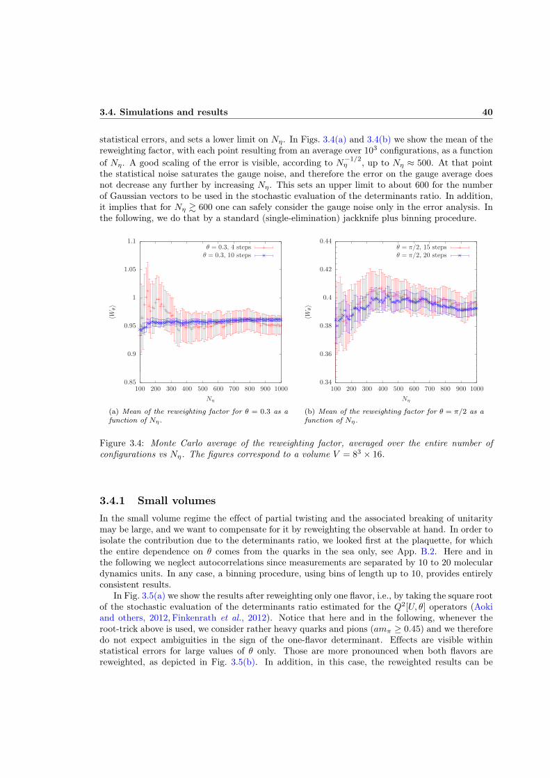
3.4. Simulations and results 40
statistical errors, and sets a lower limit on Nη. In Figs. 3.4(a) and 3.4(b) we show the mean of thereweighting factor, with each point resulting from an average over 103 configurations, as a functionof Nη. A good scaling of the error is visible, according to N−1/2
η , up to Nη ≈ 500. At that pointthe statistical noise saturates the gauge noise, and therefore the error on the gauge average doesnot decrease any further by increasing Nη. This sets an upper limit to about 600 for the numberof Gaussian vectors to be used in the stochastic evaluation of the determinants ratio. In addition,it implies that for Nη & 600 one can safely consider the gauge noise only in the error analysis. Inthe following, we do that by a standard (single-elimination) jackknife plus binning procedure.
θ = 0.3, 10 stepsθ = 0.3, 4 steps
Nη
〈Wθ〉
1000900800700600500400300200100
1.1
1.05
1
0.95
0.9
0.85
(a) Mean of the reweighting factor for θ = 0.3 as afunction of Nη.
θ = π/2, 20 stepsθ = π/2, 15 steps
Nη
〈Wθ〉
1000900800700600500400300200100
0.44
0.42
0.4
0.38
0.36
0.34
(b) Mean of the reweighting factor for θ = π/2 as afunction of Nη.
Figure 3.4: Monte Carlo average of the reweighting factor, averaged over the entire number ofconfigurations vs Nη. The figures correspond to a volume V = 83 × 16.
3.4.1 Small volumesIn the small volume regime the effect of partial twisting and the associated breaking of unitaritymay be large, and we want to compensate for it by reweighting the observable at hand. In order toisolate the contribution due to the determinants ratio, we looked first at the plaquette, for whichthe entire dependence on θ comes from the quarks in the sea only, see App. B.2. Here and inthe following we neglect autocorrelations since measurements are separated by 10 to 20 moleculardynamics units. In any case, a binning procedure, using bins of length up to 10, provides entirelyconsistent results.
In Fig. 3.5(a) we show the results after reweighting only one flavor, i.e., by taking the square rootof the stochastic evaluation of the determinants ratio estimated for the Q2[U, θ] operators (Aokiand others, 2012, Finkenrath et al., 2012). Notice that here and in the following, whenever theroot-trick above is used, we consider rather heavy quarks and pions (amπ ≥ 0.45) and we thereforedo not expect ambiguities in the sign of the one-flavor determinant. Effects are visible withinstatistical errors for large values of θ only. Those are more pronounced when both flavors arereweighted, as depicted in Fig. 3.5(b). In addition, in this case, the reweighted results can be
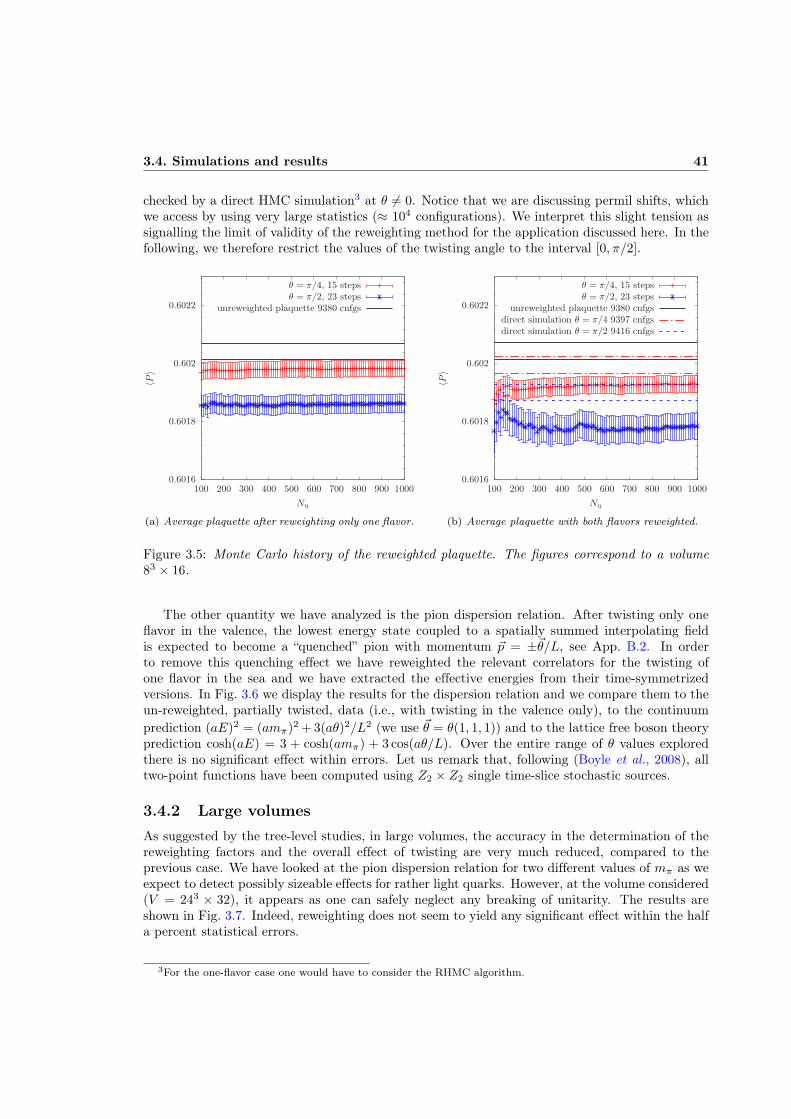
3.4. Simulations and results 41
checked by a direct HMC simulation3 at θ 6= 0. Notice that we are discussing permil shifts, whichwe access by using very large statistics (≈ 104 configurations). We interpret this slight tension assignalling the limit of validity of the reweighting method for the application discussed here. In thefollowing, we therefore restrict the values of the twisting angle to the interval [0, π/2].
unreweighted plaquette 9380 cnfgsθ = π/2, 23 stepsθ = π/4, 15 steps
Nη
〈P〉
1000900800700600500400300200100
0.6022
0.602
0.6018
0.6016
(a) Average plaquette after reweighting only one flavor.
direct simulation θ = π/2 9416 cnfgsdirect simulation θ = π/4 9397 cnfgsunreweighted plaquette 9380 cnfgs
θ = π/2, 23 stepsθ = π/4, 15 steps
Nη
〈P〉
1000900800700600500400300200100
0.6022
0.602
0.6018
0.6016
(b) Average plaquette with both flavors reweighted.
Figure 3.5: Monte Carlo history of the reweighted plaquette. The figures correspond to a volume83 × 16.
The other quantity we have analyzed is the pion dispersion relation. After twisting only oneflavor in the valence, the lowest energy state coupled to a spatially summed interpolating fieldis expected to become a “quenched” pion with momentum ~p = ±~θ/L, see App. B.2. In orderto remove this quenching effect we have reweighted the relevant correlators for the twisting ofone flavor in the sea and we have extracted the effective energies from their time-symmetrizedversions. In Fig. 3.6 we display the results for the dispersion relation and we compare them to theun-reweighted, partially twisted, data (i.e., with twisting in the valence only), to the continuumprediction (aE)2 = (amπ)2 + 3(aθ)2/L2 (we use ~θ = θ(1, 1, 1)) and to the lattice free boson theoryprediction cosh(aE) = 3 + cosh(amπ) + 3 cos(aθ/L). Over the entire range of θ values exploredthere is no significant effect within errors. Let us remark that, following (Boyle et al., 2008), alltwo-point functions have been computed using Z2 × Z2 single time-slice stochastic sources.
3.4.2 Large volumesAs suggested by the tree-level studies, in large volumes, the accuracy in the determination of thereweighting factors and the overall effect of twisting are very much reduced, compared to theprevious case. We have looked at the pion dispersion relation for two different values of mπ as weexpect to detect possibly sizeable effects for rather light quarks. However, at the volume considered(V = 243 × 32), it appears as one can safely neglect any breaking of unitarity. The results areshown in Fig. 3.7. Indeed, reweighting does not seem to yield any significant effect within the halfa percent statistical errors.
3For the one-flavor case one would have to consider the RHMC algorithm.

3.5. Quark mass dependence on the twisting angle 42
lattice free curvecontinuum
reweighted datapartially twisted data
θ/L
aE(θ)
0.20.150.10.050
1.03
1.02
1.01
1
0.99
0.98
0.97
0.96
0.95
Figure 3.6: Pion dispersion relation for V = 83 × 16. Each point is obtained with a different(growing with θ) number of independent steps in the determination of the reweighting factor andNη & 600 in each step.
lattice free curvecontinuum curvereweighted data
partially twisted data
θ/L
aE(θ)
0.060.050.040.030.020.010
0.745
0.74
0.735
0.73
0.725
(a) “Heavy” case of m0 ' −0.65.
lattice free curvecontinuum curvereweighted data
partially twisted data
θ/L
aE(θ)
0.060.050.040.030.020.010
0.465
0.46
0.455
0.45
0.445
0.44
0.435
(b) “Light” case of m0 ' −0.72.
Figure 3.7: Pion dispersion relation for V = 243×32. The reweighting factor at a given θ is obtainedby a telescopic product involving all the previous ones, each one estimated using Nη & 600.
3.5 Quark mass dependence on the twisting angleAs mentioned above, non-periodic boundary conditions (θ 6= 0) for fermionic fields are equivalent tointroducing a constant U(1) interaction, through an external field Bµ(x) = Bµ coupled to periodicfermions. That amounts to replacing the links Uµ with the links Uµ given by
Uµ(x) = eiaBµUµ(x) , (3.5.17)

3.5. Quark mass dependence on the twisting angle 43
where Bµ = θµ/Lµ. In this case the PCAC relation remains unaffected since the new linksUµ(x), being proportional to the identity in flavor, still commute with the Pauli matrices4. Thatimplies that the vector transformations are still exact symmetries at finite lattice spacing withWilson fermions, and that the PCAC relation remains formally the same. Cutoff effects on theother hand depend on the choice of boundary conditions, that has actually been exploited inorder to compute improvement coefficients (see, for example, Refs. (Luscher et al., 1997,Durr andDella Morte, 2004)), within the Symanzik improvement programme for Wilson fermions in QCD.In some instances, even after improvement, the quark mass defined through the PCAC relation inrather small volumes, turned out to have a quite pronounced residual (i.e., O(a2)) dependence onthe boundary conditions (Sommer et al., 2004). That is expected to be even larger here, with un-improved Wilson fermions. For completeness, the bare PCAC quark mass mPCAC can be definedthrough the spatially integrated axial Ward identity as:
mPCAC =∂0〈A0(x0)O(0)〉2〈P (x0)O(0)〉 , (3.5.18)
with Aµ the axial current, P the pseudoscalar density (both spatially summed over the xth0 time-
slice) and O an interpolating field, which in our case will be simply given by the pseudoscalardensity localized at the origin.
Intermezzo: PCAC with TBCs In the PCAC relation we want the variation of the Wilsonterm to vanish in the naïve continuum limit, a → 0 (see Sect. 1.6.2). Now we have anotherdimension [1] field to take into account with respect to case with no constant U(1) interaction.This means that we can write additional operators that mix with O5. In particular we find,following App. A.3 in the case of degenerate flavors,
O5 = Z5
[O5 +
2m
aP f +
ZA − 1
a∂µA
fµ + 2
(Bµ)2P f + Bµ∂
−µ P
f
], (3.5.19)
where f is a flavor index. By substituting back the above expression in Eq. 1.6.52 we obtain
∂−µ 〈Afµ(x)O(y)〉 = 2(m0 −m− aBµBµ
)〈P f (x)O(y)〉 − aBµ∂−µ 〈P f (x)O(y)〉+ 〈χfA(x)O(y)〉.
(3.5.20)
One of the two extra term, compared to Eq. 1.6.54, is vanishing when we consider the integratedWTI. In particular by projecting to zero momentum we find that the following integral is vanishing(B0 = 0)
aBj
∫d3x ∂−j 〈P f (x)O(y)〉 = 0, (3.5.21)
because we have chosen PBCs for our fields.In this case mAWI in Eq. 1.6.55 is given by
mAWI = m0 −m− aB2
j = m0 − f(g0, am0, a2B2
j )/a, (3.5.22)
hence the zero quark mass is attained when the bare mass is equal to the critical value
mc = f(g0, amc, a2B2
j )/a , (3.5.23)
4We are working with two degenerate massive flavors, i.e. the isosymmetric limit.

3.5. Quark mass dependence on the twisting angle 44
which is a function of g0 and B2j = θ2
j/L2 bare parameters. We should note that the function f
depends on quadratically on Bj due to Lorentz invariance.
For the present discussion, it is useful to introduce θv as the spatially isotropic twisting angleused for all fermions in the valence and θs as the corresponding one for all fermions in the sea. Weproduced small volume configurations for different values of θs and on those we measured quarkand pion masses while changing θv. That can actually be used to get an idea of what the effect ofreweighting should be, and we will see that the observations above are confirmed. In particular,at fixed θv, results depend at most at the percent level only on θs.
In Fig. 3.8 we show the pion effective masses computed on about 4000 independent configura-tions generated for lattices of size 83 × 32 at β = 2.2 and m0 = −0.72. All the results in the leftpanel refer to unitary points, i.e. θs = θv. Naively one would expect the results to lie on top of eachother as they all correspond to zero-momentum pions at the same bare parameters. We ascribe thedifference to the dependence of the critical bare mass mc on both θs and θv, as explained above.Since mc is obtained from the PCAC operator identity the dependence on the twisting angles isa boundary, therefore finite volume, cutoff effect. This explains why the continuum dispersionrelation is rather poorly reproduced in small volumes and for large values of the twisting angle, asshown in Fig. 3.6. Upon twisting, not only the pions get boosted, but also at least one of the quarkmasses decreases, such that the two effects partly compensate. In the right panel of Fig. 3.8 thefinal estimates of the masses are shown as a function of θ = θv. The square points are the unitaryones, corresponding to the plateaux in the left panel, whereas the triangle ones are obtained byusing configurations produced at θs = 0 on which two-point functions are computed for differentvalues of θv = θ. It is clear that by reweighting the sea twisting angle to the valence one at mosta percent effect could have been produced here in the case θs = 0, θv = π/2.
θ = π/2θ = π/4
θ = 0
m = −0.72
t
am
eff
π(t)
16151413121110987
0.9
0.85
0.8
0.75
0.7
0.65
0.6
0.55
0.5
partially twisted datagenerated data
m = −0.72
θ
am
π
π/23π/8π/4π/80
0.9
0.85
0.8
0.75
0.7
0.65
0.6
0.55
0.5
Figure 3.8: Pion effective masses for θs = θv = θ on a 83 × 32 lattice at β = 2.2, m0 = −0.72 (leftpanel) and comparison of the corresponding plateau masses (red) with the result from θs = 0 as afunction of θ = θv (right panel).
The bare PCAC quark mass, in the un-improved theory, can be related to the bare parameter

3.6. Conclusions 45
m0 asmPCAC(β, θ) = Z(β, θ) (m0 −mc(β, θ)) , (3.5.24)
where Z is a normalization factor and mc is the value of the bare mass parameter defining themassless limit. As a consequence of the breaking of chiral symmetry with Wilson fermions mc isdifferent from zero, as opposite to the case of Ginsparg-Wilson or staggered fermions, where at leastsome axial transformations are preserved and that is enough to rule out an additive renormalizationof the bare mass. We are here restricting the attention to the case θs = θv = θ and we are workingat fixed β. By looking at mPCAC as a function of m0, for m0 slightly larger than mc, one obtains afamily of linear curves parameterized by θ. The slope of the curves is given by Z, while the valueof m0 where the curves intercept the horizontal axis corresponds to mc. That is exactly whatis shown in Fig. 3.9 for m0 = −0.72, −0.735 and −0.75 (with β fixed to 2.2 and V = 83 × 32).Whereas the dependence of Z on θ is not significant, mc, as anticipated, changes substantially withthe twisting angle. At θ = π/2 and for m0 = −0.75 the PCAC mass is roughly one half of the valueat θ = 0. We find that corresponding ratio for pion masses is within 1.5 and 1.7, which, given thesmall volumes we have considered, is quite consistent with the scaling in a chirally broken theory.
θ = π/2θ = π/4θ = 0
m0
mPCAC
−0.72−0.73−0.74−0.75−0.76−0.77
0.07
0.06
0.05
0.04
0.03
0.02
0.01
0
−0.01
−0.02
Figure 3.9: mPCAC as a function of m0 computed for m0 = −0.72, −0.735 and −0.75 at β = 2.2and V = 83 × 16. The curves correspond to three different values of θ = θv = θs.
Finally, let us remark that similar shifts in the quark mass have been discussed for the case ofconstant external magnetic fields (Brandt et al., 2016). We emphasize that here we are showingthat such effects are present also in the case of vanishing magnetic field and constant (vector)potential.
3.6 ConclusionsWe explored in detail an application of reweighting techniques to the case of modifications in thespatial periodicity of fermions. We have thoroughly studied the approach at tree-level and we have

3.6. Conclusions 46
provided constraints for the convergence of the stochastic estimates of all the Gaussian momentsof the reweighting factors. We have also established the large volume scaling of the average andthe variance at tree-level.
At the numerical level, we have performed a complete and detailed study of purely gluonic aswell as fermionic quantities in both large and small volumes. We considered the plaquette andthe pion dispersion relation, the latter in the two regimes. In both cases we found the effectsof reweighting to be at the sub-percent level for values of θ up to π/2. In our implementation,for the large volumes considered, we found that the reweighting method, with Nη ≈ 600 is afactor 4-5 cheaper compared to generating new configurations for different values of the twistingangle, assuming that about 20 molecular dynamics units are needed to decorrelate subsequentconfigurations. We performed this comparison in units of matrix-vector multiplications.
Perhaps the most important observation, which, as far as we know, has so far not been inves-tigated in a dedicated way in the literature, is on the dependence of the critical mass for Wilsonfermions on the periodicity phases in the boundary conditions. Although a cutoff effect, it could berather large in a theory with O(a) discretization effects. Since the result is that the hadron masses,and not only their momentum, change as θ changes, the corresponding dispersion relations maylook very different at finite and coarse lattice spacings compared to the continuum predictions.

Chapter 4
Optimization of HMC performance
Gauge theories formulated on Euclidean lattices can be treated as statistical system and areamenable to numerical simulations. When matter fields (scalars or fermions) are dynamicallypresent, the gauge-field configurations are typically generated using Molecular Dynamics (MD) al-gorithms, which come with different variantions of the Hybrid Monte Carlo (HMC) (Duane et al.,1987). Such algorithms depend on a large number of parameters, whose optimal choices dependon the model and the regime (e.g. concerning masses and volumes) considered. The generation ofconfigurations in large volumes at light quark masses is still very demanding. For larger volumesthe simulations become obviously more expensive. For lighter quarks the condition number ofthe Dirac operator increases, hence the number of iterations needed by the solver (to invert theoperator) increases.
The case of QCD has been extensively studied because of its obvious phenomenological rele-vance. Roughly speaking HMC algorithms can be classified according to the factorization of thequark determinant adopted (tipically either mass-preconditioning (Hasenbusch, 2001), or even/oddpreconditioning (DeGrand and Rossi, 1990), or domain-decomposition (Luscher, 2005), or rationalfactorization (Clark and Kennedy, 2007)) and the symplectic integrator(s) used, the simplest beingthe leapfrog integrator, and the most popular being the second order minimum norm integratoror Omelyan integrator (Omelyan et al., 2003,Takaishi and de Forcrand, 2006). The factorizationof the determinant translates into a splitting of fermionic forces in the Molecular Dynamics, anddepending on the hierarchy of such forces various nested integrators can be used, where each forceis integrated along a trajectory with a different time-step (Sexton and Weingarten, 1992,Urbach etal., 2006). No complete studies are present for Beyond Standard Model (BSM) strongly interactingmodels, where the hierarchy of the forces can be completely different from the QCD case.
In dynamical simulations the Molecular Dynamics step is the most time consuming part, henceit is of paramount importance to speed it up as much as possible. For symplectic integrators ashadow Hamiltonian exists, that is conserved, and can be used to optimize the parameters of asimulation. In Ref. (Kennedy and Clark, 2007) the shadow Hamiltonian was introduced to makesimulations with dynamical fermions cheaper by means of symplectic integrators that conservein a better way the energy without decreasing the integration step-size too much. The idea inthe present work is to minimize the fluctuations of the Hamiltonian deviations from the shadowHamiltonian along the trajectory. The strategy we will follow is general and it is also suitable forBSM models.In the following we restrict the attention to the case of one particular integrator, Omelyan (withα = 1/6), because it is a rather common choice, requires less computations and existing data (aslong as the norm of the forces have been stored) can be readily used for the tuning. We employ
47

4.1. Symplectic integrators: a toy model 48
a three-time scale integrator with mass-preconditioning and we show that once the forces andtheir variances are measured, assuming they only depend on the mass-preconditioning parameterµ (and bare mass parameter m0 − mc), we are able to find the optimal integrator parameters.Thanks to choice of α = 1/6 in the integrator, the implementation of the Poisson brackets isnot needed since their rôle is played by the forces. It should be noted that the tuning of theintegrator parameters also depends on the choice of the inverter, the precision of the force andthe Hamiltonian measurement. The strategy we present is applicable also for a different set ofthe aforementioned choices. Our minimization method gives predictions accurate at the 10% level,which we consider quite satisfactory. For completeness we consider an SU(2) gauge group with adoublet of un-improved Wilson fermions in the fundamental representation and Wilson plaquettegauge action, further details on the simulations set-up can be found in App. C.4.
The chapter is organized as follow; in Section 1 we review symplectic integrators and theexistence of a shadow Hamiltonian associated to them for the case of position and momentumvariables in R2. In Section 2 we give our set-up for the integrator, preconditioning and multi-scaleintegration and we show the explicit form of the shadow Hamiltonian and how it depends on theforces. In Section 3 we test the goodness of our measurement of Poisson brackets and we showthat the shadow Hamiltonian is indeed conserved along the trajectory. In Section 4 we relate theacceptance rate in simulations to the variance of the shadow Hamiltonian and ultimately to theforce variances; the cost of a simulation is also defined. There we also present the functional formof the fits employed in µ (and the bare mass m0). Section 5 contains the comparison of the costof actual simulation with the one found through our minimization method. Section 6 contains ourconclusions. The work presented in this chapter is presented in (Bussone et al., 2016a).
4.1 Symplectic integrators: a toy modelTo each symplectic integrator corresponds a constant of motion related to the original Hamiltonianof the system we want to simulate. The constant of motion is referred to as shadow Hamiltonian.See Ref. (Yoshida, 1992) for a review. Let us examine the case of the 1D harmonic oscillator. TheHamiltonian of such a system is
H =p2
2+q2
2, (4.1.1)
and the exact solution is given by the following map(p′
q′
)=
(cos τ − sin τsin τ cos τ
)(p(0)q(0)
), (4.1.2)
where (q(0), p(0)) is the initial condition and (q′, p′) is the τ -time evolved point in the phase space(q, p). Without loss of generality let us assume τ > 1.
EulerThe easiest way to solve the differential equation numerically is to employ the Euler method. Inthat case the map is given by
(p′
q′
)=
(1 −ττ 1
)(p(0)q(0)
). (4.1.3)
The map is not symplectic and the time evolved Hamiltonian is found to be
H(τ) = H(0) +τ2
2
[p2(τ) + q2(τ)
]6= H(0). (4.1.4)
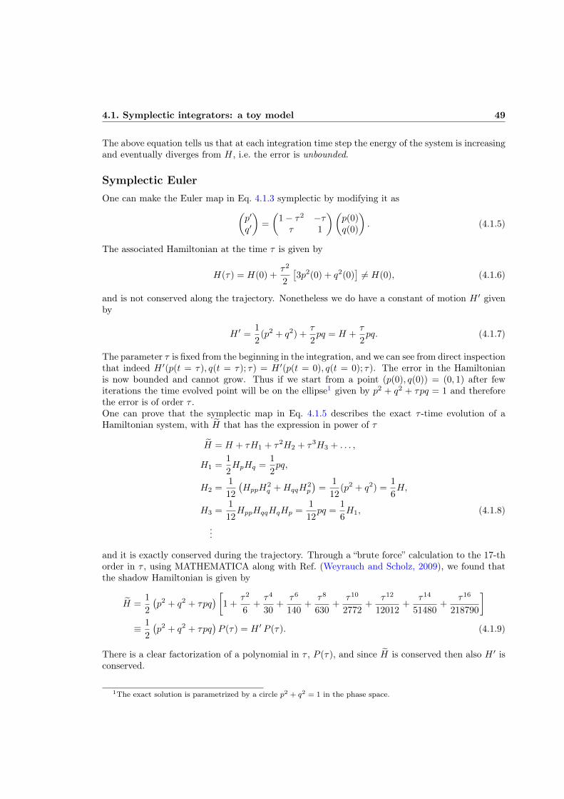
4.1. Symplectic integrators: a toy model 49
The above equation tells us that at each integration time step the energy of the system is increasingand eventually diverges from H, i.e. the error is unbounded.
Symplectic EulerOne can make the Euler map in Eq. 4.1.3 symplectic by modifying it as
(p′
q′
)=
(1− τ2 −ττ 1
)(p(0)q(0)
). (4.1.5)
The associated Hamiltonian at the time τ is given by
H(τ) = H(0) +τ2
2
[3p2(0) + q2(0)
]6= H(0), (4.1.6)
and is not conserved along the trajectory. Nonetheless we do have a constant of motion H ′ givenby
H ′ =1
2(p2 + q2) +
τ
2pq = H +
τ
2pq. (4.1.7)
The parameter τ is fixed from the beginning in the integration, and we can see from direct inspectionthat indeed H ′(p(t = τ), q(t = τ); τ) = H ′(p(t = 0), q(t = 0); τ). The error in the Hamiltonianis now bounded and cannot grow. Thus if we start from a point (p(0), q(0)) = (0, 1) after fewiterations the time evolved point will be on the ellipse1 given by p2 + q2 + τpq = 1 and thereforethe error is of order τ .One can prove that the symplectic map in Eq. 4.1.5 describes the exact τ -time evolution of aHamiltonian system, with H that has the expression in power of τ
H = H + τH1 + τ2H2 + τ3H3 + . . . ,
H1 =1
2HpHq =
1
2pq,
H2 =1
12
(HppH
2q +HqqH
2p
)=
1
12(p2 + q2) =
1
6H,
H3 =1
12HppHqqHqHp =
1
12pq =
1
6H1, (4.1.8)
...
and it is exactly conserved during the trajectory. Through a “brute force” calculation to the 17-thorder in τ , using MATHEMATICA along with Ref. (Weyrauch and Scholz, 2009), we found thatthe shadow Hamiltonian is given by
H =1
2
(p2 + q2 + τpq
) [1 +
τ2
6+τ4
30+
τ6
140+
τ8
630+
τ10
2772+
τ12
12012+
τ14
51480+
τ16
218790
]
≡ 1
2
(p2 + q2 + τpq
)P (τ) = H ′ P (τ). (4.1.9)
There is a clear factorization of a polynomial in τ , P (τ), and since H is conserved then also H ′ isconserved.
1The exact solution is parametrized by a circle p2 + q2 = 1 in the phase space.

4.1. Symplectic integrators: a toy model 50
4.1.1 Shadow hamiltonianThe Hamilton equations in compact form are given by
dzdt
= z,H(z) ≡ DHz. (4.1.10)
where we introduced z ∈ R2n = (p, q), and the Poisson brackets are given by
?,H =∂?
∂q
∂H
∂p− ∂?
∂p
∂H
∂q. (4.1.11)
The formal solution of the differential equation takes the form z(τ) = eτDHz(0). By choosing aseparable Hamiltonian, H(q, p) = T (p)+V (q), we have the operator identification DH = DT +DV
and the solution can be formally written through the evolution operator as follows
z(τ) = eτ(DT+DV )z(0). (4.1.12)
More explicitly
momenta evolution eτDV : f(z(0)) = f(p, q)→ f(z(τ)) = f(p− τVq, q),positions evolution eτDT : f(z(0)) = f(p, q)→ f(z(τ)) = f(p, q + τTp), (4.1.13)
where f is an arbitrary function of z.Let us specialize to the Omelyan integrator (Omelyan et al., 2003). The evolution operator in thiscase is
exp[ατDV ] exp[τ
2DT
]exp [τ(1− 2α)DV ] exp
[τ2DT
]exp[ατDV ], (4.1.14)
with α free parameter. By using the Baker-Campbell-Haussdorff (BCH) formula we obtain thatthe shadow Hamiltonian H is related to the one we want to simulate, H, as follows
H = H + τ2
6α2 − 6α+ 1
12DV [DV (T )] +
1− 6α
24DT [DV (T )]
+ O(τ4). (4.1.15)
By putting α = 1/6 the second term in curly brackets vanishes. The remainder is proportional toDV [DV (T )]. In the case of V = V (q) and T = p2/2 this operator is related to the force,
DV (T ) = T, V =VpTq − VqTp = −pVq,
DV [DV (T )] = −pVq, V = V, pVq = Vq(pVq)p −Vp(pVq)q = Vq(Vq +pVqp ) = V 2
q ≡ F 2.
(4.1.16)
The shadow Hamiltonian in the case of Omelyan integrator with α = 1/6 is given by
H = H +(τF )2
72+ O(τ4). (4.1.17)
Time reversible integratorsLet us assume we have a time reversible integrator given by
E(τ) = exp (τA) exp (τB) , (4.1.18)
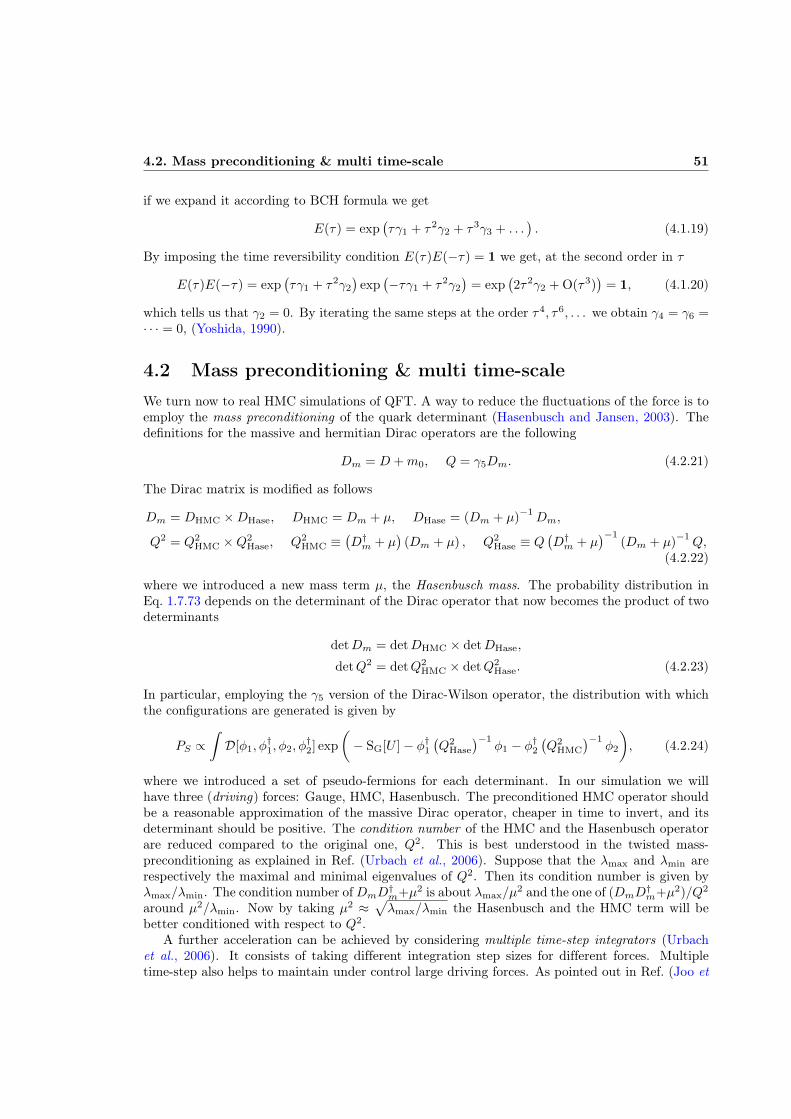
4.2. Mass preconditioning & multi time-scale 51
if we expand it according to BCH formula we get
E(τ) = exp(τγ1 + τ2γ2 + τ3γ3 + . . .
). (4.1.19)
By imposing the time reversibility condition E(τ)E(−τ) = 1 we get, at the second order in τ
E(τ)E(−τ) = exp(τγ1 + τ2γ2
)exp
(−τγ1 + τ2γ2
)= exp
(2τ2γ2 + O(τ3)
)= 1, (4.1.20)
which tells us that γ2 = 0. By iterating the same steps at the order τ4, τ6, . . . we obtain γ4 = γ6 =· · · = 0, (Yoshida, 1990).
4.2 Mass preconditioning & multi time-scaleWe turn now to real HMC simulations of QFT. A way to reduce the fluctuations of the force is toemploy the mass preconditioning of the quark determinant (Hasenbusch and Jansen, 2003). Thedefinitions for the massive and hermitian Dirac operators are the following
Dm = D +m0, Q = γ5Dm. (4.2.21)
The Dirac matrix is modified as follows
Dm = DHMC ×DHase, DHMC = Dm + µ, DHase = (Dm + µ)−1Dm,
Q2 = Q2HMC ×Q2
Hase, Q2HMC ≡
(D†m + µ
)(Dm + µ) , Q2
Hase ≡ Q(D†m + µ
)−1(Dm + µ)
−1Q,
(4.2.22)
where we introduced a new mass term µ, the Hasenbusch mass. The probability distribution inEq. 1.7.73 depends on the determinant of the Dirac operator that now becomes the product of twodeterminants
detDm = detDHMC × detDHase,
detQ2 = detQ2HMC × detQ2
Hase. (4.2.23)
In particular, employing the γ5 version of the Dirac-Wilson operator, the distribution with whichthe configurations are generated is given by
PS ∝∫D[φ1, φ
†1, φ2, φ
†2] exp
(− SG[U ]− φ†1
(Q2
Hase
)−1φ1 − φ†2
(Q2
HMC
)−1φ2
), (4.2.24)
where we introduced a set of pseudo-fermions for each determinant. In our simulation we willhave three (driving) forces: Gauge, HMC, Hasenbusch. The preconditioned HMC operator shouldbe a reasonable approximation of the massive Dirac operator, cheaper in time to invert, and itsdeterminant should be positive. The condition number of the HMC and the Hasenbusch operatorare reduced compared to the original one, Q2. This is best understood in the twisted mass-preconditioning as explained in Ref. (Urbach et al., 2006). Suppose that the λmax and λmin arerespectively the maximal and minimal eigenvalues of Q2. Then its condition number is given byλmax/λmin. The condition number ofDmD
†m+µ2 is about λmax/µ
2 and the one of (DmD†m+µ2)/Q2
around µ2/λmin. Now by taking µ2 ≈√λmax/λmin the Hasenbusch and the HMC term will be
better conditioned with respect to Q2.A further acceleration can be achieved by considering multiple time-step integrators (Urbach
et al., 2006). It consists of taking different integration step sizes for different forces. Multipletime-step also helps to maintain under control large driving forces. As pointed out in Ref. (Joo et

4.3. Benchmarks in small volumes 52
al., 2000) large driving forces lead to instabilities in HMC simulations. To avoid them the timestep must be small if the driving force are large. Multiple time-step integrators are a valuable toolif the forces differ by orders of magnitude in absolute value.We employ a three time-scale integrator and assume that in the outermost level there is theevolution for S1 with time step δτ = τ/n, in the middle the integrator for S2 with m steps and theinnermost is for S3 with k steps.
The shadow Hamiltonian associated to the Omelyan integrator with three time-scales and masspreconditioning is a quite lengthy expression (see App. C.3) but once we set the parameter α = 1/6it is given by
H = H +δτ2
72
[[S1, [S1, T ]] +
1
4m2[S2, [S2, T ]] +
1
16m2k2[S3, [S3, T ]]
]+ O(δτ4). (4.2.25)
We use the conventions adopted in (Kennedy et al., 2013,Kennedy and Clark, 2007) and the aboveformula becomes
H = H +δτ2
72
[ei (S1) ei (S1) +
ei (S2) ei (S2)
4m2+
ei (S3) ei (S3)
16m2k2
]+ O(δτ4), (4.2.26)
where ei is the SU(Nc) derivative and i a collective index for space-time, direction and number ofgenerators. ei(S)ei(S) gives the force associated to the action S summed over all space-time point,directions, color and eventually spin, as expected, since the Hamiltonian is an extensive quantity.The shadow Hamiltonian reduces to
H = H +δτ2
72
∑
x,µ,a
[TR,1 (F aµ1 (x))
2+ TR,2
(F aµ2 (x))2
4m2+ TR,3
(F aµ3 (x))2
16m2k2
]+ O(δτ4)
≡ H +δτ2
72
(|F1|2 +
|F2|24m2
+|F3|2
16m2k2
)+ O(δτ4) ≡ H + δH + O(δτ4), (4.2.27)
that is a function only of the forces used during the simulations.For the derivation of the various forces see the results in App. C.3. We immediately see that theshadow Hamiltonian is related to the different parts of the force weighted by the correspondingnormalization for the generators TR in the given representation R. Note that the gauge is alwaysin the fundamental TR = Tf = 1/2, while the fermionic parts may be in different representation.Already at this point one can see what drove our assignments for the different levels. We wantto suppress the contribution of the largest force (the gauge one) and hence that will go in theinnermost level, followed by the HMC force and the Hasenbusch one at the outermost level.
In the following we specialize to the case of the Omelyan integrator with α = 1/6. We con-sider an SU(2) gauge group with a doublet of un-improved Wilson fermions in the fundamentalrepresentation and Wilson plaquette gauge action. For completeness the value mc of the baremass parameter yielding massless fermions is estimated to be −0.77(2) at β = 2.2 (Lewis et al.,2012,Hietanen et al., 2014,Arthur et al., 2016).
4.3 Benchmarks in small volumesIn order to test the measurements of the Poisson brackets we check the scaling with δτ of |∆H| ∝δτ2, since the Omelyan integrator is a second order integrator. Furthermore we test the scalingof |∆(δH) + ∆H| ∝ δτ4, indeed, since H is conserved along the trajectory, the following relationholds
∆H = 0 = ∆H + ∆(δH) + O(δτ4) =⇒ ∆H = −∆(δH) + O(δτ4). (4.3.28)

4.3. Benchmarks in small volumes 53
The difference at the end of the trajectory is given by
∆(δH) =δτ2
72
(|F1,f |2 − |F1,i|2 +
|F2,f |2 − |F2,i|24m2
+|F3,f |2 − |F3,i|2
16m2k2
), (4.3.29)
where the forces are evaluated at the beginning i and the end f of the trajectory.For the tests we have run one trajectory from a thermalized configuration with the following set-upfor the levels in the integration, τf = 1,
• level 1: Hasenbusch, n = 4, 5, . . . , 20,
• level 2: HMC, m = 10,
• level 3: Gauge, k = 10.
The results in small volumes are shown in Fig. 4.1. In Fig. 4.1(b) we see in the small δτ region theemergence of a contribution of order δτ3. This comes from the ambiguity in the measurement of
δτ4|∆(δH) + ∆H |
δτ2|∆H |
µ = 0.2, Volume 84 HMC steps 10, Gauge steps 10
δτ
10.10.01
10−1
10−2
10−3
10−4
10−5
10−6
(a) Scaling of |∆H| and |∆(δH)+∆H| with δτin V = 84 at fixed inner levels steps m = 10and k = 10.
δτ3δτ4
m = 10, k = 10m = 4, k = 4
Volume 44, µ = 0.05
δτ = 1/n
|∆(δH)−∆H|
0.10.01
1.0e-02
1.0e-03
1.0e-04
1.0e-05
1.0e-06
1.0e-07
(b) Scaling of |∆(δH) + ∆H| with δτ in V = 44 for twodifferent choices of the inner level steps.
Figure 4.1: Scaling behavior with δτ = 1/n for ∆H and ∆(δH) in small volumes. ∆(δH) is builtfrom the knowledge of the forces at the beginning and the end of the trajectory. Lines are shown toguide the eye.
F2, that is the time in which we measure it in the sub-level steps. In other words different forcesare measured at different times. In formulae we can write
|F2|2 = |Fm→∞2 |2 + O(δτ
m
), (4.3.30)
where δτ/m gives a correction to δH of order 1/m3. This term induces a contribution of orderδτ3 in |∆(δH) + ∆H| that can be suppressed by choosing a large number of steps m. The same
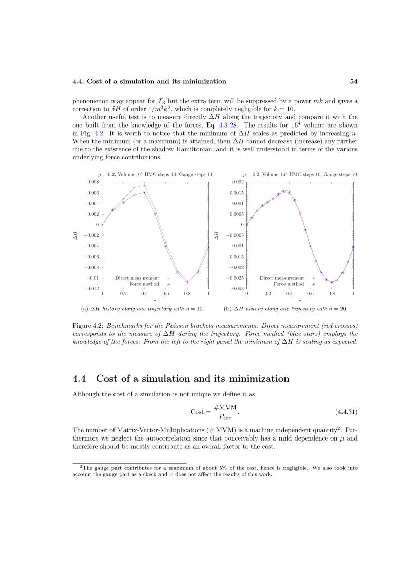
4.4. Cost of a simulation and its minimization 54
phenomenon may appear for F3 but the extra term will be suppressed by a power mk and gives acorrection to δH of order 1/m3k3, which is completely negligible for k = 10.
Another useful test is to measure directly ∆H along the trajectory and compare it with theone built from the knowledge of the forces, Eq. 4.3.28. The results for 164 volume are shownin Fig. 4.2. It is worth to notice that the minimum of ∆H scales as predicted by increasing n.When the minimum (or a maximum) is attained, then ∆H cannot decrease (increase) any furtherdue to the existence of the shadow Hamiltonian, and it is well understood in terms of the variousunderlying force contributions.
Force methodDirect measurement
µ = 0.2, Volume 164 HMC steps 10, Gauge steps 10
τ
∆H
10.80.60.40.20
0.008
0.006
0.004
0.002
0
−0.002
−0.004
−0.006
−0.008
−0.01
−0.012
(a) ∆H history along one trajectory with n = 10.
Force methodDirect measurement
µ = 0.2, Volume 164 HMC steps 10, Gauge steps 10
τ
∆H
10.80.60.40.20
0.002
0.0015
0.001
0.0005
0
−0.0005
−0.001
−0.0015
−0.002
−0.0025
−0.003
(b) ∆H history along one trajectory with n = 20.
Figure 4.2: Benchmarks for the Poisson brackets measurements. Direct measurement (red crosses)corresponds to the measure of ∆H during the trajectory. Force method (blue stars) employs theknowledge of the forces. From the left to the right panel the minimum of ∆H is scaling as expected.
4.4 Cost of a simulation and its minimizationAlthough the cost of a simulation is not unique we define it as
Cost =#MVM
Pacc. (4.4.31)
The number of Matrix-Vector-Multiplications (# MVM) is a machine independent quantity2. Fur-thermore we neglect the autocorrelation since that conceivably has a mild dependence on µ andtherefore should be mostly contribute as an overall factor to the cost.
2The gauge part contributes for a maximum of about 5% of the cost, hence is negligible. We also took intoaccount the gauge part as a check and it does not affect the results of this work.

4.4. Cost of a simulation and its minimization 55
4.4.1 Acceptance & Matrix-Vector-MultiplicationWe link the acceptance Pacc to ∆H through the Creutz formula, see App. C.1,
Pacc(∆H) = erfc(√
Var(∆H)/8), (4.4.32)
and the connection between the variances of ∆H and δH is given by (Clark et al., 2008,Clark etal., 2011)
Var(∆H) ' 2Var(δH). (4.4.33)
In the following our goal is to optimize the choice of parameters µ, n,m, k, (for different baremasses m0), while keeping the choice of the integrator, the solver and the number of Hasenbuschsplittings fixed. We can also fix the bare masses, but a stabilization in terms of χ-square of thefits is seen once we fit also in m0. But we should mention that it is not strictly necessary.Let us illustrate how to get to the above relation Eq. 4.4.33. We trade ∆H for ∆(δH) throughEq. 4.3.28. By using Eq. 4.3.29 we can compute the variance (and neglecting all the covariances),
Var [∆(δH)] ≡ δτ4
(72)2
[Var
(|F1,f |2
)+ Var
(|F1,i|2
)+
Var(|F2,f |2
)+ Var
(|F2,i|2
)
(4m2)2
+Var
(|F3,f |2
)+ Var
(|F3,i|2
)
(16m2k2)2
]. (4.4.34)
Under the further assumption that the final and initial forces are extracted from the same distri-bution, exp(−H)(Clark et al., 2010), and they are independent for long enough trajectories, weobtain
Var [∆(δH)] ' 2 δτ4
(72)2
[Var
(|F1|2
)+
Var(|F2|2
)
(4m2)2+
Var(|F3|2
)
(16m2k2)2
]= 2Var(δH). (4.4.35)
We have tested Eq. 4.4.33 by calculating in two different ways the acceptance. We refer to theacceptance calculated with the formula in Eq. 4.4.35 (Var(δH)) as “Force method 1”, while “Forcemethod 2” is used for the acceptance calculated with Eq. 4.4.34 (Var [∆(δH)]). “Force method 1”is the one going to be used in the rest of the work. There the acceptance rate is calculated fromthe variance of δH. For each trajectory we calulate the average of δH over each of the uppermostlevel step. The result is then used to build the variance over the trajectories, where the averageforces over the sub-levels are used. In “Force method 2” the acceptance is calculated from thevariance of ∆(δH). To do that we calculate the difference of δH at the beginning and the end ofeach trajectory and we extract the variance over the trajectories. In Fig. 4.3 we compare the twomethods described above to extract the acceptance of a simulation in a small V = 44 volume. Thesimulations are carried out starting from a thermalized configuration and running 103 trajectories.There the two methods are compared with the direct measurement and the acceptance built directlyfrom ∆H. Both methods seem to reasonably reproduce the data.
The total average number of MVM is given in terms of the averages at each level by
#MVM = (2n+ 1)#MVM1(µ) + 2n(2m+ 1)#MVM2(µ). (4.4.36)
The analysis is done with standard statistical error propagation since each simulation, fordifferent choices of n,m, k, µ and m0, is independent.
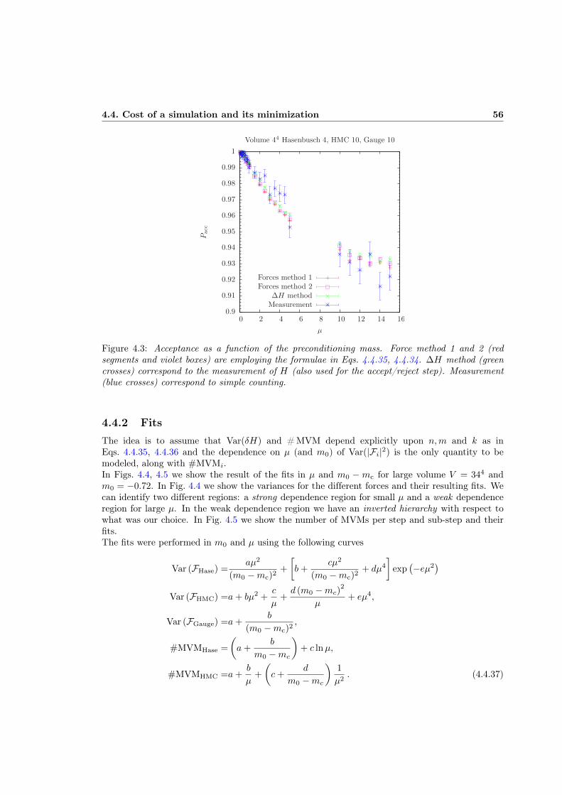
4.4. Cost of a simulation and its minimization 56
Measurement∆H method
Forces method 2Forces method 1
Volume 44 Hasenbusch 4, HMC 10, Gauge 10
µ
Pacc
1614121086420
1
0.99
0.98
0.97
0.96
0.95
0.94
0.93
0.92
0.91
0.9
Figure 4.3: Acceptance as a function of the preconditioning mass. Force method 1 and 2 (redsegments and violet boxes) are employing the formulae in Eqs. 4.4.35, 4.4.34. ∆H method (greencrosses) correspond to the measurement of H (also used for the accept/reject step). Measurement(blue crosses) correspond to simple counting.
4.4.2 FitsThe idea is to assume that Var(δH) and #MVM depend explicitly upon n,m and k as inEqs. 4.4.35, 4.4.36 and the dependence on µ (and m0) of Var(|Fi|2) is the only quantity to bemodeled, along with #MVMi.In Figs. 4.4, 4.5 we show the result of the fits in µ and m0 −mc for large volume V = 344 andm0 = −0.72. In Fig. 4.4 we show the variances for the different forces and their resulting fits. Wecan identify two different regions: a strong dependence region for small µ and a weak dependenceregion for large µ. In the weak dependence region we have an inverted hierarchy with respect towhat was our choice. In Fig. 4.5 we show the number of MVMs per step and sub-step and theirfits.The fits were performed in m0 and µ using the following curves
Var (FHase) =aµ2
(m0 −mc)2+
[b+
cµ2
(m0 −mc)2+ dµ4
]exp
(−eµ2
)
Var (FHMC) =a+ bµ2 +c
µ+d (m0 −mc)
2
µ+ eµ4,
Var (FGauge) =a+b
(m0 −mc)2,
#MVMHase =
(a+
b
m0 −mc
)+ c lnµ,
#MVMHMC =a+b
µ+
(c+
d
m0 −mc
)1
µ2. (4.4.37)
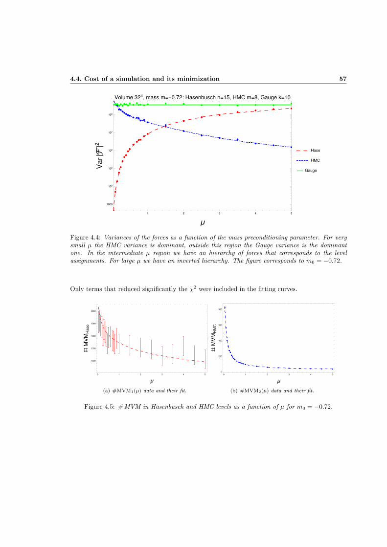
4.4. Cost of a simulation and its minimization 57
1 2 3 4 5
1000
104
105
106
107
108
μ
Var|ℱ
|2Volume 324, mass m=-0.72: Hasenbusch n=15, HMC m=8, Gauge k=10
Hase
HMC
Gauge
Figure 4.4: Variances of the forces as a function of the mass preconditioning parameter. For verysmall µ the HMC variance is dominant, outside this region the Gauge variance is the dominantone. In the intermediate µ region we have an hierarchy of forces that corresponds to the levelassignments. For large µ we have an inverted hierarchy. The figure corresponds to m0 = −0.72.
Only terms that reduced significantly the χ2 were included in the fitting curves.
0 1 2 3 4 5
1600
1700
1800
1900
2000
μ
#M
VM
Hase
(a) #MVM1(µ) data and their fit.
0 1 2 3 4 5
0
200
400
600
800
μ
#M
VM
HM
C
(b) #MVM2(µ) data and their fit.
Figure 4.5: #MVM in Hasenbusch and HMC levels as a function of µ for m0 = −0.72.

4.5. Comparison with simulations 58
4.4.3 Cost functionWe can now build the cost as a function of n,m, k, µ and m0. For simplicity we fix k = 10, and inorder to find the minimum in the other parameters we require3 Pacc & 70%. The minimization iscarried out at fixed bare mass, in the following we specialize to m0 = −0.72 since the results forother bare masses are qualitatively the same. With this set-up we found the minimum, Costmin,to be at (n,m, µ) ≈ (5, 3, 0.3). In Fig. 4.6 we show the cost, normalized to the minimum, andthe acceptance in the plane (µ, n) and (µ,m). In Fig. 4.6(a) we fix m = 3 and it can be seenthat the minimum is close to the boundary Pacc ∼ 70%. By taking the cost of a simulation tobe 1 < Cost/Costmin < 1.25 the window in parameter space is quite broad 0.2 . µ . 0.7 and3 . n . 8. Same conclusions can be drawn for the Fig. 4.6(b).
0.1
0.2
0.3
0.4
0.5
0.6
0.7
0.8
0.9
0.2 0.4 0.6 0.8 1.0
2
4
6
8
10
12
14
μ
1/δτ
Volume 324: HMC m=3, Gauge k=10, Cost, Pacc
1.00
1.25
1.50
1.75
2.00
2.25
2.50
2.75
3.00
(a) Cost/Costmin with m = 3 as function of µ and n.
0.10.1
0.2
0.3
0.4
0.5
0.6
0.7
0.8
0.9
0.2 0.4 0.6 0.8 1.0
2
4
6
8
10
12
14
μ
m
Volume 324: Hasenbusch n=5, Gauge k=10, Cost, Pacc
1.25
1.50
1.75
2.00
2.25
2.50
2.75
3.00
(b) Cost/Costmin with n = 5 as function of µ and n.
Figure 4.6: Ratio Cost/Costmin around the minimum (n,m, µ) ' (5, 3, 0.3) is displayed as curvelevel. Acceptance rate lines are drawn. Bare mass m0 = −0.72.
4.5 Comparison with simulationsWe have run simulations around the minima found with the above methodology for each bare massm0, Tab. 4.1. The results for the cost from simulations and predictions are shown in Fig. 4.7 forthe different m0−mc. Each prediction point represents the minimum cost with different bare massm0, mass-preconditioning µ, number of steps in the uppermost level n and middle level m (k isfixed to 10). The result in Fig. 4.7 represent the central result of this work. It tests the validity ofthe assumptions made so far and it nicely predicts the value of the cost within factors 3 to 4.
3This requirement is needed for the Creutz formula to hold true.

4.6. Conclusions 59
m0 µ n m Ncnf
-0.72 0.29 5 3 463-0.735 0.22 5 3 403-0.75 0.18 5 4 167
Table 4.1: Parameters corresponding to the minimum cost of simulations and number of configu-rations produced.
0.02 0.03 0.04 0.05 0.06
40 000
60 000
80 000
100 000
120 000
140 000
m0-mc
Min
imu
mC
ost
Predictions
Simulations
Figure 4.7: Cost at the minimum, comparison with simulation. Each point correspond to a differentset of parameters µ, n,m. In black comparison with direct simulations is made.
4.6 ConclusionsWe presented a strategy to optimize the parameters of the Omelyan integrator with α = 1/6,Hasenbusch mass preconditioning and three time-scales. We have studied the scaling behavior of∆H in δτ and the goodness of the Poisson brackets measurements through the driving forces in aHMC simulation. We have also generalized the shadow hamiltonian in the presence of multiple-timescales splitting.
We have shown that once the variances of the forces are measured, at fixed bare mass, as afunction of the mass-preconditioning parameter the optimal set-up for the integrator can be found.Our method relies on the existence of a shadow Hamiltonian.We found that the minimum of the cost is quite broad as a function of the mass-preconditioningmass and the number of steps in a level. Nonetheless we are able to give reliable estimates ofthe cost in agreement with actual simulations. An important observation is that we do not needto modify extensively preexisting codes, since practically all of them have to measure the forcesduring a trajectory.
The schematic recipe followed by this work is the following:

4.6. Conclusions 60
• Start with a reasonable choice for the simulation of (n,m, k) at fixed m0.
• Measure the forces in each level, which we already computed for the evolution, and calculate|Fi|2 =
∑x,µ,a TR,i (F aµi (x))
2 and its variance Var(|Fi|2).
• Measure the number of MVMs in each level.
• By fitting the dependence in µ we are able to predict the cost dependence on (n,m, k, µ)(and m0) with accuracy within 10%.
Generalizing it to a larger number of Hasenbusch levels on different quark determinant splitting(Luscher, 2005,Cè et al., 2017) is rather straightforward, especially as long as covariances can beneglected. The results are encouraging and we plan to consider different strongly interacting BSMmodels.


Chapter 5
QED leading corrections to hadronicobservables: the muon anomaly
The (g − 2)µ is one of the most precise measurement in particle physics and it serves as a testof the Standard Model (SM). The anomalous magnetic moment of a lepton ` mediates helicityflip transitions, which implies that quantum corrections are proportional to δa` ∝ m2
`/M2, with
M being the mass of a heavy particle inside or outside the SM. This tells us that the anomalousmagnetic moment can be used for indirect search of New Physics (NP) beyond the SM. Thesensitivity to new particles grows quadratically with the mass of the lepton of interest. The muonis then a good candidate for the search of NP, since the τ is ruled out because of its short lifetime.Notice that the above argument can be also used to see that there is an enhanced sensitivity tothe hadronic contributions that are notoriously difficult to extract.
The persistent 3-4 σ tension between the experimental value and theoretical calculation hasgenerated a lot of interests in the past years. In Tab. 5.1 we give the results for the experimentalmeasure of aµ as well as the different theoretical contributions in the SM according to Ref. (Amslerand others, 2008). The QED value is calculated with a 5-loop computation, the EW with a 2-loopcomputation, the HVP at LO and NLO is calculated through the measurement of the cross sectionof e+e− into hadrons, σ (e+e− → Hadrons), and the HLbL (light by light scattering) through largeNc arguments. At this order the contributions to the anomalous magnetic moment of the muoncan be separated as
aSMµ = aQED
µ + aEWµ + aHAD
µ .
For a review on the topic see Ref. (Jegerlehner and Nyffeler, 2009). We can clearly see that thedominant contribution to the anomalous magnetic moment is due to QED and at the level weare today in the experiment we need to include all the possible contributions from the StandardModel.
Recently Z ′ models were introduced to explain the violations of lepton flavor universality be-cause of tensions in the measurements of RK = B (B → Kµ+µ−) /B (B → Ke+e−) and RK? com-pared to the SM expectations. In Ref. (Di Chiara et al., 2017) the authors argue that a vectorialcoupling to the Z ′ could also alleviate the discrepancy between the g − 2 measurement and theSM prediction. Every extension beyond the SM has to deal with the (g − 2)µ anomaly to survive,hence its crucial importance.
The lattice regularization can give a non-perturbative answer to the determination of thehadronic vacuum polarization contribution to the muon magnetic anomaly, that is the one domi-nating the error and represents the second most important contribution. Especially in view of the
61

Chapter 5. QED leading corrections to hadronic observables: the muon anomaly 62
Contribution aµ × 1010 δaµ × 1010
aQEDµ (5-loop) 11658471.895 0.008aEWµ (2-loop) 15.36 0.1aHADµ,LO 692 4
aHADµ,NLO -9.84 0.06aHLbLµ,NLO 10.5 2.6
aSMµ 11659180 5aExpµ 11659209 6
∆aµ 29 8
Table 5.1: Different SM contributions to the theoretical value of aµ.
new planned experiments E989 at FNAL and E34 at J-PARC that will improve the determinationof aµ by a factor four on the experimental side.In the last decade the lattice community has made a huge effort to determine the hadronic con-tribution to (g − 2)µ. A first attempt was made in (Blum, 2003) and a complete quenched studywith Wilson fermions was made in (Gockeler et al., 2004).A study with two degenerate Wilson fermions in QCD can be found in (Della Morte et al., 2017),there a variety of techniques are employed as Padé fits (Aubin et al., 2012), time-momentumrepresentation (Bernecker and Meyer, 2011) and time-moments (Chakraborty et al., 2016). SeeRef. (Blum and others, 2016) for an analogous use of those techniques for the calculation of theleading strange quark-connected contribution to (g − 2)µ. In Fig. 5.1 we give a summary on thestatus of aHAD
µ with lattice calculations. For a review on the subject see Ref. (Blum et al., 2012).Recently the inclusion of QED has been considered for the HVP (Boyle et al., 2016). Taking into
account QED effects is important if the lattice estimate has to be competitive with the e+e− crosssection method, since the latter already include all the contributions from different sectors of theSM. Furthermore in (Carloni Calame et al., 2015) an alternative method to measure the hadroniccontribution using experimental data employing a space-like kinematics is proposed, which allowsfor a direct comparison with lattice estimates.Here we present an application of the concepts introduced in Chap. 2. We present preliminaryresults on the Hadronic Vacuum Polarization (HVP) of the photon, required to compute the leadingcorrection to the anomalous magnetic moment of the muon.
The chapter is organized as follows; in Section 1 we review the muon anomaly in Minkowskispace in QFT. Section 2 is devoted to the details on the chosen lattice set-up to extract electro-magnetic corrections to the vacuum polarization. There we discuss the electromagnetic shift in thecritical mass, and present preliminary results on the pseudoscalar meson masses. We also correctthe masses for finite volume and photon mass effects. In Section 3 we present the Vacuum Po-larization and its form in lattice regularization with Wilson fermions. A variety of techniques arepresented, as Padé fits and time moments (Section 4). Section 5 collects the central results of thework and we give preliminary estimates on the electromagnetic corrections to the muon anomaly.Section 6 contains our conclusion.
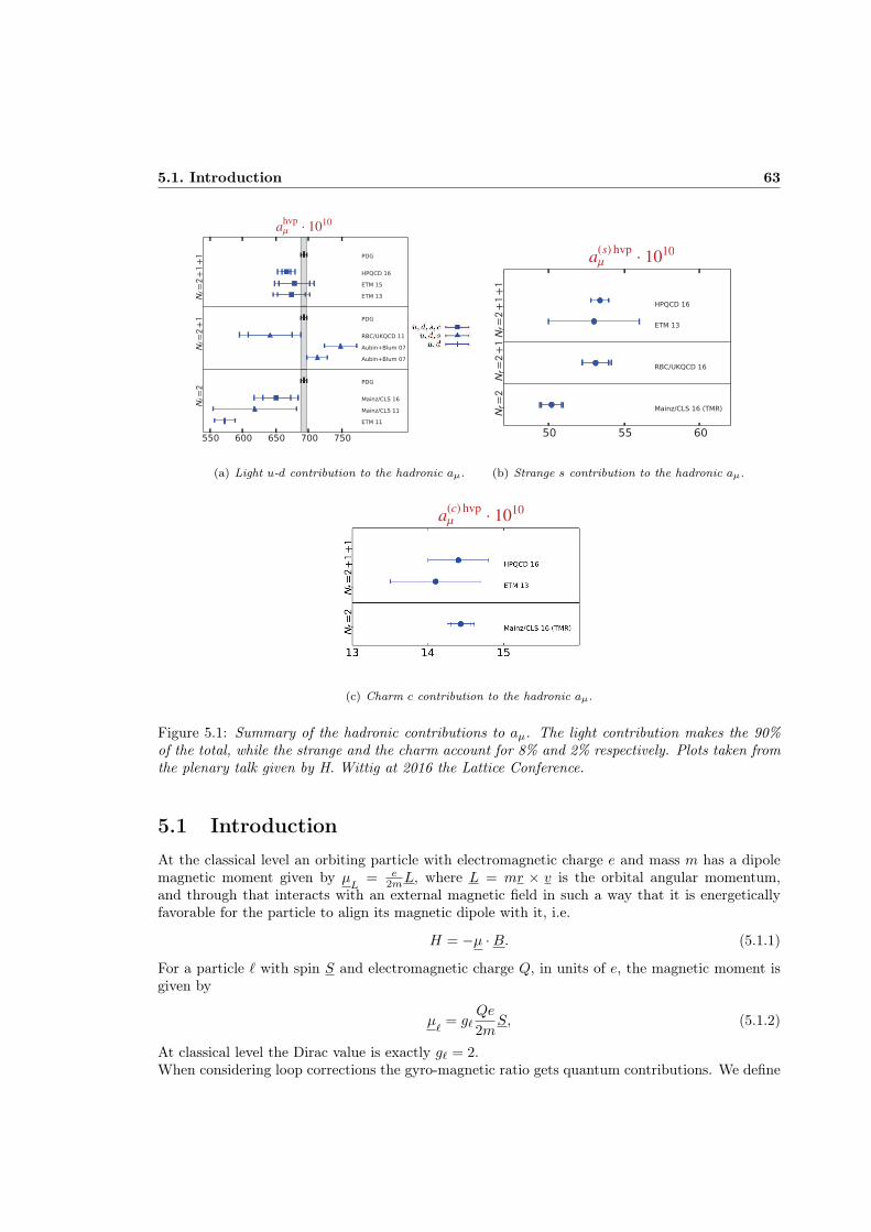
5.1. Introduction 63
ahvpµ · 1010
(a) Light u-d contribution to the hadronic aµ.
a(s) hvpµ · 1010
(b) Strange s contribution to the hadronic aµ.
a(c) hvpµ · 1010
VHWX:# -#;&S
I:YMLW1# #-##DS
8XMY=# I #-##*S
(c) Charm c contribution to the hadronic aµ.
Figure 5.1: Summary of the hadronic contributions to aµ. The light contribution makes the 90%of the total, while the strange and the charm account for 8% and 2% respectively. Plots taken fromthe plenary talk given by H. Wittig at 2016 the Lattice Conference.
5.1 IntroductionAt the classical level an orbiting particle with electromagnetic charge e and mass m has a dipolemagnetic moment given by µ
L= e
2mL, where L = mr × v is the orbital angular momentum,and through that interacts with an external magnetic field in such a way that it is energeticallyfavorable for the particle to align its magnetic dipole with it, i.e.
H = −µ ·B. (5.1.1)
For a particle ` with spin S and electromagnetic charge Q, in units of e, the magnetic moment isgiven by
µ`
= g`Qe
2mS, (5.1.2)
At classical level the Dirac value is exactly g` = 2.When considering loop corrections the gyro-magnetic ratio gets quantum contributions. We define
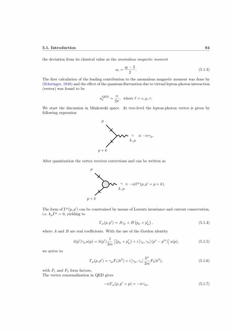
5.1. Introduction 64
the deviation from its classical value as the anomalous magnetic moment
a` =g` − 2
2. (5.1.3)
The first calculation of the leading contribution to the anomalous magnetic moment was done by(Schwinger, 1948) and the effect of the quantum fluctuation due to virtual lepton-photon interaction(vertex) was found to be
aQED` =
α
2π, where ` = e, µ, τ.
We start the discussion in Minkowski space. At tree-level the lepton-photon vertex is given byfollowing expression
γ
k, µ
p
p+ k
≡ −ieγµ.
After quantization the vertex receives corrections and can be written as
γ
k, µ
p
p+ k
≡ −ieΓµ(p, p′ = p+ k).
The form of Γµ(p, p′) can be constrained by means of Lorentz invariance and current conservation,i.e. kµΓµ = 0, yielding to
Γµ(p, p′) = Aγµ +B(pµ + p′µ
), (5.1.4)
where A and B are real coefficients. With the use of the Gordon identity
u(p′)γµu(p) = u(p′)1
2m
[(pµ + p′µ
)+ i [γµ, γν ] (pν − p′ν)
]u(p), (5.1.5)
we arrive to
Γµ(p, p′) = γµF1(k2) + i [γµ, γν ]kν
2mF2(k2), (5.1.6)
with F1 and F2 form factors.The vertex renormalization in QED gives
−ieΓµ(p, p′ = p) = −ieγµ, (5.1.7)

5.2. Details on the computation of the vacuum polarization including QEDcorrections 65
from which we infer that F1(k2 = 0) = 1, i.e. the charge of the lepton in units of e, to all orders inperturbation theory.By considering a non-relativistic electron scattered by a static potential one can show that thegyromagnetic ratio is given by
g` = 2 + 2F2(k2 = 0), (5.1.8)
and at leading order in QED F2(0) = 0. This means that the gyromagnetic ratio becomes
g` = 2 + O(α)→ a` =g` − 2
2= O(α). (5.1.9)
5.2 Details on the computation of the vacuum polarizationincluding QED corrections
We turn to the actual calculation of the HVP on the lattice. We work in the electroquenchedapproximation and use dynamical QCD configurations generated by the CLS initiative with twodegenerate flavors of non-perturbatively O(a) improved Wilson fermions (Fritzsch et al., 2012).We consider QEDL and QEDM to deal with the finite-volume zero modes, see Chap. 2. We fix thegauge to the Coulomb one in QEDL. While in the massive case we fix it to Feynman.In Fig. 5.2 we report the relevant diagrams for the leading order QED corrections to the HVP(only “continuum” diagrams are shown). Notice that those diagrams are at the same order in α asthe HLbL, that is not included. A computation including QED contribution must be performedto see whether those effects increase or decrease the discrepancy between the theoretical and theexperimental muon anomaly. In this exploratory study we neglect quark-disconnected diagrams,which are flavor-symmetry and Zweig suppressed, and all diagrams involving charged sea quarks(electroquenched approx.). We would like to compare the HVP with and without electromagneticeffects. The two HVPs will be different functions of the renormalized parameters, and to havea meaningful comparison we need to consider them at the same renormalized parameters values.One way to go could be to rescale the bare values for the change in the quark mass, the strongcoupling (reflected in the change of the lattice spacing) and the electromagnetic coupling, whenconsidering the electromagnetic corrections to the HVP. We expect all those changes to be at thepercent level. For this reason we neglect the change in the lattice spacing and the change in theelectromagnetic coupling. A percent change in the mass for quite light quark masses will cause alarge change in the pion masses, since we are working with Wilson fermions1 (see Sect. 5.2.1). Wetake into account this effect by matching the charged (or neutral) pion masses in Q(C+E)D withthe pion mass in QCD as we will see in Sect. 5.2.2.In addition we make sure that the volumes and photon masses used in QEDM are such that thecorrect dispersion relation is reproduced by the energy levels extracted from the charged pionstwo-point functions.
It should be noted that the leading electromagnetic order corrections to the HVP can beextracted also in the perturbative way as in the spirit of (de Divitiis et al., 2013).
5.2.1 Critical massWe start by first calculating the effect of the QED inclusion on the critical mass. This willserve as a cross-check of our implementations of QEDL and QEDM. We add to preexistent QCD
1There is a multiplicative plus additive renormalization in the mass.

5.2. Details on the computation of the vacuum polarization including QEDcorrections 66
(a) (b) (c) Quark-disconnected diagram, flavor-symmetry and Zweig suppressed.
(d) Absent diagram due to electro-quenched approximation.
Figure 5.2: Leading order QED corrections to the HVP in the continuum theory. Squares corre-sponds to insertions of conserved current. All orders of QCD are understood when drawing thediagrams. Diagrams (a) and (b) are included in our calculation, while (c) and (d) are absent.
configurations the quenched QED configurations by forming aU(3) gauge theory with un-improvedfermions.By using lattice perturbation theory one can estimate the QED effect on the quark mass. We takehere the results given in the App. E for the QED case. We calculate the expected shift in the Aensembles with parameters given in Tab. 5.2. In particular by using the approximations given in
Run L/a β csw κ κc amπ mπL a[fm] mπ[MeV]A3 32 5.20 2.01715 0.13580 0.1360546 0.1893(6) 6.0 0.079(3)(2) 473A4 32 5.20 2.01715 0.13590 0.1360546 0.1459(6) 4.7 0.079(3)(2) 364A5 32 5.20 2.01715 0.13594 0.1360546 0.1265(8) 4.0 0.079(3)(2) 316
Table 5.2: Gauge configuration parameters and results in QCD, see Ref. (Capitani et al., 2015).
the App. E we arrive to the critical mass calculated in the two different approximations: Eq. E.48,where 1-loop QED diagrams are taken only, and Eq. E.49, where the QED tadpole is resummedto all orders.
In order to do the comparison with the simulations we need to find an operative definition ofthe critical massmc after the inclusion of QED. We consider the unphysical theory with two quarksdegenerate in mass and charge Ψ = (u, d). We use the PCAC mass to find the critical mass, sincemPCAC = Z(β, e2)
(m0 −mc(β, e
2)). The PCAC quark mass can be defined through the spatially
integrated axial Ward identity, as in Eq. 3.5.18,
mPCAC =∂0〈A−0 (p = 0, x0)P+(0)〉〈P−(p = 0, x0)P+(0)〉 , (5.2.10)

5.2. Details on the computation of the vacuum polarization including QEDcorrections 67
where we have the following definitions,
P−(x) = Ψ(x)γ51
2
(τ1 + iτ2
)Ψ(x) = u(x)γ5d(x),
P+(x) = Ψ(x)γ51
2
(τ1 − iτ2
)Ψ(x) = d(x)γ5u(x),
A−0 (x) = Ψ(x)γ0γ51
2
(τ1 + iτ2
)Ψ(x) = u(x)γ0γ5d(x). (5.2.11)
By using Eq. 5.2.10 we extract the PCAC mass for each value of mγ . At fixed photon mass wethen perform an extrapolation, guided by chiral perturbation theory, to find the critical mass.In Fig. 5.3 we show a preliminary result for the critical mass in QCD+qQEDM simulation, orQ(C+EM)D in the following. The picture emerging is quite clear, once we include QED the quarksbecome more massive, and the results are compatible with the finite-volume lattice perturbationtheory predictions.
simulations
one loop
tadpole resummation
QCD
β = 5.2, eQ = 0.2
mγ
mc
109876543210
−0.315
−0.32
−0.325
−0.33
−0.335
−0.34
−0.345
Figure 5.3: Comparison between the critical mass from lattice perturbation theory in Feynmangauge using the one-loop result Eq. E.48 (blue stars) and the tadpole resummation Eq. E.49 (greencrosses). Orange triangles represents values from lattice simulations. The QCD critical mass isshown for comparison (red line).
5.2.2 Pseudoscalar spectrumHere we give preliminary results on the masses in the pseudoscalar sector. The masses are calculatedby cosh effective mass and fitted to a constant in the plateau region. We used one point sourceper configuration. The error is given by using a jackknife procedure. We implemented the QEDL
and QEDM at the physical value of the electric charge e ' 0.3, Qu = 2/3 and Qd = −1/3. Theresults are found in Tab. 5.3. In Fig. 5.4 we show the typical effect of the massive QED inclusionand its comparison with QEDL. For such small photon masses the result is quite stable and thecomparison is made with the QCD result. It is clear from the plot that the pseudoscalar massesbecome larger, as expected since the quark masses increase. In Fig. 5.5 we show the change with

5.2. Details on the computation of the vacuum polarization including QEDcorrections 68
Run amγ mγL amπ0,0.2 amπ0,0.1 amπ− = amπ+ Ncnf
A3 0 x .2549(9) .2071(9) .2330(9) 312A3 0.1 3.2 .2556(7) .2074(8) .2337(8) 330A3 0.25 8.0 .2553(7) .2072(8) .2331(8) 330A4 0 x .2240(8) .1691(9) .1994(9) 400A4 0.1 3.2 .2252(9) .1699(9) .2005(9) 380A4 0.25 8.0 .2246(8) .1700(10) .1998(9) 380A5 0 x .2105(7) .1526(9) .1849(8) 501A5 0.1 3.2 .2114(7) .1528(9) .1856(8) 481A5 0.25 8.0 .2111(7) .1531(9) .1852(8) 481
Table 5.3: Pseudoscalar masses in Coulomb gauge QEDL (denoted with mγ = 0) and QEDM . Theresulting pion masses go from 380 MeV to 640 MeV.
QCDmγ = 5mγ = 2
mγ = 0.2mγ = 0.15mγ = 0.05
L
mπ0(0.2,−0.2)
t
meff PS
30252015105
0.32
0.3
0.28
0.26
0.24
0.22
0.2
0.18
0.16
0.14
0.12
Figure 5.4: Effective neutral pseudoscalar massesfor different photon masses and comparison withQCD and Q(C+EL)D.
mπ+ = mπ−
mπ0,0.1
mπ0,0.2
mγ = 0.1
t
meff PS
30252015105
0.28
0.26
0.24
0.22
0.2
0.18
0.16
0.14
0.12
Figure 5.5: Effective pseudoscalarmasses for mγ = 0.1 and differentcharge content.
the charge content. For such chiral masses in QCD we know that the square of the pseudoscalarmass is linear as a function of the bare PCAC mass. We found the same linearity after theinclusion of the massive QED field (for QED case see (Duncan et al., 1996)). In Fig. 5.6 we showthe neutral pseudoscalar mass as a function of the PCAC mass for mγ = 0.1. Another exampleof that is given in Fig. 5.7, where we plot the average square masses of the uu and dd states,i.e. m2
PS = 12
(m2
PS(eQ = 0.2) +m2PS(eQ = −0.1)
), versus the sum of the two different PCAC
masses, as suggested in (Duncan et al., 1996)2. This means, upon identifying eQ1 = 0.2 and
2There it is pointed out that the linear average would introduce non analytic terms in the quark masses, whilethe square averaging respect the chiral symmetry expected from the full theory.

5.2. Details on the computation of the vacuum polarization including QEDcorrections 69
eQ2 = −0.1, that we expect the following dependence:
m2PS = A(eQ1, eQ2) +mPCAC(eQ1)B(eQ1, eQ2) +mPCAC(eQ2)B(eQ2, eQ1). (5.2.12)
eQ = 0.2
eQ = −0.1
QCD
Feynman, mγ = 0.1
mPCAC
m2 PS
0.0250.020.0150.010.0050
0.070
0.060
0.050
0.040
0.030
0.020
0.010
0.000
Figure 5.6: Neutral pseudoscalar masses versusPCAC mass for different charges.
mγ = 5
mγ = 2
mγ = 0.1
QCD
Feynman
mPCAC(0.2) +mPCAC(−0.1)
m2PS
0.040.030.020.010
0.060
0.050
0.040
0.030
0.020
0.010
0.000
Figure 5.7: Square average of neutralpseudoscalar masess versus bare PCACmasess for different photon masses.
5.2.3 Finite volume and photon mass effectsWe can take into account for finite volume and photon mass effects and correct the lattice results.The relevant formulae are given in Ref. (Borsanyi and others, 2015) for QEDL, and Ref. (Endreset al., 2016) for QEDM. We report them here for completeness and remind the reader that we areusing lattice units.Since the preliminary results concern only one volume, in QEDL, we do not perform the fit butinstead we give an estimate based on the lattice results
δVm2,LOπ± = m2
π±(L, T →∞)−m2π±(L, T ) ' Q2ακmπ±(L, T )
L, (5.2.13)
with κ = 2.837297(1). Results are given in Tab. 5.4 and we can conclude that finite volume effectsare completely negligible.
In QEDM we use the analytic formulae for the extracted masses at each volume
δVmLOπ± = 2πQ2αmγ
[I1(mγL)− 1
(mγL)3
],
δVmNLOπ± = πQ2α
m2γ
mπ±
[2I1/2(mγL) + I3/2(mγL)
], (5.2.14)
where In(z) is defined as
In(z) =1
2n+1/2π3/2Γ(n)
∑
ν 6=0
K3/2−n(z|ν|)(z|ν|)3/2−n , (5.2.15)

5.2. Details on the computation of the vacuum polarization including QEDcorrections 70
Run m2π± δVm
2,LOπ±
A3 0.0537(4) 0.00015(1)
A4 .0398(4) 0.00013(1)
A5 .0342(3) 0.00012(1)
Table 5.4: QEDL leading order finite volume corrections.
with ν ∈ Z3 and Kn modified Bessel function of the second kind. At leading order we obtain thefollowing corrections
δVmLOπ± (mγ = 0.1) = −.000097(1),
δVmLOπ± (mγ = 0.25) = −.000023(1), (5.2.16)
that are negligible at this stage. For completeness next-to-leading order results are given in Tab. 5.5.After we have corrected for the finite volume effects we need to remove the photon mass ones. Here
Run mγ mπ± δVmNLOπ±
A3 0.1 .2337(8) .000022(1)A3 0.25 .2331(8) 3.7(1) ×10−7
A4 0.1 .2005(9) .000026(1)A4 0.25 .1998(9) 4.3(1) ×10−7
A5 0.1 .1856(8) .000028(1)A5 0.25 .1852(8) 4.7(1) ×10−7
Table 5.5: QEDM next-to-leading order finite volume corrections.
we should consider the fit at next-to-leading order but since we have only two masses we use theformula at leading order, given by
δmLOπ± = mπ±(mγ →∞)−mπ±(mγ) = −α
2Q2mγ . (5.2.17)
The results are the following
δmLOπ± (mγ = 0.1) = .00036(1),
δmLOπ± (mγ = 0.25) = .00091(1), (5.2.18)
we can conclude that photon mass effects are also negligible.
5.2.4 Massless limit in QEDM
It was pointed out in Ref. (Patella, 2017) that in the limit of small photon mass the effective energyhas a linear t behavior and furthermore is constant as we change the momentum p. Here we look
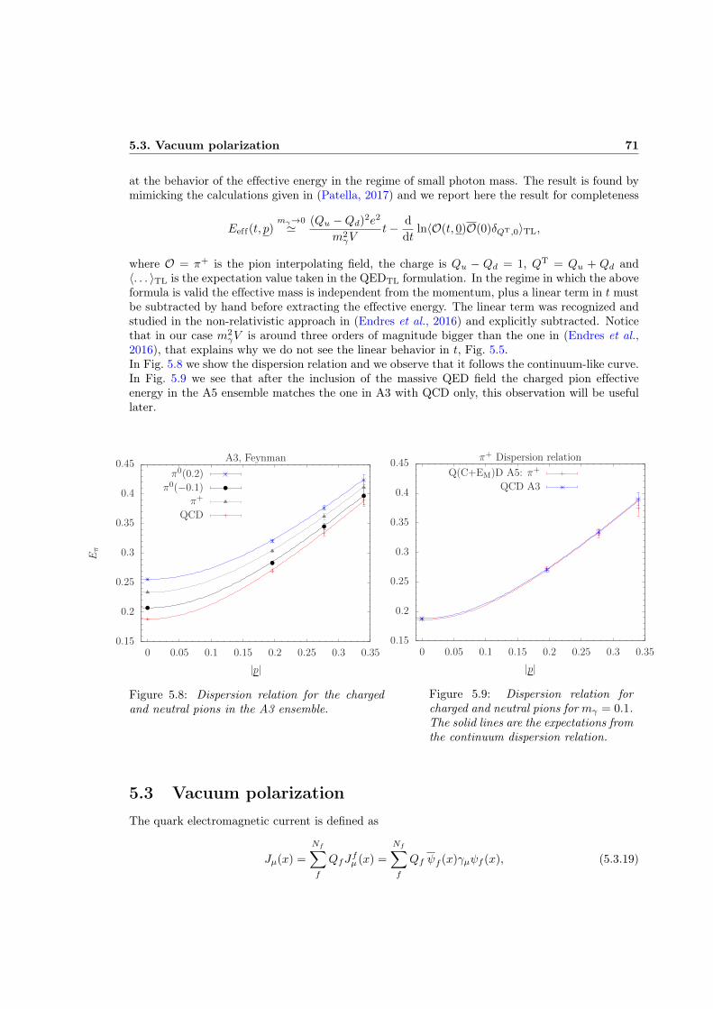
5.3. Vacuum polarization 71
at the behavior of the effective energy in the regime of small photon mass. The result is found bymimicking the calculations given in (Patella, 2017) and we report here the result for completeness
Eeff(t, p)mγ→0' (Qu −Qd)2e2
m2γV
t− ddt
ln〈O(t, 0)O(0)δQT,0〉TL,
where O = π+ is the pion interpolating field, the charge is Qu − Qd = 1, QT = Qu + Qd and〈. . . 〉TL is the expectation value taken in the QEDTL formulation. In the regime in which the aboveformula is valid the effective mass is independent from the momentum, plus a linear term in t mustbe subtracted by hand before extracting the effective energy. The linear term was recognized andstudied in the non-relativistic approach in (Endres et al., 2016) and explicitly subtracted. Noticethat in our case m2
γV is around three orders of magnitude bigger than the one in (Endres et al.,2016), that explains why we do not see the linear behavior in t, Fig. 5.5.In Fig. 5.8 we show the dispersion relation and we observe that it follows the continuum-like curve.In Fig. 5.9 we see that after the inclusion of the massive QED field the charged pion effectiveenergy in the A5 ensemble matches the one in A3 with QCD only, this observation will be usefullater.
QCD
π+π0(−0.1)
π0(0.2)
A3, Feynman
|p|
Eπ
0.350.30.250.20.150.10.050
0.45
0.4
0.35
0.3
0.25
0.2
0.15
Figure 5.8: Dispersion relation for the chargedand neutral pions in the A3 ensemble.
QCD A3
Q(C+EM)D A5: π+π+ Dispersion relation
|p|0.350.30.250.20.150.10.050
0.45
0.4
0.35
0.3
0.25
0.2
0.15
Figure 5.9: Dispersion relation forcharged and neutral pions for mγ = 0.1.The solid lines are the expectations fromthe continuum dispersion relation.
5.3 Vacuum polarizationThe quark electromagnetic current is defined as
Jµ(x) =
Nf∑
f
QfJfµ (x) =
Nf∑
f
Qf ψf (x)γµψf (x), (5.3.19)
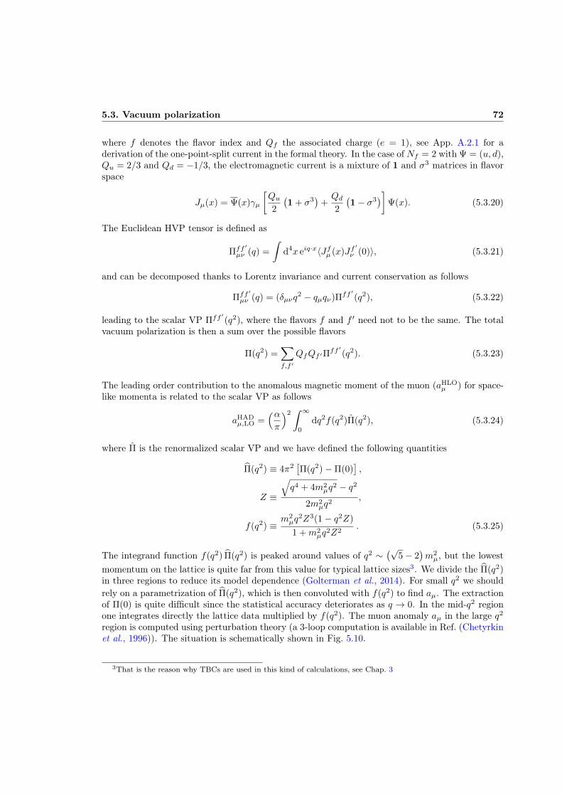
5.3. Vacuum polarization 72
where f denotes the flavor index and Qf the associated charge (e = 1), see App. A.2.1 for aderivation of the one-point-split current in the formal theory. In the case of Nf = 2 with Ψ = (u, d),Qu = 2/3 and Qd = −1/3, the electromagnetic current is a mixture of 1 and σ3 matrices in flavorspace
Jµ(x) = Ψ(x)γµ
[Qu2
(1 + σ3
)+Qd2
(1− σ3
)]Ψ(x). (5.3.20)
The Euclidean HVP tensor is defined as
Πff ′
µν (q) =
∫d4x eiq·x〈Jfµ (x)Jf
′
ν (0)〉, (5.3.21)
and can be decomposed thanks to Lorentz invariance and current conservation as follows
Πff ′
µν (q) = (δµνq2 − qµqν)Πff ′(q2), (5.3.22)
leading to the scalar VP Πff ′(q2), where the flavors f and f ′ need not to be the same. The totalvacuum polarization is then a sum over the possible flavors
Π(q2) =∑
f,f ′
QfQf ′Πff ′(q2). (5.3.23)
The leading order contribution to the anomalous magnetic moment of the muon (aHLOµ ) for space-
like momenta is related to the scalar VP as follows
aHADµ,LO =
(απ
)2∫ ∞
0
dq2f(q2)Π(q2), (5.3.24)
where Π is the renormalized scalar VP and we have defined the following quantities
Π(q2) ≡ 4π2[Π(q2)−Π(0)
],
Z ≡
√q4 + 4m2
µq2 − q2
2m2µq
2,
f(q2) ≡ m2µq
2Z3(1− q2Z)
1 +m2µq
2Z2. (5.3.25)
The integrand function f(q2) Π(q2) is peaked around values of q2 ∼(√
5− 2)m2µ, but the lowest
momentum on the lattice is quite far from this value for typical lattice sizes3. We divide the Π(q2)in three regions to reduce its model dependence (Golterman et al., 2014). For small q2 we shouldrely on a parametrization of Π(q2), which is then convoluted with f(q2) to find aµ. The extractionof Π(0) is quite difficult since the statistical accuracy deteriorates as q → 0. In the mid-q2 regionone integrates directly the lattice data multiplied by f(q2). The muon anomaly aµ in the large q2
region is computed using perturbation theory (a 3-loop computation is available in Ref. (Chetyrkinet al., 1996)). The situation is schematically shown in Fig. 5.10.
3That is the reason why TBCs are used in this kind of calculations, see Chap. 3

5.3. Vacuum polarization 73
q2
Π
Theory
Perturbation
Numerical Integration
Model
Figure 5.10: Schematic representation of the subtracted scalar Hadronic Vacuum Polarization. Inthe low q2 region, “Model”, we use for example Padé fit to estimate the HVP and we integrate theresult. In the mid-q2 region we numerically integrate directly the lattice data. In the large q2 regionwe use perturbation theory.
5.3.1 Lattice regularizationWe build the electromagnetic current in Q(C+E)D as the Noether current of the infinitesimal U(1)vector transformation
δV ψf (x) = iα(x)Qfψf (x),
δV ψf (x) = −iα(x)ψf (x)Qf . (5.3.26)
On the lattice we implement the one-point-split current, which is the conserved current of theUV(1)4 , and given as
V fµ (x) =1
2
[ψf (x)Uµ(x)(γµ − r)ψf (x+ µ) + ψf (x+ µ)U†µ(x)(γµ + r)ψf (x)
], (5.3.27)
in the case of Wilson fermions5 with r parameter of the Wilson term, see App. A.2.2 for thederivation of the current. The VP tensor is found to be
Πµν(x) =
⟨Nf∑
f
QfVfµ (x)
Nf∑
f ′
Qf ′Vf ′
µ (0)
⟩
(5.3.28)
4For Nf = 2 Eq. 2.1.7 modifies as HQ(C+E)D(Nf = 2) = U′(1)V ⊗U(1)V, where U′(1)V is the subgroup ofSU(2)V generated by σ3.
5For both the improved and un-improved theory.

5.3. Vacuum polarization 74
and by Fourier transforming the above expression we get
Πµν(q) =∑
n∈Λ
eiq·(x+µ/2+ν/2)Πµν(n), (5.3.29)
where we recall qµ ∈ Λ and qµ = 2 sin(qµ/2).When considering the diagonal term, µ = ν, we need to take into account contact terms thatmodify the expression we have given in the formal theory6. The contact term is given by
Jf,ctµ (x) =1
2
[ψf (x)Uµ(x)(r − γµ)ψf (x+ µ) + ψf (x+ µ)U†µ(x)(γµ + r)ψf (x)
],
Πf,ctµν (q) = −δµν〈Jf,ctµ (0)〉. (5.3.30)
The HVP is now given by Eqs. 5.3.30, 5.3.29, namely
Πff ′
µν (q) =
[∑
x∈Λ
eiq·(x+µ/2+ν/2)〈V fµ (x)V f′
ν (0)〉]− δµνδff ′〈Jf,ctµ (0)〉, (5.3.31)
which fulfills the WTI
qµΠff ′
µν = 0 = qνΠff ′
µν . (5.3.32)
For the explicit form of the HVP after Wick contractions see App. F.We relate the HVP to the scalar VP by using the continuum relation
Πff ′
µν (q) =(δµν q
2 − qµqν)
Πff ′(q2) + O(q4). (5.3.33)
The term O(q4)denotes all the higher order terms invariant under hypercubic transformations.
Those vanish in the continuum limit and in an anisotropic finite volume, e.g. L 6= T , the hypercubicinvariance is further broken.The scalar VP has order a effects since the conserved vector current is not improved. One way toimprove the current would be to consider the following modification
V imprµ (q) = Vµ(q) + c sin(qν/2)
∑
n
eiq·xTµν(x), (5.3.34)
where Tµν(x) = ψ(x)σµνψ(x) and c is a constant to be fitted to remove the order a effects foron-shell improvement of the matrix elements of the current V . See Ref. (Gockeler et al., 2004) forWilson fermions in the qQCD case.
5.3.2 Scalar vacuum polarizationIn order to extract the scalar VP we have to analyze the relation Eq. 5.3.33.
Off diagonal components For µ 6= ν the equation becomes
Πff ′
µν (q) = −qµqνΠff ′(q2), (5.3.35)
6Contact terms arise from the overlapping of composite operators.

5.3. Vacuum polarization 75
and by summing over all the possible N permutations of the indexes with µ 6= ν and the same q2
we obtain
Πff ′(q2) = − 1
qµqνΠff ′
µν (q) =⇒∑
µ6=νΠff ′(q2) = N Πff ′(q2) = −
∑
µ6=ν
1
qµqνΠff ′
µν (q), (5.3.36)
from which we extract the scalar VP,
Πff ′(q2) = − 1
N
∑
µ6=ν
Πff ′
µν (q)
qµqν. (5.3.37)
Diagonal components For the diagonal component µ = ν the Eq. 5.3.33 becomes
Πff ′
µµ (q) =(q2 − q2
µ
)Πff ′(q2), (5.3.38)
and again by summing over µ we find the equation for the extraction of the scalar vacuum polar-ization
∑
µ
Πff ′
µµ (q) =∑
µ
(q2 − q2
µ
)Πff ′(q2) =
(4q2 −
∑
µ
q2µ
︸ ︷︷ ︸q2
)Πff ′(q2) = 3q2Πff ′(q2), (5.3.39)
that is given by
Πff ′(q2) =1
3q2
∑
µ
Πff ′
µµ (q). (5.3.40)
Tensor zero mode subtractionIn this work we use a modified version of the HVP tensor, in particular we subtract the zero modecontribution (ZMS) from it
ΠZMSµν (q) =
∑
n∈Λ
eiq·(n+µ/2+ν/2)Πµν(n)−∑
n∈Λ
Πµν(n) = Πµν(q)−Πµν(q = 0). (5.3.41)
It has been shown in (Bernecker and Meyer, 2011) that in the infinite volume limit, thanks toLorentz symmetry, the zero mode contribution vanishes whereas in the finite volume it is notconstrained and can differ from zero. By using the ZMS version improvements in the signal-to-noise in the low q2 region can be seen, see for example Ref. (Blum and others, 2016).
5.3.3 Padé fitsSince the integrand in Eq. 5.3.24 is strongly peaked around the muon mass we need a good de-scription of the scalar VP in low q2 region. Furthermore what enters in the integral for the muonanomaly is the subtracted VP, meaning that we need to extrapolate the value Π(q2 = 0). To doso we need to parametrize the VP as a function of q2.It is known that the Taylor expansion of the VP does not converge and yields to very poor fits interms of χ2. The Padé expansion effectively increases the radius of convergence of the sum. Wecan recast the Padé fits in the following form
Rmn(q2) = Π(0) + q2
(δmnc+
m−1∑
i=0
aibi + q2
),
where n = m,m+ 1 and Π(0), ai’s and bi’s are the parameters to be fitted.

5.4. Time moments 76
5.4 Time momentsAnother way to extract the scalar VP at zero momentum involves time moments. Those givederivatives of the scalar VP with respect to q2 at zero (Chakraborty et al., 2016). We start fromEq. 5.3.33 and we consider only the diagonal spatial components µ = ν = j
Πff ′
jj (q) =(q2 − qj
)Πff ′(q2). (5.4.42)
If we restrict to momenta of the kind q = (q0, 0) and we sum over j we obtain∑
j
Πff ′
jj (q0) = 3q20Πff ′(q2
0).
The scalar VP is then given by
q20Πff ′(q2
0) =1
3
∑
j
Πff ′
jj (q0) =1
3
∑
j
∑
x0,x∈Λ
eiq0x0〈V fj (n)V f′
j (0)〉
− δff ′〈Jf,ctj (0)〉
(5.4.43)
5.4.1 Infinite volumeIn order to obtain the time moments relations we consider derivatives with respect to q0 evaluatedat zero7,
∂2k
∂q2k0
(q20Πff ′(q2
0)) ∣∣∣∣
q0=0
=1
3
∑
j,x0,x
〈V fj (x)V f′
j (0)〉(∂2k
∂q2k0
eiq0x0
) ∣∣∣∣q0=0
=1
3
∑
j,x0,x
〈V fj (x)V f′
j (0)〉 (i)2kx2k0 eiq0x0
∣∣∣∣q0=0
=1
3
∑
j,x0,x
(−)kx2k0 〈V fj (x)V f
′
j (0)〉 ≡ Gff′
2k . (5.4.44)
We have an infinite tower of relations from which we can build the Taylor expansion of the scalarVP
Πff ′(q20) =
∞∑
k=1
Gff′
2k
q2k−2
(2k)!=
1
3
∑
j,x0,x
〈V fj (x)V f′
j (0)〉∞∑
k=0
(−)kx2k0
q2k−2
(2k)!. (5.4.45)
Notice that for k = 1 in the above formula we obtain
Πff ′(q20 = 0) =
1
2
∂2
∂q20
(q20Πff ′(q2
0)) ∣∣∣∣
q0=0
= −1
6
∑
j
∑
x0,x
x20〈V fj (x)V f
′
j (0)〉 , (5.4.46)
for any parametrization of Π(q20), used to estimate Π(0) for the subtracted scalar VP.
7The contact term does not contribute since it is a constant.

5.5. Subtracted scalar HVP 77
5.4.2 Finite volumeOn the lattice we are forced to work with finite volumes, meaning that momenta are quantizedand derivatives have to be replaced by finite differences.We use the symmetric derivative definition because the error is proportional to h2, with h beingthe separation between adjacent momenta
∆f(q0)
∆q0=
1
2
(T
2π
)[f
(q0 +
2π
T
)− f
(q0 −
2π
T
)],
∆2f(q0)
∆q20
=1
22
(T
2π
)2 [f
(q0 +
4π
T
)− 2f(q0) + f
(q0 −
4π
T
)],
...
∆2nf(q0)
∆q2n0
=1
22n
(T
2π
)2n n∑
k=0
(−)k(n
k
)f
[q0 + (n− 2k)
2π
T
]. (5.4.47)
By applying the above formulae to the expression of the scalar VP in Eq. 5.4.43 we have to evaluatethe finite difference of the exponential
∆eiq0x0
∆q0
∣∣∣∣q0=0
=1
2
(T
2π
)eiq0x0
[ei2πx0/T − e−i2πx0/T
] ∣∣∣∣q0=0
=T
2πeiq0x0 i sin
(2π
Tx0
) ∣∣∣∣q0=0
=T
2πi sin
(2π
Tx0
),
∆2eiq0x0
∆q20
∣∣∣∣q0=0
=
(T
2π
)2
i2 sin2
(2π
Tx0
),
...
∆2neiq0x0
∆q2n0
∣∣∣∣q0=0
=
(T
2π
)2n
(−)n sin2n
(2π
Tx0
). (5.4.48)
By combining all the results the master formula for the time moments is given by
∆2k
∆q2k0
q20Πff ′(q2
0)
∣∣∣∣q0=0
=1
3
∑
j,x0,x
(T
2π
)2k
(−)k sin2k
(2π
Tx0
)〈V fj (x)V f
′
j (0)〉. (5.4.49)
Now we can give a specific Padé approximation of Πff ′(q20), put it in the l.h.s. of the above
formula and determine the parameters by equating the results with the r.h.s. of Eq. 5.4.49. Givena representation of the scalar VP with N parameters we need the same number of equations(given by the master formula). Then we solve the highly non-linear system in order to extract therelevant parameters. By increasing the number of parameters we are forced to increase the numberof derivatives to take into account and therefore the number of momenta to consider, see Eq. 5.4.47.This affects the estimate of an extremely local, in Fourier space, quantity as Πff ′(q2 = 0).
5.5 Subtracted scalar HVPIn this section we collect the main results for the subtracted scalar HVP. In Fig. 5.11(a) we show theresults in the case of QCD, while in Fig. 5.11(b) the unsubtracted HVP with inclusion of massive

5.6. Conclusions 78
and massless QED. Notice that Π versus r20 q
2 is a renormalized plot. The value of the Sommerparameter r0/a is calculated starting from gluonic observables that do not get electromagneticcontributions in qQED. We therefore use the values of r0/a computed in QCD, those can be foundin Ref. (Fritzsch et al., 2012).
The shape of the scalar VP is qualitatively the same with or without QED. In Fig. 5.12(a) weshow the effect of QED inclusion and the comparison is made thanks to the matching conditionpresented in Sect. 5.2. The usefulness of the matching condition is twofold; on one side it allowsfor a comparison between different ensembles, on the other side we know that the HVP is stronglydependent on the pion masses (Della Morte et al., 2012), hence we need to match the pion massesif we want to extract the EM effects.It can be seen in Fig. 5.12(c) how the QED effect is consistent with a constant within errors. Moreprecisely the effect is about 7% and compatible with zero within two/three combined sigmas. Thatsuggests to look directly at the difference of the subtracted scalar HVPs, Fig. 5.12(b). A naïveway to proceed is to model the HVPs once in QCD and once in Q(C+E)D and calculate aµ in thetwo theories. The difference encodes the QED corrections once the results have been extrapolatedto the same pion masses. This introduces large systematics due to the two fits and washes outthe QED effects. Instead we follow a different approach where we first match the pion masses andthen we model the difference for the HVPs directly. Notice this represents a one less-fit proceduredependent approach. After a good description of the difference of the HVPs is found we convolutethat with the f(q2) and get the result for aHAD,QED
µ .For a preliminary estimate of the electromagnetic effects we model the difference with Padé
fits R10 and R11 and a mixed fit, namely linear rising in q2 and then constant. By integrating thedifferent fits numerically we find
aHAD,QEDµ (R10) = (60± 28)× 10−10 ,
aHAD,QEDµ (R11) = (50± 24)× 10−10 ,
aHAD,QEDµ (mixed) = (35± 14)× 10−10 . (5.5.50)
We see that at this level the systematics, as expected, still dominate the error. One crucial thingto notice is that the electromagnetic effects go in the direction of reduce the tension betweenthe theoretical and experimental value. We checked that the conclusions do not change whenconsidering QEDL as we can see from Fig. 5.11(b). It appears that all the issues related to theQEDL formulation (Patella, 2017) are under control or do not have effect on the quantities wehave analyzed so far.
5.6 ConclusionsWe presented preliminary results for the electromagnetic effects on several observables. We dis-cussed the change in the critical mass due to the inclusion of electromagnetic interactions andcompared with perturbation theory calculations. We found the linearity of the square pseudoscalarmass in the PCAC mass. We gave results for the light pseudoscalar spectrum and we found com-pletely negligible finite volume and photon mass effect. We made sure that in QEDM we extractedthe right energy values, and that the massive approach does not reduce to a “very complicated way”to use QEDTL. For the HVP we presented a strategy to give an estimate on the electromagneticcorrections, which schematically consists in:
• matching the (charged) pion masses in different ensembles, with and without QED,
• looking directly at the difference of the subtracted HVPs in the Q(C+E)D and QCD matchedensembles.

5.6. Conclusions 79
In this way we were able to see a clear signal for the HVP that at the end reflected in an estimatefor the muon anomaly. Perhaps the most important result is that the electromagnetic correctionsin the muon anomaly clearly ameliorate the tension between theory and experiment.
The results are very encouraging and we plan to consider the inclusion of twisted boundaryconditions, in order to stabilize the fits in q2, as well as analyze different ensembles available inthe CLS initiative, in order to study the cutoff dependence, but mostly the pion mass dependenceof the EM effects.

5.6. Conclusions 80
A5
A4
A3
QCD
r20 q2
Π
20181614121086420
0.04
0.035
0.03
0.025
0.02
0.015
0.01
0.005
0
−0.005
(a) Subtracted HVP in QCD.
mγ = 0.25
mγ = 0.1
L
Q(C+E)D: A5
r20 q2
Π
20181614121086420
−0.05
−0.055
−0.06
−0.065
−0.07
−0.075
−0.08
−0.085
(b) Unsubtracted HVP in QCD + qQ(C+E)D in A5 ensemble.
Figure 5.11: HVP as a function of r0q2 with and without the inclusion of QED.

5.6. Conclusions 81
Q(C+EM)D A5: mγ = 0.25
Q(C+EM)D A5: mγ = 0.1
QCD A3
r20 q2
Π
20181614121086420
0.035
0.03
0.025
0.02
0.015
0.01
0.005
0
(a) Comparison of the scalar VP with and without QED.
mγ = 0.25
mγ = 0.1
r20 q2
ΠQ(E
+C)D(A
5)−
ΠQCD(A
3)
20181614121086420
0.0025
0.002
0.0015
0.001
0.0005
0
−0.0005
(b) Difference of the HVP with and without QED.
mγ = 0.25
mγ = 0.1
r20 q2
ΠQ(E
+C)D(A
5)−
ΠQCD(A
3)
ΠQCD(A
3)
20181614121086420
0.4
0.35
0.3
0.25
0.2
0.15
0.1
0.05
0
−0.05
−0.1
−0.15
(c) Relative difference of the QCD abd Q(C+E)D HVP.
Figure 5.12: Comparisons of the HVP on the matched ensembles.

Chapter 6
Conclusions and Outlooks
The goal of the different projects presented in this thesis was to accurately assess some residualsystematics effects in high-precision non-perturbative applications of Lattice Gauge Theories.We studied the viability of reweighting techniques for twisted boundary conditions in the spatialdirections for fermionic fields. There we suggested to compensate for the breaking of unitarity dueto the choice of different boundary conditions in the valence and sea sector. This project started inorder to estimate the above mentioned violations in the computation of renormalization factors forthe minimal walking Technicolor theory, using the RI-MOM scheme and partially twisted bound-ary conditions. We performed a complete study of the reweighting approach from tree-level toactual Monte Carlo simulations. We studied gluonic and fermionic observables in large and smallvolumes and we saw that the effect of the reweighting is at the sub-percent level. In small volumeswe found a quite pronounced sensitivity of the critical mass for un-improved Wilson fermions tochanges in the twisting angle. That is clearly a cutoff and finite volume effect that could be ratherlarge for large twisting angles.
In the second part of the thesis we presented an optimization of the HMC algorithm. No opti-mization study exists for BSM theories on the lattice. The lattice BSM field is relatively youngand the time for more precise result has come. We proposed a new strategy to find optimal pa-rameters in the case of the Omelyan integrator and Hasenbusch mass-preconditioning. The entiremethod is based on the existence of an exactly conserved quantity, the Shadow Hamiltonian. Itsimplementation is straightforward and we only needed to calculate the driving forces used duringthe Molecular Dynamics step. We implemented our strategy in the case of multi-time scales andmass-preconditioning, and we found the general form of the Shadow Hamiltonian in that case.Once the forces during the trajectory were measured we were able to give predictions on the costand acceptance of a simulation within 10% accuracy. Before that a rule of thumb was used tofind optimal parameters. The method can be also implemented on-line during the generation ofconfigurations. That is quite an appealing possibility, were the algorithm correct itself changingthe optimized parameters for the trajectories during thermalization.Since the twisted boundary conditions represent an IR regularization as a mass term, during thetime of the optimization project I also developed a twisted-boundary-preconditioning. Unfortu-nately, as we saw in the reweighting study, the pion mass becomes smaller by increasing the twistingangle. This means that there is an even worse conditioning number for the Dirac-Wilson operator,hence no speed-up was achieved. Furthermore larger forces were found, compared to the mass-preconditioning study, and the algorithm ran earlier into instabilities.
82

Chapter 6. Conclusions and Outlooks 83
In the last part of the thesis we presented a new way to isolate electromagnetic effects for thehadronic contribution to (g − 2)µ. We added quenched QED configurations to preexistent QCDones. We considered two different regularizations of the finite volume zero mode. We were ableto see a clear effect, even for physical quark charges and electromagnetic coupling. The crucialquestion to be answered in the future is whether the effect we have seen is going to be largerfor smaller pion masses or not. Within the limitations of the computation (single lattice spacing,pion mass around 400 MeV), we saw an effect of the same size as the discrepancy (in aµ) betweentheory and experiments. That is intriguing and it is clearly a motivation for continuing andimproving this study. In order to reduce the systematics, the first thing to do is to analyze morevolumes, pion masses and different lattice spacings, already available from the CLS initiative. Otherimprovements can be achieved by considering the addition of a clover term for the electromagneticpart of the action, as well as improving the vector current, in order to have better control on thecontinuum extrapolation. Another crucial effect to include in the hadronic muon anomaly in thefuture is the quark mass splitting. This effect can go in the opposite direction of the EM effects.An example of that is visible in the proton-neutron mass splitting. The reweighting techniquecan be employed to include those effects and the experience acquired in the reweighting of twistedboundary conditions can be useful.During the work on the muon anomaly we started to explore the possibility of using differentgauge conditions in order to eliminate the zero mode problem. So far in the literature no one hasconsidered the use of temporal gauge. On a lattice with periodic boundary conditions it is notpossible to fix the temporal gauge in all the sites. We need to fix two different gauges, for exampletemporal in all the sites excluding one and Coulomb gauge on the remaining. Furthermore we wouldlike to have a massive approach since it gives exponentially suppressed finite volume effects. Thatpossibility is even less clear since no simil-Stueckelberg mechanism is developed in this case. Thetemporal gauge may be particularly useful there as it would presumably remove time-dependentcorrections to the effective masses, which are due to the zero mode in A0. This is definitely a newpossibility worth to explore.


Appendix A
Ward-Takahashi Identities
A multilocal operator is given by
O(x1, x2, . . . , xn) ≡ O1(x1)O2(x2) . . .On(xn) =
n∏
k=1
Ok(xk), (A.1)
and its expectation value is formally given by the functional integral
⟨O(x1, x2, . . . , xn)
⟩=
1
Z
∫D[Aµ, ψ, ψ
]e−SYM(Aµ)−SF(A,ψ,ψ)O(x1, x2, . . . , xn) , (A.2)
where SYM is the pure gauge Yang-Mills action and SF stands for the fermionic action coupled togauge fields, see eq. 1.2.7 for the corresponding Lagrangians in QCD-like theories.As we know the functional integral is ill-defined and we need a regularization.
A.1 WTIs proofThe Ward-Takahashi identity (WTI) are found by requiring the invariance of the expectation valueunder symmetry transformations of fermionic variables. For the sake of simplicity we will omit inthe following the pure gauge action in the functional integral and in the partition function.
In order to derive the WTI we consider a generic case where G is the global symmetry groupunder investigation. The spinors transform linearly with respect the representation G(g) of thegroup, with g ∈ G, i.e.
ψ′α = Gαβ(g)ψβ . (A.3)
We consider the infinitesimal transformation as
δψα = iωataαβψβ , (A.4)
with ta hermitian and antisymmetric generators of the algebra corresponding to the symmetrygroup.
By hypothesis the action is invariant under the symmetry transformation and we suppose that
84

A.1. WTIs proof 85
also the functional measure is1
S(ψ′, ψ′) = S(ψ,ψ) ,
D[ψ′, ψ′] = D[ψ,ψ] . (A.5)
The k-th operator Ok(xk), in the multilocal, transforms as follows
δ (Ok(xk))α = iωa (Rak)αβ (Ok(xk))β (A.6)
where Rak is the representation under which the operator transforms, that can be different fromthe one of the fundamental fields.From these definitions it follows that the multilocal operator transforms as
δ (O(x1, x2, . . . , xn))α =
n∑
k=1
O1(x1) . . . δ (Ok(xk))α . . .On(xn). (A.7)
We make the transformation local, i.e. ωa ≡ ωa(x) smooth functions, and in the following weomit the matrix indexes α, β. The action will now change as follows
SF(ψ′, ψ′) = SF(ψ,ψ)− i
∫d4x (∂µω
a(x)) Jaµ(x)by p.= SF, (ψ,ψ) + i
∫d4x
(∂µJ
aµ(x)
)ωa(x) , (A.8)
where we assumed that ω is a smooth function that vanishes outside some bounded region R, andJaµ the current associated to the transformation. The operator will change as
O′(x1, x2, . . . , xn) = O(x1, x2, . . . , xn) + i
n∑
k=1
ωa(xk)O1(x1)O2(x2) . . .RakOk(xk) . . .On(xn).
(A.9)
The expectation value cannot change under the symmetry transformation, hence⟨O′(x1, . . . , xn)
⟩=⟨O(x1, . . . , xn)
⟩. (A.10)
The transformed expectation value has the form⟨O′(x1, x2, . . . , xn)
⟩=
1
Z ′∫D[ψ′, ψ′]e−SF(ψ′,ψ
′)O′(x1, x2, . . . , xn)
' 1
Z
∫D[ψ,ψ] exp
[−SF(ψ,ψ)− i
∫d4x
(∂µJaµ(x)
)ωa(x)
]
×[O(x1, x2, . . . , xn) + i
n∑
k=1
ωa(xk)O1(x1)O2(x2) . . .RakOk(xk) . . .On(xn)
],
(A.11)
and we functionally expand it with respect to the parameter δωb(y)
⟨O′⟩' 1
Z
∫D[ψ,ψ]e−SF(ψ,ψ)
(1− i
∫d4x
(∂µJ
aµ(x)
) δωa(x)
δωb(y)δωb(y)
)
×[O + i
n∑
k=1
δωa(xk)
δωb(y)O1(x1)O2(x2) . . .RakOk(xk) . . .On(xn)δωb(y)
]
'⟨O⟩− iδωb(y)
⟨∂yµJ
bµ(y)O
⟩−∑
k
δ4(y − xk)⟨O1O2 . . .RbkOk . . .On
⟩. (A.12)
1We exclude anomalous symmetries.

A.2. Singlet One-point-split current 86
By taking into account that the expectation values on l.h.s. and r.h.s. are identical and that theparameter δωb(y) can be arbitrary varied we obtain that the quantity in curly brackets must vanish.After renaming variables and indexes we get
⟨∂xµJ
aµ(x)O(x1, x2, . . . , xn)
⟩=
n∑
k=1
δ4(x− xk)⟨O1(x1)O2(x2) . . .RakOk(xk) . . .On(xn)
⟩, (A.13)
which we can write in a more compact form in the simple case of one local operator
〈δSxOy〉 = δxy〈δOy〉. (A.14)
The WTI in its final form is
∂xµ⟨Jaµ(x)O(x1, x2, . . . , xn)
⟩=
n∑
k=1
δ4(x− xk)⟨O1(x1)O2(x2) . . .RakOk(xk) . . .On(xn)
⟩. (A.15)
A.2 Singlet One-point-split currentHere we derivate the WTI in the case of a vector transformation UV(1), in the formal theory andon the lattice with un-improved Wilson fermions in the Euclidean space.
A.2.1 Formal derivationBy considering Oy = 1, and recalling that δSx/δα = ∂µJµ(x), α being the parameter of thesymmetry transformation, we have
∂µ〈Jµ(x)〉 = 0. (A.16)
The vector transformation U(1)V is given by
δV ψf (x) = iα(x)Qfψf (x),
δV ψf (x) = −iα(x)ψf (x)Qf , (A.17)
and the fermionic action is
S =
∫d4xψf (x)
(/D +mf
)ψf (x). (A.18)
The variation of the action reads
δV S = i
∫d4xψf (x)Qf
[α(x)
(/D +mf
)−(/D +mf
)α(x)
]ψf (x)
= −i∫
d4xψf (x)Qfγµψf (x) (∂µα(x))
by p.= i
∫d4xα(x)∂µ
(ψf (x)Qfγµψf (x)
)≡ 0, (A.19)
that gives ∂µ〈V fµ (x)〉 = 0 with the following definition
V fµ (x) = ψf (x)Qfγµψf (x), (A.20)
which is the electromagnetic current used in Eq. 5.3.19 with the identification V fµ (x) = QfJfµ (x).

A.3. Bare PCAC relation on the lattice 87
A.2.2 Lattice derivationThe Dirac-Wilson action on the lattice is, with r = 1, is given in Eq. E.1 and its variation underinfinitesimal vector transformations on the lattice is found to be
δV SF =∑
x,µ
i
2Qf
ψf (x) [−α(x)] (γµ − 1)Uµ(x)ψf (x+ aµ) + ψf (x)(γµ − 1)Uµ(x)α(x+ aµ)ψf (x+ aµ)
− ψf (x) [−α(x)] (γµ + 1)U†µ(x− aµ)ψf (x− aµ)− ψf (x)(γµ + 1)U†µ(x− aµ)α(x− aµ)ψf (x− aµ)
=∑
µ
i
2Qf
−∑
x
α(x)ψf (x)(γµ − 1)Uµ(x)ψf (x+ aµ)
+∑
x′=x+aµ
α(x′)ψf (x′ − aµ)(γµ − 1)Uµ(x′ − aµ)ψf (x′)
+∑
x
α(x)ψf (x)(γµ + 1)U†µ(x− aµ)ψf (x− aµ)
−∑
x′=x−aµα(x′)ψf (x′ + aµ)(γµ + 1)U†µ(x′)ψf (x′)
=∑
x,µ
i
2Qfα(x)
− ψf (x)(γµ − 1)Uµ(x)ψf (x+ aµ) + ψf (x− aµ)(γµ − 1)Uµ(x− aµ)ψf (x)
− ψf (x)(γµ + 1)U†µ(x− aµ)ψf (x− aµ)− ψf (x+ aµ)(γµ + 1)U†µ(x)ψf (x)
,
(A.21)
which can be rewritten as a total divergence
δV SF = −∑
x,µ
i
2Qfα(x)∂−µ
[ψf (x)(γµ − 1)Uµ(x)ψf (x+ aµ) + ψf (x+ aµ)(γµ + 1)U†µ(x)ψf (x)
]
= −i∑
x,µ
Qfα(x)∂−µ Vfµ (x) , (A.22)
where V fµ matches the definition of the singlet one-point-split current in Eq. 5.3.27 with r = 1
A.3 Bare PCAC relation on the latticeWe give here a derivation of the bare PCAC relation on the lattice. To this end we recall theinteraction part of the Lagrangian in the case of Ψ flavor multiplet
LIF =
1
2a
∑
µ
[Ψ(x)Uµ(x)(γµ − r)Ψ(x+ aµ)−Ψ(x+ aµ)U†µ(x)(γµ + r)Ψ(x)
]. (A.23)

A.3. Bare PCAC relation on the lattice 88
The variation of the Lagrangian under Eq. 1.2.13 axial transformations is found to be
δLIF =
1
2a
∑
µ
[Ψ(x)
(iωf (x)
σf2γ5
)Uµ(x)(γµ − r)Ψ(x+ aµ)
+ Ψ(x)Uµ(x)(γµ − r)(iωf (x+ aµ)
σf2γ5
)Ψ(x+ aµ)
−Ψ(x+ aµ)(iωf (x+ aµ)
σf2γ5
)U†µ(x)(γµ + r)Ψ(x)
−Ψ(x+ aµ)U†µ(x)(γµ + r)(iωf (x)
σf2γ5
)Ψ(x)
]. (A.24)
By renaming the variables of the second and third term we obtain
δLIL =
1
2a
∑
µ
[Ψ(x)
(iωf (x)
σf2γ5
)Uµ(x)(γµ − r)Ψ(x+ aµ)
+ Ψ(x− aµ)Uµ(x− aµ)(γµ − r)(iωf (x)
σf2γ5
)Ψ(x)
−Ψ(x)(iωf (x)
σf2γ5
)U†µ(x− aµ)(γµ + r)Ψ(x− aµ)
−Ψ(x+ aµ)U†µ(x)(γµ + r)(iωf (x)
σf2γ5
)Ψ(x)
]. (A.25)
Now we use the anticommutator relation γµ, γ5 = 0 and we find
δLIF =
iωf (x)
2a
∑
µ
[Ψ(x)Uµ(x)(−γµ − r)γ5
σf2
Ψ(x+ aµ) + Ψ(x− aµ)Uµ(x− aµ)(γµ − r)γ5σf2
Ψ(x)
−Ψ(x+ aµ)U†µ(x)(γµ + r)γ5σf2
Ψ(x)−Ψ(x)U†µ(x− aµ)(−γµ + r)γ5σf2
Ψ(x− aµ)
]
≡iωf (x)[∂−µ A
fµ − χfA
], (A.26)
where we have defined the variation of the Wilson term as χfA, which cannot be cast in form of atotal divergence, and the axial current in the following way
Afµ = −1
2
[Ψ(x+ aµ)U†µ(x)γµγ5
σf2
Ψ(x) + Ψ(x)Uµ(x)γµγ5σf2
Ψ(x+ aµ)]. (A.27)
The variation is found to be
1
i
δLF
δωf (x)
∣∣∣∣ωf (x)=0
= ∂−µ Afµ(x)− χfA −Ψ(x)γ5
σf2,M0
Ψ(x). (A.28)
We arrived at the PCAC relation on the lattice between bare quantities, M0 = m01,
∂−µ 〈Afµ(x)O(y)〉 = 2m0〈P f (x)O(y)〉+ 〈χfA(x)O(y)〉. (A.29)

Appendix B
Reweighting factors and reweightedobservables
B.1 Tree-level reweighting factorsIn the following we give the Dirac-Wilson spectrum in the case of PBCs and TBCs and the analyticevaluation of the tree-level reweighting factors. The lattice spacing is fixed to one.
B.1.1 Dirac-Wilson operator and eigenvaluesWe replace the standard links using Eq. 3.1.7. In the free case (U = 1), the forward and backwardderivatives become
∇+µ (θ)ψ(x) = [Uµ(x)ψ(x+ µ)− ψ(x)] =
[eiθµ/Lµψ(x+ µ)− ψ(x)
],
∇−µ (θ)ψ(x) =[ψ(x)− U†µ(x− µ)ψ(x− µ)
]=[ψ(x)− e−iθµ/Lµψ(x− µ)
]. (B.1.1)
The Dirac-Wilson action in momentum space reads
SW (θ) =∑
k∈Λ
ψ(k)
[(m+ 4)−
3∑
µ=0
cos (kµ + θµ/Lµ)
]14×4
+ i
[3∑
µ=0
γµ sin (kµ + θµ/L)
]ψ(k). (B.1.2)
We recall that the k’s are now in the first Brillouin zone.The Dirac-Wilson eigenvalues, at fixed momentum for each color degrees of freedom, are
λ1,2 = (m+ 4)−3∑
µ=0
cos (kµ + θµ/Lµ) + i
(3∑
µ=0
sin2 (kµ + θµ/Lµ)
)1/2
,
λ3,4 = (m+ 4)−3∑
µ=0
cos (kµ + θµ/Lµ)− i(
3∑
µ=0
sin2 (kµ + θµ/Lµ)
)1/2
. (B.1.3)
In Fig. B.1 we show the effect of θµ = (0, θ) on the Dirac-Wilson spectrum.
89

B.1. Tree-level reweighting factors 90
θ = 0.5
θ = 0
Dirac Wilson spectrum, L = 4
ℜeλ
ℑmλ
876543210
3
2
1
0
−1
−2
−3
Figure B.1: Dirac-Wilson spectrum for different values of θ in V = 44 volume and mass m0 = 0.2.
B.1.2 Reweighting factors: tree-level analytic evaluationFrom the knowledge of the eigenvalues Eq. B.1.3 we write down the tree-level reweighting factorEq. 3.2.10
Wθ =∏
k∈Λ
[(m+ 4)−∑µ cos (kµ + θµ/Lµ)
]2+∑µ sin2 (kµ + θµ/Lµ)
[(m+ 4)−∑µ cos (kµ)
]2+∑µ sin2 (kµ)
2Nc
, (B.1.4)
recalling that θ0 = 0.
Small θ expansion We perform a perturbative expansion around θµ = 0. The exponential ofthe action becomes
exp (−Sθ) ' exp (−S + θµJµ) ' exp (−Sθ) (1 + θµJµ) , (B.1.5)
with a suitable current Jµ. The vacuum expectation value of an operator O becomes 〈O〉θ '〈O〉+ θµ〈OJµ〉. We know that 〈OJµ〉 ≡ 0 vanishes because of Lorentz invariance, so we concludethat any expectation value must start with a correction1 of order θ2
〈O〉θ ' 〈O〉+ O(θ2). (B.1.6)
Large m expansion We analyze the behavior of the tree-level reweighting factor in Eq. B.1.4for m→∞.
1Similar argument is made for the expansion of the observable in θ, if it depends on the twisting angle.

B.2. Observables with TBCs 91
We start by looking at the numerator
[(m+ 4)−
3∑
µ=0
cos (kµ + θµ/Lµ)
]2
+
3∑
µ=0
sin2 (kµ + θµ/Lµ)
' (m+ 4)2 − 2m
4∑
µ=1
cos (kµ + θµ/Lµ) ' m2 + 2m
(4−
3∑
µ=0
cos (kµ + θµ/Lµ)
). (B.1.7)
We build the ratio and we obtain
m2 + 2m(
4−∑3µ=0 cos (kµ + θµ/Lµ)
)
m2 + 2m(
4−∑3µ=0 cos kµ
) 'm2 + 2m
(4−∑3
µ=0 cos (kµ + θµ/Lµ))
m2[1 + 2
m
(4−∑3
µ=0 cos kµ
)]
'[
1 +2
m
(4−
3∑
µ=0
cos (kµ + θµ/Lµ)
)][1− 2
m
(4−
3∑
µ=0
cos kµ
)]
' 1 +2
m
3∑
µ=0
[cos kµ − cos (kµ + θµ/Lµ)] . (B.1.8)
The reweighting factor become
Wθ '∏
k∈Λ
1 +
2
m
3∑
µ=0
[cos kµ − cos (kµ + θµ/Lµ)]
2Nc
'∏
k∈Λ
1 +
4Ncm
3∑
µ=0
[cos kµ − cos (kµ + θµ/Lµ)]
' 1 +4Ncm
∑
k∈Λ
3∑
µ=0
[cos kµ − cos (kµ + θµ/Lµ)]
' 1 +4Ncm
∑
k∈Λ
3∑
j=1
[cos kj − cos (kj + θ/Lj)]
. (B.1.9)
Here the integral over the interval (−π, π) of the function in the curly brackets is vanishing, whichimplies that the correction in 1/m starts to the second order,
Wθ = 1 + O(m−2
). (B.1.10)
B.2 Observables with TBCsHere we give the relevant formulae for the observables, i.e. the plaquette and the pion dispersionrelation, studied in the reweighting project in Chap. 3.
B.2.1 PlaquetteThe most simple observable that we can think to reweight is the plaquette because it has nodependence on the field B = θ/L.

B.2. Observables with TBCs 92
The plaquette on the lattice is defined as the shortest loop path and is the product of links
P [U ] = Tr ∏
(x,µ)∈loop
Uµ
. (B.2.11)
In the case of constant U(1) interaction (Eq. 3.1.7) the plaquette becomes
P [U ] = Tr ∏
(x,µ)∈loop
Uµ
= Tr ∏
(x,µ)∈loop
eiBµUµ
= Tr ∏
(x,µ)∈loop
Uµ
= P [U ], (B.2.12)
because we always find two different modified links pointing in opposition direction and thereforethe constant B-term disappear.The reweighted plaquette expectation value is then
〈P [U ]〉θ = 〈P [U ]〉θ =〈P [U ]Wθ〉0〈Wθ〉0
. (B.2.13)
B.2.2 Valence twisting and pion dispersion relationWe are interested in expectation values of meson interpolators when two flavors f1, f2 are involved.The most general form for such interpolators is
OM(x) = ψ(f1)
(x)Γψ(f2)(x), OM(y) = ψ(f2)
(y)Γψ(f1)(y),
where Γ is an element of the Clifford algebra, i.e. combination of the γ matrices. The operator Ocreates a meson, with the right quantum numbers, from the vacuum and O annihilates that state.We need to compute the Grassmann integrals in order to calculate the fermionic expectation value〈. . . 〉F . We choose the two flavors to be f1 = u, f2 = d, in order to have an iso-triplet operator2.The fermionic expectation values can be computed by employing Wick contractions as follows
〈O(x)O(y)〉F =⟨(dΓu
)(x) (uΓd) (y)
⟩F
= Γα1β1Γα2β2
⟨(dα1,c1uβ1,c1
)(x)(uα2,c2dβ2,c2
)(y)⟩F
= −Γα1β1Γα2β2
⟨uβ1,c1(x)uα2,c2(y)
⟩u
⟨dβ2,c2(y)dα1,c1(x)
⟩d
= −Γα1β1Γα2β2
D−1u (y, x)β1,α2;c1,c2D
−1d (y, x)β2,α1;c2,c1
= −Tr[ΓD−1
u (x, y)ΓD−1d (y, x)
], (B.2.14)
where in the second line we explicitly showed Dirac indexes with Greek letters and color indexeswith Latin ones; in third line we used the factorization property of the fermionic expectation valuewith respect to flavor3 〈. . . 〉F = 〈. . . 〉u〈. . . 〉d and we interchanged the fermion spinors accordingto their Grassmann nature. In Fig. B.2 we draw in a diagrammatic way the result of the aboveWick contractions in the case of O = dγ5u at zero momentum, which correspond to a charged pionπ±. In order to extract the dispersion relation from the correlator we project the interpolators to
2To avoid the contribution of disconnected diagrams that suffer from the signal-to-noise problem.3The action and the partition function are separable in the flavor space, i.e. SW =
∑f ψfDWψf =
Su + Sd, ZF = ZuZd. That implies that the fermionic expectation value can be written as 〈. . . 〉F =
Z−1F∫D [u, u]D
[d, d]e−SF (. . . ) =
[Z−1u
∫D [u, u] e−Su (. . . )u
] [Z−1d
∫D[d, d]e−Sd (. . . )d
]= 〈. . . 〉u〈. . . 〉d.

B.2. Observables with TBCs 93
γ5γ5
d→
u→
(k0, p
)
(p0, p
)
π± → (p0 − k0, 0) ≡ (mπ, 0)
Figure B.2: Diagrammatic expression of the Eq. B.2.14. We show on the diagram the momentumflow.
a definite momentum, say p. The correlator has the following behaviour for large time separations(x0 1)
〈O(x0, p)O(0)〉 =1√|V |
∑
x∈V3
e−ix·p〈O(x)O(0)〉
=∑
k
〈0|O|k〉〈k|O†|0〉e−x0Ek =x01
Ae−x0E(p), (B.2.15)
where E(0) = mπ.The free dispersion relation on the lattice is obtained from the free boson lattice propagator inmomentum space (inverse of the Klein-Gordon operator on the lattice), and restoring the latticespacing a we get
cosh(aE) = cosh(amπ) +
3∑
k=1
[1− cos(apk)] −→ap→0
E2 = m2π + |p|2. (B.2.16)
In the presence of a constant U(1) interaction in the spatial direction we perform the substi-tution p → p + B. That corresponds to a twisting in the valence only. In Fig. B.3 we show thechange on the momentum flow in the diagram in the zero momentum pion case. The dispersion
γ5γ5
d→
u→
(k0, p+B
)
(p0, p
)
π± → (p0 − k0,−B) ≡ (E,−B)
Figure B.3: Diagrammatic expression of the Eq. B.2.14 in the presence of the constant U(1)interaction. The state correspond to a charged pion with momentum B.

B.2. Observables with TBCs 94
relation in this case is
cosh(aE) = cosh(amπ) +
3∑
k=1
[1− cos(apk + aBk)] −→ap→0
E2 = m2π + |p+B|2. (B.2.17)
It is clear that the charged pion momentum on the lattice becomes
pπ
= p+B =2πn+ θ
aL. (B.2.18)
Appendix C
HMC simulations
C.1 Acceptance in HMC simulationsWe follow Ref. (Gupta et al., 1990) to work out the acceptance probability.The acceptance is found from the Creutz equality, which comes from the area preserving require-ment,
〈e−∆H〉 = 1, (C.1.1)
where ∆H = Hf −Hi, and by expanding it into cumulants we get
〈∆H〉 =1
2Var(∆H) + higher cumulants. (C.1.2)
When the volume is large enough, i.e. compared with the relevant correlation length, the cumulantswill grow linearly while their dependence on the step size is different in δτ . In order to have afinite 〈∆H〉 then δτ should be varied to keep the variance fixed, Var(∆H) = const.The distribution for the acceptance will be a convolution of a Gaussian with mean and widthrelated by 〈∆H〉 = Var(∆H)/2 ≡ σ2
0/2 and an Metropolis test
Pacc(∆H) =1√
2πσ0
∫ ∞
−∞min(1, e−x) exp
[− (x− 〈∆H〉)2
2σ20
]dx
=1√
2πσ0
∫ 0
−∞exp
[− (x− 〈∆H〉)2
2σ20
]dx+
∫ ∞
0
exp
[− (x− 〈∆H〉)2
2σ20
− x]dx.
(C.1.3)
By changing the coordinates in the first integral to z = x−〈∆H〉√2σ0
we get
first integral = 2〈∆H〉1/2∫ −
√〈∆H〉2
−∞e−z
2
dz = 2〈∆H〉1/2∫ ∞√〈∆H〉2
e−z2
dz
=√π〈∆H〉1/2erfc
(√〈∆H〉2
), (C.1.4)
where we used the symmetry of the Gaussian integral in the first step.For the second integral we first recognize the square and use the relation between the variance and
95
C.2. Multiple time-scale Omelyan shadow Hamiltonian 96
the mean
(x− 〈∆H〉)2
2σ20
+ x =(x+ 〈∆H〉)2
4〈∆H〉 , (C.1.5)
and then change the variable to z = x+〈∆H〉2√〈∆H〉
, obtaining
second integral = 2〈∆H〉1/2∫ ∞√〈∆H〉2
e−z2
dz =√π〈∆H〉1/2erfc
(√〈∆H〉2
). (C.1.6)
By putting all together, with the right pre-factors, we get the formula
Pacc(∆H) = erfc
(√〈∆H〉2
). (C.1.7)
We use C.1.2 to trade 〈∆H〉 with Var(∆H) because the latter is a better behaved quantity1
Pacc(Var(∆H)) = erfc
(√Var (∆H)
8
). (C.1.8)
C.2 Multiple time-scale Omelyan shadow HamiltonianFollowing Ref. (Clark et al., 2008) we give the expression for the shadow Hamiltonian in the caseof multi-time scale.Let the Hamiltonian be
H = T +∑
i
Si , (C.2.9)
with i index running to as many multi-time scales are present.Let be expZ = expA expB, then the Baker-Campbell-Hausdorff formula is given by
Z =(A+B) + [A,B] +1
12([A, [A,B]] + [B, [B,A]])
− 1
24[B, [A, [A,B]]]− 1
720([B, [B, [B, [B,A]]]] + [A, [A, [A, [A,B]]]]) + . . . (C.2.10)
From the above formula we can evaluate the following expression
ln (exp(X) exp(Y ) exp(X)) = (2X + Y ) +1
6([[X,Y ], X] + [[X,Y ], Y ]) + . . . (C.2.11)
We use the work done in Ref. (Reinsch, 2000) in MATHEMATICA to calculate BCH and conse-quently the shadow Hamiltonian.
1In the mean 〈∆H〉 we can have negative and positive contributions and that may lead to large uncertainties.

C.2. Multiple time-scale Omelyan shadow Hamiltonian 97
One level Leap-frog integratorThe Leap-frog integrator is given by the following evolution operator
[exp
(δτ
2S
)exp
(δτ T
)exp
(δτ
2S
)]n, (C.2.12)
with δτ = 1/n, and by employing the BCH formula in Eq. C.2.11 we get(
exp
[Hδτ +
(1
12[[S, T ], T ] +
1
24[[S, T ], S]
)δτ3
])n. (C.2.13)
By applying the BCH formula again we get
H = H +
(1
12[[S, T ], T ] +
1
24[[S, T ], S]
)δτ2. (C.2.14)
One-level Omelyan integratorThe one-level Omelyan integrator is given by
[exp
(αδτS1
)exp
(δτ
2T
)exp
(δτ(1− 2α)S1
)exp
(δτ
2T
)exp
(αδτS1
)]n. (C.2.15)
The shadow Hamiltonian is found to be
H = H +
[6α2 − 6α+ 1
12[[T , S1], S1] +
6α− 1
24[[S1, T ], T ]
]δτ2. (C.2.16)
Two-level Omelyan integratorThe two-level Omelyan integrator is obtained by operating the following formal substitution to theone-level Omelyan integrator
exp
(δτ
2T
)−→
[exp
(αδτ
2mS2
)exp
(δτ
4mT
)exp
(δτ
2m(1− 2α)S2
)exp
(δτ
4mT
)exp
(αδτ
2mS2
)]m.
(C.2.17)
The shadow Hamiltonian is found to be
H =H − δτ2 6α2 − 6α+ 1
12
[[[S1, T ], S1] +
1
2m2[[S2, T ], S2]
]
+ δτ2 6α− 1
24
[[[S1, T ], T ] + +
1
2m2[[S2, T ], T ] +
1
2m2[[S2, T ], S1]
]. (C.2.18)
Multi-level Omelyan integratorBy playing the same game we can recognize a structure in the shadows Hamiltonian, which willbe given by
H = H + τ2∑
i=1
[6α2 − 6α+ 1
3
([Si, [Si, T ]]∏ij=1(2nj)2
)
+6α− 1
6
([T , [T , Si]]−
∑j<i[Sj , Si, T ]]
∏ij=1(2nj)2
)], (C.2.19)
where τ = δτ × n0 and n0, n1, . . . ni are the i number of integration steps per level.

C.3. Forces in HMC 98
C.3 Forces in HMCThe forces in HMC are derived as in Ref. (Del Debbio et al., 2010). In the following we omitthe sum over space-time, color and spin. The Hamiltonian in the HMC evolution is given byH = T + SG + SF,
• Gaussian weight for the momenta π,
T =π2
2, (C.3.20)
where π ∈ su(Nc), πµ(x) = iπaµ(x)T af , where Taf are the hermitian generators in the funda-
mental representation.
• Wilson plaquette gauge action
SG = β∑
µ<ν
(1− 1
Nc<eTrPµν
), (C.3.21)
where β = 2Nc/g2, and Pµν the plaquette in the (µ, ν) plane
Pµν = Uµ(x)Uν(x+ µ)U†µ(x+ ν)U†ν (x). (C.3.22)
• Fermionic action
SF = φ†(Q2)−1
φ, (C.3.23)
where φ is a pseudofermion, Q = γ5Dm is the γ5 Dirac-Wilson operator, DW that is givenby the following equation
DWψ(x) = 8ψ(x)− 1
2
∑
µ
[(1− γµ)URµ (x)ψ(x+ µ) + (1 + γµ)UR,†µ (x− µ)ψ(x− µ)
]
(C.3.24)
Dmψ(x) = (DW +m0)ψ(x). (C.3.25)
The URµ are the link variables in the representation R.
A generic element x in the algebra su(Nc) is written as x = ixaT af , and its norm is given by||x||2 = Tr(x†x) = Tf
∑i,j |xij |2. Tf is the normalization of the generators in the fundamental
representation, for other representation we write TR.
Equation of motionThe equation of motion for the links is found by taking the derivative with respect to τ (the Markovtime) of 1 = Uµ(τ)U†µ(τ)
Uµ(τ)U†µ(τ) + Uµ(τ)U†µ(τ) = 0. (C.3.26)
The equation is fulfilled by taking
Uµ(x) = πµ(x)Uµ(x). (C.3.27)

C.3. Forces in HMC 99
The equation of motion for the momenta can be obtained by requiring that the Hamiltonian H isa conserved quantity
H = 0 = T + SG + SF. (C.3.28)
For the first two derivatives we have
T = Tf∑
x,µ,a
πaµ(x)πaµ(x) , (C.3.29)
SG = − β
Nc
∑
x,µ
<eTr[Uµ(x)V †µ (x)
]
= − β
Nc
∑
x,µ
<eTr[πµ(x)Uµ(x)V †µ (x)
]
= − β
Nc
∑
x,µ,a
πaµ(x)<eTr[iT af Uµ(x)V †µ (x)
], (C.3.30)
where Vµ(x) is sum of the staples around the link Uµ(x).For the fermionic force we write
SF = −φ†(Q2)−1 ˙(Q2)
(Q2)−1
φ , (C.3.31)
and we define η =(Q2)−1
φ and ξ = Qη.By using the hermiticity of Q2 we rewrite the derivative as
SF = −2ξ†Q η. (C.3.32)
Inserting the explicit form of Q = γ5DW we get
SF = <e∑
x,µ
ξ†(x)URµ (x)γ5(1− γµ)η(x+ µ)
+ η†(x)UR,†µ (x)γ5(1− γµ)ξ(x+ µ). (C.3.33)
By collecting the results we get the equation of motion for the momenta
πaµ(x) = πa,Gµ (x) + πa,Fµ (x), (C.3.34)
πa,Gµ (x) =β
Nc
1
Tf<eTr
[iT af Uµ(x)V †µ (x)
]≡ F aµG (x), (C.3.35)
πa,Fµ (x) =− 1
Tf<eTr
iT aRU
Rµ (x)γ5(1− γµ)
[η(x+ µ)⊗ ξ†(x) + ξ(x+ µ)⊗ η†(x)
]≡ F aµF (x).
(C.3.36)
Where we denoted as F the associated driving forces to the different part of the action.
C.3.1 Mass preconditioning forcesThe mass preconditioning is given in Eq. 4.2.23. The QHMC part follows exactly as before but witha shift in the mass given by m0 + µ. We derive here the force associated to the Hasenbusch term.We write the associated action as, with φ2 different set of pseudofermions,
SHase = φ†2Q−1(D†m + µ
)(Dm + µ)Q−1φ2. (C.3.37)

C.3. Forces in HMC 100
The operator can be rewritten as follows
Q−1(D†m + µ
)(Dm + µ)Q−1 = D−1
m γ5 (γ5Dmγ5 + µ) (Dm + µ)D−1m γ5
=(γ5 + µD−1
m γ5
) (γ5 + µD−1
m γ5
)
=(γ5 + µQ−1
) (γ5 + µQ−1
), (C.3.38)
and the action becomes
SHase = φ†2(γ5 + µQ−1
) (γ5 + µQ−1
)φ2. (C.3.39)
Now we take the derivative with respect to the Markov time
SHase = φ†2
[µ ˙(Q−1)
(γ5 + µQ−1
)+ µ
(γ5 + µQ−1
) ˙(Q−1)]φ2
= −µφ†2[Q−1QQ−1
(γ5 + µQ−1
)+(γ5 + µQ−1
)Q−1QQ−1
]φ2. (C.3.40)
Note that the above equation has the standard form of a fermionic force in the HMC algorithmprovided that
X ≡ Q−1φ2,
Y ≡ Q−1(γ5 + µQ−1
)φ2, (C.3.41)
in particular, see Eq. C.3.32,
SHase = −2µX†QY. (C.3.42)
The forces given by the different pieces of the action are
F aµG (x) =β
Nc
1
Tf<eTr
[iT af Uµ(x)V †µ (x)
], (C.3.43)
F aµHMC(x) =− 1
Tf<eTr
iT aRU
Rµ (x)γ5(1− γµ)
[η(x+ µ)⊗ ξ†(x) + ξ(x+ µ)⊗ η†(x)
], (C.3.44)
F aµHase(x) =− µ
Tf<eTr
iT aRU
Rµ (x)γ5(1− γµ)
[Y (x+ µ)⊗X†(x) +X(x+ µ)⊗ Y †(x)
],
(C.3.45)
where
ξ ≡ Q−1φ1, (C.3.46)
η ≡(Q2)−1
φ1, (C.3.47)
X ≡ Q−1φ2, (C.3.48)
Y ≡ Q−1(γ5 + µQ−1
)φ2, (C.3.49)
and we recall that Q in this case is the mass shifted γ5 Dirac-Wilson operator
Q = γ5(Dm + µ) = γ5(DW +m0 + µ). (C.3.50)

C.4. Number of configurations and parameters in the optimization study 101
C.4 Number of configurations and parameters in the opti-mization study
Here we collect the number of configurations analyzed in the force study in Chap. 4. Simulationscorrespond to a SU(2) gauge group with a doublet of un-improved Wilson fermions in the funda-mental representation and Wilson plaquette gauge action in a V = 324 volume. The value mc ofthe bare mass parameter yielding massless fermions is estimated to be −0.77(2) at β = 2.2 (Lewiset al., 2012,Hietanen et al., 2014,Arthur et al., 2016). The integrator choice is the Omelyan withα = 1/6. The inversions of the γ5-hermitian Dirac-Wilson operator are performed using a versionof the Quasi-Minimal Residual (QMR). The algorithm is not absolutely convergent and in the caseof no convergence our implementation switch to the BiCGstab algorithm. For the evolution of thegauge field we use the Minimal Residual Extrapolation (MRE) algorithm to build an initial guessfor the inverter based on the past solutions (Brower et al., 1997). In particular 5 past solutionswhere stored throughout the HMC simulation. The force precision was set to 10−14 and the ∆Hmeasurement precision for the accept-reject step to 10−14, which is enough to ensure reversibility ofthe algorithm. The level parameters are n for the Hasenbusch, m HMC and k Gauge as describedin Sect. 4.2.
m0 = −0.72
n = 15, m = 8, k = 10.
µ Ncnf
0.05 1090.1 980.15 1280.2 1530.25 1280.3 1360.35 1440.4 1550.45 1120.5 115
µ Ncnf
0.6 1240.7 1300.75 1330.8 690.9 1371 11931.5 802 14872.5 883 92
m0 = −0.735
n = 5, m = 4, k = 10.
µ Ncnf
0.05 1330.1 1890.15 202
µ Ncnf
0.2 2020.25 2020.3 2020.35 202

C.4. Number of configurations and parameters in the optimization study 102
m0 = −0.75
n = 15, m = 8, k = 10.
µ Ncnf
0.05 570.1 790.15 1190.2 1470.25 152
µ Ncnf
0.3 1780.35 1780.4 1960.45 1860.5 2010.6 193

Appendix D
Quantum electrodynamics on thelattice: supplementary material
D.1 Fourier transformWe set the notation for the Fourier transform on the lattice. The reciprocal lattice Λ, with periodicboundary conditions for a functions f(n+ µLµ) = f(n) ∀µ, is given by
Λ =
p = (p0, p1, p2, p3) : pµ =
2π
aLµkµ, with kµ ∈
(−Lµ
2,Lµ2
]⊂ Z
.
The delta functions are defined as
δ(x− x′) =1
V
∑
p∈Λ
exp (ip · (x− x′)) ,
δ(p− p′) =1
V
∑
n∈Λ
exp (i(p− p′) · x) . (D.1.1)
The Fourier transform and the inverse are defined as
f(p) =1√V
∑
n∈Λ
exp (−ip · x) f(x),
f(x) =1√V
∑
p∈Λ
exp (ip · x) f(p). (D.1.2)
D.1.1 Reality conditionLet us consider the Fourier transform of a real quantity such as the electromagnetic field, Aµ(x+
aµ/2). This will add some conditions on the Fourier coefficients Aµ(p) (Blum et al., 2007).The Fourier transform of the gauge field is
Aµ(x+ aµ/2) =1√V
∑
p∈Λ
eip·(x+aµ/2)Aµ(p), (D.1.3)
103

D.2. Generation in Feynman gauge 104
and the reality condition means that the imaginary part of the Fourier transform has to vanish,i.e.
1√V
∑
p∈Λ
sin (p · x+ apµ/2)<eAµ(p) + cos (p · x+ apµ/2)=mAµ(p)
= 0. (D.1.4)
We introduce the reflection operator in the first Brillouin zone
R(p)µ =
−pµ if pµ 6= π
π if pµ = π. (D.1.5)
We can now write the reality condition into three different ones:
1. pµ = 0, the zero mode is real, =mAµ(0) = 0.
2. pµ 6= 0, π, there is a pairwise cancellation between one mode and the reflected-conjugate one,i.e.
Aµ(p) = A∗µ (R(p))←→<eAµ(p) = <eAµ(R(p))
=mAµ(p) = −=mAµ(R(p)).
3. pµ = π, pν = 0, π for ν 6= µ, there is no partner for these kind of modes, which means nopairwise cancellation and =mAµ(p) = 0. While the real part is left unfixed since the sine inEq. D.1.4 is vanishing.
We can incorporate these conditions in one, which reads
eiR(p)µ/2Aµ (R(p)) =(eipµ/2Aµ(p)
)∗. (D.1.6)
D.2 Generation in Feynman gaugeWe recall that the action in Feynman gauge in coordinate space is
S = −1
2
∑
n∈Λ
∑
µ,ν
Aν(x+ aν/2)∂−µ ∂+µ Aν(x+ aν/2). (D.2.7)
To find the action in the momentum space we Fourier transform by inserting Eq. D.1.3
S = − 1
2V
∑
n∈Λ
∑
µ,ν
∑
p,p′∈Λ
eip·(x+aν/2)∂−µ ∂+µ e
ip′·(x+aν/2)A(p)A(p′). (D.2.8)
The Laplacian of the exponential is found to be
∂+µ e
ip′·x =eip′·x
a
(eip′µ − 1
),
∂−µ ∂+µ e
ip′·x =eip′·x
a2
(1− e−ip
′µ
)(eip′µ − 1
)=[2i sin(p′µ/2)
]2 ≡ −p′2µ ,∑
µ
∂−µ ∂+µ e
ip′·x = −∑
µ
p′2µ ≡ −p
′2 , (D.2.9)

D.3. Extended Coulomb gauge 105
and the action becomes
S =1
2V
∑
n∈Λ
∑
ν
∑
p,p′∈Λ
ei(p+p′)·(x+aν/2)p′A(p)A(p′). (D.2.10)
We recognize the the delta function, Eq. D.1.1, hence we are left with
S =1
2V
∑
ν
∑
p,p′∈Λ
V δ(p+ p′)eiapν/2e−iap′ν/2 p
′2 A(p)A(p′). (D.2.11)
The delta function in the first Brillouin zone is equivalent to the reflection operation given inEq. D.1.5
S =1
2
∑
p∈Λ
p2∑
ν
eiapν/2 A(p) e−iaR(p)ν/2 A (R(p)) , (D.2.12)
and by using the reality condition, in Eq. D.1.6 we obtain the result
S =∑
p∈Λ
p2
2
∑
ν
∣∣A(p)∣∣2. (D.2.13)
D.3 Extended Coulomb gaugeThe Coulomb gauge is defined by the constraint (see Faddeev-Popov approach in Sect. 2.3.1),
G(A) =∑
j
∂jAj , (D.3.14)
and we shall take α = 1. On the lattice the condition is translated∑
j
∂−j Aj(x+ aj/2) = 0 , A0(p0 6= 0, p = 0) = 0 , (D.3.15)
with j spatial index. The second condition is a consequence of the non-completeness of the Coulombgauge in finite volume, hence the name “extended”, see Sect. 2.4 for details.
D.3.1 Extended Coulomb via Feynman gaugeWe can generate first the Fourier component of the field in Feynman gauge and then switch toCoulomb by employing a gauge transformation
Aµ(x+ aµ/2) = ACµ (x+ aµ/2) + ∂+
µ α(x), (D.3.16)
where Aµ is the field generated in Feynman gauge, ACµ is the field we would like to satisfy the
Coulomb gauge condition and α is the gauge transformation that does the job, see Ref. (Borsanyiand others, 2015). By imposing the Coulomb gauge condition one can relate α and Aµ,
∑
j
∂−j Aj(x+ aj/2) =
∑
j
∂−j ACj (x+ aj/2) +
∑
j
∂−j ∂+j α(x). (D.3.17)

D.3. Extended Coulomb gauge 106
We Fourier transform the above relation
l.h.s. :∑
j
∂−j Aj(x+ aj/2) =∑
p∈Λ
eip·x∑
j
1− e−iapj
aeiapj/2Aj(p)
=∑
p∈Λ
eip·x∑
j
2i sin(apj/2) Aj(p), (D.3.18)
r.h.s. :∑
j
∂−j ∂+j α(x) =
∑
p∈Λ
eip·x α(p)∑
j
(1− e−iapj
) (eiapj − 1
)
a2= −
∑
p∈Λ
eip·x |p|2 α(p).
(D.3.19)
In momentum space the condition reads
α(p) = − i
|p|2∑
j
pj Aj(p). (D.3.20)
The gauge transformation in Eq. D.3.16 in momentum space gives a relation between all the Fouriercoefficients of the fields generated in different gauges, in particular
ACµ (p) = Aµ(p)− ipµ α(p), (D.3.21)
and by plugging in the result found for α in Eq. D.3.20 we have
ACµ (p) ≡ PC
µνAν(p) = Aµ(p)− pµ|p|2
∑
j
pj Aj(p)
= Aµ(p)−pµ(0, p)ν
|p|2 Aν(p) =
(δµν −
pµ(0, p)ν
|p|2
)Aν(p). (D.3.22)
Now the question is: what to do with the |p|2 = 0 modes?Those are left unchanged with respect to the Feynman gauge because whatever value will not affectthe Coulomb gauge. To match the extended Coulomb gauge we impose the other constraint onthe following components
A0(p0 6= 0, p = 0) = 0. (D.3.23)
D.3.2 Generation in the extended Coulomb gaugeThe generation in the extended Coulomb gauge is carried out by following the appendix inRef. (Blum et al., 2007).A component Aj(p) with p 6= 0 and pj 6= 0 is found from the other two spatial components throughthe Coulomb condition in momentum space (also called transversality condition)
Aj(p) = − 1
pj
∑
k 6=jpkAk(p). (D.3.24)
Let summarize what are the constraints on the modes.
• p 6= 0 and p3 6= 0.

D.3. Extended Coulomb gauge 107
The weight we use to generate the components is
hp2p2(|A1(p)|2 + |A2(p)|2
), (D.3.25)
where hp takes into account the doubling in the action due to the contribution from thecomplex conjugate partner and it is defined as
hp =
2 when R(p) 6= p
1 otherwise. (D.3.26)
Where the reflection operator in Eq. D.1.5 is applied to each component of the vector p. Thezero component is draw from following distribution
hp2|p|2|A0(p)|2. (D.3.27)
• p 6= 0 and (p1)2 + (p2)2 6= 0.
In this case we change basis in order to diagonalize the operator. Let us call the new basis(A−(p), A+(p)
), and the weight is given by
hp2p2(m−|A−(p)|2 +m+|A+(p)|2
), (D.3.28)
where the m∓ are the following eigenvalues
m− = p2,
m+ = p2
(1 +
(p1)2 + (p2)2
(p3)2
). (D.3.29)
Once we have generated the components in this basis we need to rotate back to the original(A1(p)
A2(p)
)=
(r2 r1
−r1 r2
)(A−(p)
A+(p)
), (D.3.30)
where the ri are given by
rj =pj√
(p1)2 + (p2)2for j = 1, 2. (D.3.31)
As in the previous case the zero component is draw from the distribution
hp2|p|2|A0(p)|2. (D.3.32)
• p = 0, p0 6= 0.
The three spatial components are found independently according to the weight
hp2
(p0)2∑
j
|Aj(p)|2. (D.3.33)
The zero component is vanishing, i.e. A0(p0, 0) = 0.
D.4. Zero mode fixing equation of motion 108
D.4 Zero mode fixing equation of motionThe zero mode fixing in Eq. 2.4.29 in momentum space corresponds to the following condition incoordinates space
Aµ(p = 0) = cµ ⇐⇒∫
d4xAµ(x) = cµ , (D.4.34)
with cµ ∈ R constant, for each value of µ is a non-local condition.We want to impose the constraint on the zero mode in the partition function, and this reads
∫D[Aµ] exp [−S(A)]
3∏
µ=0
δ
(∫d4y Aµ(y)− cµ
). (D.4.35)
We rewrite the delta function as the limit of a gaussian
δ(f) = limα→0
exp
(− f
2
2α
), (D.4.36)
then the action becomes an effective one written as
Seff = S(A) +1
2α
3∑
µ=0
(∫d4y Aµ(y)− cµ
)2
=
∫d4x (FµνFµν + jµAµ) +
1
2α
3∑
µ=0
(∫d4y Aµ(y)− cµ
)2
. (D.4.37)
The Euler-Lagrange equations, which we recall to be
δSδAµ(x)
= ∂νδS
δ (∂νAµ(x)), (D.4.38)
gives the usual known terms for the local part, and for the new non-local part we get
δ
δAµ(x)
[1
2α
3∑
ν=0
(∫d4y Aν(y)− cν
)2]
=1
2α
∑
ν
2
(∫d4y Aν(y)− cν
)∫d4z δ(z − x)δµν
=1
α
(∫d4y Aµ(y)− cµ
)≡ bµ = constant. (D.4.39)
Finally Euler-Lagrange equations are∑
ν
∂νFνµ(x) = jµ(x) + bµ. (D.4.40)
D.5 Generation of quenched QEDM configurationsIn this section we give the recipe to generate massive QED configurations in Feynman and Coulombgauge. The only difference with Subsect. 2.5.1 is the mass term, this reads
m2γ
2
∑
x,µ
A2µ(x+ aµ/2). (D.5.41)
D.5. Generation of quenched QEDM configurations 109
In momentum space it becomes
m2γ
2
∑
x,µ
A2µ(x+ aµ/2) =
m2γ
2
∑
x,µ
1
V
∑
p,p′
ei(p+p′)·(x+aµ/2)Aµ(p)Aµ(p′)
=m2γ
2
∑
µ,p,p′
δ(p+ p′)ei(p+p′)µ/2Aµ(p)Aµ(p′)
=m2γ
2
∑
µ,p
Aµ(p)eipµ/2eiR(p)µ/2Aµ(p), (D.5.42)
where the reflection operator in the first Brillouin zone is given by Eq. D.1.5. We can identifyeiR(p)µ/2Aµ(p′) =
(eipµ/2Aµ(p)
)∗(reality condition of the field Aµ) and obtain
m2γ
2
∑
x,µ
A2µ(x+ aµ/2) =
m2γ
2
∑
p,µ
|Aµ(p)|2. (D.5.43)
The Proca action in momentum space is
S =1
2
∑
p∈Λ
[∑
ν<µ
|pµAν(p)− pνAµ(p)|2 +∑
µ
m2γ |Aµ(p)|2
]. (D.5.44)
D.5.1 Feynman gaugeNow we need to include the gauge fixing term in Feynman gauge that cancels out the off diagonalpart in µ, ν of the field-strength and gives
S =∑
x∈Λ
[1
4
∑
µ,ν
(∂+µ Aν(x+ aν/2)− ∂+
ν Aµ(x+ aµ/2))2
+m2γ
2
∑
µ
A2µ(x+ aµ/2) +
1
2
(∑
µ
∂µAµ(x+ aµ/2)
)2 ],
(D.5.45)
which in Fourier space reads
S =1
2
∑
p∈Λ
(p2 +m2
γ
)∑
µ
|Aµ(p)|2. (D.5.46)
D.5.2 Coulomb gaugeWe might also consider the Coulomb gauge implemented exactly configuration by configuration.The generation in Coulomb gauge is done by inserting a mass term.In momentum space we can solve the Coulomb gauge fixing constraint with respect the thirdcomponent, this lead to the following identification
A3 = − 1
p3
(p1A1 + p2A2
), (D.5.47)
D.5. Generation of quenched QEDM configurations 110
as long as p3 6= 0. By inserting it in the mass term we get
∑
µ
m2γ |Aµ(p)|2 = m2
γ |A0(p)|2 +m2γ
[1 +
(p1
p3
)2]|A1(p)|2 +m2
γ
[1 +
(p2
p3
)2]|A2(p)|2. (D.5.48)
The weight (action) to use to generate the Fourier component is
∑
p3 6=0
1
2
(p2 +m2
γ)|A0(p)|2 + p22∑
k=1
|Ak(p)|2
+m2γ
2∑
k=1
[1 +
(pkp3
)2]|Ak(p)|2 +
m2γ + p2
p23
2∑
j,k=1
pj pk<e(Aj(p)Ak(p)
).
(D.5.49)
Let us consider the different momenta and the corresponding weights.
• p 6= 0 and p3 6= 0 (p1 = 0 = p2).The action is given by
hp2
(p2 +m2γ)(|A1(p)|2 + |A2(p)|2
)(D.5.50)
where hp takes into account the doubling in the action due to the contribution from thecomplex conjugate partner and it is defined as in Eq. D.3.26, while the third component isfixed through the Coulomb condition Eq. D.5.47.The zero component is draw from the following distribution
hp2
(p2 +m2γ)|A0(p)|2. (D.5.51)
• p 6= 0 and p3 6= 0 (p12 + p2
2 6= 0).In matrix form the action is given by
(A∗1, A∗2
)(p2 +m2
γ
)
1 +(p1
p3
)2p1p2
p23
p1p2
p23
1 +(p2
p3
)2
(A1
A2
), (D.5.52)
and by diagonalizing it we get the following eigenvalues
m− ≡ p2 +m2γ
mγ→0−−−−−→ p2,
m+ ≡ p2 p2 +m2
γ
p23
mγ→0−−−−−→ p2
(1 +
p21 + p2
2
p23
), (D.5.53)
that in the massless case become the ones in Eq. D.3.29.The weight in the new basis is
hp2
(p2 +m2γ)(m−|A−(p)|2 +m+|A+(p)|2
). (D.5.54)
Once we have generated the components in this basis we need to rotate back to the originalcomponents and this is done through
(A1
A2
)=
(r2 r1
−r1 r2
)(A−A+
), (D.5.55)

D.6. Wilson loop in quenched approximation 111
where the rj are given by
rj =pj√p2
1 + p22
for j = 1, 2. (D.5.56)
The zero component as the following weight
hp2
(p2 +m2γ)|A0(p)|2. (D.5.57)
• p = 0 and p0 6= 0.The zero component weight is found to be
hp2m2γ |A0(p)|2, (D.5.58)
while the three spatial components are generated independently according to
hp2
(m2γ + p2
0
)|Aj(p)|2. (D.5.59)
• p = 0 and p0 = 0.The zero mode is regularized by the mass term. The four components are integrated inde-pendently with the weight
hp2m2γ |Aµ(p)|2. (D.5.60)
D.6 Wilson loop in quenched approximationIn the quenched approximation the expectation value of the Wilson loop is given by (Rothe, 1992)
〈WC [A]〉 =
∫D[A] exp
[− 1
2
∫d4xAµΩµνAν + ieQ
∮dxµAµ
]∫D[A] exp
[12
∫d4xAµΩµνAν
] . (D.6.61)
In the case of QED in Feynman gauge we know that Ωµν = −δµν2, while in the massive case wesimply have Ωµν = δµν(−2 +m2
γ).By completing the square we can compute the Gaussian integral and we find
〈WC [A]〉 = exp
[−e
2Q2
2
∮dzµ
∮dz′µδµνG(z − z′)
], (D.6.62)
where G(x) is the Green’s function associated to the discretized version of −2 (in QED) or −2+m2γ
in the massive theory for a scalar particle. Since the integral is proportional to δµν the integralreceives contribution only when z and z′ are parallel to each other. We rewrite the expectationvalue manifestly on the lattice
〈WC [A]〉 =
(4
2
)∑
µ6=νexp
−e
2Q2
2
∑
z∈Rµν ,z′∈RµνG(z − z′)
, (D.6.63)
where now Rµν is a rectangle of size I × J in the plane (µ, ν). We introduce the function
Cµ(I, x) =
I−1∑
i1,i2=0
G [x+ a(i1 − i2)µ] , (D.6.64)
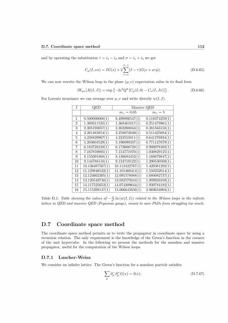
D.7. Coordinate space method 112
and by operating the substitution τ = i1 − i2 and σ = i1 + i2 we get
Cµ(I, xn) = IG(x) + 2
I−1∑
τ=1
(I − τ)G(x+ aτµ). (D.6.65)
We can now rewrite the Wilson loop in the plane (µ, ν) expectation value in its final form
〈Wµν [A](I, J)〉 = exp−2e2Q2 [Cµ(I, 0)− Cν(I, Jν)]
. (D.6.66)
For Lorentz invariance we can average over µ, ν and write directly w(I, I).
I QED Massive QEDmγ = 0.05 mγ = 5
1 0.500000000(1) 0.499806547(1) 0.118374259(1)2 1.369311535(1) 1.368461017(1) 0.251479961(1)3 2.305193057(1) 2.303260044(1) 0.381563158(1)4 3.261483854(1) 3.258072049(1) 0.511425684(1)5 4.228829967(1) 4.223555011(1) 0.641276934(1)6 5.203604529(1) 5.196090337(1) 0.771127679(1)7 6.183728249(1) 6.173606728(1) 0.900978402(1)8 7.167859805(1) 7.154771070(1) 1.030829125(1)9 8.155091868(1) 8.138684452(1) 1.160679847(1)10 9.144788116(1) 9.124719122(1) 1.290530569(1)11 10.136487567(1) 10.112422767(1) 1.420381292(1)12 11.129846532(1) 11.101460414(1) 1.550232014(1)13 12.124602305(1) 12.091578088(1) 1.680082737(1)14 13.120549740(1) 13.082579344(1) 1.809933459(1)15 14.117525653(1) 14.074309644(1) 1.939784182(1)16 15.115398147(1) 15.066645656(1) 2.069634904(1)
Table D.1: Table showing the values of − 2q2 ln (w(I, I)) related to the Wilson loops in the infinite
lattice in QED and massive QED (Feynman gauge), meant to save PhDs from struggling too much.
D.7 Coordinate space methodThe coordinate space method permits us to write the propagator in coordinate space by using arecursion relation. The only requirement is the knowledge of the Green’s function in the cornersof the unit hypercube. In the following we present the methods for the massless and massivepropagator, useful for the computation of the Wilson loops.
D.7.1 Luscher-WeiszWe consider an infinite lattice. The Green’s function for a massless particle satisfies
∑
µ
∂−µ ∂+µG(x) = δ(x). (D.7.67)
D.7. Coordinate space method 113
We know that in the continuum limit (x→∞) G(x) converges to (4π2x2)−1, the Green’s functionof the continuum laplacian in R4. We would like to express the propagator through its values closeto the origin. The key observation made by Vohwinkel is that
(∂−µ + ∂+
µ
)G(x) = xµH(x) , (D.7.68)
with the following identifications
H(x) =
∫ πa
−πa
d4p
(2π)4eip·x ln(p2),
G(x) =
∫ πa
−πa
d4p
(2π)4
eip·x
p2. (D.7.69)
Proof of the formulaTo prove the relation we calculate the l.h.s. of Eq. D.7.68
∂+µG(x) = G(x+ aµ)−G(x) =
∫ πa
−πa
d4p
(2π)4
1
p2∂+µ eip·x =
∫ πa
−πa
d4p
(2π)4
1
p2
eip·x
a
(eiapµ − 1
),
∂−µ G(x) = G(x)−G(x− aµ) =
∫ πa
−πa
d4p
(2π)4
1
p2∂+µ eip·x =
∫ πa
−πa
d4p
(2π)4
1
p2
eip·x
a
(1− e−iapµ
),
(∂−µ + ∂+
µ
)G(x) =
∫ πa
−πa
d4p
(2π)4
eip·x
p2i
[2
asin (apµ)
]. (D.7.70)
We now integrate by parts the r.h.s. of Eq. D.7.68
xµH(x) =
∫ πa
−πa
d4p
(2π)4xµeip·x ln(p2) =
∫ πa
−πa
d4p
(2π)4
(−i d
dpµeip·x
)ln(p2)
= −i∫ π
a
−πa
d4p
(2π)4
ddpµ
[eip·x ln(p2)
]+ i
∫ πa
−πa
d4p
(2π)4eip·x
(d
dpµln(p2)
). (D.7.71)
The first term vanishes since
∫ πa
−πa
d4p
(2π)4
ddpµ
[eip·x ln(p2)
]=
∫ π
a
−πa
∏
ν 6=µ
dpν(2π3)
eipνxν
∫ π
a
−πa
dpµ2π
ddpµ
[eipµxµ ln(p2)
]
=
∫ π
a
−πa
∏
ν 6=µ
dpν(2π4)
eipνxν
[eipµxµ ln(p2)
]π/a−π/a = 0 . (D.7.72)
The result is
xµH(x) =
∫ πa
−πa
d4p
(2π)4
eip·x
p22ipµ cos
(apµ2
)=
∫ πa
−πa
d4p
(2π)4
eip·x
p2i
[2
asin (apµ)
], (D.7.73)
which prove the equation Eq. D.7.68.
D.7. Coordinate space method 114
Recursion formulaWe can eliminate H(x) in Eq. D.7.68 by using Eq. D.7.67. We start by notice that
3∑
µ=0
∂−µ ∂+µ =
1
2
3∑
µ=0
(∂+µ − ∂−µ
), (D.7.74)
and by taking Eq. D.7.67 we have
3∑
µ=0
∂−µ ∂+µG(x) = 0 =
1
2
3∑
µ=0
(∂+µ − ∂−µ
)G(x) =⇒
3∑
µ=0
∂+µG(x) =
3∑
µ=0
∂−µ G(x). (D.7.75)
Now we sum over µ of Eq. D.7.68, and define ρ =∑µ xµ,
∑µ
(∂−µ + ∂+
µ
)G(x) = 2
∑3µ=0 ∂
−µ G(x)
∑µ xµH(x) = ρH(x)
H(x) =
2
ρ
3∑
µ=0
∂−µ G(x) . (D.7.76)
In this way we have eliminated the function H(x) and we can rewrite Eq. D.7.68 as
(∂−µ + ∂+
µ
)G(x) =
2xµρ
3∑
µ=0
∂−µ G(x). (D.7.77)
We can now relate the value of the propagator at a point x+ aµ to the neighbor points
G(x+ aµ) = G(x− aµ) +2xµρ
3∑
µ=0
[G(x)−G(x− aν)] , (D.7.78)
for ρ 6= 0. The propagator is independent of the sign and the order of the coordinates (x0, x1, x2, x3),from its asymptotic expansion (Luscher and Weisz, 1995). We can restrict the attention to thepoints x = an with n3 ≥ n2 ≥ n1 ≥ n0 and the recursion relation allows us to express G(x) as acombination of the propagators at the corners of the unit hypercube.Then the 5 initial values are further restricted when we take into account the following relations:
G(0, 0, 0, 0)−G(0, 0, 0, 1) =1
8a2,
G(0, 0, 0, 0)− 3G(0, 0, 1, 1)− 2G(0, 1, 1, 1) =1
a2π2,
G(0, 0, 0, 0)− 6G(0, 0, 1, 1)− 8G(0, 1, 1, 1)− 3G(1, 1, 1, 1) = 0. (D.7.79)
In the end the only initial values we have to put are
a2G(0, 0, 0, 0) = 0.154933390231060214084837208107 . . .
a2G(0, 0, 1, 1) = 0.012714703770934215428228758391 . . . (D.7.80)
The best values of the constants related to G(0, 0, 0, 0) and G(0, 0, 1, 1) are given in (Capitani,2003).

D.7. Coordinate space method 115
D.7.2 Borasoy-KrebsThe generalization in the case of a massive propagator is done in Ref. (Borasoy and Krebs, 2005).The Green’s function satisfies the equation
(m2γ +
∑
µ
∂−µ ∂+µ
)G(x) = δ(x), (D.7.81)
and it still satisfies the Eq. D.7.68 with modified functions
H(x) =
∫ πa
−πa
d4p
(2π)4eip·x ln(p2 +m2
γ),
G(x) =
∫ πa
−πa
d4p
(2π)4
eip·x
p2 +m2γ
. (D.7.82)
By following the same lines of arguments in the case of the Luscher-Weisz method we get that therecursion formula in the case of a massive propagator is given by
G(x+ aµ) = G(x− aµ) +2xµρ
3∑
µ=0
[(1 +
m2γ
8
)G(x)−G(x− aν)
]. (D.7.83)
Now the 5 initial seeds are given by the modified Bessel functions In,
G(x0, x1, x2, x3) =1
2
∫ ∞
0
dλ exp[−m2
γλ/2− 4λ]Ix0(λ)Ix1(λ)Ix2(λ)Ix3(λ). (D.7.84)
The seeds used in this work are generated using MATHEMATICA. Special thanks are given toLangæble, who helped me in writing a code free of raund-off errors.

Appendix E
Electromagnetic critical mass shift inlattice perturbation theory
In this appendix we calculate from first principle the critical mass shift induced by electromagneticeffects, to this purpose we use lattice perturbation theory. The different diagrams are calculated,this was done in order to be able to introduce a mass term for the photon, even though it is notpresented here the modification is straightforward.
E.1 Feynman rules of the Wilson theoryThe Dirac-Wilson action on the lattice is, with r = 1,
SL =∑
n∈Λ
ψf (n)
γµ∇+µ +∇−µ
2− ∇
+µ∇−µ2
+mf0
ψf (n)
=∑
n∈Λ
ψf (n)
(mf
0 + 4)ψf (n) +
1
2
∑
µ
[ψf (n)(γµ − 1)Uµ(n)ψf (n+ µ)
− ψf (n)(γµ + 1)U†µ(n− µ)ψf (n− µ)]. (E.1)
E.1.1 Photon propagator
γµ ν ≡ 1
k2
[δµν + (1− α)
kµkν
k2
]α=1=
δµν
k2.
(E.2)
E.1.2 Fermion propagator
p≡ m+ r
2 p2 − i/p
(m+ r
2 p2)2
+ p2,
(E.3)
where we defined pµ = sin(pµ).
116
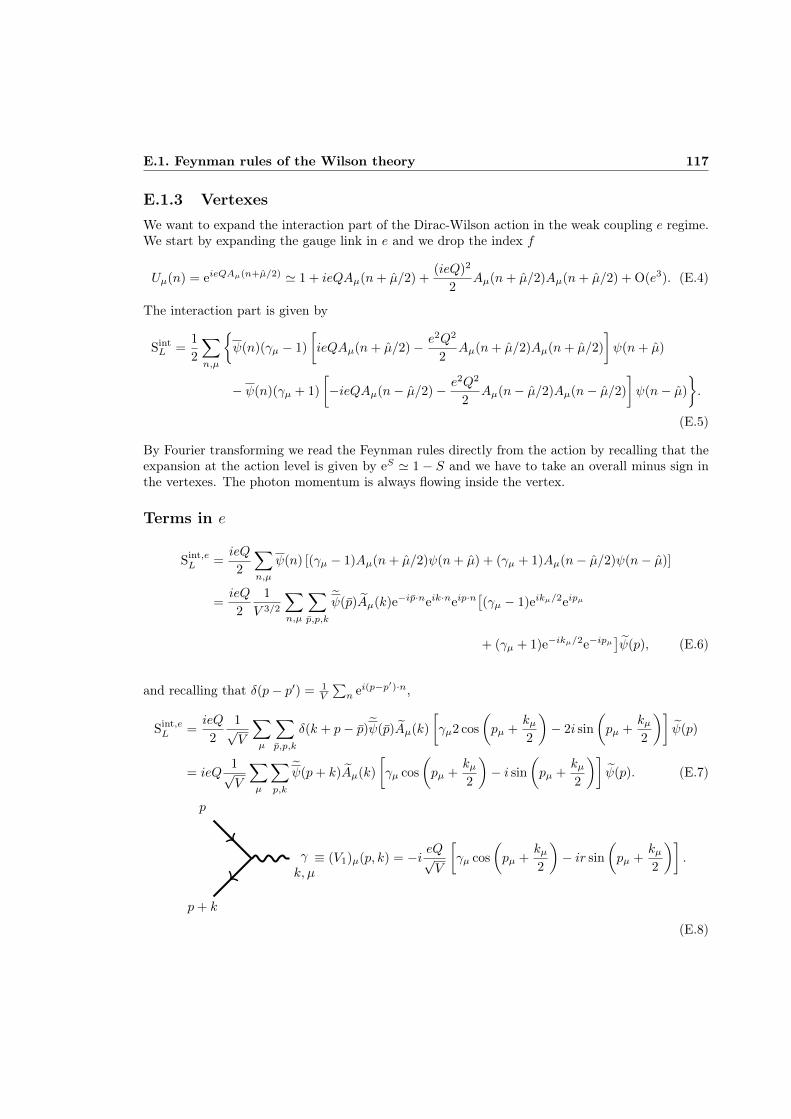
E.1. Feynman rules of the Wilson theory 117
E.1.3 VertexesWe want to expand the interaction part of the Dirac-Wilson action in the weak coupling e regime.We start by expanding the gauge link in e and we drop the index f
Uµ(n) = eieQAµ(n+µ/2) ' 1 + ieQAµ(n+ µ/2) +(ieQ)2
2Aµ(n+ µ/2)Aµ(n+ µ/2) + O(e3). (E.4)
The interaction part is given by
SintL =
1
2
∑
n,µ
ψ(n)(γµ − 1)
[ieQAµ(n+ µ/2)− e2Q2
2Aµ(n+ µ/2)Aµ(n+ µ/2)
]ψ(n+ µ)
− ψ(n)(γµ + 1)
[−ieQAµ(n− µ/2)− e2Q2
2Aµ(n− µ/2)Aµ(n− µ/2)
]ψ(n− µ)
.
(E.5)
By Fourier transforming we read the Feynman rules directly from the action by recalling that theexpansion at the action level is given by eS ' 1− S and we have to take an overall minus sign inthe vertexes. The photon momentum is always flowing inside the vertex.
Terms in e
Sint,eL =
ieQ
2
∑
n,µ
ψ(n) [(γµ − 1)Aµ(n+ µ/2)ψ(n+ µ) + (γµ + 1)Aµ(n− µ/2)ψ(n− µ)]
=ieQ
2
1
V 3/2
∑
n,µ
∑
p,p,k
ψ(p)Aµ(k)e−ip·neik·neip·n[(γµ − 1)eikµ/2eipµ
+ (γµ + 1)e−ikµ/2e−ipµ]ψ(p), (E.6)
and recalling that δ(p− p′) = 1V
∑n e
i(p−p′)·n,
Sint,eL =
ieQ
2
1√V
∑
µ
∑
p,p,k
δ(k + p− p)ψ(p)Aµ(k)
[γµ2 cos
(pµ +
kµ2
)− 2i sin
(pµ +
kµ2
)]ψ(p)
= ieQ1√V
∑
µ
∑
p,k
ψ(p+ k)Aµ(k)
[γµ cos
(pµ +
kµ2
)− i sin
(pµ +
kµ2
)]ψ(p). (E.7)
γ
k, µ
p
p+ k
≡ (V1)µ(p, k) = −i eQ√V
[γµ cos
(pµ +
kµ2
)− ir sin
(pµ +
kµ2
)].
(E.8)

E.1. Feynman rules of the Wilson theory 118
Terms in e2
This is going to be an irrelevant vertex, meaning that in the continuum there is no counterpart
Sint,e2L = −e
2Q2
4
∑
n,µ
ψ(n)[(γµ − 1)Aµ(n+ µ/2)Aµ(n+ µ/2)ψ(n+ µ)
− (γµ + 1)Aµ(n− µ/2)Aµ(n− µ/2)ψ(n− µ)]
= −e2Q2
4
1
V 2
∑
n,µ
∑
p,p,k1,k2
ψ(p)Aµ(k1)Aµ(k2)e−ip·neik1·neik2·neip·n[(γµ − 1)ei(k1,µ+k2,µ)/2eipµ
− (γµ + 1)e−i(k1,µ+k2,µ)/2e−ipµ]ψ(p)
= −e2Q2
4
1
V
∑
µ
∑
p,p,k1,k2
δ (p+ k1 + k2 − p) ψ(p)Aµ(k1)Aµ(k2)
[γµ2i sin
(pµ +
k1,µ + k2,µ
2
)
− 2 cos
(pµ +
k1,µ + k2,µ
2
)]ψ(p)
= −e2Q2
2
1
V
∑
µ
∑
p,k1,k2
ψ(p+ k1 + k2)Aµ(k1)Aµ(k2)
[γµi sin
(pµ +
k1,µ + k2,µ
2
)
− cos
(pµ +
k1,µ + k2,µ
2
)]ψ(p). (E.9)
γ
k1, µ
γk2, ν
p
p+ k1 + k2
≡ (V2)µ,ν(p, k1, k2) =e2Q2
2Vδµν
[γµi sin
(pµ +
k1,µ + k2,µ
2
)
−r cos
(pµ +
k1,µ + k2,µ
2
)].
(E.10)
E.1.4 Clover termThe clover term in the action is given by (dropping the flavor index f)
Sclover = − i4rcsw
∑
n∈Λ
∑
µ,ν
ψ(n)σµνψ(n)Fµν , (E.11)
where σµν = 12 [γµ, γν ] and Fµν = 1
8i [Qµν(n)−Qνµ(n)], with the definition
Qµν(n) =Uµ(n)Uν(n+ µ)U†µ(n+ ν)U†ν (n) + Uν(n)U†µ(n− µ+ ν)U†ν (n− µ)Uµ(n− µ)
+ U†µ(n− µ)U†ν (n− µ− ν)Uµ(n− µ− ν)Uν(n− ν)
+ U†ν (n− ν)Uµ(n− ν)Uν(n+ µ− ν)U†µ(n). (E.12)
E.1. Feynman rules of the Wilson theory 119
The multiplication of two link is simply the sum of the exponent since we are dealing with anabelian group, i.e.
Uµ(n)Uν(n) = eieQ[Aµ(n+µ/2))+Aν(n+ν/2))]. (E.13)
By expanding Eq. E.12 linearly in e, we obtain for Qµν
Qeµν = ieQ
[((((
((Aµ(n+ µ/2) +Aν(n+ µ+ ν/2)−Aµ(n+ ν + µ/2)−((((((Aν(n+ ν/2)
+((((((Aν(n+ ν/2) −Aµ(n− µ/2 + ν)−Aν(n− µ+ ν/2) +((((
((Aµ(n− µ/2)
−((((((
Aµ(n− µ/2) −Aν(n− µ− ν/2) +Aµ(n− µ/2− ν) +((((((Aν(n− ν/2)
−((((((Aν(n− ν/2) +Aµ(n+ µ/2− ν) +Aν(n+ µ− ν/2)−((((((
Aµ(n+ µ/2)
]. (E.14)
By direct inspection in QED we have that Qeµν = −Qeνµ, i.e. the Q(e) is antisymmetric and it iscontracted, in the action, with σµν (which is also antisymmetric). The result is that even powers ine vanish because the second order in e is given by the square of the first order, that is symmetric,Qe
2
µν =(Qeµν
)2= Qe
2
νµ, contracted with an antisymmetric tensor. The first order in e of F is thengiven by
F (e)µν =
1
8i2Q(e)
µν =1
4i(ieQ)
[Aν(n+ µ+ ν/2)−Aµ(n+ ν + µ/2)−Aµ(n− µ/2 + ν)−Aν(n− µ+ ν/2)
−Aν(n− µ− ν/2) +Aµ(n− µ/2− ν) +Aµ(n+ µ/2− ν) +Aν(n+ µ− ν/2)
]. (E.15)
Since we want to calculate the extra vertexes coming from the clover term we take clover actionat the first order in e and we perform the Fourier transform
Seclover = − i4
rcswV 3/2
eQ
4
∑
n,µν
∑
p,p,k
ψ(p)σµνψ(p)ei(p+k−p)·n
×[eikµeikν/2Aν(k)− eikµ/2eikν Aµ(k)− e−ikµ/2eikν Aµ(k)− eikν/2e−ikµAν(k)
− e−ikν/2e−ikµAν(k)− e−ikµ/2e−ikν Aµ(k) + eikµ/2e−ikν Aµ(k) + e−ikν/2eikµAν(k)
]
= − ir16
eQ csw√V
∑
µν
∑
p,k
ψ(p+ k)σµνψ(p)
Aν(k)2i sin kµ
[eikν/2 + e−ikν/2
]
+ Aµ(k)2 cos
(kµ2
)[e−ikν − eikν
]
= − i2r
16
eQ csw√V
4∑
µν
∑
p,k
ψ(p+ k)σµνψ(p)
Aν(k) sin kµ cos
(kν2
)− Aµ(k) sin kν cos
(kµ2
).
(E.16)
By renaming the first term µ↔ ν and using that σµν is antisymmetric we get
Seclover = −r2
eQ csw√V
∑
µν
∑
p,k
ψ(p+ k)σµνψ(p)Aµ(k) sin kν cos
(kµ2
), (E.17)

E.2. Electromagnetic fermion self-energy 120
from which we read the associated vertex
γ
k, µ
p
p+ k
≡ (Vc)µ(p, k) =r eQ csw
2√V
∑
ν
σµν sin kν cos
(kµ2
).
(E.18)
E.2 Electromagnetic fermion self-energyWe want to compute the 1-loop contribution to the quark self-energy, the Feynman diagramscontributing are the following ones.
Tadpole in Feynman gauge
IFeynT =
k
p p
∣∣∣∣p=0,m=0
=∑
k
∑
µ,ν
(V2)µν(0,−k, k)Gµν(k)
=∑
k
∑
µ,ν
δµν(−r)e2Q2
2V
δµν
k2= −e
2Q2
V
r
2
∑
k
4
k2. (E.19)
Tadpole in Coulomb gaugeIn order to calculate the tadpole diagram in Coulomb gauge it is sufficient to use the followinggauge transformation
ACµ (p) =
∑
ν
[δµν −
pµ ·(0, p)ν
|p|2
]Aν(p), (E.20)
where A is the field generated in Feynman gauge and AC the field in Coulomb gauge.For the tadpole it is sufficient to calculate the propagator in Coulomb gauge
〈ACµ A
Cν 〉 =
∑
ρ,σ
[δµρ −
pµ ·(0, p)ρ
|p|2
][δνσ −
pν ·(0, p)σ
|p|2
]〈Aρ(p)Aσ(p)〉
=∑
ρ,σ
[δµρδνσ −
δνσpµ ·(0, p)ρ
+ δµρpν ·(0, p)σ
|p|2 +pµ ·
(0, p)ρpν ·
(0, p)σ
(|p|2)2
]〈Aρ(p)Aσ(p)〉
= 〈Aµ(p)Aν(p)〉 −∑
ρ
pµ ·(0, p)ρ
|p|2 〈Aρ(p)Aν(p)〉
−∑
σ
pν ·(0, p)σ
|p|2 〈Aµ(p)Aσ(p)〉+∑
ρ,σ
pµ ·(0, p)ρpν ·
(0, p)σ
(|p|2)2〈Aρ(p)Aν(p)〉

E.2. Electromagnetic fermion self-energy 121
=δµνp2−∑
ρ
pµ ·(0, p)ρ
|p|2δρνp2−∑
σ
pν ·(0, p)σ
|p|2δµσp2
+∑
ρ,σ
pµ ·(0, p)ρpν ·
(0, p)σ
(|p|2)2
δρσp2
=δµνp2−pµ ·
(0, p)ν
+ pν ·(0, p)µ
p2 |p|2 +∑
ρ
pµ ·(0, p)ρpν ·
(0, p)ρ
p2 (|p|2)2. (E.21)
Now we can insert the propagator in the tadpole and calculate the value of the integral in Coulombgauge
ICoulT = −e
2Q2
V
r
2
∑
k
∑
µ
1
k2− 2
kµ ·(
0, k)µ
k2 |k|2+k2µ
∑j k
2
j
k2 (|k|2)2
= −e
2Q2
V
r
2
∑
k
[4
k2− 2
∑j k
2j
k2 |k|2+
k2
k2 |k|2
]
= −e2Q2
V
r
2
∑
k
[4
k2− 2
k2+
1
|k|2
]= −e
2Q2
V
r
2
∑
k
[2
k2+
1
|k|2
]. (E.22)
The tadpole result in Coulomb gauge is the same quoted in Ref. (Duncan et al., 1996).
Sunset in Feynman gauge
IFeynS =
k
p− kp p
µ ν
∣∣∣∣p=0,m=0
=∑
k
∑
µ,ν
(V1)ν(−k, 0)S(−k)(V1)µ(0,−k)Gµν(k)
= −e2Q2
V
∑
k
∑
µ,ν,σ
δµν
k2
[γν cos
(kν2
)+ ir sin
(kν2
)] r2 k
2σ + iγσkσ
r2
4
(k2)2
+ k2
×[γµ cos
(kµ2
)+ ir sin
(kµ2
)]. (E.23)
We retain only the even functions of k since the integration is done in a symmetric interval, thisgives us
IFeynS =− e2Q2
V
∑
k
∑
µ,σ
1
k2
1
r2
4
(k2)2
+ k2
[γ2µ
r
2k2σ cos2
(kµ2
)+ γµγσ(i)2rkσ sin
(kµ2
)cos
(kµ2
)
+ (ir)2 r
2sin2
(kµ2
)k2σ + γσγµ(i)2rkσ sin
(kµ2
)cos
(kµ2
)]
=− e2Q2
V
∑
k
∑
µ,σ
1
k2
1
r2
4
(k2)2
+ k2
[r
2k2σ
(1− sin2
(kµ2
))− rkσ
1
2sin (kµ) γµ, γσ︸ ︷︷ ︸
2δµσ
− r3
2sin2
(kµ2
)k2σ
]
=− e2Q2
V
∑
k
∑
µ,σ
1
k2
1
r2
4
(k2)2
+ k2
[r
2k2σ
(1− k2
µ
4
)− rkσkµδµσ −
r3
2
k2µ
4k2σ
]

E.2. Electromagnetic fermion self-energy 122
=− e2Q2
V
∑
k
1
k2
r
r2
4
(k2)2
+ k2
[k2
2
(1− k2
4
)− k2 − r2
2
(k2)2
4
]
=− e2Q2
Vr∑
k
1
k2
1
r2
4
(k2)2
+ k2
[2k2 − (k2)2
8− k2 − r2
8(k2)2 − k2
2+k2
2
]
=− e2Q2
V
r
2
∑
k
1
k2
k2(
4− k2/4)− k2
r2
4
(k2)2
+ k2
− 1
. (E.24)
Clover sunset in Feynman gauge
IFeynCS =
k
p− kp p
µ ν
∣∣∣∣p=0,m=0
=∑
k
∑
µ,ν
(Vc)ν(−k, 0)S(−k)(Vc)µ(0,−k)Gµν(k)
=r2c2swe
2Q2
4V
∑
k
∑
µ,ν,ρ,σ,γ
δµν
k2
[−σνρ sin kρ cos
(kν2
)] r2 k
2γ + iγγ kγ
r2
4
(k2)2
+ k2
σµσ sin kσ cos
(kµ2
).
(E.25)
As usual we take only the even powers in k and we get
IFeynCS = −r
3c2swe2Q2
8V
∑
k,µ,ρ,σ
k2
k2
σµρσµσkσkρ
(1− k2
µ/4)
r2
4
(k2)2
+ k2
. (E.26)
We need to find what is the product of the two antisymmetric tensors
4σµρσµσ = [γµ, γρ][γµ, γσ] = (γµγρ − γργµ) (γµγσ − γσγµ) = 4δρσδµσ − 2γµγργσγµ − 2γrhoγσ.(E.27)
The product σµρσµσ is contracted with kσkρ that is symmetric with respect to σ and ρ, this meanswe can retain only the symmetric part of the product with respect to σ and ρ, i.e.
4σµρσµσkσkρ = 4δρσδµσkσkρ − 2γµ1
2γρ, γσγµkσkρ − 2
1
2γρ, γσkσkρ
= 4δρσδµσkσkρ − 2δρσkσkρ − 2δρσkσkρ = 4kσkρ (δρσδµσ − δρσ) . (E.28)
The substituting back in the original integral we get
IFeynCS = −r
3c2swe2Q2
8V
∑
k,µ,ρ,σ
1− k2µ/4
r2
4
(k2)2
+ k2
kσkρ (δρσδµσ − δρσ) . (E.29)
The first term in the parentheses gives∑
µ,ρ,σ
(1− k2
µ/4)kσkρδρσδµσ =
∑
µ,σ
(1− k2
µ/4)k2σδµσ =
∑
µ
(1− k2
µ/4)k2µ
= k2 − 1
4
∑
µ
k2µk
2µ = k2 − 1
4k4 +
1
16k6, (E.30)
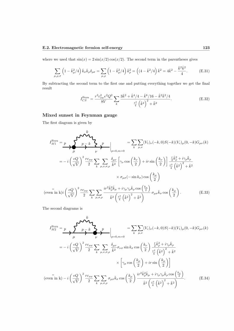
E.2. Electromagnetic fermion self-energy 123
where we used that sin(x) = 2 sin(x/2) cos(x/2). The second term in the parentheses gives
∑
µ,ρ,σ
(1− k2
µ/4)kσkρδρσ =
∑
µ,ρ
(1− k2
µ/4)k2ρ =
((4− k2/4
)k2 = 4k2 − k2k2
4. (E.31)
By subtracting the second term to the first one and putting everything together we get the finalresult
IFeynCS =
r3c2swe2Q2
8V
∑
k
3k2 + k4/4− k6/16− k2k2/4
r2
4
(k2)2
+ k2
. (E.32)
Mixed sunset in Feynman gaugeThe first diagram is given by
IFeynM1 =
k
p− kp p
µ ν
∣∣∣∣p=0,m=0
=∑
k
∑
µ,ν
(V1)ν(−k, 0)S(−k)(Vc)µ(0,−k)Gµν(k)
=− i(eQ√V
)2rcsw
2
∑
k
∑
µ,ν,σ,ρ
δµν
k2
[γν cos
(kν2
)+ ir sin
(kν2
)] r2 k
2ρ + iγρkρ
r2
4
(k2)2
+ k2
× σµσ(− sin kσ) cos
(kµ2
)
=
(even in k)i
(eQ√V
)2rcsw
2
∑
k
∑
µ,σ,ρ
ir2k2ρkµ + iγµγρkρ cos
(kµ2
)
k2
(r2
4
(k2)2
+ k2
) σµσkσ cos
(kµ2
). (E.33)
The second diagrams is
IFeynM2 =
k
p− kp p
µ ν
∣∣∣∣p=0,m=0
=∑
k
∑
µ,ν
(Vc)ν(−k, 0)S(−k)(V1)µ(0,−k)Gµν(k)
=− i(eQ√V
)2rcsw
2
∑
k
∑
µ,ν,σ,ρ
δµν
k2σνσ sin kσ cos
(kν2
) r2 k
2ρ + iγρkρ
r2
4
(k2)2
+ k2
×[γµ cos
(kµ2
)+ ir sin
(kµ2
)]
=
(even in k)− i(eQ√V
)2rcsw
2
∑
k
∑
µ,σ,ρ
σµσkσ cos
(kµ2
) ir2k2ρkµ + iγργµkρ cos
(kµ2
)
k2
(r2
4
(k2)2
+ k2
) . (E.34)

E.2. Electromagnetic fermion self-energy 124
By putting the two diagrams together the terms with σµσ cancel out because of its antisymmetricnature and we are left with
IFeynM1 + IFeyn
M2 =e2Q2
V
rcsw2
∑
k
1
k2
(r2
4
(k2)2
+ k2
)∑
µ,σ,ρ
kσkρ cos2
(kµ2
)(σµσγργµ − γµγρσµσ)
=e2Q2
V
rcsw2
∑
k,µ,σ,ρ
kσkρ
(1− k2
µ/4)
k2
(r2
4
(k2)2
+ k2
) (σµσγργµ − γµγρσµσ) . (E.35)
The term with the antisymmetric tensor gives
(σµσγργµ − γµγρσµσ) =1
2δρσ −
1
2δσµδρµ, (E.36)
and collecting everything we get
IFeynM1 + IFeyn
M2 =e2Q2
V
rcsw4
∑
k,µ,σ,ρ
kσkρ
(1− k2
µ/4)
k2
(r2
4
(k2)2
+ k2
) (δρσ − δσµδρµ)
=e2Q2
V
rcsw4
∑
k
1
k2
(r2
4
(k2)2
+ k2
)(∑
µ,ρ
k2ρ
(1− k2
µ/4)−∑
µ
k2µ
(1− k2
µ/4))
=e2Q2
V
rcsw4
∑
k
3k2 + k4/4− k6/16− k2k2/4
k2
(r2
4
(k2)2
+ k2
) . (E.37)
Self-energy resummation
We symbolically write the self-energy at 1-loop as
Σ1(p;m, e2) = = + ,
where for simplicity we assume the sunset diagram to be the sum of the ones with different vertexesinsertion, without loss of generality.

E.2. Electromagnetic fermion self-energy 125
By summing insertions of self-energy at 1-loop we get that the dressed propagator is given by
= + +
+ + + . . .
= + + + . . .
=
(1 + + + . . .
)
=
(∞∑
k=0
)=
1−
=1
m + r2p2 + i/p− Σ1(p;m, e2)
,
where we noticed that the series of insertions of self-energy give rise to the geometric series. TheΣ1(p;m, e2) is a function of the bare parameters. Now we add a mass counterterm to the Lagrangianδmψψ that gives the following additional vertex
× ≡ δm . (E.38)
We interpret the renormalized mass as mR = m + δm and replace in the self-energy calculationsm with mR: Σ1(p;m, e2)→ Σ1(p;mR, e
2). The inverse propagator gets modified as
mR +r
2p2 + i/p−
(Σ1(p;mR, e
2) + δm). (E.39)
We require that the propagator has a pole when the renormalized mass and momentum vanishes,i.e. mR = 0 and p = 0. By imposing the condition we get the value of δm
mR +r
2p2 + i/p−
(Σ1(p;mR, e
2) + δm) ∣∣∣∣mR=0,p=0
= −Σ1(p = 0;mR = 0, e2)− δm = 0
⇒ δm = −Σ1(p = 0;mR = 0, e2) = −(
p p + p p
)
mR=0,p=0
.
(E.40)
The critical mass mc is the bare mass for which the renormalized mass is vanishing, i.e. mc = −δm,and in terms of that we have the following relation
mR = m−mc = m− Σ1(p = 0;mR = 0, e2) = m− (IT + IS + ICS + IM1 + IM2) . (E.41)
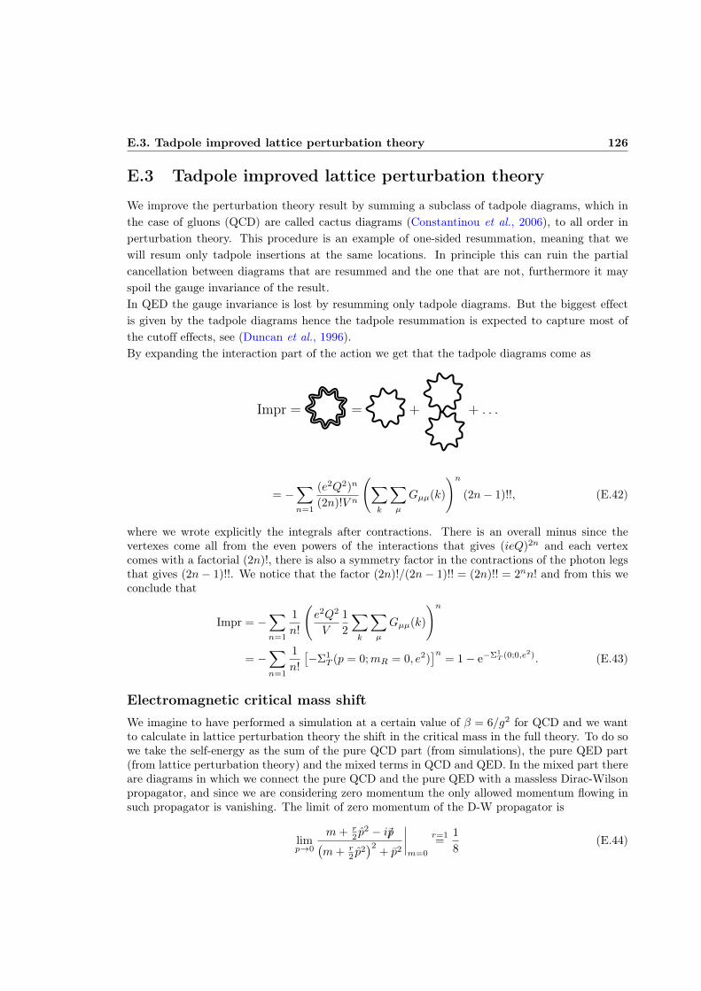
E.3. Tadpole improved lattice perturbation theory 126
E.3 Tadpole improved lattice perturbation theory
We improve the perturbation theory result by summing a subclass of tadpole diagrams, which inthe case of gluons (QCD) are called cactus diagrams (Constantinou et al., 2006), to all order inperturbation theory. This procedure is an example of one-sided resummation, meaning that wewill resum only tadpole insertions at the same locations. In principle this can ruin the partialcancellation between diagrams that are resummed and the one that are not, furthermore it mayspoil the gauge invariance of the result.In QED the gauge invariance is lost by resumming only tadpole diagrams. But the biggest effectis given by the tadpole diagrams hence the tadpole resummation is expected to capture most ofthe cutoff effects, see (Duncan et al., 1996).By expanding the interaction part of the action we get that the tadpole diagrams come as
Impr = = + + . . .
= −∑
n=1
(e2Q2)n
(2n)!V n
(∑
k
∑
µ
Gµµ(k)
)n(2n− 1)!!, (E.42)
where we wrote explicitly the integrals after contractions. There is an overall minus since thevertexes come all from the even powers of the interactions that gives (ieQ)2n and each vertexcomes with a factorial (2n)!, there is also a symmetry factor in the contractions of the photon legsthat gives (2n− 1)!!. We notice that the factor (2n)!/(2n− 1)!! = (2n)!! = 2nn! and from this weconclude that
Impr = −∑
n=1
1
n!
(e2Q2
V
1
2
∑
k
∑
µ
Gµµ(k)
)n
= −∑
n=1
1
n!
[−Σ1
T (p = 0;mR = 0, e2)]n
= 1− e−Σ1T (0;0,e2). (E.43)
Electromagnetic critical mass shiftWe imagine to have performed a simulation at a certain value of β = 6/g2 for QCD and we wantto calculate in lattice perturbation theory the shift in the critical mass in the full theory. To do sowe take the self-energy as the sum of the pure QCD part (from simulations), the pure QED part(from lattice perturbation theory) and the mixed terms in QCD and QED. In the mixed part thereare diagrams in which we connect the pure QCD and the pure QED with a massless Dirac-Wilsonpropagator, and since we are considering zero momentum the only allowed momentum flowing insuch propagator is vanishing. The limit of zero momentum of the D-W propagator is
limp→0
m+ r2 p
2 − i/p(m+ r
2 p2)2
+ p2
∣∣∣∣m=0
r=1=
1
8(E.44)

E.3. Tadpole improved lattice perturbation theory 127
In this way we are including all the possible non-1PI diagrams built out of Q(C+E)D. Diagram-matically the self-energy is
Σ(p = 0;m = 0) = ' + + + +
+ + .
The formula reads
Σ(p = 0;m = 0) ' Σe(0; 0) + Σg(0; 0) + 2Σe(0; 0) limk→0
S(k)Σg(0; 0)
= Σe(0; 0) + Σg(0; 0) +Σe(0; 0)Σg(0; 0)
4, (E.45)
where we have a factor two in the last addendum because of the symmetry of the diagrams.Recalling that the critical mass (or the self-energy Σ) is related to the critical κ (hopping parameter)
κc =1
8r + 2Σ(0; 0), (E.46)
we get that
∆mQ(C+E)Dc ' Σ(0; 0)− Σg(0; 0) =
1
2κc− 1
2κe=0c
= Σe(0; 0) +1
4Σe(0; 0)Σg(0; 0)
= Σe(0; 0) +1
4Σe(0; 0)
(1
2κe=0c
− 4
)=
Σe(0; 0)
8κe=0c
. (E.47)
We found the electromagnetic shift to the critical mass in the approximation where we sum onlythe self-energies from QCD and QED connected by a fermion line.We can approximate the EM self-energy with 1-loop result and write
∆mQ(C+E)Dc ' Σ1
e(0; 0)
8κe=0c
. (E.48)
We can also take as approximate EM self-energy the tadpole resummed one in Eq. E.43 we getthat the shift is given by
∆mQ(C+E)Dc ' ΣT
e (0; 0)
8κe=0c
=1
8κe=0c
(1− e−Σ1
T (0;0,e2))
=1
8κe=0c
(1− eδmem
). (E.49)
Appendix F
Explicit form of the HVP
Here we perform the Wick contractions for Eq. 5.3.29, and we set r = 1. As an example we workout only the following contribution, one out of four,
1
4
∑
f,f ′
[ψf (n+ µ)(1 + γµ)U†µ(n)ψf (n)
] [ψf ′(ν)(1 + γν)U†ν (0)ψf ′(0)
]. (F.1)
We write all the indexes out, f, f ′ are the flavor ones, α, β, γ, δ the Dirac ones and b, c, d thecolor ones, and we calculate the fermionic part of the expectation value (〈. . . 〉F =
∏Nff 〈. . . 〉f) that
factorizes with respect to flavor
I =1
4
∑
f,f ′
⟨ψa,α
f (n+ µ)(1 + γµ)αβ(U†µ(n)
)abψb,βf (n)ψ
c,γ
f ′ (ν)(1 + γν)γδ(U†ν (0)
)cdψd,γf ′ (0)
⟩
F
=∑
f,f ′
1
4(1 + γµ)αβ
(U†µ(n)
)ab
(1 + γν)γδ(U†ν (0)
)cd
⟨ψa,α
f (n+ µ)ψb,βf (n)ψc,γ
f ′ (ν)ψd,γf ′ (0)
⟩
F.
(F.2)
We recall that Wick contractions give the propagator,
〈ψa,α(n)ψb,β
(m)〉 =(D−1(n,m)
)αβab, (F.3)
and can be used to obtain
I =(−1)2
4(1 + γµ)αβ
(U†µ(n)
)ab
(1 + γν)γδ(U†ν (0)
)cd
∑
f 6=f ′
⟨ψb,βf (n)ψ
a,α
f (n+ µ)
⟩
f
×⟨ψd,γf ′ (0)ψ
c,γ
f ′ (ν)
⟩
f ′+∑
f
⟨ψd,γf (0)ψ
a,α
f (n+ µ)
⟩
f
⟨ψb,βf (n)ψ
c,γ
f (ν)
⟩
f ′
=1
4(1 + γµ)αβ
(U†µ(n)
)ab
(1 + γν)γδ(U†ν (0)
)cd
∑
f 6=f ′
(D−1f (n+ µ, n)
)αβab
(D−1f ′ (ν, 0)
)δγdc
+∑
f
(D−1f (n+ µ, 0)
)αβab
(D−1f (ν, n)
)δγdc
.
(F.4)
128

Appendix F. Explicit form of the HVP 129
In the first step we used the factorization of the fermionic expectation value with respect to flavorand we divided the case in which f = f ′ and f 6= f ′, recalling that the fermionic variables areGrassmann variables and they anticommute. In the second step we performed the Wick contractionand displayed the propagator.By collecting all the indexes together we get
I =1
4
∑
f
TrD−1f (n+ µ, n)U†µ(n)(1 + γµ)
∑
f ′
TrD−1f (ν, 0)U†ν (0)(1 + γν)
︸ ︷︷ ︸disconnected piece
+1
4
∑
f
Tr
(1 + γν)U†ν (0)D−1f (n+ µ, 0)(1 + γµ)U†µ(n)D−1
f (ν, n)
︸ ︷︷ ︸connected piece
. (F.5)
By using γ5-hermiticity of the Dirac-Wilson operator (D−1 = γ5
(D†)−1
γ5) we obtain
Iconnected =1
4
∑
f
Tr
(1 + γν)U†ν (0)γ5
[(D†)−1
f(0, n+ µ)
]γ5(1 + γµ)U†µ(n)D−1
f (ν, n). (F.6)
Analogously one can calculate the other pieces of the product and eventually obtain, for theconnected part,
Πconnectedµν (n) =
1
4
∑
f
(Tr
(1 + γν)U†ν (0)γ5
[(D†)−1
f(0, n+ µ)
]γ5(1 + γµ)U†µ(n)D−1
f (ν, n)
−(1− γν)Uν(0)γ5
[(D†)−1
f(ν, n+ µ)
]γ5(1 + γµ)U†µ(n)D−1
f (0, n)
−(1 + γν)U†ν (0)γ5
[(D†)−1
f(0, n)
]γ5(1− γµ)Uµ(n)D−1
f (ν, n+ µ)
+(1− γν)Uν(0)γ5
[(D†)−1
f(ν, n)
]γ5(1− γµ)Uµ(n)D−1
f (0, n+ µ)
).
(F.7)
The contraction for Eq. 5.3.30, the contact term, are done in the same way
Πctµν(0) = −δµν
2
∑
f
⟨ψf (0)Uµ(0)(1− γµ)ψf (µ) + ψf (µ)U†µ(0)(γµ + 1)ψf (0)
⟩
F
= −δµν2
∑
f
⟨ψa,α
f (0) (Uµ(0))ab (1− γµ)αβψb,βf (µ) + ψ
a,α
f (µ)(U†µ(0)
)ab
(γµ + 1)αβψb,βf (0)
⟩
f
= (−)2 δµν2
∑
f
[(Uµ(0))ab (1− γµ)αβ
⟨ψb,βf (µ)ψ
a,α
f (0)
⟩
f
+(U†µ(0)
)ab
(γµ + 1)αβ
⟨ψb,βf (0)ψ
a,α
f (µ)
⟩
f
]

Appendix F. Explicit form of the HVP 130
=δµν2
∑
f
[(Uµ(0))ab (1− γµ)αβ
(D−1f (0, µ)
)βαba
+(U†µ(0)
)ab
(γµ + 1)αβ
(D−1f (µ, 0)
)βαba
]
=δµν2
∑
f
(Tr
(1− γµ)Uµ(0)[D−1f (0, µ)
]+ (1 + γµ)U†µ(0)
[D−1f (µ, 0)
])
=δµν2
∑
f
(Tr
(1− γµ)Uµ(0)γ5
[(D†)−1
f(µ, 0)
]γ5 + (1 + γµ)U†µ(0)
[D−1f (µ, 0)
]), (F.8)
and by recalling that γ5, γµ = 0⇒ γ5γµγ5 = −γµ and γ25 = 1, we find
Πctµν(0) =
δµν2
∑
f
(Tr
(1 + γµ)Uµ(0)[(D†)−1
f(µ, 0)
]+ (1 + γµ)U†µ(0)
[D−1f (µ, 0)
]). (F.9)
By looking at Eq. F.7 and Eq. F.9 we see that to evaluate Πµν we need to do five inversions oneach gauge field configuration, which make the calculations quite expensive in computer time.The identification with the results in the appendix of (Gockeler et al., 2004) is easily made.

Bibliography
[Amsler and others, 2008] Claude Amsler et al. Review of Particle Physics. Phys. Lett., B667:1–1340, 2008.
[Aoki and others, 2012] S. Aoki et al. 1+1+1 flavor QCD + QED simulation at the physical point.Phys. Rev., D86:034507, 2012.
[Arthur and Boyle, 2011] R. Arthur and P. A. Boyle. Step Scaling with off-shell renormalisation.Phys. Rev., D83:114511, 2011.
[Arthur et al., 2016] Rudy Arthur, Vincent Drach, Martin Hansen, Ari Hietanen, Claudio Pica,and Francesco Sannino. SU(2) gauge theory with two fundamental flavors: A minimal templatefor model building. Phys. Rev., D94(9):094507, 2016.
[Aubin et al., 2012] Christopher Aubin, Thomas Blum, Maarten Golterman, and Santiago Peris.Model-independent parametrization of the hadronic vacuum polarization and g-2 for the muonon the lattice. Phys. Rev., D86:054509, 2012.
[Basak and others, 2014] Subhasish Basak et al. Finite-volume effects and the electromagneticcontributions to kaon and pion masses. PoS, LATTICE2014:116, 2014.
[Bedaque, 2004] Paulo F. Bedaque. Aharonov-Bohm effect and nucleon nucleon phase shifts onthe lattice. Phys. Lett., B593:82–88, 2004.
[Bernecker and Meyer, 2011] David Bernecker and Harvey B. Meyer. Vector Correlators in LatticeQCD: Methods and applications. Eur. Phys. J., A47:148, 2011.
[Bloch and Nordsieck, 1937] F. Bloch and A. Nordsieck. Note on the Radiation Field of the elec-tron. Phys. Rev., 52:54–59, 1937.
[Blum and others, 2016] T. Blum et al. Lattice calculation of the leading strange quark-connectedcontribution to the muon g − 2. JHEP, 04:063, 2016. [Erratum: JHEP05,034(2017)].
[Blum et al., 2007] Thomas Blum, Takumi Doi, Masashi Hayakawa, Taku Izubuchi, and NorikazuYamada. Determination of light quark masses from the electromagnetic splitting of pseudoscalarmeson masses computed with two flavors of domain wall fermions. Phys. Rev., D76:114508, 2007.
[Blum et al., 2010] T. Blum, R. Zhou, T. Doi, M. Hayakawa, T. Izubuchi, S. Uno, and N. Yamada.Electromagnetic mass splittings of the low lying hadrons and quark masses from 2+1 flavor latticeQCD+QED. Phys. Rev., D82:094508, 2010.
[Blum et al., 2012] T. Blum, M. Hayakawa, and T. Izubuchi. Hadronic corrections to the muonanomalous magnetic moment from lattice QCD. PoS, LATTICE2012:022, 2012.
131

BIBLIOGRAPHY 132
[Blum, 2003] T. Blum. Lattice calculation of the lowest order hadronic contribution to the muonanomalous magnetic moment. Phys. Rev. Lett., 91:052001, 2003.
[Bochicchio et al., 1985] Marco Bochicchio, Luciano Maiani, Guido Martinelli, Gian Carlo Rossi,and Massimo Testa. Chiral Symmetry on the Lattice with Wilson Fermions. Nucl. Phys.,B262:331, 1985.
[Borasoy and Krebs, 2005] B. Borasoy and H. Krebs. Greens function of a free massive scalar fieldon the lattice. Phys. Rev., D72:056003, 2005.
[Borsanyi and others, 2015] Sz. Borsanyi et al. Ab initio calculation of the neutron-proton massdifference. Science, 347:1452–1455, 2015.
[Boyle et al., 2008] P. A. Boyle, A. Juttner, C. Kelly, and R. D. Kenway. Use of stochastic sourcesfor the lattice determination of light quark physics. JHEP, 08:086, 2008.
[Boyle et al., 2016] Peter Boyle, Vera Gülpers, James Harrison, Andreas Jüttner, Antonin Portelli,and Christopher Sachrajda. Electromagnetic Corrections to Meson Masses and the HVP. PoS,LATTICE2016:172, 2016.
[Brandt et al., 2013] Bastian B. Brandt, Andreas Jüttner, and Hartmut Wittig. The pion vectorform factor from lattice QCD and NNLO chiral perturbation theory. JHEP, 11:034, 2013.
[Brandt et al., 2016] Bastian B Brandt, Gunnar Bali, Gergely Endrödi, and Benjamin Glässle.QCD spectroscopy and quark mass renormalisation in external magnetic fields with Wilsonfermions. PoS, LATTICE2015:265, 2016.
[Brower et al., 1997] R. C. Brower, T. Ivanenko, A. R. Levi, and K. N. Orginos. Chronologicalinversion method for the Dirac matrix in hybrid Monte Carlo. Nucl. Phys., B484:353–374, 1997.
[Bussone and others, 2016] A. Bussone et al. Mass of the b quark and B -meson decay constantsfrom Nf=2+1+1 twisted-mass lattice QCD. Phys. Rev., D93(11):114505, 2016.
[Bussone et al., 2016a] Andrea Bussone, Michele Della Morte, Vincent Drach, Martin Hansen, AriHietanen, Jarno Rantaharju, and Claudio Pica. A simple method to optimize HMC performance.PoS, LATTICE2016:260, 2016.
[Bussone et al., 2016b] Andrea Bussone, Michele Della Morte, Martin Hansen, and Claudio Pica.Reweighting twisted boundary conditions. PoS, LATTICE2015:021, 2016.
[Bussone et al., 2017] Andrea Bussone, Michele Della Morte, Martin Hansen, and Claudio Pica.On reweighting for twisted boundary conditions. Comput. Phys. Commun., 2017.
[Capitani et al., 2015] S. Capitani, M. Della Morte, D. Djukanovic, G. von Hippel, J. Hua,B. Jäger, B. Knippschild, H. B. Meyer, T. D. Rae, and H. Wittig. Nucleon electromagneticform factors in two-flavor QCD. Phys. Rev., D92(5):054511, 2015.
[Capitani, 2003] Stefano Capitani. Lattice perturbation theory. Phys. Rept., 382:113–302, 2003.
[Carloni Calame et al., 2015] C. M. Carloni Calame, M. Passera, L. Trentadue, and G. Venanzoni.A new approach to evaluate the leading hadronic corrections to the muon g-2. Phys. Lett.,B746:325–329, 2015.
BIBLIOGRAPHY 133
[Chakraborty et al., 2016] Bipasha Chakraborty, C. T. H. Davies, J. Koponen, G. P. Lepage, M. J.Peardon, and S. M. Ryan. Estimate of the hadronic vacuum polarization disconnected con-tribution to the anomalous magnetic moment of the muon from lattice QCD. Phys. Rev.,D93(7):074509, 2016.
[Chetyrkin et al., 1996] K. G. Chetyrkin, Johann H. Kuhn, and M. Steinhauser. Three loop polar-ization function and O (alpha-s**2) corrections to the production of heavy quarks. Nucl. Phys.,B482:213–240, 1996.
[Clark and Kennedy, 2007] M. A. Clark and A. D. Kennedy. Accelerating dynamical fermion com-putations using the rational hybrid Monte Carlo (RHMC) algorithm with multiple pseudofermionfields. Phys. Rev. Lett., 98:051601, 2007.
[Clark et al., 2008] M. A. Clark, A. D. Kennedy, and P. J. Silva. Tuning HMC using Poissonbrackets. PoS, LATTICE2008:041, 2008.
[Clark et al., 2010] M. A. Clark, Balint Joo, A. D. Kennedy, and P. J. Silva. Better HMC integra-tors for dynamical simulations. PoS, LATTICE2010:323, 2010.
[Clark et al., 2011] M. A. Clark, Balint Joo, A. D. Kennedy, and P. J. Silva. Improving dynamicallattice QCD simulations through integrator tuning using Poisson brackets and a force-gradientintegrator. Phys. Rev., D84:071502, 2011.
[Constantinou et al., 2006] M. Constantinou, H. Panagopoulos, and A. Skouroupathis. Improvedperturbation theory for improved lattice actions. Phys. Rev., D74:074503, 2006.
[Creutz et al., 1979] Michael Creutz, Laurence Jacobs, and Claudio Rebbi. Monte Carlo Study ofAbelian Lattice Gauge Theories. Phys. Rev., D20:1915, 1979. [,182(1979)].
[Curci, 1986] Giuseppe Curci. Infrared Finiteness of Normalization Constants of Currents in Lat-tice Gauge Theories. Phys. Lett., B167:425–428, 1986.
[Cè et al., 2017] Marco Cè, Leonardo Giusti, and Stefan Schaefer. A local factorization of thefermion determinant in lattice QCD. Phys. Rev., D95(3):034503, 2017.
[Davoudi and Savage, 2014] Zohreh Davoudi and Martin J. Savage. Finite-Volume Electromag-netic Corrections to the Masses of Mesons, Baryons and Nuclei. Phys. Rev., D90(5):054503,2014.
[de Divitiis et al., 2004] G. M. de Divitiis, R. Petronzio, and N. Tantalo. On the discretization ofphysical momenta in lattice QCD. Phys. Lett., B595:408–413, 2004.
[de Divitiis et al., 2013] G. M. de Divitiis, R. Frezzotti, V. Lubicz, G. Martinelli, R. Petronzio,G. C. Rossi, F. Sanfilippo, S. Simula, and N. Tantalo. Leading isospin breaking effects on thelattice. Phys. Rev., D87(11):114505, 2013.
[DeGrand and Rossi, 1990] Thomas A. DeGrand and Pietro Rossi. Conditioning Techniques forDynamical Fermions. Comput. Phys. Commun., 60:211–214, 1990.
[Del Debbio et al., 2010] Luigi Del Debbio, Agostino Patella, and Claudio Pica. Higher repre-sentations on the lattice: Numerical simulations. SU(2) with adjoint fermions. Phys. Rev.,D81:094503, 2010.

BIBLIOGRAPHY 134
[Della Morte and Giusti, 2011] Michele Della Morte and Leonardo Giusti. A novel approach forcomputing glueball masses and matrix elements in Yang-Mills theories on the lattice. JHEP,05:056, 2011.
[Della Morte et al., 2012] Michele Della Morte, Benjamin Jager, Andreas Juttner, and HartmutWittig. Towards a precise lattice determination of the leading hadronic contribution to (g−2)µ.JHEP, 03:055, 2012.
[Della Morte et al., 2014] Michele Della Morte, Samantha Dooling, Jochen Heitger, Dirk Hesse,and Hubert Simma. Matching of heavy-light flavour currents between HQET at order 1/m andQCD: I. Strategy and tree-level study. JHEP, 05:060, 2014.
[Della Morte et al., 2017] M. Della Morte, A. Francis, V. Gülpers, G. Herdoíza, G. von Hippel,H. Horch, B. Jäger, H. B. Meyer, A. Nyffeler, and H. Wittig. The hadronic vacuum polarizationcontribution to the muon g − 2 from lattice QCD. 2017.
[Di Chiara et al., 2017] Stefano Di Chiara, Andrew Fowlie, Sean Fraser, Carlo Marzo, Luca Mar-zola, Martti Raidal, and Christian Spethmann. Minimal flavor-changing Z ′ models and muong − 2 after the RK∗ measurement. 2017.
[Duane et al., 1987] S. Duane, A. D. Kennedy, B. J. Pendleton, and D. Roweth. Hybrid MonteCarlo. Phys. Lett., B195:216–222, 1987.
[Duncan et al., 1996] A. Duncan, E. Eichten, and H. Thacker. Electromagnetic splittings and lightquark masses in lattice QCD. Phys. Rev. Lett., 76:3894–3897, 1996.
[Durr and Della Morte, 2004] S. Durr and M. Della Morte. Exploring two nonperturbative defini-tions of c(A). Nucl. Phys. Proc. Suppl., 129:417–419, 2004. [,417(2003)].
[Endres et al., 2016] Michael G. Endres, Andrea Shindler, Brian C. Tiburzi, and Andre Walker-Loud. Massive photons: an infrared regularization scheme for lattice QCD+QED. Phys. Rev.Lett., 117(7):072002, 2016.
[Faddeev and Popov, 1967] L. D. Faddeev and V. N. Popov. Feynman Diagrams for the Yang-MillsField. Phys. Lett., 25B:29–30, 1967.
[Finkenrath et al., 2012] Jacob Finkenrath, Francesco Knechtli, and Bjorn Leder. Applicationof Domain Decomposition to the Evaluation of Fermion Determinant Ratios. PoS, LAT-TICE2012:190, 2012.
[Finkenrath et al., 2013] Jacob Finkenrath, Francesco Knechtli, and Björn Leder. One fla-vor mass reweighting in lattice QCD. Nucl. Phys., B877:441–456, 2013. [Erratum: Nucl.Phys.B880,574(2014)].
[Flynn et al., 2007] J. M. Flynn, A. Juttner, C. T. Sachrajda, P. A. Boyle, and J. M. Zanotti.Hadronic form factors in Lattice QCD at small and vanishing momentum transfer. JHEP,05:016, 2007.
[Frezzotti et al., 2000] Roberto Frezzotti, Pietro Antonio Grassi, Stefan Sint, and Peter Weisz. ALocal formulation of lattice QCD without unphysical fermion zero modes. Nucl. Phys. Proc.Suppl., 83:941–946, 2000.
[Fritzsch et al., 2012] Patrick Fritzsch, Francesco Knechtli, Bjorn Leder, Marina Marinkovic, Ste-fan Schaefer, Rainer Sommer, and Francesco Virotta. The strange quark mass and Lambdaparameter of two flavor QCD. Nucl. Phys., B865:397–429, 2012.

BIBLIOGRAPHY 135
[Gattringer and Lang, 2010] Christof Gattringer and Christian B. Lang. Quantum chromodynam-ics on the lattice. Lect. Notes Phys., 788:1–343, 2010.
[Gockeler et al., 2004] M. Gockeler, R. Horsley, W. Kurzinger, D. Pleiter, Paul E. L. Rakow, andG. Schierholz. Vacuum polarization and hadronic contribution to muon g-2 from lattice QCD.Nucl. Phys., B688:135–164, 2004.
[Goldstone, 1961] J. Goldstone. Field Theories with Superconductor Solutions. Nuovo Cim.,19:154–164, 1961.
[Golterman et al., 2014] Maarten Golterman, Kim Maltman, and Santiago Peris. New strategyfor the lattice evaluation of the leading order hadronic contribution to (g − 2)µ. Phys. Rev.,D90(7):074508, 2014.
[Gupta et al., 1990] Sourendu Gupta, A. Irback, F. Karsch, and B. Petersson. The AcceptanceProbability in the Hybrid Monte Carlo Method. Phys. Lett., B242:437–443, 1990.
[Hasenbusch and Jansen, 2003] M. Hasenbusch and K. Jansen. Speeding up lattice QCD simula-tions with clover improved Wilson fermions. Nucl. Phys., B659:299–320, 2003.
[Hasenbusch, 2001] Martin Hasenbusch. Speeding up the hybrid Monte Carlo algorithm for dy-namical fermions. Phys. Lett., B519:177–182, 2001.
[Hayakawa and Uno, 2008] Masashi Hayakawa and Shunpei Uno. QED in finite volume and finitesize scaling effect on electromagnetic properties of hadrons. Prog. Theor. Phys., 120:413–441,2008.
[Hietanen et al., 2014] Ari Hietanen, Randy Lewis, Claudio Pica, and Francesco Sannino. Fun-damental Composite Higgs Dynamics on the Lattice: SU(2) with Two Flavors. JHEP, 07:116,2014.
[Iwasaki, 1985] Y. Iwasaki. Renormalization Group Analysis of Lattice Theories and ImprovedLattice Action: Two-Dimensional Nonlinear O(N) Sigma Model. Nucl. Phys., B258:141–156,1985.
[Jackson, 1998] John David Jackson. Classical Electrodynamics. Wiley, 1998.
[Jegerlehner and Nyffeler, 2009] Fred Jegerlehner and Andreas Nyffeler. The Muon g-2. Phys.Rept., 477:1–110, 2009.
[Joo et al., 2000] Balint Joo, Brian Pendleton, Anthony D. Kennedy, Alan C. Irving, James C.Sexton, Stephen M. Pickles, and Stephen P. Booth. Instability in the molecular dynamics stepof hybrid Monte Carlo in dynamical Fermion lattice QCD simulations. Phys. Rev., D62:114501,2000.
[Kaplan, 1992] David B. Kaplan. A Method for simulating chiral fermions on the lattice. Phys.Lett., B288:342–347, 1992.
[Kennedy and Clark, 2007] A. D. Kennedy and M. A. Clark. Speeding up HMC with better inte-grators. PoS, LAT2007:038, 2007.
[Kennedy et al., 2013] A. D. Kennedy, P. J. Silva, and M. A. Clark. Shadow Hamiltonians, PoissonBrackets, and Gauge Theories. Phys. Rev., D87(3):034511, 2013.
[Kennedy, 2006] A. D. Kennedy. Algorithms for dynamical fermions. 2006.

BIBLIOGRAPHY 136
[Kinoshita, 1962] T. Kinoshita. Mass singularities of Feynman amplitudes. J. Math. Phys., 3:650–677, 1962.
[Kogut and Susskind, 1975] John B. Kogut and Leonard Susskind. Hamiltonian Formulation ofWilson’s Lattice Gauge Theories. Phys. Rev., D11:395–408, 1975.
[Lee and Nauenberg, 1964] T. D. Lee and M. Nauenberg. Degenerate Systems and Mass Singular-ities. Phys. Rev., 133:B1549–B1562, 1964. [,25(1964)].
[Lewis et al., 2012] Randy Lewis, Claudio Pica, and Francesco Sannino. Light AsymmetricDark Matter on the Lattice: SU(2) Technicolor with Two Fundamental Flavors. Phys. Rev.,D85:014504, 2012.
[Lippert, 1997] Thomas Lippert. The Hybrid Monte Carlo algorithm for quantum chromodynam-ics. 1997. [Lect. Notes Phys.508,122(1998)].
[Lucini et al., 2016] Biagio Lucini, Agostino Patella, Alberto Ramos, and Nazario Tantalo.Charged hadrons in local finite-volume QED+QCD with C? boundary conditions. JHEP, 02:076,2016.
[Luscher and Schaefer, 2011] Martin Luscher and Stefan Schaefer. Lattice QCD without topologybarriers. JHEP, 07:036, 2011.
[Luscher and Weisz, 1985] M. Luscher and P. Weisz. On-Shell Improved Lattice Gauge Theories.Commun. Math. Phys., 97:59, 1985. [Erratum: Commun. Math. Phys.98,433(1985)].
[Luscher and Weisz, 1995] Martin Luscher and Peter Weisz. Coordinate space methods for theevaluation of Feynman diagrams in lattice field theories. Nucl. Phys., B445:429–450, 1995.
[Luscher and Weisz, 2001] Martin Luscher and Peter Weisz. Locality and exponential error reduc-tion in numerical lattice gauge theory. JHEP, 09:010, 2001.
[Luscher et al., 1997] Martin Luscher, Stefan Sint, Rainer Sommer, Peter Weisz, and Ulli Wolff.Nonperturbative O(a) improvement of lattice QCD. Nucl. Phys., B491:323–343, 1997.
[Luscher, 1977] M. Luscher. Construction of a Selfadjoint, Strictly Positive Transfer Matrix forEuclidean Lattice Gauge Theories. Commun. Math. Phys., 54:283, 1977.
[Luscher, 1998] Martin Luscher. Exact chiral symmetry on the lattice and the Ginsparg-Wilsonrelation. Phys. Lett., B428:342–345, 1998.
[Luscher, 2005] Martin Luscher. Schwarz-preconditioned HMC algorithm for two-flavour latticeQCD. Comput. Phys. Commun., 165:199–220, 2005.
[Luscher, 2010] Martin Luscher. Computational Strategies in Lattice QCD. InModern perspectivesin lattice QCD: Quantum field theory and high performance computing. Proceedings, Interna-tional School, 93rd Session, Les Houches, France, August 3-28, 2009, pages 331–399, 2010.
[Mages et al., 2017] Simon Mages, Balint C. Toth, Szabolcs Borsanyi, Zoltan Fodor, Sandor D.Katz, and Kalman K. Szabo. Lattice QCD on nonorientable manifolds. Phys. Rev., D95:094512,2017.
[Mück, 2013] Wolfgang Mück. Counting Photons in Static Electric and Magnetic Fields. Eur.Phys. J., C73(12):2679, 2013.

BIBLIOGRAPHY 137
[Omelyan et al., 2003] I.P. Omelyan, I.M. Mryglod, and R. Folk. Symplectic analytically integrabledecomposition algorithms: classification, derivation, and application to molecular dynamics,quantum and celestial mechanics simulations. Computer Physics Communications, 151(3):272 –314, 2003.
[Osterwalder and Schrader, 1973] Konrad Osterwalder and Robert Schrader. AXIOMS FOR EU-CLIDEAN GREEN’S FUNCTIONS. Commun. Math. Phys., 31:83–112, 1973.
[Osterwalder and Schrader, 1975] Konrad Osterwalder and Robert Schrader. Axioms for EuclideanGreen’s Functions. 2. Commun. Math. Phys., 42:281, 1975.
[Patella, 2017] Agostino Patella. QED Corrections to Hadronic Observables. PoS, LAT-TICE2016:020, 2017.
[Portelli, 2013] Antonin Portelli. Review on the inclusion of isospin breaking effects in latticecalculations. PoS, KAON13:023, 2013.
[Reinsch, 2000] M. W. Reinsch. A simple expression for the terms in the Baker-Campbell-Hausdorffseries. Journal of Mathematical Physics, 41:2434–2442, April 2000.
[Reisz, 1988] Thomas Reisz. A Power Counting Theorem for Feynman Integrals on the Lattice.Commun. Math. Phys., 116:81, 1988.
[Rothe, 1992] H. J. Rothe. Lattice gauge theories: An Introduction. World Sci. Lect. Notes Phys.,43:1–381, 1992. [World Sci. Lect. Notes Phys.82,1(2012)].
[Ruegg and Ruiz-Altaba, 2004] Henri Ruegg and Marti Ruiz-Altaba. The Stueckelberg field. Int.J. Mod. Phys., A19:3265–3348, 2004.
[Sachrajda and Villadoro, 2005] C. T. Sachrajda and G. Villadoro. Twisted boundary conditionsin lattice simulations. Phys. Lett., B609:73–85, 2005.
[Schwinger, 1948] Julian S. Schwinger. On Quantum electrodynamics and the magnetic momentof the electron. Phys. Rev., 73:416–417, 1948.
[Sexton and Weingarten, 1992] J. C. Sexton and D. H. Weingarten. Hamiltonian evolution for thehybrid Monte Carlo algorithm. Nucl. Phys., B380:665–677, 1992.
[Sheikholeslami and Wohlert, 1985] B. Sheikholeslami and R. Wohlert. Improved Continuum LimitLattice Action for QCD with Wilson Fermions. Nucl. Phys., B259:572, 1985.
[Sommer et al., 2004] R. Sommer, S. Aoki, M. Della Morte, R. Hoffmann, T. Kaneko, F. Knechtli,J. Rolf, I. Wetzorke, and U. Wolff. Large cutoff effects of dynamical Wilson fermions. Nucl.Phys. Proc. Suppl., 129:405–407, 2004. [,405(2003)].
[Symanzik, 1983a] K. Symanzik. Continuum Limit and Improved Action in Lattice Theories. 1.Principles and phi**4 Theory. Nucl. Phys., B226:187–204, 1983.
[Symanzik, 1983b] K. Symanzik. Continuum Limit and Improved Action in Lattice Theories. 2.O(N) Nonlinear Sigma Model in Perturbation Theory. Nucl. Phys., B226:205–227, 1983.
[Takaishi and de Forcrand, 2006] Tetsuya Takaishi and Philippe de Forcrand. Testing and tun-ing new symplectic integrators for hybrid Monte Carlo algorithm in lattice QCD. Phys. Rev.,E73:036706, 2006.

BIBLIOGRAPHY 138
[Tantalo, 2014] Nazario Tantalo. Isospin Breaking Effects on the Lattice. PoS, LATTICE2013:007,2014.
[Testa, 1998] M. Testa. Some observations on broken symmetries. JHEP, 04:002, 1998.
[Urbach et al., 2006] C. Urbach, K. Jansen, A. Shindler, and U. Wenger. HMC algorithm withmultiple time scale integration and mass preconditioning. Comput. Phys. Commun., 174:87–98,2006.
[Weinberg, 1973] Steven Weinberg. New approach to the renormalization group. Phys. Rev.,D8:3497–3509, 1973.
[Weyrauch and Scholz, 2009] M. Weyrauch and D. Scholz. Computing the Baker-Campbell-Hausdorff series and the Zassenhaus product. Computer Physics Communications, 180:1558–1565, September 2009.
[Wilson, 1974] Kenneth G. Wilson. Confinement of Quarks. Phys. Rev., D10:2445–2459, 1974.[,45(1974)].
[Yoshida, 1990] Haruo Yoshida. Construction of higher order symplectic integrators. Phys. Lett.,A150:262–268, 1990.
[Yoshida, 1992] H. Yoshida. Symplectic Integrators for Hamiltonian Systems: Basic Theory. InS. Ferraz-Mello, editor, Chaos, Resonance, and Collective Dynamical Phenomena in the SolarSystem, volume 152 of IAU Symposium, page 407, 1992.
[Zinn-Justin, 2002] Jean Zinn-Justin. Quantum field theory and critical phenomena. Int. Ser.Monogr. Phys., 113:1–1054, 2002.


![DOCTORAL THESIS [TESIS DOCTORAL] - UAM](https://img.pdfslide.us/doc/110x75/62162d5b17f9b23eb24b8a87/doctoral-thesis-tesis-doctoral-uam.jpg)