Docs-Technology-White Papers-Minimizing Acoustical Distortion in Project Studios

____________________________________________________________________________________________ Listen to the Music, Not the Room!

1

By

Dr. Peter D’Antonio

RPG Diffusor Systems, Inc. Recording studio design has changed dramatically since I first entered the audio industry back in 1971. In those Jurassic days project studios were called “semi-pro” studios, because they did not possess the electronic and acoustical performance of the professional 16 track studios. In the intervening 27 years, the hardware gap has been narrowed, if not erased, by new electronic digital technology. On the other hand, the acoustical gap has widened. This is due to the fact that the professional studio designers have made extensive use of advanced computerized acoustical measurement tools, computer modeling and simulation, room acoustics and psychoacoustics research and innovative acoustical products. Until recently, project studios have concentrated primarily on the electronic “gear” and essentially ignored or worked around acoustical issues. As the project studio format becomes more and more popular and finds more and more acceptance on the Billboard charts and in post-production, acoustical issues become the most sonically glaring omission. In view of the way Project Studios have evolved, an emphasis on electronic hardware is understandable. Project studios have historically grown by sequential addition of gear. The owner would initially purchase the necessary gear to get started. When the budget allowed, a new microphone, signal processor, or loudspeaker would be added. In this scenario, at some point a critical mass of gear is installed and the project studio owner would then have to decide whether he wanted to add new bells and whistles or actually hear what he or she is doing more accurately. With the amount of hardware in mass circulation, many owners are in this position and studio acoustics is a very real issue. A more contemporary scenario for the Project Studio is to include a basic acoustical package at the inception. There is more awareness of the importance of accurately hearing what is attempting to be accomplished in the studio at the expense of that special bell or whistle that can be added later. Also, as the cost of acoustical materials for Project Studios has dropped and more choices have been made available, including acoustics does not necessarily have to be an either-or choice. Additionally, as computerized measurement programs have become more affordable, Project Studio owners can determine for themselves the improvement even modest acoustical design can offer. In this article I hope to address the relevant acoustical issues facing project studio design, make some

suggestions about addressing these problems and the real world limitations of these suggestions. The most relevant point is transferability. The audio product created in a recording studio needs to sound similar in a wide range of listening rooms. Thus, the audio product must be transferable to these different listening environments. The first step in this process is to understand the sonic ramifications of potential acoustical problems in the room in which the audio product is created. This means that a recording engineer must be aware of the acoustical signature of the room he/she is working in, so that the room’s signature is not embedded into the audio product. A simple example of this is mixing in too little low end in a room with significant low frequency modal emphasis. When played back in a room with uniform or deficient low frequency response, the mix will sound thin, but more importantly it will sound different. Another example is mixing with near fields in a console arrangement with strong console reflections. The mixer will unconsciously and unsuccessfully try to equalize the resulting comb filtering. When the audio product is played back in another listening environment, timbre and imaging corruption will be heard. Since we have little control over the acoustical design of the environments into which the audio product will be transferred to, we should make every effort to provide good acoustics in the creation environment so that we can hear and execute the necessary imaging and signal processing adjustments. An engineer needs to feel secure that the countless hours spent creating an audio product are not wasted. We don’t want to build the proverbial boat and not be able to take it out of the basement. The interaction between the room, the loudspeaker and listener may produce what I call “acoustic distortion”. Everyone in the recording industry is conscious of electronic distortion, but acoustic distortion sometimes is overlooked in the pursuit of more electronic gear.

[1] ROOM REFLECTIONS CAUSE ACOUSTIC DISTORTION

Acoustically we can divide rooms depending on whether they are used as music production rooms, like concert halls where the room contributes to the character of the sound auditioned, and music reproduction rooms, like critical listening rooms where the room is neutral and allows the spatial and spectral content to be auditioned. The recording control room or project studio is essentially

Minimizing Acoustic Distortion in Project Studios


2

a “small” room acoustically. The volume is approximately 2,000-3,000 cubic feet (57-85 cubic meters). The decay time is roughly 100 to 400 ms. The room’s acoustical signature is strongly characterized by its low-frequency modal response and speaker-boundary interference, strong early reflection interference from surfaces, consoles and equipment racks, flutter echoes from untreated parallel reflective surfaces, sparse late reflection density and spatiality leading to poor sound diffusion and envelopment. When the sound from a loudspeaker encounters the boundaries of a room, a very complex series of reflections occur. It is very difficult to isolate the direct sound alone, because these reflections interact with it and among themselves to produce a wide range of effects, which we will call acoustical distortion. If proper acoustic design is not utilized, a room may introduce sonic distortion that prevents the listener from hearing all of the detailed information the loudspeakers and electronics are capable of delivering. We need to be as mindful of acoustic distortion as we are about electronic distortion and reduce both of them to appropriate levels. The sound that we hear in a critical listening room is determined by the complex interaction among the quality of the electronics, the quality and placement of the loudspeakers, the hearing ability and placement of the listener, the room dimensions (or geometry if non-cuboid) and the acoustical condition of the room’s boundary surfaces and contents. All too often these factors are ignored and emphasis is placed solely on the quality of the loudspeakers. However, the tonal balance and timbre of a given loudspeaker can vary significantly, depending on the placement of the listener and loudspeaker and the room acoustic conditions. In some cases the differences between different loudspeakers located in the same location in a room can be less than the differences introduced by moving the same loudspeaker to different locations in a room. The acoustic distortion introduced by the room can be so influential that it dominates the overall sonic impression. The causes of acoustic distortion are: 1. Modal Coupling- the acoustical coupling between

the loudspeakers and listener with the room’s modal pressure variations or room modes

2. Speaker-Boundary Interference- the coherent interaction between the direct sound and the omnidirectional early reflections from the room’s adjacent boundaries

3. Comb Filtering- the coherent constructive and destructive interference between the direct sound and early reflections

4. Sound Diffusion- the spatial and temporal reflection pattern due to mid and late arriving reflections

When you stop and realize that the loudspeaker/room interface is your acoustical microscope, it seems prudent to strive for the ultimate sonic resolution. Remember, dollar for dollar the acoustical treatment of your room will make more of an audible difference than any piece of electronic hardware, speaker, or cable. The goal of this article is to collect all of this information in one place and attempt to raise the reader's awareness of potential acoustical problems in the rooms they work in so that they can take measures to compensate for these sources of acoustical distortion.

[2] ACOUSTIC DISTORTION AFFECTS PERCEPTION OF SOUND

Despite the marvelous electronic advances in digital hardware, sound must eventually travel the acoustic analog path from loudspeaker to our ears. Since we also have a brain attached to our ears, a very complex psychoacoustic process is involved in sound perception. Therefore, since we are dealing with acoustical distortion, we should first attempt to minimize the problem acoustically, before sophisticated electronic equalization is used. In general, a combination of the two may produce the best result, but we should attempt to minimize the acoustic problem before reaching for the equalizer.

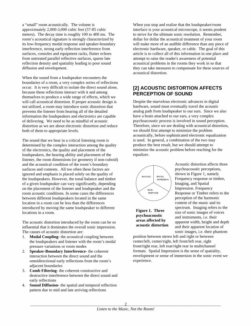
Acoustic distortion affects three psychoacoustic perceptions, shown in Figure 1, namely Frequency response or timbre, Imaging, and Spatial Impression. Frequency Response or Timbre refers to the perception of the harmonic content of the music and its spectrum. Imaging refers to the size of sonic images of voices and instruments, i.e. their apparent width, height and depth and their apparent location of sonic images, i.e. their phantom

position between stereo left and right or between center/left, center/right, left front/left rear, right front/right rear, left rear/right rear in multichannel formats. Spatial Impression is the sense of spatiality, envelopment or sense of immersion in the sonic event we experience.

BASS

RESPONSE

SPATIAL

IMPRESSION

IMAGING

Figure 1. Three psychoacoustic areas affected by acoustic distortion


3

[3] HEARING IS BELIEVING

Acoustic Distortion is difficult to describe. Hearing is believing! Some of the effects we describe can be simulated using hardware that recording engineers typically have on hand. In Figure 2 we describe an equivalent circuit for acoustical distortion. The signal from a DAW or mixer is fed to a parametric or graphic equalizer, then to a digital delay unit and finally to an amplifier and loudspeaker. Wouldn’t it be a rather bad trick to secretly insert this circuit in the signal path prior to a critical mix? The circuit would boost 71, 142, 213 Hz by 10 dB, and introduce 4ms, 7 ms, 9 and 10 ms of delay. The engineer would mix the sound product and subconsciously attempt to adjust for these effects. Imagine the surprise when they were informed of this dirty deed and they played back the mix with the equalizer and digital delay switched off! This is not a practical joke, because the room is playing this trick on engineers all the time. Everything you record and mix is being “heard’ through the “lens” of the room. It’s like looking at the world wearing “rose colored” glasses. You are listening to your music wearing “room colored” ear muffs.

��

��

��

��

��

Figure 2. Equivalent circuit for acoustical distortion


4

[4] SOURCES OF ACOUSTIC DISTORTION

[4.1] Room Modes

All mechanical systems have natural resonances. These resonances are one aspect that differentiates acoustic instruments. In rooms, sound waves coherently interfere as they reflect back and forth between hard walls. This interference results in resonances at frequencies determined by the geometry of the room. In completely reflective rectangular (cuboid) rooms, where the normal component of the particle velocity is zero at the surface, the modal frequencies, associated with the eigenvalues of the wave equation, fn n nx y z

, are determined by Eq. 1.

fc n

L

n

L

n

Ln n nx

x

y

y

z

zx y z

2

2 2 2

(1)

nx, ny and nz are non-negative integers, Lx, Ly and Lz are the length, width and height of the room and c is the speed of sound. These modal frequencies are distributed among axial modes involving two opposing surfaces (e.g. nx=1, ny=0, nz=0), tangential modes involving 4 surfaces (e.g. nx=1, ny=1, nz=0), and oblique modes involving all surfaces (e.g. nx=1, ny=1, nz=1).

For an axial mode between two opposite boundaries, this frequency is equal to the speed of sound, c, divided by twice the room dimension in that direction. For example, for c = 1,130 ft/sec, a 15’ wall to wall dimension results in a first-order fundamental room mode of 37.6 Hz. As an example, in Figure 3 we present the measured modal frequency response of a room whose length is 15’. The loudspeaker was located in a corner and the

microphone was placed against a wall perpendicular to the 15’ dimension, in order to record all axial modes. The first-order (100), second-order (200) and third-order (300) modes are identified in Figure 3 at 37.6 Hz, 75.3 Hz and 113 Hz, respectively. Notice the (100) mode has one nodal plane, the (200) has two and the (300) has three perpendicular to the 15’ length x-axis. As the frequency increases, room modes are still present, but their number and density increase and are not perceived as a problem. Each of these modal frequencies has an associated 3-dimensional pressure distribution in the room. In Figure 4 we present a 2-dimensional illustration of the pressure distribution perpendicular to the length of the room, which is normalized to one. The numbers nx, ny and nz indicate the number of nodal planes of zero sound pressure perpendicular to the x-axis, y-axis and z-axis. In this example, ny and nz are zero and nx takes the value 1, 2 and 3. Thus, in addition to choosing dimensional ratios that uniformly space the modal frequencies, we must consider how the listener and loudspeakers couple with the modal pressures that exist at the locations of the listener and loudspeakers.

0

0.1

0.2

0.3

0.4

0.5

0.6

0.7

0.8

0.9

1

0 0.2 0.4 0.6 0.8 1

Fractional Room Dimension

No

rmal

ized

So

un

d P

ress

ure

Lev

el

First-Order Mode Second-Order Mode Third-Order Mode

Since conventional closed or ported dynamic loudspeakers are pressure sources, they will couple most efficiently when placed at a high pressure region of the modal or sometimes called standing-wave pressure distribution. The loudspeaker placement will accentuate or diminish the coupling with the modal pressure variations at each of the modal frequencies. Similarly, a listener will hear different modal emphasis depending on where he or she is seated. Figure 4 illustrates how the sound energy is distributed along a room dimension. The room dimension is shown as a fraction ranging from 0 to 1. 0.5 would be in the center of the room and 1 would be

Figure 3. Measured modal frequency response in a room 7.5’(W) x 15’ (L) x 9’ (H). The (100), (200), and (300) modes are identified.

Figure 4. Normalized energy distribution of the first three modes in a room.

(100) (200) (300)


5

against a wall. Examining Figure 4 reveals that the fundamental has no energy in the center of the room. Physically this means that if you were sitting in the middle of the room you would not hear this frequency. The first harmonic, however, is at a maximum. It can be inferred from this plot that, in the center of the room all odd harmonics are absent and all even harmonics are at a maximum. Sound waves are longitudinal waves. While often pictured as a sinusoidal transverse wave, sound wave actually oscillate (expand and contract) in the direction of propagation. As the sound waves expand and contract they cause high-pressure regions and low-pressure regions. The instantaneous pressure on opposite sides of a pressure minimum has opposite polarity. The pressure on one side is increasing while the pressure on the other side is decreasing. The position of a loudspeaker and listener’s ear with respect to these pressure variations will determine how they couple with the room. [4.1.1] Non-Rectangular Rooms Most project studios are rectangular simply because they are converted bedrooms, offices, garages, etc. Since they are rectangular we can calculate the modal frequencies and pressure distributions. Once they become non-rectangular, none of this simple math applies and we must rely on finite element method (FEM) or boundary element method (BEM) analysis, which we will discuss later. The simple nodal planes become nodal surfaces! FEM and BEM simulations are used extensively in the aerospace, automotive and underwater acoustics communities, but the cost of the programs precludes their every day use in architectural acoustics. At RPG we use a program called SysNoise to carry out FEM/BEM analyses as well as an in-house proprietary code to optimize surface shapes using iterative BEM calculations. In BEM calculations a mesh of the enclosure, consisting of hundreds or thousands of small elements, is created. The element size is typically 1/6 of the upper frequency limit. There exists an equation for each element over which the pressure is assumed constant. These equations are solved for each frequency of interest and the sound pressure level at any observation point can be determined. While this is a horrendous calculation, it is doable for any shape enclosure. The FEM approach determines the eigenmodes and the frequency response is determined by summation of the modes.


6

[4.2] SPEAKER-BOUNDARY INTERFERENCE RESPONSE

Room modes develop as reflected sound interferes with itself. This next type of acoustic distortion is due to the coherent interference between the direct sound of a loudspeaker and the reflections from the room, in particular the corner immediately surrounding it. This distortion occurs across the entire frequency spectrum, but is more significant at low frequencies. We refer to it as the Speaker Boundary Interference Response or SBIR. The room’s boundaries surrounding the loudspeaker mirror the loudspeaker forming virtual images. When these virtual loudspeakers (reflections) combine with the direct sound, they can either enhance or cancel it to varying degrees depending on the phase

relationship between the reflection and direct sound at the listening position. In Figure 5 a loudspeaker is located 3’ from each room surface with coordinates (3,3,3). The four virtual images on opposite sides of the main room boundaries that are responsible for first order reflections are also shown. A virtual image is located an equivalent distance on the opposite side of a room boundary. The distance from a virtual source to the listener is equal to the reflected path from source to listener. In addition to the four virtual images shown, there are 7 more. Three virtual images and 1 real image in the speaker plane and 4 virtual images of these above the ceiling and floor planes. Imagine that the walls are removed and 11 additional physical speakers are located at the virtual image positions. The resultant sound at a listening position would be equivalent to the sound heard from one source and 11 reflections!.

The effect of the coherent interference between the direct sound and these virtual images is illustrated in Figure 6. The SBIR is averaged over all listening positions with the speaker located 4’ from one, two and three walls surrounding the loudspeaker. It can be seen that as each wall is added, the low frequency response increases by 6 dB and the notch, at roughly 100 Hz, gets deeper. It is important to note at this point that once this notch is created, due to poor placement, it is virtually impossible to eliminate without moving the listener and loudspeaker, since it is not good practice to electronically compensate for deep notches. Thus the boundary reflections either enhance or cancel the direct sound depending on the phase relationship between the direct sound and the reflection at the listening position. Initially, the direct sound and reflection are in phase and they add. As the frequency increases the phase of the reflected sound lags the direct sound. At a certain frequency the reflection is out of phase with the direct sound and a cancellation occurs. The extent of the null will be determined by the relative amplitudes of the direct sound and reflection. At low frequencies there is typically very little absorption efficiency on the boundary surfaces and the notches can be between 6 and 25 dB! The conclusion is obvious, never place a speaker’s woofer equidistant from the floor and two surrounding walls. The low frequency rise in Figure 6 illustrates why one can add more bass by moving a loudspeaker into the corner of a room. Actually one has two choices. Either move the loudspeaker as close to the corner as possible or as far away from the corner as is physically practical. As you move the speaker closer into the corner, the first cancellation notch moves to higher frequencies, where it may be attenuated with porous absorption. This can be seen in Figure 6 for the last condition in which the loudspeaker is positioned 1’ from the floor, rear and sidewalls. In addition, the loudspeaker’s own directivity pattern diminishes the backward radiation thus reducing

ORIGIN OF SOUND SOURCE(3,3,3)

(3,-3,3)VIRTUAL IMAGE

(3,3,14)VIRTUAL IMAGE

(-3,3,3)VIRTUAL IMAGE

(3,3,-3)VIRTUAL IMAGE

CEILING

WALL

FLOOR

Figure 5. Sound from real and virtual speakers combine to create the speaker/boundary interference response.

-25

-20

-15

-10

-5

0

5

10

15

20

0 200 400 600 800 1000

Frequency, Hz

Pre

ssur

e, d

B

1 Boundary X=4'

2 Boundaries X=4', Y=4'

3 Boundaries X=4', Y=4', Z=4'

3 Boundaries X=1', Y=1', Z=1'

Figure 6. Speaker-Boundary Interference Response for several loudspeaker positions near a corner.


7

the amplitude of the reflection relative to the direct sound. This principle is the basis for flush mounting loudspeakers in a corner soffit. The bad news is that with the loudspeaker in the wall-wall dihedral or wall-wall-ceiling trihedral corner, the loudspeaker very efficiently couples with the room modes. If the dimensional ratios are poor leading to overlapping or very widely spaced modal frequencies there will be significant modal emphasis. Professional loudspeaker manufacturers usually provide the low frequency roll off equalization to compensate for the added emphasis of flush mounting the speaker. We can also move the loudspeaker farther away from the adjacent corner. In this case the first cancellation notch moves to lower frequency, hopefully below the lower cutoff frequency of the loudspeaker or the hearing response of the listener. To obtain a 20 Hz first cancellation notch one needs to position the loudspeaker 14’ from the rear wall! Clearly, some happy medium needs to be found and with the myriad alternatives available the most effective approach is to start with a multi-dimensional computer optimization (described later) and tweet to taste.


8

[4.3] Comb Filtering

Another form of acoustic distortion introduced by room reflections is comb filtering. It is due to interference between the direct sound and a reflected sound. In critical listening rooms, we are primarily concerned with the interaction between the direct sound and the first-order (i.e. single-bounce) reflections. Reflections cause time delays, because the reflected path length between the listener and source is longer than the direct sound path.

-20

-15

-10

-5

0

5

10

0 500 1000 1500 2000 2500 3000

Frequency, Hz

Leve

l, dB

0 dB

3 db6 dB

12 dB

Thus when the direct sound is combined with the reflected sound, we experience notches and peaks referred to as comb filtering. The reflections enhance or cancel the direct sound to varying degrees depending on the phase (path length) difference the reflection and the direct sound at the listening position. An example of comb

Figure 7. Comb filtering with 1 one reflection delayed by 1 ms with attenuated of 0, 3, 6 and 12 dB relative to the direct sound.

Figure 8. Comb filter destructive interference null frequencies for a single reflection delayed 1 ms from the direct sound. Constructive interference peaks occur midway between adjacent nulls.

Figure 9. Comb filter due to equi-spaced flutter echoes 1 ms apart.

Reflection Control

Direct Sound Only

Figure 10. Time and frequency response of the direct sound from a loudspeaker.


9

10

100

1000

10000

100000

0.1 1 10 100

Total Delay, Feet

Fre

qu

en

cy, H

z

First NullSecond NullThird NullFourth NullFifth Null

-6

-4

-2

0

2

4

6

8

10

12

0 500 1000 1500 2000 2500 3000

Frequency, Hz

Leve

l, dB

filtering between the direct sound and a reflection delayed

by 1 ms is shown in Figure 7. Four conditions are illustrated. 0 dB refers to the theoretical situation in which the reflection is at the same level as the direct sound. The remaining three interference curves indicate situations in which the reflection is attenuated by 3, 6 and 12 dB. In Figure 8 the locations of the first 5 interference nulls are indicated as a function of total delay. A delay of 1 ms or 1.13’ produces a first null at 500 Hz with subsequent notches 1000 Hz apart. The constructive interference peaks lie midway between successive nulls. When the reflection is at the same level as the direct sound the nulls theoretically extend to infinity. This name evolved, because comb filtering resembles a series of equally spaced notches like the teeth of a comb. The location of the first notch is given by the speed of sound divided by 2 times the total path length difference. The spacing between subsequent notches is twice this frequency. In Figure 9 the comb filtering due to a series of regularly spaced reflections separated by 1 ms (flutter echo) is shown. Note how the peaks are much sharper than the single reflection. The audible effect of comb filtering is easy to experience using a delay line. If you combine a signal with a delayed version, you will experience various effects referred to as chorusing or flanging, depending on the length of the delay and the variation of the delay with time. Shorter delays have wider bandwidth notches and thus remove more power than longer delays. This is why microsecond and millisecond delays are so audible. The effect of a reflection is illustrated in Figure 10 and Figure 11. In Figure 10 we illustrate the time and frequency responses from the right speaker only. The upper curve shows the arrival time and the lower curve shows the free-field response of the loudspeaker. In Figure 11 we show the effect of adding a side wall reflection to the sound of the right speaker. The upper curve shows the arrival time of both the direct sound and the reflected sound. The lower curve shows the severe comb filtering that a single reflection introduces. If your speaker had a free-field response like this lower curve, you probably would not have purchases it. Yet, many rooms are designed without reflection control. In reality our ear/brain combination is more adept at interpreting the direct sound and reflection than the FFT analyzer, so that the effect may be somewhat less severe. Comb filtering is controlled by attenuating the room reflections or by controlling the loudspeaker’s directivity to minimize boundary reflections. If the loudspeaker has constant directivity as a function of frequency, then broad bandwidth reflection control is necessary. Since the directivity of conventional loudspeakers increases with frequency, low frequency reflection control is important. For this reason, one would not expect to control low frequency comb filtering effects with a thin porous acoustical foam or panel.

Reflection Control

Direct Sound &1st Reflection

Figure 11. Time and frequency response of the direct sound combined with a side wall reflection. The comb filtering is apparent


10

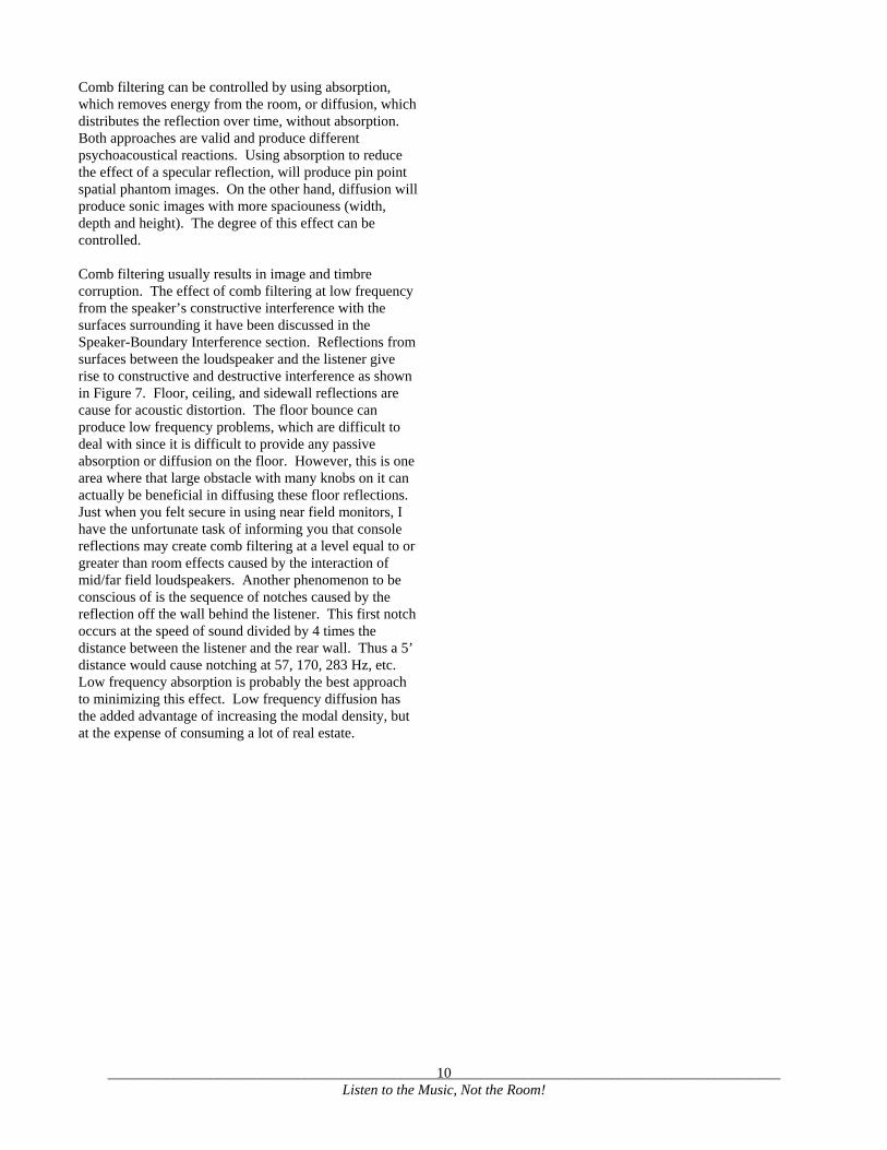
Comb filtering can be controlled by using absorption, which removes energy from the room, or diffusion, which distributes the reflection over time, without absorption. Both approaches are valid and produce different psychoacoustical reactions. Using absorption to reduce the effect of a specular reflection, will produce pin point spatial phantom images. On the other hand, diffusion will produce sonic images with more spaciouness (width, depth and height). The degree of this effect can be controlled. Comb filtering usually results in image and timbre corruption. The effect of comb filtering at low frequency from the speaker’s constructive interference with the surfaces surrounding it have been discussed in the Speaker-Boundary Interference section. Reflections from surfaces between the loudspeaker and the listener give rise to constructive and destructive interference as shown in Figure 7. Floor, ceiling, and sidewall reflections are cause for acoustic distortion. The floor bounce can produce low frequency problems, which are difficult to deal with since it is difficult to provide any passive absorption or diffusion on the floor. However, this is one area where that large obstacle with many knobs on it can actually be beneficial in diffusing these floor reflections. Just when you felt secure in using near field monitors, I have the unfortunate task of informing you that console reflections may create comb filtering at a level equal to or greater than room effects caused by the interaction of mid/far field loudspeakers. Another phenomenon to be conscious of is the sequence of notches caused by the reflection off the wall behind the listener. This first notch occurs at the speed of sound divided by 4 times the distance between the listener and the rear wall. Thus a 5’ distance would cause notching at 57, 170, 283 Hz, etc. Low frequency absorption is probably the best approach to minimizing this effect. Low frequency diffusion has the added advantage of increasing the modal density, but at the expense of consuming a lot of real estate.


11

[5] ACOUSTICAL SOLUTIONS

We now discuss some practical solutions. Since real world limitations have a nasty habit of getting in the way of our beautifully conceived mathematical models, we will also mention the limitations of these suggestions. We can think of a tool kit of Bass Tools to improve bass response, Imaging Tools to control imaging and Spatial Tools to improve sound diffusion and our sense of envelopment.

[5.1] Bass Tools

The perceived bass response in a room is controlled by the free-field loudspeaker response, the room dimensions, the acoustic coupling of the listener/loudspeakers to the modal pressure variations, the speaker-boundary interference between the direct sound and adjacent reflections, the internal contents of the room, the acoustical nature of the boundary surfaces and surface treatment and the hearing response and training of the listener. Any absorption or amplification over a frequency range, which is introduced by the room, will color the sound that we hear. The room will thus introduce its own signature rather than having a flat frequency response. Since most of today’s speakers are of high quality and we may not have any control over the room's dimensions, we can focus our attention on proper speaker placement and acoustical treatment. Proper speaker placement can optimize the coupling with the room’s standing wave pattern and the interference between the speaker and reflected sounds from the nearby corner. This can result in severe cancellations if the speaker is located an equal distance from all boundaries. After locating the speakers (and the listener) properly, we may choose to utilize low frequency absorbers to damp room resonances and minimize the speaker/boundary interference. Following all of this you may want to fine-tune the bass response using electronic equalization. [5.1.1] Room Dimensions If one is building a new room, it is useful to consider dimensional ratios. One might wonder if there is an ideal room. As usual the answer is yes and no. If the room is rectangular there are various approaches to choose dimensional ratios that uniformly distribute the modal frequencies. One of these determinations by Louden, illustrated in Table 1, yields the following dimensional ratios in order of preference. As an example, a room with

a 10’ ceiling height would have a 14’ width and a 19’ length. At RPG we have also developed an automated algorithm to minimize the standard deviation of the modal pressure response, which may also prove helpful.

Table 1. Room dimensions in order of preference according to Louden.

ORDER LENGTH WIDTH 1 1.9 1.4 2 1.9 1.3 3 1.5 2.1 4 1.5 2.2 5 1.2 1.5 6 1.4 2.1 7 1.1 1.4 8 1.8 1.4 9 1.6 2.1 10 1.2 1.4 11 1.6 1.2 12 1.6 2.3 13 1.6 2.2 14 1.8 1.3 15 1.1 1.5 16 1.6 2.4 17 1.6 1.3 18 1.9 1.5 19 1.1 1.6 20 1.3 1.7 Rectangular Modal Prediction Limitations: The modal frequency calculations based on rectangular room dimensions assume that the room is rectangular and that the walls are perfectly reflecting. Real rooms are at times non-rectangular, wall surfaces and windows may absorb low frequencies due to diaphragmatic vibration and also transmit low frequencies, and internal furnishings can scatter and absorb low frequencies. These effects will cause an error in the calculated modal frequencies. At low frequencies small perturbations, like alcoves and soffits, which are small compared to the long wavelengths may introduce only small changes. Also any prediction should properly weight the axial, tangential and oblique modes in this order. Another thing that is assumed is perfect acoustical coupling between sources and modes, in which all modes are uniformly energized. The actual locations for loudspeakers may only energize a subset of the modes and the listeners may be in locations, which do not permit them to hear the effects of even those modes that are excited. One might wonder if making a room non-rectangular is a benefit. The first thing to understand is that making the room non-rectangular does not make modes disappear and does not make the modal behavior less pronounced than in an equivalent rectangular room, just different.

BASSTOOLS

SPATIALTOOLS

IMAGINGTOOLS

Figure 12. Acoustic tools improve imaging, spaciousness and bass response.


12

The magnitudes in the pressure variations do not vary substantially, but the changes in frequency distribution and nodal lines are non-intuitive. Splaying of sidewalls or ceiling to reduce high frequency flutter effects, has minimal effect on modal problems and the mid-dimension of the tapered wall may be used for rectangular analysis. Beneficial low frequency modal mixing leading to increased diffusion may be introduced even by making one wall non-rectangular. However, one should have an acoustician carry out FEM calculation to verify performance to insure the effort is producing a beneficial and useful effect, since non-rectangular construction is often more expensive and introduces non-symmetric effects, which may affect imaging. BEM/FEM Limitations: The limitation of these approaches is that the acoustical properties of the enclosure must be precisely known. At low frequencies many structures exhibit panel or Helmholtz resonances, with associated large changes in impedance, over small frequency ranges. Data for the acoustic properties (complex impedance) of commonly used structural and decorative materials are not available. Data may be obtained from impedance tube testing, but this too may lead to errors because samples cannot be tested at full scale. Once these data become more widely available progress in non-rectangular room predictions may play a more active role in architectural acoustics. [5.1.2] Optimize Location of the Listener and Loudspeakers Since the modal coupling and speaker-boundary interference are position related, optimizing these effects seems like a good way to start. Especially, since they involve a cost-free remedy. One could start by placing the loudspeakers in a given location and listening to the response. Then moving the loudspeakers and listener locations in a systematic trial and error manner until a satisfactory response is achieved. This may be practical for mono, or maybe even stereo, if you have enough patience and your monitors are not extremely heavy, but for multichannel 5.1 digital formats, this may prove impractical. At RPG we considered ways of letting the computer do the moving! We can describe the necessary steps by the acronym DESIRE. Describe- How do we mathematically describe the system? To accomplish this one needs to be able to predict the room response at hundreds or maybe thousands of listener/loudspeaker locations. For rectangular rooms, which fortunately model many project studios, one can accurately calculate the room response for a given listener/loudspeaker location using either the mode summation method or by a reflection summation

method and Fourier transforming the resulting room’s impulse response. Mode Summation Method- The pressure at the listening position from a group of loudspeakers in a rectangular room can be modeled by a rather complex expression of six cosine terms containing the integer mode identification and room dimensions, the damping factors of the modes, etc. The calculation is time intensive and care must be taken to include all of the modal frequencies contributing in the frequency range of interest, plus corrections for those modes lying outside this range. This system description is available for use in the program. Reflection Summation Method- Since we will be evaluating many possibilities, the equivalent reflection summation impulse response approach using an image model is more efficient and is the default approach used in the program. The image model includes only those images contributing to the impulse response and provides appropriate weighting of the contribution of each mode. It has the advantage that it is a transient calculation, in which one could use any desired amount of time. It offers the additional benefit that having determined the impulse response by following the reflection history of rays reflected around the room, we could extract the effects of the speaker-boundary interference from the early time portion and the modal response from the entire time history. Since modes can only exist if reflections are specularly reflected over many orders. You may wonder how the surfaces of a relatively small room can produce low-frequency specular reflection, when the wavelengths associated with low frequencies are larger or comparable with the extent of the boundary surfaces. In a free field a wall of say 10’ would produce diffusion at 113 Hz, which has a wavelength of 11.3’. However, in a rectangular room, the virtual images as described in the SBIR section, effectively extend the boundary extent to infinity. Thus a rectangular room acoustically consists of three sets of intersecting infinite planes. Boundary absorption may practically reduce the extent of these planes, but the effective reflection is specular even though the physical surfaces are small. Evaluate- How do we evaluate the calculated performance? Once the speaker-boundary and modal responses are calculated, we must theoretically evaluate them. We must find a parameter that corresponds to what we might say if we were actually listening to this trial location. To accomplish this we adopted the flatness of the room’s frequency response as a predictor. This was selected based on the extensive work of Floyd Toole and his associates in determining the importance of a flat and smooth loudspeaker response on listener preference. To


13

evaluate the quality of the listener/loudspeaker locations, we sum the standard deviation of the room response determined from a cosine squared windowed FFT of the first 65 ms of the impulse response and the standard deviation of the entire impulse response. The standard deviation has proven to be a reliable statistical indicator of deviations from a mean response. Therefore, we can now let the computer do the moving, by automatically evaluating as many trial listener/loudspeaker locations as is necessary to produce a satisfactory room response. Search- How do we search the millions of possible trial locations? Out of the millions of possible locations for the listener and loudspeakers, how do we automatically decide which trial locations to evaluate next. Fortunately, mathematicians have examined this problem and developed intelligent search engines. These algorithms learn as they go and hence find the optimum trajectory through the error space using multi-dimensional simplex minimization. IteRate- How do we automate this trial and error optimization cycle? We then need to set up a cyclical iteration path in which the impulse response for new trial locations are determined, room response calculated, standard deviation determined and a comparison between desired quality and current quality is made. If the quality is acceptable the program ends. If not another set of trial locations is determined and evaluated. This is accomplished using a simple If check. End- How do we know when we are done? We now need a way to tell the computer it is finished. This is accomplished by storing the weighted standard deviations for each trial position of listener and loudspeakers. When further movement does not produce any further benefit or if the number of iterations exceeds a certain number the program ends. In 1997, we put all of this together and published the first algorithm to simultaneously minimize the effect of the modal coupling and the speaker-boundary interference using an image model and multi-dimensional optimization techniques. The program allows a fast evaluation of a very large number of possible listener and loudspeaker locations. It also indicates the first order reflection coordinates for application of mid/high frequency surface treatment to address imaging issues. We thus have a method to optimize the placement of the listener and loudspeakers, within physically accessible or desirable regions of the listener and loudspeakers for any number and type of loudspeakers. The Speaker-Boundary Interference Response improvement between the worst locations found for the listener and loudspeaker is shown in Figure 13. The improvement in the modal responses

between the worst and best locations of listener and loudspeaker is shown in Figure 14.

50

60

70

80

90

100

0 50 100 150 200 250 300

Frequency (Hz)

Le

vel (

dB

Best case

Worst case

Figure 13. Speaker-Boundary Interference The standard deviations are 4.67 and 8.13 dB for the best solution and worst case respectively.

50

60

70

80

90

0 50 100 150 200 250 300

Frequency (Hz)

Le

vel (

dB

Best case

Worst case

Figure 14. Modal Response- The standard deviations are 3.81 and 6.28 dB for the best solution and worst case, respectively Real World Limitations- Real rooms may not be perfectly rectangular, they may be large bulky obstacles with lots of knobs in the room, like a console, walls may not be perfectly reflective (like one layer of drywall), there may be windows, etc. At low frequencies, the wavelengths are very long (50 Hz being 22.6’) that small perturbations are not “seen” and the principal dimensions may be satisfactory to describe the room. In light of all of this, the multi-dimensional optimization should be regarded as a fast way to get close and it is always advisable to measure the room using impulses, swept sine waves, maximum length sequences or transfer function approaches. No directivity information is used for sources, but this is not a serious


14

limitation as woofers operating below 200-300 Hz are omnidirectional. [5.1.3] Sub-Woofer So far we have discussed optimizing the location of the woofers to find the best acoustical coupling with the room’s modal pressure variations and speaker-boundary interference. While improving the bass response by locating full range loudspeakers, there is the obvious chance to adversely affect the higher frequency effects of imaging. There may be occasions where a choice has to be made, since both may not be achievable simultaneously. A convincing arguments for the use of one or more separate sub-woofers is that they offer the opportunity to achieve good bass response by locating the sub-woofer independently of the mid/high frequency loudspeakers. Multiple sub-woofers also offer the opportunity to increase modal mixing as well as offer low frequency spatial effects, which some argue are not perceivable. Optimum sub-woofer locations are achievable by physical trial and error or by multi-dimensional analysis. The obvious place to start is in the corner, since the sub-woofer couples so efficiently in this location. The potential problem with this location is that all of the modes will be excited and if the dimensional ratios are poor, this location will lead to severe low-frequency coloration. It’s best to predict the optimum performance and then let your ears be the judge. [5.1.4] Damp the Modes One method to reduce the magnitude of these effects is to increase the damping factors of all of the modes by suitable use of low frequency absorptive materials. By increasing the damping factor, the maximum amplitude of the resonance is reduced and the range of frequencies over which it acts is widened. Most people are familiar with acoustical foam or other porous absorbers, which absorb sound by converting sound energy into heat. The efficiency of a porous absorber is highest when the sound is traveling at its highest velocity. This point is reached at ¼ of the wavelength and thus varies with the frequency. At low frequencies like 100 Hz, this distance is about 2.5’ from the wall. Unfortunately at the wall surface where the porous absorber is usually placed, the particle velocity is zero. This is where the sound wave changes direction on reflection and hence the velocity is zero. Since porous absorbers rely on particle velocity, they have limited efficiency at low frequencies. The point to be taken away from this discussion is that placing porous absorbers on a wall or in a corner is pointless. Fortunately, there is another mechanism that can be utilized. At the wall the particle velocity is zero, but the pressure is a maximum. To exploit this phenomenon, on can employ a membrane with high internal losses and an air cavity with a porous material near the membrane. The membrane can be tuned to sympathetically oscillate with

the pressure fluctuations at low frequency, thus creating air movement through the internal porous material. These

0

0.2

0.4

0.6

0.8

1

1.2

10 100 1000

Frequency, Hz

Abs

orpt

ion

Coe

ffic

ient

BASS Trap

Figure 15. Low frequency membrane absorber response

Devices are called membrane absorbers and a typical absorption coefficient response is shown in Figure 15. Another approach to essentially create particle velocity is to make use of the pressure gradient between the inside and outside of a volume enclosed by a porous material. Another newly modeled mechanism is the pressure gradient absorption produced by reflection phase grating diffusors. When the pressure difference between adjacent wells, separated by dividers, equilibrates significantly increased particle velocities over the dividers introduces low frequency absorption below the design frequency. Another approach is to use Helmholtz absorbers, which consist of a series of slots or holes in a panel placed over an air cavity with a porous material close to, but not touching, the panel. New theoretical models for neck designs holds promise to increase the bandwidth of these new devices. [5.1.5] Electronic Equalization In a small project studio the listener is typically located in the direct field within the critical distance (that point at which the direct and reverberant sound are at the same level). In this case, full bandwidth electronic equalization to compensate for room problems should be avoided as it would corrupt the one thing that may be acceptable in the room, namely the frequency response of the direct sound! Therefore, prudence dictates that mid/high frequency equalization or time domain filtering be used by a trained acoustician. On the other hand, there may be valid reasons to introduce low frequency electronic equalization to complete the adjustment of the low frequency room response. Psychoacoustically, the effect of room modes on the effective output power of the loudspeaker is essentially indistinguishable from a real departure of the loudspeaker from a level response. Low frequency


15

equalization below roughly 300 Hz is justifiable when, for practical reasons, one cannot relocate the listening position or loudspeaker positions or to fine tune the room’s low frequency response. Low Frequency Limitations Attenuation of excess peaks is acceptable, but one should avoid trying to raise the level of notches. Response notches are usually the result of nulls in the modal response or destructive interference. Therefore, their extent may be limitless. Thus any gain introduced to compensate will reduce the amplifier headroom and increase distortion. When making corrections based on acoustical measurements, spatial averaging is prudent to not only help identify the source of the problem, but allow for practical movement.

[5.2] Image Tools

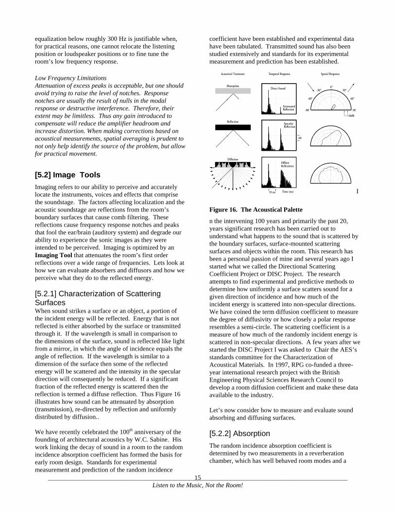
Imaging refers to our ability to perceive and accurately locate the instruments, voices and effects that comprise the soundstage. The factors affecting localization and the acoustic soundstage are reflections from the room’s boundary surfaces that cause comb filtering. These reflections cause frequency response notches and peaks that fool the ear/brain (auditory system) and degrade our ability to experience the sonic images as they were intended to be perceived. Imaging is optimized by an Imaging Tool that attenuates the room’s first order reflections over a wide range of frequencies. Lets look at how we can evaluate absorbers and diffusors and how we perceive what they do to the reflected energy. [5.2.1] Characterization of Scattering Surfaces When sound strikes a surface or an object, a portion of the incident energy will be reflected. Energy that is not reflected is either absorbed by the surface or transmitted through it. If the wavelength is small in comparison to the dimensions of the surface, sound is reflected like light from a mirror, in which the angle of incidence equals the angle of reflection. If the wavelength is similar to a dimension of the surface then some of the reflected energy will be scattered and the intensity in the specular direction will consequently be reduced. If a significant fraction of the reflected energy is scattered then the reflection is termed a diffuse reflection. Thus Figure 16 illustrates how sound can be attenuated by absorption (transmission), re-directed by reflection and uniformly distributed by diffusion.. We have recently celebrated the 100th anniversary of the founding of architectural acoustics by W.C. Sabine. His work linking the decay of sound in a room to the random incidence absorption coefficient has formed the basis for early room design. Standards for experimental measurement and prediction of the random incidence

coefficient have been established and experimental data have been tabulated. Transmitted sound has also been studied extensively and standards for its experimental measurement and prediction has been established.

I

n the intervening 100 years and primarily the past 20, years significant research has been carried out to understand what happens to the sound that is scattered by the boundary surfaces, surface-mounted scattering surfaces and objects within the room. This research has been a personal passion of mine and several years ago I started what we called the Directional Scattering Coefficient Project or DISC Project. The research attempts to find experimental and predictive methods to determine how uniformly a surface scatters sound for a given direction of incidence and how much of the incident energy is scattered into non-specular directions. We have coined the term diffusion coefficient to measure the degree of diffusivity or how closely a polar response resembles a semi-circle. The scattering coefficient is a measure of how much of the randomly incident energy is scattered in non-specular directions. A few years after we started the DISC Project I was asked to Chair the AES’s standards committee for the Characterization of Acoustical Materials. In 1997, RPG co-funded a three-year international research project with the British Engineering Physical Sciences Research Council to develop a room diffusion coefficient and make these data available to the industry. Let’s now consider how to measure and evaluate sound absorbing and diffusing surfaces. [5.2.2] Absorption

The random incidence absorption coefficient is determined by two measurements in a reverberation chamber, which has well behaved room modes and a

Figure 16. The Acoustical Palette


16

well-characterized reverberation time versus frequency. After

100125

160200

250315

400500

625800

10001250

16002000

25003150

4000

Frequency, Hz

0

0.2

0.4

0.6

0.8

1

Ab

sorp

tio

n C

oef

fici

ent

Legend1" Absorber Spaced From Wall1" Absorber mounted on wall

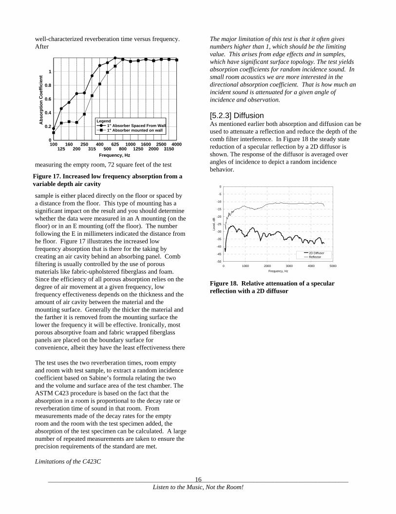
measuring the empty room, 72 square feet of the test

sample is either placed directly on the floor or spaced by a distance from the floor. This type of mounting has a significant impact on the result and you should determine whether the data were measured in an A mounting (on the floor) or in an E mounting (off the floor). The number following the E in millimeters indicated the distance from he floor. Figure 17 illustrates the increased low frequency absorption that is there for the taking by creating an air cavity behind an absorbing panel. Comb filtering is usually controlled by the use of porous materials like fabric-upholstered fiberglass and foam. Since the efficiency of all porous absorption relies on the degree of air movement at a given frequency, low frequency effectiveness depends on the thickness and the amount of air cavity between the material and the mounting surface. Generally the thicker the material and the farther it is removed from the mounting surface the lower the frequency it will be effective. Ironically, most porous absorptive foam and fabric wrapped fiberglass panels are placed on the boundary surface for convenience, albeit they have the least effectiveness there The test uses the two reverberation times, room empty and room with test sample, to extract a random incidence coefficient based on Sabine’s formula relating the two and the volume and surface area of the test chamber. The ASTM C423 procedure is based on the fact that the absorption in a room is proportional to the decay rate or reverberation time of sound in that room. From measurements made of the decay rates for the empty room and the room with the test specimen added, the absorption of the test specimen can be calculated. A large number of repeated measurements are taken to ensure the precision requirements of the standard are met. Limitations of the C423C

The major limitation of this test is that it often gives numbers higher than 1, which should be the limiting value. This arises from edge effects and in samples, which have significant surface topology. The test yields absorption coefficients for random incidence sound. In small room acoustics we are more interested in the directional absorption coefficient. That is how much an incident sound is attenuated for a given angle of incidence and observation. [5.2.3] Diffusion As mentioned earlier both absorption and diffusion can be used to attenuate a reflection and reduce the depth of the comb filter interference. In Figure 18 the steady state reduction of a specular reflection by a 2D diffusor is shown. The response of the diffusor is averaged over angles of incidence to depict a random incidence behavior.

-50

-45

-40

-35

-30

-25

-20

-15

-10

-5

0

0 1000 2000 3000 4000 5000

Frequency, Hz

Leve

l, dB

2D DiffusorReflector

Figure 18. Relative attenuation of a specular reflection with a 2D diffusor

Figure 17. Increased low frequency absorption from a variable depth air cavity


17

In Figure 19 we compare the extent of comb filtering between a direct sound and a strong specular reflection and between the direct sound and a diffuse reflection. Note that the diffuse energy is distributed over time and consequently it decreases the depth of the comb filtering, introducing, instead a dense pattern of irregularly spaces frequency notches characteristic of a diffuse sound field.

Figure 19. Diffusive attenuation of specular reflection and accompanying comb filtering.


18

[5.3] Spatial Tools

Diffusing surfaces have been used since antiquity in the form of statuary, coffered ceilings, columns and surface ornamentation. In 1983 RPG introduced the first designable diffusor based on mathematical number theory and tens of thousands of diffusors have been used in the music industry since then. Since they have become so widely used it is important to know how to evaluate a potential diffusor. The method that is being evaluated as a standard is to automatically measure, under computer control, the scattered impulse responses 5 meters from a test surface at an angular resolution of 5 degrees, with the test source at a given angle with respect to the normal and 10 meters away. An illustration of the test geometry is shown in Figure 20. Once the impulse responses are

determined they are Fourier transformed to obtain frequency responses at each observation angle. From these data one can take a frequency slice averaged over 1/3-octave to obtain the polar or angular response. The diffusion spectrum is then defined by a plot of the

standard deviation of the 1/3-octave angular response in dB plotted versus frequency. The diffusion coefficient is obtained by normalizing this curve from 0 to 1 by the scattering from an ideal polar response consisting of a delta function. In Figure 21 we see a plot of the diffusion coefficient of a 2’ x 2’ diffusing surface plotted versus a flat panel of similar size. There are two mechanisms for sound diffusion- size diffraction and surface topology. You will notice that at about 565 Hz the two curves begin to deviate. This is a reality check on the experiment because size diffraction should end at a frequency roughly equal to the speed of sound divided by the size of the panel (1,130 ft/sec/ 2’= 565 Hz). As you can see up to 565 Hz scattering from a flat panel and a diffusor of similar size are equal as it should be. Above this frequency the wavelengths are small enough to “see” the surface variation and begin to diffuse based on the nature of the surface topology. It is important to indicate that not any surface variation is acceptable. Diffusion involves constructive and destructive interference and this complex interaction is often non-intuitive. One of the promising aspects of this approach is that the diffusion performance can also be predicted using BEM calculations In the coming years you will be hearing more and more about modeling using geometrical computer modeling programs. They have been reserved for larger rooms, but inclusion of diffusion algorithms and phase triangular beam tracing has made them more applicable to small rooms like project studios. The missing parameter in this type of modeling is a random incidence diffusion coefficient. As part of our research program we are evaluating a method suggested by Mommertz to measure this quantity directly. This method is very much like the

random incidence absorption coefficient approach, except it uses a maximum length sequence stimulus instead of pulsed noise bursts and an additional measurement is required. Thus one measures the reverberation time of the chamber empty, with the scattering sample stationary and

MICROPHONE(19TYP.)

SAMPLE

MIC BOOM

LOUDSPEAKER TRACKLOUDSPEAKER @ 45°

PLAN VIEW

ELEVATION

DIRECTION OF ROTATION

Figure 20. Measurement Goniometer to map the backscattered hemisphere.

Figure 21. Diffusion coefficient for a 2D diffusor

Figure 22. Scattering coefficient for a quadratic residue diffusor

0

0.1

0.2

0.3

0.4

0.5

0.6

0.7

0.8

0.9

1

125

160

200

250

315

400

500

630

800

1000

1250

1600

2000

2500

3200

4000

Frequency, Hz

Diff

usio

n C

oeff

icie

nt

Diffusor

Reflector

Diffraction LimitWidth =

0

0.2

0.4

0.6

0.8

1

1.2

100 1000 10000

Frequency, Hz

Sca

tterin

g C

oeffi

cien

t


19

with the sample rotating. Rotation removes the incoherent scattering arising from the surface topology and yields only the specular scattering. Thus one can obtain the fraction of the sound scattered in the specular direction. From this and the total sound power, one can obtain the random incidence absorption coefficient, and the scattering coefficient, . In Figure 22 we show the first measurements on a number theoretic diffusing surface showing its random incidence diffusion and absorption spectra.

The type of spatial scattering a diffusing surface offers depends on whether the phase variation occurs in one or two dimensions. A 1-dimensional diffusor is formed from extruding an optimized diffusing profile. The phase variation occurs in only one direction, the direction of the profile, and the other direction has constant depth. In

Figure 23 we show the hemidisc scattering from a 1D diffusor. When the phase varies in two perpendicular directions the diffusor is called a 2D diffusor and it provides hemispherical scattering. This is illustrated in Figure 24. In 1995 I presented a review paper at the AES in New York on two decades of diffusor design and development. This research began with the seminal research of Manfred Schroeder and has progressed from simple number theory quadratic residue diffusors, to diffusing fractals, additive and multiplicative modulated QRDs, to the present state of the art in which almost any desired shape surface can be acoustically optimized using BEM optimization techniques. Over the past 20 years we have developed the ability to predict, measure, quantify and optimize diffusor performance. Small rooms like project studios require a very efficient surface to diffuse interfering wall reflections and provide a diffuse sound field. For this application diffusors with phase variation in two perpendicular directions is ideal. If the phase variation is calculated properly these 2-dimensional surfaces can scatter sound omnidirectionally for any given angle of incidence.

[6] EXAMPLE

In 1983, RPG introduced two new concepts in control room design, which were extensions of the LEDE design concepts by Don Davis. One involved creation of a temporal reflection free zone (RFZ) by reflecting and/or absorbing first order reflections between the listener and loudspeakers. Since flush mounted loudspeakers were popular at that time, the RFZ also included flush mounted loudspeakers as close to the trihedral corner as was feasible. The sidewalls between the loudspeaker and listener were typically splayed away from the listener in order to deflect energy towards the rear of the room. The addition of broad bandwidth absorption on these splayed surfaces further reduced the scattered sound level at the listening position. Recognition of modal excitation with this corner loaded loudspeaker mounting required potential low frequency shelving to the loudspeaker signal. The other idea was to use sound diffusing surfaces on the rear wall to control interfering rear wall reflections, maintain a natural ambiance in the room, widen the sweet spot and create a sense of passive surround sound envelopment. In concert hall research the sense of envelopment was linked to the amount of sound reaching the listener from lateral directions around 55 degrees with respect to the frontal direction. In music reproduction rooms like recording studios, strong lateral reflections would produce comb filtering and corrupt the imaging and timbre of the reproduced sound. The use of sound

Figure 23. Hemidisc scattering from a 1D diffusor

Figure 24. Scattering hemisphere from a 2D diffusor


20

diffusing surfaces on the rear wall helps to acoustically create an impression similar to today’s surround sound systems. We call it “passive surround sound”. Thus we use a Spatial Tool to create envelopment, widen the sweet spot, add warmth and naturalness to the sound, and uniformly distribute the sound throughout the room. The RFZ/RPG design quickly became a sort of defacto standard and photos of this approach are commonplace in trade magazines.

Figure 25 illustrates the results of applying Image and Spatial tools to an untreated room. The display at the top illustrates strong corrupting early reflections from the sidewalls, floor and ceiling between the loudspeakers and the listening position. In addition, reflections arriving

after the rear wall reflection are sparse and do not follow a linear decay as would be found in a diffuse field. The RFZ/RPG design quickly became a sort of defacto standard and photos of this approach are commonplace in trade magazines. Imaging Tools, in the form of broad bandwidth absorption were used to minimize the corrupting early reflections and a temporal Reflection Free Zone 24 dB below the direct sound was created to improve imaging and timbre. Then diffusion was added to the rear wall to minimize the corrupting effect of isolated strong reflections and provide a spatially and temporally dense reflection pattern. Note the linear envelope decay of the diffuse reflections indicative of a diffuse sound field.

[7] SUMMARY

Today project studios are primarily using small freestanding powered monitors and subwoofers. In addition, the rooms are usually approximately rectangular. We can summarize ten steps to help create accurate listening rooms that provide a transferable audio product. The ultimate goal would be to give recording engineers the confidence that what they hear in their room will transfer to other listening locations. When undertaking an acoustical analysis of a room, consult an acoustician. These professionals have a wealth of experience that they can offer in the early stages that will save you time and money in the long run. Below are Dr. Diffusor’s top ten tips that will help you Listen to The Music, Not the Room!! 1. Listen to your recordings in a variety of listening

environments to convince yourself that the acoustics of the listening room play a vital role in what is heard.

2. If you are building a new room, use good dimensional ratios to provide uniform modal frequency distribution. If the room already exists there is not much you can about this.

3. Design a symmetrical listening environment for good imaging. Place speakers symmetrically and on axis for best response.

4. Locate the sub-woofers, loudspeaker woofers and listening position to optimize the acoustical coupling with the room's pressure variations and speaker-boundary interference. I.e. optimize the bass response. Experiment with positioning the woofer above or below the tweeter for optimal coupling with the room.

5. Minimize first order reflections from the walls, ceiling and floor between the loudspeakers and the listening position using absorption or diffusion. Be conscious of the effect of console reflections and minimize.

Figure 25. Time response comparison of an untreated and acoustically treated room.


21

6. Diffuse rear wall reflections over roughly 60% of the surface area beginning 3' off the finished floor.

7. Provide low-frequency absorption on the rear wall to minimize low frequency cancellation effects.

8. If necessary, damp low frequency modes by applying low frequency absorption at maximum pressure locations like dihedral and trihedral corners.

9. Electronically equalize remaining low frequency modal emphasis. Reconsider equalizing frequency notches in the room response. Consider time domain equalization.

10. Measure the room's time and frequency response at several listening positions using any of the excellent transfer function or stimulus and response approaches. Analyze the results and tweak to taste.


22

TABLE OF FIGURES Figure 1. Three psychoacoustic areas affected by

acoustic distortion ..................................................... 2 Figure 2. Equivalent circuit for acoustical distortion ...... 3 Figure 3. Measured modal frequency response in a room

2.29 m (W) x 4.57 m (L) x 2.74 m (H). The (100), (200), and (300) modes are identified. ...................... 4

Figure 4. Normalized energy distribution of the first three modes in a room. .............................................. 4

Figure 5. Sound from real and virtual speakers combine to create the speaker/boundary interference response.6

Figure 6. Speaker-Boundary Interference Response for several loudspeaker positions in a corner. ................ 6

Figure 7. Comb filtering with 1 one reflection delayed by 1 ms with attenuated of 0, 3, 6 and 12 dB relative to the direct sound. ........................................................ 8

Figure 8. Comb filter destructive interference null frequencies for a single reflection delayed 1 ms from the direct sound. Constructive interference peaks occur midway between adjacent nulls. ..................... 8

Figure 9. Comb filter due to equi-spaced flutter echos 1 ms apart. .................................................................... 8

Figure 10. Time and frequency response of the direct sound from a loudspeaker. ........................................ 8

Figure 11. Time and frequency response of the direct sound combined with a side wall reflection. The comb filtering is apparent ......................................... 9

Figure 12. Acoustic tools improve imaging, spaciousness and bass response. ................................................... 11

Figure 13. Speaker-Bondary Interference The standard deviations are 4.67 and 8.13 dB for the best solution and worst case respectively..................................... 13

Figure 14. Modal Response- The standard deviations are 3.81 and 6.28 dB for the best solution and worst case, respectively .................................................... 13

Figure 15. Low frequency membrane absorber response14 Figure 16. The Acoustical Palette .................................. 15 Figure 17. Increased low frequency absorption from a

variable depth air cavity .......................................... 16 Figure 18. Relative attenuation of a specular reflection

with a 2D diffusor ................................................... 16 Figure 19. Diffusive attenuation of specular reflection

and accompanying comb filtering. .......................... 17 Figure 20. Measurement Goniometer to map the

backscattered hemisphere. ...................................... 18 Figure 21. Diffusion coefficient for a 2D diffusor ........ 18 Figure 22. Scattering coefficient for a quadratic residue

diffusor.................................................................... 18 Figure 23. Hemidisc scattering from a 1D diffusor ....... 19 Figure 24. Scattering hemi-shpere from a 2D diffusor .. 19 Figure 25. Time response comparison of an untreated

and acoustically treated room. ................................ 20

Documents

Docs-Technology-White Papers-Minimizing Acoustical Distortion in Project Studios