Docker Overlay Networks - OS3 · Docker Overlay Networks Performance analysis in high-latency environments MSc Research Project ... Socketplane and Calico as viable options. However,

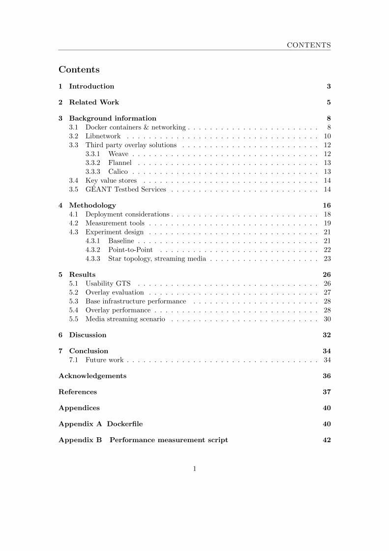
Docker Overlay NetworksPerformance analysis in high-latency environments

MSc Research ProjectSystem and Network Engineering

February 7, 2016

Siem [email protected]

Patrick de [email protected]

Abstract

With the advent of Docker, deploying microservices in application con-tainers has become increasingly popular. The recent incorporation oflibnetwork in Docker provides out of the box support for connect-ing distributed containers via either a native or a third party overlaydriver. However, overlay networks introduces an implicit overhead.Additionally, geographic dispersion of containers may have an adverseeffect on performance. In this paper, we explore the performance ofvarious Docker overlay solutions when deployed in a high latency en-vironment. We evaluate the deployment feasibility of various overlaysolutions in the GEANT Testbeds Service. Subsequently we measurethe performance of the native Docker overlay driver and third partysolutions Flannel and Weave via means of a synthetic point-to-pointbenchmark and a streaming media application benchmark. In eitherbenchmark no significant performance deterioration was identified re-garding latency or jitter. UDP and TCP throughput measurementsexhibit irregular behavior and require further investigation.

Supervisor:Dr. Paola Grosso

CONTENTS

Contents

1 Introduction 3

2 Related Work 5

3 Background information 83.1 Docker containers & networking . . . . . . . . . . . . . . . . . . . . . . . . 83.2 Libnetwork . . . . . . . . . . . . . . . . . . . . . . . . . . . . . . . . . . . 103.3 Third party overlay solutions . . . . . . . . . . . . . . . . . . . . . . . . . 12

3.3.1 Weave . . . . . . . . . . . . . . . . . . . . . . . . . . . . . . . . . . 123.3.2 Flannel . . . . . . . . . . . . . . . . . . . . . . . . . . . . . . . . . 133.3.3 Calico . . . . . . . . . . . . . . . . . . . . . . . . . . . . . . . . . . 13

3.4 Key value stores . . . . . . . . . . . . . . . . . . . . . . . . . . . . . . . . 143.5 GEANT Testbed Services . . . . . . . . . . . . . . . . . . . . . . . . . . . 14

4 Methodology 164.1 Deployment considerations . . . . . . . . . . . . . . . . . . . . . . . . . . . 184.2 Measurement tools . . . . . . . . . . . . . . . . . . . . . . . . . . . . . . . 194.3 Experiment design . . . . . . . . . . . . . . . . . . . . . . . . . . . . . . . 21

4.3.1 Baseline . . . . . . . . . . . . . . . . . . . . . . . . . . . . . . . . . 214.3.2 Point-to-Point . . . . . . . . . . . . . . . . . . . . . . . . . . . . . 224.3.3 Star topology, streaming media . . . . . . . . . . . . . . . . . . . . 23

5 Results 265.1 Usability GTS . . . . . . . . . . . . . . . . . . . . . . . . . . . . . . . . . 265.2 Overlay evaluation . . . . . . . . . . . . . . . . . . . . . . . . . . . . . . . 275.3 Base infrastructure performance . . . . . . . . . . . . . . . . . . . . . . . 285.4 Overlay performance . . . . . . . . . . . . . . . . . . . . . . . . . . . . . . 285.5 Media streaming scenario . . . . . . . . . . . . . . . . . . . . . . . . . . . 30

6 Discussion 32

7 Conclusion 347.1 Future work . . . . . . . . . . . . . . . . . . . . . . . . . . . . . . . . . . . 34

Acknowledgements 36

References 37

Appendices 40

Appendix A Dockerfile 40

Appendix B Performance measurement script 42

1

CONTENTS

Appendix C Baseline Latency 43

Appendix D Point-to-Point Latency Measurements 44

Appendix E Point-to-Point Throughput Measurements 46

Appendix F Streaming media measurements 48

2

Introduction

1 Introduction

Containers, and more specifically Linux containers, have been around for years. Histor-ically, they have been relatively complex to deploy and interconnect on a large scale,which inherently meant that the overall adoption rate has been limited. With the intro-duction of Docker, the popularity of deploying applications in containers has drasticallyincreased. Docker provides a relatively easy way to to build, ship, and run distributedapplications in a uniform and portable manner. An increasing amount of companieshave started adopting Docker as an alternative or as a complement to virtualization ata remarkable rate [1]. In contrast with traditional virtualization hypervisors, containersshare the operating system with the host machine, which results in a lower overhead,allowing for more containers, and as such, more applications to be deployed.

The increasing popularity of containerizing applications sparks the need to connectapplication containers together in order to create (globally) distributed microservices.Up until recently this has been a problematic affair as multi-host networking was notnatively supported by Docker. However, with the recent introduction of libnetwork,a standardized networking library for containers, Docker offers out of the box supportfor creating overlay networks between containers whilst allowing third party overlayproviders to better integrate with the containers.

The high density factor of containers and rapid deployment rate require a high per-formance overlay network which can harness the growing demands. However, as overlaynetworks are built on top of an underlay network, a performance degradation is implicit.Additionally, deploying applications in geographically dispersed containers may natu-rally have an adverse effect on performance. Therefore, the aim of this research projectis to answer the following main research question:

What is the performance of various Docker overlay solutions when imple-mented in high latency environments and more specifically in the GEANTTestbeds Services (GTS)?

Several sub-questions have been posed to support the main question:

• Which technical differences exist between the selected Docker overlay solutions?

• Do performance differences occur when a topology is scaled up in terms of locationsand containers?

• What is the relative performance difference between containers connected throughthe native libnetwork overlay driver and various third party overlay solutions?

The scope of this research is limited by exclusively examining the performance of thenative overlay driver and third party solutions Calico, Flannel and Weave. These solu-tions currently prove to have the most commercial and community backing and are mostlikely to be deployed in production environments. Lastly, since performance is not theultimate metric for defining the quality of a solution, the operational flexibility of thetechnologies is discussed.

3

Introduction

In order to execute performance measurements in a realistic setting, which resem-bles a network distributed over the internet, the GEANT Testbeds Service (GTS) hasbeen utilized. This service offers the ability to create experimental networks at scale,geographically dispersed over five European cities. During the course of this project,high latency is defined as a connection with a latency between 10 and 100 millisecondsround trip time. These latencies aim to represent a geographically dispersed environ-ment within Europe.

The rest of the paper is organized as follows. We present the related work in Section2, where we provide a brief summary of existing performance evaluations and measure-ment methodologies. In Section 3 we briefly explain core concepts regarding Docker,libnetwork in general and the selected overlay solutions. The two-part methodol-ogy for measuring the performance of the overlay solutions is presented in Section 4.A distinction is made between synthetic benchmarks and a real world scenario. Theresults, discussion and conclusion are presented in Section 5, Section 6 and Section 7respectively.

4

Related Work

2 Related Work

The performance of Docker containers has been researched in the past multiple times.The main points of interest are usually the differences in performance between tradi-tional virtual machines and containers respectively. For example, Scheepers found thatLinux Container (LXC) hypervisors generally outperform traditional hypervisors suchas Xen [2]. Soltesz et al. [3] and Morabito [4] present similar results and show thatcontainers also outperform KVM virtual machines by a fair margin. Furthermore, theperformance of applications running in a container versus being directly deployed on ahost machine is currently a heavily studied topic. Rohprimardho measured the impactof containerized applications on network I/O performance in a High Frequency Trading(HFT) setting [5]. He found that the performance degradation of running an applica-tion in a container was not significant. He also found that when the configuration ofthe Docker container was tuned, the performance was identical to applications outsideof the container. Other papers focus on the performance implications of various kernelmodules in a local environment. Claassen performed an in depth comparison of variouskernel modules, used to interconnect containers on a single host. He concludes that for asingle host deployment, macvlan in bridge mode poses the best performance. However,in a switched environment there is no significant performance degradation to be found[6]. Marmol confirms Claassen’s findings and concludes that macvlan and also ipvlanmay indeed significantly improve performance [7].

All in all, due to their sudden popularity Docker containers are a heavily researchedtopic. However, at this point in time, little official research has been done on the per-formance of Docker overlay solutions in general. Claassen briefly investigated overlaysolutions and identified Weave, Socketplane and Calico as viable options. However, heconcludes on the notion that at the time of writing his paper, the identified overlaysolutions weren’t production ready yet. Kratzke goes into more detail and examinesthe performance of containers logically connected by an overlay network on top of vir-tual machines, which is a common use case in Infrastructure as a Service (IaaS) cloudcomputing [8]. During his research Kratzke exclusively looked at Weave as an overlaysolution as he was interested in the performance of an overlay solution with encryp-tion capabilities. In his experiments, Kratzke compares the performance of the Weaveoverlay with a cross-regional experiment between Amazon Web Services (AWS) regionseu-west-1c (EU, Ireland) and northeast-1-c (Tokyo, Japan). However, the cross-regionalexperiment exclusively serves as reference material and does not contain an overlay de-ployment. Kratzke concludes that although containers are seen as lightweight entities,they show a significant impact on network performance. Independent from Kratzke,Michalek saw similar results [9] when evaluating the performance of Weave. He foundthat two containers, networked via Weave provided a mere 6% of the TCP throughputthat two natively deployed services might, at four times the latency. Michalek attributesthis performance degradation to the fact that Weave did packet routing in userspace.Important to note is that both Kratzke and Michalek evaluated version 1.1 of Weave.Newer versions perform packet routing based on Open vSwitch (OVS) and provide bet-

5

Related Work

ter integration with libnetwork. As such, they form their opinion on a now outdatedversion of Weave.

Due to the recency of Docker introducing libnetwork, most performance analysishave been outdated. Current performance analysis of the selected overlay solutionsare mainly to be found in the developer blogs of the respective projects. Each of theselected projects has done their own performance measurements in the past. Flannel’sperformance measurements are spartan and only report the increase in UDP latencyand the decrease in TCP bandwidth when using the overlay. Little is known aboutthe test setup besides the fact that the measurements were done with qperf betweentwo m3.medium virtual machines in Amazon EC2. Yakubovich [10] notes that whileFlannel introduces a non-trivial latency penalty, it has almost no effect on the bandwidth.Regarding latency, an increase of over 66% was examined while TCP bandwidth droppeda mere 1,3%. Michalek also evaluated Flannel between two entry-level Digital Oceaninstances and saw a TCP bandwidth degradation of 3,4% and a UDP latency increaseof 40.52% [9]. However, both of these measurements were performed whilst Flannel wasstill in an experimental phase meaning that the overall performance may have potentiallyincreased in the past year.

Figure 1: Performance comparison of Weave versions in terms of throughput (1) and latency (2)

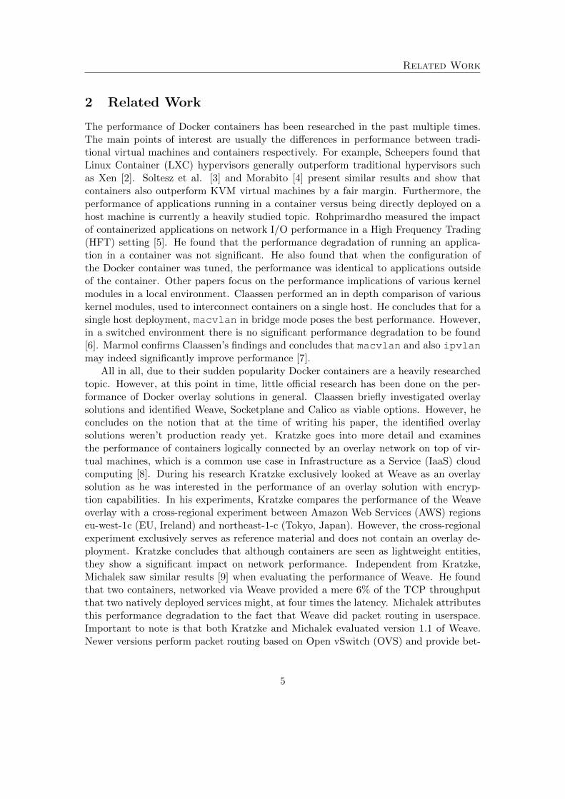
The developers of Weave and Calico go into more depth and present more detailedresults. Wragg [11] evaluated the performance of an older version (1.1) of Weave -whichhas also been evaluated by Kratzke and Michalek- and the newer version (1.2) whichincorporates OVS. Measurements were performed between two Amazon EC2 c3.8xlargeinstances with enhanced networking enabled. During the experiment, the virtual ma-chines were connected via a 10 Gbps link. Figure 1 presents the results of the comparisonbetween both Weave versions and native host performance respectively. Measurementswere performed with iperf3. Whilst using the default MTU of 1410 bytes, the per-formance deterioration of the overall TCP throughput is significant. Wragg attributesthese results to a potential bottleneck inside the kernel’s network stack. When switchingto an MTU size of approximately 9000 bytes (including the VXLAN header) the overallperformance is much closer to the performance of the underlying host. He concludesthat there is some overhead due to the VXLAN encapsulation which Weave uses, butthe results are close to those of host networking. Newer versions of Weave only see a

6

Related Work

slight decrease in performance and heavily outperform previous versions. Although thisperformance analysis is executed in a cloud environment, only a single Amazon EC2availability zone is used. As such, the experiments do not take geographical dispersioninto consideration.

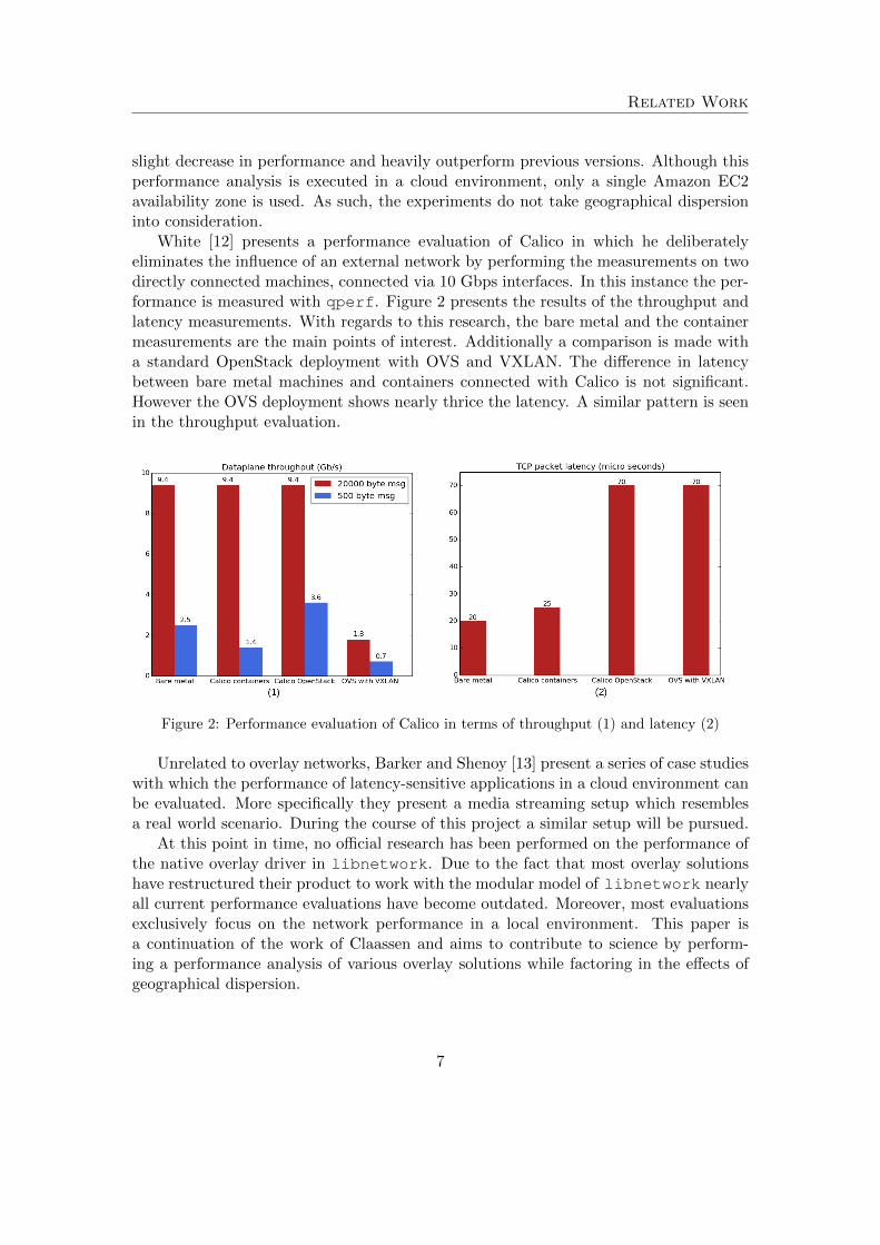
White [12] presents a performance evaluation of Calico in which he deliberatelyeliminates the influence of an external network by performing the measurements on twodirectly connected machines, connected via 10 Gbps interfaces. In this instance the per-formance is measured with qperf. Figure 2 presents the results of the throughput andlatency measurements. With regards to this research, the bare metal and the containermeasurements are the main points of interest. Additionally a comparison is made witha standard OpenStack deployment with OVS and VXLAN. The difference in latencybetween bare metal machines and containers connected with Calico is not significant.However the OVS deployment shows nearly thrice the latency. A similar pattern is seenin the throughput evaluation.

Figure 2: Performance evaluation of Calico in terms of throughput (1) and latency (2)

Unrelated to overlay networks, Barker and Shenoy [13] present a series of case studieswith which the performance of latency-sensitive applications in a cloud environment canbe evaluated. More specifically they present a media streaming setup which resemblesa real world scenario. During the course of this project a similar setup will be pursued.

At this point in time, no official research has been performed on the performance ofthe native overlay driver in libnetwork. Due to the fact that most overlay solutionshave restructured their product to work with the modular model of libnetwork nearlyall current performance evaluations have become outdated. Moreover, most evaluationsexclusively focus on the network performance in a local environment. This paper isa continuation of the work of Claassen and aims to contribute to science by perform-ing a performance analysis of various overlay solutions while factoring in the effects ofgeographical dispersion.

7

Background information

3 Background information

This section presents a brief overview of the inner workings of Docker and exploresthe technical details of the selected overlay solutions. Moreover, the GEANT TestbedsService environment is introduced.

3.1 Docker containers & networking

Docker is an open platform which aims to make building, shipping (portability), andrunning distributed applications easier [14]. In order to do so the applications are pack-aged in a ’container’. A Docker container functions as an execution environment andincludes all of the dependencies and libraries required for the application to run. Eachcontainer follows a layered model in which layers are added on top of a base imageas changes are made to the container. Figure 3 illustrates an example of this layeredstructure. On top of the read-only layers a thin read-write layer is shown. Any timea change is made to the running container, the changes are written to this read-writelayer. After all changes have been made, the layer can be committed, which creates anew Docker image. At that point, new containers can be deployed from the same image.Each container would have the same configuration and state as the container which wasused to create the image. Committing layers to an image follows a similar principle asmany version control systems employ.

Figure 3: Layered model employed by Docker containers [14]

As with traditional virtualization techniques, containers allow for running multipleisolated user space instances on a single host. However, unlike traditional VMs, theydon’t require a hypervisor layer to be active on the host machine and instead directlyshare the kernel with the host machine. [15]. Furthermore, containers exclusively containthe necessary files to run. This inherently means that containers are lightweight and canstart almost instantly. Because containers are so quick to deploy, and because they aredeployed in a ’standardized’ container format, they lend themselves to building extensive

8


microservices consisting of a multitude of independent building blocks.Figure 4 illustrates a generic workflow for deploying an application in a container.

In the figure, the Docker host is responsible for hosting the containers and maintainingthe images. By using the Docker client, the Docker daemon can be instructed to pullan image from the Docker registry. This registry is a centralized repository hosted byDocker, containing a large collection of official Docker images. This application canbe a pre-packaged application image, which in turn can directly be deployed in a newcontainer.

Figure 4: Workflow for deploying applications to Docker containers [16]

The image illustrates how a Redis application is deployed in a single Ubuntu con-tainer. Docker was originally developed to improve the application development process.Docker allowed developers to build an entire multi-tier application on a single Linuxworkstation without the complexity or overhead of multiple operating system images[17]. Because all containers were initially hosted on a single machine, Docker used arather simple networking model. By default, Docker used private networking to connectcontainers via a special virtual bridge, docker0. This bridge was allocated a subnetfrom a private IP range. In turn, every deployed container was given a virtual Ethernetinterface (usually abbreviated to ’veth’ interface) which was attached to the docker0bridge. From inside of the container, the veth interface appeared as a regular eth0interface by using Linux namespaces. Each of the veth interfaces was addressed by thedocker0 bridge in the same private subnet. As a result, the containers were able tocommunicate with each other when they were located on the same physical machineand shared the same bridge interface. Prior tot Docker version 1.9, communicating withcontainers on other hosts was difficult. In order for the containers to communicate witheach other they had to be allocated a static port on the hosting machine’s IP address.This port number was then forwarded to other containers. Inherently this meant thathosting a cluster of web servers on a single node was difficult, as ports were staticallymapped to specific containers. Connecting containers required a lot of coordination and

9


planning.By linking containers with static ports, the overall configuration used to be relatively

static. Moving containers between hosts required reconfiguration and portability waslimited. Third party overlay projects were aiming to alleviate system administratorsfrom static network configurations by connecting the containers via an an allocated IPaddress in an overlay network. Overlay networks allow for dynamically creating logicallinks between endpoints which have no coupling to the hardware infrastructure of theunderlay network, effectively abstracting out the physical network. This meant that allcontainers in the overlay network could communicate with each other, regardless of theirhost placement or the IP address of the host machine. As such, containers do not have tobe statically linked anymore based on a port number. However, early overlay solutionshad to wrap around the Docker API as multi-host networking was not supported out ofthe box.

3.2 Libnetwork

The Docker team recognized the problem of connecting containers and as of version1.9, libnetwork is included in the main release of the project. The idea behindlibnetwork is to replace the networking subsystem that was in place in previousversions of the Docker Engine with a model that allows local and remote drivers toprovide networking to containers. This means that Docker’s full networking code hasnow been included in a separate library called “libnetwork”. Docker achieved theirmodular ideal by implementing the Container Network Model (CNM). The premise ofthe CNM is that containers can be joined to networks in a multitude of ways and basedon their configuration, all containers on a given network can communicate with eachother [18]. Previously, due to the static port bindings this proved to be difficult. Withthe introduction of CNM, Docker aims to address containers more like standalone hostswhen they are deployed in overlay mode.

The innovation of the network stack was kickstarted when Docker acquired the Sock-etPlane team in March 2015 [19]. SocketPlane was one of the many available Software-Defined Networking solutions for containers on the market. Instead of connecting toa virtual bridge, each container would connect to an Open vSwitch (OVS) port. Eachcontainer host would have an OVS instance running which allowed them to form a vir-tual overlay network that would carry traffic destined for any container connected to thenetwork via VXLAN. This allows containers to seamlessly communicate with each otherwherever they are and thus enabling true distributed applications [16].

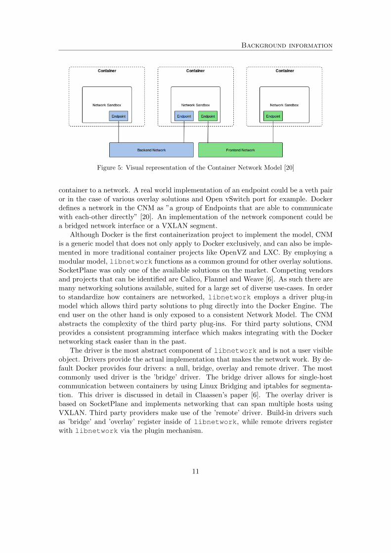
The CNM relies on three main components: the sandbox, endpoints and networks.Figure 5 presents a visual representation of the three components placed in the model. Inessence, the model is relatively simple. A (network) sandbox contains the configurationof a container’s network stack. This includes management of the container’s interfaces,routing table and DNS settings [20]. As would be the case with a standard virtualmachine, a sandbox can have multiple endpoints attached to a multitude of differentnetworks. This is also illustrated in figure 5. The middle container has two endpointsconnected to two different networks. In turn, an endpoint connects a sandbox and thus a

10


Figure 5: Visual representation of the Container Network Model [20]

container to a network. A real world implementation of an endpoint could be a veth pairor in the case of various overlay solutions and Open vSwitch port for example. Dockerdefines a network in the CNM as ”a group of Endpoints that are able to communicatewith each-other directly” [20]. An implementation of the network component could bea bridged network interface or a VXLAN segment.

Although Docker is the first containerization project to implement the model, CNMis a generic model that does not only apply to Docker exclusively, and can also be imple-mented in more traditional container projects like OpenVZ and LXC. By employing amodular model, libnetwork functions as a common ground for other overlay solutions.SocketPlane was only one of the available solutions on the market. Competing vendorsand projects that can be identified are Calico, Flannel and Weave [6]. As such there aremany networking solutions available, suited for a large set of diverse use-cases. In orderto standardize how containers are networked, libnetwork employs a driver plug-inmodel which allows third party solutions to plug directly into the Docker Engine. Theend user on the other hand is only exposed to a consistent Network Model. The CNMabstracts the complexity of the third party plug-ins. For third party solutions, CNMprovides a consistent programming interface which makes integrating with the Dockernetworking stack easier than in the past.

The driver is the most abstract component of libnetwork and is not a user visibleobject. Drivers provide the actual implementation that makes the network work. By de-fault Docker provides four drivers: a null, bridge, overlay and remote driver. The mostcommonly used driver is the ’bridge’ driver. The bridge driver allows for single-hostcommunication between containers by using Linux Bridging and iptables for segmenta-tion. This driver is discussed in detail in Claassen’s paper [6]. The overlay driver isbased on SocketPlane and implements networking that can span multiple hosts usingVXLAN. Third party providers make use of the ’remote’ driver. Build-in drivers suchas ’bridge’ and ’overlay’ register inside of libnetwork, while remote drivers registerwith libnetwork via the plugin mechanism.

11


3.3 Third party overlay solutions

During the course of this project we focus on the overlay solutions Calico, Flanneland Weave. Table 1 presents a quick overview of the technical differences betweenthe selected solutions. The successive subsections will to into more detail about eachindividual product.

Native overlay Weave Net

Native integration Libnetwork plug-inVXLAN forwarding VXLAN forwardingDedicated key-value store (any) No dedicated key-value store (CRDT)

Flannel Project Calico

No integration Libnetwork PluginUDP or VXLAN forwarding BGP routingDedicated key-value store (etcd) Dedicated key-value store (any)

Table 1: Overlay solution characteristics

3.3.1 Weave

Weave provides a Docker overlay solution named ’Weave Net’. Weave overlay consistsof a multitude of Weave routers. Such a software router is placed on every machineparticipating in the overlay. In practice, this means a Weave container is launchedwithin Docker. In addition to this container, a bridge interface is created on the hostitself. In turn, containers within the overlay (including the Weave router) connect tothis bridge using their veth interface which is supplied an IP address and subnet maskby Weave’s IP address allocator [21]. As discussed in Section 2, Weave made use ofpcap to route packets in previous versions of the project. However, as all packetshad to be moved to userspace, this resulted in a significant performance penalty. Inaddressing this issue, Weave has added ’Weave Fast Datapath’ in Weave version 1.2,which utilizes Open vSwitch [11]. This allows Weave Net to do in-kernel routing whichallows for significantly faster routing of packets between containers. Weave Router peerscommunicate their knowledge of the topology (and changes to it) to other routers, sothat all peers learn about the entire topology.

To application containers, the network established by Weave looks like a giant Ether-net switch to which all the containers are connected. In version 1.2, Weave was developedas a plug-in to libnetwork. As such, the Weave Net plugin actually provides two net-work drivers to Docker - one named weavemesh that can operate without a cluster store,and one named weave that can only work with one. By default weavemesh is utilized.As with all other overlays, Weave works alongside Docker’s existing bridge networkingcapabilities which means that single-host communication is still possible without usingWeave. In version 1.2, Weave still allows for pcap based routing when it is needed

12


in specific scenarios. By default, Weave chooses their newly introduced Fast Datapathmethod (fastdp). However, when packets have to traverse untrusted networks andrequire encryption, the slower ’sleeve’ mode is used. At this point in time Weave cannot provide encryption when using fastdp [22].

3.3.2 Flannel

Flannel is another third party solution aimed towards building overlays between Dockerhosts. The solution is part of CoreOS’ product portfolio. Whereas Weave and Calicodeploy separate container instances to manage the network, Flannel creates an agent,flanneld, on each container host which controls the overlay. All services are kept in syncvia a key-value store.

The containers and their physical hosts are stored in the etcd datastore which isalso created by CoreOS itself. Containers are assigned IP addresses from a pre-definedsubnet, which is stored in the key-value store. Other than the alternative overlays,Flannel currently does not offer integration with the libnetwork plugin. However,representatives have noted it may very well be included later [23]. By default Flannel usesUDP tunneling to connect containers. In newer versions however VXLAN forwardingwith Open vSwitch has been introduced to increase the performance of the overlaysolution [24].

As Flannel was built for Kubernetes, the solution offers tight integration with theopen source container cluster manager by Google. Kubernetes is aimed at large scaleenvironments with a multitude of containers [10].

3.3.3 Calico

Project Calico is technically not an overlay network but a pure layer 3 approach tovirtual networking. Although we primarily evaluate overlay solutions, it is still worthmentioning because Calcio strives for the same goals as overlay solutions. The ideabehind Calico is that data streams should not be encapsulated, but routed instead.This is achieved by deploying a BIRD Internet Routing Daemon on each container host.Calico uses the Border Gateway Protocol (BGP) as its control plane to advertise routesto individual containers across the physical network fabric [25].

As with Flannel and Weave, every container is assigned its own IP address froma pre-defined pool. As Calico does not connect containers via tunneling techniques,segmentation between containers is achieved by modifying the iptables configurationof the host machine. Effectively, Calico functions as a firewall between network segments.

All traffic between containers is routed at layer 3 via the Linux kernel’s native IPforwarding engine in each host. This means that no overhead is imposed when containerstry to communicate. No additional encapsulation headers are added. Like Weave, Calicofunctions as a libnetwork plug-in. The Calico network is controlled by a series ofDocker containers, managed by the calicoctl tool which exchange state informationvia the BGP routing instances. State exchange of the network is achieved with BGProute reflectors

13


3.4 Key value stores

One dependency almost all overlay solutions share is the utilization of a Key-Value(KV) stores. This NoSQL datastore is used to create a key-value database to whichthe overlays technologies write their data. While the exact way the datastore is useddiffers slightly per overlay technology, generally the values stored are related to globalIP address allocation and node discovery. In some cases additional information such ascontainer names are also stored. Weave uses it’s own proprietary storage system basedon the ’Conflict-free Replicated Data Type’ (CRDT) principle, as they believe this isbest for the availability of the overlay [26]. The other technologies support a varietyof KV-stores which are ’Consensus-Based’ (CB). One example of an open-source CBdatastore is etcd, which is the only datastore supported by all overlay technologies wewill be using (Weave excluded). If any of the datastore-systems were to malfunction,the following effects would occur:

• Inability to create new overlay networks;

• Inability to allocate global IP addresses;

• Inability to add a container to the overlay.

For the purposes of measuring the overlay performance, these implications are un-related and not an issue. This is due to the fact that we are working with a fixedenvironment and are testing performance rather than availability. Once the overlaysand containers required for testing have been created and added to the KV store, thedatastore will be idle. This means that the datastores used and their respective config-urations are of no consequence to this project.

3.5 GEANT Testbed Services

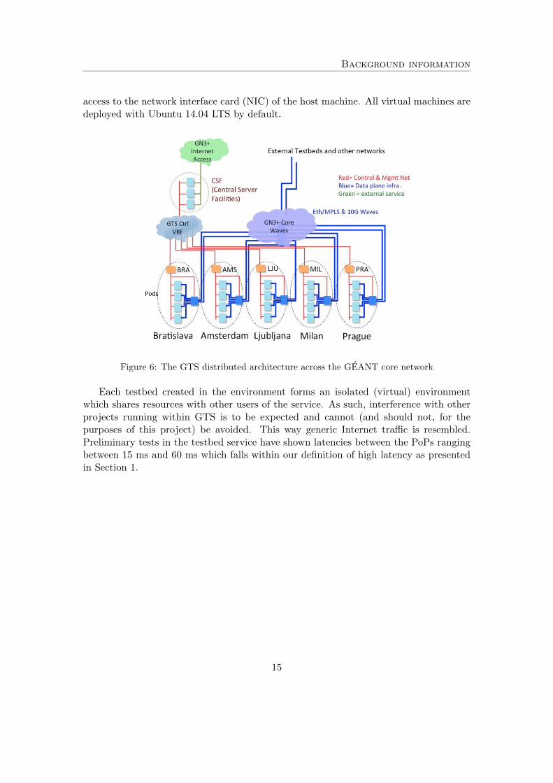
In order to do performance measurements in a realistic setting, which resembles a net-work distributed over the internet, the GEANT Testbeds Service (GTS) will be uti-lized. This service offers the ability to create experimental networks at scale, geograph-ically dispersed over five European cities. Figure 6 presents a high-level overview of theGTS environment. GEANT is a European research network which focuses on servicesaimed at research and education. GEANT has Points of Presence (PoPs) in Amsterdam,Bratislava, Ljubljana, Milan and Prague. The sites are connected via dedicated point-to-point circuits 10 Gbps optical waves in an Multi Protocol Label Switching (MPLS)cloud.

The GTS physical infrastructure is assembled into a set of equipment pods whichcontain the hardware components that make up the virtual machines, virtual circuits andother resources. Figure 6 presents a high level overview of the GTS infrastructure. Alllocations provide equal capabilities for provisioning (virtual) machines and provide equalconnectivity. The virtual machines in GTS are deployed in Kernel-based Virtual Machine(KVM) by OpenStack. Each VM uses pci passthrough, giving it full and direct

14


access to the network interface card (NIC) of the host machine. All virtual machines aredeployed with Ubuntu 14.04 LTS by default.

Figure 6: The GTS distributed architecture across the GEANT core network

Each testbed created in the environment forms an isolated (virtual) environmentwhich shares resources with other users of the service. As such, interference with otherprojects running within GTS is to be expected and cannot (and should not, for thepurposes of this project) be avoided. This way generic Internet traffic is resembled.Preliminary tests in the testbed service have shown latencies between the PoPs rangingbetween 15 ms and 60 ms which falls within our definition of high latency as presentedin Section 1.

15

Methodology

4 Methodology

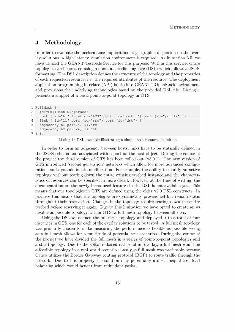
In order to evaluate the performance implications of geographic dispersion on the over-lay solutions, a high latency simulation environment is required. As in section 3.5, wehave utilized the GEANT Testbeds Service for this purpose. Within this service, entiretopologies can be created using a domain-specific language (DSL) which follows a JSONformatting. The DSL description defines the structure of the topology and the propertiesof each requested resource, i.e. the required attributes of the resource. The deploymentapplication programming interface (API) hooks into GEANT’s OpenStack environmentand provisions the underlying technologies based on the provided DSL file. Listing 1presents a snippet of a basic point-to-point topology in GTS.

1 FullMesh {2 id="FullMesh_Dispersed"3 host { id="h1" location="AMS" port {id="port11"} port {id="port12"} }4 link { id="l1" port {id="src"} port {id="dst"} }5 adjacency h1.port14, l1.src6 adjacency h2.port24, l1.dst7 } {...}

Listing 1: DSL example illustrating a simple host resource definition

In order to form an adjacency between hosts, links have to be statically defined inthe JSON schema and associated with a port on the host object. During the course ofthe project the third version of GTS has been rolled out (v3.0.1). The new version ofGTS introduced ’second generation’ networks which allow for more advanced configu-rations and dynamic in-site modification. For example, the ability to modify an activetopology without tearing down the entire existing testbed instance and the character-istics of resources can be specified in more detail. However, at the time of writing, thedocumentation on the newly introduced features in the DSL is not available yet. Thismeans that our topologies in GTS are defined using the older v2.0 DSL constructs. Inpractice this means that the topologies are dynamically provisioned but remain staticthroughout their reservation. Changes in the topology require tearing down the entiretestbed before reserving it again. Due to this limitation we have opted to create an asflexible as possible topology within GTS: a full mesh topology between all sites.

Using the DSL we defined the full mesh topology and deployed it to a total of fourinstances in GTS, one for each of the overlay solutions to be tested. A full mesh topologywas primarily chosen to make measuring the performance as flexible as possible seeingas a full mesh allows for a multitude of potential test scenarios. During the course ofthe project we have divided the full mesh in a series of point-to-point topologies anda star topology. Due to the software-based nature of an overlay, a full mesh would bea feasible topology in a real world scenario. Lastly, a full mesh was preferable becauseCalico utilizes the Border Gateway routing protocol (BGP) to route traffic through thenetwork. Due to this property the solution may potentially utilize unequal cost loadbalancing which would benefit from redundant paths.

16

Methodology

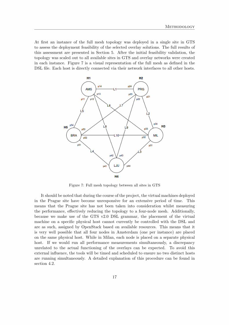
At first an instance of the full mesh topology was deployed in a single site in GTSto assess the deployment feasibility of the selected overlay solutions. The full results ofthis assessment are presented in Section 5. After the initial feasibility validation, thetopology was scaled out to all available sites in GTS and overlay networks were createdin each instance. Figure 7 is a visual representation of the full mesh as defined in theDSL file. Each host is directly connected via their network interfaces to all other hosts.

Figure 7: Full mesh topology between all sites in GTS

It should be noted that during the course of the project, the virtual machines deployedin the Prague site have become unresponsive for an extensive period of time. Thismeans that the Prague site has not been taken into consideration whilst measuringthe performance, effectively reducing the topology to a four-node mesh. Additionally,because we make use of the GTS v2.0 DSL grammar, the placement of the virtualmachine on a specific physical host cannot currently be controlled with the DSL andare as such, assigned by OpenStack based on available resources. This means that itis very well possible that all four nodes in Amsterdam (one per instance) are placedon the same physical host. While in Milan, each node is placed on a separate physicalhost. If we would run all performance measurements simultaneously, a discrepancyunrelated to the actual functioning of the overlays can be expected. To avoid thisexternal influence, the tools will be timed and scheduled to ensure no two distinct hostsare running simultaneously. A detailed explanation of this procedure can be found insection 4.2.

17

Methodology

Additionally, due to the way the virtual machines are provisioned in GTS, it isinfeasible to create a fully functional meshed topology as depicted in figure 7 with Calico.The BIRD routing daemon, which lies at the core of Calico, refuses to import a route fromthe kernel if the next-hop is not in a directly connected network. This essentially meansthat only physically connected networks can be included in the routing table as a correctBGP route, effectively limiting the topology to a point-to-point link. A workaround inorder to include the links that are not directly connected to the routing table would beto issue a route to the link and specify the route as ’onlink’. By issuing this nexthop flag (NHFLAG) with the ip command, the networking stack will pretend that thenext-hop is directly attached to the given link, even if it does not match any interfaceprefix. The NHFLAG parameter essentially instructs the kernel to treat the route as aconnected network. However, specifying this flag in the GTS returns that the NHFLAGis an invalid argument for the specified virtual interface. Moreover, whilst attemptingto create a point-to-multipoint topology, forming adjacencies between the shared nodefailed. This means that Calico’s overlay solution is limited to point-to-point topologiesbetween sites in GTS specifically. Because Calico is not suited for all desired test casesin GTS, we have have opted to drop this solution from the performance measurements.

4.1 Deployment considerations

Disregarding the local site topology, each of the deployed instances houses one of theselected overlay solutions. Due to the large amount of instances and nodes per instance,a bootstrap script has been created which handles basic machine configuration tasks andautomates the deployment of Docker. Furthermore, if desired, the script also performsthe installation and configuration of one of the respective third-party overlay solutions.For quick reference, all created scripts have been made available on GitHub 1.

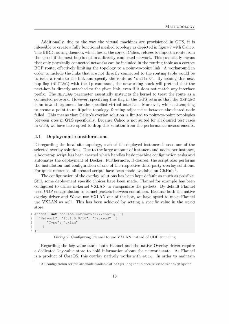
The configuration of the overlay solutions has been kept default as much as possible.Still, some deployment specific choices have been made. Flannel for example has beenconfigured to utilize in-kernel VXLAN to encapsulate the packets. By default Flannelused UDP encapsulation to tunnel packets between containers. Because both the nativeoverlay driver and Weave use VXLAN out of the box, we have opted to make Flanneluse VXLAN as well. This has been achieved by setting a specific value in the etcdstore.

1 etcdctl set /coreos.com/network//config ’{2 "Network": "10.1.0.0/16", "Backend": {3 "Type": "vxlan"4 }5 }’

Listing 2: Configuring Flannel to use VXLAN instead of UDP tunneling

Regarding the key-value store, both Flannel and the native Overlay driver requirea dedicated key-value store to hold information about the network state. As Flannelis a product of CoreOS, this overlay natively works with etcd. In order to maintain

1All configuration scripts are made available at https://github.com/siemhermans/gtsperf

18

https://github.com/siemhermans/gtsperf

Methodology

a homogeneous environment, etcd has been used for all overlays which require a key-value store. The Amsterdam site has been selected to house the etcd instance. In areal world scenario it would be desirable to deploy the key-value store as a distributedsystem in itself. However, due to the fact that process resilience is of lesser importanceduring this project we have opted to deploy a standalone instance of etcd without anyclustering. As previously discussed, the key-value store is only used by containers toregister their service and by the overlays to store the network state. As such, etcddoesn’t negatively affect performance. Because Weave utilizes an eventually consistentdistributed configuration model (CRDT), no key-value store is required for this particularoverlay.

Lastly, no specific configuration steps have been taken to integrate the overlay so-lutions with libnetwork. Current versions of Weave automatically run as a plugin,given the Docker version on the system is 1.9 or above. This means that Weave doesnot function as a wrapper to the Docker API anymore but gains more native integra-tion. As Flannel works separately from libnetwork, this overlay has been tested asa standalone. Implicitly, the native overlay driver exclusively functions as a plug-in tolibnetwork. Since the native overlay driver requires a kernel version of at least 3.16,we have upgraded all machines in GTS from their default 3.13 kernel to version 3.19with the bootstrap script.

4.2 Measurement tools

To measure the performance, iperf and netperf are used. These tools are bothindustry standard applications for benchmarking connections and are used in a multitudeof scientific papers [5], [6], [8], [13]. During our research iperf is primarily used tomeasure the UDP and TCP throughput, while netperf is primarily used to measurethe latency between sites and the effect of employing an overlay solution on the overalllatency. While iperf could technically be used to measure latency, netperf providesmore detailed statistics out of the box. Furthermore we are interested in the potentialjitter introduced by each overlay solution. Here, jitter refers to the variability in delaybetween receiving packets. Naturally, a connection with irregular intervals will have anundesirable amount of jitter which may be disruptive for latency sensitive applications.We have opted not to tune the measurement tools (e.g. the TCP window size or segmentsizes), as we are merely interested in the relative performance difference between theoverlay solutions. Whilst measuring the performance, the default parameters for bothiperf and netperf have been used. The main point of interest is running the exactsame benchmark in every situation.

Because the measurements will be performed between containers, the measurementtools have been ’dockerized’. This term refers to converting an application to run ina Docker container. This inherently means that the measurement tools are initiatedfrom within the Docker container and perform their measurements through the virtualethernet interfaces (veth) of the container and the overlay specific interfaces. Thus, bydockerizing the tools we can guarantee that we are measuring the impact of the overlaysolution and the container on performance. To dockerize the tools, a Dockerfile has

19

Methodology

been created which is displayed in full in Appendix A. The Dockerfile includes commonperformance measurement tools like iperf 2.0.5, iperf 3.0.11 and netperf 2.6.0.The Dockerfile guarantees that every deployed container is homogeneous and uses theexact same configurations and resources.

Important to note is that a patch is included in the Dockerfile for iperf 2.0.5. Thispatch, courtesy of Roderick W. Smith [27], fixes a bug that causes iperf on Linux toconsume 100% CPU at the end of a run when it’s run in daemon mode (e.g., ’iperf-sD’). After running a measurement against the iperf daemon, the process wouldremain at 100% CPU utilization. Subsequent measurements would cause the server inquestion to quickly be brought to its knees.

Figure 8: Client server model employed by the measurement tools

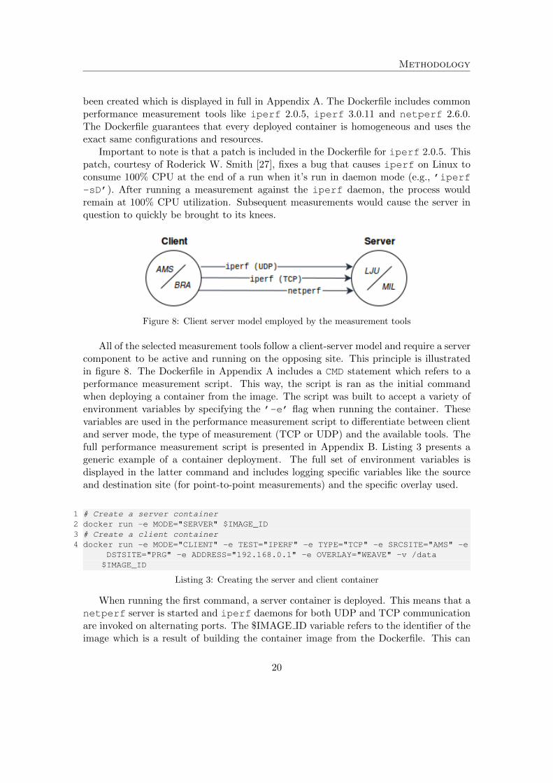
All of the selected measurement tools follow a client-server model and require a servercomponent to be active and running on the opposing site. This principle is illustratedin figure 8. The Dockerfile in Appendix A includes a CMD statement which refers to aperformance measurement script. This way, the script is ran as the initial commandwhen deploying a container from the image. The script was built to accept a variety ofenvironment variables by specifying the ’-e’ flag when running the container. Thesevariables are used in the performance measurement script to differentiate between clientand server mode, the type of measurement (TCP or UDP) and the available tools. Thefull performance measurement script is presented in Appendix B. Listing 3 presents ageneric example of a container deployment. The full set of environment variables isdisplayed in the latter command and includes logging specific variables like the sourceand destination site (for point-to-point measurements) and the specific overlay used.

1 # Create a server container2 docker run -e MODE="SERVER" $IMAGE_ID3 # Create a client container4 docker run -e MODE="CLIENT" -e TEST="IPERF" -e TYPE="TCP" -e SRCSITE="AMS" -e

DSTSITE="PRG" -e ADDRESS="192.168.0.1" -e OVERLAY="WEAVE" -v /data$IMAGE_ID

Listing 3: Creating the server and client container

When running the first command, a server container is deployed. This means that anetperf server is started and iperf daemons for both UDP and TCP communicationare invoked on alternating ports. The $IMAGE ID variable refers to the identifier of theimage which is a result of building the container image from the Dockerfile. This can

20

Methodology

be done via the ’docker build’ command. Lastly, the client command includes a’-v’ flag with an arbitrary directory. This directory, located on the underlying host, isattached as a volume to the container and is used to write logging data to.

When the client container is started, a performance measurement is ran for 115 seconds,based on the environment variables specified. When the script finishes, the containermoves to an exited state. In order to automate the measurements, cronjobs have beenused. The cronjob schedule restarts a container that has exited to perform anothermeasurement at a given interval. Generally we use a two minute interval in betweenthe cronjobs. The measurement is only ran for 115 seconds, which leaves 5 seconds ofoverhead for the application or possibly the Docker container to start and exit. It isworth noting that the daemon processes on the server never finish, and therefore willkeep running forever. This means that they are not included in any cronjobs. Becausewe are running three separate tests, three client containers are created, one for eachmeasurement tool and type. Listing 4 presents an example of a crontab and shows mea-surements for the link between the virtual machines in Bratislava and Ljubljana and thelink between the containers in each site respectively.

1 # m h dom mon dow user command2 0 * * * * root bash /root/netperf.sh 192.168.4.4 VM AMS LJU3 2 * * * * root docker start PERF_CLT_AMStoLJU4 4 * * * * root bash /root/iperf_TCP.sh 192.168.4.4 VM AMS LJU5 6 * * * * root docker start PERF_CLT_AMStoLJU_TCP6 8 * * * * root bash /root/iperf_UDP.sh 192.168.4.4 VM AMS LJU7 10 * * * * root docker start PERF_CLT_AMStoLJU_UDP

Listing 4: Crontab example for the point-to-point link between AMS and LJU

During the course of the project, Ubuntu was used as the distribution of choicewithin the virtual GTS environment as well as for the base image of the containersbecause it is a commonly available distribution with practically all cloud providers ofIaaS environments. Furthermore, Ubuntu forms a common ground for all the testedoverlay solutions with sufficient amounts of documentation available.

4.3 Experiment design

As previously discussed, the full mesh topology has been divided into multiple smallertopologies to evaluate the performance of the overlay solutions. A point-to-point topol-ogy and a star topology have been selected.

4.3.1 Baseline

In order to gain insight into the 24-hour utilization of the GTS environment, We need tostart with an initial baseline of the topology. The need for this baseline is strengthenedgiven the fact we can’t enforce the host placement of a specific virtual machine in GTS.So ideally, we would want to verify if node placement within a site is of any consequence

21

Methodology

to the performance during any point of the day. To do so, the VMs in the sites Am-sterdam and Ljubljana have been tested in parallel with Bratislava and Milan for allinstances within GTS. Only these two links have been selected for this baselining, as toincrease the amount of measurements that can be taken within a short time span. Thelinks have been chosen randomly as sites are presumed identical from the informationgathered thus far. Additionally, it has been verified some VMs reside on the differentphysical host in its respective site. Other connections of the full mesh cannot be utilizedduring the sequential tests as to avoid pollution of the results. Effectively, this functionsas a double sequential testing setup.

Each measurement taken, regardless of the tool used, will run for two minutes an hour.This is scheduled using Cronjobs. A sample of a crontab is illustrated in listing 4.

4.3.2 Point-to-Point

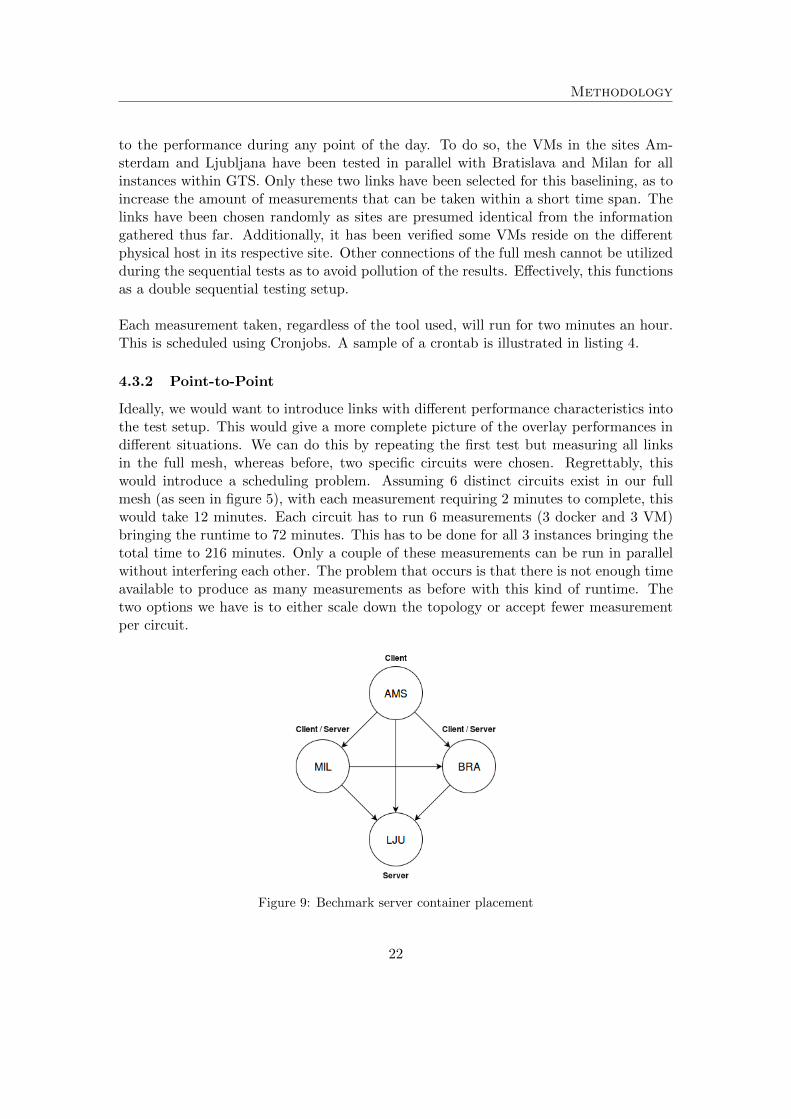
Ideally, we would want to introduce links with different performance characteristics intothe test setup. This would give a more complete picture of the overlay performances indifferent situations. We can do this by repeating the first test but measuring all linksin the full mesh, whereas before, two specific circuits were chosen. Regrettably, thiswould introduce a scheduling problem. Assuming 6 distinct circuits exist in our fullmesh (as seen in figure 5), with each measurement requiring 2 minutes to complete, thiswould take 12 minutes. Each circuit has to run 6 measurements (3 docker and 3 VM)bringing the runtime to 72 minutes. This has to be done for all 3 instances bringing thetotal time to 216 minutes. Only a couple of these measurements can be run in parallelwithout interfering each other. The problem that occurs is that there is not enough timeavailable to produce as many measurements as before with this kind of runtime. Thetwo options we have is to either scale down the topology or accept fewer measurementper circuit.

Figure 9: Bechmark server container placement

22

Methodology

The option chosen is dependent on the characteristics the previous 24-hour measure-ments have shown. If these results have shown stable performance across the board,it would be safe to conduct the four-node full mesh tests with fewer measurements. Ifthe 24-hour measurements show unsteady performance, it is best to scale the topologydown. Additionally, the 24-hour test results can be cross referenced to the new ones, tocheck if any significant deviation exists.

4.3.3 Star topology, streaming media

The previous test scenarios attempt to quantify the performance of the overlay solutionsby means of a synthetic benchmark. To provide more insight in a real world use case,we also briefly explore the effect of deploying a latency sensitive distributed applicationin each of the selected overlay solutions.

A common example of a latency sensitive system would be a streaming server, which iscapable of serving multiple clients with a video stream on demand. Streaming serversgenerally require a fast, reliable connection to prevent deterioration of the media stream,especially when the total amount of parallel streams increases. Server- and client-sidebuffering can be utilized to hide sudden variation in the network. However, high vari-ation in latency and an unpredictable throughput can still prove to be problematic forthe quality of a media stream in general.

For the purpose of this project we have opted to deploy Apple’s open-source Dar-win Streaming Server (DSS). This is the open source equivalent of Apple’s proprietaryQuickTime Streaming Server. The method utilized to perform the real world use caseroughly resembles the setup as proposed by Barker and Shenoy [13]. In their researchthe performance of several latency-sensitive applications in the Amazon EC2 cloud envi-ronment are evaluated. One of their experiments describes measuring the performanceof a media streaming server with varying amounts of background load in a point-to-pointtopology.

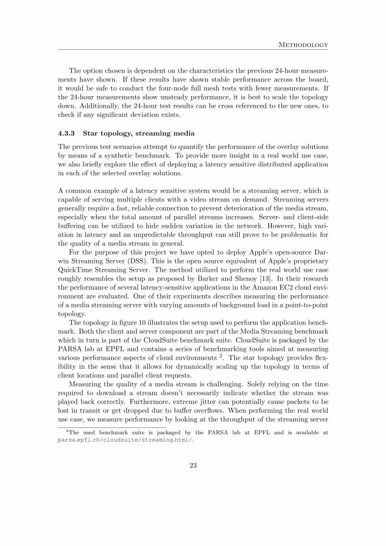
The topology in figure 10 illustrates the setup used to perform the application bench-mark. Both the client and server component are part of the Media Streaming benchmarkwhich in turn is part of the CloudSuite benchmark suite. CloudSuite is packaged by thePARSA lab at EPFL and contains a series of benchmarking tools aimed at measuringvarious performance aspects of cloud environments 2. The star topology provides flex-ibility in the sense that it allows for dynamically scaling up the topology in terms ofclient locations and parallel client requests.

Measuring the quality of a media stream is challenging. Solely relying on the timerequired to download a stream doesn’t necessarily indicate whether the stream wasplayed back correctly. Furthermore, extreme jitter can potentially cause packets to belost in transit or get dropped due to buffer overflows. When performing the real worlduse case, we measure performance by looking at the throughput of the streaming server

2The used benchmark suite is packaged by the PARSA lab at EPFL and is available atparsa.epfl.ch/cloudsuite/streaming.html/.

23

parsa.epfl.ch/cloudsuite/streaming.html/

Methodology

Figure 10: Streaming media server topology

with a varying amount of parallel streams. Ultimately we are interested in the potentialjitter introduced by the overlay solutions.

In our scenario, the DSS is placed in Bratislava and uses the Real-time TransportProtocol (RTP) for delivering the video stream to the clients via UDP. To simulateclients, Faban has been used. Faban is an open source performance workload creationand execution framework. The Faban component functions as a workload generator andemulates real world clients by creating Java workers which send requests via curl to thestreaming server. curl is compiled to support a Real-time Streaming Protocol (RTSP)library. The Media Streaming benchmark includes basic configuration file templateswhich have been modified to let Faban wait until all workers are fully up and runningbefore requesting a stream. This way a simultaneous stress-test is guaranteed withouta variable ramp up period.

On both the server and client side the network interfaces are rate limited by utilizingwondershaper. Wonder Shaper functions as a front-end to iproute’s tc commandand can limit a network adapter’s bandwidth. Limiting the bandwidth of the networkinterfaces allows us more granular control over the division of the link as well as makingthe resulting dataset from the measurements more manageable. Furthermore, by limitingthe speed of the interface the performance influence of the CPU is reduced to a minimum.

To visualize the effect of increasing the amount of clients, each of the sites is testedwith one, three and nine Java workers respectively. At maximum this results in a totalof 21 streams originating from the DSS to the clients divided over three links. For thepurpose of this experiment DSS serves up a synthetic dataset, comprising of exclusivelya stresstest video with a bit rate of 1 Mbps. The selected video contains a graduallyincreasing animation which is repeated a series of times during the measurement. This

24

Methodology

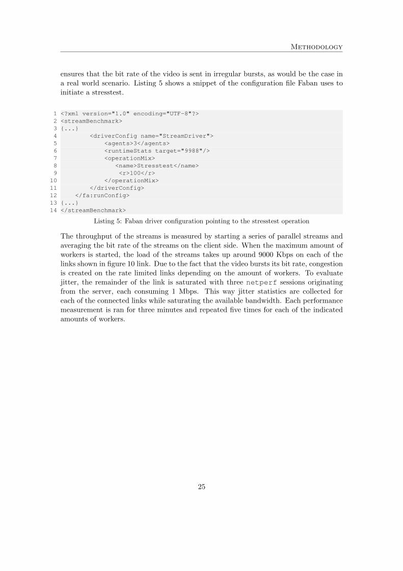
ensures that the bit rate of the video is sent in irregular bursts, as would be the case ina real world scenario. Listing 5 shows a snippet of the configuration file Faban uses toinitiate a stresstest.

1 <?xml version="1.0" encoding="UTF-8"?>2 <streamBenchmark>3 {...}4 <driverConfig name="StreamDriver">5 <agents>3</agents>6 <runtimeStats target="9988"/>7 <operationMix>8 <name>Stresstest</name>9 <r>100</r>

10 </operationMix>11 </driverConfig>12 </fa:runConfig>13 {...}14 </streamBenchmark>

Listing 5: Faban driver configuration pointing to the stresstest operation

The throughput of the streams is measured by starting a series of parallel streams andaveraging the bit rate of the streams on the client side. When the maximum amount ofworkers is started, the load of the streams takes up around 9000 Kbps on each of thelinks shown in figure 10 link. Due to the fact that the video bursts its bit rate, congestionis created on the rate limited links depending on the amount of workers. To evaluatejitter, the remainder of the link is saturated with three netperf sessions originatingfrom the server, each consuming 1 Mbps. This way jitter statistics are collected foreach of the connected links while saturating the available bandwidth. Each performancemeasurement is ran for three minutes and repeated five times for each of the indicatedamounts of workers.

25

Results

5 Results

This sections presents results of the performance measurement experiments as describedin Section 4. Because the experiments are specific to GTS, we start by commenting onthe usability of the test environment and the deployment characteristics of the overlaysolutions. Subsequently we present the results of the synthetic and the applicationbenchmark respectively.

5.1 Usability GTS

The GTS has proven to be an excellent environment for us to perform our measurementsin. The extensive documentation and rapid support enabled us to deploy topologies,specifically catered to our experiments. Still, some shortcomings in the service regardingthe usability and functionality have been identified throughout the course of the project.Shortcoming we experienced are:

• Unstable VPN initialization to the topology;

• VMs which fail to finish booting on multiple occasions;

• VMs permanently losing connectivity with the provisioning network (eth0);

• Not all DSL-features appear to be fully functional;

• Limited control over VM resources, physical placement and imaging;

• Limited control over virtual NIC of the VMs.

Mostly, these shortcomings were caused due to general availability issues. However,they did not highly impact our ability to perform the research. More significant werethe limited control options in the DSL and limited control over the networking interfaceof the virtual machine as they limited the amount of overlay solutions we were able toevaluate, as discussed in Section 4.

Whilst performing the experiments we noticed that the virtual machines deployedin GTS are relatively limited in terms of performance. By default each VM is assigneda single-core vCPU with a default speed of 2 gigahertz (GHz). Problems occurredwhen running performance measurements with iperf. The vCPU is unable to generateenough network traffic to saturate the 1 Gbps link connected to the virtual machines.Performance-wise, the only attribute which can be altered regarding the VM via the DSLis the speed of the processor with the cpuSpeed attribute. However, even when scalingup the cpuSpeed attribute to an arbitrarily high number, the speed of the processor iscapped at 2.5GHz by OpenStack. Moreover, when attempting to deploy a full mesh withan increased cpuSpeed, the instance fails to deploy. Increasing the amount of cores pervCPU is not a documented attribute and as such does not seem to be a publicly availableAPI call.

A trivial solution would be to limit the speed of the network interface card (NIC) viaethtool. However, attempting to change the speed of the interface within the virtualmachine results in an error and is not supported by the VM. Another option was to

26

Results

limit the speed of the ports attached to the containers. For this purpose the lineRateattribute can be specified in the DSL whilst defining the ports. However, the lineRateattribute is set at 1 Gbps by default and only accepts increments of 1 Gbps. Lastly, thespeed of the link between the containers can be defined within the DSL by specifying thecapacity attribute. The GTS user guide notes that the default value is 10 Mbps whichdoesn’t seem to be valid [28]. Additionally, when statically defining the capacity to be100 Mbps, the limitation does not seem to get applied. Arbitrary iperf measurementsbetween containers still indicate speeds far north of the limit. Therefore we resorted tosetting a software limit on the interface by using Wonder Shaper in the star topologyexperiment. This is also explained in Section 4.3.3

Fortunately the GTS is being frequently updated which means that some of theidentified shortcomings may be fixed in newer iterations of the service. Additionally,some of the shortcomings may be caused due to the fact that we are limited to the 2.0DSL while the service is currently running on v3.0.1. An updated user guide might solveof the issues related to deployment and control of resources.

5.2 Overlay evaluation

As previously discussed in Section 4, only Calico was infeasible to deploy due to thelimited control over the VM NIC in GTS. Flannel, Weave and the native overlay driverwere fairly straight forward to set up. During the deployment we have noticed thatWeave is by far the easiest overlay to deploy due to the fact that Weave uses CRDT toshare the network state between Weave nodes. The other overlay solutions all requirea separate key-value store for this purpose, effectively making the overall configurationmore complex. In our experiments this was achieved by by deploying a single-key valuestore in one of the sites. However, in a real world deployment where process resilience isan important factor, a clustered key-value store distributed over multiple nodes may bedesirable. This inherently means that an overlay network with these solutions requiresmanagement of another separate distributed system. Due to Weave’s ease of deploymentthe solution seems to be especially suited for Agile development and rapid prototyping.

In operation we have noticed that the control method of the overlay varies betweeneach solution. For example, Calico and Weave deploy separate containers which runthe main overlay processes for routing and state exchange. Flannel on the other handcreates a service, running on each host machine. In the case of libnetwork the overlayis controlled by the already in place Docker engine. Although we are impartial to themethod for controlling the overlay we do note that in an environment with limitedresources, the overlay process or container(s) may contend for the CPU. As discussed inSection 5.1, whilst performing our synthetic benchmark, the CPU utilization is 100%.Nevertheless, no significant performance deterioration was measured between the nativeoverlay driver and the evaluated overlay solutions. The full results of this experimentare presented in Section 5.4.

27

Results

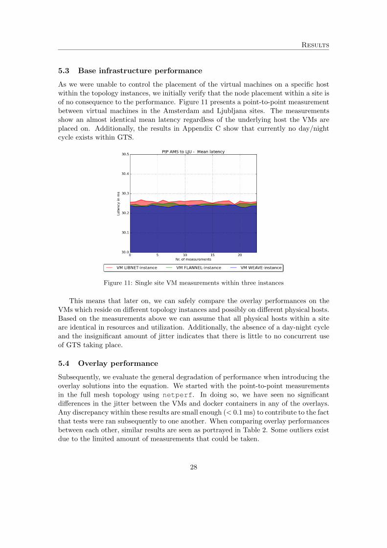
5.3 Base infrastructure performance

As we were unable to control the placement of the virtual machines on a specific hostwithin the topology instances, we initially verify that the node placement within a site isof no consequence to the performance. Figure 11 presents a point-to-point measurementbetween virtual machines in the Amsterdam and Ljubljana sites. The measurementsshow an almost identical mean latency regardless of the underlying host the VMs areplaced on. Additionally, the results in Appendix C show that currently no day/nightcycle exists within GTS.

Figure 11: Single site VM measurements within three instances

This means that later on, we can safely compare the overlay performances on theVMs which reside on different topology instances and possibly on different physical hosts.Based on the measurements above we can assume that all physical hosts within a siteare identical in resources and utilization. Additionally, the absence of a day-night cycleand the insignificant amount of jitter indicates that there is little to no concurrent useof GTS taking place.

5.4 Overlay performance

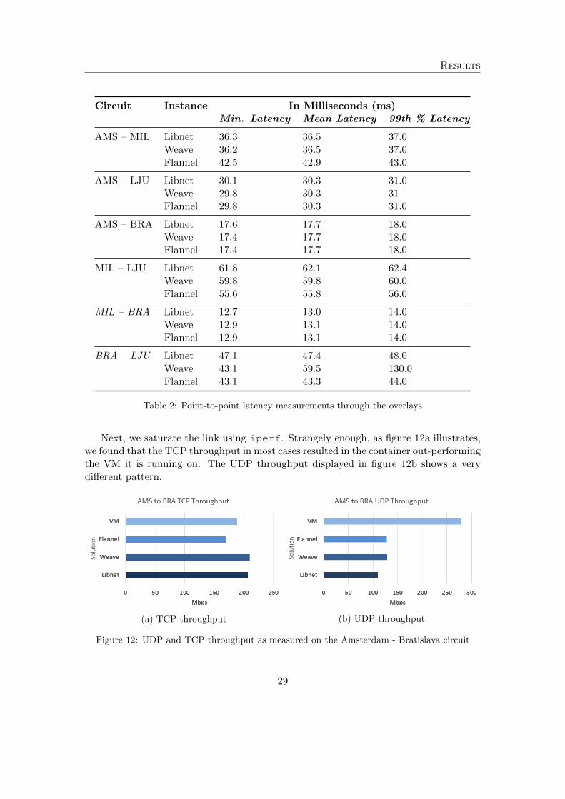
Subsequently, we evaluate the general degradation of performance when introducing theoverlay solutions into the equation. We started with the point-to-point measurementsin the full mesh topology using netperf. In doing so, we have seen no significantdifferences in the jitter between the VMs and docker containers in any of the overlays.Any discrepancy within these results are small enough (< 0.1 ms) to contribute to the factthat tests were ran subsequently to one another. When comparing overlay performancesbetween each other, similar results are seen as portrayed in Table 2. Some outliers existdue to the limited amount of measurements that could be taken.

28

Results

Circuit Instance In Milliseconds (ms)Min. Latency Mean Latency 99th % Latency

AMS – MIL Libnet 36.3 36.5 37.0Weave 36.2 36.5 37.0Flannel 42.5 42.9 43.0

AMS – LJU Libnet 30.1 30.3 31.0Weave 29.8 30.3 31Flannel 29.8 30.3 31.0

AMS – BRA Libnet 17.6 17.7 18.0Weave 17.4 17.7 18.0Flannel 17.4 17.7 18.0

MIL – LJU Libnet 61.8 62.1 62.4Weave 59.8 59.8 60.0Flannel 55.6 55.8 56.0

MIL – BRA Libnet 12.7 13.0 14.0Weave 12.9 13.1 14.0Flannel 12.9 13.1 14.0

BRA – LJU Libnet 47.1 47.4 48.0Weave 43.1 59.5 130.0Flannel 43.1 43.3 44.0

Table 2: Point-to-point latency measurements through the overlays

Next, we saturate the link using iperf. Strangely enough, as figure 12a illustrates,we found that the TCP throughput in most cases resulted in the container out-performingthe VM it is running on. The UDP throughput displayed in figure 12b shows a verydifferent pattern.

(a) TCP throughput (b) UDP throughput

Figure 12: UDP and TCP throughput as measured on the Amsterdam - Bratislava circuit

29

Results

The measured data indicates that the overlay solutions do not perform well duringUDP testing. The full results of the experiment are presented in Appendix D. Figure12 presents the results of the Amsterdam - Bratislava circuit. However, the measuredanomalies are not specific to an individual circuit as is shown in Appendix E. In somemeasurements the overlay outperforms the underlay whereas in other scenarios the op-posite is true.

Regarding the UDP throughput, Claassen examined similar behavior and hypoth-esized that the anomaly may be caused due to iperf consuming more CPU cyclesfor measuring the jitter of the UDP packets [6]. However, in his work no anomalieswere found regarding TCP throughput. This observation will be further explored in thediscussion in Section 6.

5.5 Media streaming scenario

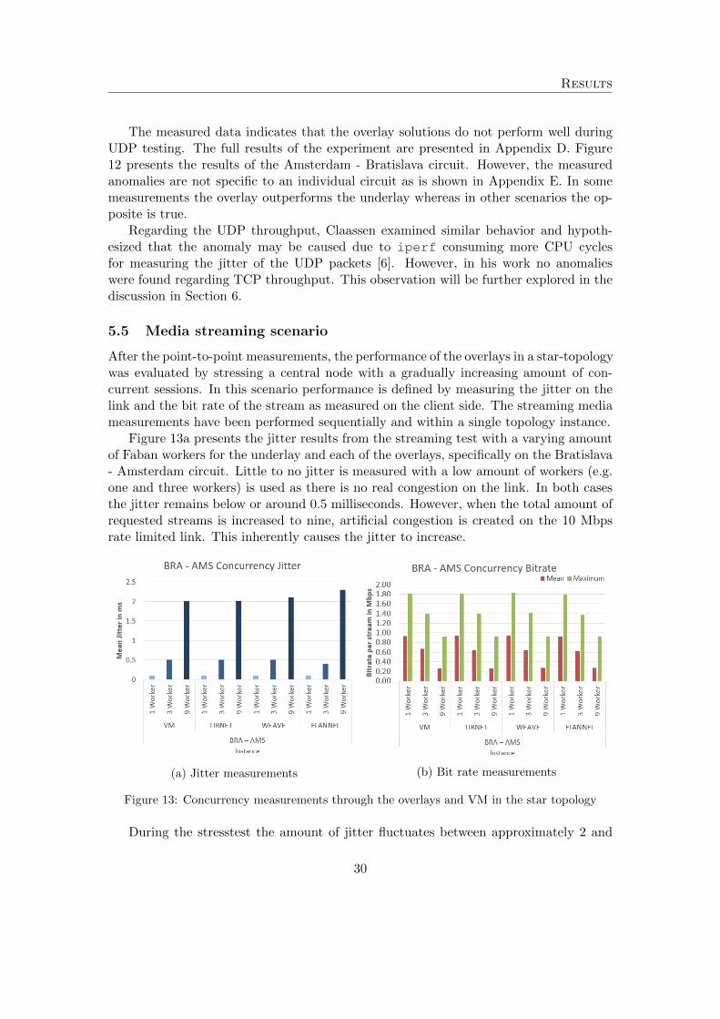
After the point-to-point measurements, the performance of the overlays in a star-topologywas evaluated by stressing a central node with a gradually increasing amount of con-current sessions. In this scenario performance is defined by measuring the jitter on thelink and the bit rate of the stream as measured on the client side. The streaming mediameasurements have been performed sequentially and within a single topology instance.

Figure 13a presents the jitter results from the streaming test with a varying amountof Faban workers for the underlay and each of the overlays, specifically on the Bratislava- Amsterdam circuit. Little to no jitter is measured with a low amount of workers (e.g.one and three workers) is used as there is no real congestion on the link. In both casesthe jitter remains below or around 0.5 milliseconds. However, when the total amount ofrequested streams is increased to nine, artificial congestion is created on the 10 Mbpsrate limited link. This inherently causes the jitter to increase.

(a) Jitter measurements (b) Bit rate measurements

Figure 13: Concurrency measurements through the overlays and VM in the star topology

During the stresstest the amount of jitter fluctuates between approximately 2 and

30

Results

2.3 milliseconds. Figure 13a shows a slight increase in jitter for Weave and Flannelrespectively, but this fluctuation is not significant and may be flattened out over thecourse of additional consecutive measurements. Furthermore, the difference in jitterbetween the virtual machines and the overlay solutions are not significant.

The measured values are below the recommendations from Cisco which state that avideo stream should have less than 30 milliseconds of one way jitter [29]. Still, Claypooland Tanner show that even low amounts of jitter can have a high impact on the perceivedquality of a video stream by end users [30]. Client- and server-side buffering can beutilized to cope with slight increases in jitter.

As expected, the results from the bit rate evaluation indicate that bit rates per streamdeteriorate when the amount of requesting clients increase. Figure 13b illustrates thatthe deterioration holds a very similar pattern between the underlay and the overlay solu-tions. There is no significant performance difference between a specific overlay solutionand the underlay. Appendix F presents the full results of the media streaming scenariofor each of the circuits as displayed in figure 10.

31

Discussion

6 Discussion

During the course of this project we measured the performance of various overlay so-lutions when implemented in a high latency environment. When starting out with theresearch, our hypothesis was that the overlay solutions would perform worse than theunderlay in any given situation. This was based on the general notion that an overlaysolution introduces an implicit performance overhead by adding another layer to thenetwork. Additionally, as most overlay solutions now resort to in-kernel traffic handling,we did not expect the decrease in performance to be very large.

The results of the point-to-point UDP and TCP throughput measurements with iperfdid not match our expectations. We saw irregular behavior whilst measuring TCPthroughput. In most situations the overlay solution outperforms the underlay but some-times the opposite is true. The measurements as presented in Appendix E indicate thatthis behavior is not specific to an individual circuit. Similarly, we expected a small de-terioration in performance whilst measuring the UDP throughput between containers inthe overlays, but not with a margin of circa 100 to 150 Mbps. Interestingly enough, ourresults indicate that the anomalies regarding UDP throughput are constant. Regardlessof the tested circuit a significant performance drop is seen.

We are not the first ones to find anomalies in UDP throughput measurements.Claassen examined similar behavior in his paper regarding Docker network performancein a local environment [6]. He hypothesized that the deterioration could be related tothe way iperf functions with regards to its utilization of CPU cycles whilst measur-ing. Regarding the disappointing UDP throughput measured with iperf, Claassen’shypothesis holds. The fact that the streaming media tests also utilize UDP and do notshow such losses does support the notion that this is indeed an iperf specific problem.Nevertheless, this does not explain why the overlay solutions outperform the underlaywhen TCP throughput is measured, which leads us to believe that this issue is specificto the GEANT Testbeds Service. Further investigation is required.

Due to the irregular results, we will presume the measurements in the point-to-pointtopology regarding UDP and TCP throughput are unreliable and as such, will not beused as a basis to form a conclusion. This decision does not impact the latency measure-ments however. These measurements consistently show that the underlay outperformsthe overlay by a very small margin (below 1 millisecond).

With regards to latency, surprisingly enough, the latency measured within GTS re-sembled that of a non-shared environment. This is likely the case due to the fact thatthe environment is not intensively being used by other researchers. Because of this, wehave been able to get unadulterated results regarding the performance of these overlays.As a consequence we have not experienced a level of congestion which would be expectedin a real world scenario. It is possible that performing the experiments in an environ-ment with a high(er) level of congestion would yield different results. This is especially

32

Discussion

true for the streaming media tests as in our current experiment we have only been ableto see the effect of artificial congestion.

During the feasibility-check of the overlay solutions, we have noticed a difference inease of setup between the different overlay technologies. Weave has proven to be themost inclusive package requiring no additional software to be installed while the otheroverlays require at least a separate key-value store. Considering there are no signifi-cant performance differences observed between the overlays -with regards to latency-,Weave could be considered the preferred solution within this specific environment. How-ever, we feel that the choice for a certain solution is very specific to the use case of thenetwork. For example, due to the fast deployment capabilities of Weave, the solutionlends itself especially well for rapid prototyping. Flannel on the other hand is built tospecifically to integrate with Google’s Kubernetes orchestration tool which allows forthe administration of very large clusters. Calico pursues a different model and is mainlyaimed at high performance data center deployments. As a closing remark we think thatthe integration a solution offers with third party tools will be a hugely deciding factorwhen selecting a solution, as all of the solutions pursue a similar goal: interconnectingcontainers dispersed over multiple hosts, regardless of their physical location.

33

Conclusion

7 Conclusion

In this paper, we have evaluated the performance of various Docker overlay solutions ina high latency environment, and more specifically, in the GEANT Testbeds Service. Weassessed the native overlay driver included in libnetwork and third party solutionsFlannel and Weave by means of a synthetic point-to-point benchmark and a streamingmedia application benchmark in a star topology. During the project, Calico was foundto be infeasible to deploy in the GTS. We saw that the remaining solutions are verysimilar on a technical level and employ similar VXLAN tunneling techniques to connectcontainers.

Our results indicate that the performance of the overlay solutions with regards to la-tency as well as jitter is very similar. The level of overhead introduced by the overlaycan be considered almost negligible (in the range of 0.1 ms). The same behavior wasfound whilst measuring the performance of the overlays in the streaming media bench-mark. All overlays exhibit similar performance, regardless of the amount of locationsin the topology or clients requesting a stream. As such, we conclude that the nativeoverlay driver performs equal to the evaluated third party solutions. Our point-to-pointmeasurements show irregular behavior with regards to UDP and TCP throughput andrequire further investigation.

Taking all of the measurements into account, we conclude that geographic dispersionhas no significant effect on either latency or jitter when evaluated in the GTS specifi-cally.

7.1 Future work

During the course of this project a GitHub repository3 has been maintained which isdesigned to make future deployments of the evaluated overlay solutions easier, particu-larly in GTS. However, although GTS is an excellent environment to test the syntheticperformance of the overlays, it would be interesting to reconduct the performance anal-ysis in a heavily shared environment (e.g. Amazon EC2 or Azure). This would requirea slight modification of the provided scripts but would illustrate the effect of real worldcongestion on performance. Additionally, the measurements should be repeated in anenvironment which is less pressed for resources, in order to eliminate the CPU as a vari-able whilst measuring. With regards to the measured results, further investigation isrequired to identify the root cause of the anomalies seen in UDP and TCP throughput.

With regards to the environment, the current measurements have been performedwith a generic Infrastructure as a Service use case in mind. This means that the Dockercontainers have been deployed within virtual machines. In the future it would be inter-esting to see how the performance of the overlay solutions compares when the containersare deployed in a special container hypervisor like LXD [31]. This would require a cloud

3All created resources are available at https://github.com/siemhermans/gtsperf

34

https://github.com/siemhermans/gtsperf

Conclusion

provider to provide (near) bare metal provision resources. At this point in time, baremetal provisioning is not supported in GTS, however, it is a confirmed road-mappedfunctionality. Therefore, the GTS may potentially be used for this purpose in the fu-ture.

35

Acknowledgements

Acknowledgements

We would like to thank Dr. Paola Grosso for guiding us throughout the course of theproject and for proofreading our initial proposal and the final report. Furthermore wewould like to thank Susanne Naegele-Jackson for providing us (preliminary) access tothe GEANT Testbeds Service. Lastly we thank Fabio Farina and Nicolai Iliuha for theirrapid response times regarding technical questions and feature requests with respect tothe GTS infrastructure.

36

REFERENCES

References

[1] Stackengine. State of containers 2015 docker adoption survey. http://www.stackengine.com/infographic-state-containers-2015-docker-adoption/, February 2015.

[2] Mathijs Jeroen Scheepers. Virtualization and containerization of application in-frastructure: A comparison. In 21st Twente Student Conference on IT, pages 1–7,2014.

[3] Stephen Soltesz, Herbert Potzl, Marc E Fiuczynski, Andy Bavier, and Larry Peter-son. Container-based operating system virtualization: a scalable, high-performancealternative to hypervisors. In ACM SIGOPS Operating Systems Review, volume 41,pages 275–287. ACM, 2007.

[4] Roberto Morabito, Jimmy Kjallman, and Miika Komu. Hypervisors vs. lightweightvirtualization: a performance comparison. In Cloud Engineering (IC2E), 2015 IEEEInternational Conference on, pages 386–393. IEEE, 2015.

[5] Rohprimardho. Measuring the Impact of Docker on Network I/O performance.http://rp.delaat.net/2014-2015/p92/report.pdf/, August 2015.

[6] Joris Claassen. Container Network Solutions. http://rp.delaat.net/2014-2015/p45/report.pdf/, July 2015.

[7] Victor Marmol, Rohit Jnagal, and Tim Hockin. Networking in Containers andContainer Clusters.

[8] Nane Kratzke. About microservices, containers and their underestimated impacton network performance. In Proceedings of CLOUD COMPUTING 2015 (6th. In-ternational Conference on Cloud Computing, GRIDS and Virtualization), pages165–169, 2015.

[9] Laurie Michalek. Weave is kinda slow. http://www.generictestdomain.net/docker/weave/networking/stupidity/2015/04/05/weave-is-kinda-slow/, April 2015.

[10] Eugene Yakubovich. Introducing flannel: An etcd backed overlay network for con-tainers. https://coreos.com/blog/introducing-rudder/, 2014.

[11] David Wragg. Weave networking performance with the new fast data path.http://blog.weave.works/2015/11/13/weave-docker-networking-performance-fast-data-path/, November 2015.

[12] Peter White. Calico dataplane performance — Project Calico. http://www.projectcalico.org/calico-dataplane-performance/, 2015.

37

http://www.stackengine.com/infographic-state-containers-2015-docker-adoption/



http://rp.delaat.net/2014-2015/p92/report.pdf/



http://www.generictestdomain.net/docker/weave/networking/stupidity/2015/04/05/weave-is-kinda-slow/



https://coreos.com/blog/introducing-rudder/

http://blog.weave.works/2015/11/13/weave-docker-networking-performance-fast-data-path/

http://blog.weave.works/2015/11/13/weave-docker-networking-performance-fast-data-path/

http://www.projectcalico.org/calico-dataplane-performance/

http://www.projectcalico.org/calico-dataplane-performance/

REFERENCES

[13] Sean Kenneth Barker and Prashant Shenoy. Empirical evaluation of latency-sensitive application performance in the cloud. In Proceedings of the first annualACM SIGMM conference on Multimedia systems, pages 35–46. ACM, 2010.

[14] Docker. What is docker? https://www.docker.com/what-docker, 2015.

[15] James Turnbull. The Docker Book. Lulu. com, 2014.

[16] Dave Tucker. Multi-host docker networking is now ready for production. https://blog.docker.com/2015/11/docker-multi-host-networking-ga/, 2015.

[17] Keith Townsend. Socketplane strives to alleviate docker networking challenges- techrepublic. http://www.techrepublic.com/article/socketplane-strives-to-alleviate-docker-networking-challenges/, 2015.

[18] Michael Bridgen. Weave as a docker network plugin. http://blog.weave.works/2015/06/22/weave-as-a-docker-network-plugin/, 2015.

[19] Brent Salisbury. Socketplane excited to be joining docker to collabo-rate with networking ecosystem. https://blog.docker.com/2015/03/socketplane-excited-to-be-joining-docker-to-collaborate-with-networking-ecosystem/, 2015.

[20] Docker. Libnetwork design document. https://github.com/docker/libnetwork/blob/master/docs/design.md, 2015.

[21] Weave Works. How weave works. http://docs.weave.works/weave/latest release/how-it-works.html, 2015.

[22] David Wragg. Weave 1.2 docker container networking is fast, 2015.

[23] Eugene Y. Coreos, flannel and docker networking. https://groups.google.com/forum/#!topic/coreos-user/Kl7ejtcRxbc, Octo-ber.

[24] CoreOS. Configuring flannel for container networking. https://coreos.com/flannel/docs/latest/flannel-config.html, 2015.

[25] Project Calico. Difficulties with traditional overlay networks. http://www.projectcalico.org/learn/, 2015.

[26] Alexis Richardson. Docker networking 1.9 and weave technical deep-dive. http://blog.weave.works/2015/11/03/docker-networking-1-9-technical-deep-dive/, 2015.

[27] Roderick W. Smith. Iperf CPU consumption at the end of a run in daemon mode.http://sourceforge.net/p/iperf/patches/28/, July 2014.

38

https://www.docker.com/what-docker

https://blog.docker.com/2015/11/docker-multi-host-networking-ga/

https://blog.docker.com/2015/11/docker-multi-host-networking-ga/

http://www.techrepublic.com/article/socketplane-strives-to-alleviate-docker-networking-challenges/

http://www.techrepublic.com/article/socketplane-strives-to-alleviate-docker-networking-challenges/

http://blog.weave.works/2015/06/22/weave-as-a-docker-network-plugin/



https://blog.docker.com/2015/03/socketplane-excited-to-be-joining-docker-to-collaborate-with-networking-ecosystem/



https://github.com/docker/libnetwork/blob/master/docs/design.md

https://github.com/docker/libnetwork/blob/master/docs/design.md

http://docs.weave.works/weave/latest_release/how-it-works.html

http://docs.weave.works/weave/latest_release/how-it-works.html

https://groups.google.com/forum/#!topic/coreos-user/Kl7ejtcRxbc

https://groups.google.com/forum/#!topic/coreos-user/Kl7ejtcRxbc

https://coreos.com/flannel/docs/latest/flannel-config.html

https://coreos.com/flannel/docs/latest/flannel-config.html

http://www.projectcalico.org/learn/

http://www.projectcalico.org/learn/

http://blog.weave.works/2015/11/03/docker-networking-1-9-technical-deep-dive/

http://blog.weave.works/2015/11/03/docker-networking-1-9-technical-deep-dive/

http://sourceforge.net/p/iperf/patches/28/

REFERENCES

[28] Susanne Naegele-Jackson, Michal Hazlinsky, Fabio Farina, and Nicolai Iliuha.GEANT Testbed Service (GTS) User and Resource Guide. 2 edition, 2015.

[29] Tim Szigeti and Christina Hattingh. Quality of service design overview ¿ qos require-ments of voip. http://www.ciscopress.com/articles/article.asp?p=357102&seqNum=2, 2004.

[30] Mark Claypool and Jonathan Tanner. The effects of jitter on the peceptual qualityof video. In Proceedings of the seventh ACM international conference on Multimedia(Part 2), pages 115–118. ACM, 1999.

[31] Ubuntu.com. LXD: the next-generation container hypervisor for Linux. http://www.ubuntu.com/cloud/lxd.

39

http://www.ciscopress.com/articles/article.asp?p=357102&seqNum=2

http://www.ciscopress.com/articles/article.asp?p=357102&seqNum=2

http://www.ubuntu.com/cloud/lxd

http://www.ubuntu.com/cloud/lxd

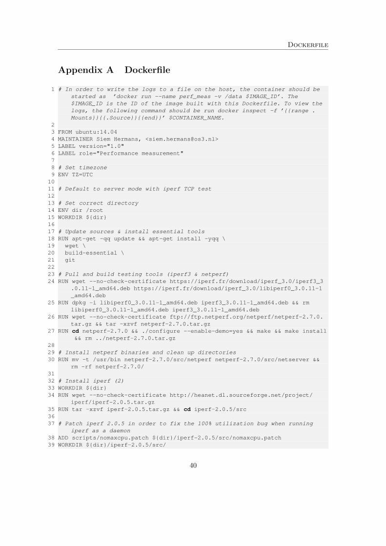
Dockerfile

Appendix A Dockerfile

1 # In order to write the logs to a file on the host, the container should bestarted as ’docker run --name perf_meas -v /data $IMAGE_ID’. The$IMAGE_ID is the ID of the image built with this Dockerfile. To view thelogs, the following command should be run docker inspect -f ’{{range .Mounts}}{{.Source}}{{end}}’ $CONTAINER_NAME.

23 FROM ubuntu:14.044 MAINTAINER Siem Hermans, <[email protected]>5 LABEL version="1.0"6 LABEL role="Performance measurement"78 # Set timezone9 ENV TZ=UTC

1011 # Default to server mode with iperf TCP test1213 # Set correct directory14 ENV dir /root15 WORKDIR ${dir}1617 # Update sources & install essential tools18 RUN apt-get -qq update && apt-get install -yqq \19 wget \20 build-essential \21 git2223 # Pull and build testing tools (iperf3 & netperf)24 RUN wget --no-check-certificate https://iperf.fr/download/iperf_3.0/iperf3_3

.0.11-1_amd64.deb https://iperf.fr/download/iperf_3.0/libiperf0_3.0.11-1_amd64.deb

25 RUN dpkg -i libiperf0_3.0.11-1_amd64.deb iperf3_3.0.11-1_amd64.deb && rmlibiperf0_3.0.11-1_amd64.deb iperf3_3.0.11-1_amd64.deb

26 RUN wget --no-check-certificate ftp://ftp.netperf.org/netperf/netperf-2.7.0.tar.gz && tar -xzvf netperf-2.7.0.tar.gz

27 RUN cd netperf-2.7.0 && ./configure --enable-demo=yes && make && make install&& rm ../netperf-2.7.0.tar.gz

2829 # Install netperf binaries and clean up directories30 RUN mv -t /usr/bin netperf-2.7.0/src/netperf netperf-2.7.0/src/netserver &&

rm -rf netperf-2.7.0/3132 # Install iperf (2)33 WORKDIR ${dir}34 RUN wget --no-check-certificate http://heanet.dl.sourceforge.net/project/

iperf/iperf-2.0.5.tar.gz35 RUN tar -xzvf iperf-2.0.5.tar.gz && cd iperf-2.0.5/src3637 # Patch iperf 2.0.5 in order to fix the 100% utilization bug when running

iperf as a daemon38 ADD scripts/nomaxcpu.patch ${dir}/iperf-2.0.5/src/nomaxcpu.patch39 WORKDIR ${dir}/iperf-2.0.5/src/

40

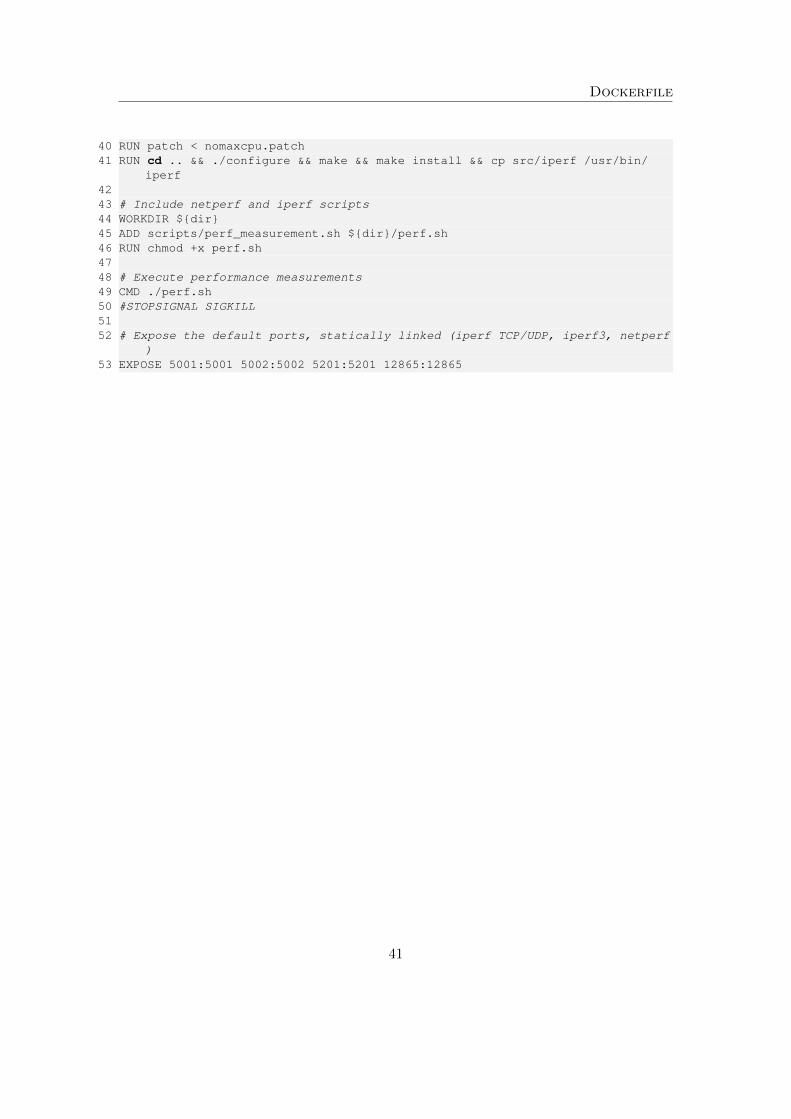
Dockerfile

40 RUN patch < nomaxcpu.patch41 RUN cd .. && ./configure && make && make install && cp src/iperf /usr/bin/

iperf4243 # Include netperf and iperf scripts44 WORKDIR ${dir}45 ADD scripts/perf_measurement.sh ${dir}/perf.sh46 RUN chmod +x perf.sh4748 # Execute performance measurements49 CMD ./perf.sh50 #STOPSIGNAL SIGKILL5152 # Expose the default ports, statically linked (iperf TCP/UDP, iperf3, netperf

)53 EXPOSE 5001:5001 5002:5002 5201:5201 12865:12865

41

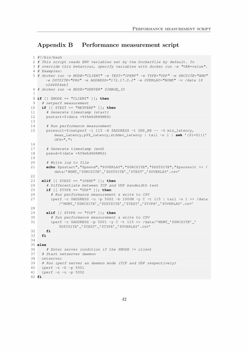
Performance measurement script

Appendix B Performance measurement script

1 #!/bin/bash2 # This script reads ENV variables set by the Dockerfile by default. To3 # override this behaviour, specify variables with docker run -e "VAR=value".4 # Examples:5 # docker run -e MODE="CLIENT" -e TEST="IPERF" -e TYPE="UDP" -e SRCSITE="AMS"

-e DSTSITE="PRG" -e ADDRESS="172.17.0.2" -e OVERLAY="NONE" -v /data 18c2d4864eb3

6 # docker run -e MODE="SERVER" $IMAGE_ID78 if [[ $MODE == "CLIENT" ]]; then9 # netperf measurement

10 if [[ $TEST == "NETPERF" ]]; then11 # Generate timestamp (start)12 psstart=$(date +%Y%m%d%H%M%S)1314 # Run performance measurement15 psresult=$(netperf -l 115 -H $ADDRESS -t UDP_RR -- -O min_latency,

mean_latency,p99_latency,stddev_latency | tail -n 1 | awk ’{$1=$1}1’OFS=",")

1617 # Generate timestamp (end)18 psend=$(date +%Y%m%d%H%M%S)1920 # Write log to file21 echo $psstart","$psend","$OVERLAY","$SRCSITE","$DSTSITE","$psresult >> /

data/’MSMT_’$SRCSITE’_’$DSTSITE’_’$TEST’_’$OVERLAY’.csv’2223 elif [[ $TEST == "IPERF" ]]; then24 # Differentiate between TCP and UDP bandwidth test25 if [[ $TYPE == "UDP" ]]; then26 # Run performance measurement & write to CSV27 iperf -c $ADDRESS -u -p 5002 -b 1000M -y C -t 115 | tail -n 1 >> /data

/’MSMT_’$SRCSITE’_’$DSTSITE’_’$TEST’_’$TYPE’_’$OVERLAY’.csv’2829 elif [[ $TYPE == "TCP" ]]; then30 # Run performance measurement & write to CSV31 iperf -c $ADDRESS -p 5001 -y C -t 115 >> /data/’MSMT_’$SRCSITE’_’

$DSTSITE’_’$TEST’_’$TYPE’_’$OVERLAY’.csv’32 fi33 fi3435 else36 # Enter server condition if the $MODE != client37 # Start netserver daemon38 netserver39 # Run iperf server as daemon mode (TCP and UDP respectively)40 iperf -s -D -p 500141 iperf -s -u -p 500242 fi

42

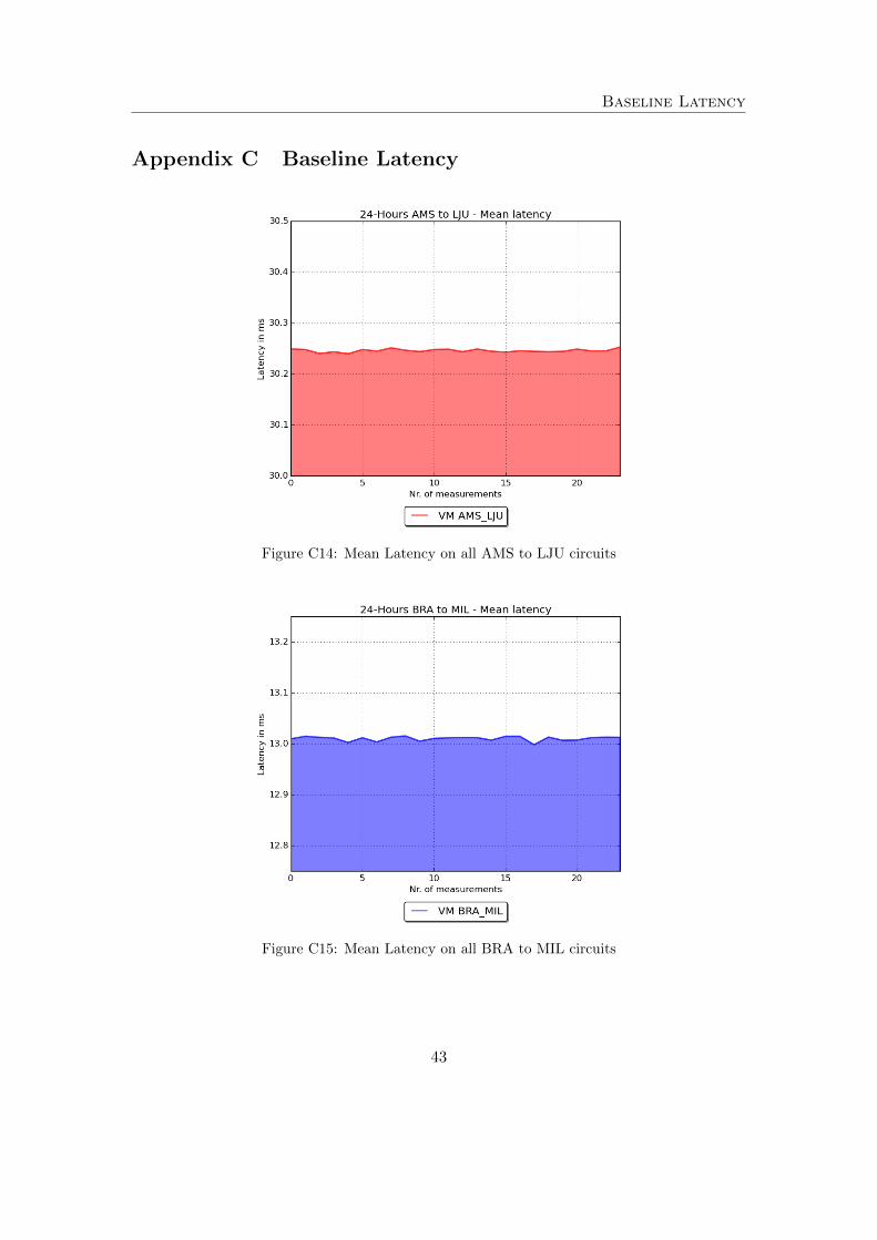
Baseline Latency

Appendix C Baseline Latency

Figure C14: Mean Latency on all AMS to LJU circuits

Figure C15: Mean Latency on all BRA to MIL circuits

43

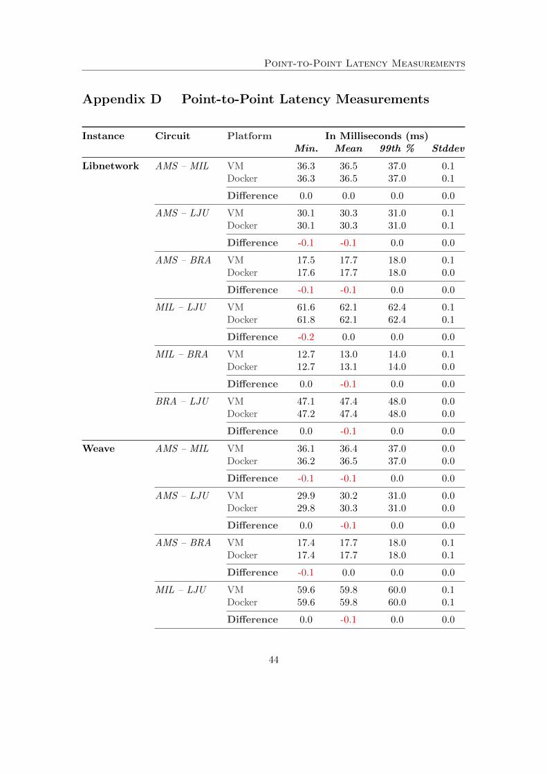
Point-to-Point Latency Measurements

Appendix D Point-to-Point Latency Measurements

Instance Circuit Platform In Milliseconds (ms)Min. Mean 99th % Stddev

Libnetwork AMS – MIL VM 36.3 36.5 37.0 0.1Docker 36.3 36.5 37.0 0.1

Difference 0.0 0.0 0.0 0.0

AMS – LJU VM 30.1 30.3 31.0 0.1Docker 30.1 30.3 31.0 0.1

Difference -0.1 -0.1 0.0 0.0

AMS – BRA VM 17.5 17.7 18.0 0.1Docker 17.6 17.7 18.0 0.0

Difference -0.1 -0.1 0.0 0.0

MIL – LJU VM 61.6 62.1 62.4 0.1Docker 61.8 62.1 62.4 0.1

Difference -0.2 0.0 0.0 0.0

MIL – BRA VM 12.7 13.0 14.0 0.1Docker 12.7 13.1 14.0 0.0

Difference 0.0 -0.1 0.0 0.0

BRA – LJU VM 47.1 47.4 48.0 0.0Docker 47.2 47.4 48.0 0.0

Difference 0.0 -0.1 0.0 0.0

Weave AMS – MIL VM 36.1 36.4 37.0 0.0Docker 36.2 36.5 37.0 0.0

Difference -0.1 -0.1 0.0 0.0

AMS – LJU VM 29.9 30.2 31.0 0.0Docker 29.8 30.3 31.0 0.0

Difference 0.0 -0.1 0.0 0.0

AMS – BRA VM 17.4 17.7 18.0 0.1Docker 17.4 17.7 18.0 0.1

Difference -0.1 0.0 0.0 0.0

MIL – LJU VM 59.6 59.8 60.0 0.1Docker 59.6 59.8 60.0 0.1

Difference 0.0 -0.1 0.0 0.0

44

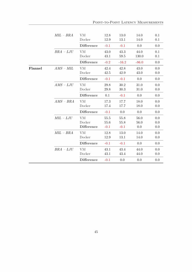
Point-to-Point Latency Measurements

MIL – BRA VM 12.8 13.0 14.0 0.1Docker 12.9 13.1 14.0 0.1

Difference -0.1 -0.1 0.0 0.0

BRA – LJU VM 43.0 43.3 44.0 0.1Docker 43.1 59.5 130.0 0.1

Difference -0.2 -16.2 -86.0 0.0

Flannel AMS – MIL VM 42.4 42.8 43.0 0.0Docker 42.5 42.9 43.0 0.0

Difference -0.1 -0.1 0.0 0.0

AMS – LJU VM 29.8 30.2 31.0 0.0Docker 29.8 30.3 31.0 0.0

Difference 0.1 -0.1 0.0 0.0

AMS – BRA VM 17.3 17.7 18.0 0.0Docker 17.4 17.7 18.0 0.0

Difference -0.1 0.0 0.0 0.0

MIL – LJU VM 55.5 55.8 56.0 0.0Docker 55.6 55.8 56.0 0.0Difference -0.1 -0.1 0.0 0.0

MIL – BRA VM 12.8 13.0 14.0 0.0Docker 12.9 13.1 14.0 0.0

Difference -0.1 -0.1 0.0 0.0

BRA – LJU VM 43.1 43.4 44.0 0.0Docker 43.1 43.4 44.0 0.0

Difference -0.1 0.0 0.0 0.0

45

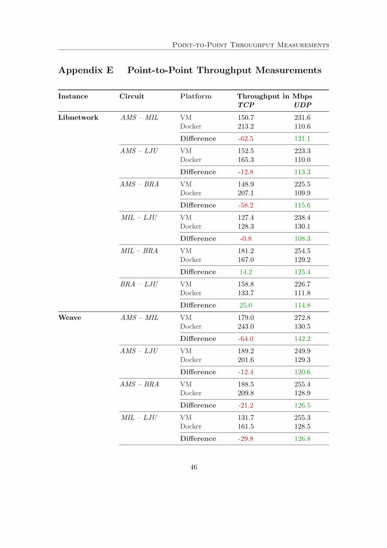
Point-to-Point Throughput Measurements

Appendix E Point-to-Point Throughput Measurements

Instance Circuit Platform Throughput in MbpsTCP UDP

Libnetwork AMS – MIL VM 150.7 231.6Docker 213.2 110.6

Difference -62.5 121.1

AMS – LJU VM 152.5 223.3Docker 165.3 110.0


AMS – BRA VM 148.9 225.5Docker 207.1 109.9


MIL – LJU VM 127.4 238.4Docker 128.3 130.1


MIL – BRA VM 181.2 254.5Docker 167.0 129.2

Difference 14.2 125.4

BRA – LJU VM 158.8 226.7Docker 133.7 111.8


Weave AMS – MIL VM 179.0 272.8Docker 243.0 130.5


AMS – LJU VM 189.2 249.9Docker 201.6 129.3


AMS – BRA VM 188.5 255.4Docker 209.8 128.9


MIL – LJU VM 131.7 255.3Docker 161.5 128.5


46

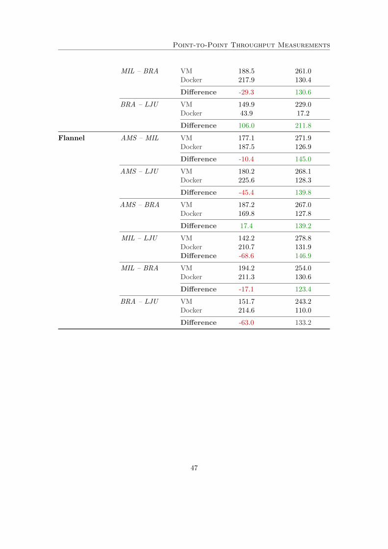
Point-to-Point Throughput Measurements

MIL – BRA VM 188.5 261.0Docker 217.9 130.4


BRA – LJU VM 149.9 229.0Docker 43.9 17.2


Flannel AMS – MIL VM 177.1 271.9Docker 187.5 126.9


AMS – LJU VM 180.2 268.1Docker 225.6 128.3


AMS – BRA VM 187.2 267.0Docker 169.8 127.8


MIL – LJU VM 142.2 278.8Docker 210.7 131.9Difference -68.6 146.9

MIL – BRA VM 194.2 254.0Docker 211.3 130.6


BRA – LJU VM 151.7 243.2Docker 214.6 110.0


47

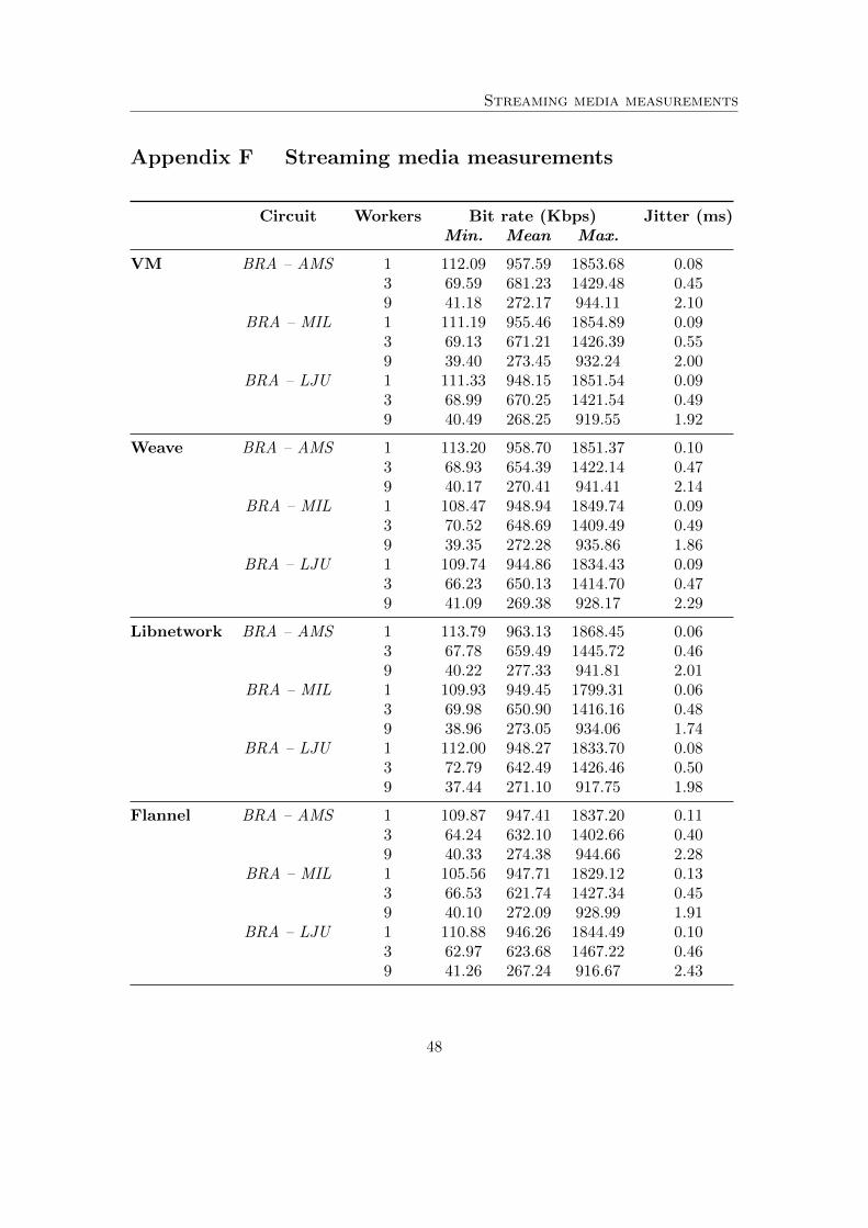
Streaming media measurements

Appendix F Streaming media measurements

Circuit Workers Bit rate (Kbps) Jitter (ms)Min. Mean Max.

VM BRA – AMS 1 112.09 957.59 1853.68 0.083 69.59 681.23 1429.48 0.459 41.18 272.17 944.11 2.10

BRA – MIL 1 111.19 955.46 1854.89 0.093 69.13 671.21 1426.39 0.559 39.40 273.45 932.24 2.00

BRA – LJU 1 111.33 948.15 1851.54 0.093 68.99 670.25 1421.54 0.499 40.49 268.25 919.55 1.92

Weave BRA – AMS 1 113.20 958.70 1851.37 0.103 68.93 654.39 1422.14 0.479 40.17 270.41 941.41 2.14

BRA – MIL 1 108.47 948.94 1849.74 0.093 70.52 648.69 1409.49 0.499 39.35 272.28 935.86 1.86

BRA – LJU 1 109.74 944.86 1834.43 0.093 66.23 650.13 1414.70 0.479 41.09 269.38 928.17 2.29

Libnetwork BRA – AMS 1 113.79 963.13 1868.45 0.063 67.78 659.49 1445.72 0.469 40.22 277.33 941.81 2.01

BRA – MIL 1 109.93 949.45 1799.31 0.063 69.98 650.90 1416.16 0.489 38.96 273.05 934.06 1.74

BRA – LJU 1 112.00 948.27 1833.70 0.083 72.79 642.49 1426.46 0.509 37.44 271.10 917.75 1.98

Flannel BRA – AMS 1 109.87 947.41 1837.20 0.113 64.24 632.10 1402.66 0.409 40.33 274.38 944.66 2.28

BRA – MIL 1 105.56 947.71 1829.12 0.133 66.53 621.74 1427.34 0.459 40.10 272.09 928.99 1.91

BRA – LJU 1 110.88 946.26 1844.49 0.103 62.97 623.68 1467.22 0.469 41.26 267.24 916.67 2.43

48

Documents

Docker Overlay Networks - OS3 · Docker Overlay Networks Performance analysis in high-latency environments MSc Research Project ... Socketplane and Calico as viable options. However,