ENB7060TELECOMMUNICATIONS B

LABORATORY SHEET 5

__________________________________________________________________________________________Name:- (Type Your Name Here)

Student ID :- (Type Your Student ID Here)

Objective

The main objectives of this experiment is to perform the following objectives using communication toolbox in matlab and Simulink :

Part I) To perform digital modulation/demodulation techniques and plot the signal constellation associated with a modulation process using communications toolbox.

Part III) To generate BER data for analyzing communication systems (modulator-chanel-demodulator) using BERTool.

Part I) To perform simulations for digital modulation/demodulation techniques sing simulink.

Learning Outcome:This lab assignment satisfies the learning outcome #2, which is, to evaluate and compare different modulation/demodulation techniquesMarking Scheme

Marks Assigned

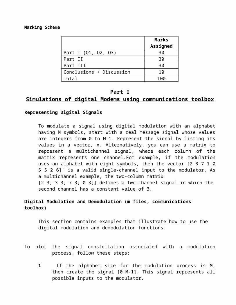
Part I (Q1, Q2, Q3) 30Part II 30Part III 30Conclusions + Discussion 10Total 100

Digital Baseband Modulation/Demodulation Techniques

Hands on Bit error calculations, Signal space analysis and Receivers design

Part I Simulations of digital Modems using communications toolbox

Representing Digital Signals

To modulate a signal using digital modulation with an alphabet having M symbols, start with a real message signal whose values are integers from 0 to M-1. Represent the signal by listing its values in a vector, x. Alternatively, you can use a matrix to represent a multichannel signal, where each column of the matrix represents one channel.For example, if the modulation uses an alphabet with eight symbols, then the vector [2 3 7 1 0 5 5 2 6]' is a valid single-channel input to the modulator. As a multichannel example, the two-column matrix[2 3; 3 3; 7 3; 0 3;] defines a two-channel signal in which the second channel has a constant value of 3.

Digital Modulation and Demodulation (m files, communications toolbox)

This section contains examples that illustrate how to use the digital modulation and demodulation functions.

To plot the signal constellation associated with a modulation process, follow these steps:

1 If the alphabet size for the modulation process is M, then create the signal [0:M-1]. This signal represents all possible inputs to the modulator.

2 Use the appropriate modulation function to modulate this signal. If desired, scale the output. The result is the set of all points of the signal constellation.

3 Apply the scatterplot function to the modulated output to create a plot.

Example (1): Computing the Symbol Error Rate

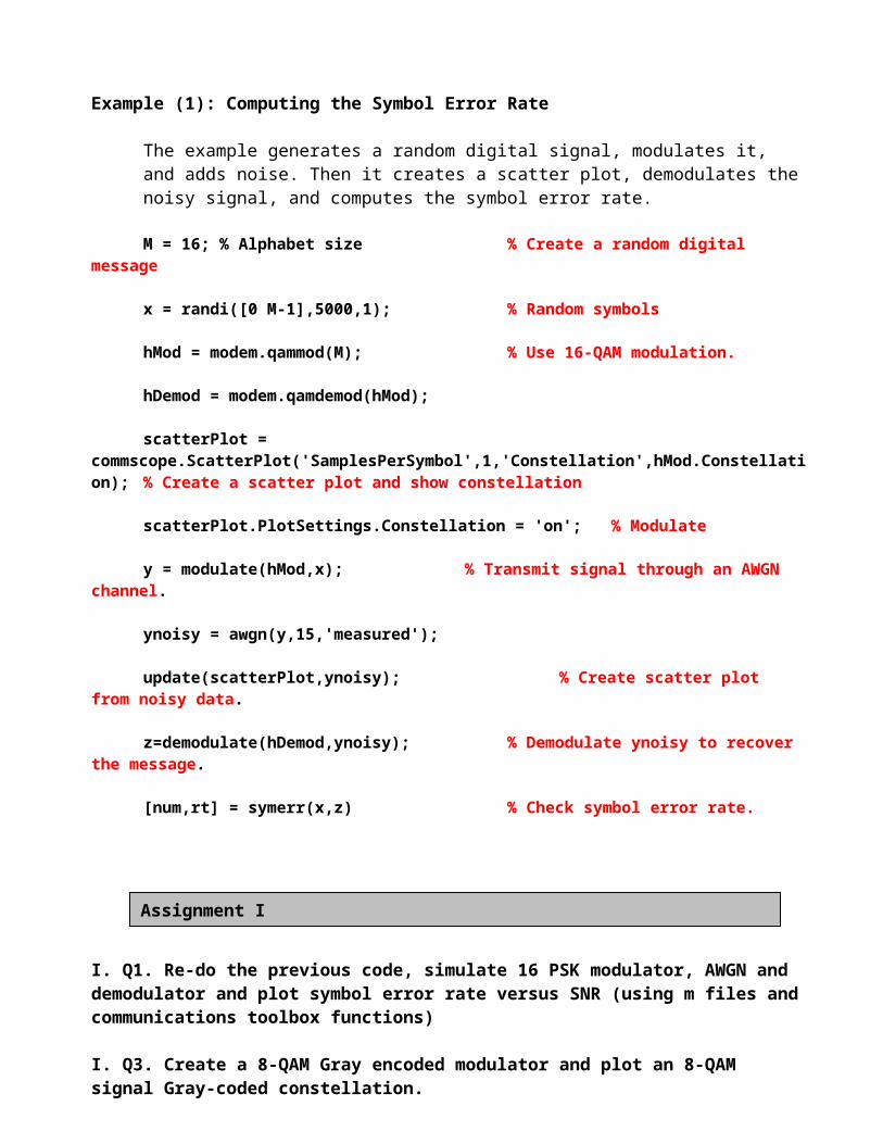
The example generates a random digital signal, modulates it, and adds noise. Then it creates a scatter plot, demodulates the noisy signal, and computes the symbol error rate.

M = 16; % Alphabet size % Create a random digital message

x = randi([0 M-1],5000,1); % Random symbols

hMod = modem.qammod(M); % Use 16-QAM modulation.

hDemod = modem.qamdemod(hMod);

scatterPlot = commscope.ScatterPlot('SamplesPerSymbol',1,'Constellation',hMod.Constellation); % Create a scatter plot and show constellation

scatterPlot.PlotSettings.Constellation = 'on'; % Modulate

y = modulate(hMod,x); % Transmit signal through an AWGN channel.

ynoisy = awgn(y,15,'measured');

update(scatterPlot,ynoisy); % Create scatter plot from noisy data.

z=demodulate(hDemod,ynoisy); % Demodulate ynoisy to recover the message.

[num,rt] = symerr(x,z) % Check symbol error rate.

I. Q1. Re-do the previous code, simulate 16 PSK modulator, AWGN and demodulator and plot symbol error rate versus SNR (using m files and communications toolbox functions)

I. Q3. Create a 8-QAM Gray encoded modulator and plot an 8-QAM signal Gray-coded constellation.

I. Q2. Create a 64-QAM modulator/demodulator and plot a QAM constellation at the receiver having 64 points at three different signal to noise ratios.

Assignment I

Part IITo generate BER data for analyzing communication systems using BERTool

BERTool is an interactive GUI for analyzing communication systems’ bit error rate (BER) performance. Using BERTool you can

• Generate BER data for a communication system using

- Closed-form expressions for theoretical BER performance of selected types of communication systems.

- Calculating BER using semi-analytical technique.

- Simulations contained in MATLAB simulation functions or Simulink models. After you create a function or model that simulates the system, BERTool iterates over your choice of Eb/N0 values and collects the results.

• Plot one or more BER data sets on a single set of axes. For example,you can graphically compare simulation data with theoretical results or simulation data from a series of similar models of a communication system.

• Fit a curve to a set of simulation data.

• Send BER data to the MATLAB workspace or to a file for any further processing you might want to perform.

There are three different methods by which BERTool can generate BER data.They are

Theoretical Semianalytic Monte Carlo

Computing Theoretical BER

You can use BERTool to generate and analyze theoretical BER data.Theoretical data is useful for comparison with your simulation results. However, closed-form BER expressions exist only for certain kinds of communication systems. To access the capabilities of BERTool related to theoretical BER data, use the following procedure:

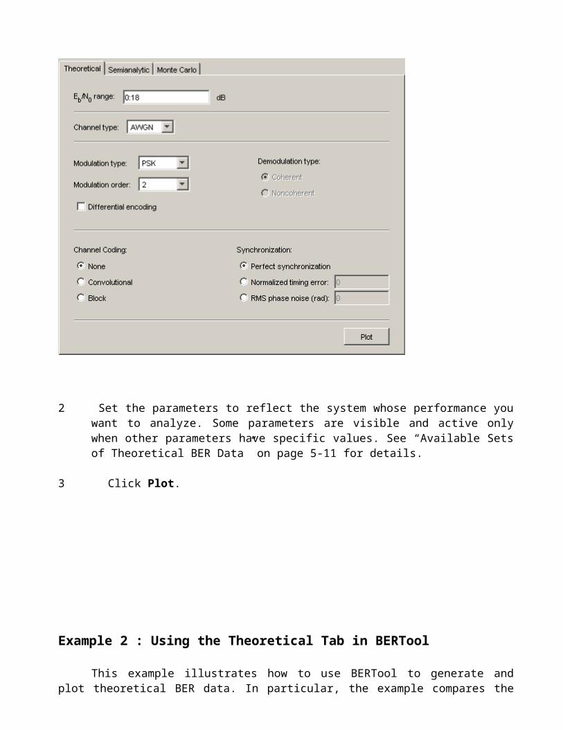
1 Open BERTool, and go to the Theoretical tab.

2 Set the parameters to reflect the system whose performance you want to analyze. Some parameters are visible and active only when other parameters have specific values. See “Available Sets of Theoretical BER Data” on page 5-11 for details.

3 Click Plot.

Example 2 : Using the Theoretical Tab in BERTool

This example illustrates how to use BERTool to generate and plot theoretical BER data. In particular, the example compares the performance of a communication system that uses an AWGN channel and QAM modulation ofdifferent orders.

Running the Theoretical Example

1 Open BERTool, and go to the Theoretical tab.

2 Set the parameters as shown in the following figure.

3 Click Plot.

4 Change the Modulation order parameter to 16, and click Plot. BERTool creates another entry in the data viewer and plots the new data in the same BER Figure window .

5 Change the Modulation order parameter to 64, and click Plot.BERTool creates another entry in the data viewer and plots the new data in the same BER Figure window.

6 To recall which value of Modulation order corresponds to a given curve,click the curve. BERTool responds by adjusting the parameters in the Theoretical tab to reflect the values that correspond to that curve.

7 To remove the last curve fromthe plot (but not fromthe data viewer), clear the check box in the last entry of the data viewer in the Plot column. To restore the curve to the plot, select the check box again.

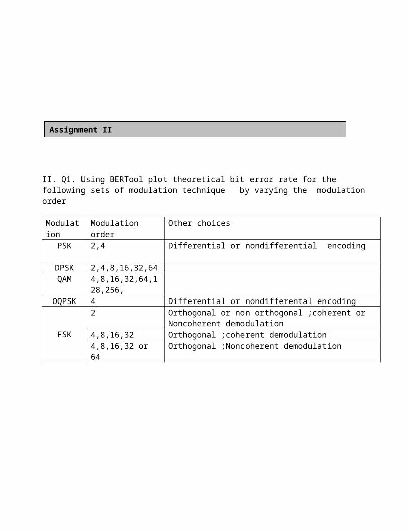
II. Q1. Using BERTool plot theoretical bit error rate for the following sets of modulation technique by varying the modulation order

Assignment II

Modulation Modulation order Other choicesPSK 2,4 Differential or nondifferential encoding

DPSK 2,4,8,16,32,64QAM 4,8,16,32,64,128,256

,OQPSK 4 Differential or nondifferental encoding

FSK

2 Orthogonal or non orthogonal ;coherent or Noncoherent demodulation

4,8,16,32 Orthogonal ;coherent demodulation4,8,16,32 or 64 Orthogonal ;Noncoherent demodulation

Performance Results via the Semianalytic Technique

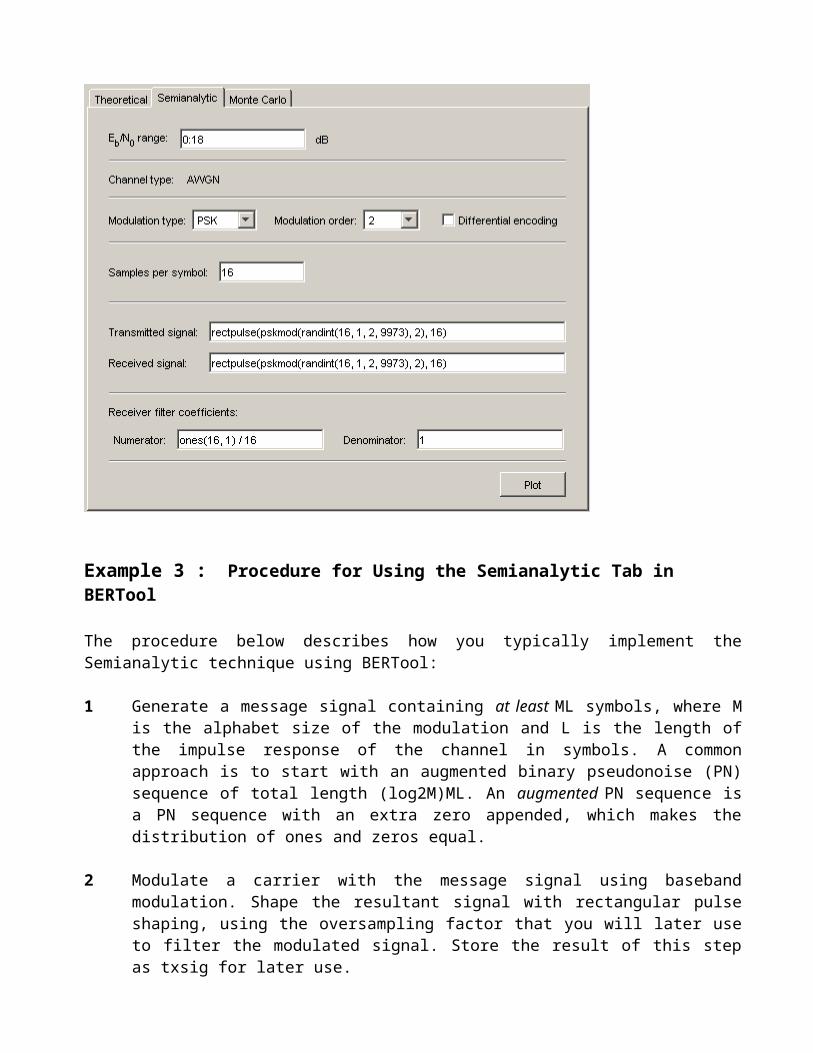
To access the semianalytic capabilities of BERTool, open the Semianalytic tab.

Example 3 :Procedure for Using the Semianalytic Tab in BERTool

The procedure below describes how you typically implement the Semianalytic technique using BERTool:

1 Generate a message signal containing at least ML symbols, where M is the alphabet size of the modulation and L is the length of the impulse response of the channel in symbols. A common approach is to start with an augmented binary pseudonoise (PN) sequence of total length (log2M)ML. An augmented PN sequence is a PN sequence with an extra zero appended, which makes the distribution of ones and zeros equal.

2 Modulate a carrier with the message signal using baseband modulation. Shape the resultant signal with rectangular pulse shaping, using the oversampling factor that you will later use to filter the modulated signal. Store the result of this step as txsig for later use.

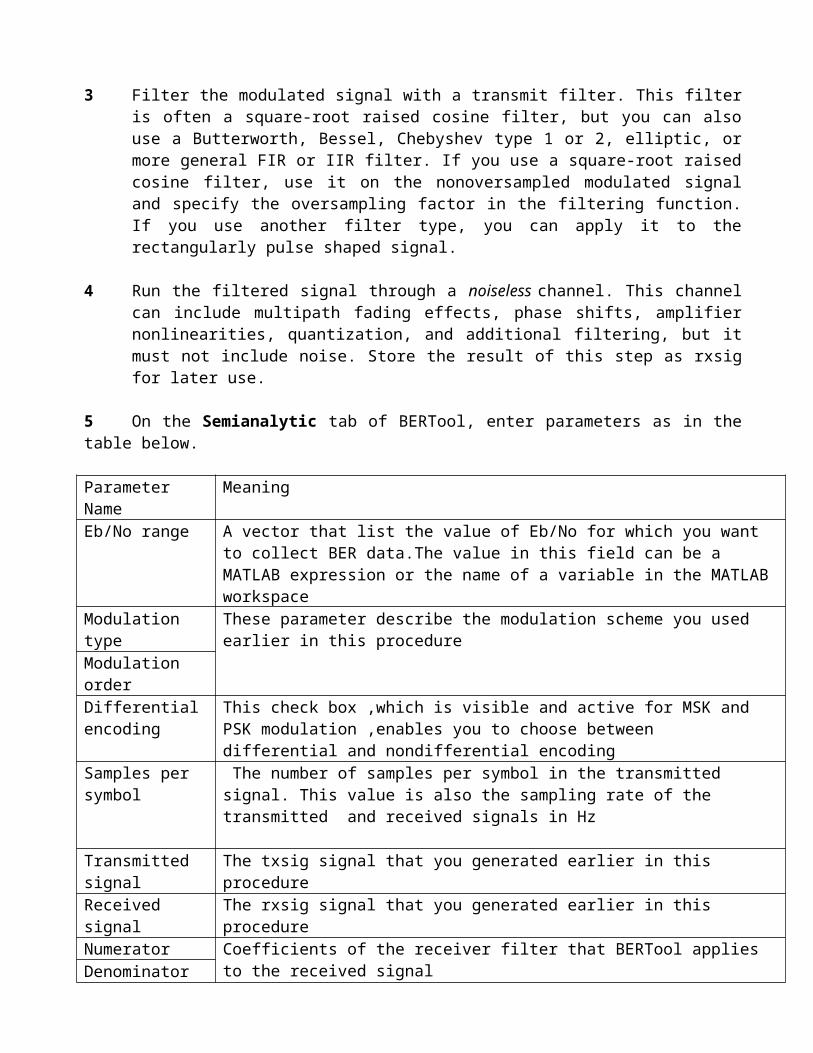
3 Filter the modulated signal with a transmit filter. This filter is often a square-root raised cosine filter, but you can also use a Butterworth, Bessel, Chebyshev type 1 or 2, elliptic, or more general FIR or IIR filter. If you use a square-root raised cosine filter, use it on the nonoversampled modulated signal and specify the oversampling factor in the filtering function. If you use another filter type, you can apply it to the rectangularly pulse shaped signal.

4 Run the filtered signal through a noiseless channel. This channel can include multipath fading effects, phase shifts, amplifier nonlinearities, quantization, and additional filtering, but it must not include noise. Store the result of this step as rxsig for later use.

5 On the Semianalytic tab of BERTool, enter parameters as in the table below.

Parameter Name MeaningEb/No range A vector that list the value of Eb/No for which you want to collect BER data.The

value in this field can be a MATLAB expression or the name of a variable in the MATLAB workspace

Modulation type These parameter describe the modulation scheme you used earlier in this procedureModulation orderDifferential encoding

This check box ,which is visible and active for MSK and PSK modulation ,enables you to choose between differential and nondifferential encoding

Samples per symbol

The number of samples per symbol in the transmitted signal. This value is also the sampling rate of the transmitted and received signals in Hz

Transmitted signal The txsig signal that you generated earlier in this procedureReceived signal The rxsig signal that you generated earlier in this procedureNumerator Coefficients of the receiver filter that BERTool applies to the received signalDenominator

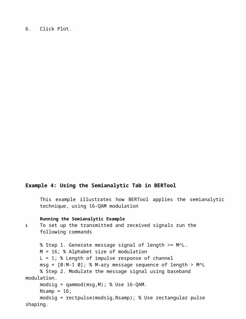
6. Click Plot.

Example 4: Using the Semianalytic Tab in BERTool

This example illustrates how BERTool applies the semianalytic technique, using 16-QAM modulation

Running the Semianalytic Example1 To set up the transmitted and received signals run the following commands

% Step 1. Generate message signal of length >= M^L.M = 16; % Alphabet size of modulationL = 1; % Length of impulse response of channelmsg = [0:M-1 0]; % M-ary message sequence of length > M^L% Step 2. Modulate the message signal using baseband modulation.modsig = qammod(msg,M); % Use 16-QAM.Nsamp = 16;modsig = rectpulse(modsig,Nsamp); % Use rectangular pulse shaping.% Step 3. Apply a transmit filter.txsig = modsig; % No filter in this example% Step 4. Run txsig through a noiseless channel.rxsig = txsig*exp(1i*pi/180); % Static phase offset of 1 degree

2 Open BERTool and go to the Semianalytic tab.3 Set parameters as shown in the following figure.

4 Click Plot.

III F) Running MATLAB Simulations

You can use BERTool in conjunction with your own MATLAB simulation functions to generate and analyze BER data. The MATLAB function simulates the communication system whose performance you want to study. BERTool invokes the simulation for Eb/N0 values that you specify, collects the BER data from the simulation, and creates a plot. BERTool also enables you to easily change the Eb/N0 range and stopping criteria for the simulation.

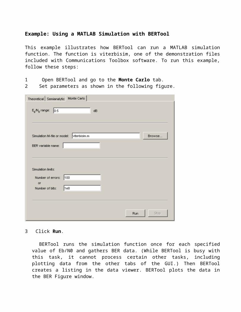
Example: Using a MATLAB Simulation with BERTool

This example illustrates how BERTool can run a MATLAB simulation function. The function is viterbisim, one of the demonstration files included with Communications Toolbox software. To run this example, follow these steps:

1 Open BERTool and go to the Monte Carlo tab. 2 Set parameters as shown in the following figure.

3 Click Run.

BERTool runs the simulation function once for each specified value of Eb/N0 and gathers BER data. (While BERTool is busy with this task, it cannot process certain other tasks, including

plotting data from the other tabs of the GUI.) Then BERTool creates a listing in the data viewer. BERTool plots the data in the BER Figure window.

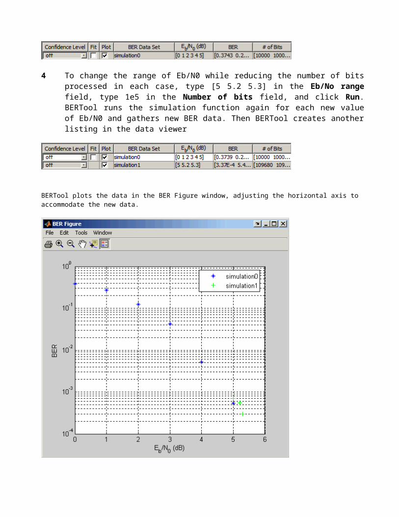
4 To change the range of Eb/N0 while reducing the number of bits processed in each case, type [5 5.2 5.3] in the Eb/No range field, type 1e5 in the Number of bits field, and click Run. BERTool runs the simulation function again for each new value of Eb/N0 and gathers new BER data. Then BERTool creates another listing in the data viewer

BERTool plots the data in the BER Figure window, adjusting the horizontal axis to accommodate the new data.

The two points corresponding to 5 dB from the two data sets are different because the smaller value of Number of bits in the second simulation caused the simulation to end before observing many errors

Part IIISimulink BER calculations

This example starts from a Simulink model originally created as an example in the Communications Blockset Getting Started documentation, and shows how to tailor the model for use with BERTool. The example also illustrates howto compare the BER performance of a Simulink simulation with theoretical BER results.

To prepare the model for use with BERTool, follow these steps, using the exact case-sensitive variable names as shown:

III.Q1. (demo)

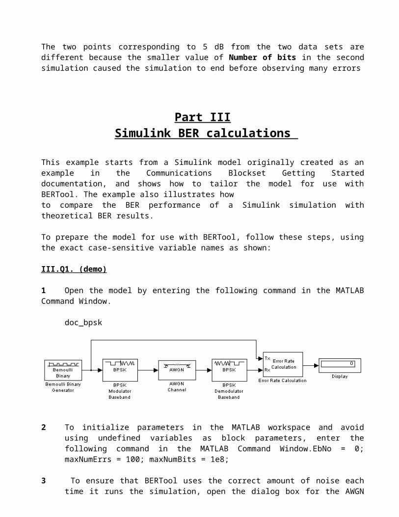
1 Open the model by entering the following command in the MATLAB Command Window.

doc_bpsk

2 To initialize parameters in the MATLAB workspace and avoid using undefined variables as block parameters, enter the following command in the MATLAB Command Window.EbNo = 0; maxNumErrs = 100; maxNumBits = 1e8;

3 To ensure that BERTool uses the correct amount of noise each time it runs the simulation, open the dialog box for the AWGN Channel block by double-clicking the block. Set Es/No to EbNo and click OK. In this particular model, Es/N0 is equivalent to Eb/N0 because the modulation type is BPSK.

4 To ensure that BERTool uses the correct stopping criteria for each iteration, open the dialog box for the Error Rate Calculation block. Set Target number of errors to maxNumErrs, set Maximum number of symbols to maxNumBits, and click OK.

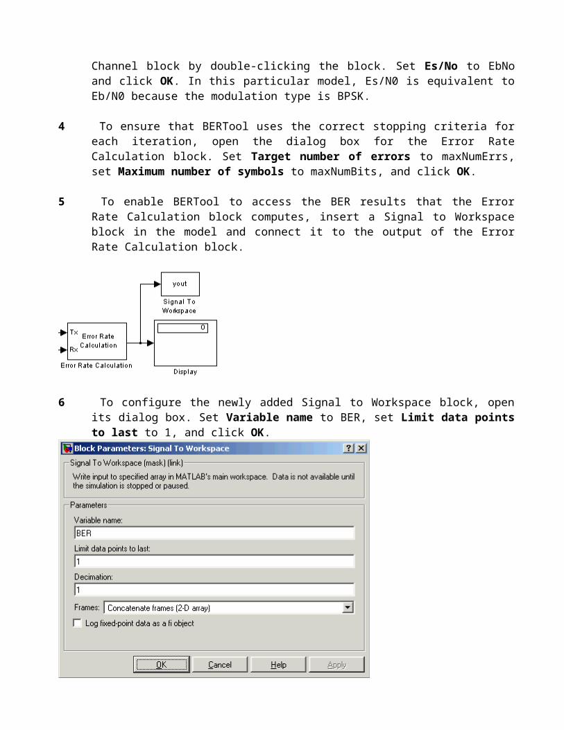
5 To enable BERTool to access the BER results that the Error Rate Calculation block computes, insert a Signal to Workspace block in the model and connect it to the output of the Error Rate Calculation block.

6 To configure the newly added Signal to Workspace block, open its dialog box. Set Variable name to BER, set Limit data points to last to 1, and click OK.

7 (Optional) To make the simulation run faster, especially at high values of Eb/N0, open the dialog box for the Bernoulli Binary Generator block. Select Frame-based outputs and set Samples per frame to 1000.

8 Save the model in a folder on your MATLAB path using the file name bertool_bpskdoc.mdl.

9 Open BERTool and go to the Monte Carlo tab.

10 Set parameters on the Monte Carlo tab as shown in the following figure.

11 Click Run.

12 To compare these simulation results with theoretical results, go to the Theoretical tab in BERTool and set parameters as shown below.

13 Click Plot.

BERTool plots the theoretical curve in the BER Figure window along with the earlier simulation results.

Repeat III.Q1 for the following models.

III. Q2. Describe the modulation/demodulation and receiver of system, PLOT performance curve.

III. Q3. Describe the modulation/demodulation and receiver of system, PLOT performance curve.

Discussion and Conclusion