Embed Size (px)
Citation preview

doc.: IEEE 802.11-15/1110r0
Amin Jafarian, Newracom1
September 2015
BSS-TXOP
Name Affiliations Address Phone emailAmin Jafarian Newracom [email protected]
Reza Hedayat
Minho Cheong
Young Hoon Kwon
Daewon Lee
Vida Ferdowsi
Yongho Seok

doc.: IEEE 802.11-15/1110r0
Amin Jafarian, Newracom2
September 2015
CCA performance analysis summary
• Summary of the last couple of meetings:– We showed that
1. Reducing the CCA threshold does not really solve the medium reuse issue when the network is crowded
2. There is a lot of medium reuse opportunity for other neighbor STAs even without effecting primary MCS
3. The medium reuse opportunity increases even more if the network gets more crowded
doc.: IEEE 802.11-15/1110r0
Amin Jafarian, Newracom3
September 2015
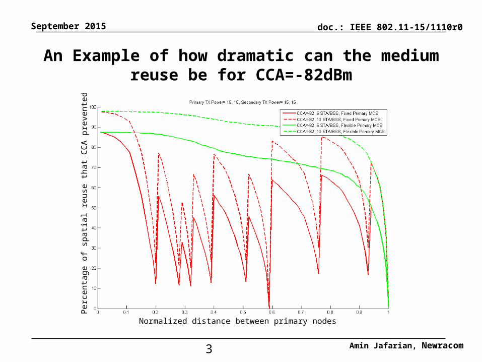
An Example of how dramatic can the medium reuse be for CCA=-82dBm
Normalized distance between primary nodes
Perc
enta
ge o
f spa
tial r
euse
that
CCA
pre
vent
ed

doc.: IEEE 802.11-15/1110r0
Amin Jafarian, Newracom4
September 2015
The group agreed on
We agreed on the following two straw polls:
• A STA is allowed to transmit even if the channel is busy according to Clause 22 if some specific condition is met. One instant of the above condition is limiting the maximum amount of interference caused by the secondary pair transmission on the primary pair receivers.
• Y/N/A:17/1/23
Here we address a framework to facilitate this idea
doc.: IEEE 802.11-15/1110r0
Amin Jafarian, Newracom5
September 2015
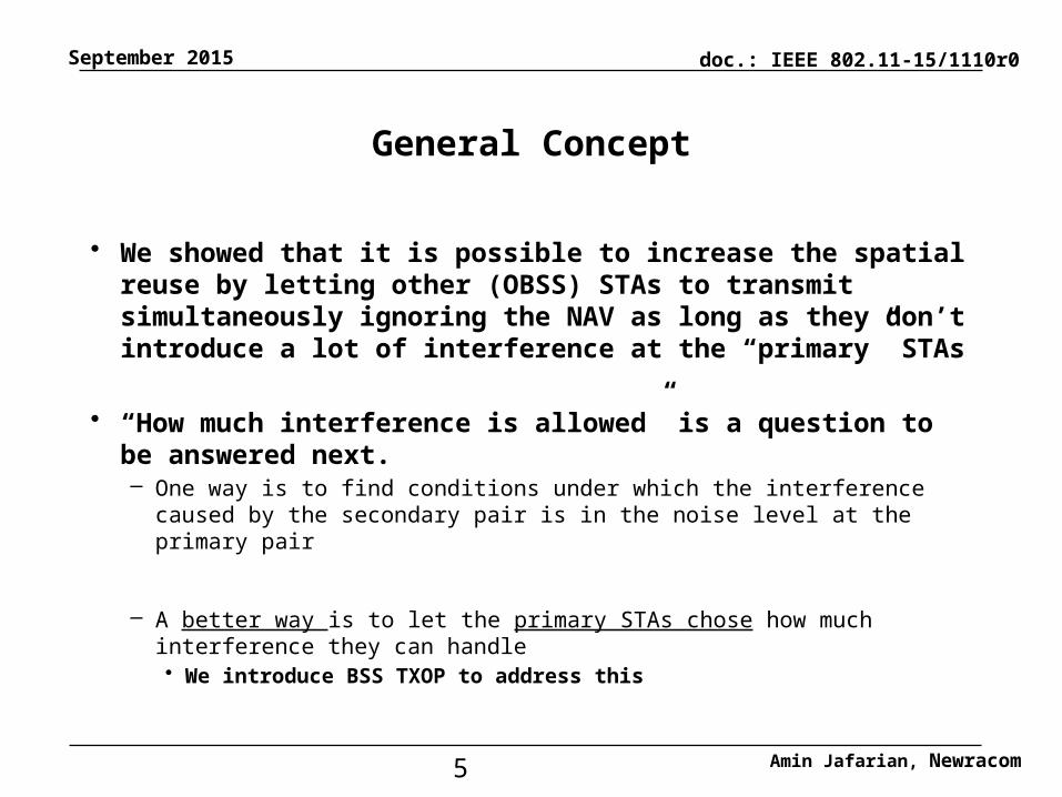
General Concept
• We showed that it is possible to increase the spatial reuse by letting other (OBSS) STAs to transmit simultaneously ignoring the NAV as long as they don’t introduce a lot of interference at the “primary” STAs
• “How much interference is allowed” is a question to be answered next.– One way is to find conditions under which the interference caused by the secondary pair is
in the noise level at the primary pair
– A better way is to let the primary STAs chose how much interference they can handle• We introduce BSS TXOP to address this
doc.: IEEE 802.11-15/1110r0
Amin Jafarian, Newracom6
September 2015
BSS TXOP
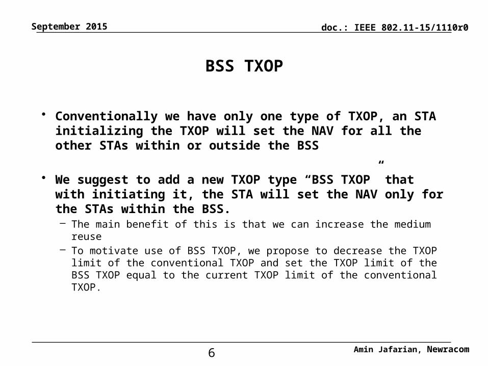
• Conventionally we have only one type of TXOP, an STA initializing the TXOP will set the NAV for all the other STAs within or outside the BSS
• We suggest to add a new TXOP type “BSS TXOP” that with initiating it, the STA will set the NAV only for the STAs within the BSS.– The main benefit of this is that we can increase the medium reuse– To motivate use of BSS TXOP, we propose to decrease the TXOP limit of the conventional
TXOP and set the TXOP limit of the BSS TXOP equal to the current TXOP limit of the conventional TXOP.

doc.: IEEE 802.11-15/1110r0
Amin Jafarian, Newracom7
September 2015
BSS TXOP used case
STA A1 (BSS1)
STA B2 (BSS2)
STA B1 (BSS2)
STA A2 (BSS1)
Con
vent
iona
l TX
OP
Set
the
NA
V f
or
Eve
rybo
dy w
ithi
n R
ange
BSS
TX
OP
Set the NAV within BSS only
BSS
TX
OP
Set the NAV within BSS only
Set the NAV within BSS
only
BSS
TX
OP
Set the NAV
within BSS onlyB
SS T
XO
P

doc.: IEEE 802.11-15/1110r0
Amin Jafarian, Newracom8
September 2015
How helpful
• BSS TXOP can significantly improve the spatial reuse if the primary pairs are located very close to each other and the secondaries are located further– Apartment/ hotel scenario
• In this case, the primary don’t really need to set the NAV for OBSS STAs and it can use the BSS-TXOP
• Secondaries are also in the same situation and can switch to the BSS-TXOP
• If one of the STAs observed a lot of collision, it can switch back to the Conventional TXOP

doc.: IEEE 802.11-15/1110r0
Amin Jafarian, Newracom9
September 2015
Summary
• In a network of 40 STAs, there is a chance of >50% that some other pair of STAs could share the medium with the CCA holder but the CCA prevents that (this is the case when CCA threshold is -72dbm).– For CCA threshold of -82db, it is more than 95% chance
• We propose a new TXOP that motivates not setting the NAV for OBSS and promotes spatial reuse

doc.: IEEE 802.11-15/1110r0
Amin Jafarian, Newracom10
September 2015
Straw Poll
Do you agree with the definition of BSS-TXOP that can be used to set the NAV for the BSS STAs only.
– Y/N/A:

doc.: IEEE 802.11-15/1110r0
Amin Jafarian, Newracom11
September 2015
Back Up slides From 318r1 and 588r0
doc.: IEEE 802.11-15/1110r0
Amin Jafarian, Newracom12
September 2015
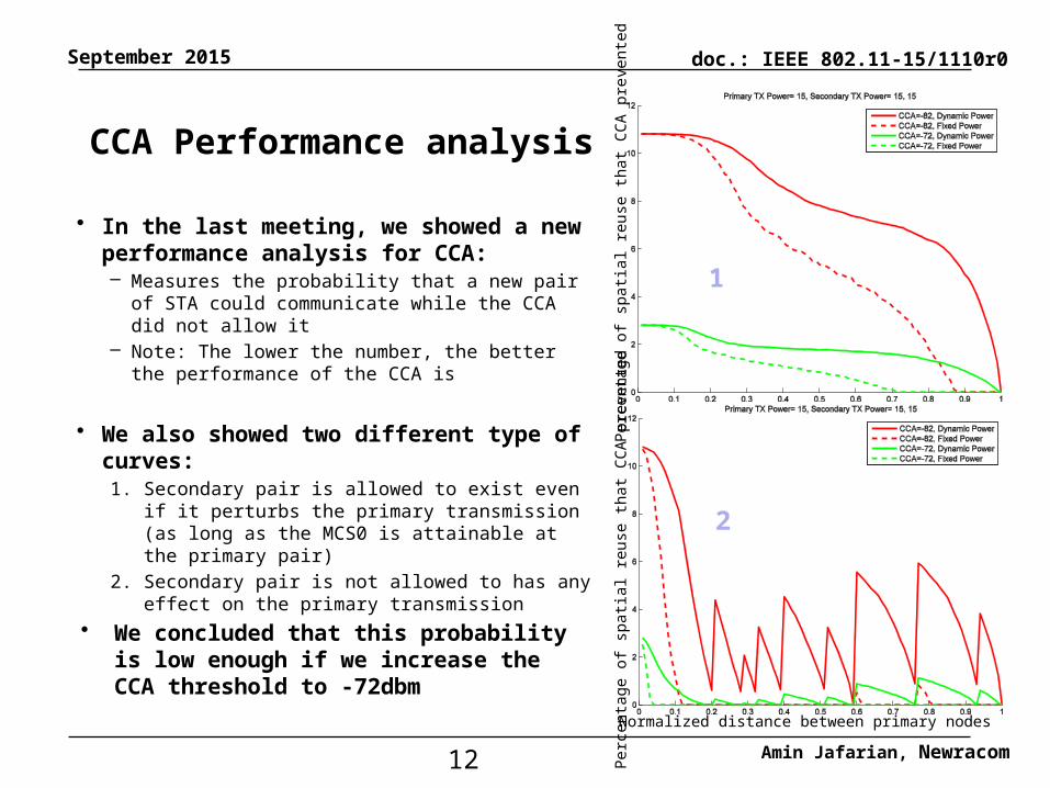
CCA Performance analysis
• In the last meeting, we showed a new performance analysis for CCA:– Measures the probability that a new pair of STA
could communicate while the CCA did not allow it– Note: The lower the number, the better the
performance of the CCA is
• We also showed two different type of curves:1. Secondary pair is allowed to exist even if it
perturbs the primary transmission (as long as the MCS0 is attainable at the primary pair)
2. Secondary pair is not allowed to has any effect on the primary transmission
• We concluded that this probability is low enough if we increase the CCA threshold to -72dbm
1
2
Normalized distance between primary nodes
Perc
enta
ge o
f spa
tial r
euse
that
CCA
pre
vent
edPe
rcen
tage
of s
patia
l reu
se th
at C
CA p
reve
nted
doc.: IEEE 802.11-15/1110r0
Amin Jafarian, Newracom13
September 2015
What if there are multiple Secondary STAs?
• In a crowded network it is very likely that there are multiple BSS around the BSS that sets the CCA
• In each BSS, there are multiple STAs that the BSS AP could potentially communicate with during the CCA
• What is the probability that at least one AP among all the neighbor BSS could communicates with at least one of its STAs, but the CCA did not permit?– We will simulate this for two CCA levels as before
doc.: IEEE 802.11-15/1110r0
Amin Jafarian, Newracom14
September 2015
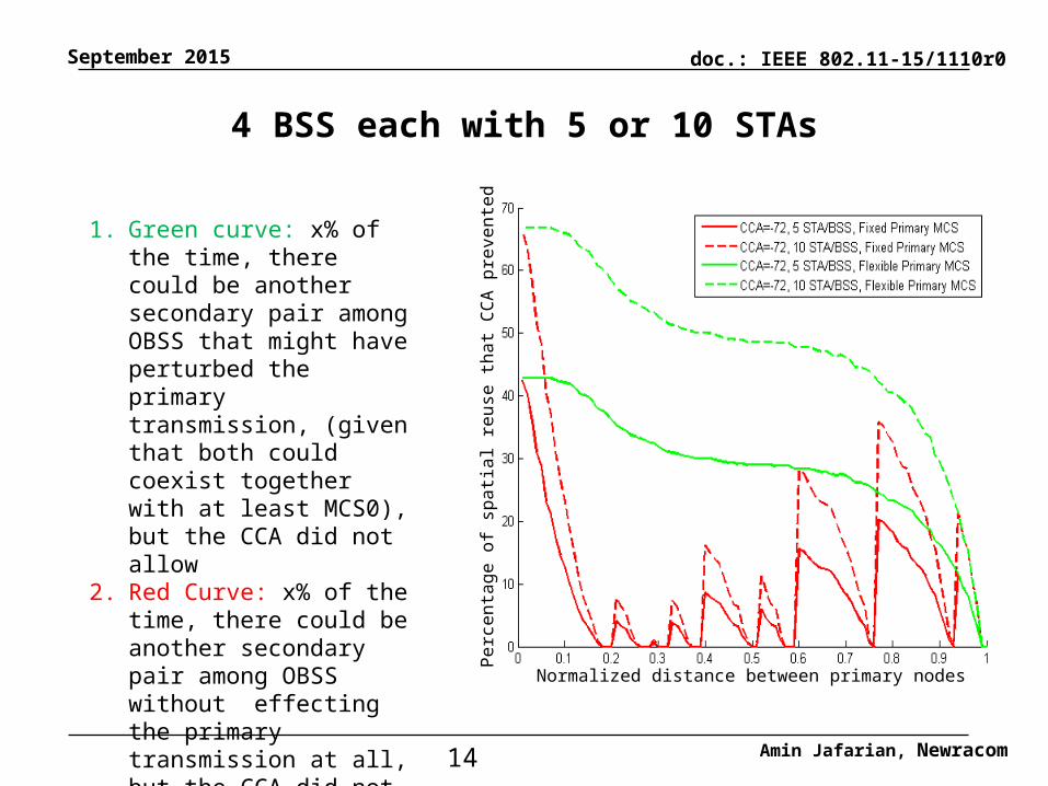
4 BSS each with 5 or 10 STAs
1. Green curve: x% of the time, there could be another secondary pair among OBSS that might have perturbed the primary transmission, (given that both could coexist together with at least MCS0), but the CCA did not allow
2. Red Curve: x% of the time, there could be another secondary pair among OBSS without effecting the primary transmission at all, but the CCA did not allow
Normalized distance between primary nodes
Perc
enta
ge o
f spa
tial r
euse
that
CCA
pre
vent
ed
doc.: IEEE 802.11-15/1110r0
Amin Jafarian, Newracom15
September 2015
Evaluate CCA protocol
Conventional way to evaluate CCA protocols1. Consider a few specific scenarios
• Fix location of STAs/APs in each scenario2. Compute the average medium efficiency gain/loss due to the proposed CCA per
scenario and compare it with the baseline CCA.
• Potential Issues:
1. In each Scenario, the evaluation results can be extremely STA locations dependent
– There might be many more locations that the proposed CCA does not provide any gain– There might be many locations that the gain is higher
2. What is a good definition for gain can be debatable and the result can totally change depends on definition of the gain
– Weighted sum-rate (not fair to the CCA originator)– Maximum achievable rate (not fair to the CCA originator)

doc.: IEEE 802.11-15/1110r0
Amin Jafarian, Newracom16
September 2015
Proposed Evaluation Criteria
To address the previous issues, we propose the following way to evaluate CCA:
1. For an specific scenario, and the proposed CCA, consider many joint locations for all the STAs in the network
2. For each of the locations, compute the event if a simultaneous transmission was possible but the proposed CCA did not allow
3. Compute the percentage number of joint locations (average cases) that #2 was satisfied1. The lower the number is, the better the proposed CCA performed
2. The same thing can be done for the current CCA regime and we can compare the result to see how much gain the proposal provided
The simultaneous transmission could have no additional conditions:Gain definition 1: both transmissions were possible by at least the lowest MCS– Note that this provides an upper bound on the performance of the CCA. But it is not fair for the CCA originator
Or under the condition that the secondary transmission does not hurt the CCA originator’s transmissionsGain definition 2: the secondary transmission was possible with at least the lowest MCS while the original transmission does not change its MCS level– Note 1: that this is the best performance that one can expect from a CCA regime and what we believe is the correct definition of
medium efficiency and fairness in this scenario.– Note 2: while we believe it is very difficult to propose a CCA regime to accomplish this, in our examples, by providing some side
information to the transmitters, we will put a figure on this gain.
doc.: IEEE 802.11-15/1110r0
Amin Jafarian, Newracom17
September 2015
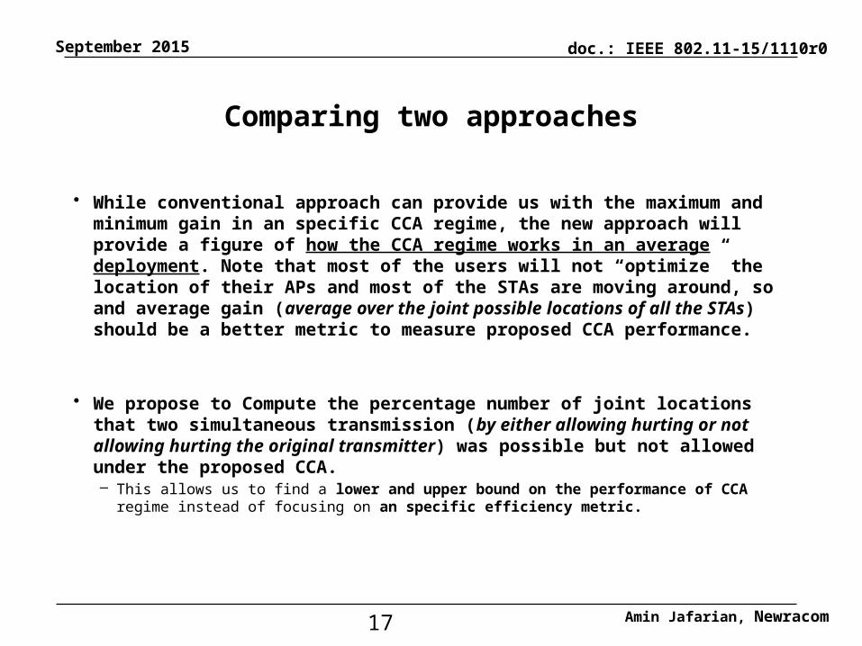
Comparing two approaches
• While conventional approach can provide us with the maximum and minimum gain in an specific CCA regime, the new approach will provide a figure of how the CCA regime works in an average deployment. Note that most of the users will not “optimize” the location of their APs and most of the STAs are moving around, so and average gain (average over the joint possible locations of all the STAs) should be a better metric to measure proposed CCA performance.
• We propose to Compute the percentage number of joint locations that two simultaneous transmission (by either allowing hurting or not allowing hurting the original transmitter) was possible but not allowed under the proposed CCA.– This allows us to find a lower and upper bound on the performance of CCA regime instead of
focusing on an specific efficiency metric.

doc.: IEEE 802.11-15/1110r0
Amin Jafarian, Newracom18
September 2015
Simple Scenario
• We will show a few example of two different CCA regimes under a very simple scenario and assumptions:– We consider a very simple outdoor scenario, no shadowing, no multipath
– Two BSS:
• Primary: This is the CCA originator, we assume the STA started the NAV is the AP in the primary BSS but the same idea goes through if it is a non-AP STA
• Secondary: This is the BSS close to the primary CCA– The transmitter of the secondary BSS is located in the area that is blocked by the existing CCA rules (received power at the transmitter of secondary is
greater than the proposed CCA threshold)– We will calculate the percentage of scenarios (locations) under which there could be a secondary transmission
– Because of symmetry we will fix the location of primary pair and change the secondary pair locations
• We find the percentage of locations that the secondary transmission could exist but it is not allowed as a function of normalized distance of Primary TX and RX (normalized such that the maximum distance for MCS0 being 1).
– We modify the TX powers at each STA and plot the result for each set of TX power.
– For MCS calculations, we used a simple mapping of received SINR to MCS at each receiver. We considered RX sensitivity =-88dbm, and the minimum SINR=4db that maps to MCS0.
– Data Packet Assumptions: Primary Transmitter has a very long packet in the air (more than the duration needed for the secondary packet to be transmitted)
doc.: IEEE 802.11-15/1110r0
Amin Jafarian, Newracom19
September 2015
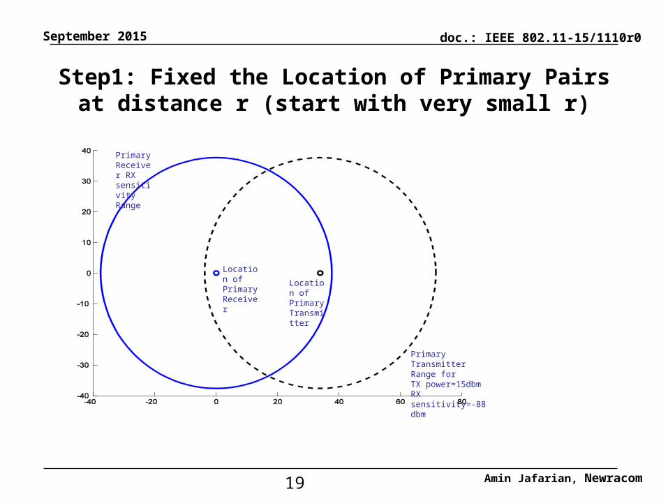
Step1: Fixed the Location of Primary Pairs at distance r (start with very small r)
Location of Primary Receiver
Location of Primary Transmitter
Primary Receiver RX sensitivity Range
Primary Transmitter Range for TX power=15dbmRX sensitivity=-88 dbm

doc.: IEEE 802.11-15/1110r0
Amin Jafarian, Newracom20
September 2015
CCA Coverage
CCA coverage of the ongoing transmission
doc.: IEEE 802.11-15/1110r0
Amin Jafarian, Newracom21
September 2015
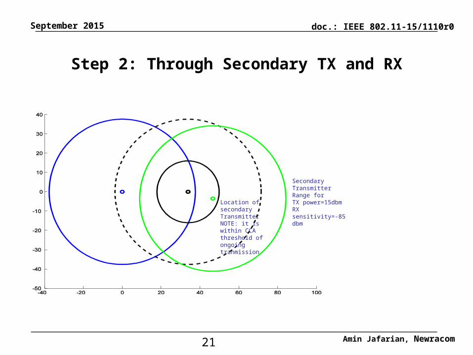
Step 2: Through Secondary TX and RX
Location of secondary TransmitterNOTE: it is within CCA threshold of ongoing tranmission
Secondary Transmitter Range for TX power=15dbmRX sensitivity=-85 dbm

doc.: IEEE 802.11-15/1110r0
Amin Jafarian, Newracom22
September 2015
Step 3: Compute if two simultaneous transmission is possible
Location of secondary receiverNOTE: it is within the RX range of secondary transmitter
Secondary Receiver Range for TX power=15dbmRX sensitivity=-85 dbm

doc.: IEEE 802.11-15/1110r0
Amin Jafarian, Newracom23
September 2015
Final Steps
Step 4: Repeat step 2 and 3 many times– At the end find the percentage of cases that two simultaneous transmission was possible
Step 5: Change the normalized distance of primary pair to r+delta– Redo the computations
Step 6: Plot the percentage of cases with respect to distance r

doc.: IEEE 802.11-15/1110r0
Amin Jafarian, Newracom24
September 2015
CCA Regimes
Four CCA regimes are considered:
• CCA threshold -72dbm1. Fixed power: Secondary STAs are not allowed to change their TX power
2. Dynamic Power: Secondary STAs are provided with the channel knowledge so that they can compute the optimal transmit power that enables them to communicate without causing much interference to the primary pair if possible at all
• Note that this provides the best possible performance one can expect from dynamic CCA. The goal of this presentation is no to address how this information is provided. It is more along the direction of how much this best information can improve CCA regime
• CCA threshold -82dbm3. Fixed Power
4. Dynamic Power
doc.: IEEE 802.11-15/1110r0
Amin Jafarian, Newracom25
September 2015
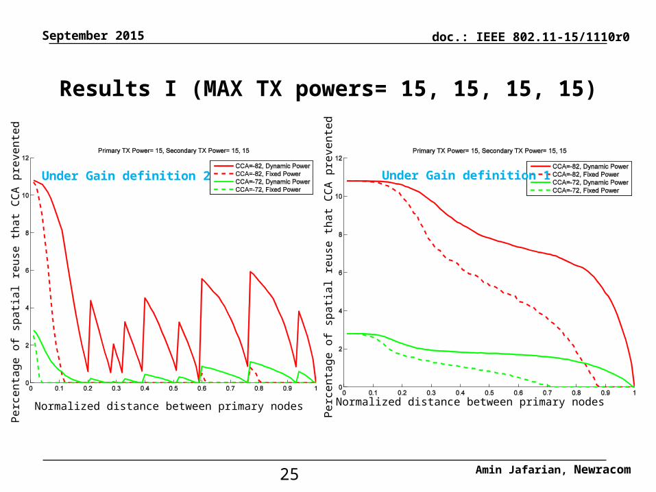
Results I (MAX TX powers= 15, 15, 15, 15)
Under Gain definition 2 Under Gain definition 1
Normalized distance between primary nodes
Perc
enta
ge o
f spa
tial r
euse
that
CCA
pre
vent
ed
Normalized distance between primary nodes
Perc
enta
ge o
f spa
tial r
euse
that
CCA
pre
vent
ed
doc.: IEEE 802.11-15/1110r0
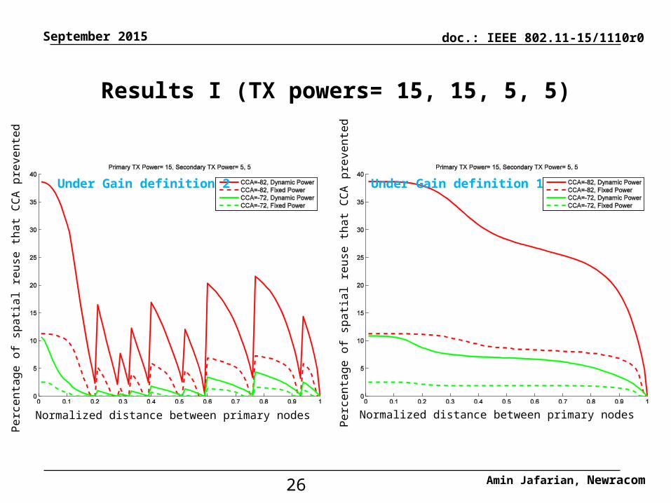
Amin Jafarian, Newracom26
September 2015
Results I (TX powers= 15, 15, 5, 5)
Under Gain definition 2 Under Gain definition 1
Perc
enta
ge o
f spa
tial r
euse
that
CCA
pre
vent
ed
Normalized distance between primary nodes
Perc
enta
ge o
f spa
tial r
euse
that
CCA
pre
vent
ed
Normalized distance between primary nodes

doc.: IEEE 802.11-15/1110r0
Amin Jafarian, Newracom27
September 2015
Interpretation
• In these scenarios dynamic CCA is not needed:– CCA threshold of -72dbm provides very good result, in fact it is less than 5% of locations
that the secondary pair could utilize the medium and CCA prevents that so is there any motivation to propose a more complicated CCA regime for all the STA just to achieve that 5% of locations?
– This is specially the case where the secondary Transmitter is a non-AP STA.