Examensarbete

DOA estimation based on

MUSIC algorithm

Författare: Honghao Tang

Handledare: Sven Nordebo

Examinator: Pieternella Cijvat

Datum: 2014-05-16

Kurskod: 2ED14E, 15 hp

Ämne: Electrical Engineering

Nivå: Bachelor degree

Institutionen för Fysik och Elektroteknik

I

Summary

DOA estimation plays an important role in array signal processing, and has a

wide range of application. In this thesis, I will describe what DOA (Direction of

arrival) estimation is, and give a mathematical model of DOA estimation. Then

estimate DOA based on the MUSIC algorithm, and also give some simulations

with MATLAB to simulate what factors can affect the accuracy and resolution of

DOA estimation when using the MUSIC algorithm.

II

Sammanfattning

DOA uppskattning spelar en viktig roll i array signalbehandling, och har ett brett

användningsområde. I denna uppsats kommer jag att beskriva vad DOA

(Direction of Arrival) uppskattning är, och ge en matematisk modell av DOA

uppskattning. Efter det uppskattar jag DOA baserad på MUSIC-algoritmen, och

ger några simuleringar på MATLAB för att simulera vilka faktorer som kan

påverka noggrannheten och upplösningen av DOA uppskattning när MUSIC

algoritmen används.

III

Abstract

Array signal processing is an important branch in the field of signal processing.

In recent years, it has developed dramatically. It can be applied in such fields as

radio detection and ranging, communication, sonar, earthquake, exploration,

astronomy and biomedicine.

The field of direction of array signal processing can be classified into self-

adaption array signal processing and spatial spectrum, in which spatial spectrum

estimation theory and technology is still in the ascendant status, and become a

main aspect in the course of array signal processing. Spatial spectrum estimation

is focused on investigating the system of spatial multiple sensor arrays, with the

main purpose of estimating the signal’s spatial parameters and the location of the

signal source.

The spatial spectrum expresses signal distribution in the space from all directions

to the receiver. Hence, if one can get the signal’s spatial spectrum, then the

direction of arrival (DOA) can be obtained. As thus, spatial spectrum estimation

is also called DOA estimation.

DOA technology research is important in array signal processing, which is an

interdisciplinary technology that develops rapidly in recent years, especially the

direction of arrival with multiple signal sources, the estimation of coherent signal

sources, and the DOA estimation of broadband signals. DOA estimation has a

wide application prospect in radar, sonar, communication, seismology

measurement and biomedicine.

Over the past few years, all kinds of algorithms which can be used in DOA

estimation have made great achievements, the most classic algorithm among

which is Multiple Signal Classification (MUSIC).

In this thesis I will give an overview of the DOA estimation based on MUSIC

algorithm.

Keywords: DOA estimation, spatial spectrum, MUSIC algorithm.

IV

Preface

The weeks passed, and these two months have been really meaningful for my

thesis. During this period, I had to face many challenges but finally I found some

way to overcome them.

Here I should thank my supervisors Ellie and Sven, they helped me a lot and

taught me a lot.

Honghao Tang

Växjö, June 4th 2014

V

Contents

Summary ....................................................................................................................... I

Sammanfattning .......................................................................................................... II

Abstract ...................................................................................................................... III

Preface ........................................................................................................................ IV

Contents ....................................................................................................................... V

Chapter 1 An Introduction to DOA Estimation ....................................................... 1

1.1 Background and significance........................................................................................ 1

1.2 Overview of the development of Direction of Arrival (DOA) .................................... 2

Chapter 2 Basic Knowledge of DOA Estimation ...................................................... 4

2.1 DOA estimation ............................................................................................................. 4

2.1.1 The structure of spatial spectrum estimation system .......................................... 4

2.1.2 The basic principle of DOA estimation ................................................................. 5

2.2 Common methods for the array signal DOA .............................................................. 6

2.3 Factors affecting DOA estimation results ................................................................... 7

2.5 Other relevant knowledge ............................................................................................. 8

Chapter 3 The MUSIC algorithm ............................................................................ 10

3.1 An introduction to the MUSIC algorithm ................................................................. 10

3.2 The mathematical model of DOA estimation ............................................................ 10

3.3 Eigen decomposition of array covariance ................................................................. 12

3.4 The principle and implementation of MUSIC algorithm ........................................ 14

3.5 Improved MUSIC Algorithm ..................................................................................... 15

Chapter 4 Simulation ................................................................................................. 17

An introduction to MATLAB ........................................................................................... 17

Chapter 5 Existing problems and solutions in MUSIC algorithm ........................ 27

Chapter 6 The future of DOA estimation ................................................................ 29

Chapter 7 Conclusion ................................................................................................ 31

References ................................................................................................................... 32

APPENDIX ................................................................................................................. 34

Appendix 1 MATLAB codes for basic MUSIC algorithm ..................................... 34

VI

1

Chapter 1 An Introduction to DOA Estimation

1.1 Background and significance

Array signal processing has wide applications, such as radar, sonar, medicine,

earthquake, satellite, and communication system. It becomes a hotspot and difficult point

in the signal processing domain [1]. Array signal processing aims at processing signals

received by array antenna, strengthening useful signals, restraining the interference and

noise, while at the same time collecting useful signal parameters. Compared with

traditional signal orientation sensor, sensor array can control the beam flexibly, with a

high signal gain and strong ability for interference. That is the reason why array signal

processing theory can boom in recent decade.

There are two research directions for DOA estimation, self-adaption array signal

processing and spatial spectrum estimation. Self-adaption occurs earlier in literature than

spatial spectrum and has already been used in many practical engineering systems. On

the other hand, though spatial spectrum estimation has developed rapidly and had

abundant references, it is rarely found in practical systems. At present, it is still being

developed.

Spatial spectrum is an important concept in array signal processing theory. It presents the

distribution of signals in every direction in the space. Hence, if one can get the signal’s

spatial spectrum, one can get the direction of arrival (DOA). Consequently, spatial

spectrum estimation can be also called as DOA estimation.

DOA estimation is a key research area in array signal processing and many engineering

applications, such as wireless communications, radar, radio astronomy, sonar,

navigation, tracking of various objects, earthquake, medicine and other emergency

assistance devices that need to be supported by direction of arrival estimation [2]. In

modern society, DOA estimation is normally researched as a part in the field of array

processing, so many works highlight radio direction finding. Over the past ten years,

Wireless Local Area Networks (WLANs) have increased quickly because of its

flexibility and convenience. In order to satisfy the requirements of advanced services, a

high-speed data rate is necessary. Owing to the excessive use of the low end of the

spectrum, people begin to search for the higher frequency bands for more applications.

With higher user density, higher frequency and higher data rate, multipath fading and

cross interference become the main issues. In order to solve these problems and get

higher communication capacity, smart antenna systems are proved to be very effective in

suppression of the interference and multipath signals [1]-[3].

Signal processing in smart antenna systems concentrates on the development of efficient

algorithms for Direction of Arrival (DOA) estimation and adaptive beam forming.

However, there are many limitations if DOA estimation uses a fixed antenna. Antenna

main-lobe beam width is inversely proportional to its physical shape. It is not a practical

option to improve the accuracy of angle measurement in accordance with an increase in

the physical aperture of the receiving antenna. Some systems such as missile seeker or

aircraft antenna have limited physical size, so they are sufficiently wide in beam width of

the main lobe to correspond. They do not have a good resolution and if there are multiple

signals falling in the antenna’s main lobe, it becomes too difficult to distinguish between

them.

2

Using an array antenna system with innovative signal processing instead of a single

antenna can enhance the resolution of the DOA estimation. This array structure provides

spatial samplings of the received waveform. In signal reception and parameter

estimation, a sensor array has better performance than a single sensor.

There are many kinds of super resolution algorithms such as spectral estimation, Bartlett,

Capon, ESPRIT, Min-norm and MUSIC [4]. One of the most popular and widely used

subspace-based techniques to estimate the DOA of multiple signal sources is the MUSIC

algorithm. Large numbers of computations are needed to search for the spectral angle

when using the MUSIC algorithm, so in real applications its implementation can be

difficult. Compared with spectral MUSIC algorithm, the Root-MUSIC method has better

performance with reduced complexity computation. It can only be used in uniform linear

array (ULA) or non-uniform linear array whose arrays are restricted to a uniform grid [6]

[7]. In this thesis, I will focus on the MUSIC algorithm.

1.2 Overview of the development of Direction of Arrival (DOA)

Initially, the Direction of Arrival Estimation estimated the linear spectrum based on the

method of Fourier transform. It mainly included the periodogram method. Because it was

affected by the Rayleigh limit, it could not acquire a high-resolution performance, or

resist the noise, so it did not obtain satisfied performance.

Afterwards, based on the statistical analysis of maximum likelihood spectrum estimation,

which has a high-resolution performance and robust character, people began to pay

attention to this method. However, maximum likelihood estimation needs to search for a

high-dimensional parameter space, which means that abundant calculations are required.

Therefore, it is hard to be put into practice [8]-[10].

In 1967, Burg proposed the maximum entropy estimation method, which opened a

modern research area on spectrum. This method includes maximum entropy, AR（

Autoregressive model）, MA（Moving Average Model）, ARMA（Auto-Regressive

and Moving Average Model）parameter method. All those methods have a high

resolution. Nevertheless, they all need a large amount of calculation and a low

robustness. [9, 10].

When it came to the 1980s, the academic community put forward a series of spectrum

estimations based on decomposition of eigenvalues. All those estimations were

represented by Multiple Signal Classification (MUSIC) and Estimation Signal

Parameters via Rotational Invariance Technique (ESPRIT) [11, 12]. In certain conditions,

MUSIC is a one-dimensional implementation of maximum entropy, which shares the

same character with maximum likelihood method [13, 14]. At that point, MUSIC was better

than any other methods and received more and more appreciation. However, it has a

weakness of heavy computation. ESPRIT arithmetic and its improved arithmetic such as

TLS-ESPRTI, VIA-ESPRIT and GEESE have a high resolution. The most important

thing is that this kind of arithmetic avoids large computation in search of the spectrum,

so it can accelerate the speed of Direction of arrival estimation. However, ESPRIT

arithmetic and its improved arithmetic can be achieved only under some special array

structures, so its application is relatively narrow [15].

In recent years, some normal methods on DOA, like ML, MUSIC, ESPRIT, have ignored

the time characteristic of the signal. Along with the wide application of array signal

3

processing, one signal interferes with other signals in many occasions like in the field of

communications. Therefore, when processing the spatial problem, one should consider

the time-domain problem at the same time. Using useful information in the signal more

sufficiently, researchers think signals can be sampled in the spatial domain and time

domain at the same time. The surplus one dimension to replenish the shortage of spatial

domain information, namely use two dimensions to process array signal and reduce the

restraint of the array structure and improve the arithmetic ability of resistance to noise.

In practice, there is often a coloured noise environment. In recent years people try to use

the array signal processing based on higher-order cumulant, since higher-order cumulant

has a natural blind feature for any Gaussian noise. Based on the cumulative amount, the

algorithm makes the original DOA estimation algorithm expand to Gaussian spatial

coloured noise or non-Gaussian noise spatial coloured and white noise [16].

In array signal processing, when antenna array receives multiple signals which form the

signal source, the signal source may be completely unknown and the transmission

channel is also unknown and time-varying. This unknown feature for the transmission

channel is the main reason to limit the high resolution of DOA. So scholars have put

forward the concept of blind DOA estimation [17]. Blind DOA estimation can estimate the

channel’s characteristics under unknown circumstances, and has broad application

prospects. Adaptive blind signal separation began at the pioneering working by Heruah

and Juttne in 1991. Since then, people have proposed many different algorithms in recent

years. In principle, all these blind separation algorithms can be used for DOA estimation.

Many natural and artificial signals, such as voice, biomedical signals, radar and sonar

signals are typical of non-stationary signals, whose characteristics are limited by duration

and time variation. Considering the nonlinear and non-stationary characteristics in the

actual system, use of artificial neural networks in DOA is the research direction in recent

years [18].

All these methods basically stay in the theoretical and experimental simulation stage,

which is far from actual applications. At present, interferometry is mainly used to

estimate DOA. In a variety of DOA estimations which are based on spatial spectrum

estimation, the MUSIC method has a higher resolution, a moderate amount of

computation, better robustness, and wide application in array structure. In the practical

engineering process, people often choose the MUSIC method in experimental studies,

and thus develop a number of hardware devices. Certain results have been achieved in

the practical process.

4

Chapter 2 Basic Knowledge of DOA Estimation

2.1 DOA estimation

2.1.1 The structure of spatial spectrum estimation system

Spatial spectrum estimation is a specialized signal estimation technology that uses space

arrays to achieve a space signal parameter. The entire spatial spectrum system should be

composed of three parts: the incident signal space, spatial array receiver and parameter

estimation. The space can be divided into three corresponding spaces, namely target

stage, observation stage, and estimation stage [19].

Fig 2.1 The system structure of DOA estimation

The above system architecture is described as follows:

1) Target stage is a stage that consists of signal source parameters and a complex environment.

For the spatial spectrum estimation system, it uses some particular methods to estimate the

unknown parameters of signals which come from this complex target stage.

2) Observation stage is a stage which receives the radiation signals from the target stage. Due

to the complexity of the environment, the received data may contain some signal

characteristics (azimuth, distance, polarization, etc.) and the space environment

characteristics (noise, miscellaneous waves, interference, etc.). In addition, due to the

influence of spatial array elements, the data received also contain some features of space

array element (mutual coupling, channel inconsistent, frequency band inconsistency, etc.).

This observation stage is a multidimensional stage which means that the system receiving

dates are composed of plurality of channels, and the traditional time domain processing

method is usually only used for one channel. Of particularly note is that the channel does

not correspond to the array elements; a spatial channel is formed by several or all of the

synthetic array elements. There is no doubt that certain array elements in the stage may be

contained within different channels.

3) Estimation stage is a stage which uses spatial spectrum estimation techniques (including

array signal processing techniques such as array correction and spatial filtering techniques)

5

to extract the signal character parameters from the complex environment.

Estimation stage is equivalent to the reconstruction of the target stage. The accuracy of

reconstruction is determined by many factors, such as the complexity of the environment,

the mutual coupling of spatial array, different channels, frequency band inconsistency,

etc.

Spatial spectrum expresses the energy distribution of signals in all spatial directions. If

one can get the spatial spectrum of the signal, the direction of arrival (DOA) of the signal

can be obtained, so spatial spectrum estimation is also known as DOA estimation.

2.1.2 The basic principle of DOA estimation

DOA is for the direction of array antenna of the radio wave. If the radio wave received

meets the condition of far field narrowband, it can take the front of the radio wave as a

plane. The angle between the array normal and the direction vector of the plane wave is

the Direction of arrival (DOA).

The estimated target of DOA gives N snapshots data: X (1)…X (N), using an algorithm

to estimate the value of multiple signals’ DOA (θ).

For generally far and wide signals, a wave-way difference exists when the same signal

reaches different array elements. This wave-way difference leads to a phase difference

between the arrival array elements. Using the phase difference between the array

elements of the signal one can estimate the signal azimuth, which is the basic principle of

DOA estimation [20].

Figure 2.2 The principle of DOA estimation

For instance, Fig. 2.2 considers two array elements,

d is the distance between the array elements,

c is the speed of light,

θ is the incident angle of the far field signal,

τ is the time delay of the array element.

The signal received by the antenna due to the path difference is

6

τ=ⅆ sin 𝜃

𝑐, (2.1)

thus one can obtain the phase difference between the array elements as

𝜑 =e-jωτ=e-jωⅆ sin 𝜃

𝐶=ⅇ

−j2𝜋ⅆ sin 𝜃

𝜆𝑓0𝑓, (2.2)

where fo is the centre frequency. For narrow band signals, the phase difference is

𝜑 = ⅇ−𝑗2𝜋ⅆ sin 𝜃

𝜆 , (2.3)

where λ is the wavelength of the signal. Therefore, if the time delay of the signal is

known, the direction of the signal can be gained according to Formula (2.1), which is the

basic principle of spatial spectrum estimation techniques.

In this thesis, the following assumptions are used:

1) Point source assumption. Assume that the signal source is a point source, when looking

from the array signal source, the opening angle is zero, and thus the signal source relative

to the direction of the array is determined uniquely.

2) Narrowband signal hypothesis. That means that the signal bandwidth is far less than the

reciprocal of the signal wave propagation across the largest diameter time. Meeting the

narrowband assumption is to ensure that all array elements in the array can capture a signal

at the same time.

3) Array assumptions. Assuming the array is located in the far field region of the source, the

wave is projected to the plane wave. Assuming each element is the same lattice element

and the position is accurate, the array element channel and amplitude and phase are

consistent. This assumption guarantees that the array elements and their channel have no

error.

4) Noise assumptions. Assuming the noise between each array element is zero, variance σ2 is

Gaussian white noise, statistical independently between each array noise and statistically

independent between signal and noise.

2.2 Common methods for the array signal DOA

This section describes some common methods for the DOA estimation.

1. Conventional beam forming method

The DOA estimation method was first used in conventional beam forming algorithm. Its

main idea is: In a certain time, make all arrays estimate a certain direction and measure

the output power; for the output power, produce a maximum power of direction that is

needed by DOA estimation [21].

The main shortcoming of the conventional beam forming method is that: all the freedom

degrees in the array are used to form a beam in the desired direction of observation.

When multiple signal sources are incident, the method is limited to the height of the

beam width and the side lobe, so the resolution is low.

7

2. Capon minimum variance method

Capon minimum variance method is a beam forming technique for the purpose of

enhancing the effect of conventional methods [22]. Conventional beam forming methods

have a defect: when there are multiple signal sources, spatial spectrum estimation

includes the signal source power not only in the estimation direction but also in other

directions. And Capon method reduces the influence of interference by minimizing the

total output power, and thus estimates the direction of the wave.

Compared with conventional beam forming algorithm, the Capon method has greatly

improved resolution [23]. However, the Capon method has obvious shortcomings: if the

other signal’s incident direction is close to the interest signal’s incident direction, the

Capon method will make many errors. It needs to calculate the matrix inversion. When

the number of array elements is large, it needs correlation calculation. The ability to

distinguish is decided by the array geometry and SNR.

3. Eigenspace algorithm

Although the classical beam forming method is usually very effective and frequently

used, these methods have essential limitation in terms of resolution, by the array aperture

limit. Most of these limitations are due to the model structure of input signal. Schmitt

derived the completely geometric solution of DOA estimation without considering the

noise situation, and promoted this geometric solution, finally obtaining a reasonable

approximate solution when noise existed and creating a precedent for the eigenspace

algorithm. This algorithm is later developed into MUSIC algorithm. Except for MUSIC

algorithm, the formation of eigenspace algorithm is mainly due to rotational invariance

techniques by means of signal parameters estimation, which was proposed by Roy. It is

called the ESPRIT algorithm [24].

There are two properties when eigenspace algorithm mainly uses an array of received

data covariance matrix R.

1) Expansion space of feature vectors can be decomposed into two orthogonal subspaces, the

signal subspace (expansion by the larger eigenvector corresponding to the larger

eigenvalue) and the noise subspace (expansion by the smaller eigenvector corresponding

to the smaller eigenvalue)

2) The direction vector from the signal source is orthogonal with the noise subspace.

2.3 Factors affecting DOA estimation results

DOA estimation results can be affected by many factors, not only related to the source of

the incoming signal, but also related to the actual application environment [25]. Here are a

few important influential factors, and in Chapter 4, some simulation experiments will be

conducted to study how to affect the DOA estimation results.

1 Number of array elements

The number of array elements in basic arrays can affect the estimation performance for

super resolution algorithm. Generally speaking, if array parameters are the same, the

more number of array elements, the better estimation performance for super resolution

algorithm.

8

2 Snapshots

In the time domain, the number of snapshots is defined as the number of samples. In the

frequency domain, the number of snapshots is defined as the number of time sub-

segments of discrete Fourier transform (DFT).

3 SNR

Assuming the signal and noise have a flat pass band power spectral density, and the

power of signal source is σ2p, noise power isσ2

n, then in this case SNR can be defined as

SNR=20 log (𝜎𝑃

𝜎𝑛), (2.4)

SNR directly affects the performance of super-resolution DOA estimation algorithm. At

a low SNR, super-resolution algorithm performance would drop dramatically. As thus,

how to improve the algorithm under a low SNR is the research focus for the sup-

resolution DOA algorithm [26].

4 The coherence of the signal source

The problem involving coherent sources is a fatal problem for subspace algorithms.

When there is a coherent signal in the signal source, the signal covariance matrix is no

longer for the non-singular matrix. In this case, the original super-resolution algorithm

will fail. Therefore, it will greatly affect the performance of DOA estimation. In addition

to the factors mentioned above, many other factors can affect the performance of DOA

estimation in practical applications, such as the array element amplitude and phase

inconsistencies, mutual coupling between array elements, and the wrong position of

sensors.

2.5 Other relevant knowledge

1 Resolution

In the direction of array, the resolution of the signal source on one direction is directly

related to the rate of change in the vicinity of the array direction vector. In the vicinity of

the rapid changes direction vector, with the change of signal source angle, the snapshots

also change; the corresponding resolution is high. Here a sensitivity characterization

D(θ) is defined,

D(θ)= ‖ⅆ𝑎(𝜃)

ⅆ𝜃‖ ∝ ‖

ⅆ𝜏

ⅆ𝜃‖, (2.5)

where 𝑎(𝜃) is the incident angle of array elements. The larger D(θ) indicates the higher

resolution in this direction.

For uniform linear array (ULA)

D(θ) ∝ cos(𝜃). (2.6)

It shows that signals have a sensitivity that is reduced to half in 60°, so the scope of the

general linear measurement is from -60°to 60°.

2 Hermitian matrixes

Definition: If the complex matrix A satisfies AH=A (H denotes the conjugate transpose),

then A is a Hermitian matrix [30].

9

Let AT be the transpose matrix and �̅� be conjugate matrix respectively, obviously the

necessary and sufficient condition is AT =�̅� for the n-order matrix A= [aij] and Hermitian

matrix, namely

�̅�𝑖𝑗=𝑎𝑖𝑗 （i,j=1,2,…n）. (2.7)

As can be seen from Formula (2.7), the diagonal elements of the Hermitian matrix must

be real numbers.

A Hermitian matrix has the following features：

If A is a Hermitian matrix, then det A is a real number.

If A is a Hermitian matrix, then AT, �̅�, AH are all Hermitian matrixes. When A can be

reversible, A-1 is also the Hermitian.

If A is a Hermitian matrix and k is any real number, then kA is still a Hermitian matrix.

If A, B are all the n-order Hermitian matrixes, then A+B is still a Hermitian matrix.

3 Covariance and covariance matrix

For two-dimensional random variables (X, Y), if E[(X-E(X))(Y-E(Y))] exists, it is called

the covariance of X and Y [31], denoted as COV(X, Y), namely

COV(X, Y)= E[(X-E(X))(Y-E(Y))]=E(XY)-E(X)E(Y). (2.8)

The nature of the covariance is

COV(X, Y)=COV(Y, X);

COV(aX, bY)=abCOV(X, Y), (a, b are constants);

COV(X1+X2, Y)=COV(X1, Y)+COV(X2, Y).

From the definition of covariance, it can be seen that

COV(X, X)=D(X), COV(Y, Y)=D(Y). (2.9)

For n-dimensional random variables (X1,X2,…,Xn), denoted as

Cij=COV(Xi,Xj)

=E[(Xi-E(Xi))(Xj-E(Xj))](i=1,2,…,n), (2.10)

C={Cij} is called covariance matrix for the C (X1, X2, …, Xn).

Covariance matrix C is positive definite (negative definite) symmetric, i.e. CT=C, C ≥ 0.

10

Chapter 3 The MUSIC algorithm

3.1 An introduction to the MUSIC algorithm

Multiple Signal Classification (MUSIC) algorithm was proposed by Schmidt and his

colleagues in 1979 [32]. It has created a new era for spatial spectrum estimation

algorithms. The promotion of the structure algorithm characterized rise and development,

and it has become a crucial algorithm for theoretical system of spatial spectrum. Before

this algorithm was presented, some relevant algorithms directly processed data received

from array covariance matrices. The basic idea of MUSIC algorithm is to conduct

characteristic decomposition for the covariance matrix of any array output data, resulting

in a signal subspace orthogonal with a noise subspace corresponding to the signal

components. Then these two orthogonal subspaces are used to constitute a spectrum

function, be got though by spectral peak search and detect DOA signals.

It is because MUSIC algorithm has a high resolution, accuracy and stability under certain

conditions that it attracts a large number of scholars to conduct in-depth research and

analyses. In general, it has the following advantages when it is used to estimate a signal’s

DOA.

1) The ability to simultaneously measure multiple signals.

2) High precision measurement.

3) High resolution for antenna beam signals.

4) Applicable to short data circumstances.

5) It can achieve real-time processing after using high-speed processing technology.

3.2 The mathematical model of DOA estimation

In order to analyse and derive more conveniently, now assume the following conditions

for the ideal mathematical model of DOA problems.

1) Each test signal source has the same but unrelated polarization. Generally consider

that the signal sources are narrow bands, and each source has the same centre frequency

ω0. The number of testing signal source is D.

2) Antenna array is a spaced linear array which consists of M(M>D) array elements; each

element has the same characteristics, and it is isotropic in each direction.

3) The spacing is d, and the array element interval is not larger than half the wavelength

of the highest signal frequency.

4) Each antenna element in the far field source, namely, an antenna array receiving the

signals coming from the signal source is a plane wave.

5) Both array elements and test signals are uncorrelated; variance σ2 is zero-mean

Gaussian noise nm(t).

6) Each receiving branch has the same characteristics.

11

Figure 3.1 The model of DOA estimation

Let the number of signal sources k (k=1,2,…,D) to the antenna array, the wavefront

signal be Sk(t), as previously assumed, Sk(t) is a narrowband signal, and Sk(t) can be

expressed in the following form

Sk(t) = sk(t)exp{jωk(t)}, (3.1)

where sk(t) is the complex envelope of Sk(t) and ωk(t) is the angular frequency of Sk(t).

As assumed before, all signals have the same centre frequency. So

ωk=ω0= 2𝜋𝑐

𝜆, (3.2)

where c is electromagnetic wave velocity, λ is wave length.

Let the time required by the electromagnetic antenna array dimension be t1. According to

the narrowband assumption, the following approximation is valid,

Sk(t- t1)≈Sk(t). (3.3)

Therefore, the delayed wave front signal is

�̃�𝑘(𝑡 − 𝑡1) = 𝑠𝑘(𝑡 − 𝑡1)exp [𝑗𝜔0(𝑡 − 𝑡1)] = 𝑠𝑘(𝑡)ⅇ𝑥𝑝 [𝑗𝜔0(𝑡 − 𝑡1)]. (3.4)

So use the first array element as reference points. At the moment t, the induction signal

of the array element m (m=1,2,…M) to the k-th signal source in the spaced linear array is

𝑎𝑘𝑠𝑘(𝑡)exp [−𝑗(𝑚 − 1)2𝜋 ⅆ sin 𝜃𝑘

𝜆], (3.5)

where 𝑎𝑘 is the impact of array element m on the signal source k-th. As assumed before,

each array element has no direction, so let ak=1. Θk is direction angle of signal source

k, (𝑚 − 1)ⅆ sin 𝜃𝑘

𝜆 is signal phase difference which is caused by the path difference

between m-th array element and the first array element.

12

Record and measure the noise and all waves from the source, the output signal of the m-

th element is

𝑥𝑚(𝑡) = ∑ 𝑠𝑘(𝑡) exp [−𝑗(𝑚 − 1)2𝜋 ⅆ sin 𝜃𝑘

𝜆] + 𝑛𝑚(𝑡)

𝐷

𝑘=1, (3.6)

where nm(t) is measurement noise; all quantities of labelled m belong to the m-th array

element; all quantities of label k belong to the signal source k. Let

𝑎𝑚(𝜃𝑘) = exp [−𝑗(𝑚 − 1)2𝜋 ⅆ sin 𝜃𝑘

𝜆], (3.7)

be the response function of array element m to signal source k.

Then the output signal of array element m is

𝑥𝑚(𝑡) = ∑ 𝑎𝑚(𝜃𝑘)𝑠𝑘(𝑡) + 𝑛𝑚(𝑡)𝐷𝑘=1 , (3.8)

where 𝑠𝑘(𝑡)is signal strength of signal source k.

This expression can be described by matrices:

X=AS+N, (3.9)

where

X=[x1(t),x2(t),…,xM(t)]T, (3.10)

S=[S1(t),S2(t),…,SD(t)]T, (3.11)

A=[𝑎(𝜃1), 𝑎(𝜃2), … , 𝑎(𝜃𝐷)]T

=[

1 1 ⋯ 1e−𝑗𝜑1 e−𝑗𝜑2 ⋯ e−𝑗𝜑𝐷

⋯ ⋯ ⋯ ⋯e−𝑗(𝑀−1)𝜑1 e−𝑗(𝑀−1)𝜑2 ⋯ e−𝑗(𝑀−1)𝜑𝐷

], (3.12)

with 𝜑𝑘=2𝜋ⅆ

𝜆sin 𝜃𝑘, (3.13)

N=[n1(t),n2(t),…,nM(t)]T. (3.14)

To conduct N sampling point for xm(t), the issue becomes to sample the output signal

xm(t), then estimate the angle 𝜃1, 𝜃2, … , 𝜃𝐷 of signal source DOA from

{xm(i),i=1,2,…,M}.

Thus, it can take the array signal as a superimposed spatial harmonic noise.

3.3 Eigen decomposition of array covariance

For array output x, corresponding calculations can get its covariance matrix Rx:

Rx=E[XXH], (3.15)

13

where H is the conjugate transpose matrix.

As assumed before, signal and noise is uncorrelated, and the noise is zero mean white

noise, so Formula (3.9) can be substituted into Formula (3.5). As thus, the following can

be obtained:

Rx=E[(AS+N)](AS+N)H] (3.16)

=AE[SSH]AH+E[NNH]

=ARsAH+RN,

where Rs=E[SSH] (3.17) is called the signal correlation matrix.

RN=𝜎2𝐼, (3.18)

is the noise correlation matrix, 𝜎2is the power of noise, I is the unit matrix of M*M.

In practical applications, Rx usually cannot be directly obtained and only sample

covariance �̃�𝑥 can be used:

�̃�𝑥 =1

𝑁∑ 𝑥(𝑖)𝑥𝐻(𝑖)

𝑁

𝑖=1, (3.19)

where �̃�𝑥 is the maximum likelihood estimation of Rx. When the number of samples

N→∞, they are the same, but in actual situations there are some errors because of the

limitation of the samples number.

According to the theory that matrix can conduct eigenvalue decomposition, conduct

eigenvalue decomposition to the array covariance matrix. First consider the ideal case,

where noise doesn’t exist:

Rx=ARSAH. (3.20)

For uniform linear array (ULA), the matrix A is a Vandermond matrix which is defined

by Formula (3.12), as long as:

𝜃𝑖 ≠ 𝜃𝑗, i≠j, (3.21)

then, each column is independent. Hence, if Rs is non-singular matrix (Rank(Rs)=D, each

signal source is independent), then:

Rank(ARSAH)=D, (3.22)

since Rx=E[XXH], so:

RxH=Rx, (3.23)

i.e. Rx is a Hermitian matrix, whose eigenvalue is real. Because Rs is positive definite,

ARsAH is semi-positive definite, it has positive eigenvalues D and zero eigenvalues M-D.

Next, consider there is noise

14

Rx=ARSAH+𝜎2𝐼, (3.24)

since 𝜎2>0, Rx is a full rank matrix, Rx has M positive real eigenvalues λ1,λ2,…,λM,

respectively corresponding to the M eigenvectors v1,v2,…,vM. For Rx is a Hermitian

matrix, each eigenvector is orthogonal.

i.e. viHvj=0 i ≠ j, (3.25)

only D eigenvalue is relevant to signals. They are equal to the sum of matrix ARsAH and

every eigenvalue 𝜎2 respectively. That is to say, 𝜎2 is the smallest eigenvalue of R,

which is M-D dimension. For the corresponding eigenvalue vi, i=1,2,…, M, there is still

D related to the signals. In addition, M-D is related to the noise. In the next section, the

nature of characteristic decomposition will be used to determine the source of DOA.

3.4 The principle and implementation of MUSIC algorithm

Characterized by an array of covariance decomposition, the following conclusions can be

drawn:

The eigenvalues of the matrix Rx are sorted in accordance with size, which is

λ1≥λ2 ≥…≥ λM>0, (3.26)

where larger eigenvalues D are corresponding to signal while M-D smaller eigenvalues

are corresponding to noise.

The eigenvalues and eigenvectors which belong to matrix Rx are corresponding to signal

and noise respectively. Therefore, the eigenvalue (eigenvector) of Rx to signal eigenvalue

(eigenvector) and noise eigenvalue (eigenvector) can be divided.

Let λi be the i-th eigenvalues of the matrix Rx, vi is eigenvector corresponding to λi, then:

Rxvi= λivi, (3.27)

let λi=𝜎2 be the minimum of Rx

Rxvi=𝜎2vi i=D+1,D+2,….,M, (3.28)

place (3.24) into (3.28), the following can be acquired

𝜎2vi= (ARSAH+𝜎2𝐼) vi, (3.29)

expand the right side and compare to the left, the following can be obtained

ARSAH vi=0. (3.30)

Because AHA is D*D dimensionally full rank matrix and (AHA)-1 exists, Rs-1 also exists.

From the above, multiply Rs-1(AHA)-1AH on both sides at the same time, then:

Rs-1(AHA)-1AH ARSAH vi=0, (3.31)

so, AH vi=0 i=D+1, D+2,…,M. (3.32)

15

The above equation indicates that the eigenvector corresponding to the noise eigenvalue

(the noise eigenvector) vi is perpendicular with the column vector of the matrix A. Each

row of A is corresponding to the direction of a signal source. That is the starting point of

using noise eigenvector to get the direction of signal source.

Using noise characteristic value as each column, construct a noise matrix En can be

constructed:

En=[VD+1,VD+2,…,VM], (3.33)

to define spatial spectrum Pmu(θ) can be defined:

Pmu(θ)= 1

𝑎𝐻(𝜃)𝐸𝑛𝐸𝑛𝐻𝑎(𝜃)

= 1

∥𝐸𝑛𝐻𝑎(𝜃)∥2

, (3.34)

where the denominator of the formula is an inner product of the signal vector and the

noise matrix. When 𝑎(𝜃) is orthogonal with each column of En, the value of this

denominator is zero, but because of the existence of the noise, it is actually a minimum.

Pmu(θ) has a peak. By this formula, make θ change and estimate the arrival angle by

finding the peak.

The implementation steps of MUSIC algorithm are shown below.

Obtain the following estimation of the covariance matrix based on the N received signal

vector:

𝑅𝑥 =1

𝑁∑ 𝑋(𝑖)𝑋𝐻(𝑖)

𝑁

𝑖=1, (3.35)

to eigenvalue decompose the covariance matrix above

𝑅𝑥 = 𝐴𝑅𝑠𝐴𝐻 + 𝜎2𝐼. (3.36)

According to the order of eigenvalues, take eigenvalue and eigenvector which are equal

to the number of signal D as signal part of space; take the rest, M-D eigenvalues and

eigenvectors, as noise part of space. Get the noise matrix En:

AH vi=0 i=D+1, D+2,…,M, (3.37)

En=[VD+1,VD+2,…,VM], (3.38)

vary θ; according to the formula

Pmu(θ) = 1

𝑎𝐻(𝜃)𝐸𝑛𝐸𝑛𝐻𝑎(𝜃)

. (3.39)

Calculate the spectrum function; then obtain the estimated value of DOA by searching

the peak.

3.5 Improved MUSIC Algorithm

Under the premise of a precise model, MUSIC algorithm can theoretically achieve an

arbitrarily high resolution to DOA [34]. However, for MUSIC algorithm signals, it is

limited to uncorrelated signals. When the source is a correlated signal or a signal with

16

low SNR, the estimated performance of the MUSIC algorithm deteriorates or even

completely loses. This section provides a brief introduction to an improved MUSIC

algorithm, which is proposed by conjugate reconstruction of the data matrix of the

MUSIC algorithm [33].

Make a transformation matrix J, J is an Mth-order anti-matrix, known as the transition

matrix, i.e.

J=[

0 0 … 10 0 … 0… … … …1 0 … 0

], (3.40)

let Y=JX*, where X* is the complex conjugate of X, then the covariance of data matrix

Y is

Ry=E[YYH]=JRX*J. (3.41)

From the sum of Rx and Ry, the reconstructed conjugate matrix can be obtained.

R= Rx+ Ry=𝐴𝑅𝑠𝐴𝐻+J[𝐴𝑅𝑠𝐴𝐻]*J+2𝜎2𝐼. (3.42)

According to matrix theory, the matrices Rx, Ry and R have the same noise subspace. To

conduct characteristic decomposition of R and get its eigenvalue and eigenvector,

according to the estimated number of signal source, separate the noise subspace, and then

use this new noise subspace to construct spatial spectrum and obtain the estimated DOA

value by finding the peak.

17

Chapter 4 Simulation

An introduction to MATLAB

MATLAB is released by the U.S. MathWorks Company. It mainly faces scientific

computing, visualization and interactive program designed for a high-tech computing

environment [27]. It makes numerical analysis, matrix computation, scientific data

visualization, modelling and simulation of nonlinear dynamic systems. Besides, many

other powerful features are integrated in a windows environment which can be used

easily. It provides a comprehensive solution for scientific research, engineering design,

and an effective numerical solution for numerous scientific fields. It is out of the

traditional non-interactive programming languages (such as C, FORTRAN) in some

distance. It represents the highest level of the current international scientific computing

software.

MATLAB is a kind of language, and is also a programming environment. MATLAB

provides a lot of user-friendly tools to manage variables, input and output data, and

generate and manage M files.

Users can type a command in the MATLAB command window. It can also write

applications in the editor using the language it defines. After explaining the language,

process them in a MATLAB environment, and finally returns the results.

The main features of MATLAB [28] are shown below.

1) MATLAB language is simple, compact, easy to use, flexible, and has extremely rich library

functions. The form to write a MATLAB program is free. Using functions from the library

can avoid complicated subroutines programming tasks and compress all unnecessary

programming work. Because library functions are written by experts in this field, users

need not to worry about the reliability of function. It can say that using MATLAB

technology is like standing on the shoulders of experts.

2) Rich operators. Since MATLAB is written in C language, it has the same operators like C

language. Using MATLAB operators flexibly can make the program extremely brief and

easy to understand.

3) MATLAB has both structured control statements (like for loops, while loops, break

statements and if statements) and object oriented programming features.

4) No strict limit for the program and free program design. For example, in MATLAB, users

do not need to predefine matrix when they use it.

5) Well portability procedures. Basically one can run the program without any modification

on various types of computers and operating systems.

6) Powerful graphics function. In both C and FORTRAN languages, graphics are not easy to

draw, but in MATLAB, data visualization is very simple. MATLAB also has strong ability

to edit graphical interface.

7) Powerful toolbox is another feature of MATLAB. MATLAB consists of two parts: a core

part and a variety of optional toolboxes. There are hundreds of core internal functions in

18

the core part. Its toolbox is divided into two categories: functional toolbox and disciplinary

toolbox. Functional toolbox is mainly used to expand the functionality of its symbolic

computation capabilities, modelling and simulation capabilities, text processing and

hardware real-time interactivity. Functional toolbox can be used for a variety of

disciplines. All those toolboxes are written by some high-level experts in the field, so users

do not need to write basic procedures within the scope of their discipline.

8) Open source program. Perhaps it is the most welcomed feature by people. In addition to

the internal function, all MATLAB core files and toolboxes are readable and writeable

source files, so users can modify the source files and add their own files to constitute a

new toolbox.

The drawback of MATLAB is that, compared with other advanced procedures [28], the

processing speed is slow. Because the procedures in MATLAB do not need to do the pre-

treatment, and cannot generate an executable file, in the light of interpretation, the speed

is slow.

In this chapter, I will use MATLAB to do some simulations on the which factors can

affect the DOA estimation.

1 Basic simulation of the MUSIC algorithm for DOA estimation

The first simulation shows how two signals are recognized by the MUSIC algorithm.

There are two independent narrow band signals, the incident angle is 20° and 600

respectively, those two signals are not correlated, the noise is ideal Gaussian white noise,

the SNR is 20dB, the element spacing is half of the input signal wavelength, array

element number is 10, the number of snapshots is 200. The simulation results are shown

in Figure 4.1:

Figure 4.1 basic simulation for MUSIC algorithm

19

As can be seen from Figure 4.1, for the hypothetical situation with two independent

signals, using MUSIC a needle spectrum peak algorithm can be constructed. It may well

estimate the number and direction of the incidence signal, which can be used to estimate

the independent signal source DOA effectively. Under the accurate model, the DOA

estimation can reach any precision; by overcoming the traditional shortcomings of low

precision, it can solve the direction problem with high resolution and high precision in a

multiple signal environment. Hence, high resolution MUSIC algorithm may measure

accuracy, high sensitivity features and have potentially capability with multi-resolution

signals; with better performance and higher efficiency, it can provide high resolution and

asymptotically unbiased DOA estimation, which has a great significance for practical

application.

2 The relationship between DOA estimation and the number of array elements

The second simulation shows there are two independent narrow band signals, the

incident angle is 20° and 600 respectively, those two signals are not correlated, the noise

is ideal Gaussian white noise, the SNR is 20dB, the element spacing is half of the input

signal wavelength, array element number is 10, 50 and 100, the number of snapshots is

200. The simulation results are shown in Figure 4.2:

Figure 4.2 simulation for the relationship between MUSIC algorithm and the number of array elements

As can be seen from Figure 4.2, the dashed line shows the number of array elements are

10, the solid line shows the number of array elements are 50, and the dash-dotted line

20

shows the number of array elements are 100. With other conditions remaining unchanged

and with the increase in the number of array elements, DOA estimation spectral beam

width becomes narrow, the directivity of the array becomes good; that is to say, the

ability to distinguish spatial signals is enhanced. Hence, to get more accurate estimations

of DOA it can increase the number of array elements, but the more the number of array

elements the more the data needs processing; and the more amount of computation, the

lower the speed. From the above figure, when the number of the array elements amounts

to 50 and 100, their beam width is very similar. Therefore, in practice, the number of

elements can be appropriately selected according to specific conditions, and we make

sure of the accuracy of estimates spectrum. By minimizing the waste of resources and

accelerating the speed of operation, work efficiency may improve.

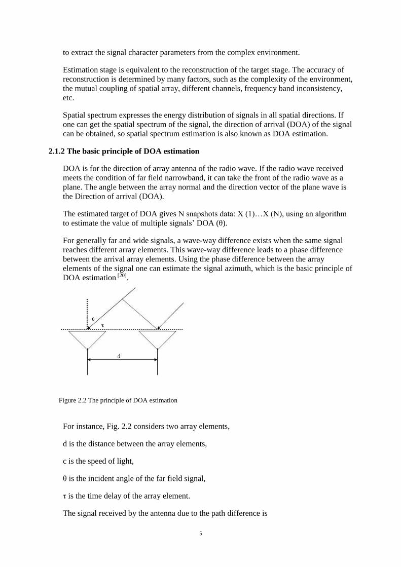
3 The relationship between DOA estimation and the array element spacing

The third simulation shows there are two independent narrow band signals, the incident

angle is 20° and 600 respectively, those two signals are not correlated, the noise is ideal

Gaussian white noise, the SNR is 20dB, array element number is 10, the number of

snapshots is 200, the array spacing is 𝜆 6⁄ , 𝜆 2⁄ , 𝜆. The simulation results are shown in

Figure 4.3:

Figure 4.3 simulation for the relationship between MUSIC algorithm and array element spacing

As can be seen from Figure 4.3, the dashed line shows the array elements spacing is 𝜆 6⁄ ,

the solid line shows the array elements spacing is 𝜆 2⁄ , and the dash-dotted line shows

the array elements spacing is 𝜆. With the other conditions remaining the same, when the

21

array element spacing is not more than half the wavelength, with increasing array

element spacing, the beam width of DOA estimation spectrum becomes narrow, the

direction of the array elements becomes good; that is to say, the resolution of MUSIC

algorithm improves with the increase in the spacing of array element, but, when the

spacing of the array elements is larger than half the wavelength, the estimated spectrum,

except for the signal source direction, shows false peaks, so it has lost the estimation

accuracy. Hence, in practical applications, more attention should be paid to the spacing

of the array elements; element spacing can be increased but must not exceed half the

wavelength, which is a very important point. It is best to set half the wavelength element

spacing.

4 The relationship between DOA estimation and the number of snapshots

The fourth simulation shows how two signals are recognized by the MUSIC algorithm.

There are two independent narrow band signals, the incident angle is 20° and 600

respectively, those two signals are not correlated, the noise is ideal Gaussian white noise,

the SNR is 20dB, the element spacing is half of the input signal wavelength, array

element number is 10, the number of snapshots is5, 50 and 200. The simulation results

are shown in Figure 4.4:

Figure 4.4 simulation for relationship between MUSIC algorithm and the number of snapshots

As can be seen from Figure 4.4, the dashed line shows the number of snapshots are 5, the

solid line shows the number of snapshots are 50 and the dash-dotted line shows the

number of snapshots are 200. With the other conditions remaining unchanged and with

22

the increase in the number of snapshots, the beam width of DOA estimation spectrum

becomes narrow, the direction of the array element becomes good and the accuracy of

MUSIC algorithm is also increased. Hence, the number of sample snapshots can be

expanded to multiply the accuracy of DOA estimation, but the more sample snapshots,

the more the data needs to be processed; the more amount of calculation of MUSIC

algorithm, the lower the speed. So in practical application, we select reasonable sampling

snapshots which ensure the accuracy of DOA estimation, minimize the amount of

computation and accelerating the speed of work and saving resources.

5 The relationship between DOA estimation and SNR

The fifth simulation shows how two signals are recognized by the MUSIC algorithm.

There are two independent narrow band signals, the incident angle is 20° and 600

respectively, those two signals are not correlated, the noise is ideal Gaussian white noise,

the element spacing is half of the input signal wavelength, array element number is 10,

the number of snapshots is 200, the SNR is -20dB, 0dB and 20dB. The simulation results

are shown in Figure 4.5:

Figure 4.5 simulation for the relationship between MUSIC algorithm and SNR

As can be seen from Figure 4.5, the dashed line shows the SNR is -20dB, the solid line

shows the SNR is 0dB and the dash-dotted line shows the SNR is 20dB. With the other

conditions remaining unchanged, with the increase in the number of SNR, the beam

width of DOA estimation spectrum becomes narrow, the direction of the signal becomes

clearer, and the accuracy of MUSIC algorithm is also increased. The value of SNR can

23

affect the performance of high resolution DOA estimation algorithm directly. At low

SNR, the performance of MUSIC algorithm will sharply decline, thus, improving the

estimation performance under low SNR is a main research topic for high resolution DOA

estimation. Some scholars have proposed a DOA estimation algorithm based on

Multistage Weiner filter (MSWF), which uses MSWF to estimate the signal subspace in

the incident direction of the signal, then makes sure the estimate is valid through finding

the minimize across-correlation function after decomposition of MSWF. The signal

subspace and orthogonal noise subspace are estimated, and then the spatial spectrum is

constructed to achieve DOA estimation. Experts have proved in low SNR conditions,

compared with subspace algorithm, MSWF algorithm has better resolution and error

performance. The accuracy of DOA estimation under low SNR has large room for

development and improvement, pending further study.

6 The relationship between DOA estimation and the signal incident angle difference

The sixth simulation shows how two signals are recognized by the MUSIC algorithm.

There are two independent narrow band signals, those two signals are not correlated, the

noise is ideal Gaussian white noise, the SNR is 20dB, the element spacing is half of the

input signal wavelength, array element number is 10, the number of snapshots is 200 and

the incident angle is 5° and 100 and 200respectively. The simulation results are shown in

Figure 4.6:

Figure 4.6 simulation for the relationship between MUSIC algorithm and the incident angle difference

24

As can be seen from Figure 4.6, the dashed line shows the incident angle is 5°, the solid

line shows the incident angle is 10° and the dash-dotted line shows the incident angle is

20°. With the other conditions remaining unchanged and with the increase in incidence

angle difference, the beam width of the DOA estimation spectrum becomes narrow, the

direction of the signal becomes clear and the resolution of MUSIC algorithm is also

increased. When the signal wave angle space is very small, the algorithm cannot

estimate the number of signal sources.

The usual array signal source estimation method conducted under the condition of the

incident angle being large, when the angle difference signal wave direction is relatively

small, are estimated to be ineffective. Some scholars have proposed amendments to the

square root of the Gerschgorin radius estimation method, since it can estimate the source

well when the incident angle difference of signal direction is small. Some kind of method

to estimate the number of signal sources, mostly have certain application conditions,

therefore, to research the real time, steady number of signal sources in line with practical

application and DOA estimation still has much significance.

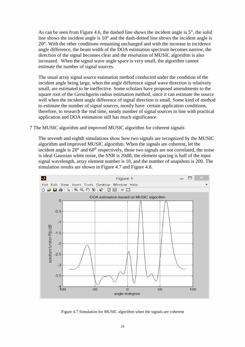
7 The MUSIC algorithm and improved MUSIC algorithm for coherent signals

The seventh and eighth simulations show how two signals are recognized by the MUSIC

algorithm and improved MUSIC algorithm. When the signals are coherent, let the

incident angle is 20° and 600 respectively, those two signals are not correlated, the noise

is ideal Gaussian white noise, the SNR is 20dB, the element spacing is half of the input

signal wavelength, array element number is 10, and the number of snapshots is 200. The

simulation results are shown in Figure 4.7 and Figure 4.8.

Figure 4.7 Simulation for MUSIC algorithm when the signals are coherent

25

Figure 4.8 Simulation for the improved MUSIC algorithm when the signals are coherent

As can be seen from Figure 4.7 and Figure 4.8, for coherent signals, classic MUSIC

algorithm has lost effectiveness, while improved MUSIC algorithm can be better applied

to remove the signal correlation feature, which can distinguish the coherent signals, and

estimate the angle of arrival more accurately. Under the right model, using MUSIC

algorithm to estimate DOA can get any high resolution. But MUSIC algorithm only

focuses on uncorrelated signals; when the signal source is correlation signal, the MUSIC

algorithm estimation performance deteriorates or fails completely. This improved

MUSIC algorithm can make DOA estimation more complete, and have a marked effect

both on theoretical and practical study. For signals to stay coherent, there are many jobs

needed to be done with the realization of DOA estimation, and thus further research is

needed.

Summary

The more the number of array elements, the more the number of snapshots; the more

different between the incident angles, the higher resolution the MUSIC algorithm has.

When the array element spacing is not more than half the wavelength, the resolution of

MUSCI algorithm increases correspondingly with the increase of array element spacing;

however, if the array element spacing is greater than half the wavelength, the spatial

spectrum causes false peaks in other direction except the direction of signal source.

26

When moving low SNR and small difference of incident angle, the performance of the

MUSIC algorithm will decline. Some scholars have proposed some improvements in

algorithm, but these problems are still a hot research topic. Hence, the MUSIC algorithm

still has much room for development, and it is also worth further study.

27

Chapter 5 Existing problems and solutions in MUSIC

algorithm

1 Channel lost pairing

The MUSIC algorithm has many advantages which traditional methods cannot compare

with, but there also exist many limitations when applied in some real systems. One major

reason is that it is more sensitive to error in the system, when the system is in long course

of work, making the ageing characteristics of each channel increasingly serious. With

differences that cause channel mismatch, it will give the performance of MUSIC

algorithm serious trouble.

Correction of inconsistencies in channels can be classified into two types, self-correction

and active correction. Active correction is a relatively mature correction method, as long

as it predicts the direction of the signal source, and it can perform channel amplitude

correction or directly compensate for the algorithm through the general correction

matrix. In terms of self-correction, it is by use of a priori knowledge of the structure of

the array to conduct a pre-process to the received data. In addition, there have existed

many algorithms to improve the robustness of the MUSIC algorithm, such as the

Toeplitz algorithm based on maximum likelihood estimation, but there are special

requirements for the array structure.

2 Underestimation and overestimation of the number of interference source

When the estimated interferers coincide with the number of actual interferers, the

MUSIC algorithm to estimate the direction of interference is accurate. However, when

the number of estimated interferers is more than the number of actual interferers

(overestimation), then in dividing the signal subspace and noise subspace, the MUSIC

space spectrum may possess more peaks than the actual number of interferers, namely

false peaks. Similarly, if the estimated interferers are less than the number of actual

interferers (underestimation), when in dividing the signal subspace and noise subspace,

the dimensionalities in signal subspace will reduce, and some peak in the MUSIC space

will disappear.

The method of source estimation is based on the Akaike[35] information criterion and

minimum description length to determine the number of interference source; it also

cannot consider the number of interference, but the MUSIC algorithm can be used with

weighted modifications.

3 How the coherent interference source influences the algorithm

When the interference sources are coherent, MUSIC algorithms have problems when

determining the number of interferer sources; they cannot divide the signal subspace and

noise subspace, and thus will not be able to estimate the spatial spectrum.

To solve this problem we generally have the following categories: spatial smoothing

technique, signal feature vector technique and frequency smoothing technique. The

spatial smoothing method is the most commonly used method. Spatial smoothing method

requires a specific spatial structure of the array that can be divided into several sub-

28

arrays, then each sub-array can be calculated of the signal correlation matrix. Afterwards,

we do the direction estimation for each sub-array correlation matrix. But its ability of

decorrelation is weak, thus always making much more decrease of the estimated

performance, reducing the effective aperture of the array, increasing the beam width of

the array, and reducing the resolution of the array. It is a dimension reduction process,

and because it requires a special antenna array structure, it is inapplicable for the

reflecting surface of the multi-beam antenna.

The basic idea of frequency-domain smoothing [36] is taking the average of all covariance

matrix of signal power in frequency components. We obtain a non-singular signal

covariance matrix. This method is also applicable to broadband signal source processing.

29

Chapter 6 The future of DOA estimation

DOA estimation theory and technology have become more mature, but there are many

directions which need further research.

1 DOA Estimation Theory

1) Signal model areas. From a rational mathematical model to the study of more

complex and more realistic environment signal model, this would lay a solid

foundation for the application of spatial spectrum theory and algorithm. For example,

consideration of the array signal model causes all kinds of error in the system, the

features of noise in an actual environment, noise and signal correlation and distributed

signal models.

2) New theories and new methods for DOA estimation. On the one hand, focus on the

research of super-resolution DOA estimation theory and algorithm under general

background is still necessary; on the other hand, focus on the research of DOA

algorithm under specific background does not just stay in the research of general

algorithm.

3) Information utilization aspect. Spatial spectrum estimation techniques not only use the

information signal to estimate the spatial orientation parameters of the signal, but also

make full use of the information of the time-domain signal. The different statistical

characteristics of signal and noise as well as other available information is to increase

the signal separability to improve the DOS estimation performance. At present, this

aspect of study concentrates on the use of information, for instance, the use of

Doppler information signals to achieve a multidimensional parameter estimation

dimensionality reduction; utilizing pulse echo signal to improve the signal to noise

ratio; using high-order Cumulant to restrain Gaussian noise; using different signals

Cyclostationarity to separate signals. Meanwhile, the time-domain information for

DOA algorithm is not deep enough, for example, the use of Doppler information

dimensionality reduction will have much impact on DOA estimation; utilizing pulse

information will bring much extent to estimates the signal subspace and noise

subspace; the requirement of high-order cumulants to the number of samples and all

of this requires more in-depth study.

2 Robust DOA estimation

The present spatial spectrum research normally only considers the array amplitude and

phase errors, mutual coupling and position error. The other factors impacting on the

estimated errors are relatively small, such as near-field scattering, electromagnetic

interference and channel bandwidth inconsistency (especially for broadband systems),

non-linear channel amplifier, quantization error and I/Q quadrature sampling errors.

Since array calibration and angle joint estimation of the parameters is an important

direction for robustness of the algorithm, it has a lot of potential to explore. This will

greatly promote the application of spatial spectrum estimation techniques, such as

correction path in multi-array conditions and error correction for broadband arrays.

30

DOA estimation and array calibration can all contribute to the parameters optimization

problem, and therefore, optimizing the function constructor, a fast algorithm for solving

optimization function is worthy of further study.

3 Fast algorithm for DOA estimation

In general, existing high-resolution DOA algorithm still has a relatively large amount of

computation. How to reduce the computational resources, to improve SNR and the

performance of DOA estimation in small snapshots condition and to enhance the real-

time character, robustness and lower implementation complexity will be an important

part of link for spatial spectrum estimation technology. Therefore, the software and

hardware design issues for DOA estimation are bound to be a hot spot. Important aspects

are rapid estimation feature subspace and VLSI implementation in DOA algorithm.

4 Array configuration setting problems

Currently, one-dimensional linear array setup issues has much in-depth research, but

research on two-dimensional array has less work done. This aspect of study is more in

accordance with real environments and targets. Array configuration settings in particular

environments or platforms, the optimal DOA algorithm in particular array setting, and

planar array error on DOA algorithm are important.

5 DOA estimation for the signal form

At present, although the multipath signals, cyclostationary signals, wideband signals, and

distribution signals all have a large amount of research, the research is not mature

enough; in regard to the DOA estimation when multipath signal azimuth is dense, and

the DOA estimation for wideband signal bands is inconsistent. The problem with the

joint between parameters of circulatory angle, and the problems about the parameter

estimation under the condition of variety of signal coexist.

31

Chapter 7 Conclusion

DOA estimation plays an important role in array signal processing, and has a wide range

of applications. In many areas, such as communication, radar, sonar, weather forecasting,

ocean and geological exploration, seismic survey and biomedicine, DOA estimation

problems may occur.

The key to DOA estimation is to use an antenna signal array which is located in different

spatial regions to receive signals from signal sources in different directions. Then the use

of modern signal processing methods may quickly and accurately estimate the direction

of the signal sources. In recent years, a variety of DOA estimation algorithms has

achieved fruitful results, which provides a solid theoretical foundation for practical

application. In this thesis, I have done some research for multiple signal classification

theoretical study and simulation. The main contents and conclusions made in this thesis

are summarized as follows:

In this thesis, by describing DOA estimation, spatial spectrum estimation, and giving a

mathematical model of DOA estimation, an understanding of DOA estimation was

provided. And then the MUSIC algorithm (Multiply Signal Classification) was

implemented in MATLAB, and simulations were performed. From the simulations, it

could be seen that the MUSIC algorithm has a higher resolution the more the number of

array elements, the more the number of snapshots, and the larger the difference between

the incident angles. When the array element spacing is less than half the wavelength, the

MUSIC algorithm resolution increases in accord with the increase of array element

spacing, however, when the array element spacing is greater than the half of wavelength,

except the direction of signal source, other directions appeared as false peaks in the

spatial spectrum. When the signal is coherent, classical MUSIC algorithm has lost

effectiveness, and improved MUSIC algorithm is able to effectively distinguish their

DOA. I implemented the improved MUSIC algorithm for coherent signals. Finally, I

puzzled out some problems by using the MUSIC algorithm in practical application and

giving some solutions on those problems, then looked forward to the future of DOA

estimation as I have mentioned in Chapter 6.

32

References

[1] Haykin S, Reilly J P, Vertaschitsch E. Some Aspects of Array Signal Processing.

IEEE Proc. F, 1992, 139; p1~26.

[2] Haykin S. Array Signal Processing. Prentice Hall. 1985.

[3] S.Unnikersnna Pillai. Array Signal Processing, Springer verlag, 1989.

[4] HongY Wang, Modern Spectrum Estimation, Dongnan University Press, 1990.

[5] Xianci Xiao, Modern Spatial Spectrum Estimation, Haierbin Industry University

Press, 1992.

[6] Xianda Zhang, Zheng Bao, Communication Signal Processing, National Defence

Industry Press, 2000.

[7] Xianda Zhang, Modern Signal Processing, Tsinghua Press, 2000.

[8] Perte Stoica, Maximum Likelihood Method for Direction of Arrival Estimation. IEEE

Trans on ASSP. 1990. Vol. 38(7). P1132~1143.

[9] Michael L. Miller. Maximum Likelihood Narrow-band Direction Finding and EM

Algorithms. IEEE Trans on ASSP. 1990. Vol. 36(10). P1560~1577.

[10] Ziskind I. MAX M, Maximum Likelihood Localization of Multiple Sources by

Alternating Projection. IEEE Trans on ASSP. 1988. Vol. 36(10). P1553~1560.

[11] Ronald D, Degrot. The Constrained MUSIC Problem. IEEE Trans on SP.1993. Vol.

41(3). P1445~1449.

[12] Fuli Richard. Analysis of Min-norm and MUSIC with Arbitrary Array Geometry.

IEEE Trans on AES.1990. Vol. 26(6). P976~985.

[13] Peter Stonica etc. MUSIC Maximum Likelihood and Cramer-Rao Bond, IEEE

Trans on ASSP. 1989. Vol. 37(5). P720~741.

[14] Harry B. Lee etc. Resolution Threshold Beamspace MUSIC for Two Closely

Spaced Emitters. IEEE Trans on ASSP. 1990. Vol. 38(9). P723~738.

[15] M.Gavish etc. Performance Analysis of the VIA ESPRIT Algorithm. IEE-Proc-F.

1993. Vol. 140(2). P123~128.

[16] T J Shan, Wax M. Adaptive beamforming for Coherent Signals and Inference. IEEE

Trans on ASSP. 1985. Vol. 33(4). P527~536.

[17] Zhang XF, Chen C, Li JF, Xu DZ. Blind DOA and Polarization Estimation for

Polarization-sensitive Array using Dimension Reduction MUSIC. Multidimensional

Systems and Signal Processing. Jan, 2014, 25-1. P67~82.

[18] Kim. Y, Ling. H. Direction of Arrival Estimation of Humans with a Small Sensor

Array using an Artificial Neural Network. TX, USA. EMW Publishing. Progress in

Electromagnetics Research B 2011. Vol. 27. pp. 127-49.

[19] Yongliang Wang. Space Spectral Estimation Theory and Algorithm, China.

Tsinghua Press, 2004.

[20] Y.J Huang, Y.W Wang, F.J Meng, G.L Wang. A Spatial Spectrum Estimation

Algorithm based on Adaptive Beamforming Nulling. Piscataway, NJ USA. Jun, 2013. Pp

220-4.

33

[21] Y.N Hou, J.G Huang, X.A Feng. The study on beam-space DOA estimator based on

beam-forming system. Journal of Projectiles, Rockets, Missiles and Guidance, August

2007. Vol. 27. No.3. pp 80-2, 90.

[22] Capon J. High-resolution Frequency-wavenumber Spectrum Analysis. IEEE, 1969.

Vol. 57 Issue 8. P 1408~1418.

[23] Featherstone, W; Strangeways, HJ; Zatman, MA; Mewes, H. A Novel Method to

Improvement the Performance of Capon’s minimum Variance Estimator. London UK.

IEE 1997. Vol. 1. Pp322-5.

[24] Richard Roy, Thonas Kailath. ESPRIT-Estimation of Signal Parameters via

Rotational Invariance Techniques. IEEE Trans on Acoustics Speech and Signal

Processing. July 1989. Vol. 37. No.7 pp 984~995.

[25] L.N Yang. Study of Factors Affecting Accuracy of DOA. Modern Rader. June 2007.

Vol. 29. No. 6. pp 70-3.

[26] C.H Yu, J.L Li. A White Noise Filtering Method for DOA Estimation of Coherent

Signals in Low SNR. Signal Processing. July 2012. Vol. 28. No. 7. pp 957-62.

[27] Gilat Amos. MATLAB: an Introduction with Application. 3rd edition. Wiley; John

Wiley. Cop 2008.

[28] Chapman, Stephen J. Matlab Programming for Engineers. Pacific Grove, Calif,

2000. Chapter 1, section 1. P 2-3.

[30] Hill, David R. Modern Matrix Algebra. Upper Saddle River, NJ, London: Prentice-

Hall International, 2001.

[31] Ben Danforth. Variance-Covariance Matrix. June 1, 2009.

[32] Ralph O, Schmidt. Multiple Emitter Location and signal Parameter Estimation.

IEEE Trans. On Antennas and Propagation, March 1986. Vol. 34. No. 3. pp 276-280.

[33] Debasis Kundu. Modified MUSIC Algorithm for estimating DOA of signals.

Department of Mathematics Indian Institute of Technology, kanour, India. November

1993.

[34] Fei Wen, Qun Wan, Rong Fan, Hewen Wei. Improved MUSIC Algorithm for

Multiple Noncoherent Subarrays. IEEE Signal Processing Letters. Vol. 21, no. 5, May,

2014.

[35] Chen, Xiaoming. "Using Akaike information criterion for selecting the field

distribution in a reverberation chamber." Electromagnetic Compatibility, IEEE

Transactions on 55.4 (2013): 664-670.

[36] Eder, Rafael, and Johannes Gerstmayr. "Special Genetic Identification Algorithm

with smoothing in the frequency domain." Advances in Engineering Software 70 (2014):

113-122.

34

APPENDIX

Appendix 1 MATLAB codes for the basic MUSIC algorithm

%By Honghao Tang

clc

clear all

format long %The data show that as long shaping scientific

doa=[20 60]/180*pi; %Direction of arrival

N=200;%Snapshots

w=[pi/4 pi/3]';%Frequency

M=10;%Number of array elements

P=length(w); %The number of signal

lambda=150;%Wavelength

d=lambda/2;%Element spacing

snr=20;%SNA

D=zeros(P,M); %To creat a matrix with P row and M column

for k=1:P

D(k,:)=exp(-j*2*pi*d*sin(doa(k))/lambda*[0:M-1]); %Assignment matrix

end

D=D';

xx=2*exp(j*(w*[1:N])); %Simulate signal

x=D*xx;

x=x+awgn(x,snr);%Insert Gaussian white noise

R=x*x'; %Data covarivance matrix

[N,V]=eig(R); %Find the eigenvalues and eigenvectors of R

NN=N(:,1:M-P); %Estimate noise subspace

theta=-90:0.5:90; %Peak search

for ii=1:length(theta)

SS=zeros(1,length(M));

for jj=0:M-1

SS(1+jj)=exp(-j*2*jj*pi*d*sin(theta(ii)/180*pi)/lambda);

end

PP=SS*NN*NN'*SS';

Pmusic(ii)=abs(1/ PP);

end

Pmusic=10*log10(Pmusic/max(Pmusic)); %Spatial spectrum function

plot(theta,Pmusic,'-k')

xlabel('angle \theta/degree')

ylabel('spectrum function P(\theta) /dB')

title('DOA estimation based on MUSIC algorithm ')

grid on

35

Appendix 2 MATLAB codes for the relationship between DOA estimation and the

number of array elements

clc

clear all

format long %The data show that as long shaping science and technology

N=200; %Snapshots

doa=[20 60]/180*pi; %DOA

w=[pi/4 pi/3]'; %Frequency

M1=10; %Array elements number

M2=50;

M3=100;

P=length(w); %Number of signal

lambda=150; %Wavelength

d=lambda/2; %Array element spacing

snr=20; %SNR

D1=zeros(P,M1);

D2=zeros(P,M2);

D3=zeros(P,M3);

for k=1:P

D1(k,:)=exp(-j*2*pi*d*sin(doa(k))/lambda*[0:M1-1]); %Assignment matrix

D2(k,:)=exp(-j*2*pi*d*sin(doa(k))/lambda*[0:M2-1]);

D3(k,:)=exp(-j*2*pi*d*sin(doa(k))/lambda*[0:M3-1]);

end

D1=D1';

D2=D2';

D3=D3';

xx=2*exp(j*(w*[1:N])); %Simulate the signal

x1=D1*xx;

x2=D2*xx;

x3=D3*xx;

x1=x1+awgn(x1,snr); %Add Gaussian white noise

x2=x2+awgn(x2,snr);

x3=x3+awgn(x3,snr);

R1=x1*x1'; %Data covariance matrix

R2=x2*x2';

R3=x3*x3';

[N1,V1]=eig(R1); %Find the eigenvalues and eigenvectors of R

[N2,V2]=eig(R2);

[N3,V3]=eig(R3);

NN1=N1(:,1:M1-P); ; %Estimate the noise subspace

NN2=N2(:,1:M2-P);

NN3=N3(:,1:M3-P);

theta=-90:0.5:90;

%%Search the peak

for ii=1:length(theta)

SS1=zeros(1,length(M1));

for jj=0:M1-1

SS1(1+jj)=exp(-j*2*jj*pi*d*sin(theta(ii)/180*pi)/lambda);

end

PP1=SS1*NN1*NN1'*SS1';

36

Pmusic1(ii)=abs(1/ PP1);

end

for ii=1:length(theta)

SS2=zeros(1,length(M2));

for jj=0:M2-1

SS2(1+jj)=exp(-j*2*jj*pi*d*sin(theta(ii)/180*pi)/lambda);

end

PP2=SS2*NN2*NN2'*SS2';

Pmusic2(ii)=abs(1/ PP2);

end

for ii=1:length(theta)

SS3=zeros(1,length(M3));

for jj=0:M3-1

SS3(1+jj)=exp(-j*2*jj*pi*d*sin(theta(ii)/180*pi)/lambda);

end

PP3=SS3*NN3*NN3'*SS3';

Pmusic3(ii)=abs(1/ PP3);

end

Pmusic1=10*log10(Pmusic1/max(Pmusic1)); %Spatial spectrum function

Pmusic2=10*log10(Pmusic2/max(Pmusic2));

Pmusic3=10*log10(Pmusic3/max(Pmusic3));

plot(theta,Pmusic1,'--k','LineWidth',2.0)

hold on

plot(theta,Pmusic2,'k','LineWidth',1.0)

hold on

plot(theta,Pmusic3,'-.k','LineWidth',0.1)

hold off

xlabel('angle \theta/degree')

ylabel('spectrum function P(\theta) /dB')

title('DOA estimation based on MUSIC algorithm')

grid on

37

Appendix 3 MATLAB codes for the relationship between DOA estimation and the

array element spacing

clc

clear all

format long

N=200;

doa=[20 60]/180*pi;

w=[pi/4 pi/3]';

M=10;

P=length(w);

lambda=150;

d=lambda/6;

snr=20;

D=zeros(P,M);

for k=1:P

D(k,:)=exp(-j*2*pi*d*sin(doa(k))/lambda*[0:M-1]);

end

D=D';

xx=2*exp(j*(w*[1:N]));

x=D*xx;

x=x+awgn(x,snr);

R=x*x';

[N,V]=eig(R);

NN=N(:,1:M-P);

theta=-90:0.5:90;

for ii=1:length(theta)

SS=zeros(1,length(M));

for jj=0:M-1

SS(1+jj)=exp(-j*2*jj*pi*d*sin(theta(ii)/180*pi)/lambda);

end

PP=SS*NN*NN'*SS';

Pmusic(ii)=abs(1/ PP);

end

Pmusic=10*log10(Pmusic/max(Pmusic));

plot(theta,Pmusic ,'--k','linewidth',2.0)

hold on

clc

clear all

format long

N=200;

doa=[20 60]/180*pi;

w=[pi/4 pi/3]';

M=10;

P=length(w);

lambda=150;

d=lambda/2;

snr=20;

D=zeros(P,M);

for k=1:P

38

D(k,:)=exp(-j*2*pi*d*sin(doa(k))/lambda*[0:M-1]);

end

D=D';

xx=2*exp(j*(w*[1:N]));

x=D*xx;

x=x+awgn(x,snr);

R=x*x';

[N,V]=eig(R);

NN=N(:,1:M-P);

theta=-90:0.5:90;

for ii=1:length(theta)

SS=zeros(1,length(M));

for jj=0:M-1

SS(1+jj)=exp(-j*2*jj*pi*d*sin(theta(ii)/180*pi)/lambda);

end

PP=SS*NN*NN'*SS';

Pmusic(ii)=abs(1/ PP);

end

Pmusic=10*log10(Pmusic/max(Pmusic));

plot(theta,Pmusic,'k','linewidth',1.0)

hold on

clc

clear all

format long

N=200;

doa=[20 60]/180*pi;

w=[pi/4 pi/3]';

M=10;

P=length(w);

lambda=150;

d=lambda;

snr=20;

D=zeros(P,M);

for k=1:P

D(k,:)=exp(-j*2*pi*d*sin(doa(k))/lambda*[0:M-1]);

end

D=D';

xx=2*exp(j*(w*[1:N]));

x=D*xx;

x=x+awgn(x,snr);

R=x*x';

[N,V]=eig(R);

NN=N(:,1:M-P);

theta=-90:0.5:90;

for ii=1:length(theta)

SS=zeros(1,length(M));

for jj=0:M-1

SS(1+jj)=exp(-j*2*jj*pi*d*sin(theta(ii)/180*pi)/lambda);

end

PP=SS*NN*NN'*SS';

39

Pmusic(ii)=abs(1/ WW);

end

Pmusic=10*log10(Pmusic/max(Pmusic));

plot(theta,Pmusic,'-.k','linewidth',0.1)

hold off

xlabel('angle \theta/degree')

ylabel('spectrum function P(\theta) /dB')

title('DOA estimation based on MUSIC algorithm')

grid on

40

Appendix 4 MATLAB codes for the relationship between DOA estimation and the

number of snapshots

clc

clear all

format long

N1=5;

N2=50;

N3=200;

doa=[20 60]/180*pi;

w=[pi/4 pi/3]';

M=10;

P=length(w);

lambda=150;

d=lambda/2;

snr=20;

D=zeros(P,M);

for k=1:P

D(k,:)=exp(-j*2*pi*d*sin(doa(k))/lambda*[0:M-1]);

end

D=D';

xx1=2*exp(j*(w*[1:N1]));

xx2=2*exp(j*(w*[1:N2]));

xx3=2*exp(j*(w*[1:N3]));

x1=D*xx1;

x2=D*xx2;

x3=D*xx3;

x1=x1+awgn(x1,snr);

x2=x2+awgn(x2,snr);

x3=x3+awgn(x3,snr);

R1=x1*x1';

R2=x2*x2';

R3=x3*x3';

[N1,V1]=eig(R1);

[N2,V2]=eig(R2);

[N3,V3]=eig(R3);

NN1=N1(:,1:M-P);

NN2=N2(:,1:M-P);

NN3=N3(:,1:M-P);

theta=-90:0.5:90;

for ii=1:length(theta)

SS=zeros(1,length(M));

for jj=0:M-1

SS(1+jj)=exp(-j*2*jj*pi*d*sin(theta(ii)/180*pi)/lambda);

end

PP1=SS*NN1*NN1'*SS';

PP2=SS*NN2*NN2'*SS';

PP3=SS*NN3*NN3'*SS';

Pmusic1(ii)=abs(1/ PP1);

Pmusic2(ii)=abs(1/ PP2);

41

Pmusic3(ii)=abs(1/ PP3);

end

Pmusic1=10*log10(Pmusic1/max(Pmusic1));

Pmusic2=10*log10(Pmusic2/max(Pmusic2));

Pmusic3=10*log10(Pmusic3/max(Pmusic3));

plot(theta,Pmusic1,'--k','linewidth',2.0)

hold on

plot(theta,Pmusic2,'-k','linewidth',1.0)

hold on

plot(theta,Pmusic3,'-.k','linewidth',0.1)

hold off

xlabel('angle \theta/degree')

ylabel('spectrum function P(\theta) /dB')

title('DOA estimation based on MUSIC algorithm')

grid on

42

Appendix 5 MATLAB codes for the relationship between DOA estimation and SNR

clc

clear all

format long

N=200;

doa=[20 60]/180*pi;

w=[pi/4 pi/3]';

M=10;

P=length(w);

lambda=150;

d=lambda/2;

snr1=-20;

snr2=0;

snr3=20;

D=zeros(P,M);

for k=1:P

D(k,:)=exp(-j*2*pi*d*sin(doa(k))/lambda*[0:M-1]);

end

D=D';

xx=2*exp(j*(w*[1:N]));

x=D*xx;

x1=x+awgn(x,snr1);

x2=x+awgn(x,snr2);

x3=x+awgn(x,snr3);

R1=x1*x1';

R2=x2*x2';

R3=x3*x3';

[N1,V1]=eig(R1);

[N2,V2]=eig(R2);

[N3,V3]=eig(R3);

NN1=N1(:,1:M-P);

NN2=N2(:,1:M-P);

NN3=N3(:,1:M-P);

theta=-90:0.5:90;

for ii=1:length(theta)

SS=zeros(1,length(M));

for jj=0:M-1

SS(1+jj)=exp(-j*2*jj*pi*d*sin(theta(ii)/180*pi)/lambda);

end

PP1=SS*NN1*NN1'*SS';

PP2=SS*NN2*NN2'*SS';

PP3=SS*NN3*NN3'*SS';

Pmusic1(ii)=abs(1/ PP1);

Pmusic2(ii)=abs(1/ PP2);

Pmusic3(ii)=abs(1/ PP3);

end

Pmusic1=10*log10(Pmusic1/max(Pmusic1));

Pmusic2=10*log10(Pmusic2/max(Pmusic2));

Pmusic3=10*log10(Pmusic3/max(Pmusic3));

43

plot(theta,Pmusic1,'--k','linewidth',2.0)

hold on

plot(theta,Pmusic2,'-k','linewidth',1.0)

hold on

plot(theta,Pmusic3,'-.k','linewidth',0.1)

hold off

xlabel('angle \theta/degree')

ylabel('spectrum function P(\theta) /dB')

title('DOA estimation based on MUSIC algorithm')

grid on

44

Appendix 6 MATLAB codes for the relationship between DOA estimation and the

signal incident angle difference

clc

clear all

format long

N=200;

doa1=[20 25]/180*pi;

doa2=[20 30]/180*pi;

doa3=[20 60]/180*pi;

w=[pi/4 pi/3]';

M=10;

P=length(w);

lambda=150;

d=lambda/2;

snr=20;

D=zeros(P,M);

for k=1:P

D1(k,:)=exp(-j*2*pi*d*sin(doa1(k))/lambda*[0:M-1]);

D2(k,:)=exp(-j*2*pi*d*sin(doa2(k))/lambda*[0:M-1]);

D3(k,:)=exp(-j*2*pi*d*sin(doa3(k))/lambda*[0:M-1]);

end

D1=D1';

D2=D2';

D3=D3';

xx=2*exp(j*(w*[1:N]));

x1=D1*xx;

x2=D2*xx;

x3=D3*xx;

x1=x1+awgn(x1,snr);

x2=x2+awgn(x2,snr);

x3=x3+awgn(x3,snr);

R1=x1*x1';

R2=x2*x2';

R3=x3*x3';

[N1,V1]=eig(R1);

[N2,V2]=eig(R2);

[N3,V3]=eig(R3);

NN1=N1(:,1:M-P);

NN2=N2(:,1:M-P);

NN3=N3(:,1:M-P);

theta=-90:0.5:90;

for ii=1:length(theta)

SS=zeros(1,length(M));

for jj=0:M-1

SS(1+jj)=exp(-j*2*jj*pi*d*sin(theta(ii)/180*pi)/lambda);

end

PP1=SS*NN1*NN1'*SS';

PP2=SS*NN2*NN2'*SS';

PP3=SS*NN3*NN3'*SS';

45

Pmusic1(ii)=abs(1/ PP1);

Pmusic2(ii)=abs(1/ PP2);

Pmusic3(ii)=abs(1/ PP3);

end

Pmusic1=10*log10(Pmusic1/max(Pmusic1));

Pmusic2=10*log10(Pmusic2/max(Pmusic2));

Pmusic3=10*log10(Pmusic3/max(Pmusic3));

plot(theta,Pmusic1,'--k','linewidth',2.0)

hold on

plot(theta,Pmusic2,'-k','linewidth',1.0)

hold on

plot(theta,Pmusic3,'-.k','linewidth',0.1)

hold off

xlabel('angle \theta/degree')

ylabel('spectrum function P(\theta) /dB')

title('DOA estimation based on MUSIC algorithm')

grid on

46

Appendix 7 MATLAB codes The MUSIC algorithm and the improved MUSIC

algorithm for coherent signals

1 The MUSIC algorithm for coherent signals

clc

clear all

format long

N=200;

doa=[20 60]/180*pi;

w=[pi/4 pi/4]';

M=10;

P=length(w);

lambda=150;

d=lambda/2;

snr=20;

D=zeros(P,M);

for k=1:P

D(k,:)=exp(-j*2*pi*d*sin(doa(k))/lambda*[0:M-1]);

end

D=D';

xx=2*exp(j*(w*[1:N]));

x=D*xx;

x=x+awgn(x,snr);

R=x*x';

[N,V]=eig(R);

NN=N(:,1:M-P);

theta=-90:0.5:90;

for ii=1:length(theta)

SS=zeros(1,length(M));

for jj=0:M-1

SS(1+jj)=exp(-j*2*jj*pi*d*sin(theta(ii)/180*pi)/lambda);

end

PP=SS*NN*NN'*SS';

Pmusic(ii)=abs(1/ PP);

end

Pmusic=10*log10(Pmusic/max(Pmusic));

plot(theta,Pmusic,'-k')

xlabel('angle \theta/degree')

ylabel('spectrum function P(\theta) /dB')

title('DOA estimation based on MUSIC algorithm')

grid on

47

2 The improved MUSIC algorithm for coherent signals

clc

clear all

format long

N=200;

doa=[20 60]/180*pi;

w=[pi/4 pi/4]';

M=10;

P=length(w);

lambda=150;

d=lambda/2;

snr=20;

D=zeros(P,M);

for k=1:P

D(k,:)=exp(-j*2*pi*d*sin(doa(k))/lambda*[0:M-1]);

end

D=D';

xx=2*exp(j*(w*[1:N]));

x=D*xx;

x=x+awgn(x,snr);

R=x*x';

J=fliplr(eye(M));

R=R+J*conj(R)*J;

[N,V]=eig(R);

NN=N(:,1:M-P);

theta=-90:0.5:90;

for ii=1:length(theta)

SS=zeros(1,length(M));

for jj=0:M-1

SS(1+jj)=exp(-j*2*jj*pi*d*sin(theta(ii)/180*pi)/lambda);

end

PP= SS*NN*NN'*SS';

Pmusic(ii)=abs(1/ PP);

end

Pmusic=10*log10(Pmusic/max(Pmusic));

plot(theta,Pmusic,'-k')

xlabel('angle \theta/degree')

ylabel('spectrum function P(\theta) /dB')

title('DOA estimation based on MUSIC algorithm')

grid on

Fakulteten för teknik

391 82 Kalmar | 351 95 Växjö

Tel 0772-28 80 00

teknik@lnu.se

Lnu.se/fakulteten-for-teknik