Do you Feel Lucky, p&n

The demise of the standard 95% CI formula for a single Binomial proportion

Trevor McMullanNovember 2012

Paper

Interval Estimation for a Binomial DistributionLawrence D. Brown, T.Tony Cai & Anirban DasGuptaStatistical Science, 2001, Vol. 16 No. 2 101-133

See also reference slide at end.

Revision:

The popular WALD large sample 95% CI formula for a single Binomial proportion we were all probably first taught in Statistics

(sample proportion)

is the percentile of the standard normal distribution

What do we know about the standard 95% Interval

Well we know that coverage probability is poor when p is close to 0 or 1

Standard textbooks make “rule of thumb” suggestions like it should only be used whenn.min(p,1-p) ≥ 5 or 10

What do we know about the standard 95% Interval

Agresti and Coull (1998) showed the 95% Wald CIto be erratic and have poor coverage qualities even when p was not near the boundaries (0 or 1), for small n (5 or 10)

What did Brown and his colleagues observe?

Brown found that the WALD 95% CI chaotic behavior also occurs when n is quite large and p is not near 0 or 1

For instance, n=100 p=0.106 coverage=95.2%n=100 p=0.107 coverage=91.1%

n=17 p=0.5 coverage=95.3%n=40 p=0.5 coverage=91.9%

What did Brown and his colleagues observe?

For small p, coverage tended to monotonicallyincrease only for it to dramatically and randomlydrop, thus generating coverage oscillations

p=0.005 n=591 coverage=94.5%p=0.005 n=592 coverage=79.2%p=0.005 n=953 coverage=94.8%p=0.005 n=954 coverage=85.2%

and so for n=1279, 1583, etc.

What did Brown and his colleagues observe?

Figure 1: Standard Interval; oscillation phenomenon for fixed p=0.2 and variable n=25 to 100 (marks 25,50,75,100)

n on X axis and percent on Y axis (marks 0.90 – 0.98)dashed line = 95%

What did Brown and his colleagues observe?

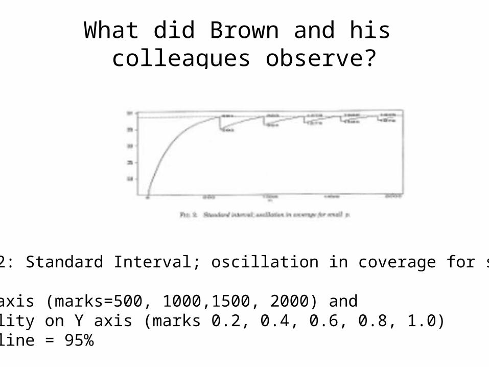
Figure 2: Standard Interval; oscillation in coverage for small p

n on X axis (marks=500, 1000,1500, 2000) and probability on Y axis (marks 0.2, 0.4, 0.6, 0.8, 1.0)dashed line = 95%

Introductory Stats Texts

Usually present the Wald 95% CI for the one-samplecase using the central limit theorem so that as n approaches infinity, coverage approaches 95%

Brown and his colleagues demonstrated that this doesnot hold.

Nonnegligible Oscillation

There exist some “lucky” pairs (p,n) such that theactual coverage probability is very close to or larger than 1-α.

On the other hand, there are also unlucky pairs (p,n)such that coverage is much smaller than 1-α.

Furthermore, drastic changes in coverage occur in nearby p for fixed n, and in nearby n for fixed p.

Where does the Coverage Error come from?

The authors state that the coverage probabilityerrors comes from two sources;

discretenessskewness

Of the underlying binomial distribution.

Recommended Intervals: Wilson

Inverts the WALD large sample test but uses the nullstandard error instead of the estimated standard error:

Recommended Intervals: Agresti-Coull

Replace with

and with

Agresti-Coull intervals are never shorter than theWilson intervals.

Recommended Intervals: Jeffreys Equal Tailed

Bayesian interval basedon a non-informative conjugateBeta prior Beta( ½, ½) with density function

The 100(1-α)% equal-tailed Jeffreys equal-tailed interval is defined as

where and otherwise

α/2 posterior probability omitted from each tail

Recommended Intervals: Jeffreys Equal Tailed

Jeffreys Equal-tailed CI is always contained in the Clopper-Pearson CI and can be regarded as a continuity corrected version of the Clopper-Pearson Interval

Recommended Intervals: Coverage

• The standard CI performed poorly• The Agresti-Coull CI was slightly conservative• The Wilson and Jeffreys Equal-Tailed CIs average coverage performed excellently • Close to p=0,1 Wilson, Jeffreys Equal-Tailed and the standard CI did not perform so good. Agresti-Coull CI was somewhat conservative. A modification to the Wilson CI produced conservative coverage.

Recommended Intervals: Length

• The standard CI was shorter in length when p close to 0 or 1• Wilson and Jeffreys ET CI lengths were very similar• Agresti-Coull was slightly longer in length when n was small

Others Intervals Considered

• Clopper-Pearson• Arcsine• Logit• Mid-p Clopper Pearson• Jeffreys Bayesian HPD• The likelihood Ratio Interval

What do the Authors Recommend?

• Wilson or equal-tailed Jeffreys for small n (n ≤ 40)• For larger n, the Wilson, Jeffreys ET and Agresti-Coull are all comparable• They do not recommend use of the standard interval under any circumstances when computing the CI for an one-sample Binomial proportion.

Two-sample Binomial Proportions

The oscillation observed in the one sample caseis not a serious problem in calculating CIs for the two-sample difference in binomial proportions.

For a further discussion of this topic, refer to

Lawrence Brown & Xuefeng Li“Confidence intervals for two sample binomialDistribution”, Journal of Statistical Planning & Inference(2005) 359-375

References

• Interval Estimation for a Binomial Proportion. Lawrence D. Brown, T. Tony Cai and Anirban Dasgupta. Statistical Science 2001; Vol. 2, 101-133

• Confidence Intervals for two Sample Binomial Distribution. Lawrence Brown and Xuefeng Li. Journal of Statistical Planning and Inference 2005; 130, 359-375

Additional Slide 1Coverage probability for n=50

X axis represents p and ranges from 0 to 1. Y axis represents coverage prob and ranges from 0.86 to 1.00

Clockwise starting from top left: Standard interval, Wilson, Jeffreys Equal-Tailed and Agresti-Coull

Additional Slide 2Coverage probability for n=50

Clockwise starting from top left: Arcsine, Clopper-Pearson, Logit and Jeffreys Prior HPD

X axis represents p and ranges from 0 to 1. Y axis represents coverage prob and ranges from 0.86 to 1.00