Do Value Investors Add Value? - csinvesting.orgcsinvesting.org/.../2013/02/Do_Value_Investors_Add_Valueshort.pdfare Reyer Barel and Saj Karsan (1999-2006), Dalton Baretto, Scott Gryba,

1

Do Value Investors Add Value?

George Athanassakos* Ben Graham Chair in Value Investing

Richard Ivey School of Business The University of Western Ontario London, Ontario, Canada N6A 3K7

[email protected] www.bengrahaminvesting.ca

Version 09.20-2

May 2010

Please do not Quote without Permission

Comments Welcome

* This paper represents an extension of a pilot study carried out at the Richard Ivey School of Business in 2008 by George Athanassakos, Reyer Barel and Saj Karsan entitled “Searching for and Finding Value: Canadian Evidence 1999-2006”. The pilot project and its extension have been funded by an Ivey Research Grant and would not have been possible without the hard work and commitment of a group of students who worked diligently on company valuations. The students and the time periods they covered are Reyer Barel and Saj Karsan (1999-2006), Dalton Baretto, Scott Gryba, Ali Sabur and Carter Yu (1985-1998) and Scott Gryba, Ali Sabur and Carter Yu (2007-2009). Many thanks also go to Carly Vanderheyden for excellent assistance.

mailto:[email protected]

http://www.bengrahaminvesting.ca/

2


A B S T R A C T

The purpose of this paper is first to examine whether a value premium exists following a mechanical screening process (i.e., the search process) in the Canadian markets between two distinctly different periods, 1985-1999 and 1999-2007, and second whether value investors add value in the stock selection process by being able to find truly undervalued stocks from the universe of the possibly undervalued stocks identified from the search process. We find that a strong and pervasive value premium exists in Canada over our sample periods that persists in bull and bear markets and during recessions/recoveries. Value stocks, on average, beat growth stocks even when using the very mechanical screening of the search process. Furthermore, this paper demonstrates that value investors do add value, in the sense that their process of selecting truly undervalued stocks, via in-depth security valuation of the possibly undervalued stocks and arriving at their investment decision using the concept of “margin of safety”, produces positive excess returns over and above the naive approach of simply selecting low P/E - P/BV ratio stocks. The paper was extended to the years of the “great recession” (2008-2009) and despite the fact that over this extended period we had a severe recession and bear market, on average, the sophisticated portfolio still beat the naïve value portfolio, consistent with earlier evidence.

3


1. Introduction

A large body of academic research has shown that value stocks (i.e., low price-to-earnings (P/E) or price-to-book value (P/BV) stocks) tend to have higher average returns than growth stocks (i.e., high P/E or high P/BV stocks). Basu (1977) was the first to confirm the existence of a value premium, namely, that value stocks outperform growth stocks. More recently, Chan, Hamao and Lakonishok (1991), Fama and French (1992, 1993, 1996), Lakonishok, Shleifer and Vishny (1994), Chan and Lakonishok (2004) and Athanassakos (2009, 2011) have found evidence consistent with a positive value premium in markets around the globe using not only P/E based classifications of stocks into value and growth, but also other search criteria which value investors have traditionally used to divide stocks into value and growth, such as P/BV and dividend yield.

While academic papers, such as the ones referred to above, have claimed to examine value and growth strategies and their performance, such claim is only partly correct. The problem with the academic classification of stocks into value and growth is that such stock selection approach is only part of what value investors do! Value investors use the above mentioned screening process, namely screening for the low P/E or low P/BV stocks, to identify possibly undervalued stocks. But this is not all. This is the first step they follow in stock selection. Once the possibly undervalued stocks are screened out, value investors then proceed to the second step of their analysis which is to identify the stocks that are truly undervalued by valuing individually each stock and arriving at their investment decision using the concept of the “margin of safety”.

Unfortunately, academics do not and cannot know which stocks value investors eventually choose to invest in and so they only look at the first step of value investors’ stock selection process. After all, academics know that it is from this group of low P/E or low P/BV stocks that value investors tend to select stocks to invest in. Consequently, academics tend to call the low P/E (or P/BV) stocks value stocks and the high P/E (or P/BV) stocks growth stocks, as this latter group of stocks is not the group of stocks from which value investors typically tend to select stocks to invest in. The first step of stock selection, and the one the academics have examined, is a naïve process and entirely mechanical. Anyone can run such a stock screening selection process to identify possibly undervalued stocks. The value that value investors add, however, is with regards to their second step of stock selection, namely, valuing each stock individually and using the concept of “margin of safety” in order to identify the truly undervalued stocks. And it is this step in particular that previous academic research has not examined.

Using Canadian data for two distinctly different sub-periods 1985-1999 and 1999-2007, this paper has two objectives.1 The first is to confirm that a value premium exists in our sample of stocks using a search process (i.e., the first step of stock selection) that consists of cross-sorting stocks by both

1 These periods were chosen and kept separate for the following reasons: The first sub-period (1985-1999) was

characterized by a classic bull market with steadily rising stock prices, while the second sub-period (1999-2007) was a most challenging period for the stock market – with the exception of the materials and oil sectors, the stock market overall remained mostly flat over this sub-period which also included the burst of the stock market bubble. The paper was also subsequently extended to cover the years of the “great recession” (2008-2009).

4

P/E and P/BV ratios. Our hypothesis here is that we expect (potentially) value stocks (i.e., low P/E - low P/BV) to beat growth stocks (i.e., high P/E - high P/BV).2 The second is to examine whether the second step of valuation and stock selection that value investors follow adds any value. In this regard, our hypothesis is that if value investors really add any value, stocks found to be truly undervalued (i.e., the truly value stocks), on average, beat stocks selected naïvely via the first step of stock selection (i.e., the potentially value stocks).3 The key objective of this paper, and the paper’s main contribution, is with regards to testing the second hypothesis and answering the following related question: Do value investors add value? Previous academic research has said nothing about the value of value investors; this paper will.

We find that a strong and pervasive value premium exists in Canada over our sample sub-periods that persist in bull and bear markets and during recessions/recoveries. Furthermore, this paper demonstrates that value investors do add value, in the sense that their process of selecting truly undervalued stocks, via in-depth security valuation of the possibly undervalued stocks and arriving at their investment decision using the concept of “margin of safety”, produces positive excess returns over and above a naive approach of simply selecting low P/E - P/BV ratio stocks.

The rest of the paper is structured as follows. Section 2 discusses the data and methodology. Section 3 presents the empirical findings, while section 4 concludes the paper.

2. Data and Methodology

This paper uses data from COMPUSTAT from which earnings per share (E), book value per share (BV), shares outstanding, stock prices, and dividends paid are obtained, and from which trailing price to earnings (P/E) and price to book value (P/BV) ratios and market cap are derived. For the trailing P/E and P/BV ratios, the price (P) is as of the end of April of year (t) and E and BV are, respectively, the December (t-1) fully diluted annual earnings per share and book value per share for companies with fiscal year end December (t-1), as reported in COMPUSTAT. Market cap is derived by multiplying price per share times shares outstanding at the end of April of year t. Annual total stock returns for the second sub-period are calculated as the price change plus the dividend from April of year t to April of year t+1 over the price in April of year t, using COMPUSTAT. For the first sub-period, due to data unavailability, annual total returns were calculated as above, but data for the calculation were obtained from the Canadian Financial Markets Research Center (CFMRC) data base.

Our sample includes all December fiscal year end non-financial services companies that trade on the Toronto Stock Exchange (TSX).4 Based on this, we started with COMPUSTAT’s industrial 4443 year-firm observations (data) belonging to 1263 companies for the period 1985-1999, and 4503 year-firm observations (data) belonging to 1081 companies for the period 1999-2007. We carried out a number of

2 Previous academic evidence supports this hypothesis (See Basu (1977), Chan, Hamao and Lakonishok (1991), Fama

and French (1992, 1993, 1996), Lakonishok, Shleifer and Vishny (1994), Chan and Lakonishok (2004) and Athanassakos (2009, 2010)). 3 The performance of legendary value investors, such as Mr. Warren Buffett and Mr. Walter Schloss, over long time

periods supports this hypothesis. Under Mr. Buffett, Berkshire Hathaway has averaged a 25%+ annual return to its shareholders for the last 25 years, while employing large amounts of capital and minimal debt. Mr. Schloss and his son Edwin, over the period 1956 to 2000, provided investors a compounded return of 15.3% compared with the S&P 500’s annual return on 11.5% (See http://www.bengrahaminvesting.ca/Teaching_Applications/Guest_Speakers/2008_speakers.htm). 4 We exclude financial services companies, such as banks and insurance companies, since the high leverage normally

employed by these companies does not have the same meaning as for non-financial companies for which high leverage indicates financial distress.

5

screenings to the data. Companies are not income trusts. Companies are required to have return data available for the year following the determination of P/E and P/BV ratios unless a company was acquired in which case the stock return for the remaining annual period was assumed to be the Canadian t-bill 6 month rate obtained from the Bank of Canada database. To prevent problems arising from including negative or extremely positive P/E and P/BV ratio firms, and eliminate likely data errors (See La Porta, Lakonishok, Shleifer and Vishny (1997), Griffin and Lemmon (2002) and Cohen, Polk and Vuolteenaho (2003)), we have excluded negative P/E and P/BV ratios, as well as P/E ratios in excess of 150 and P/BV in excess of 20. Firms had to have both P/E and P/BV ratios within the aforementioned boundaries to be included in the sample. Finally, to be included in our sample a stock had to have a price over $1.5,6

Our data, which are adjusted for stock splits and stock dividends, are for each year over two distinctly different sub-periods, 1985-1999 and 1999-2007.7 After all aforementioned screenings, we end up with 2139, in 1985-1999, and 1301, in 1999-2007, cross sectional-time series (firm-year) observations belonging to a cumulative number of 406 and 377 unique companies, respectively over the two sample sub-periods. The tables below report the total number of observations (companies examined) per year for each sub-period.

Sub-period 1985-1999

Year Number of Observations

1985 133

1986 142

1987 139

1988 168

1989 147

1990 135

1991 126

1992 98

1993 116

1994 164

1995 222

1996 174

1997 178

1998 197

At the end of April of every year (t), starting either in 1985 or in 1999, firms are ranked based on

trailing P/E ratios from low to high and the ranked firms are divided into four groups of equal size. Each P/E based quartile is then subdivided into four quartiles based on P/BV ratios from low to high. This

5 Since our sample only includes firms with fiscal year end December of year (t-1), all firms have released their annual

reports needed for the valuations and information for earnings per share and book value per share by April of year (t). 6 For sub-period 1985-1999, the no income trust screen eliminated 182 observations, price over $1 39 observations,

the P/E restrictions 722 observations and the P/BV restrictions 108 observations. In addition, 407 and further 846 observations were eliminated as there were no price and EPS data, respectively available in COMPUSTAT. For sub-period 1999-2007, the no income trust screen eliminated 971 observations, price over $1 622 observations, the P/E restrictions 563 observations and the P/BV restrictions 15 observations. In addition, 811 and further 220 observations were eliminated as there were no price and EPS data, respectively available in COMPUSTAT. 7 See footnote #1 for the reasons these periods were kept separate.


Year Number of

Observations

1999 162

2000 175

2001 177

2002 148

2003 144

2004 150

2005 167 2006 178

6

process is repeated for each year of our sample. Membership in a quartile changes each year as multiples change from year to year. Inclusion in a quartile depends on a stock’s multiple in relation to other stocks’ multiples. Because P/E and P/BV ratios change over time, an arbitrary measure across time for all stocks in our sample would be inappropriate. The range of P/E – P/BV ratios per year for the low P/E – low P/BV basket (Q1) and the high P/E – high P/BV basket (Q16), per sub-period, are reported in the tables below.

In the first sub-period, we end up with 140 observations in both the low and high P/E - low P/BV

baskets (Q1 and Q16). In the second sub-period, we end up with 81 observations in the low P/E - low P/BV basket (Q1) and 85 observations in the high P/E - high P/BV basket (Q16).8

8 The reason for this discrepancy in the latter sub-period is the following. Unlike Q16, we actually carry out valuations

on Q1 stocks and while a few stocks in the low P/E - low P/BV basket did not possess the ticker suffix used for filtering income trusts, namely .U, upon closer inspection during valuation of Q1 stocks, we found that some stocks were actually income trusts and, thus, were subsequently eliminated. For this reason, in some years, we have fewer stocks in Q1 than Q16.


Q1 (Value) Q16 (Growth)

Year P/E P/BV P/E P/BV

1999 Min 2.38 0.35 25.00 2.41 1999 Max 9.72 0.72 83.72 17.64 2000 Min 0.42 0.39 29.12 3.87 2000 Max 7.23 0.67 144.00 11.48 2001 Min 2.65 0.27 21.46 3.28 2001 Max 8.19 0.78 140.00 8.52 2002 Min 3.45 0.33 27.17 3.76 2002 Max 8.72 0.78 133.33 6.41 2003 Min 3.26 0.47 23.91 2.85 2003 Max 9.82 0.72 85.00 5.23 2004 Min 5.05 0.54 28.64 3.31 2004 Max 10.77 1.09 135.00 7.19 2005 Min 4.05 0.73 30.95 4.94 2005 Max 11.30 1.03 135.00 13.34 2006 Min 2.55 0.58 29.80 4.57 2006 Max 12.82 1.27 86.11 18.61



Year P/E P/BV P/E P/BV

1985 Min 3.15 0.48 17.73 2.87

1985 Max 8.92 0.74 52.28 8.00

1986 Min 3.87 0.40 24.22 4.46

1986 Max 10.25 0.86 48.65 17.42

1987 Min 1.61 0.23 29.18 4.23

1987 Max 13.93 1.23 101.48 30.00

1988 Min 1.18 0.11 22.52 2.87

1988 Max 8.28 0.90 49.50 10.51

1989 Min 7.30 0.43 18.68 2.33

1989 Max 8.88 1.01 55.09 12.70

1990 Min 3.93 0.14 18.71 2.29

1990 Max 6.84 0.79 41.60 6.46

1991 Min 2.41 0.14 26.14 1.78

1991 Max 9.49 0.82 103.13 8.47

1992 Min 7.49 0.42 35.94 2.83

1992 Max 11.88 1.09 146.15 4.55

1993 Min 5.68 0.70 53.33 2.99

1993 Max 13.01 1.12 93.75 13.54

1994 Min 2.28 0.41 37.09 4.01

1994 Max 10.95 1.15 130.00 47.77

1995 Min 2.76 0.26 25.51 2.79

1995 Max 10.18 0.91 105.00 6.91

1996 Min 1.41 0.45 33.27 3.91

1996 Max 9.13 0.78 137.50 12.15

1997 Min 4.40 0.70 26.41 3.18

1997 Max 12.10 1.04 89.63 5.87

1998 Min 0.66 0.56 32.45 4.04

1998 Max 15.45 1.02 129.41 20.51

7

For each stock within each portfolio, returns are obtained for the following year (starting in May

1, 1985 or 1999 and ending April 30, 1999 or 2007, respectively in each sub-period) and equally weighted mean (and median) returns for each portfolio (basket) are derived (See Fama and French (1992), Lakonishok, Shleifer and Vishny (1994) and La Porta, Lakonishok, Shleifer and Vishny (1997)). Basket-1 (Q1) is the lowest P/E - lowest P/BV ratio portfolio or the value stocks, while Basket-16 (Q16) is the highest P/E - highest P/BV ratio portfolio or the growth stocks.9 For each sub-period, the number of observations for each basket per year is reported in the tables below. The 140 overall observations for the first sub-period belong to 78 unique companies for Q1 and 75 unique companies for Q16. The 81 overall observations in Q1 and 85 observations in Q16 for sub-period 1999-2007 corresponded to 48 and 59 unique companies, respectively.

9 The P/E and P/BV sorting requirement was made in order to reduce the number of stocks we had to actually evaluate

due to the labor intensity of the project.



Year Number of

observations Number of

observations

1985 8 8

1986 9 9

1987 9 9

1988 11 11

1989 10 10

1990 9 9

1991 8 8

1992 7 7

1993 8 8

1994 11 11

1995 14 14

1996 11 11

1997 12 12

1998 13 13



Year Number of

observations Number of

observations

1999 10 10

2000 10 11

2001 11 12

2002 8 9

2003 9 10

2004 10 10

2005 11 11

2006 12 12

Total 81 85

8

A time series of non-overlapping annual returns are obtained for each stock within the Q1 and Q16 portfolios (and for each portfolio) from May 1, 1985 (1999) to April 30, 1999 (2007). Summary statistics of variables of interest (i.e., value and growth stock returns, value premium, market cap) for the various stocks and portfolios are calculated and univariate analysis ensues that looks at value and growth stock performance and the value premium. If a stock stopped trading due to an acquisition, then the remaining of the year returns for this stock were estimated as being the Canadian 6-month t-bill rate of return obtained from the Bank of Canada database.10

As soon as a value premium is established, we then go on to determine whether the second step

of the value investing process, namely, valuing each stock and determining whether it is truly undervalued to buy, will beat the naïvely determined value stocks, namely, the first step of the value investing process.

To determine the truly undervalued stocks, the naively chosen stocks from Q1 were individually valued. The annual reports of the companies in question were obtained from Sedar.com. The objective here was to see if investing in the truly undervalued stocks, using a valuation approach employed by value investors, will lead to returns higher than those of the naively chosen Q1 stocks.

For each stock in Q1, two valuations were carried out. First, the net replacement value of each company’s assets (called Net Asset Value) was estimated using an approach similar to the one described in Greenwald etc. (2001). Second, a Free cash Flow (FCF) based valuation for each company was produced (called Earnings Power Value), by normalizing FCFs and discounting them to infinity using a perpetuity formula. The discount rate was the weighted average costs of capital (WACC), with the cost of equity obtained from the bond plus risk premium approach described in Athanassakos (1998), and the cost of debt obtained from the company’s rating and the YTM of similarly rated companies obtained from Canadian Bond Rating Service and Scotia Capital Markets (1985-1999) and Moodys and Bloomberg (1999-2007). The weights in the WACC formula were the company’s target capital structure weights.

Value investors believe that in the long run, in a free entry market, the return on invested capital (ROIC) will be equal to WACC, and so for the majority of companies the Discounted Cash Flow (DCF) model becomes one of perpetuity. However, if a company has a sustainable competitive advantage, a (real) growth assumption is incorporated in the DCF model and the value with growth (Vg) is derived.

Consequently, for each company two values were derived. One was the Net Asset Value (NAV) and the other the Earnings Power Value (EPV). Where exactly the company’s intrinsic value lied depended on strategic analysis and the probabilities of possible outcomes. If the NAV exceeded the EPV, a catalyst was assumed depending on the probability of a takeover or the probability of management change given public information available in the financial press. In this case, the company’s intrinsic value was between NAV and EPV. Whether the intrinsic value was closer to NAV than EPV depended on how high or low the probability of the aforementioned changes was, respectively. If EPV was above NAV, then an analysis of the company’s competitive environment was made to determine whether the company had a sustainable competitive advantage. If that was the case, then the company’s intrinsic

10

For Q1, there were 1 stock in 1986, 1993, 1996, 1997, and 2002, and 2 stocks in 2000 that stopped trading within a given year. For Q16, there was 1 stock in 1986, 1987, 1997, 2000, 2001 and 2002 that stopped trading within a given year. Combined in Q1 and Q16, we had overall 7 companies in 1985-1999 and 6 companies in 1999-2007 for which we had to use the 6 month t-bill assumption. The stocks contained in Q1 and Q16, as well as the stocks that stopped trading within a year and a t-bill assumption had to be made are available from the author upon request.

9

value was its EPV; if not, the company’s intrinsic value was between EPV and NAV. How close to EPV or NAV the intrinsic value was depended on how strong we felt, given available information and our strategic analysis of the industry and company, the probability of sustainability of competitive advantage was. The lower this probability, the closer to NAV the intrinsic value was and vice versa. If a (real) growth assumption was necessary, then the value with growth was estimated (Vg) which for obvious reasons exceeded EPV (the no growth valuation to perpetuity). In this case, the company’s intrinsic value was Vg. We found 87 cases in the first sub-period and 54 cases in the second sub-period, in which NAV was above EPV, 2 and 18 cases, respectively for which EPV was above NAV and no case and only 1 case, respectively for which a growth assumption was necessary, that is, when Vg was higher than EPV.11 Once, the intrinsic value was estimated, the entry price was calculated as 2/3 of the intrinsic value. This allowed for 1/3 margin of safety. The entry price in the growth case was the lower of EPV or 2/3 of Vg.

If a stock’s current price was below the entry price, a decision was made to invest in this stock; the stock was truly undervalued. Otherwise, a decision was made not to invest in the stock in the following 12 month period. At the end of each 12-month period, stocks were liquidated and annual returns were calculated for this period. At the beginning of the next 12-month period, new intrinsic values and entry prices were re-estimated. Stocks whose current price was below their re-estimated entry price were invested in the new sophisticated portfolio for the following 12 months, and the process continued for every subsequent 12-month period. That is, at the beginning of each 12-month period, every stock in the sophisticated portfolio needed to have met the condition of having a price less than its entry price to justify its position in the following year’s sophisticated portfolio. While this portfolio rebalancing may not be entirely true for all value investors many of whom may still be invested in the stock as long as it hasn’t reached its intrinsic value, the fact that a stock moved up over the previous year and was now above its new entry price may mean that much of the upside on the stock has been realized and better investment opportunities may exist in other stocks with price less than entry price that were worth investing in with higher upside. Besides, our objective was to compare the returns of the sophisticated portfolio to those of the naïve Q1 portfolio and, to do this accurately and consistently, we needed to derive annual total returns for both portfolios. Since the assumption of once a year rebalancing applied to Q1, the same assumption was also made for the sophisticated portfolio. The final number of stocks per year in the invested “sophisticated” portfolio (Q1S) is shown below. The total number of stocks purchased in the sophisticated portfolio corresponds to 44 companies (30 unique companies) in the first sub-period and 33 companies (24 unique companies) in the second sub-period. That is, a few companies were repeat members of the sophisticated portfolio as, year after year, they met the price less than entry price condition.

11

In the first sub-period, the valuation team found a number of companies that were outside their “circle of competence” to value reliably. These companies were (26) resource companies (eliminated due to uncertain real options), (6) private equity firms or holding companies (eliminated due to uncertain value of investments or holdings) and (12) companies of high business and financial risk (due to extreme financial distress situations). In addition, five companies had no data available and 2 companies were recent IPOs for which no historical data were available and they were thus eliminated from the valuation step. The exclusion of such companies also helped reduce the number of companies that had to be valued and made the project more manageable. As a result, 89 companies were actually valued and not 140 as originally indicated for sub-period 1985-1999. In the second sub-period, where there were fewer companies to be valued, at the valuation step, the valuation team eliminated six companies that had high business and financial risk and two companies for which annual reports were not available. No other companies were eliminated in this sub-period as the valuation team felt that the remaining companies were within their “circle of competence” and could be reasonably valued. As a result, 73 companies were actually valued and not 81 as originally indicated for sub-period 1999-2007.

10


Year

# of Stocks in Sophisticated Portfolio

1985 3

1986 3

1987 2

1988 2

1989 3

1990 3

1991 1

1992 1

1993 3

1994 3

1995 4

1996 5

1997 7

1998 4


Year

# of Stocks in Sophisticated Portfolio

1999 4

2000 6

2001 5

2002 4

2003 4

2004 2

2005 4

2006 4

To our knowledge, this is the first study to examine both steps of the value investing decision making approach and explore whether value investors add value to the strictly mechanical search process.

3. Empirical Results

3.1. Step 1: The search Process - Is There a Value Premium?

Table 1 reports the mean and median annual returns of P/E - P/BV sorted value (Q1) and growth (Q16) portfolios and the value premium (Q1 minus Q16) per year and overall. Table 1 also reports the variance of returns of the value and growth portfolios and their Sharpe ratio performance metrics for the two sub-periods examined.

It is quite apparent from this Table that a value premium exists and it is quite impressive for its size and consistency, particularly for the 1999-2007 sub-period. The mean value premium per year in Table 1 is mostly positive. In the years when the value premium is negative, the size of the value premium is relatively small, when compared with the years when the value premium is positive. All median annual value premiums are positive. For 1985-1999, the mean (median) annual value premium (Q1-Q16) is 2.4% (3.7%). For 1999-2007, the mean (median) annual value premium is 16.60% (16.00%). For comparative purposes, using only P/E sorting, Athanassakos (2009) finds that the mean value premium in Canada for the period 1985-2005 is 6.30%, whereas Athanassakos (2011), using again P/E sorting, finds that the mean value premium in the US is 6.24%, 11.40% and 6.00% for AMEX, NASDAQ and NYSE stocks, respectively for the period 1986-2006.

Table 1 also allows us a glimpse into the behavior of the value premium during recessions and/or bear markets. For example, www.thedowtheory.com/bear&recessions.htm reports years 2000

http://www.thedowtheory.com/bear&recessions.htm

11

and 2002 as bear market years and years 1991 and 2001 as recessionary years. With the exception of the mean value premium in 1991 which is negative, Table 1 shows that irrespective of the state of the world, the value strategy normally beats the growth strategy. As far as the mean returns are concerned, Table 1, Panel A shows that in 1991, a recessionary year, the growth strategy beats the value strategy by 6.3%. Table 1, Panel B, however, shows that in the bear market years value and growth portfolios experience about the same return, whereas in 2001, the year of recession, value clearly beats growth. As far as the median returns are concerned, Table 1, Panel A shows that the value premium is positive in 1991, the recessionary year. In Table 1, Panel B all value premiums are positive in both bear markets years (2000 and 2002) and recessionary year (2001). It can also be easily inferred from Table 1 that value premiums in adverse states of the world are mostly comparable to the value premiums in favorable states of the world over our two sample periods, particularly the 1999-2007 sub-period. These findings are consistent with Athanassakos (2009, 2011) and Kwag and Lee (2006) who, similar to our findings, show that value stocks in Canada and the US, on average, outperform growth stocks throughout the business cycle.

How does the variance and firm-size of the value stocks compare to those of the growth stocks? Table 1 reports the variance of the annual returns of the value and growth portfolios, while Table 2 reports market cap of the value and growth portfolios per year over our two sub-periods. These tables show that value stocks tend to be smaller than growth stocks and that while the value portfolio has higher annual variance of returns than the growth portfolio in the second sub-period, the opposite is the case in the first sub-period. The smaller size of Q1 vs. Q16 may imply that the outperformance of value over growth stocks is driven by risk, as normally one would expect smaller stocks to have higher risk than larger stocks. However, if risk drove the findings, one would expect to find (a) consistently higher variance in the returns of value vs. growth stocks and (b) that the higher risk of value stocks is manifested more vividly during adverse states of the world (such as recessions and bear markets) at which time growth would beat value strategies. As this is not the case, one cannot attribute the return differences between value and growth stocks to possible higher risk of value stocks.12

Furthermore, Table 1 shows that the Sharpe ratio of value stocks (0.24 in 1985-1999; and 0.83 in 1999-2007) exceeds the Sharpe ratio of growth stocks (0.14 in 1985-1999; and 0.75 in 1999-2007) indicating that value stocks have had a better risk adjusted performance than growth stocks over our sample sub-periods. The p-value of the difference between the Sharpe ratios of these two portfolios, calculated based on a test of significance discussed in Jobson and Korkie (1981), is 0.09 in 1985-1999 and 0.03 in 1999-2007.

Could it be that the value premium is driven only by a few value stocks with very large positive returns? Table 3 reports the percentage of stocks with positive and the percentage of stocks with negative returns for the value and growth portfolios for every year over our sample sub-periods. In the first sub-period, both value and growth stocks experience more positive than negative returns in 9 out of the 14 years. In the second sub-period, in every year, more stocks in the value portfolio have positive returns than negative. This is true only in 4 out of the 8 years for the growth portfolio. Consequently, the value premium is pervasive and not the result of a few outliers.

12 The risk issue will also be addressed in the following section, where risk is incorporated in the valuation exercise,

intrinsic value, entry price and final investment decision making.

12

3.2. Step 2: Valuation – Is Any Value Added?

Now that we established that there is a value premium over our sample sub-periods which is consistent with previous academic research, the question is: can a value investor with his/her ability to value stocks, using value investing principles, do better than an approach that naively picks a basket of stocks with the lowest P/E – P/BV ratio combination?

All stocks that were previously sorted in the value basket (Q1) are now individually valued in a very time consuming and laborious way. First, the intrinsic value of a stock is estimated as discussed earlier and then the entry price is calculated as intrinsic value less 1/3 of the intrinsic value - the margin of safety. If a stock’s current price is below its entry price, a decision is made to buy this particular stock. If not, a decision is made not to purchase the stock. We refer to the portfolio with the stocks in which we choose to invest as the “sophisticated portfolio” (Q1S), whereas the value portfolio Q1 is referred to as the “naïve portfolio”. The annual and overall mean and median returns of the sophisticated portfolio and its excess returns from the naïve value Q1 portfolio are reported in Table 4.13

The sophisticated portfolio (Q1S) beats the naïve value Q1 portfolio both in mean and median returns. The mean (median) outperformance in sub-period 1985-1999 is 1.10% (3.30%), while in sub-period 1999-2007 is 13.20% (3.80%). Table 4 also shows that the sophisticated portfolio beats the naïve one in both bear market years and the recessionary market years. Irrespective of the state of the world, both the mean and median returns of the sophisticated portfolio exceed those for the naive portfolio. Moreover, it can be easily inferred from Table 4 that the sophisticated portfolio outperforms the naïve portfolio by more in adverse states of the world than in favorable states of the world. Finally, Table 5 reports that, in general, the percentage of positive returns in the sophisticated portfolio is higher than the percentage of positive returns in the naïve portfolio.

Table 4 also shows that the variance of the sophisticated portfolio is somewhat higher than the variance of the naïve one, while Table 6 shows that the market cap of these two portfolios is about the same. The risk adjusted returns of the sophisticated portfolio exceed those of the “naive portfolio” as exemplified by the higher Sharpe ratio of the sophisticated portfolio than the naïve one (See Table 4). The Sharpe ratio for the sophisticated and naïve portfolios is 0.30 vs. 0.24 in 1985-1999, and 1.07 vs. 0.83, in 1999-2007, respectively.14 The p-value of the difference between the Sharpe ratios of these two portfolios, again calculated based on a test of significance discussed in Jobson and Korkie (1981), is 0.15 in 1985-1999 and 0.01 in 1999-2007.15

Moreover, the valuation exercise described above and the eventual decision to buy a stock in the sophisticated portfolio accounts for risk and makes the final stock selection less risky in the sense of reducing the possibility of loss of capital.16 Preserving capital is of paramount importance in the

13

The kind of reports we produced for each stock in portfolio Q1, as well as the actual stocks we chose to purchase and include in the sophisticated portfolio (Q1S) per sub-period after painstaking valuations are available from the author upon request. 14

It is possible that the exclusion of the companies indicated in footnote #9 from the second step of the value investing process may have impacted the strength of the findings in the first sub-period as there may have been many truly undervalued stocks among the excluded companies. 15

It should be noted that this test has low power in the sense that is it is difficult to find statistical significance even if the true difference in Sharpe ratios is not zero. 16

The issue of whether risk or behavioral factors drive the value premium has arisen because academics deal only with the first step of the value investing process. Not knowing what stocks value investors tend to buy, academics resort to

13

investment decision process of value investors. The margin of safely taken off the intrinsic value to arrive at the entry price ensures downside protection that goes beyond diversification without sacrificing the returns of the chosen stocks. In addition, Q1 and Q1S are both from the same basket of stocks and have the same market cap as shown in Table 6. And the fact that the sophisticated portfolio beats the naïve one by more in adverse than favorable states of the world further supports the argument that the risk of the sophisticated portfolio is not higher than that of the naïve portfolio. Hence, risk does not seem to drive the outperformance of the stocks that value investors choose to eventually invest in (i.e., the truly undervalued stocks), which is the key contribution of this paper.

Finally, not only does the sophisticated portfolio beats the naïve portfolio Q1, but Q1 significantly beats Q16, making the sophisticated portfolio outperform Q16 by a substantial amount, which is too large to be explained by possible risk differences. As a result, value investors proceeding to the second step in the stock selection process do add value.17

3.3. How About 2007-2009?

This study had started well before the credit crisis of 2008-2009 engulfed the world economies and markets. It ended right at the time the credit crisis hit.

As data have now become available for 2008 and 2009, and as readers will be interested in knowing how the value investing approach worked over this period of crisis, we decided to extend this paper to also include the credit crisis period.

The methodology and process are the same as described earlier. Following same screenings as before, we end up with 223 observations in 2007 and 183 observations in 2008. We then form Q1 (the value portfolio) and Q16 (the growth portfolio) for 2007 and 2008 with the following ranges for P/E and P/BV: Q1-2007 (min P/E: 3.60, max P/E: 11.92; min P/BV: 0.71, max P/BV: 1.23); Q1-2008 (min P/E: 3.80, max P/E: 11.14; min P/BV: 0.62, max P/BV: 1.10); Q16-2007 (min P/E: 33.46, max P/E: 144.14; min P/BV: 5.38, max P/BV: 10.15); Q16-2008 (min P/E: 31.04, max P/E: 112.47; min P/BV: 4.36, max P/BV: 15.93). There were 14 observations in 2007 and 12 observations in 2008 for Q1 and Q16. We only found 2 truly undervalued stocks in 2007 and only 1 truly undervalued stock in 2008, and these stocks were included in the sophisticated portfolio.

Table 7 shows the mean and median annual returns for Q1 and Q16, while Table 8 shows the mean and median annual returns for Q1S (the “sophisticated” (value) portfolio) and Q1 (the ”naïve” (value) portfolio) for the period May 1, 2007 to April 30, 2009. In addition, this time, the Tables also show the returns for Q1, Q16 and Q1S from May 1, 2008 to September 30, 2009 (referred to as 2008 extended). These Tables’ extended period returns represent seventeen month returns for Q1, Q16 and Q1S portfolios, as if the stock selections and compositions for value, growth and sophisticated portfolios had not changed from May to September 2009.

arguments about risk to justify the value premium (See Fama and French (1992, 1993, 1996)). However, if one knows the intrinsic value of a stock and its entry price (which accounts for the margin of safety), and, hence, what stocks value investors would buy, as per second step of the value investing process, then he/she should know the risk of the portfolio/stocks. In the valuation process, risk is adjusted through the risk premium in the discount factor and in the final selection process risk is controlled for via the margin of safety. 17

Our sophisticated portfolio is quite concentrated. However, the margin of safety acts as a way to protect capital which is distinct from, and in many respects consistent with, diversification. Moreover, the superior performance of the sophisticated portfolio is consistent with Kacperczyk, et al. (2007) who find that all concentrated funds in their study did well, but the more concentrated did the best.

14

We see that over the two years of the “great recession”, the mean and median returns for the growth portfolio (Q16) exceed those for the value portfolio (Q1) by a significant amount for both the normal and extended period. On the other hand, the sophisticated portfolio (Q1S) under-performed the naïve portfolio (Q1) in 2007, but significantly outperformed it in 2008 for both the normal and extended 2008 period. In fact, in 2008, the sophisticated portfolio outperformed both the naive value and the growth portfolio. On average, over the two year period, the sophisticated portfolio beat the naïve portfolio and the growth portfolio. Moreover, the sophisticated portfolio beat the naive during the recession and the bear market period of May 1, 2008 to April 30, 2009. These findings are consistent with those reported earlier for 1985-2007.

4. Conclusions

Value investors wish to buy stocks at a discount to intrinsic value. To find the heavily discounted stocks, value investors follow a two step process. First they search for possibly undervalued stocks, using screening metrics, such as P/E and/or P/BV ratios. Second, they carefully apply a valuation technology to all possibly undervalued stocks that passed the first step and arrive at their investment decision by applying the concept of “margin of safety” in order to determine which among those stocks are truly undervalued.

The purpose of this paper was first to examine whether a value premium existed following a mechanical screening process (i.e., the search process) in the Canadian markets between 1985-1999 and 1999-2007, and second whether value investors added value in the stock selection process by being able to find truly undervalued stocks from the universe of the possibly undervalued stocks identified from the search process.

First, we apply a cross-sorting process whereby value stocks are defined as the low P/E - low P/BV stocks and growth stocks as the high P/E - high P/BV stocks. Second, we examine whether the previously identified value stocks beat the growth stocks. Third, we focus on the low P/E – low P/BV stocks, which we carefully value and apply the concept of ”margin of safety” to identify the truly undervalued stocks among them. Finally, we compare the returns of the truly undervalued stocks to those of the naively chosen value stocks of the search process.

We find that a strong and pervasive value premium exists in Canada over our sample period that persists in bull and bear markets and during recessions/recoveries. Value stocks, on average, beat growth stocks even when using a very mechanical screening of the search process. Furthermore, this paper demonstrates that value investors do add value, in the sense that their process of selecting truly undervalued stocks, via in-depth security valuation of the possibly undervalued stocks and arriving at their investment decision using the concept of “margin of safety”, produces positive excess returns over and above the naive approach of simply selecting low P/E - P/BV ratio stocks.

The paper was extended to the years of the “great recession” (2008-2009) and despite the fact that over this extended period we had a severe recession and bear market, on average, the sophisticated portfolio still beat the naïve value portfolio, consistent with earlier evidence.

In conclusion, value investors, following the two step value investing stock selection process

detailed in this study, did add value in Canada over the period 1985-2009.

15

In general, this study’s results should be replicable in different markets and time periods as the

valuation process is robust and theoretically correct (See Greenwald, et al. (2001)). Moreover, the

margin of safety applied in this study is consistent across all value investors as it is one of the key

principles that the father of value investing, Benjamin Graham (2003), established as the means to

protect an investment against downside risk and, as such, it is universally used. However, we do

recognize some challenges associated with carrying out this study. To make the exercise more

manageable, we had to apply a number of screenings to the stock universe that reduced significantly the

number of stocks we had to value. While we think that a larger sample may not produce different

results, until we apply our methodology to a larger sample of stocks we cannot be conclusive about it

and, therefore, cannot reject an argument that the screenings carried out in the study and the resulting

small sample size may have been conducive to yielding supporting results. Moreover, our methodology

entailed some personal judgment regarding the probability of a catalyst or sustainability of competitive

advantage and this may not be easily replicated, even though some personal judgment is normally

unavoidable in any valuation exercise.

16

References

Athanassakos, G. (1998). Estimating Expected Equity Risk-Premia and the Cost of Equity Using the Bond Plus Risk-Premium Approach: The Canadian Experience, Multinational Finance Journal 3, pp. 229-254.

Athanassakos, G. (2009). Value vs. Growth Stock Returns and the Value Premium: The Canadian Experience 1985-2005, Canadian Journal of Administrative Studies 26 (2), pp. 109-129.

Athanassakos, G. (2011). The Performance, Pervasiveness and Determinants of Value Premium in Different US Exchanges: 1986-2006”, Journal Of Investment Management, Forthcoming.

Basu, S. (1977). Investment Performance of Common Stocks in Relation to Their Price to earnings Ratios: A Test of the Efficient Market Hypothesis, Journal of Finance 32, 663-682.

Chan, L. K. C., Hamao, Y. & Lakonishok, J. (1991). Fundamentals and Stock Returns in Japan, Journal of Finance 46, 1739-1764.

Chan, L. K. C. & Lakonishok, J. (2004). Value and Growth Investing: Review and Update, Financial Analysts’ Journal, January/February, 71-84.

Cohen, R. B., Polk, C. & Vuolteenaho, T. (2003). The Value Spread, Journal of Finance 58, 609-641.

Fama, E. F. & French, K. R. (1992). The Cross Section of Expected Stock Returns, Journal of Finance 47, 427-465.

Fama, E. F. & French, K. R. (1993). Common Risk Factors in the Returns on Stocks and Bonds, Journal of Financial Economics 33, 3-56.

Fama, E. F. & French, K. R. (1996). Multifactor Explanations of Asset Pricing Anomalies, Journal of Finance 51, 55-84.

Greenwald, B. C. N., J. Kahn, P. D. Sonkin and M. Van Biema (2001). Value Investing: From Graham to Buffett and Beyond, Wiley Finance, John Wiley & Sons, Inc., Hoboken, N.J.

Graham, B. (2003). The Intelligent Investor, Revised Edition, Harper Collins, New York, NY.

Griffin, J. M. & Lemmon, M. L. (2002). Book to Market Equity, Distress Risk, and Stock Returns, Journal of Finance 57, 2317-2336.

Jobson, I.D. & Korkie, B. M. (1981). Performance Hypothesis Testing with the Sharpe and Treynor Measures, Journal of Finance 36, 889-908.

Kacperczyk, M., C. Sialm & L. Zheng (2007). Industry Concentration and Mutual Fund Performance, Journal of Investment Management 5, No.1, 49-69.

Kwag, S. W. & Lee, S. W. (2006). Value Investing and the Business Cycle, Journal of Financial Planning, Article 7, August, pp. 1-10.

Lakonishok, J. Shleifer, A. & Vishny, R. W. (1994). Contrarian Investment, Extrapolation and Risk, Journal of Finance 49, 1541-1578.

La Porta, R., Lakonishok, J., Schleifer, A. & Vishny, R. W. (1997). Good News for Value Stocks: Further Evidence on Market Efficiency, Journal of Finance 50, 1715-1742.

17

Table 1

Mean and Median Annual (%) Returns to P/E – P/BV Ratio Based Value (Q1) and Growth (Q16) Strategies by Year

Panel A: 1985 – 1999

Value Premium Value Premium

Year Q1 Q16 Q1-Q16 Q1 Q16 Q1-Q16

1985 12.4% -3.4% 15.8% 9.3% -17.9% 27.2%

1986 81.8% 47.3% 34.6% 60.9% 34.9% 26.0%

1987 -2.2% -12.3% 10.1% -7.3% -25.2% 17.9%

1988 15.0% -7.2% 22.2% 1.6% -5.2% 6.7%

1989 -13.8% 8.9% -22.7% -23.8% 1.4% -25.2%

1990 1.1% 19.3% -18.2% 2.1% 14.8% -12.7%

1991 -10.8% -4.5% -6.3% -3.5% -15.4% 11.9%

1992 9.4% 98.1% -88.7% 19.1% 107.8% -88.7%

1993 36.3% 3.0% 33.4% 21.4% 9.4% 12.0%

1994 3.8% -9.2% 13.0% -1.5% -13.8% 12.3%

1995 7.1% 16.1% -9.0% 12.9% 20.4% -7.5%

1996 20.6% -1.2% 21.8% 15.8% -25.1% 40.9%

1997 54.1% 9.7% 44.4% 33.6% 11.6% 21.9%

1998 -16.3% 1.0% -17.3% -26.9% 2.7% -29.6%

1985 - 1999 14.2% 11.8% 2.4% 5.7% 2.1% 3.7%

Variance 7.4% 8.5%

Risk-free rate 7.8% 7.8%

SHARPE ratio* 0.24 0.14

Mean Return Median Return

Panel B: 1999-2007


Year Q1 Q16 Q1-Q16 Q1 Q16 Q1-Q16

1999 5.7% 10.9% -5.2% 1.4% -4.8% 6.2%

2000 1.5% 4.8% -3.3% 0.6% -17.7% 18.3%

2001 45.4% 9.7% 35.7% 20.1% 8.4% 11.6%

2002 -4.6% -4.2% -0.4% 1.8% -8.8% 10.7%

2003 92.8% 29.7% 63.1% 89.4% 26.0% 63.4%

2004 32.5% 33.4% -0.9% 28.6% 16.2% 12.4%

2005 84.8% 53.2% 31.6% 42.1% 34.4% 7.7%

2006 17.8% 5.6% 12.2% 22.9% 2.5% 20.4%

1999 - 2007 34.5% 17.9% 16.6% 21.5% 5.5% 16.0%

Variance 14.0% 3.6%


SHARPE ratio** 0.83 0.75


* The p-value of the difference between the Sharpe ratios of the two portfolios is 0.09. ** The p-value of the difference between the Sharpe ratios of the two portfolios is 0.03.

Table 2

Mean and Median Market Cap ($ Mil.) to P/E – P/BV Ratio Based Value (Q1) and Growth (Q16)

Strategies by Year

Panel A: 1985 – 1999

Year Avg Mcap Mdn Mcap Avg Mcap Mdn Mcap

1985 101.76 78.11 724.01 398.43

1986 42.97 26.33 1025.2 536.23

1987 260.3 75.77 2378.18 930.34

1988 190.33 115.79 1156.65 711.44

1989 260.38 79.58 1350.27 1017.32

1990 283.73 147.72 2589.37 748.48

1991 132.87 46.56 916.32 730.6

1992 151.88 145.7 1038.44 421.76

1993 130.93 52.87 1746.4 362.57

1994 127.86 50.03 6822.51 330.84

1995 89.2 63.8 3751.48 1199.71

1996 44.4 26.57 2544.4 385.61

1997 99.1 52.1 1248.04 211.93

1998 157.84 61.27 3762.14 1558.34


Panel B: 1999-2007


1999 44.55 26.85 1233.52 116.8

2000 91.29 73.32 772.04 142.5

2001 97.14 47.01 2957.89 791.89

2002 95.01 65.56 4734.2 907.98

2003 143.94 147.69 1024.62 348.26

2004 187.83 44.91 1022.13 630.71

2005 262.97 71.89 1007.46 320.12

2006 316.75 87.59 1306.94 800.85


Table 3

Percentage of Positive and Negative Returns by P/E ‐ P/BV Ratio Based Value (Q1) and Growth (Q16) Strategies

Panel A: 1985 - 1999

Year

% of negative

returns

% of positive

returns

% of negative

returns

% of positive

returns

1985 25.0% 75.0% 62.5% 37.5%

1986 0.0% 100.0% 11.1% 88.9%

1987 66.7% 33.3% 0.0% 100.0%

1988 45.5% 54.5% 72.7% 27.3%

1989 70.0% 30.0% 40.0% 60.0%

1990 33.3% 66.7% 0.0% 100.0%

1991 50.0% 50.0% 62.5% 37.5%

1992 14.3% 85.7% 14.3% 85.7%

1993 25.0% 75.0% 37.5% 62.5%

1994 54.5% 45.5% 54.5% 45.5%

1995 35.7% 64.3% 21.4% 78.6%

1996 18.2% 81.8% 72.7% 27.3%

1997 16.7% 83.3% 41.7% 58.3%

1998 69.2% 30.8% 38.5% 61.5%


Panel B: 1999-2007

Year

% of negative

returns

% of positive

returns

% of negative

returns

% of positive

returns

1999 50.0% 50.0% 60.0% 40.0%

2000 50.0% 50.0% 63.6% 36.4%

2001 0.0% 100.0% 33.3% 66.7%

2002 37.5% 62.5% 77.8% 22.2%

2003 0.0% 100.0% 10.0% 90.0%

2004 0.0% 100.0% 30.0% 70.0%

2005 18.2% 81.8% 18.2% 81.8%

2006 25.0% 75.0% 66.7% 33.3%


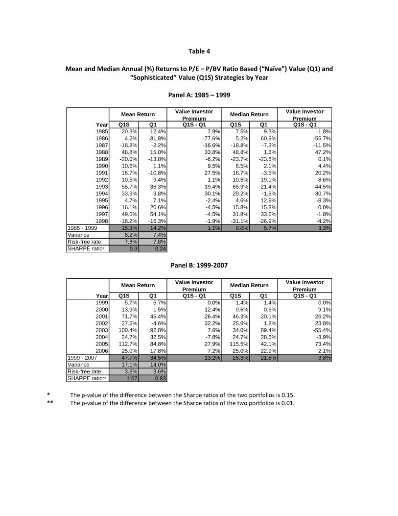
Table 4

Mean and Median Annual (%) Returns to P/E – P/BV Ratio Based (“Naïve”) Value (Q1) and “Sophisticated” Value (Q1S) Strategies by Year

Panel A: 1985 – 1999

Value Investor

Premium

Value Investor

Premium Year Q1S Q1 Q1S - Q1 Q1S Q1 Q1S - Q1

1985 20.3% 12.4% 7.9% 7.5% 9.3% -1.8%

1986 4.2% 81.8% -77.6% 5.2% 60.9% -55.7%

1987 -18.8% -2.2% -16.6% -18.8% -7.3% -11.5%

1988 48.8% 15.0% 33.8% 48.8% 1.6% 47.2%

1989 -20.0% -13.8% -6.2% -23.7% -23.8% 0.1%

1990 10.6% 1.1% 9.5% 6.5% 2.1% 4.4%

1991 16.7% -10.8% 27.5% 16.7% -3.5% 20.2%

1992 10.5% 9.4% 1.1% 10.5% 19.1% -8.6%

1993 55.7% 36.3% 19.4% 65.9% 21.4% 44.5%

1994 33.9% 3.8% 30.1% 29.2% -1.5% 30.7%

1995 4.7% 7.1% -2.4% 4.6% 12.9% -8.3%

1996 16.1% 20.6% -4.5% 15.8% 15.8% 0.0%

1997 49.6% 54.1% -4.5% 31.8% 33.6% -1.8%

1998 -18.2% -16.3% -1.9% -31.1% -26.9% -4.2%

1985 - 1999 15.3% 14.2% 1.1% 9.0% 5.7% 3.3%

Variance 6.2% 7.4%


SHARPE ratio* 0.3 0.24


Panel B: 1999-2007

Value Investor

Premium

Value Investor

Premium Year Q1S Q1 Q1S - Q1 Q1S Q1 Q1S - Q1

1999 5.7% 5.7% 0.0% 1.4% 1.4% 0.0%

2000 13.9% 1.5% 12.4% 9.6% 0.6% 9.1%

2001 71.7% 45.4% 26.4% 46.3% 20.1% 26.2%

2002 27.5% -4.6% 32.2% 25.6% 1.8% 23.8%

2003 100.4% 92.8% 7.6% 34.0% 89.4% -55.4%

2004 24.7% 32.5% -7.8% 24.7% 28.6% -3.9%

2005 112.7% 84.8% 27.9% 115.5% 42.1% 73.4%

2006 25.0% 17.8% 7.2% 25.0% 22.9% 2.1%

1999 - 2007 47.7% 34.5% 13.2% 25.3% 21.5% 3.8%

Variance 17.1% 14.0%


SHARPE ratio** 1.07 0.83


* The p-value of the difference between the Sharpe ratios of the two portfolios is 0.15. ** The p-value of the difference between the Sharpe ratios of the two portfolios is 0.01.

Table 5

Percentage of Positive and Negative Returns by P/E ‐ P/BV Ratio Based Naïve Value (Q1) and

Sophisticated Value (Q1S) Strategies

Panel A: 1985 – 1999

Year

% of negative

returns

% of positive

returns

% of negative

returns

% of positive

returns

1985 0.0% 100.0% 25.0% 75.0%

1986 0.0% 100.0% 0.0% 100.0%

1987 100.0% 0.0% 66.7% 33.3%

1988 0.0% 100.0% 45.5% 54.5%

1989 100.0% 0.0% 70.0% 30.0%

1990 0.0% 100.0% 33.3% 66.7%

1991 0.0% 100.0% 50.0% 50.0%

1992 0.0% 100.0% 14.3% 85.7%

1993 0.0% 100.0% 25.0% 75.0%

1994 0.0% 100.0% 54.5% 45.5%

1995 50.0% 50.0% 35.7% 64.3%

1996 40.0% 60.0% 18.2% 81.8%

1997 28.6% 71.4% 16.7% 83.3%

1998 75.0% 25.0% 69.2% 30.8%

Q1S (Sophisticated) Q1 (Value)

Panel B: 1999-2007

Year

% of negative

returns

% of positive

returns

% of negative

returns

% of positive

returns

1999 50.0% 50.0% 50.0% 50.0%

2000 33.3% 66.7% 50.0% 50.0%

2001 0.0% 100.0% 0.0% 100.0%

2002 0.0% 100.0% 37.5% 62.5%

2003 0.0% 100.0% 0.0% 100.0%

2004 0.0% 100.0% 0.0% 100.0%

2005 0.0% 100.0% 18.2% 81.8%

2006 25.0% 75.0% 25.0% 75.0%


Table 6

Mean and Median Market Cap ($Mil.) to P/E – P/BV Ratio Based Naïve Value (Q1) and Sophisticated Value (Q1S) Strategies by Year

Panel A: 1985 – 1999


1985 54.78 54.59 101.76 78.11

1986 43.62 29.03 42.97 26.33

1987 23.92 23.92 260.3 75.77

1988 52.91 52.91 190.33 115.79

1989 687.23 220.32 260.38 79.58

1990 544.07 293.81 283.73 147.72

1991 32.1 32.1 132.87 46.56

1992 36.96 36.96 151.88 145.7

1993 159.99 62.46 130.93 52.87

1994 186.35 64.2 127.86 50.03

1995 138 25.68 89.2 63.8

1996 39.99 26.57 44.4 26.57

1997 100.75 32.11 99.1 52.1

1998 88.4 89.97 157.84 61.27


Panel B: 1999-2007


1999 34.18 33.78 44.55 26.85

2000 88.28 35.98 91.29 73.32

2001 77.36 37.94 97.14 47.01

2002 61.58 65.56 95.01 65.56

2003 81.08 76.54 143.94 147.69

2004 425.09 425.09 187.83 44.91

2005 51.74 55.9 262.97 71.89

2006 203.29 111.12 316.75 87.59


Table 7

Mean and Median Annual (%) Returns to P/E – P/BV Ratio Based Value (Q1) and Growth (Q16) Strategies by Year

2007-2009


Q1 Q16 Q1 – Q16 Q1 Q16 Q1 – Q16

2007 -30.20% 20.20% -50.40% -31.30% 9.60% -40.90%

2008 -58.20% -33.50% -24.70% -62.30% -34.40% -27.90%

2008 (Extended)* -31.20% -16.60% -14.60% -34.00% -14.60% -19.30%

Year


* May 1, 2008 - September 30, 2009.

Table 8

Mean and Median Annual (%) Returns to P/E – P/BV Ratio Based (“Naïve”) Value (Q1) and “Sophisticated” Value (Q1S) Strategies by Year

2007-2009

Value Investor

Premium

Value Investor

Premium

Q1S Q1 Q1S - Q1 Q1S Q1 Q1S - Q1

2007 -45.70% -30.20% -15.50% -45.70% -31.30% -14.40%

2008 -13.00% -58.20% 45.20% -13.00% -62.30% 49.30%

2008 (Extended)* 64.70% -31.20% 95.90% 64.70% -34.00% 98.70%

Median Return

Year

Mean Return

* May 1, 2008 - September 30, 2009.

Documents

Do Value Investors Add Value? - csinvesting.orgcsinvesting.org/.../2013/02/Do_Value_Investors_Add_Valueshort.pdfare Reyer Barel and Saj Karsan (1999-2006), Dalton Baretto, Scott Gryba,