DO TAX IMPLICATIONS CHANGE THE FISHER EFFECT …meea.sites.luc.edu/volume15/pdfs/Tax-Implications.pdf · DO TAX IMPLICATIONS CHANGE THE FISHER EFFECT FOR THE TURKISH ... while Evans

Topics in Middle Eastern and African Economies

Vol. 15, No. 2, September 2013

1

DO TAX IMPLICATIONS CHANGE THE FISHER EFFECT FOR THE TURKISH

ECONOMY?

Kenan Lopcu1 Nuran Coşkun

2 Süleyman Değirmen

3

Prepared for Presentation at the 33nd

Annual Meeting of the MEEA, ASSA

January 4-7, 2013, San Diego, CA

Abstract

This study investigates the validity of both the conventional and tax-adjusted Fisher

effects using time series methods such as the ARDL bounds test, and Gregory-Hansen (G-H)

cointegration test. To compare the conventional and tax-adjusted Fisher effects, we use two

different time series data for interest rates: 1) interest rates adjusted for taxes, and 2) interest

rates not adjusted for taxes. Using monthly changes in quarterly and annual interest and

inflation rates, both the G-H and ARDL bound tests support the conventional and tax-adjusted

Fisher effects. However, the magnitude of the inflation coefficient in the long-run relationship

tends to decline for the tax adjusted Fisher effect.

Keywords: Fisher Effect, Taxation, Time Series Methods

JEL Code: C22, E43

Introduction

The existence of the Fisher effect in a country is important in deciding whether

implemented economic policies are sustainable. When a country experiences deviations from

its targeted inflation rate due to shocks to the system, the nominal interest rate could be a

significant instrument for inflation targeting, given the cointegration between the nominal

interest rate and inflation. Thus, for countries like Turkey, which aims at price stability, the

nominal interest rate is a significant instrument for long-run inflation targeting.

The empirical validity of the Fisher effect has been restudied extensively in the

literature in the last several decades, mostly due to the development of time series methods

1 Çukurova University, Department of Econometrics, email: [email protected]

2Mersin University, Department of Economics, email: [email protected]

3 Mersin University, Department of Economics, email: [email protected]



2

dealing with non-stationary data. Researchers now have various cointegration (Engle-

Granger, Johansen) and VAR techniques in their hands to test the long-run relationship

between individually non-stationary series (Atkins and Coe, 2002). However, potential

shortcomings of these studies are 1) that these techniques require that individual series be

non-stationary; and 2) most of these studies test the existence of a conventional Fisher effect

rather than a tax-adjusted Fisher effect. The purpose of this study, then, is to test if the

conventional and tax-adjusted Fisher effects are valid for Turkey, one of the most dynamic

economies in the classification of developing countries. This study also aims to contribute to

the current literature by including tax adaptation in the nominal interest rate for a developing

country case. To that end, we use two different time series data for interest rates: 1) interest

rates adjusted for taxes, and 2) interest rates not adjusted for taxes. Time series methods such

as the ARDL bounds test of Pesaran, Shin and Smith (2001) and cointegration tests with a

structural break are used to determine if consistent results for the existence of the Fisher effect

can be reached.

In conclusion, for the post financial liberalization era in Turkey when tax adaptation

has been especially implemented, declines in the inflation rate are associated with declines in

the nominal interest rate. Therefore, in contrast to the findings for developed countries (see

Atkins & Coe, 2002), this study finds support in favor of both types of Fisher effects in

Turkey: the conventional and the tax-adjusted Fisher effect.

Theoretical Framework and Literature Review

Fisher (1930) hypothesized that the nominal interest rate was equal to the sum of the real

interest rate and the expected inflation rate. He claimed that the nominal interest rate is

comprised of the real interest rate and the expected inflation of the same period. Additionally,

the Fisher effect asserts that there is a linear relationship between the nominal interest rate and

the expected inflation, and assumes that the real interest rate does not change in the long run.

If the real interest rate is not affected by monetary imbalances that affect inflation in the long

term, this will cause a relationship between inflation and the nominal interest rate, leading to

the likely existence of cointegration between the nominal interest rate and inflation.

To test the Fisher effect we use a standard model often encountered in the literature

(e.g. Harrison (2010)):

)(infEintrealint 1tttt

According to the rational expectations;



3

)(infE 1tt - 1tinf = te

where E ( te ) = 0

Hence, the average expectational error is zero. Additionally, rational expectations

suggest that the prediction error is uncorrelated with all the variables in the information set at

the time of the prediction. Thus, substituting the realized inflation rate for the expected one

the Fisher equation and our model is then;

More generally, this equation should be written as follows for developing countries;

)1()r1()i1( 1ttt

11 ttttt rri

The 1ttr term is important for developing countries which have suffered from high inflation

rates. Fisher (1930) examined the relationship between nominal interest rates and the rate of

inflation for the U.S. and the U.K. using annual data over the 1890–1927 period for the US,

and the 1820–1924 period for the U.K. Though Fisher (1930) asserted that the nominal

interest rate and inflation should affect one another evenly, he failed at presenting this

relationship empirically as his results indicated significant deviations from the Fisher effect.

Mundell (1963) attributed Fisher’s empirical results to the inflationary process by

asserting that the inflationary process reduces the real rate through the wealth effect.

Similarly, Tobin (1965) stated that nominal interest rates should adjust less than one to one

due to inflationary pressures on the real interest rate. Darby (1975) and Feldstein (1976), on

the other hand, argue that the nominal interest rate would adjust more than one for one

( )1/(1 ) to the expected inflation rate due to the tax effect. Shome, Smith and Pinkerton

(1988) argued that risk-averse investors need a premium to compensate them for any risks.

Carmichael and Stebbing (1983) assumed that nominal interest rates on financial assets can be

considered constant over time and that the real interest rate moves inversely with inflation.

Engsted (1996) and Crowder and Hoffman (1996) found support for the tax-adjusted

Fisher effect for 13 OECD countries and the U.S., respectively. Carr, Pesando and Smith

(1976), in contrast, could not find any evidence that supports the tax-adjusted Fisher effect for

Canada while Atkins and Coe (2002) found evidence supportive of the conventional Fisher

effect for the U.S. and Canada, but rejected the tax-adjusted Fisher effect for Canada and

provided mixed results for the U.S. Evans and Lewis (1995) and Mishkin (1992) employed

t1ttt einfintrealint



4

Engle and Granger’s (1987) bivariate cointegration test. Nevertheless, Mishkin’s (1992)

results did not support the Fisher hypothesis, while Evans and Lewis (1995) results supported

the Fisher hypothesis only when regime shifts in the expected inflation process were taken

into account. Since 1994 Turkey has been applying income tax on nominal interest incomes.

In the event of a tax application on nominal interest incomes, the examination of the Darby-

Feldstein effect is important in terms of policy proposals in countries with inflation targeting

whose main instrument is short term interest rates.

For Turkey, Turgutlu (2004), Kesriyeli (1994), Şimşek and Kadılar (2006) and Köse et

al (2012) obtained findings supportive of the Fisher effect in Turkey. Additionally, Kasman et

al (2006) found results in favor of the presence of the Fisher effect in a large majority of 33

countries, including Turkey. All the mentioned studies for Turkey, however, excluded the tax

adjustment procedure, which led us to examine the tax adjusted Fisher effect for Turkey.

Data

This study examines the validity of the Fisher effect in Turkey over the period of 1990:01

through 2011:11. Interest rates are proxied by quarterly and annual deposit rates and are from

international financial statistics (IFS). Two different time series are used for nominal interest

rates:

i) Interest rates adjusted for taxes

ii) Interest rates not adjusted for taxes

The quarterly inflation rate is measured as the 3 month to 3 month percentage change

in the consumer price index (CPI) multiplied by 400. The annual inflation is measured as the

yearly change in the CPI multiplied by 100. Turkey has implemented income tax on interest

earnings since 1994. Tax rates are obtained from the decisions of the Council of Ministers.

Because no publicly available data exist for double taxation and tax immunities they cannot

be taken into account. So, the tax adjusted interest rates are only imperfect proxies of the

theoretical ones. Nevertheless, they are also the only ones that can be derived from the

existing data sources. Variable definitions, the period covered and the data sources are given

in Table 1.

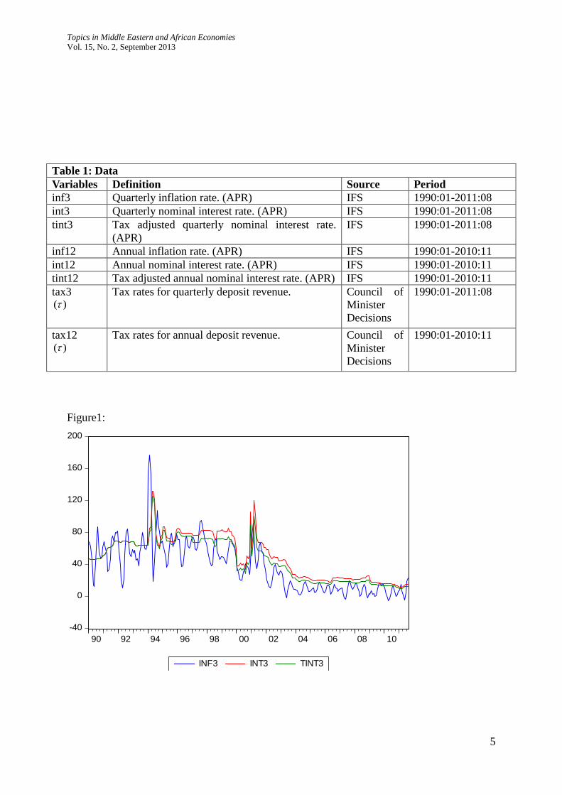
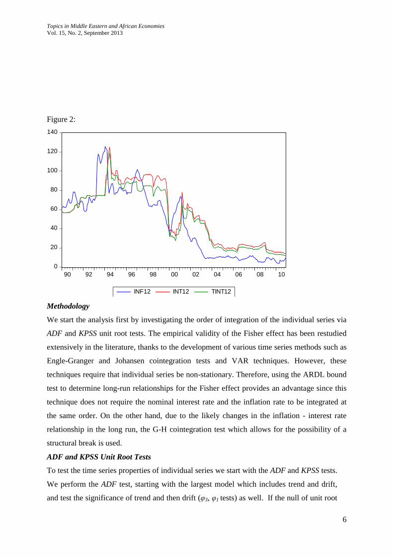
Quarterly and annual inflation, interest rate and the tax adjusted interest rate series are

shown in figures 1 and 2, respectively. According to the graphs, changes in interest rates

follow the changes in the inflation rate. This is particularly true for the crises periods of 1994

and 2001. These are also the periods where the interest rates tend to be negative or circa zero.

It is also noticeable that the declines in the inflation rate are associated with declines in

nominal interest rates in the last decade.



5

Table 1: Data

Variables Definition Source Period

inf3 Quarterly inflation rate. (APR) IFS 1990:01-2011:08

int3 Quarterly nominal interest rate. (APR) IFS 1990:01-2011:08

tint3 Tax adjusted quarterly nominal interest rate.

(APR)

IFS 1990:01-2011:08

inf12 Annual inflation rate. (APR) IFS 1990:01-2010:11

int12 Annual nominal interest rate. (APR) IFS 1990:01-2010:11

tint12 Tax adjusted annual nominal interest rate. (APR) IFS 1990:01-2010:11

tax3 )(

Tax rates for quarterly deposit revenue. Council of

Minister

Decisions

1990:01-2011:08

tax12 )(

Tax rates for annual deposit revenue. Council of

Minister

Decisions

1990:01-2010:11

Figure1:

-40

0

40

80

120

160

200

90 92 94 96 98 00 02 04 06 08 10

INF3 INT3 TINT3



6

Figure 2:

0

20

40

60

80

100

120

140

90 92 94 96 98 00 02 04 06 08 10

INF12 INT12 TINT12

Methodology

We start the analysis first by investigating the order of integration of the individual series via

ADF and KPSS unit root tests. The empirical validity of the Fisher effect has been restudied

extensively in the literature, thanks to the development of various time series methods such as

Engle-Granger and Johansen cointegration tests and VAR techniques. However, these

techniques require that individual series be non-stationary. Therefore, using the ARDL bound

test to determine long-run relationships for the Fisher effect provides an advantage since this

technique does not require the nominal interest rate and the inflation rate to be integrated at

the same order. On the other hand, due to the likely changes in the inflation - interest rate

relationship in the long run, the G-H cointegration test which allows for the possibility of a

structural break is used.

ADF and KPSS Unit Root Tests

To test the time series properties of individual series we start with the ADF and KPSS tests.

We perform the ADF test, starting with the largest model which includes trend and drift,

and test the significance of trend and then drift (φ3, φ1 tests) as well. If the null of unit root



7

and insignificant trend or drift cannot be rejected, we move to the next model. Lag lengths

are determined starting with the maximum length of 12 and reducing them until we find a

significant t-value for the individual lag. Since the ADF tests have low power, we also use

the KPSS tests to corroborate the results. For the KPSS tests both the trend and drift models

are used to test the null of no unit root, using Newey-West Bandwidth criteria with Barlett

kernel. However, neither of the above tests takes into account a potential structural break

when testing for a unit root. For that, we turn to the Zivot-Andrew (Z-A) (1992) unit root

test.

Zivot-Andrews Unit Root Test (Z-A)

Unit root tests can be biased if the structural breaks are not accounted for. Z-A (1992)

proposed a test that determines the break in the series endogenously. The individual series has

a unit root under the null and is trend stationary with a structural break at a time TB (1<TB<T)

under the alternative. The test is based on a procedure that trims a small percentage of the data

at two ends and calculates the t-value for each of the remaining observations as being the

potential break point. The observation with the smallest t-value, the least favorable outcome

for the null, then, is chosen as the break point. Z-A (1992) provided the critical values for the

test. Three different models are proposed for the test.

Model A permits one time change in the level of the series:

k

1j

tjt

A

j1t

AA

t

AA

t eycyt)(DUy

Model B allows one time change in the slope of the trend function occurring at time TB:

k

j

tjt

B

jt

BBt

BB

t eycytDTy1

1

* )(

Finally, Model C permits a onetime change both in the level and the trend of the series.

k

1j

tjt

C

j1t

Ct

*CC

t

CC

t eycy)(DTt)(DUy

DU(λ) , DT*(λ) are dummy variables, representing the change in the level and the trend of

the series:

otherwise ,0

TB,t ,1)(DUt

otherwise ,0

TB,t ,TB -t)(DT t

* TTB , and λ is the break

fraction.



8

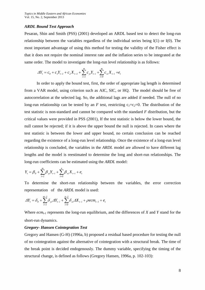
ARDL Bound Test Approach

Pesaran, Shin and Smith (PSS) (2001) developed an ARDL based test to detect the long-run

relationship between the variables regardless of the individual series being I(1) or I(0). The

most important advantage of using this method for testing the validity of the Fisher effect is

that it does not require the nominal interest rate and the inflation series to be integrated at the

same order. The model to investigate the long-run level relationship is as follows:

t

m

0i

itxi

m

1i

ityi1t21t10t eXcYcXcYccY

In order to apply the bound test, first, the order of appropriate lag length is determined

from a VAR model, using criterion such as AIC, SIC, or HQ. The model should be free of

autocorrelation at the selected lag. So, the additional lags are added if needed. The null of no

long-run relationship can be tested by an F test, restricting c1=c2=0. The distribution of the

test statistic is non-standard and cannot be compared with the standard F distribution, but the

critical values were provided in PSS (2001), If the test statistic is below the lower bound, the

null cannot be rejected; if it is above the upper bound the null is rejected. In cases where the

test statistic is between the lower and upper bound, no certain conclusion can be reached

regarding the existence of a long-run level relationship. Once the existence of a long-run level

relationship is concluded, the variables in the ARDL model are allowed to have different lag

lengths and the model is reestimated to determine the long and short-run relationships. The

long-run coefficients can be estimated using the ARDL model:

m

1i

n

0i

titxiityi0t eXYY

To determine the short-run relationship between the variables, the error correction

representation of the ARDL model is used:

1m

1i

1n

0i

t1titxiityi0t eecmXYY

Where ecmt-1 represents the long-run equilibrium, and the differences of X and Y stand for the

short-run dynamics.

Gregory- Hansen Cointegration Test

Gregory and Hansen (G-H) (1996a, b) proposed a residual based procedure for testing the null

of no cointegration against the alternative of cointegration with a structural break. The time of

the break point is decided endogenously. The dummy variable, specifying the timing of the

structural change, is defined as follows (Gregory Hansen, 1996a, p. 102-103):



9

,

,

n t if ,1

n t if ,0t

where n is the number of observations, τ (0,1) indicates the timing of the structural change

point and [ ] denotes the integer part. The four models proposed are as follow:

Model 1: Level Shift (C) Model

,eyy tt2

T

t211t t=1,…, n

This model allows a break in the intercept, where µ1 represents the intercept before the

break, and µ2 represents the change in the intercept at the time of the break.

Model 2: Level Shift with trend (C/T) Model

tt2

T

t211t eyty , t=1,…, n

This model takes the break into account in the intercept in the presence of a

deterministic trend.

Model 3: Regime Shift (C/S) Model

,eyyy t2tt

T

2t2

T

1t211t t=1,…, n.

The model does not include a deterministic trend, but permits a break in the intercept

as well as in the slope coefficients. µ1 and µ2 are as in Model 1, T

1 and T

2 , on the other

hand, represent the slope coefficients before the regime shift and the changes in the slope

coefficients after the regime change, respectively.

Model 4: Trend and Regime Shift (C/T/S) Model

,eyytty t2tt

T

22t

T

1t21t211t t=1,…, n

The model was proposed by G-H (1996b) and is the largest model which allows a

break in the level, trend and slope coefficients. µ1, β1, and T

1 represent the intercept, trend

and slope coefficients, respectively, before the regime change, µ2, β2 and T

2 , in contrast,

denote the changes in the parameters after the regime change.

The test is based on a procedure that trims a small percentage of the data at two ends

and calculates the ADF, and the Phillips (1987) Zα and Zt statistics for each of the remaining

observations as being the potential break point. The observation with the smallest test-value,

the least favorable outcome for the null, then, is chosen as the break point. Hence the three

test statistics proposed are as follows (Gregory and Hansen 1996a, b).

)ADF( minADFT

*

, )( ZminZT

*

,

)( ZminZ tT

*

t



10

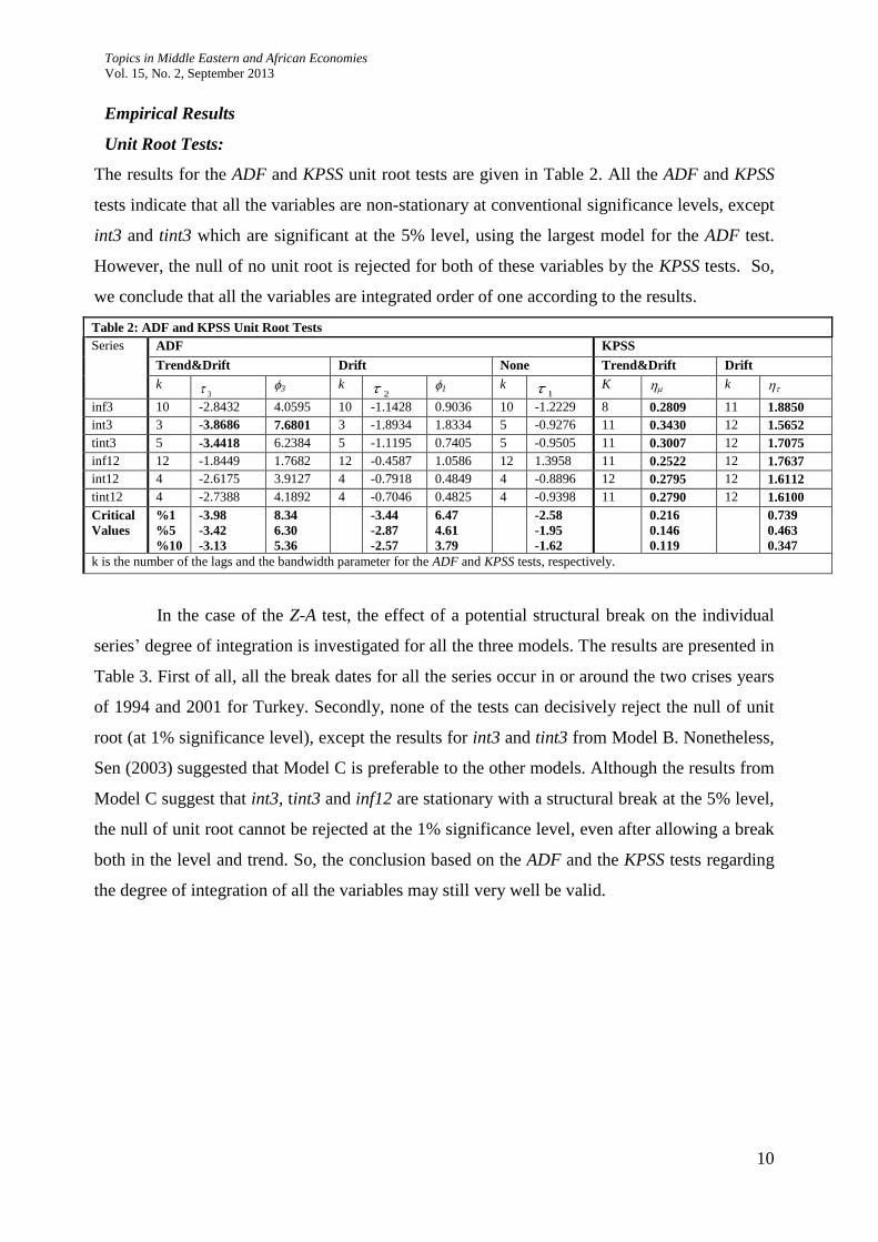
Empirical Results

Unit Root Tests:

The results for the ADF and KPSS unit root tests are given in Table 2. All the ADF and KPSS

tests indicate that all the variables are non-stationary at conventional significance levels, except

int3 and tint3 which are significant at the 5% level, using the largest model for the ADF test.

However, the null of no unit root is rejected for both of these variables by the KPSS tests. So,

we conclude that all the variables are integrated order of one according to the results.

Table 2: ADF and KPSS Unit Root Tests

Series ADF KPSS

Trend&Drift Drift None Trend&Drift Drift

k 3 3 k

2 1 k 1 K k

inf3 10 -2.8432 4.0595 10 -1.1428 0.9036 10 -1.2229 8 0.2809 11 1.8850

int3 3 -3.8686 7.6801 3 -1.8934 1.8334 5 -0.9276 11 0.3430 12 1.5652

tint3 5 -3.4418 6.2384 5 -1.1195 0.7405 5 -0.9505 11 0.3007 12 1.7075

inf12 12 -1.8449 1.7682 12 -0.4587 1.0586 12 1.3958 11 0.2522 12 1.7637

int12 4 -2.6175 3.9127 4 -0.7918 0.4849 4 -0.8896 12 0.2795 12 1.6112

tint12 4 -2.7388 4.1892 4 -0.7046 0.4825 4 -0.9398 11 0.2790 12 1.6100

Critical

Values

%1

%5

%10

-3.98

-3.42

-3.13

8.34

6.30

5.36

-3.44

-2.87

-2.57

6.47

4.61

3.79

-2.58

-1.95

-1.62

0.216

0.146

0.119

0.739

0.463

0.347

k is the number of the lags and the bandwidth parameter for the ADF and KPSS tests, respectively.

In the case of the Z-A test, the effect of a potential structural break on the individual

series’ degree of integration is investigated for all the three models. The results are presented in

Table 3. First of all, all the break dates for all the series occur in or around the two crises years

of 1994 and 2001 for Turkey. Secondly, none of the tests can decisively reject the null of unit

root (at 1% significance level), except the results for int3 and tint3 from Model B. Nonetheless,

Sen (2003) suggested that Model C is preferable to the other models. Although the results from

Model C suggest that int3, tint3 and inf12 are stationary with a structural break at the 5% level,

the null of unit root cannot be rejected at the 1% significance level, even after allowing a break

both in the level and trend. So, the conclusion based on the ADF and the KPSS tests regarding

the degree of integration of all the variables may still very well be valid.



11

Table 4-a : ARDL (4,10) for int3

Regressor Coefficient Standard Error T-Ratio[Prob]

inf3 0.96853 0.060533 16.00[.000]

C 13.8137 2.7836 4.96[.000]

95% Lower Bound 95% Upper Bound 90% Lower Bound 90% Upper Bound

4.9791 5.7037 5.7370 4.0755

F-statistic ARDL(4,4) 14.1673

ARDL(4,4): Serial Correlation:CHSQ(12) = 12.1411[.434]

F(12,226) = .96946[.479]

Table 4-b: ARDL(4,10) for tint3


tinf3 0.93717 0.049058 19.1033[.000]

C 10.1258 2.2563 4.4878[.000]


4.9791 5.7037 5.7370 4.0755


ARDL(1,1):Serial Correlation:CHSQ(12) = 19.8984[.069]

F(12,232) = 1.6865[.071]

Table 4-c: ARDL(5,3) for int12


inf12 0.93664 0.071472 13.1050[.000]

C 10.7852 4.1144 2.62[.009]


5.1343 5.6226 4.1847 4.7689



F(12,221) = .90655[.541]

Table 3: Zivot- Andrews Unit Root Test

Series Model A Model B Model C

K Test

statistic

TB DU

Prob.

K Test

statistic

TB DT

Prob.

K Test

statistic

TB DU

Prob.

DT Prob.

Inf3 10 -4.60 142 0.000 10 -3.66 49 0.023 10 -4.35 142 0.000 0.827

int3 3 -5.25 48 0.000 3 -5.25 52 0.000 3 -5.57 49 0.045 0.046

tint3 5 -4.52 136 0.001 3 -5.36 52 0.000 3 -5.55 49 0.110 0.041

Inf12 12 -3.09 133 0.007 12 -4.03 40 0.014 9 -5.10 133 0.000 0.937

int12 12 -3.09 133 0.007 12 -2.87 40 0.025 12 -3.04 37 0.196 0.473

tint12 1 -4.15 116 0.002 1 -3.78 50 0.014 1 -4.58 116 0.000 0.023

Critical

Values

%1

%5

%10

-5.34

-4.8

-4.58

-4.93

-4.42

-4.11

-5.57

-5.08

-4.82

k is the number of the lags determined by a significant t - ratio reduced from 12 and TB is the break point.



12

Table 4-d: ARDL(2,3) for tint12


inf12 0.86864 0.066707 13.0217[.000]

C 9.8691 3.8497 2.56[.011]


5.1343 5.6226 4.1847 4.7689



F(12,221) = .84999[.599]

Cointegration Test Results

The ARDL bound test results and the estimated long-run level relationships are displayed in

tables 4-a to 4-d. The calculated F-values are above the upper bounds in all cases, indicating

the existence of a long-run relationship between the nominal interest rate and the expected

inflation rate. The LM tests as well indicate that the errors are free of serial correlation at the

5% significance level. Once the cointegration relationship is verified, each model is

reestimated, allowing the right-hand variables to have different lag lengths. In all the cases the

point estimates for the expected inflation coefficients are slightly less than unity, but the 95%

confidence intervals contain unity. Thus, the ARDL results support both the conventional and

tax adjusted Fisher effect for Turkey.

In order to take into account a potential structural break in the long-run relationship,

we use the G-H cointegration test. The results are provided in Table 5. The G-H tests provide

a substantial support for cointegration with a structural break. In particular, using a 3-month

inflation and interest rate series, all three tests statistics reject the null of no cointegration for

all the structural change models and for both the tax adjusted and non-adjusted interest rates.

For the 12-month inflation and interest rate series, the ADF tests further verify the existence

of cointegration for all the models except the level shift (C) and the trend and the regime shift

(C/T/S) models.

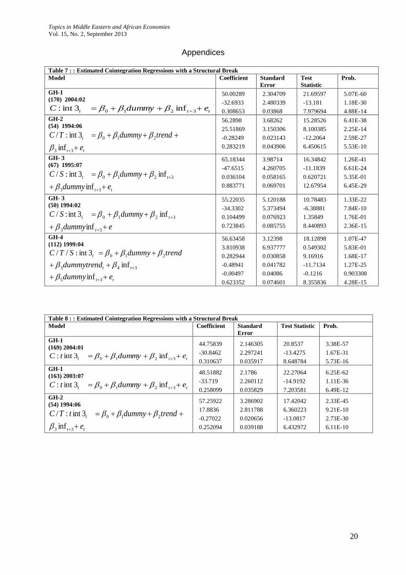
For the models where the null of no cointegration is rejected in favor of cointegration

with a structural break, we estimate the following regressions to see how the cointegration

relationships may have changed over time.

tkttt eEdummyC )(infint: 210

tkttt eEdummytrendTC )(infint:/ 3210

tkttttt edummyEEdummySC )(inf)(infint:/ 31210



13

t

kttttt

edummytrend

dummyEEdummytrendSTC

4

413210 )(inf)(infint://

where tintt would replace intt when the model is estimated for the tax adjusted Fisher effect.

Table 5 :Gregory Hansen Test Results

Model k ADF Break Point Zt Break Point Za Break Point

C (int3,inf3) 1 -7.27* 0.6538 (170) -6.57* 0.6538 (170) -76.03* 0.6538 (170)

C/T (int3,inf3) 1 -7.43* 0.2076 (54) -6.55* 0.2076 (54) -74.25* 0.2076 (54)

C/S (int3,inf3) 1 -7.36* 0.2576 (67) -8.24* 0.1923 (50) -112.47* 0.1923 (50)

C/T/S (int3,inf3) 1 -7.47* 0.4307 (112) -7.19* 0.4307 (112) -88.61* 0.4307 (112)

C (tint3,inf3) 1 -7.55* 0.6500 (169) -6.61* 0.6269 (163) -77.18* 0.6269 (163)

C/T (tint3,inf3) 1 -7.47* 0.2076(54) -6.52* 0.2000 (52) -73.37* 0.2000 (52)

C/S (tint3,inf3) 1 -7.70* 0.35384 (92) -8.21* 0.1923 (50) -112.35* 0.1923 (50)

C/T/S (tint3,inf3) 1 -7.27* 0.43076 (112) -6.96* 0.4307 (112) -83.57* 0.4307 (112)

C (int12,inf12) 9 -4.21 0.59362 (149) -4.02 0.2191 (55) -32.08 0.2191 (55)

C/T (int12, inf12) 9 -5.13* 0.23505 (59) -4.21 0.2191 (55) -34.09 0.2191 (55)

C/S (int12, inf12) 9 -5.07* 0.15139 (38) -4.20 0.1832 (46) -34.70 0.1832 (46)

C/T/S (int12, inf12) 9 -5.27* 0.49800 (125) -4.63 0.4581 (115) -41.51 0.4581 (115)

C (tint12, inf12) 9 -4.85* 0.71314 (179) -3.86 0.2191 (55) -29.75 0.2191 (55)

C/T (tint 12, inf12) 9 -5.09* 0.25498 (64) -4.05 0.2191 (55) -31.52 0.2191 (55)

C/S (tint 12, inf12) 9 -4.89* 0.72509 (182) -4.04 0.1832 (46) -32.17 0.1832 (46)

C/T/S (tint 12, inf12) 9 -5.04 0.49800 (125) -4.45 0.4541 (114) -38.46 0.4541 (114)

Critical Values

C

C/T

C/S

C/T/S

%1/5/10

%1/5/10

%1/5/10

%1/5/10

-5.13 / -4.61 / -4.34

-5.45 / -4.99 / -4.72

-5.47 / -4.95 / -4,68

-6.02 / -5.50 / -5.24

-5.13 / -4.61 / -4.34

-5.45 / -4.99 / -4.72

-5.47 / -4.95 / -4,68

-6.02 / -5.50 / -5.24

-50.07 / -40.48 / -36.19

-57.28 / -47.96 / -43.22

-57.17 /- 47.04 / -41.85

-69.37 / -58.58 / -53.31

Corresponding Break Dates

Observatio

n

Date Observation Date Observation Date Observation Date

38

46

50

52

54

1993:02

1993:10

1994:02

1994:04

1994:06

55

59

64

67

92

1994:07

1994:11

1995:04

1995:07

1997:08

112

114

115

125

149

1999:04

1999:06

1999:07

2000:05

2002:05

163

169

170

179

182

2003:07

2004:01

2004:02

2004:11

2005:02

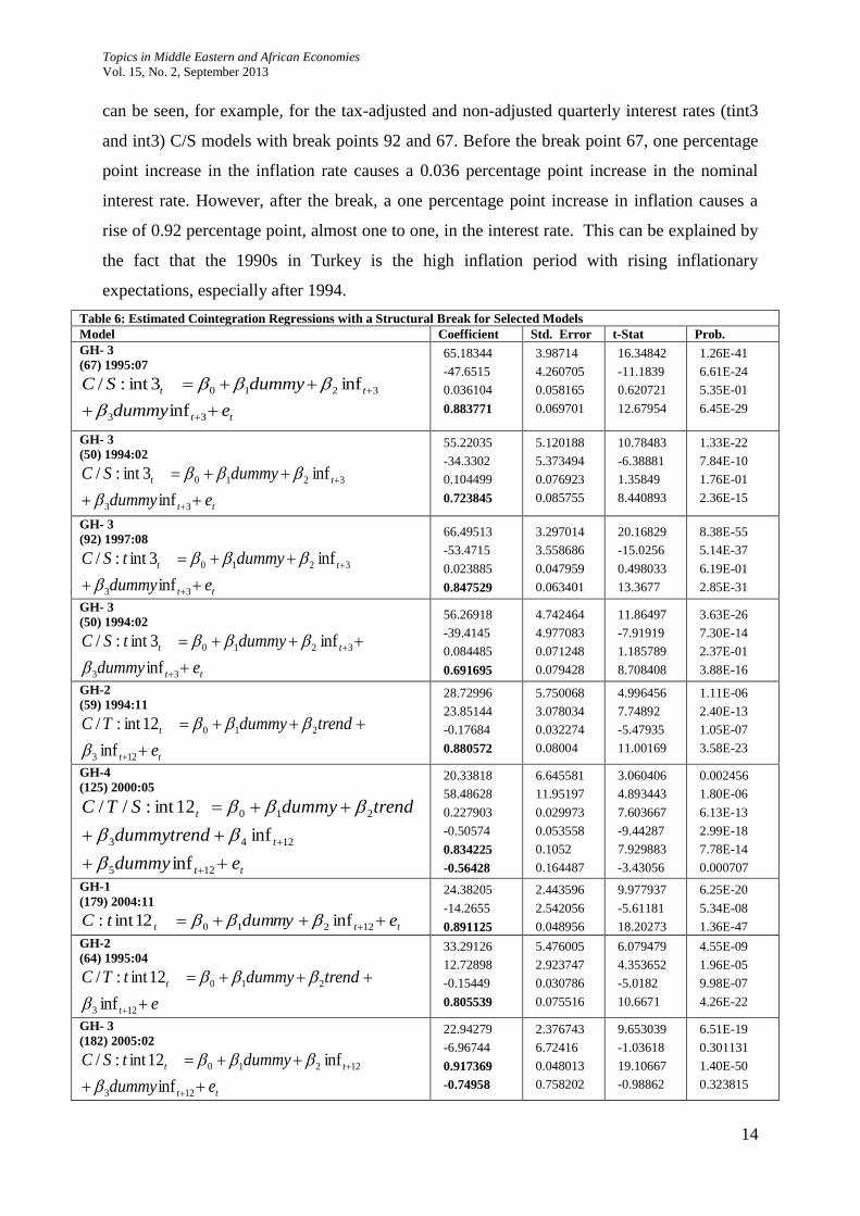
The results in Table 6 show that the effect of inflation on the nominal interest rate is

quite close to one both for the conventional and tax-adjusted Fisher effect at least in one of the

regimes. When the standard errors are taken into consideration, the presence of the Fisher

effect cannot be rejected. Endogenously determined break dates follow the 1994 and 2001

economic crises in general. Typically for breaks following the 1994 crisis the impact of

inflation on the nominal interest rate increases significantly and the Fisher effect holds. This



14

can be seen, for example, for the tax-adjusted and non-adjusted quarterly interest rates (tint3

and int3) C/S models with break points 92 and 67. Before the break point 67, one percentage

point increase in the inflation rate causes a 0.036 percentage point increase in the nominal

interest rate. However, after the break, a one percentage point increase in inflation causes a

rise of 0.92 percentage point, almost one to one, in the interest rate. This can be explained by

the fact that the 1990s in Turkey is the high inflation period with rising inflationary

expectations, especially after 1994.

Table 6: Estimated Cointegration Regressions with a Structural Break for Selected Models

Model Coefficient Std. Error t-Stat Prob.

GH- 3

(67) 1995:07

tt

tt

edummy

dummySC

33

3210

inf

inf3int:/

65.18344

-47.6515

0.036104

0.883771

3.98714

4.260705

0.058165

0.069701

16.34842

-11.1839

0.620721

12.67954

1.26E-41

6.61E-24

5.35E-01

6.45E-29

GH- 3

(50) 1994:02

tt

tt

edummy

dummySC

33

3210

inf

inf3int:/

55.22035

-34.3302

0.104499

0.723845

5.120188

5.373494

0.076923

0.085755

10.78483

-6.38881

1.35849

8.440893

1.33E-22

7.84E-10

1.76E-01

2.36E-15

GH- 3

(92) 1997:08

tt

tt

edummy

dummytSC

33

3210

inf

inf3int:/

66.49513

-53.4715

0.023885

0.847529

3.297014

3.558686

0.047959

0.063401

20.16829

-15.0256

0.498033

13.3677

8.38E-55

5.14E-37

6.19E-01

2.85E-31

GH- 3

(50) 1994:02

tt

tt

edummy

dummytSC

33

3210

inf

inf3int:/

56.26918

-39.4145

0.084485

0.691695

4.742464

4.977083

0.071248

0.079428

11.86497

-7.91919

1.185789

8.708408

3.63E-26

7.30E-14

2.37E-01

3.88E-16

GH-2

(59) 1994:11

tt

t

e

trenddummyTC

123

210

inf

12int:/

28.72996

23.85144

-0.17684

0.880572

5.750068

3.078034

0.032274

0.08004

4.996456

7.74892

-5.47935

11.00169

1.11E-06

2.40E-13

1.05E-07

3.58E-23

GH-4

(125) 2000:05

tt

t

t

edummy

dummytrend

trenddummySTC

125

1243

210

inf

inf

12int://

20.33818

58.48628

0.227903

-0.50574

0.834225

-0.56428

6.645581

11.95197

0.029973

0.053558

0.1052

0.164487

3.060406

4.893443

7.603667

-9.44287

7.929883

-3.43056

0.002456

1.80E-06

6.13E-13

2.99E-18

7.78E-14

0.000707

GH-1

(179) 2004:11

ttt edummytC 12210 inf12int:

24.38205

-14.2655

0.891125

2.443596

2.542056

0.048956

9.977937

-5.61181

18.20273

6.25E-20

5.34E-08

1.36E-47

GH-2

(64) 1995:04

e

trenddummytTC

t

t

123

210

inf

12int:/

33.29126

12.72898

-0.15449

0.805539

5.476005

2.923747

0.030786

0.075516

6.079479

4.353652

-5.0182

10.6671

4.55E-09

1.96E-05

9.98E-07

4.26E-22

GH- 3

(182) 2005:02

tt

tt

edummy

dummytSC

123

12210

inf

inf12int:/

22.94279

-6.96744

0.917369

-0.74958

2.376743

6.72416

0.048013

0.758202

9.653039

-1.03618

19.10667

-0.98862

6.51E-19

0.301131

1.40E-50

0.323815



15

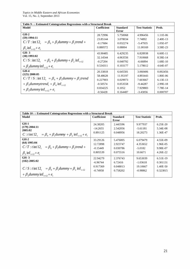
An opposite picture arises for the break points around or after 2001. In this case the impact of

inflation on the interest rate becomes weaker after the break. This can be attributed to

decreasing inflationary expectations as the last decade is a relatively lower inflation period.

See for example the C/S model for the tax-adjusted and non-adjusted annual interest rates

(tint12, int12) with break points 182 and 125.

Conclusion

This study investigated the conventional and tax adjusted Fisher effect for Turkey to humbly

suggest a policy for an incumbent government. Because the real interest rate for developed

small open economy countries is closer to the world interest rate in comparison to developing

countries, it is reasonable to expect that the Darby and Feldstein effect should apply for the

developed countries.

Mundell (1963) and Tobin (1965) indicated that inflation would affect the real

monetary stability when the economic agents prefer holding other assets rather than money

due to the increase in the anticipated inflation. This would lower the nominal rates instantly.

With regard to the Mundell-Tobin effect for tax implications, the welfare loss caused by the

inflationary process can be the reason for the tendency of inflation coefficients to be lower

than unity in the Fisher equation.

In this study, using the CPI-based inflation rate and the tax-adjusted and non-adjusted

deposit rates, we investigated the validity of the Fisher effect with the ARDL bounds test and

the Gregory-Hansen cointegration test. The results from the ARDL method are, in general,

supportive of both the conventional and tax-adjusted Fisher effects, but the magnitude of the

inflation coefficients tends to decline for the tax adjusted Fisher effect. The G-H tests provide

substantial evidence for the existence of the cointegration relationship between the expected

inflation and the nominal interest rate. However, about half the coefficients for the inflation

rate in the cointegration relationships are less than unity and do not significantly change for

the tax adjusted Fisher effect, a fact in contradiction to the Darby-Feldstein effect, but

compatible with Mundell-Tobin effect.

Real interest rates in Turkey have been above the world interest rate in the post

financial liberalization era. Hence, investors may continue to prefer investing in TL assets as

long as real interest rates are higher than the rest of the world. According to the results from

the G-H cointegration regressions, tax implications on the nominal interest rate do not affect

the saving behavior. Therefore, public revenues (taxes) should be obtained with direct rather

than indirect taxation for price stability and lower inflation.



16

It should be noted that deposit interest rates do not account for exceptional cases such

as tax immunities and double taxation. Savings deposits are preferred by small investors

rather than professional ones. Therefore, the results here should be compared with results

using other measures of nominal interest rates such as Treasury bill rates. Furthermore, the G-

H test was designed to account for only a single structural break. The results might be biased,

if there are multiple breaks, given the two important economic crises (1994, 2001) in the last

two decades, it very likely that the Fisher equation in Turkey had suffered more than one

structural break (see Figure 2, p. 6). So, the results here should be interpreted with caution.

Future research is needed to scrutinize the Fisher effect further with multiple structural breaks

and the alternative measures of interest rates.



17

References:

Atkins, F. and Coe, P.J. (2002), “An ARDL bounds test of the long-run Fisher effect in the

United States and Canada,” Journal of Macroeconomics, 24(2), 255-266.

Carr, J., Pesado, J.E. and Smith, L.B. (1976), “Tax effects, price expectations and the nominal

rate of interest,” Economic Inquiry, 14, 259- 269.

Carmichael, J., & Stebbing, P. W. (1983). “Fisher's paradox and the theory of interest.” The

American Economic Review, 619-630.

Crowder, W.J. (1997), “The long-run Fisher relation in Canada,” Canadian

Journal of Economics, 30(4), 1124-1142.

Crowder, W.J. and Hoffman, D.L. (1996), “The Long-run relationship between nominal

interest rates and inflation: The Fisher equation revisited,” Journal of Money,

Credit, and Banking, 28(1), 102-118.

Crowder, W.J. and Wohar, M.E. (1999), “Are tax effects important in the longrun Fisher

relationship? Evidence from the municipal bond market,” Journal of Finance,

54(1), 307-317.

Dickey, D. A. and Fuller, W. A. (1979), “Distribution of the estimators for autoregressive

time Series with a unit root,” Journal of the American Statistical Association, 74, 427-

431.

Darby, M.R. (1975), “The financial and tax effects of monetary policy on interest rates,”

Economic Inquiry, 13(2), 266-276.

Engle, R. F., and Granger, C. W. 1987. “Co-integration and error correction: representation,

estimation, and testing.” Econometrica, 55(2) 251-276.

Engsted, T. (1996), “Non-stationarity and tax effects in the long-term Fisher Hypothesis,”

Applied Economics, 28(7), 883-887.

Evans, M. D. D, and Lewis K. K. (1995) "Do long-term swings in the dollar affect estimates

of the risk premia?" Review of Financial Studies 8 (3),709-742.

Fama, E.F. (1975), “Short-term interest rates as predictors of inflation,” American Economic

Review, 65(3), 269-82.

Feldstein, M. (1976), “Inflation, income tax and the rate of interest: A theoretical analysis,”

American Economic Review, 66, 809-820.

Fisher, I. (1930), The Theory of Interest, New York: Macmillan.

Gregory, A.W. and Hansen, B. E. (1996), “Residual-based tests for cointegration in models

with regime shifts,” Journal of Econometrics, 70, 99–126.



18

Gregory, A. W., Nason, J.M. and Watt, D.G. (1994), “Testing for structural breaks in

cointegrated relationships,” Journal of Econometrics, 71(1), 321–341.

Harrison, M. (2010), “Valuing the Future: the social discount rate in cost-benefit analysis,”

Australian Government Productivity Commission.

Kasman, S., Kasman, A. and Turgutlu, E. (2006), “Fisher hypothesis revisited: a fractional

cointegration analysis,” Emerging Markets Finance Trade, 42, 59–76.

Köse, N., Emirmahmutoğlu, F. and Aksoy, S. (2012), “The interest rate- inflation relationship

under inflation targeting regime: The case of Turkey,” Journal of Asian

Economics, 840, 1-10.

Kesriyeli, M. (1994), “Policy regime changes and testing for the Fisher and UIP hypotheses:

The Turkish evidence,” The Central Bank of the Republic of Turkey, 9411.

Mishkin, F.S. (1992), “Is the Fisher effect for real? A reexamination of the relationship

between inflation and interest rates,” Journal of Monetary Economics, 30, 195-

215.

Mishkin, F.S. (2000), “Inflation targeting in emerging market countries,” American Economic

Review, 90,105-109.

Mundell, R. (1963), “Inflation and real interest,” Journal of Political Economy.

71, 280-283.

TCMB. (2006), Türkiye Cumhuriyeti Merkez Bankası Bilançosu Açıklamalar, Rasyolar ve

Para Politikası Yansımaları, TCMB, Ankara.

Perron, Pierre. (1989), “The great crash, the oil price shock, and the unit root hypothesis,”

Econometrica 57, 1361–401.

Pesaran, M. H. , Shin, Y. and Smith, R. J. (2001), “Bound testing approaches to the analysis

of long-run relationships,” Journal of Applied Econometrics, 16, 289-326.

Phillips, P. C. B. (1987), “Time series regression with a unit root,” Econometrica, 55, 277-

301.

Sen, A. (2003), “On unit root tests when the alternative is a trend break stationary process”,

Journal of Business and Economic Statistics, 21(1), 174-184.

Shome, D., Smith S., and Pinkerton, J. (1988) “The purchasing power of money and interest

rates: A re-examination,” Journal of Finance, 1113-1125.

Şimşek, M. and Kadılar, C. (2006), “Fisher etkisinin Türkiye verileri ile testi, Doğuş

Üniversitesi Dergisi, 7, 99-111.

Tobin, J. (1965), “Money and economic growth,” Econometrica, 33, 671-684.



19

Tobin, J. (1949), “Taxes, saving, and inflation,” The American Economic Review, 39(6),

1223-1232.

Turgutlu, E. (2004), “Fisher hipotezinin tutarlılığının testi: Parçalı durağanlık ve parçalı

kointegrasyon analizi,” D.E.İ.İ.B.F Dergisi, 19(2), 55-74.

Zivot E. and Andrews D. W. K. (1992), “Further evidence on the Great Crash, the oil-price

shock, and the unit-root hypothesis,” Journal of Business & Economic Statistics,

10 (3), 251-270.



20

Appendices

Table 7 : : Estimated Cointegration Regressions with a Structural Break

Model Coefficient Standard

Error

Test

Statistic

Prob.

GH-1

(170) 2004:02

ttt edummyC 3210 inf3int:

50.00289

-32.6933

0.308653

2.304709

2.480339

0.03868

21.69597

-13.181

7.979694

5.07E-60

1.18E-30

4.88E-14

GH-2

(54) 1994:06

tt

t

e

trenddummyTC

33

210

inf

3int:/

56.2898

25.51869

-0.28249

0.283219

3.68262

3.150306

0.023143

0.043906

15.28526

8.100385

-12.2064

6.450615

6.41E-38

2.25E-14

2.59E-27

5.53E-10

GH- 3

(67) 1995:07

tt

tt

edummy

dummySC

33

3210

inf

inf3int:/

65.18344

-47.6515

0.036104

0.883771

3.98714

4.260705

0.058165

0.069701

16.34842

-11.1839

0.620721

12.67954

1.26E-41

6.61E-24

5.35E-01

6.45E-29

GH- 3

(50) 1994:02

edummy

dummySC

t

tt

33

3210

inf

inf3int:/

55.22035

-34.3302

0.104499

0.723845

5.120188

5.373494

0.076923

0.085755

10.78483

-6.38881

1.35849

8.440893

1.33E-22

7.84E-10

1.76E-01

2.36E-15

GH-4

(112) 1999:04

tt

tt

t

edummy

dummytrend

trenddummySTC

35

343

210

inf

inf

3int://

56.63458

3.810938

0.282944

-0.48941

-0.00497

0.623352

3.12398

6.937777

0.030858

0.041782

0.04086

0.074601

18.12898

0.549302

9.16916

-11.7134

-0.1216

8.355836

1.07E-47

5.83E-01

1.68E-17

1.27E-25

0.903308

4.28E-15



Error

Test Statistic Prob.

GH-1

(169) 2004:01


44.75839

-30.8462

0.310637

2.146305

2.297241

0.035917

20.8537

-13.4275

8.648784

3.38E-57

1.67E-31

5.73E-16

GH-1

(163) 2003:07


48.51882

-33.719

0.258099

2.1786

2.260112

0.035829

22.27064

-14.9192

7.203581

6.25E-62

1.11E-36

6.49E-12

GH-2

(54) 1994:06

tt

t

e

trenddummytTC

33

210

inf

3int:/

57.25922

17.8836

-0.27022

0.252094

3.286902

2.811788

0.020656

0.039188

17.42042

6.360223

-13.0817

6.432972

2.33E-45

9.21E-10

2.73E-30

6.11E-10



21



Error


GH-2

(59) 1994:11

tt

t

e

trenddummyTC

123

210

inf

12int:/

28.72996

23.85144

-0.17684

0.880572

5.750068

3.078034

0.032274

0.08004

4.996456

7.74892

-5.47935

11.00169

1.11E-06

2.40E-13

1.05E-07

3.58E-23

GH- 3

(38) 1993:02

tt

tt

edummy

dummySC

123

12210

inf

inf12int:/

43.90485

32.14544

-0.27204

0.534311

6.429235

4.063556

0.040792

0.103177

6.828938

7.910668

-6.66894

5.178612

6.60E-11

8.58E-14

1.68E-10

4.64E-07

GH-4

(125) 2000:05

tt

tt

t

edummy

dummytrend

trenddummySTC

125

1243

210

inf

inf

12int://

20.33818

58.48628

0.227903

-0.50574

0.834225

-0.56428

6.645581

11.95197

0.029973

0.053558

0.1052

0.164487

3.060406

4.893443

7.603667

-9.44287

7.929883

-3.43056

0.002456

1.80E-06

6.13E-13

2.99E-18

7.78E-14

0.000707



Error


GH-1

(179) 2004:11

2005:02


24.38205

-14.2655

0.891125

2.443596

2.542056

0.048956

9.977937

-5.61181

18.20273

6.25E-20

5.34E-08

1.36E-47

GH-2

(64) 1995:04

tt

t

e

trenddummytTC

123

210

inf

12int:/

33.29126

12.72898

-0.15449

0.805539

5.476005

2.923747

0.030786

0.075516

6.079479

4.353652

-5.0182

10.6671

4.55E-09

1.96E-05

9.98E-07

4.26E-22

GH- 3

(182) 2005:02

tt

tt

edummy

dummytSC

123

12210

inf

inf12int:/

22.94279

-6.96744

0.917369

-0.74958

2.376743

6.72416

0.048013

0.758202

9.653039

-1.03618

19.10667

-0.98862

6.51E-19

0.301131

1.40E-50

0.323815

Documents

DO TAX IMPLICATIONS CHANGE THE FISHER EFFECT …meea.sites.luc.edu/volume15/pdfs/Tax-Implications.pdf · DO TAX IMPLICATIONS CHANGE THE FISHER EFFECT FOR THE TURKISH ... while Evans