Do Tax Cuts Starve the Beast? The Effect of Tax …...CHRISTINA D. ROMER and DAVID H. ROMER 141 11641-03a_Romer_rev3.qxd 8/14/09 12:50 PM Page 141 of a long-run tax cut is typically

139

CHRISTINA D. ROMERUniversity of California, Berkeley

DAVID H. ROMERUniversity of California, Berkeley

Do Tax Cuts Starve the Beast? The Effect of Tax Changes on Government Spending

ABSTRACT The hypothesis that decreases in taxes reduce future govern-ment spending is often cited as a reason for cutting taxes. However, becausetaxes change for many reasons, examinations of the relationship between over-all measures of taxation and subsequent spending are plagued by problems ofreverse causation and omitted variable bias. To derive more reliable estimates,this paper examines the behavior of government expenditure following legis-lated tax changes that narrative sources suggest are largely uncorrelated withother factors affecting spending. The results provide no support for the hypoth-esis that tax cuts restrain government spending; indeed, the point estimatessuggest that tax cuts increase spending. The results also indicate that the maineffect of tax cuts on the government budget is to induce subsequent legislatedtax increases. Examination of four episodes of major tax cuts reinforces theseconclusions.

In a speech urging passage of the 1981 tax cuts, President Ronald Reaganmade the following argument:

Over the past decades we’ve talked of curtailing government spending sothat we can then lower the tax burden. Sometimes we’ve even taken a run atdoing that. But there were always those who told us that taxes couldn’t becut until spending was reduced. Well, you know, we can lecture our childrenabout extravagance until we run out of voice and breath. Or we can curetheir extravagance by simply reducing their allowance.1

1. “Address to the Nation on the Economy,” February 5, 1981, p. 2. Quotations frompresidential speeches are from John T. Woolley and Gerhard Peters, The American PresidencyProject (www.presidency.ucsb.edu), an online database of presidential documents.

11641-03a_Romer_rev3.qxd 8/14/09 12:50 PM Page 139

This idea that cutting taxes will lead to a reduction in government spendingis often referred to as the “starve the beast” hypothesis: the most effectiveway to shrink the size of government is to reduce the revenue that feedsit. This view has been embraced not just by politicians but also by distin-guished economists from Milton Friedman to Robert Barro.2

Of course, the starve-the-beast hypothesis is not the only view of howtax cuts affect expenditure. Another possibility is that government spendingis determined with little or no regard to taxes, and thus does not respondto tax cuts. A third possibility is that tax cuts actually lead to increases inexpenditure. One way this could occur is through the “fiscal illusion” effectproposed by James Buchanan and Richard Wagner (1977) and by WilliamNiskanen (1978): a tax cut without an associated spending cut weakensthe link in voters’ minds between spending and taxes, and so leads themto demand greater spending. Another possible mechanism is “shared fiscalirresponsibility”: if supporters of tax reduction are acting without concernfor the deficit, supporters of higher spending may do the same (see, forexample, Gale and Orszag 2004).

The question of how tax cuts affect government spending is clearlyan empirical one. And, indeed, there have been attempts to investigatethe aggregate relationship between revenue and spending. However, suchexaminations of correlations cannot settle the issue. Changes in revenueoccur for a variety of reasons. Many changes are legislated, but many othersoccur automatically in response to changes in the economy. And legis-lated tax changes themselves are motivated by numerous factors. Some,such as many increases in payroll taxes, are driven by increases in cur-rent or planned spending. Others, such as tax cuts motivated by a beliefin the importance of incentives, are designed to raise long-run economicgrowth.

The relationship between revenue and spending is surely not independentof the causes of changes in revenue. For example, if spending-driven taxchanges are common, a regression of spending on revenue will almost cer-tainly show a positive correlation. But this relationship does not show thattax changes cause spending changes; causation, in fact, runs in the oppositedirection. To give another example, if automatic and legislated counter-cyclical tax changes are common, one might expect to see expenditure rising

140 Brookings Papers on Economic Activity, Spring 2009

2. See, for example, Milton Friedman, “Fiscal Responsibility,” Newsweek, August 7,1967, p. 68; Robert J. Barro, “There’s a Lot to Like about Bush’s Tax Plan,” Business Week,February 24, 2003, p. 28; Gary S. Becker, Edward P. Lazear, and Kevin M. Murphy, “TheDouble Benefit of Tax Cuts,” Wall Street Journal, October 7, 2003, p. A20.


after declines in revenue, because spending on unemployment insurance andother relief measures typically rises in bad economic times. In this case, bothrevenue and spending are being driven by an omitted variable: the state of the economy. These examples suggest that looking at the aggregaterelationship between revenue and spending without accounting for thecauses of revenue changes may lead to biased estimates of the effect ofrevenue changes on spending.

This paper therefore proposes a test of the starve-the-beast hypothesisthat accounts for the motivations for tax changes. In previous work (Romerand Romer 2009), we identified all significant legislated tax changes inthe United States over the period 1945–2007. We then used the narrativerecord—presidential speeches, executive branch documents, congressionalreports, and records of congressional debates—to identify the key motiva-tion and the expected revenue effects of each action. In this paper we useour classification of motivations to isolate those tax changes that can legit-imately be used to examine the effect of revenue changes on spending fromthose that are likely to give biased estimates. In particular, we focus on thebehavior of spending following tax changes enacted for long-run purposes.These are changes in taxes that are explicitly not tied to current spendingchanges or the current state of the economy. They are, instead, intended topromote various long-run objectives, such as spurring productivity growth,improving efficiency, or, as in the case of the 1981 Reagan tax cut, shrink-ing the size of government. Examining the behavior of government spendingfollowing these long-run tax changes should provide a relatively unbiasedtest of the starve-the-beast hypothesis.

We examine the relationship between real government expenditure andour measure of long-run tax changes in a variety of specifications. We findno support for the hypothesis that a relatively exogenous decline in taxeslowers future government spending. In our baseline specification, the esti-mates in fact suggest a substantial and marginally significant positive impactof tax cuts on government spending. The finding of a lack of support forthe starve-the-beast hypothesis is highly robust. The evidence of an opposite-signed effect, in contrast, is not particularly strong or robust.

The result that spending does not fall following a tax cut raises an obvi-ous question: how then does the government budget adjust in response tothe cut? One possibility is that what gives is not spending but the tax cutitself. To investigate this possibility, we examine the response of both taxrevenue and tax legislation to long-run tax cuts. We find that revenue fallsin response to a long-run tax cut in the short run but then recovers afterabout two years. Most of this recovery is due to the fact that a large part

CHRISTINA D. ROMER and DAVID H. ROMER 141


of a long-run tax cut is typically counteracted by legislated tax increaseswithin the next several years. As we discuss, the fact that policymakers areable to adjust on the tax side helps to explain why they do not adjust on thespending side.

Although there have been numerous long-run tax changes spread fairlyuniformly over the postwar era, four stand out as the largest and best known:the tax cut passed over President Harry Truman’s veto in the Revenue Actof 1948; the Kennedy-Johnson tax cut legislated in the Revenue Act of 1964;the Reagan tax cut contained in the Economic Recovery Tax Act of 1981;and the tax cuts passed (along with some countercyclical actions) underPresident George W. Bush in 2001 and 2003. As a check on our analysis, we examine these four episodes in detail. We find that the behavior ofspending and taxes in these extreme episodes is consistent with the aggre-gate regressions. Perhaps more important, we find that policymakers oftendid not even talk as if their spending decisions were influenced by revenuedevelopments. They did, however, often invoke the tax cuts as a motiva-tion for later tax increases. Finally, we find that concurrent develop-ments, namely wars, account for some of the rise in spending in theseepisodes. But other concurrent developments caused measured spendingchanges to understate the effects of the spending decisions made in theseepisodes. In particular, three of the four episodes featured decisions toexpand entitlement programs that had only modest short-term effects onspending but very large long-term effects. As a result, it appears unlikelythat the failure of total expenditure to fall after these tax cuts was due tochance or unobserved factors.

As mentioned above, ours is not the first study to investigate thestarve-the-beast hypothesis. The most common approach is some varia-tion of a regression of spending on lagged revenue; examples include thestudies by William Anderson, Myles Wallace, and John Warner (1986)and by Rati Ram (1988). More sophisticated versions of this methodol-ogy are pursued by Henning Bohn (1991) and Alan Auerbach (2000,2003). Bohn, focusing on a long sample period dominated by wartimebudgetary changes, examines the interrelationships between revenue andspending in a vector autoregression (VAR) framework that allows forcointegration between the two variables (see also von Furstenberg, Green,and Jeong 1986 and Miller and Russek 1990). Auerbach, focusing on recentdecades, studies the relationship between policy-driven changes in spend-ing (rather than all changes in spending) and past deficits or projectionsof what future deficits would be if policy did not change (see alsoCalomiris and Hassett 2002).



The results of these studies are mixed, but for the most part they suggestthat tax cuts are followed by reductions in spending. None of these studies,however, consider the different reasons for changes in revenue, and thusnone isolate the impact of independent tax changes on future spending.Indeed, our results point to a potentially important source of bias in studiesusing aggregate data. We find that the only type of legislated tax changesthat are systematically followed by spending changes in the same directionare ones motivated by decisions to change spending. Since causation in thesecases clearly does not run from the tax changes to the spending changes,this relationship is not informative about the starve-the-beast hypothesis.We also find that this type of tax change is sufficiently common to make theoverall relationship between tax changes and subsequent spending changessubstantially positive.3

The rest of the paper is organized as follows. Section I discusses thedifferent motivations for tax changes and identifies the types of tax actionsbest suited for testing the starve-the-beast hypothesis. Section II analyzesthe relationship between tax changes and government expenditure andincludes a plethora of robustness checks. Section III examines how changesin taxes affect future tax revenue and tax legislation. Section IV discussesspending and taxes in the four key episodes. Section V presents our conclu-sions and discusses the limitations of our analysis.

I. The Motivations for Legislated Tax Changes and Tests of the Starve-the-Beast Hypothesis

Legislated tax changes classified by motivation are a key input into our testsof the starve-the-beast hypothesis. Therefore, it is important to describe ourclassification of motivations and to discuss which types of tax changes arelikely to yield informative estimates of the effects of tax changes on gov-ernment spending. We also provide a brief overview of our identification


3. One can also test the starve-the-beast hypothesis indirectly. Perhaps the best-knownstudy of this type is Becker and Mulligan (2003). They show that under appropriate assump-tions, the same forces that would give rise to a starve-the-beast effect would cause a reductionin the efficiency of the tax system to reduce government spending. They therefore examinethe cross-country relationship between the efficiency of the tax system and the share of gov-ernment spending in GDP. Although they find a strong positive relationship, the correlationbetween efficiency and spending, like that between taxes and spending, may reflect reversecausation or omitted variables. That is, countries may invest in efficient tax systems becausethey desire high government spending, or a third factor, such as tolerance of intrusive gov-ernment or less emphasis on individualism, may lead both to a broader, more comprehensivetax system and to higher government spending.


of the motivations for tax changes and of our findings about the patterns oflegislated tax changes in the postwar era.

I.A. Classification of Motivations

Our classification and identification of the motivations for postwar legis-lated tax changes are described in detail in Romer and Romer (2009). Thatpaper shows that the motivations for almost all tax changes have fallen intofour broad categories.

One type of tax change consists of those motivated by contemporaneouschanges in spending. Often, policymakers will introduce a new program orsocial benefit and raise taxes at about the same time to pay for it. This wastrue, for example, in the mid-1950s when the interstate highway systemwas started, and in the mid-1960s when Medicare was introduced. The keyfeature of these changes is that the spending change is the impetus for thetax change. Typically, such changes are tax increases, but spending-driventax cuts are not unheard of.

A second type of tax change encompasses those made because policy-makers believe that economic growth in the near term will be above or belowits normal, sustainable level. A classic example of such a countercyclicalaction is the 1975 tax cut. Taxes were reduced because the economy wasin a severe recession and growth was predicted to remain substantially belownormal. Countercyclical actions can be either tax cuts or tax increases,depending on whether they are designed to counteract unusually slow orunusually rapid expected growth.

A third type of tax change consists of those made to reduce an inheritedbudget deficit. By definition, these changes are all increases. A classic exam-ple is the 1993 tax increase under President Bill Clinton. This increase wasundertaken not to finance a contemporaneous rise in spending, but to reducea persistent deficit caused by past developments.

The fourth type consists of tax changes intended to raise long-run eco-nomic growth. This is a broad category that includes changes motivated by arange of factors. What unites these changes is that they are all designedto improve the long-term functioning of the economy. The most com-mon motivation is a belief that lower tax rates will improve incentivesand thereby spur long-run growth. Another motivation is a belief in thebenefits of small government and a desire to return the people’s moneyto them; a third is a desire to improve the efficiency and equity of the taxsystem. Many of the most famous tax cuts, such as the 1964 Kennedy-Johnson tax cut and the Reagan tax cuts of the early 1980s, fall underthe general heading of tax changes aimed at raising long-run growth.



Most of these changes are cuts, but some of the tax reforms included inthis category increased revenue.

I.B. Which Tax Changes Are Useful for Testing the Starve-the-Beast Hypothesis?

This description of the different motivations for legislated tax changesmakes it clear that some changes are much more appropriate for testing thestarve-the-beast hypothesis than others. What are needed are tax changesthat are not systematically correlated with other factors influencing gov-ernment spending. An obvious implication is that spending-driven taxchanges are not appropriate observations to use. Causation in these episodesruns from the desired change in spending to the change in taxes. There is anomitted influence on spending—the prior decision to change spending—that is strongly correlated with these tax changes. Thus, if we have classifiedspending-driven tax changes correctly, there will be a positive correlationbetween these changes and spending changes by construction. Includingspending-driven tax changes in a regression of spending changes on taxchanges would therefore bias the results toward finding a starve-the-beast effect.

Similar reasoning suggests that examining spending changes followingcountercyclical and deficit-driven tax changes could also be problematic.In these cases, however, the likely bias is against the starve-the-beasthypothesis. In both cases there may be spending changes that are negativelycorrelated with the tax changes but not caused by them. Rather, both the taxand the spending changes may be caused by a third factor.

In the case of countercyclical actions, the third factor is the state of theeconomy. In bad economic times, policymakers may cut taxes and increasespending as a way of raising aggregate demand. Also, some types of spend-ing, such as unemployment compensation and public assistance, increaseautomatically in recessions. Thus, the relationship between taxes and spend-ing in these episodes may reflect discretionary and automatic responses tothe state of the economy, not a behavioral link between tax revenue andspending decisions.

In the case of deficit-driven tax changes, the unobserved third factor isa general switch to fiscal responsibility. Tax increases to reduce inheritedbudget deficits are often passed as parts of packages that include spendingreductions. The spending reductions are not caused by the tax increases;rather, both are driven by a desire to eliminate the deficit. Inclusion of suchpackages in a regression of spending changes on tax changes will tend tobias the results away from supporting the starve-the-beast hypothesis.



This concern may be more important in theory than in reality, however.Our narrative analysis of tax changes documents the spending reductionsagreed to in conjunction with deficit-driven tax changes. In almost everycase, the spending cuts were small relative to the tax increases. There-fore, although one may want to treat the behavior of spending followingdeficit-driven tax changes with caution, it may in fact yield relativelyunbiased estimates.

The tax changes that are surely the most appropriate for testing the starve-the-beast hypothesis are those taken to spur long-run growth. As describedabove, these tax changes are not made in response to current macroeconomicconditions or in conjunction with spending changes. As a result, they areexactly the kind of changes that proponents of the starve-the-beast hypoth-esis believe are likely to alter government spending.

To the degree that focusing on this type of tax change may lead to bias,it is likely to be in the direction of finding a positive effect of taxes onspending. The ideal experiment for testing the starve-the-beast hypothesiswould be a tax change resulting from factors that have no direct impact onspending. Our long-run tax changes, however, include tax cuts for whichthe possible induced reduction in future spending is sometimes cited asa motivation. As a result, there is a potential correlation between spend-ing and tax changes in these episodes driven by a third factor: a desirefor smaller government. Policymakers, in addition to cutting taxes to starvethe beast, may take other actions to achieve this goal. Because this possi-ble omitted variable bias works in the direction of supporting the starve-the-beast hypothesis, a finding of a positive relationship between taxesand spending would have to be treated with caution. Since we in fact find anegative relationship, there is less cause for concern. Also, our narrativeanalysis suggests that this potential bias is likely to be small. The desirefor smaller government is rarely the primary motivation for long-run taxchanges; a belief in the incentive effects of lower taxes is considerablymore common, for example.

I.C. Overview of the Narrative Analysis

The implementation and results of our narrative analysis of postwar taxchanges are described in Romer and Romer (2009). We use a detailedexamination of a wide range of policy documents to identify all significantlegislated tax changes over the period 1945–2007. We then identify themotivations policymakers gave for each action. We find that policymakerswere usually both quite explicit and remarkably unanimous in their statedreasons for undertaking tax actions. Only infrequently do they emphasize



multiple motivations. In these cases we divide the tax changes into piecesreflecting the different motivations.

We also use the narrative sources to estimate the revenue impacts of theactions. Specifically, we determine how policymakers expected the actionsto affect tax liabilities. Very often, tax bills change taxes in a number ofsteps. In these cases our baseline revenue estimates show changes in eachof the quarters the various provisions took effect.4

Figure 1 shows legislated postwar tax changes classified by motivation,measured by their expected revenue effects as a percent of nominal GDP.5

The top panel shows the long-run changes, which are the key actions forour purposes. The graph makes clear that the vast majority of long-run taxactions are cuts. It also makes clear that long-run tax changes have beenfairly evenly distributed over the postwar era. The largest were the 1948tax cut, the Kennedy-Johnson tax cut in the mid-1960s, the Reagan tax cutin the early 1980s, and the two Bush tax cuts in the early 2000s.

The bottom panel shows the other types of tax changes. Although the firsthalf of the postwar era saw a number of small, deficit-driven tax increases,the vast majority took place in the 1980s and early 1990s. Most of thedeficit-driven increases were passed to deal with the long-run solvency ofthe Social Security and Medicare systems. Spending-driven changes aretypically tax increases, and these were both frequent and relatively largein the first half of the postwar era. By far the largest were those in the Rev-enue Act of 1945 following the end of World War II, and those in the early1950s to pay for the Korean War. Many of the other changes in this categorywere related to expansions of Social Security. Finally, explicitly counter-cyclical tax changes were confined to the fairly short period 1966–75until they were resurrected as the reason for portions of the tax cuts in 2001and 2002.


4. Tax actions are often retroactive for a quarter or two. Such changes have a muchlarger effect on liabilities in the initial quarter than in subsequent ones. In terms of differ-ences, this results in a large movement in one direction in the initial quarter and a partiallyoffsetting movement in the next quarter. For this study, which examines the longer-runresponses of spending and future taxes, the short-run volatility caused by these changesmay unnecessarily complicate the analysis. We therefore ignore the retroactive changes informing our baseline estimates. Including the retroactive changes has almost no impact onany of the results, however.

5. The nominal GDP data are from the National Income and Product Accounts, table 1.1.5(downloaded February 17, 2008). Quarterly nominal GDP data are available only after 1947.We therefore normalize the one tax change in 1946 using the annual nominal GDP figure forthat year.


II. The Effect of Tax Changes on Expenditure

The previous section describes our identification of legislated tax changesmotivated by concern about long-run growth. This section investigatesthe relationship between these relatively exogenous tax changes and sub-sequent changes in government spending. It includes a detailed analysis


Long-run tax changes

–2

–1

1950 1960 1970 1980 1990 2000

1950 1960 1970 1980 1990 2000

0

1

2

–2

–1

0

1

2

Percent of GDP

Percent of GDP

Other tax changes

Spending-driven

Countercyclical

Deficit-driven

Source: Romer and Romer (2009).

Figure 1. Legislated Tax Changes Classified by Motivation, 1945–2007


of the robustness of the results. We also investigate the behavior of spend-ing following other types of tax changes to see if there is evidence of biaswhen these changes are included.

II.A. Specification and Data

To estimate the effects of tax changes on government spending, we beginby estimating, using quarterly data, a simple reduced-form regression ofthe form

where ΔE is the change in the logarithm of real government expenditureand ΔT is our measure of long-run tax changes (specifically, the expectedrevenue effects, as a percent of nominal GDP, of the tax changes we iden-tify as motivated by long-run considerations).

The key feature of long-run tax changes as we have defined them is thatthey are based on actions motivated by considerations largely unrelated tocurrent spending, current macroeconomic conditions, or an inherited budgetdeficit. Our discussion above of why such long-run changes provide thebest test of the starve-the-beast hypothesis suggests that they are unlikelyto have a substantial systematic correlation with other factors affectingspending. It is for this reason that our baseline specification includes nocontrol variables. However, it is certainly possible that there are correla-tions in small samples, or that the dynamics of the relationship betweentax changes and spending are more complicated than is expressed inequation 1. We therefore also consider a wide range of control variablesand a variety of more complicated specifications.

We include a number of lags of the tax variable to allow for the possibil-ity that the response of spending to tax changes is quite delayed or gradual.In our baseline specification we set the number of lags to 20, and so look atthe response of spending over a five-year horizon. Because the starve-the-beast hypothesis does not make predictions about the exact timing of thespending response, we focus on the cumulative effect at various horizons.We summarize the regression results by reporting the implied impact of atax cut of 1 percent of GDP on the path of expenditure (in logarithms). Forour baseline specification, the cumulative impact after n quarters is just thenegative of the sum of the coefficients on the contemporaneous value andfirst n lags of the tax variable. The starve-the-beast hypothesis predicts thattax cuts reduce spending. Therefore, the estimated cumulative impact of atax cut on expenditure should be negative if the hypothesis is correct.

( ) ,10

Δ = + Δ +−=∑E a b T et i t i ti

N



We use quarterly data on government expenditure from the NationalIncome and Product Accounts (NIPA). Our series on long-run tax changesrefers only to federal legislation. Therefore, we consider only the behaviorof federal expenditure. What the Bureau of Economic Analysis (BEA)calls “total expenditures,” however, includes two components that arenot appropriate to include in considering the response of spending to taxchanges. One is a deduction for the consumption of fixed capital (that is,depreciation). This largely reflects spending decisions in the distant pastand so almost surely cannot show a starve-the-beast response. Thus, wedo not subtract depreciation. The other component is interest payments ongovernment debt. For a given interest rate, interest payments rise withthe amount of debt. As a result, any tax cut that increases the deficit willalmost certainly increase interest payments. We therefore exclude this typeof spending. The resulting aggregate that we consider is thus total grossexpenditure less interest. For simplicity, we refer to this as total expendi-ture in what follows.6

The NIPA expenditure data are expressed in nominal terms. Deflatorsexist for some components, such as defense and nondefense purchases, butnot for others, especially those involving transfers. We therefore deflate totalgross expenditure less interest by the price index for GDP (NIPA table 1.1.4,downloaded February 22, 2008).

Our data on tax changes begin in 1945Q1, and the data on expenditure in1947Q1. Therefore, in the baseline specification, where we include 20 lagsof the tax variable, the earliest starting date for the regression is 1950Q1.However, previous work has found some evidence that the behavior andeffects of fiscal policy were unusual in the Korean War period (see, forexample, Blanchard and Perotti 2002 and Romer and Romer forthcoming).We therefore also report estimates for regressions starting in 1957Q1. Inboth cases we carry the regressions through 2007Q4.

II.B. The Effect of Long-Run Tax Changes on Total Expenditure

Table 1 shows the results of estimating equation 1 for total expendi-ture using 20 lags of the long-run tax variable over the full sample. Thecoefficient estimates for the individual lags fluctuate between positive and


6. Data on total expenditures, consumption of fixed capital, and interest payments arefrom NIPA table 3.2 (downloaded February 17, 2008). Because the BEA does not have dataon “net purchases of nonproduced assets” (which are normally a trivial component of totalexpenditures) until 1959Q3, before then we estimate total gross expenditure less interest asthe sum of current expenditure, gross government investment, and capital transfer payments,minus interest payments.


negative. As one would expect, few of the individual coefficients are statisti-cally significant. The overall fit of the regression is modest (R2 = 0.20).

Figure 2 summarizes the results by showing the implied response oftotal expenditure to a long-run tax cut of 1 percent of GDP, together with1-standard-error bands. There is no evidence of a starve-the-beast effect.The cumulative effect is negative in the quarter of the tax cut and thesubsequent three quarters, as the starve-the-beast hypothesis predicts, butvery small, and the t statistics do not rise above 0.6 in absolute value. Afterthat, the estimated cumulative effect is positive at every horizon exceptquarters 9 and 10, suggesting fiscal illusion or shared fiscal irresponsibility.

The estimated positive impact of the tax cut on spending is often sub-stantial. Since federal government spending averages roughly 20 percent ofGDP in our sample, a tax cut of 1 percent of GDP is equal to about 5 percent


Table 1. Estimated Impact of Tax Changes on Total Expenditurea

Variable Coefficient

Constant 0.72 (0.25)Tax change:

Lag 0 0.24 (0.85)Lag 1 0.40 (0.85)Lag 2 −0.11 (0.85)Lag 3 −0.28 (0.83)Lag 4 −0.92 (0.87)Lag 5 −1.50 (0.87)Lag 6 0.31 (0.87)Lag 7 −1.42 (0.75)Lag 8 2.63 (0.75)Lag 9 2.52 (0.75)Lag 10 −0.98 (0.75)Lag 11 −1.53 (0.74)Lag 12 −2.19 (0.76)Lag 13 −2.13 (0.76)Lag 14 −1.11 (0.76)Lag 15 0.47 (0.76)Lag 16 0.02 (0.76)Lag 17 −0.11 (0.74)Lag 18 0.51 (0.78)Lag 19 0.86 (0.78)Lag 20 0.20 (0.78)

R2 0.20Durbin-Watson statistic 1.90Standard error of the estimate 2.72

Source: Authors’ regression.a. The table reports estimates of equation 1 in the text using data for long-run tax changes only and defin-

ing expenditure as total gross expenditure less interest payments. The sample period is 1950Q1–2007Q4.Numbers in parentheses are standard errors.


of government spending. The point estimates suggest that a tax cut of thatmagnitude raises spending by 4 percent or more in quarters 13 through 20.That is, they suggest that spending eventually rises by almost the amountof the tax cut. However, the estimates are not very precise. The t statisticsfor the cumulative impact of the tax cut on spending at horizons of morethan three years are generally between 1.5 and 2, exceeding 2 for only onehorizon (quarter 14, for which the t statistic is 2.21).

II.C. Richer Dynamics

Our baseline results suggest that there is no discernable starve-the-beasteffect, and some evidence of shared fiscal irresponsibility, over a five-yearhorizon. But perhaps the main effects of tax changes occur with longer lags.Here we consider several approaches to allowing for more delayed effects.

ADDITIONAL LAGS. The most straightforward approach to examiningwhether tax changes have important effects at longer horizons is to includeadditional lags in equation 1. Of course, including more lags requires short-ening the sample period and estimating additional parameters. The top panelof figure 3 shows the results of including 40 lags of the tax variable in


–4

–2

0

2

4

6

8

10

Quarters after tax change

Percent

2 4 6 8 10 12 14 16 18

Source: Authorsí re gressions.a. Based on an ordinary least squares (OLS) regression of the quarterly change in the logarithm of real

total gross federal expenditure less interest payments on the contemporaneous value and 20 quarterly lags of the measure of long-run tax changes; the sample period is 1950Q1–2007Q4. Dashed lines indicate 1-standard-error bands.

Figure 2. Cumulative Impact of a Tax Cut of 1 Percent of GDP on Total Expenditure,Baseline Specificationa



–4

–2

0

2

4

6

8

10


Percent

4 8 12 16 20 24 28 32 36

OLS estimatesa

–4

–2

0

2

4

6

8

10


Percent

4 8 12 16 20 24 28 32 36

Two-variable VAR estimatesb

Source: Authors’ estimates.a. Regression is specified as in figure 2 but with 40 lags of the measure of long-run tax changes; the

sample period is 1955Q1–2007Q4.b. Impulse response function from a vector autoregression (VAR) using the logarithm of total expendi-

ture as defined in figure 2 and the measure of long-run tax changes; there are 12 lags, and the tax measure is ordered first.

Figure 3. Cumulative Impact of a Tax Cut of 1 Percent of GDP on Total Expenditure,Estimates over Longer Horizons



equation 1 and estimating the regression over the longest feasible sample(1955Q1–2007Q4). For horizons beyond five years, the estimated cumu-lative impact of a tax cut of 1 percent of GDP on total expenditure is alwayssmall, fluctuates between positive and negative, and is never remotely closeto statistically significant. Thus, this specification provides no evidence thattax cuts reduce government spending, but also fails to support the hypothesisthat they increase it.

A TWO-VARIABLE VECTOR AUTOREGRESSION. Our second approach to allow-ing for more complicated and potentially longer-lasting dynamics is to esti-mate a VAR with our series for long-run tax changes and total expenditure.This approach allows spending to depend on its own lags as well as on thetax changes, and so allows for dynamics beyond the number of lags of thetax variable that are included.

For consistency with the earlier regressions, we put the tax changes firstand expenditure second, so that tax changes can affect spending withinthe quarter. We enter expenditure in logarithms; given the availability ofthe data, we can include 12 lags while still using our baseline sample. Thebottom panel of figure 3 shows that the estimated response of spending toan innovation of −1 percent of GDP to our series on long-run tax changesis similar to that for a long-run tax cut of 1 percent of GDP in the baselinespecification.7 The point estimates suggest that the tax cut reduces spend-ing in the short run but then raises it, with a fairly large positive long-runeffect. None of the estimated effects are statistically significant, however.Thus, again there is no support for the starve-the-beast hypothesis. Anotherfinding from the VAR is that the estimated response of the tax series to aninnovation to government spending is very small and highly insignificantat all horizons. This indicates that the actions we classify as long-run taxchanges are not responses to spending developments.8

7. Note that this experiment is slightly different from that considered in summarizingthe results from the baseline specification. There we consider a one-time tax cut of 1 percentof GDP with no further tax changes. Here, following the innovation to our tax measure in theVAR, there are on average additional long-run tax cuts of about one-fifth of a percent ofGDP over the next several years. We compute the standard errors by taking 10,000 draws ofthe vector of coefficient estimates from a multivariate normal distribution with mean andvariance-covariance matrix given by the point estimates and variance-covariance matrix ofthe coefficient estimates, and then finding the standard deviation of the implied responses ateach horizon.

8. We also estimated the bivariate VAR with 20 lags for the period 1952Q1–2007Q4.The estimated effects of a tax cut on spending in this specification are even more consistentlypositive and are marginally significant. The maximum effect is an increase of 3.97 percentafter 18 quarters (t = 1.93).


LARGER SYSTEMS. Another way that a starve-the-beast effect could occurat longer horizons is if tax cuts affect other variables that in turn affectgovernment spending. We therefore consider VARs with additional vari-ables. This, however, requires either estimating more parameters in eachequation or including fewer lags. Thus, rather than just include a long listof variables that might be relevant, we consider various combinations ofvariables.

One way that tax cuts could create pressures for reduced governmentspending is by increasing government debt. Thus, our first multivariableVAR uses three variables: our series on long-run tax changes, log realspending, and log real debt.9

We also consider two four-variable VARs. In one, we add the log ofreal federal total receipts as the fourth variable, so that the system includesboth the spending and the revenue sides of the government budget. In theother, the fourth variable is log real GDP. Our reason for including thisvariable is that tax cuts have large short-run effects on output (Romer andRomer forthcoming), which could in turn affect the dynamics of spendingin response to a tax cut.10

Finally, the nominal interest rate and inflation also affect the govern-ment budget constraint. Our last system is therefore a VAR with sevenvariables: our long-run tax series, log real spending, log real debt, log realrevenue, log real GDP, the three-month Treasury bill rate, and the log ofthe price index for GDP.11 In all of the VARs we put the tax series first, sothat it can affect the other variables within the quarter. We include 12 lagsand use the full sample (1950Q1–2007Q4).


9. From 1970Q1 to the end of the sample, we use quarterly data on the stock of fed-eral debt held by the public. From the beginning of the sample to 1969Q4, we use theavailable series on gross federal debt held by the public for the second quarter of eachyear, and we interpolate linearly between the annual observations. Both series are takenfrom the St. Louis Federal Reserve Bank’s FRED database, series FYGFDPUN andFYGFDPUB (www.stls.frb.org, downloaded March 24, 2008). We ratio-splice the twoseries in 1970Q2 and deflate the resulting series by the price index for GDP. Note thatsince it is likely to be the level of debt, rather than the change, that affects spending, theerrors caused by the interpolation in the first part of the sample should have only minoreffects on the estimates.

10. For receipts we use the federal total receipts series from NIPA table 3.2 (down-loaded April 6, 2009), deflated by the price index for GDP from NIPA table 1.1.4. Our real GDP series is the quantity index for GDP from NIPA table 1.1.3 (downloadedFebruary 17, 2008).

11. Data on the three-month Treasury bill rate are from the Board of Governors, seriesH15/H15/RIFSGFSM03_N.M (monthly data for secondary market rates on a discount basis,downloaded February 15, 2008).



12. In each of the VARs, following the innovation to the tax series, there are modestadditional long-run tax cuts over the next year that are largely offset over the following fewyears. There is never an important response of the tax variable to the other variables.

–4

0

4

8


PercentThree-variable VARa

4 8 12 16 20 24 28 32 36

–4

0

4

8


PercentFour-variable VAR including receiptsb

4 8 12 16 20 24 28 32 36

Figure 4. Cumulative Impact of a Tax Cut of 1 Percent of GDP on Total Expenditure,Multivariate VAR Estimates

Figure 4 displays the response of government spending to an innova-tion of −1 percent of GDP to our series on long-run tax changes in each ofthe VARs.12 The results consistently fail to support the starve-the-beasthypothesis. In every specification, the estimated effect of a tax cut on spend-ing is negative at only a few horizons. And in every case, those estimatesare small and insignificant: at no horizon is the t statistic for the spendingresponse negative and greater than 1 in absolute value. Adding debt to thebaseline VAR (first panel) in fact moves the estimates further in the direc-tion of suggesting fiscal illusion. The estimated maximum effect of the taxcut is an increase in spending of 5.75 percent (t = 2.12) after 17 quarters, andthe estimated effect after 10 years is an increase of 3.93 percent (t = 1.70).In the four-variable and seven-variable systems, the point estimates sug-gest a slightly weaker fiscal illusion effect, although it is more precisely



–4

0

4

8


PercentFour-variable VAR including GDPc

4 8 12 16 20 24 28 32 36

–4

0

4

8


PercentSeven-variable VARd

4 8 12 16 20 24 28 32 36

Source: Authors’ estimates.a. VAR includes the measure of long-run tax changes, the logarithm of total expenditure as defined in

figure 2, and the logarithm of real federal debt held by the public. All VARs include 12 lags and order the tax measure first, and all use the full sample period (1950Q1–2007Q4).

b. VAR includes the variables in the previous VAR plus the logarithm of real federal total receipts.c. VAR includes the variables in the first VAR plus the logarithm of real GDP.d. VAR includes the variables in the first VAR plus the logarithm of real federal total receipts, the

logarithm of real GDP, the three-month Treasury bill rate, and the logarithm of the price index for GDP.

Figure 4. Cumulative Impact of a Tax Cut of 1 Percent of GDP on Total Expenditure,Multivariate VAR Estimates (Continued)

estimated than in the two-variable VAR. In all three of those systems, theestimated maximum effect is an increase in spending of between 3.6 and3.9 percent after about four years (except for a spike to 4.6 percent afterseven quarters in the seven-variable system). In the four-variable VAR withreceipts (second panel of figure 4), the effect is not significant (t = 1.73), butin the other two it is: the t statistic for the maximum effect is 2.51 in thefour-variable VAR with GDP (third panel) and 2.49 in the seven-variableVAR (fourth panel). Finally, in all three of these specifications, the estimatedeffect after 10 years is in the direction predicted by fiscal illusion but issmall and not significant.



II.D. Other Robustness Checks

The next step is to examine the robustness of the findings along otherdimensions. The most important of these checks are summarized in figure 5,which shows the implied response of total expenditure to a long-run taxcut of 1 percent of GDP for a number of variants of the baseline regression(equation 1). For comparison, panel A of the figure repeats the baselineestimates from figure 2.

SAMPLE PERIOD AND OUTLIERS. One obvious concern is the possible impor-tance of the sample period and of outliers. As described above, fiscal policywas very unusual in the Korean War period. Panel B of figure 5 shows thatconsidering only the post–Korean War sample weakens the evidence fora perverse effect of tax cuts on spending, but still yields no evidence ofa starve-the-beast effect. The change in the sample makes the initial negativeimpact even smaller and more insignificant. The response in quarters 3through 20 is always positive, but con siderably smaller than for the fullsample and not even marginally significant. To check more generally forthe possible influence of outliers, we consider the effects of excludingeach of the four large long-run tax cuts discussed in the case studies insection IV.13 In all four cases the estimated effect of a tax cut on spendingremains mainly positive and is never close to significantly negative at anyhorizon. Dropping the 1948 tax cut, however, renders the positive effect oftax cuts on spending small and insignificant.14

MILITARY ACTIONS. A second concern is the role of military actions indriving spending. As discussed in the case studies, many of the largestlong-run tax cuts were followed by wars. The wars could have caused fed-eral spending to rise after the tax change just by chance, thus obscuring anystarve-the-beast effect. To test for this possibility, we consider two alterna-tive specifications of our baseline regression.

The first adds an indicator of military actions to equation 1. ValerieRamey (2008) suggests an updated list of the exogenous military actionsidentified by Ramey and Matthew Shapiro (1998) from narrative sources.This list dates military actions as beginning in 1950Q3 (Korean War),

13. To exclude a tax cut, we set our series for long-run tax changes to zero from thefirst to the last quarter in which the bill changed taxes. We treat the 2001 and 2003 cuts asa single measure; thus, in this case we set our series to zero from 2002Q1 to 2005Q1.

14. In a related exercise along these lines, we split the sample in 1980Q4. For the period1950Q1–1980Q4, the estimates suggest a large and statistically significant positive effect oftax cuts on spending. For the period 1981Q1–2007Q4, the estimated effects are again virtu-ally always positive, but consistently small and far from significant.



PercentA. Baseline specificationa

2

–4

0

4

8

4 6 8 10 12 14 16 18


PercentB. Sample excluding Korean Warb

2

–4

0

4

8

4 6 8 10 12 14 16 18


PercentC. Including dummy variable for start of a warc

2

–4

0

4

8

4 6 8 10 12 14 16 18


Percent D. Excluding defense spending from total expenditured

2

–4

–8

0

4

8

4 6 8 10 12 14 16 18

Figure 5. Cumulative Spending Impact of a Tax Cut of 1 Percent of GDP, Alternative Specifications

(continued)



PercentE. Including dummy variable for Democratic administrationse

2 4 6 8 10 12 14 16 18


PercentF. Using present discounted value of the tax changef

2

–4

0

4

8

4 6 8 10 12 14 16 18


PercentG. Using budget-based spending measureg

2

–4

0

4

8

4 6 8 10 12 14 16 18


PercentH. Using discretionary spending onlyh

2

–4

0

4

8

12

4 6 8 10 12 14 16 18

–4

0

4

8

Figure 5. Cumulative Spending Impact of a Tax Cut of 1 Percent of GDP, Alternative Specifications (Continued)



Percent of GDPI. Using expenditure as share of trend GDPi


Percent of GDPJ. Using expenditure as share of actual GDPj

2

–1.0

0

–0.5

1.0

0.5

1.5

4 6 8 10 12 14 16 18

–1.0

0

–0.5

1.0

0.5

1.5

Quarters after tax change2 4 6 8 10 12 14 16 18

Source: Authors’ regressions. a. Repeated from figure 2. The other panels differ from this specification only as noted below. b. Regression omits observations from the beginning of the sample period through 1956Q4. c. Regression adds the contemporaneous value and 20 lags of a dummy variable set equal to 1 in each

of the following quarters: 1950Q3, 1965Q1, 1980Q1, and 2001Q3. d. Regression replaces the change in the logarithm of real total expenditure with the change in the

logarithm of real total expenditure less national defense purchases. e. Regression includes a dummy variable set equal to 1 in quarters when a Democrat is president. f. Regression replaces the measure of tax changes based on the quarters in which liabilities changed

with the present discounted value of all revenue changes called for by a given piece of legislation, dated as occurring in the quarter it was passed.

g. Regression replaces the NIPA measure of total expenditure with official budget data. h. Regression replaces the NIPA total expenditure measure with discretionary spending only, from

official budget data. i. Regression uses as the expenditure measure the change in the ratio of NIPA real total expenditure to

trend real GDP, calculated by fitting a Hodrick-Prescott filter (λ = 1600) to real GDP for the full sample period (1947Q1–2007Q4).

j. Regression uses as the expenditure measure the change in the ratio of real total expenditure to actual real GDP.

Figure 5. Cumulative Spending Impact of a Tax Cut of 1 Percent of GDP, Alternative Specifications (Continued)


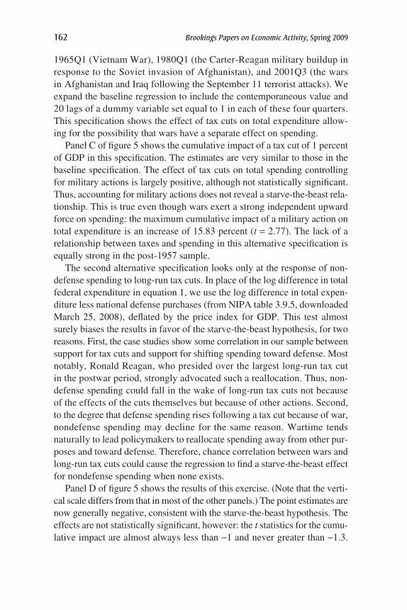
1965Q1 (Vietnam War), 1980Q1 (the Carter-Reagan military buildup inresponse to the Soviet invasion of Afghanistan), and 2001Q3 (the warsin Afghanistan and Iraq following the September 11 terrorist attacks). Weexpand the baseline regression to include the contemporaneous value and20 lags of a dummy variable set equal to 1 in each of these four quarters.This specification shows the effect of tax cuts on total expenditure allow-ing for the possibility that wars have a separate effect on spending.

Panel C of figure 5 shows the cumulative impact of a tax cut of 1 percentof GDP in this specification. The estimates are very similar to those in thebaseline specification. The effect of tax cuts on total spending controllingfor military actions is largely positive, although not statistically significant.Thus, accounting for military actions does not reveal a starve-the-beast rela-tionship. This is true even though wars exert a strong independent upwardforce on spending: the maximum cumulative impact of a military action ontotal expenditure is an increase of 15.83 percent (t = 2.77). The lack of arelationship between taxes and spending in this alternative specification isequally strong in the post-1957 sample.

The second alternative specification looks only at the response of non-defense spending to long-run tax cuts. In place of the log difference in totalfederal expenditure in equation 1, we use the log difference in total expen-diture less national defense purchases (from NIPA table 3.9.5, downloadedMarch 25, 2008), deflated by the price index for GDP. This test almostsurely biases the results in favor of the starve-the-beast hypothesis, for tworeasons. First, the case studies show some correlation in our sample betweensupport for tax cuts and support for shifting spending toward defense. Mostnotably, Ronald Reagan, who presided over the largest long-run tax cutin the postwar period, strongly advocated such a reallocation. Thus, non-defense spending could fall in the wake of long-run tax cuts not becauseof the effects of the cuts themselves but because of other actions. Second,to the degree that defense spending rises following a tax cut because of war,nondefense spending may decline for the same reason. Wartime tendsnaturally to lead policymakers to reallocate spending away from other pur-poses and toward defense. Therefore, chance correlation between wars andlong-run tax cuts could cause the regression to find a starve-the-beast effectfor nondefense spending when none exists.

Panel D of figure 5 shows the results of this exercise. (Note that the verti-cal scale differs from that in most of the other panels.) The point estimates arenow generally negative, consistent with the starve-the-beast hypothesis. Theeffects are not statistically significant, however: the t statistics for the cumu-lative impact are almost always less than −1 and never greater than −1.3.



More important, the estimates are small and not robust. Total expenditureless defense accounts, on average, for about 10 percent of GDP over oursample. Therefore, for a tax cut of 1 percent of GDP to reduce nondefensespending by the same amount, spending would need to decline by roughly10 percent. The estimated effect, however, is almost always a fall of lessthan 4 percent (or a rise). And dropping the Reagan tax cut (where, asdescribed above, an important omitted factor seems to have acted directlyto reduce nondefense spending) yields estimates that fluctuate irregularlyaround zero; similarly, either excluding the Korean War period or includ-ing the contemporaneous value and 20 lags of the dummy variable for mil-itary actions weakens the estimated effect considerably. Thus, there islittle evidence that tax cuts have a noticeable negative effect even on non-defense spending.

POLITICAL VARIABLES. A third robustness issue concerns the role of polit-ical variables. It is certainly possible that the party of the president or theexistence of unified government (that is, the same party controlling bothhouses of Congress and the presidency) has an influence on governmentspending. If such variables are correlated with our tax measure, the base-line regression could suffer from omitted variable bias. For this reason, wetry adding a variety of political variables to our baseline specification. Togive one example, panel E of figure 5 shows the effect of a tax cut on spend-ing when a dummy variable for Democratic administrations is included inthe regression. This regression asks whether tax cuts lower spending, tak-ing into account that Democratic presidents may consistently spend moreor less than their Republican counterparts. Adding this variable has verylittle effect on the estimates, although it strengthens the evidence for fiscalillusion or shared fiscal irresponsibility slightly: both the estimated posi-tive effects of tax cuts on spending and their statistical significance increasemodestly. We also consider specifications including a dummy variable forunified government, and including separate dummies for the first quarterof a new Republican or a new Democratic administration.15 Both specifica-tions change the estimates only trivially, and neither provides support forthe starve-the-beast hypothesis.

ALTERNATIVE TAX VARIABLE. A fourth concern involves the specification ofour tax variable. Our baseline series dates revenue changes in the quarterin which liabilities actually change. An alternative measure, which empha-sizes expectational effects, calculates the present discounted value of all


15. For the latter specification, we include both the contemporaneous value and 15 lagsof the new Republican and new Democratic dummy variables.


revenue changes called for by a given piece of legislation and dates the rev-enue change in the quarter the law was passed.16 Panel F of figure 5 showsthat the starve-the-beast hypothesis fares even worse when this alternativetax measure is used: the estimated impact of a tax cut on spending is gen-erally in the opposite direction from the prediction of the hypothesis, oftenlarge, and sometimes marginally significant.

ALTERNATIVE SPENDING CONCEPTS. Our baseline specification uses a NIPAmeasure of total spending on the grounds that it is available quarterly andis likely to correspond most closely with economic concepts of govern-ment spending. A natural alternative is to use the official budget numbers,which may be more closely tied to policymakers’ intentions. To do this,we aggregate our quarterly measure of long-run tax changes to constructa fiscal-year measure, and then reestimate equation 1 using the change inthe logarithm of the budget-based real expenditure measure and the con-temporaneous value and five annual lags of our tax measure.

For there to be a substantial starve-the-beast effect, tax cuts wouldalmost certainly have to reduce not just discretionary spending, but alsospending on entitlement programs. At the same time, because policy-makers can change discretionary spending more quickly, it is interestingto ask whether there is a starve-the-beast effect for this type of spend-ing. We therefore also examine the response of discretionary spendingto long-run tax cuts, again using annual budget data and five annual lagsof our tax measure.17

Panels G and H of figure 5 show the results. Once again, there is no sup-port for the starve-the-beast hypothesis. The response of overall spendingusing the official budget measure (panel G) is quite similar to that usingthe NIPA measure in panel A. And discretionary spending (panel H,again on a different scale) rises even more than overall spending follow-


16. See Romer and Romer (2009) for a detailed description of how we calculate thepresent value of revenue changes.

17. The budget data are from Budget of the United States Government: Historical TablesFiscal Year 2009 (www.gpoaccess.gov/usbudget/fy09/hist.html, tables 3.1 and 8.1, down-loaded March 16, 2009). We measure overall spending as total federal spending minus netinterest. Discretionary spending figures are available only beginning in 1962. For the years upthrough 1962, we estimate the growth rate of discretionary spending as the change in the logof total spending minus the sum of Social Security, income security, veterans benefits andservices, agriculture, commerce and housing credit, net interest, and undistributed offsettingreceipts. The estimates constructed in this way track the official estimates for the years imme-diately after 1962 quite well. In aggregating our measure of long-run tax changes to fiscal-year values, we omit the transition quarter (1976Q3). We deflate both the overall spendingmeasure and the discretionary measure by the price index for GDP.


ing a tax cut, with a maximum increase of 11.01 percent after four years(t = 2.23).

ALTERNATIVE SPECIFICATIONS OF THE SPENDING VARIABLE. A final robust-ness issue involves the appropriate way to enter the spending variable. Inall of the specifications discussed so far, we examine the response of thegrowth rate of real government expenditure to long-run tax changes. Thecumulative impact therefore shows the effect of a tax change on the levelof real expenditure. We feel this is the appropriate measure for testing thestarve-the-beast hypothesis: does a tax cut change the spending decisions ofpolicymakers? However, an alternative form of the hypothesis could be thata tax cut reduces expenditure as a percent of GDP. In this view, a tax cutcould lower the share of spending in GDP not by changing policymakers’spending decisions, but by changing output growth.

To test this alternative version, we reestimate equation 1 using two dif-ferent specifications of the dependent variable. The more sensible of thetwo expresses real total expenditure as a percent of trend real GDP (wheretrend real GDP is calculated using a conventional Hodrick-Prescott filter),and then uses the change in this variable as the dependent variable in equa-tion 1.18 Detrending real GDP is reasonable because, to the extent that a taxcut causes a temporary boom, it will inherently tend to reduce real expendi-ture as a percent of actual GDP in the short run. We do not believe that thisis the mechanism proponents of even the alternative form of the starve-the-beast hypothesis have in mind. However, as a further robustness check, wealso reestimate equation 1 using the change in the ratio of total real expen-diture to actual real GDP.

Panels I and J of figure 5 show the results of these two exercises. (Thesetwo panels are on a different scale than the others in figure 5 because the dependent variable is now a percent of GDP, not a percent of total expen-diture.) Panel I shows that the results using the change in spending as a shareof trend GDP are very similar to the results using the percentage change inspending. A tax cut of 1 percent of GDP generally raises the share of spend-ing in GDP. The estimated maximum effect is large (0.94 percent of GDP)but only marginally significant (t = 1.92). Thus, the results again fail to sup-port the starve-the-beast hypothesis, and provide moderate support for thealternative view of fiscal illusion or shared fiscal irresponsibility.


18. We again calculate real expenditure by dividing nominal expenditure by the price indexfor GDP. Real GDP is constructed by dividing nominal GDP by the same price index. We fita Hodrick-Prescott filter (λ = 1600) to log real GDP for the full sample (1947Q1–2007Q4).



Panel J shows that a tax cut does not even reduce spending as a share ofactual GDP. The estimated effects fluctuate irregularly around zero. Theestimates suggest a marginally significant starve-the-beast effect in a singlequarter (quarter 9), but they are more often positive than negative, and theestimated long-run effect is positive, small, and very far from significant.That this second specification fails to support the starve-the-beast hypoth-esis is quite surprising. As discussed in Romer and Romer (forthcoming),the short-run stimulatory effects of tax cuts on output are very strong. Yeteven this rapid growth of output is not enough to generate a systematic fallin expenditure as a share of GDP.

The robustness checks in this section yield two conclusions. First, andmore important, the lack of support for the starve-the-beast hypothesis isvery robust: with the possible exception of the examination of nondefensespending, which appears to be biased in favor of the starve-the-beast hypoth-esis and for which the results are mixed, none of the specifications weconsider provide evidence that tax cuts reduce government expenditure.Second, although we find evidence for the alternative view of fiscal illu-sion or shared fiscal irresponsibility, it is only modest. The point estimatesconsistently suggest that tax cuts raise government expenditure, but theyare only occasionally significantly different from zero, and then usuallyonly marginally so.

II.E. The Relationship between Other Types of Tax Changes and Total Expenditure

As discussed above, we focus on the response of government spendingto long-run tax changes because this is likely to provide the least biasedtest of the starve-the-beast hypothesis. Nevertheless, it is interesting to lookat the behavior of spending following the other types of tax changes we haveidentified: deficit-driven, countercyclical, and spending-driven. This analy-sis can reveal whether the feared biases from using these other types of taxchanges to estimate the response of spending appear to be present. It can alsoprovide an indirect check on our classification procedures. For example,if we have classified spending-driven tax changes correctly, they shouldbe positively correlated with spending changes.

For this exercise we reestimate equation 1 using the contemporaneousvalue and 20 lags of a particular type of tax change as the independent vari-able. We estimate a separate regression for each type of tax change, usingdata from the full postwar sample period. The results are again summarizedby calculating the implied cumulative response of spending to a tax cut (of agiven type) of 1 percent of GDP. Figure 6 presents the results for each type



of tax action.19 To facilitate comparisons, the first panel repeats our base-line results for long-run tax actions from figure 2.

DEFICIT-DRIVEN TAX CHANGES. Of the three additional types of tax changes,those driven by deficits are likely to be the most informative about thestarve-the-beast hypothesis. Like the long-run changes, these actions arenot taken in response to current or prospective short-run macroeconomicconditions or because spending is moving in the same direction. The reasonfor excluding these changes from the baseline regression was that deficit-driven tax increases are often parts of deficit reduction packages that includespending reductions. These observations might therefore bias the resultsagainst the starve-the-beast hypothesis. The estimated impact of deficit-driven tax changes on total expenditure (second panel of figure 6) shows thisfear is somewhat justified. In the quarter of a deficit-driven tax cut and thesubsequent two quarters, spending rises substantially. Or, to put it in terms ofthe realistic case, following a deficit-driven tax increase, spending falls sub-stantially. This is exactly the sort of inverse relationship one would expect ifdeficit reduction packages were common. The effects, although large, arenot precisely estimated. The t statistic for the maximum impact is 1.98.

After the first few quarters, the estimated effects of a deficit-driven taxcut turn negative for several years but return to positive at distant horizons.None of these estimates are close to statistically significant, however. Theseresults suggest that any spending cuts agreed to at the time of a deficit-driven tax increase disappear within the first year. The lack of a consistentpattern to the estimates at longer horizons suggests little ultimate impact oftax changes on expenditure. In this way, the results for deficit-driven taxchanges echo those for long-run actions and do not support the starve-the-beast hypothesis.

COUNTERCYCLICAL TAX CHANGES. The third panel of figure 6 shows theimplied impact on spending of a countercyclical tax cut. We exclude suchtax changes from our baseline regression because the state of the economycould tend to influence spending and taxes in opposite directions, and soagain bias the estimates against the starve-the-beast hypothesis. The resultssuggest that this is somewhat the case. A countercyclical tax cut is associatedwith a persistent rise in spending. However, the standard errors are quitelarge, so it is impossible to reject the hypothesis of no relationship.

19. This way of summarizing the estimates is slightly less intuitive for deficit-driven andspending-driven tax changes than for our baseline case of long-run changes, because deficit-and spending-driven tax changes are almost always tax increases. Nevertheless, the interpre-tation is the same as before: a negative response of spending to a tax cut is supportive of thestarve-the-beast hypothesis; a positive response or no response is not.




PercentLong-run tax changesa

2 4 6 8 10 12 14 16 18

–12

–6

0

6

12

–12

–6

0

6

12

–12

–6

0

6

12

PercentDeficit-driven tax changes

PercentCountercyclical tax changes



Figure 6. Cumulative Impact of a Tax Cut of 1 Percent of GDP on Total Expenditure,by Type of Tax Cut




PercentAll legislated tax changes

2 4 6 8 10 12 14 16 18

–12

–6

0

6

12

–12

–6

0

6

12

PercentAll legislated tax changes except spending-driven


Source: Authors’ regressions.a. Repeated from figure 2.

–12

–6

0

6

12

PercentSpending-driven tax changes


Figure 6. Cumulative Impact of a Tax Cut of 1 Percent of GDP on Total Expenditure,by Type of Tax Cut (Continued)


SPENDING-DRIVEN TAX CHANGES. The fourth panel of figure 6 shows thebehavior of government spending following a spending-driven tax cut. Inthis case the relationship is negative, large in absolute terms, and highlystatistically significant.20 This is exactly the result one would expect: if wehave classified spending-driven tax changes correctly, there should be a pos-itive correlation between them and spending. That the relationship persists isconsistent with the spending changes associated with these spending-drivenactions being permanent. The findings for spending-driven tax changesboth confirm our classification and illustrate the importance of controllingfor motivation when testing the starve-the-beast hypothesis. Includingspending-driven actions would clearly bias the results toward finding a pos-itive correlation between spending changes and tax changes.

ALL LEGISLATED TAX CHANGES. One way to see how much bias would resultfrom including spending-driven tax changes in our analysis is to definea tax variable that sums all four types of legislated tax changes and thenuse this as the explanatory variable in equation 1. The fifth panel of fig-ure 6 shows the implied impact on total expenditure of a legislated tax cutof any motivation of 1 percent of GDP. The estimated response is stronglynegative, and often statistically significant, for the first three years after atax cut. The point estimate for the maximum cumulative effect is −3.82 per-cent (t = −2.41). Since none of the other types of tax changes show a con-sistent negative response, this implied negative effect of the aggregate taxvariable must reflect the influence of the spending-driven tax changes.

To test this proposition more directly, we define a second composite taxvariable that includes all legislated tax changes other than those motivatedby spending changes. The last panel of figure 6 shows the cumulativeresponse of total expenditure to a non-spending-driven legislated tax cutof 1 percent of GDP. The effects are consistently positive, suggesting that,if anything, tax cuts appear to be followed by increases in governmentspending, not decreases as the starve-the-beast hypothesis predicts. And,for horizons beyond three years, these positive effects are significantly dif-ferent from zero.

THE CHANGE IN CYCLICALLY ADJUSTED REVENUE. These results suggest that theinclusion of spending-driven tax changes in the sample may explain whymuch of the previous literature has found evidence for the starve-the-beasthypothesis. This possibility can be investigated further by considering a


20. These findings are somewhat sensitive to the sample period. Some of the largestspending-driven tax changes occurred during the Korean War. When the post-1957 sampleperiod is used, the maximum impact of a spending-driven tax cut of 1 percent of GDP is large(−6.65 percent) but not statistically significant (t = −1.60).



21. For comparability with our tax measure, we use the change in real cyclically adjustedrevenue as a percent of real GDP. See Romer and Romer (forthcoming) for a more detaileddiscussion of the sources and derivation of this measure.


PercentAll changes in cyclically adjusted revenue

1 2 3 4 5 6 7 8 9 10

1 2 3 4 5 6 7 8 9 10

–12

–6

0

6

12

–12

–6

0

6

12

PercentAll changes in cyclically adjusted revenue except spending-driven


Source: Authors’ regressions.a. Based on regressions using revenue changes measured as the change in real cyclically adjusted

revenue as a percent of real GDP; the contemporaneous value and 11 lags are entered for the period1950Q1–2007Q4.

Figure 7. Cumulative Impact of a Tax Cut of 1 Percent of GDP on Total Expenditure,Estimates Using Cyclically Adjusted Revenuea

more standard measure of tax changes. A typical test of the starve-the-beasthypothesis uses the change in cyclically adjusted revenue, which includesall changes in revenue not related to short-run fluctuations in income, as themeasure of tax changes. Data on the change in cyclically adjusted revenueare available beginning in 1947Q2. We therefore investigate the effects ofusing the contemporaneous value and 11 lags of this variable as the taxmeasure for the period 1950Q1–2007Q4.21 When we use this conventionaltax variable, the results indeed seem to support the starve-the-beast hypo-thesis. The top panel of figure 7 shows that the estimated cumulative effect


of a decline in real cyclically adjusted revenue of 1 percent of GDP startsout positive but then turns negative. The maximum impact is a change ingovernment expenditure of −2.94 percent (t = −2.04).

If spending-driven tax changes are driving this result, subtracting thesechanges from the change in cyclically adjusted revenue should cause theeffect to disappear.22 Indeed, the results using such a series (bottom panel offigure 7) are dramatically different from those using the total change in cycli-cally adjusted revenue. The estimated impact of a 1-percent-of-GDP declinein cyclically adjusted revenue less spending-driven changes is stronglypositive in the short run: the maximum impact is 3.63 percent (t = 4.56).It then gradually declines toward zero, but it never turns negative over the11-quarter horizon we consider. Thus, the results provide no support forthe starve-the-beast hypothesis and, indeed, are somewhat supportive ofshared fiscal irresponsibility. This supports the view that the inclusion ofspending-driven changes in conventional revenue measures is an impor-tant source of the finding that government spending moves in the samedirection as tax revenue.23

III. Effects of Long-Run Tax Changes on Future Taxes

Our analysis finds no evidence that tax cuts lead to reductions in govern-ment spending. This finding naturally raises another question: how thendoes the government budget adjust to the cuts? An obvious possibility isthat the adjustment occurs on the tax side rather than on the expenditureside. To explore this possibility, we examine the response of both tax rev-enue and tax legislation to long-run tax changes.24


22. Since both series are expressed as a percent of GDP, the spending-driven tax changescan be subtracted without further adjustment.

23. The importance of spending-driven tax changes in biasing the results toward findinga starve-the-beast effect is sensitive to the sample period used. Spending-driven changes werelargest during the Korean War and tend to cause substantial bias in samples that include thisperiod. In later sample periods, spending-driven changes are smaller and so are a less impor-tant source of bias. This may explain why studies such as Ram (1988), Miller and Russek(1990), and Bohn (1991), which use data from the Korean War period and before, find sup-port for the starve-the-beast hypothesis, whereas those such as von Furstenberg, Green, andJeong (1986), which use data starting in 1954, do not.

24. Bohn (1991) also examines the degree to which deficits caused by falls in revenueare eliminated by subsequent tax increases. But because he does not account for the sourcesof changes in revenue, his estimates may suffer from important omitted variable bias. This isparticularly true because many of the most important revenue changes in his sample areassociated with wars.



III.A. Response of Tax Revenue

To investigate how revenue responds to long-run tax changes, we firstreestimate equation 1 using a measure of the change in real tax revenue asthe dependent variable. That is, we regress the percentage change in realrevenue on a constant and on the contemporaneous value and 20 lags ofour measure of long-run tax actions. As in the VARs in section II, wemeasure revenue using NIPA federal total receipts, deflated by the priceindex for GDP. We estimate the revenue response over both the full post-war sample period (1950Q1–2007Q4) and the post–Korean War sample(1957Q1–2007Q4).

The top and middle panels of figure 8 show the implied cumulativeresponse of total receipts to a long-run tax cut of 1 percent of GDP in eachsample period. Tax receipts decline strongly in the short run in response toa tax cut. The contemporaneous effect is a change in receipts of −1.90 per-cent in the full sample (t = −2.00) and −2.06 percent in the post–KoreanWar sample (t = −2.33). Total receipts remain substantially below theirpre–tax cut path for the next year and a half.

In both samples, receipts then recover substantially. For the full sample, the rise in revenue two years after the tax cut is dramatic andmarginally significant. This finding is largely driven by the KoreanWar. As described in section IV, the large 1948 tax cut was followedroughly two years later by the outbreak of the war. Three major taxincreases were passed during the war, and the war was accompanied by rapid output growth. For this reason the results for the full samplealmost surely overstate the true tendency of revenue to rebound. Forthe post–Korean War sample, receipts rise above their pre–tax cut pathseven quarters after the tax cut, but the effect is modest and the stan-dard errors are large (the t statistic for the positive effect does not riseabove 1).

To further investigate the response of receipts to tax shocks, we alsoestimate a bivariate VAR using our measure of long-run tax changes andthe log of real total receipts. We include 12 lags of each series, whichallows us to use our baseline sample period of 1950Q1–2007Q4. Thebottom panel of figure 8 shows the response of real receipts to a long-runtax cut of 1 percent of GDP in this specification. Receipts fall markedlyfollowing a long-run tax cut, and the effects are significant, or nearly so,for the first year and a half. Receipts then turn positive nine quarters afterthe shock. However, even though this specification uses the full sample,



–4

0

4

8


PercentOLS estimates, full sampleb

2 4 6 8 10 12 14 16 18

Source: Authors’ estimates.a. Based on regressions of the percentage change in real revenue (NIPA federal total receipts deflated

by the price index for GDP) on a constant and the contemporaneous value and 20 lags of the measure oflong-run tax changes.

b. Regression is estimated for the full postwar sample period (1950Q1–2007Q4).c. Regression is estimated for the post–Korean War sample period (1957Q1–2007Q4).d. Impulse response function from a VAR using the logarithm of real total receipts and the measure of

long-run tax changes estimated for the full postwar sample period; there are 12 lags, and the tax measureis ordered first.

–4

0

4

8


PercentOLS estimates, sample excluding Korean Warc

2 4 6 8 10 12 14 16 18

–4

0

4

8


PercentTwo-variable VAR, full sampled

4 8 12 16 20 24 28 32 36

Figure 8. Cumulative Impact of a Tax Cut of 1 Percent of GDP on Total Receiptsa



25. The response of total receipts to a long-run tax cut is even more negative whenthe bivariate VAR includes 20 lags of each variable and is estimated over the shortersample period 1952Q2–2007Q4. For this specification, tax revenue does not turn consis-tently positive until four years after the tax cut. The results for the behavior of revenueusing the multivariate VARs described in section II are broadly similar to those from the bivariate VAR. For example, in the four-variable VAR that includes our measure oflong-run tax changes, government expenditure, debt, and tax receipts, the effect of along-run tax change of 1 percent of GDP on receipts is negative for the contemporaneousquarter and the six quarters after the shock and then turns positive. The positive effectsare somewhat larger than in the bivariate VAR, but still small in absolute terms and notsignificant.

the positive effects are extremely small in absolute terms and not statisti-cally significant.25

III.B. Response of Tax Legislation

To understand the behavior of revenue following a long-run tax cut, it isimportant to investigate the behavior of subsequent tax legislation. Doestax revenue recover because of unusually rapid growth in the economy, orbecause policymakers legislate tax increases? Given that we have con-structed measures of the revenue impact of legislated tax changes classi-fied by motivation, this is an issue we can investigate.

In our single-equation analyses of spending and revenue, we considerthe experiment of a tax cut intended to spur long-run growth that is not fol-lowed by any additional tax changes based on long-run considerations.Therefore, it does not make sense to ask how long-run tax changes respondto this experiment. But it is reasonable to ask how other types of legislatedtax changes respond to a long-run tax cut. Long-run tax cuts that do notlower spending, and so increase the deficit, might lead to tax increasesdesigned to reduce an inherited budget deficit. Likewise, a long-run taxcut that gives rise to a short-run boom could lead to a countercyclical taxincrease. A long-run tax cut could also lead policymakers to switch to a“pay-as-you-go” policy: a budget deficit resulting from a long-run tax cutmay make policymakers unwilling to increase spending without increas-ing taxes. Therefore, one could also see an increase in spending-driventax increases following long-run tax cuts.

Our basic empirical framework is again identical to that in equation 1,except that the dependent variable is now a measure of legislated tax changes.That is, we regress legislated tax changes of some motivation on a constantand on the contemporaneous and lagged values of our measure of long-runtax changes. In our baseline specification we again use 20 lags, but we also



Percent of GDPOn deficit-driven tax changes

2

0

0.4

0.8

1.2

4 6 8 10 12 14 16 18


Percent of GDPOn countercyclical tax changes

2

0

0.4

0.8

1.2

4 6 8 10 12 14 16 18

Figure 9. Cumulative Impact of a Tax Cut of 1 Percent of GDP on Subsequent TaxChanges, by Typea


experiment with longer lags. We estimate the responses over both the fullpostwar sample and the post–Korean War sample. As before, we summarizethe results by examining the cumulative impact of a long-run tax cut of 1 per-cent of GDP. A positive impact implies that subsequent tax actions coun-teracted the long-run tax cut. Because the other tax variables are alsoexpressed as a percent of nominal GDP, the cumulative impact can beinterpreted as the fraction of the long-run tax cut that is undone over thehorizon considered.

Figure 9 shows the estimated impacts of a long-run tax cut of 1 percentof GDP on tax changes of various types. The first panel shows that theimpact on deficit-driven tax actions is positive and highly statistically signif-icant, suggesting that long-run tax cuts tend to be followed by deficit-driventax increases. The cumulative impact is 0.23 percentage point (t = 3.06) after



PercentOn spending-driven tax changes

2

0

0.4

0.8

1.2

4 6 8 10 12 14 16 18


PercentOn all three types

2

0

0.4

0.8

1.2

4 6 8 10 12 14 16 18

Source: Authors’ regressionsa. Based on regressions of the measure of legislated tax changes of the indicated type on a constant and

the contemporaneous and 20 lagged values of the measure of long-run tax changes. Estimates are for thefull postwar sample period (1950Q1–2007Q4).

Figure 9. Cumulative Impact of a Tax Cut of 1 Percent of GDP on Subsequent TaxChanges, by Typea (Continued)

8 quarters and 0.24 percentage point (t = 2.39) after 16 quarters.26 Thissuggests that about a fifth of a long-run tax cut is undone by deficit-driventax increases within a few years. These results are highly robust. Starting


26. The contemporaneous impact is substantial (0.11 percentage point; t = 3.73). Themost important observation behind this estimate is 1983Q1. A large part of the tax cuts in theEconomic Recovery Tax Act of 1981 were scheduled to go into effect in that quarter. Con-cern about current and prospective deficits, however, led to passage of the Tax Equity andFiscal Responsibility Act of 1982, which raised revenue mainly by modifying some featuresof the 1981 act that had already taken effect (Romer and Romer 2009). Thus, although thelong-run tax cut and the deficit-driven tax increase occurred simultaneously, there is a clearsense in which the deficit-driven increase was a response to the long-run cut.


the sample in 1957 has virtually no impact, and increasing the number oflags to 40 and carrying out the simulations for 10 years strengthen theresults. Ten years after the long-run tax action, 44 percent of the action hasbeen undone by deficit-driven tax increases (t = 2.53).

The second panel in figure 9 shows the impact of a long-run tax cuton countercyclical tax actions. The estimated impact is moderate but notclose to significantly different from zero. After 20 quarters, countercycli-cal tax actions have counteracted 18 percent of a long-run tax cut (t = 0.57).Starting the sample in 1957 has virtually no impact, because there were nocountercyclical tax actions in the early 1950s. Including more lags sug-gests that the response diminishes at longer horizons. The estimated effectafter 10 years is 0.11 percentage point (t = 0.21).27

The third panel of figure 9 shows the impact of a long-run tax cut onspending-driven tax changes. In this case the effects are virtually zero forthe first nine quarters and then turn strongly positive. The maximum cumu-lative impact is 0.47 percentage point (t = 2.53) after 14 quarters. Theimpact after 20 quarters is 0.36 percentage point (t = 1.58). This suggeststhat spending-driven tax increases occur after a long-run tax cut and thatthey counteract close to half of the initial cut. Thus, long-run tax cuts mayindeed tend to give rise to pay-as-you-go policies.

More than with the other tax changes, there is reason to be concernedthat the results for spending-driven actions are influenced by the observa-tions from the Korean War. Starting the sample in 1957 does indeed weakenthe link substantially. The strongest impact of a long-run tax cut is now arise in spending-driven taxes of 0.14 percentage point after eight quarters(t = 2.03). Likewise, including 40 lags reduces the impact substantially forthe full sample, but this effect is due entirely to the required shortening ofthe sample period.

The last panel of figure 9 shows the effect of a long-run tax cut on the otherthree types of legislated tax changes combined. The effect is positive, large,and significant: 0.61 percentage point (t = 2.08) after 12 quarters, 0.81 per-centage point (t = 2.34) after 16, and 0.74 percentage point (t = 1.92)after 20. This suggests that roughly three-quarters of a long-run tax cut is typ-ically undone by legislated tax increases of various sorts within five years.


27. We also experiment with leaving out the 1975 tax rebate, which is a huge outlieramong countercyclical actions, because it mainly cut taxes dramatically in one quarter andthen raised them dramatically in the next. Zeroing out this action reduces the response atmedium horizons but has almost no effect on the longer-run response. The main effect is tocut the standard errors by more than half.



Figure 10 reports the results of three robustness checks for the effect ofa long-run tax cut on this composite of other tax changes. The top panelshows the impact of starting the sample in 1957. Both the maximum impactand the statistical significance are somewhat reduced by this change. Theimpact now peaks at 0.60 percentage point (t = 1.66) after 19 quarters. Themiddle panel shows the effect of including 40 lags of long-run tax changes.The required shortening of the sample reduces the estimated response overthe first 20 quarters somewhat. Thereafter it moves irregularly upward. Theresponse after 40 quarters is large (0.77 percentage point) but not preciselyestimated (t = 1.39). Although they weaken the evidence slightly, these tworobustness checks tend to confirm that a large fraction of a long-run tax cutis typically reversed by legislated tax increases within the next few years.

Our final robustness check allows for more complicated dynamics. Weestimate a bivariate VAR that includes both our measure of long-run taxchanges and the composite measure of the three other types of legislatedtax changes. We include 12 lags of each series and estimate the VAR overour baseline sample period of 1950Q1–2007Q4.28

The bottom panel of figure 10 shows the response of other legislated taxchanges to a long-run tax cut of 1 percent of GDP in this specification. Theresults are again very similar to those from the single-equation specification.The response of other tax changes is strongly positive: the maximum effect is0.78 percentage point (t = 2.22) 18 quarters after the shock. The effect dimin-ishes slightly thereafter but levels off at around 0.65 percentage point. Thus,the VAR specification confirms that long-run tax cuts tend to be substantiallycounteracted by other types of tax increases over the next several years.

III.C. Discussion

The fact that policymakers have been able to largely reverse tax cuts helpsto explain why the cuts have not reduced spending.29 To see this connection,note that a tax cut could reduce future spending in either of two ways. Thefirst is through debt: by bequeathing greater debt to future policymakers,

28. The experiment we can consider in this framework is again slightly different fromthat in the single-equation specification. When we look at the effect of an innovation to long-run tax changes in the VAR specification, we are no longer assuming that the tax change isnot followed by other long-run tax changes. Rather, we let the data say how long-run taxchanges respond to the innovation. The cumulative response of long-run tax changes to along-run tax cut of 1 percent of GDP levels off at around −1.2 percentage points. This sug-gests that a long-run tax change is typically followed by subsequent long-run tax changesin the same direction. This is consistent with the fact that many long-run tax changes arelegislated to take effect in a series of steps.

29. We are grateful to our discussant Steven Davis for this point.



0

0.4

0.8

1.2


PercentSample excluding Korean War

2 4 6 8 10 12 14 16 18

0

0.4

0.8

1.2


PercentIncluding 40 lags of the tax change variable

4 8 12 16 20 24 28 32 36

0

0.4

0.8

1.2


PercentTwo-variable VAR estimatesb

4 8 12 16 20 24 28 32 36

Source: Authors’ estimates.a. Based on regressions of the measure of legislated tax changes of all types other than long-run tax

changes on a constant and the contemporaneous and lagged values of the measure of long-run tax changes. Regressions include 20 lags of the tax variable and are estimated for the full postwar sample except where indicated otherwise.

b. Impulse response function from a VAR using the measure of long-run tax changes and the composite measure of the three other types of legislated tax changes; there are 12 lags, and the long-run tax measure is ordered first.

Figure 10. Cumulative Impact of a Tax Cut of 1 Percent of GDP on Subsequent TaxChanges, Alternative Specificationsa


current policymakers restrict future policymakers’ choice set, which islikely to lead to some combination of higher taxes and lower spending. Thisis the mechanism emphasized in standard models of strategic budget deficits(for example, Tabellini and Alesina 1990 and Persson and Svensson 1989).The second is by leaving future policymakers with less tax revenue. Ifincreasing taxes is costly, this further reduces spending. This mechanismappears important in informal discussions of the starve-the-beast effect(see, for example, the quotation from Ronald Reagan at the beginning ofthe paper, which seems to suggest a permanent reduction in governmentrevenue).

If the costs of reversing a tax cut are small relative to the costs of cuttingspending, then only the first channel is relevant. And that channel is likelyto be quantitatively small. Suppose, for example, that a policymaker cutstaxes by 2 percent of GDP for five years. The result will be a deficit that islarger than it otherwise would have been by about 2 percent of GDP forfive years, and thus a stock of debt that is larger by about 10 percent ofGDP after five years. If the difference between the real interest rate andthe economy’s growth rate is 2 percentage points, then the interest costsassociated with maintaining the debt-to-GDP ratio at its higher level areabout 0.2 percent of GDP (2 percent times 10 percent). Thus, policy-makers can keep the tax cut from raising the debt-to-GDP ratio further byfirst undoing the tax cut and then enacting a permanent spending reduc-tion of 0.1 percent of GDP and an additional permanent tax increase of0.1 percent of GDP. Since spending is about 20 percent of GDP, this cor-responds to a spending reduction of about 0.5 percent—a quite small starve-the-beast effect.

If, however, undoing the tax cut is difficult, the effect is much stronger.In the extreme case where none of the tax cut can be reversed, satisfyingthe government budget constraint requires a spending cut equal to the taxcut (or by even more if there is a delay between the tax cut and the spend-ing reduction, so that the amount of debt increases before the spendingreduction). The result is a spending reduction of about 10 percent.

Our results concerning the behavior of tax legislation following tax cutssuggest that the truth is closer to the first case than to the second. This sug-gests a critical reason for our failure to find a substantial starve-the-beasteffect: adjustment on the tax side, although presumably not costless, appearsfeasible, making large adjustments on the spending side unnecessary.

We also find that the overall rebound in revenue exceeds the portiondue to legislated changes. The key source of the nonlegislated change inrevenue is almost certainly the effect of the tax cut on economic activity.



In Romer and Romer (forthcoming), we find that a tax cut of 1 percent ofGDP increases real output by approximately 3 percent over the next threeyears. Since revenue is a function of income, this growth raises revenue.

There is, however, an important caveat to this finding that tax cuts partlypay for themselves through more rapid growth: some of the output responseis almost surely a transitory departure of output from normal, not a perma-nent change in the economy’s normal level of output. To the extent that thisis the case, some of the rebound in revenue is also temporary. As a result,without further legislated changes, there may be some long-run budgetaryshortfall in the wake of the tax cut.

Because of these complications, our results do not allow us to describewith complete confidence how the government budget constraint adjusts fol-lowing a tax cut. What we can say is that we find no evidence of adjustmenton the spending side, and considerable evidence of substantial adjustmenton the tax side.

IV. Spending and Taxes in Four Key Episodes

In this section we examine the four episodes in our sample that stand out ashaving the largest long-run tax cuts. This examination serves several pur-poses. The first is to see whether the narrative record suggests that the taxcuts affected spending decisions. We examine the reasoning that policy-makers gave for their spending behavior, and so check whether tax cutsappear to have had an important effect on the decisionmaking process. Tokeep the narrative analysis manageable, we focus primarily on presidentialdocuments and statements.30 However, in cases where congressional viewsappear to be central, or at odds with those of the executive branch, we alsoexamine congressional documents.

The second purpose is to check whether our regression results reflectconsistent patterns in the data. Specifically, we look at the behavior of over-all spending and its two broad components, defense purchases and non-defense spending, in each episode. This allows us to investigate whether therelationships shown by the regressions appear in the key episodes.

Our third purpose is to examine whether any omitted variables or idio-syncratic shocks account for the failure of spending to fall after a tax cut.


30. The key presidential documents that we use are the Budget of the United States Gov-ernment (abbreviated as Budget in citations) and the Economic Report of the President (abbre-viated as Economic Report). Presidential speeches are identified by their title and date as givenin Woolley and Peters, The American Presidency Project (www.presidency.ucsb.edu).


We ask whether any unusual developments in the episodes had importantimpacts on spending. This analysis can suggest whether the regressionresults overstate (or understate) the evidence against the starve-the-beasthypothesis.

The final purpose is to address a similar set of issues concerning the taxside of the episodes. We look at what tax actions were taken following thetax cuts, and thus again check whether the regression results reflect con-sistent patterns. Perhaps more important, we examine the reasons policy-makers gave for those actions to see to what extent they appear to have beenresponses to the cuts. As with spending, we also check whether idiosyncraticfactors were an important determinant of tax changes in each episode.

IV.A. The Revenue Act of 1948

The Revenue Act of 1948 was passed over President Harry Truman’s vetoin April 1948. The bill was projected to reduce revenue by 1.9 percent ofGDP beginning in 1948Q2. The primary motivation for the cut was a desireto improve economic efficiency by reducing marginal tax rates.31

The tax cut was followed by a substantial reduction in revenue. Truman’sview, however, was that government spending should be determined by con-siderations other than the level of revenue and that tax policy should beadjusted accordingly. The 1950 Economic Report provides a clear statementof this belief:

In fields such as resource development, education, health, and social secu-rity, Government programs are essential elements of our economic strength.If we cut these programs below the requirements of an expanding economy,we should be weakening some of the most important factors which promotethat expansion. Furthermore, we must maintain our programs for nationalsecurity and international peace. . . .

Government revenue policy should take into account both the needs ofsound Government finance and the needs of an expanding economy. (p. 8)

Consistent with this view, Truman’s main response to the tax cut was topropose a counteracting tax increase. He argued, “In a period of highprosperity it is not sound public policy for the Government to operate ata deficit. . . . I am, therefore, recommending new tax legislation to raiserevenues by 4 billion dollars” (1950 Budget, p. M5). This increase wouldhave offset 80 percent of the 1948 cut.


31. Our descriptions in this section of the motivations for tax changes and our figures fortheir revenue effects are based on Romer and Romer (2009). The revenue estimates excludethe effects of retroactive features of the bills.


Nonetheless, the fall in revenue appears to have had a marginal effect onTruman’s spending policies. In the 1949 Midyear Economic Report of thePresident, he explained, “When I submitted my budget for the fiscal year1950 last January, the programs of expenditure that I then recommendedwere held to a minimum consistent with our basic needs in view of the infla-tionary strain upon materials and manpower then prevailing” (p. 7). SinceTruman viewed the budget deficit as contributing to inflationary pressures(see, for example, his Annual Message to the Congress on the State of theUnion, January 5, 1949, p. 3), this points to at least some effect of the taxcut on spending decisions.

After North Korea invaded South Korea on June 25, 1950, taxes and thedeficit essentially disappeared from Truman’s discussions of spending. Evenmore than it had been in peacetime, his view was that spending should bedetermined by the country’s needs, and taxes adjusted accordingly. Forexample, in his budget message of January 1951, Truman described thespending side of the budget and then stated, “I shall shortly recommend anincrease in tax revenues in the conviction that we must attain a balancedbudget to provide a sound financial basis for what may be an extended periodof very high defense expenditures” (1952 Budget, p. M6).

Finally, although Congress’s view of the tax cut was obviously very dif-ferent from Truman’s, Congress does not appear to have sought lower spend-ing than the president. For example, in August 1948 Truman reported thatalthough Congress had not appropriated the full amount he had requestedfor fiscal 1948 and 1949, this shortfall was offset by two factors: somespending had been authorized but not yet appropriated, and several piecesof legislation had been enacted that would require higher spending, but nospending had yet been authorized. As a result, he expected spending infiscal 1949 to be significantly higher than what he had requested in Janu-ary (“Statement by the President: The Midyear Review of the Budget,”August 15, 1948, p. 3). Thus, there is no evidence of a starve-the-beasteffect operating through congressional actions in this episode.

The first panel of figure 11 shows the behavior of real government spend-ing in this episode. It plots, in logarithms, both our measure of total expen-diture and the two categories of spending, national defense purchasesand nondefense spending. As in section II, we define nondefense spendingas the difference between our measure of total expenditure and nationaldefense purchases; the two main components of this measure are non-defense purchases and current transfer payments. The vertical line indicatesthe quarter in which the tax cut took effect. Several things are apparent.First and most important, there was no discernable slowdown in overall




spending or in either of the two categories of spending. Indeed, growth inoverall spending increased after the tax cut. Total expenditure, which hadbeen essentially flat before the tax cut, rose by 16 percent (calculated usingthe change in logarithms) in the two years between the cut and the start of thewar. Second, there was a substantial one-time spike in nondefense spend-ing in 1950Q1, reflecting a one-time dividend payment from the trust fundfor National Service Life Insurance (the government insurance program formilitary personnel). These payments were the result of a large accumulationof assets in the trust fund, which could not be used for other purposes(Hines 1943; Survey of Current Business, March 1950, pp. 1–3, and August1950, p. 7). Third, both defense and overall spending rose sharply after theoutbreak of the war.

Both the National Service Life Insurance dividend payment and theincreased military spending after the start of the war clearly reflected unusualdevelopments, not just the normal response of spending to tax cuts. Thus,they tend to cause our regressions to overstate the impact of tax cuts onsubsequent spending increases.

Another important unusual development operated in the opposite direc-tion. The Social Security Amendments of 1950 almost doubled Social Secu-rity benefits starting in September 1950 and substantially increased thecoverage of the system beginning in January 1951 (Social Security Bulletin,October 1950, pp. 3–14). Because Social Security benefits were initiallysmall, these changes had little immediate impact on overall spending. None-theless, the rise in the benefit base and the expansion of coverage contributedsignificantly to the growth of spending over time. The fact that these delayedspending effects are not captured by our regressions tends to make themunderstate the impact of tax cuts on later spending increases.

On the tax side, the 1948 tax cut was followed by a series of tax increasesthat were largely spending driven. The first, and least important, was anincrease in Social Security taxes of 0.3 percent of GDP in 1950Q1, which hadbeen legislated before the tax cut was passed. Larger tax actions followed.The Social Security Amendments of 1950 increased the base of the payrolltax from $3,000 to $3,600, effective at the beginning of 1951, and called fora gradual increase in the combined (employer plus employee) Social Securitytax rate from 3 percent to 61⁄2 percent over the next two decades (Social Secu-rity Bulletin, October 1950, pp. 3–14). And three bills in 1950 and 1951 tofinance the Korean War increased taxes by a combined 4.1 percent of GDP.32

32. We measure the effect of a series of tax changes by finding the share of each one innominal GDP in the quarter in which it took place, and then summing the shares.


The move to spending-driven tax increases in the early 1950s was clearlya policy decision. In the case of Social Security, policymakers were grappling with how to finance the system. A special congressional com-mission and the Social Security Administration both recommended that Social Security taxes be limited and that the system move towardincreasing reliance on general revenue. Instead, however, the 1950amendments repealed the provision of the Social Security Act that permitted financing from general revenue, and made the system entirelyself-financing (Social Security Bulletin, May 1948, pp. 21–28; Feb-ruary 1949, pp. 3–9; October 1950, pp. 3–14). However, we have foundno direct evidence that the 1948 tax cut played a causal role in this decision.

The extent of the government’s reliance on contemporaneous tax increasesto finance the Korean War is remarkable: total government expenditure roseby 6.0 percent of GDP from 1950Q2 to its peak in 1952Q3, only moder-ately more than the expected revenue effects of the tax increases to financethe war. Moreover, Truman explicitly cited the deficit as a reason for


LogarithmsRevenue Act of 1948

0.5

1.0

1.5 Total expenditures

Tax cut takes effect


National defense purchasesNondefense spending

LogarithmsRevenue Act of 1964

1962

0.5

1.0

1.5

2.0

1963 1964 1965 1966 1967 1968

2.0

1953195219511950194919481947

Figure 11. Real Expenditure Following Major Long-Run Tax Cuts


this heavy reliance on tax finance. Soon after the war began, he wrote tocongressional leaders:

We embark on these enlarged expenditures at a time when the Federal budgetis already out of balance. This makes it imperative that we increase tax rev-enues promptly lest a growing deficit create new inflationary forces detri-mental to our defense effort.

We must make every effort to finance the greatest possible amount ofneeded expenditures by taxation. (“Letter to the Chairman, Senate Committeeon Finance, on the Need for an Increase in Taxes,” July 25, 1950, p. 1)

Thus, the Korean War tax increases were in part a response to the 1948tax cut.

IV.B. The Revenue Act of 1964

In February 1964 President Lyndon Johnson signed the Revenue Actof 1964. The act reduced revenue by 1.3 percent of GDP in 1964Q2 and by


Source: Authors’ calculations using National Income and Product Accounts data. a. The first vertical line marks the date of the Economic Growth and Tax Relief Reconciliation Act of

2001, and the second that of the Jobs and Growth Tax Relief Reconciliation Act of 2003.

Tax cuts take effect


LogarithmsEconomic Recovery Tax Act of 1981

1980

1.0

1.5

2.0

2.5

1981 1982 1983 1984 1985

LogarithmsTax cuts of 2001 and 2003a

2000 2001 2002 2003 2004 2005

1.5

2.0

2.5

3.0

Figure 11. Real Expenditure Following Major Long-Run Tax Cuts (Continued)


another 0.6 percent in 1965Q1. The key motivation for the tax cut was adesire to increase long-run growth.

Because economic growth following the tax cut was very rapid, rev-enue recovered quickly, and budget deficits that could have triggered astarve-the-beast response did not emerge immediately. Nevertheless, pol-icymakers’ statements and behavior provide some evidence concerningthis mechanism.

At almost the same time that he signed the tax bill, Johnson began topropose drastic increases in spending. In February 1964 he gave a speechproposing federal hospital insurance for the elderly and other health ini-tiatives (“Special Message to the Congress on the Nation’s Health,” Feb-ruary 10, 1964). His “Great Society” speech followed in May 1964, callingfor the elimination of poverty, urban renewal, pollution reduction, andexpansion of education (“Remarks at the University of Michigan,” May 22,1964). Over the next year, a number of spending increases directed atachieving these goals were passed. The most significant were the dramaticexpansion of benefits and the introduction of Medicare contained in theSocial Security Amendments of 1965.

The Johnson administration believed that spending should be determinedby necessity and efficiency. For example, the 1967 Economic Report stated,“most economists now agree that the selection of appropriate expenditurelevels . . . should be made in light of the relative merits of alternative pro-grams, and of the benefits of added public expenditures, compared withprivate ones, at the margin. . . . It is preferable to emphasize changes in taxrates (suitably coordinated with changes in monetary policy) for stabi-lization purposes” (p. 68). The narrative record in this episode is strikingin the degree to which revenue was not mentioned as a determinant ofexpenditure.

Defense spending increased substantially starting in mid-1965 because ofthe escalation of the war in Vietnam. Johnson argued forcefully againstallowing budgetary concerns to stop the rise in nondefense spending, stating:

There are men who cry out: We must sacrifice. Well, let us rather ask them:Who will they sacrifice? Are they going to sacrifice the children who seekthe learning, or the sick who need medical care, or the families who dwellin squalor now brightened by the hope of home? . . .

I believe that we can continue the Great Society while we fight in Viet-nam. (“Annual Message to the Congress on the State of the Union,” Janu-ary 12, 1966, p. 2)

Congress went along with his calls for increased spending. For example,the Social Security Amendments of 1967 brought about another substan-



tial increase in benefits and a significant increase in coverage. Thus, the risein spending following the tax cut was not just the consequence of the war.

Beginning in early 1966, policymakers began to worry that the economywas overheating, and by late that year the budget deficit had increased sub-stantially. Nevertheless, the administration did not call for substantial spend-ing reductions. Federal expenditure was expected to rise by $15 billion in1968 (1968 Economic Report, p. 54). Instead, the administration concludedthat “the cost of meeting our most pressing defense and civilian require-ments cannot be responsibly financed without a temporary tax increase”(1969 Budget, p. 8).

Over the president’s objection, Congress included a $6 billion spend-ing reduction (relative to projections) in the 1968 bill imposing a 10 per-cent temporary tax surcharge. Congress pressed for the spending cutsnot because revenue had declined, but because members felt it was unfairto take all of the needed macroeconomic restraint in the form of highertaxes. A number of senators expressed sentiments similar to those of Sena-tor Robert Byrd of West Virginia, who stated, “Before any new tax bur-den . . . is placed upon the American taxpayer, the executive branch andthe legislative branch should reduce, and eliminate where possible, allnonessential expenditures” (Congressional Record, 90th Congress, 2dsession, volume 114, part 7, April 2, 1968, p. 8561). The tax cut was surelyone factor contributing to the overheating that motivated the tax surcharge.Therefore, although policymakers did not explicitly draw a direct linkbetween the tax cut and the spending reduction, the reduction is the onedevelopment in this episode that could suggest some connection betweentax cuts and subsequent spending decisions.

The actual behavior of spending following the 1964 tax cut is completelyconsistent with policymakers’ stated positions. The second panel of figure 11shows that total expenditure was basically constant during the first yearafter the tax cut but then rose strongly. Total expenditure increased by27 percent in the five years after the tax cut, noticeably more than the 18 per-cent in the five years before the cut.33 The rise in defense purchases was onesource of the increase, but nondefense spending, fueled by a large increasein transfer payments, increased even more rapidly.

Special factors clearly played a role in the behavior of spending. Much ofthe rise in defense expenditure was related to the Vietnam War. To the extent


33. These changes are computed as the change (in logarithms) of our measure of realtotal gross expenditure less interest over the periods 1959Q2–1964Q2 and 1964Q2–1969Q2.The other figures for spending growth reported in this section are computed similarly.


that defense spending truly was nondiscretionary, some of the rise in spend-ing reflects this exogenous shock rather than a failure of the starve-the-beastphenomenon. At the same time, the immediate increase in spending calledfor by the Social Security Amendments of 1965 and 1967 understates in afundamental way the true rise in spending. The creation of the Medicareprogram and the increases in Social Security benefits and coverage put inplace an enormous stream of future spending. Thus, in present value terms,the increase in spending passed in the wake of the 1964 tax cut was unques-tionably huge.

Policymakers’ statements and actions on taxes in this episode are strik-ing. In 1965 the Johnson administration proposed (and succeeded in pass-ing) two significant tax actions. One was the Excise Tax Reduction Actof 1965, passed in January of that year. The administration viewed thistax cut as a continuation of the 1964 action. In this case, then, the serialcorrelation of tax changes reflects continuity in views about appropriatepolicy. The second was the Social Security Amendments of 1965, whichincluded a substantial increase in payroll taxes to help pay for a largeincrease in benefits, including hospital insurance for the elderly. Thistax increase appears to have had little to do with the 1964 tax cut. Policy-makers paid for the desired expansion of benefits by raising taxes, becausethe decision had been made in 1950 that the Social Security system shouldbe self-financing.34

The overheating of the economy beginning in 1966 led policymakersto advocate tax increases. The Tax Adjustment Act of 1966 (enacted inMarch) rescinded the excise tax reduction of the previous January, andPublic Law 89-800 (enacted in November) suspended the investment taxcredit. Together these two tax increases were expected to raise revenue by0.3 percent of GDP.35

By far the largest tax increase in the immediate post-1964 period wasthe 1968 surcharge. The administration first proposed a 6 percent surchargein January 1967. In August 1967 Johnson stated, “If left untended, thisdeficit could cause . . . a spiral of ruinous inflation” and “brutally higherinterest rates” (“Special Message to the Congress: The State of the Budget


34. The Social Security Amendments of 1967, enacted in January 1968, also raised taxessubstantially to pay for another increase in benefits and coverage.

35. Public Law 90-26, enacted in June 1967, restored the investment tax credit. As dis-cussed in Romer and Romer (2009), the motivation for this change involved the conditionsin a particular sector (the capital goods market) and concern about longer-run incentives forinvestment. It does not appear to have been motivated by the 1964 tax cut or by short-runmacroeconomic conditions.


and the Economy,” August 3, 1967, p. 1). He requested that the surchargebe increased to 10 percent, the level ultimately included in the Revenueand Expenditure Control Act of 1968. The act increased taxes by 0.9 per-cent of GDP in 1968Q3 and by another 0.2 percent in 1969Q1. Johnsonwas explicit in saying that the surcharge was undoing part of the 1964 taxcut. In his signing statement he said, “This temporary surcharge will returnto the Treasury about half the tax cuts I signed into law in 1964 and 1965”(June 28, 1968, p. 1). This action, combined with the continued rise inexpenditure, is a vivid example that what typically gives in response to atax cut is not spending but the tax cut itself.

IV.C. The Economic Recovery Tax Act of 1981

A very large long-run tax cut was enacted in August 1981, shortly afterPresident Ronald Reagan took office. The cut lowered taxes by a combined4.5 percent of GDP in a series of steps.

Reagan was a strong advocate of spending reductions throughout hispresidency. For example, in a speech presenting his economic program,he identified “reducing the growth in government spending and taxing” as acentral goal, and he argued that “spending by government must be limitedto those functions which are the proper province of government” (“Addressbefore a Joint Session of the Congress on the Program for Economic Recov-ery,” February 18, 1981, pp. 1, 5). Similarly, in his first budget message, inFebruary 1982, he listed “reducing the growth of overall Federal spendingby eliminating Federal activities that overstep the proper sphere of FederalGovernment responsibilities” as one of his fundamental economic goals(1983 Budget, p. M4).

The 1981 tax cut was followed by a substantial fall in revenue and asharp rise in the deficit. As the deficit increased, Reagan often cited it asa further reason for restraining spending. For example, in his February1986 budget message, he said, “there is a major threat looming on the hori-zon: the Federal deficit” (1987 Budget, p. M-4). He went on to say, “Spend-ing is the problem—not taxes—and spending must be cut. The programof spending cuts and other reforms contained in my budget will lead to abalanced budget at the end of five years” (p. M-5). Similarly, his February1988 budget message stated:

Last year, members of my Administration worked with the Leaders of Con-gress to develop a 2-year plan of deficit reduction—the Bipartisan BudgetAgreement. . . .

The Bipartisan Budget Agreement reflects give and take on all sides. Iagreed to some $29 billion in additional revenues and $13 billion less than



I had requested in defense funding over 2 years. However, because of awillingness of all sides to compromise, an agreement was reached thatpared $30 billion from the deficit projected for 1988 and $46 billion fromthat projected for 1989. (1989 Budget, p. 1-6)

Thus, the narrative record from this episode provides some evidence that thedecline in revenue due to the 1981 tax cut affected later spending decisions.

The third panel of figure 11 plots government spending before and afterthe 1981 tax cut. The vertical line is drawn at 1981Q3, the date of the firstof the series of cuts. Despite what the narrative evidence suggests, growthin overall spending did not slow but actually quickened. In the five yearsfollowing the tax cut, total expenditure grew by 23 percent, substantiallyabove the 14 percent growth in the five years before the cut. This accel-eration in overall spending reflects a combination of a large rise in thegrowth of defense spending and a more moderate rise in the growth of non-defense spending.

Two important unusual spending developments marked this episode.First, the tax cuts coincided with a shift in political power toward support-ers of lower spending. Reagan’s goal of restraining government spendingwas not shared by his predecessor. For example, in his final budget mes-sage, President Jimmy Carter, while advocating “budget restraint,” stated,“The growth of budget outlays is puzzling to many Americans, but itarises from valid social and national security concerns” (1982 Budget,pp. M4–M5). The balance of political power in Congress also swung sharplytoward advocates of spending restraint at the time of Reagan’s election.Thus, there was clearly an omitted variable acting to reduce spending inthis episode.36

Second, the heightening of the cold war prompted policymakers toincrease defense spending. Ramey and Shapiro (1998), for example, iden-tify the Soviet invasion of Afghanistan at the end of 1979 as an exogenouspositive shock to defense spending. This factor operated in the oppositedirection of the political shift toward supporters of lower spending.

The tax cuts were followed by two types of tax increases. First, the SocialSecurity Amendments of 1983 called for a series of payroll tax increasesfrom 1984 to 1990 to improve the solvency of the Social Security system.These increases appear to have been largely a continuing consequence ofthe 1950 decision to make the Social Security program self-financing.


36. Although Reagan supported spending reduction in general, he favored higher defensespending. He had campaigned on a need to rebuild the military and identified “strengtheningthe Nation’s defenses” as one of his key goals (1983 Budget, p. M4).


Second, a series of income tax increases were explicitly motivated bya desire to reduce the budget deficits that emerged following the tax cuts.These included the Tax Equity and Fiscal Responsibility Act of 1982, whichundid some of the provisions of the 1981 act; the Deficit Reduction Act of1984; the Omnibus Budget Reconciliation Act of 1987; and the OmnibusBudget Reconciliation Act of 1990. For example, in a national address onthe 1982 act, Reagan stated that it reflected a choice to “reduce deficits andinterest rates by raising revenue from those who are not now paying theirfair share,” rather than to “accept bigger budget deficits, higher interestrates, and higher unemployment” (“Address to the Nation on Federal Taxand Budget Reconciliation Legislation,” August 16, 1982, p. 4). Similarly,the 1989 Budget reported that the 1987 act was enacted “in conformancewith the Bipartisan Budget Agreement” (p. 4-5), which, as described above,was motivated by concern about the deficit. The 1982 and 1984 actionsalone increased taxes by 1.0 percent of GDP. Thus, these tax increaseswere a fairly direct response to the earlier tax cut.

IV.D. The Tax Cuts of 2001 and 2003

Two long-run tax cuts were passed early in the administration of Presi-dent George W. Bush. The Economic Growth and Tax Relief ReconciliationAct of 2001, enacted in June, included a long-run tax cut of 0.8 percent ofGDP in 2002Q1, as well as a large countercyclical tax cut in 2001Q3. TheJobs and Growth Tax Relief Reconciliation Act of 2003, enacted in May,included a long-run cut of 1.1 percent of GDP in 2003Q3.

These tax cuts do not appear to have had any substantial impact on theadministration’s view of appropriate spending. Throughout the episode, bothspending restraint and either preserving the surplus or reducing the deficitreceived some attention. But discussions of spending did not change appre-ciably in response either to the tax cuts or to the subsequent deteriorationof the budget situation.

The administration’s first budget proposals, which predated the tax cuts,put some emphasis on spending restraint and on paying down the nationaldebt. The president’s first budget document, for example, stated that thebudget would “Moderate Growth in Government and Fund National Prior-ities” and achieve “Debt Reduction” (“A Blueprint for New Beginnings: AResponsible Budget for America’s Priorities,” February 28, 2001, p. 7).37


37. This document was not part of the president’s formal 2002 budget, which was notsubmitted until April 2001. However, it is included with the other 2002 budget documents onthe Government Printing Office website. See www.gpoaccess.gov/usbudget/fy02/index.html.


It also said that “the President’s Budget commits to using today’s surplusesto reduce the Federal Government’s publicly held debt so that future gen-erations are not shackled with the responsibility of paying for the currentgeneration’s overspending” (p. 22), and that “we must ensure that we reinin excessive Government spending” (p. 23).

In the immediate aftermath of the terrorist attacks of September 11,2001, discussions of budget policy placed less emphasis on spendingrestraint (see, for example, Bush’s “Address before a Joint Session of theCongress on the State of the Union,” January 29, 2002, pp. 3–4). Laterpresidential statements, however, returned to calls for spending restraintsimilar to those in 2001. For example, in his 2004 State of the UnionAddress, Bush stated, “I will send you a budget that funds the war, protectsthe homeland, and meets important domestic needs while limiting thegrowth in discretionary spending. . . . By doing so, we can cut the deficit inhalf over the next 5 years” (“Address before a Joint Session of the Con-gress on the State of the Union,” January 20, 2004, p. 4). Similarly, in his2007 State of the Union Address, Bush said, “What we need is spendingdiscipline. . . . I will submit a budget that eliminates the Federal deficitwithin the next 5 years” (“Address before a Joint Session of the Congresson the State of the Union,” January 23, 2007, p. 1). Although these state-ments were very similar to those Bush had made before the tax cuts, actualbudget conditions had changed substantially: revenue had fallen and theoverall budget had shifted from surplus to deficit. The similarity in therhetoric despite the large changes in the deficit suggests that there waslittle link between the level of revenue and the perceived need for spend-ing restraint.

The last panel of figure 11 plots the major categories of spending inthis episode. The two vertical lines show the dates that the two tax cutsfirst took effect. As in the other episodes, overall spending growth didnot slow. In the five years following the first cut in 2001Q3, spending grewby 22 percent, substantially more than the 14 percent in the five yearsbefore the cut. The growth in spending following the tax cut was greatestin defense: national defense purchases rose by 33 percent in the five yearsafter the tax cut, while nondefense spending rose by 19 percent.

The events of September 11, 2001, were clearly an important outsideinfluence on spending. Some of the behavior of total expenditure surelyreflects the impact of this development rather than the effect of the taxcuts. On the other hand, one important spending action is not well reflectedin our spending measures. The addition of prescription drug coverage to



Medicare, enacted in December 2003, was expected to have only a modestshort-run effect on spending but to raise its path substantially over time.Thus, although the change was enacted soon after the tax cuts, most of itsimpact on spending will almost surely come after the period considered inour regressions.

One notable feature of this episode is that the tax cuts were not soonfollowed by counteracting tax increases. A modest countercyclical tax cutwas enacted in March 2002, in the wake of the September 11 attacks. Theonly important tax increase was that the bonus depreciation provisionsincluded in the 2002 bill, and then expanded and slightly extended as partof the 2003 tax bill, were allowed to expire at the end of 2004. Thus, theissue of how the government will eventually deal with the loss of revenuefrom the 2001 and 2003 tax cuts remains open.

IV.E. Assessment

Examination of these four episodes of major long-run tax cuts reinforcesthe findings from our statistical analysis: there is little evidence of a starve-the-beast effect. The one aspect of the episodes that is at times consistentwith the hypothesis that tax cuts reduce government spending is the narrativerecord of the budget process. Although the presidents in two of the episodes(Johnson and Bush) appear to have paid little attention to the impact of thetax cuts on revenue in formulating their budget policies, the presidents inthe other two (Truman and Reagan) cited the level of revenue as a consid-eration in budget policy. Even in these cases, however, other factors wereclearly much more important, and to a considerable extent the concernover revenue led not to advocacy of spending reductions, but to support for(or acceptance of) tax increases.

The actual behavior of spending in all four episodes provides no supportfor the starve-the-beast hypothesis. In no episode was there a discernibleslowdown in spending following the tax cut. Indeed, all of the episodes sawan acceleration of spending. This is similar to the overall statistical find-ing of a positive (although only marginally significant) effect of tax cuts onspending, and it suggests that the regression results reflect a consistent pat-tern in the data rather than the effects of outliers.

Examination of other influences on spending in the episodes does notchange these conclusions. On the one hand, there was an important exter-nal development in each episode that acted to raise defense spending. Byitself, this pattern would suggest that the regressions might overestimatethe positive effects of tax cuts on spending. Two considerations, however,



point in the opposite direction.38 First, the largest of the tax cuts (that of1981) coincided with the election of a president who had a strong commit-ment to reducing the size of government. This suggests that the positiveimpact of tax cuts on spending might be even larger than implied by theregressions. Second, significant actions were taken in three of the fourepisodes to increase spending that had important effects after the five-yearwindow considered in our baseline regressions. For example, in two of theepisodes (1964 and 2001–03), the government enacted major changes inthe provision of medical care for the elderly that had very large implica-tions for the long-term path of government spending. Since our regressionsmiss much of the effects of these actions, this too suggests that the regres-sions may underestimate the extent to which tax cuts increase spending.Thus, examination of other factors affecting spending in the four episodessuggests that, on net, the regressions do not overstate the evidence againstthe starve-the-beast hypothesis.

Tax policy in these episodes is also consistent with the regression results.In three of the four episodes, substantial tax increases followed the initialtax cut within five years, offsetting a substantial fraction of it. Perhapsmore striking is what policymakers said about the tax increases. In all threecases they referred directly to the need to raise taxes to counter the macro-economic and budgetary effects of the original tax cuts. And in two cases(1948 and 1964), the president said explicitly that raising taxes was prefer-able to cutting spending.

V. Conclusions

The starve-the-beast hypothesis—the idea that tax cuts restrain govern-ment spending—is a central argument for tax reduction. Despite its impor-tance, however, the hypothesis has been subject to few tests, and the teststhat have been done have important limitations.

This paper tests the starve-the-beast hypothesis by examining the behav-ior of government spending following tax changes motivated by long-runconsiderations. Because these tax changes were not motivated by factorsthat are likely to have an important direct effect on government spending,they are the most appropriate for testing the theory. The results provide noevidence of a starve-the-beast effect: following long-run tax cuts, govern-


38. In addition, recall that our statistical results are robust to controlling for a measure ofexogenous shocks to defense spending, and that even excluding defense spending entirelyprovides little evidence for the starve-the-beast hypothesis.


ment spending does not fall. Indeed, if anything, spending rises, providingsome support for the alternative view of fiscal illusion or shared fiscal irre-sponsibility. The lack of support for a starve-the-beast effect is highly robust.Detailed examination of the four largest postwar episodes of long-run taxcuts reinforces the statistical findings.

We also identify a potentially powerful source of bias in tests of thestarve-the-beast hypothesis that use data on overall revenue and spending.Some tax changes are explicitly motivated by contemporaneous or plannedchanges in spending. Not surprisingly, these tax changes are followed bylarge spending changes in the same direction. Causation in these cases, how-ever, runs from the decision to raise spending to the tax change. For the fullpostwar sample, this type of tax change is sufficiently common that it causesthe overall relationship between tax revenue and spending to be significantlypositive. Excluding these spending-driven changes makes the relationshipnegative and marginally significant.

The fact that tax cuts do not lead to spending reductions raises thequestion of how the government budget constraint is ultimately satisfied.We find that long-run tax cuts are offset by legislated and nonlegislated taxincreases over the next several years. The fact that policymakers are ableto make changes on the tax side helps to explain why they do not appear tomake large changes on the spending side.

Of course, failing to find support for the starve-the-beast hypothesisis not the same as definitively refuting it. There are several ways in whichour results are not inconsistent with the presence of at least some starve-the-beast effect. First, our failure to find such an effect for the postwar U.S.federal government does not mean it is not important in other times andplaces. Second, the case that focusing on tax changes taken for long-runpurposes yields unbiased estimates is not airtight. As we explain, how-ever, the most likely direction of bias is in favor of the starve-the-beasthypothesis, not against it. Third, because our estimates are not highlyprecise, the hypothesis that tax cuts exert some restraining influence onspending usually cannot be rejected. Fourth, some of our evidence (thestatistical examination of nondefense spending and the narrative evi-dence for the 1948 and 1981 episodes) provides some hints of support fora small starve-the-beast effect.

Finally, although we find that the fall in revenue caused by a tax cut dis-appears after a few years, some of this disappearance is most likely the resultof a temporary output boom. Thus, we do not completely resolve the issueof how the government restores long-run budget balance. Since the gov-ernment’s long-run budgetary situation deteriorated substantially over the



period we consider, to some extent this limitation is inherent: not all of theoffsetting actions have yet occurred. It is possible that some of the remain-ing adjustment will take place on the spending side.

Taken together, these caveats imply that one cannot necessarily con-clude that tax cuts do not restrain government spending at all. But it remainsthe case that, over the period we consider, there is virtually no evidence ofsuch an effect.

The finding that tax cuts do not appear to substantially restrain gov-ernment spending could obviously have implications for policy. At thevery least, policymakers should be aware that the historical experiencesuggests that tax cuts tend to lead to tax increases rather than to spend-ing cuts.

The finding also has implications for models that assume the existence ofa starve-the-beast effect. For example, Bohn (1992) argues that one reasonfor Ricardian equivalence to fail is that a tax cut implies that governmentspending will be lower; as a result, a tax cut leads households to reduce theirestimates of the present value of their present and future liabilities, and so toincrease their consumption. Similarly, a restraining effect of tax cuts on gov-ernment spending plays a central role in the theories of strategic debt accu-mulation of Torsten Persson and Lars Svensson (1989), Guido Tabellini andAlberto Alesina (1990), and others. If decisionmakers understand that taxcuts do not in fact lead to substantial reductions in government spending,these mechanisms are much less important. Thus, better estimates of theeffects of tax cuts on spending may require changes to the modeling of awide range of issues.

ACKNOWLEDGMENTS We are grateful to Alan Auerbach, Raj Chetty,Steven Davis, Barry Eichengreen, William Gale, Jeffrey Miron, and Ivo Welchfor helpful comments and suggestions, and to the National Science Foundationfor financial support.



References

Anderson, William, Myles S. Wallace, and John T. Warner. 1986. “GovernmentSpending and Taxation: What Causes What?” Southern Economic Journal 52,no. 3: 630–39.

Auerbach, Alan J. 2000. “Formation of Fiscal Policy: The Experience of the PastTwenty-Five Years.” Federal Reserve Bank of New York Economic PolicyReview 6, no. 1: 9–23.

———. 2003. “Fiscal Policy, Past and Present.” BPEA, no. 1: 75–122.Becker, Gary S., and Casey B. Mulligan. 2003. “Deadweight Costs and the Size of

Government.” Journal of Law and Economics 46, no. 2: 293–340.Blanchard, Olivier, and Roberto Perotti. 2002. “An Empirical Characterization of the

Dynamic Effects of Changes in Government Spending and Taxes on Output.”Quarterly Journal of Economics 117, no. 4: 1329–68.

Bohn, Henning. 1991. “Budget Balance through Revenue or Spending Adjustments?Some Historical Evidence for the United States.” Journal of Monetary Econom-ics 27, no. 3: 333–59.

———. 1992. “Endogenous Government Spending and Ricardian Equivalence.”Economic Journal 102, no. 412: 588–97.

Buchanan, James M., and Richard E. Wagner. 1977. Democracy in Deficit: ThePolitical Legacy of Lord Keynes. New York: Academic Press.

Calomiris, Charles W., and Kevin A. Hassett. 2002. “Marginal Tax Rate Cuts andthe Public Tax Debate.” National Tax Journal 55, no. 1: 119–31.

Gale, William G., and Peter R. Orszag. 2004. “Bush Administration Tax Policy:Starving the Beast?” Tax Notes 105, no. 8: 999–1002.

Hines, Frank T. 1943. “National Service Life Insurance.” Annals of the AmericanAcademy of Political and Social Science 227: 83–93.

Miller, Stephen M., and Frank S. Russek. 1990. “Co-Integration and Error-CorrectionModels: The Temporal Causality between Government Taxes and Spending.”Southern Economic Journal 57, no. 1: 221–29.

Niskanen, William A. 1978. “Deficits, Government Spending, and Inflation: WhatIs the Evidence?” Journal of Monetary Economics 4, no. 3: 591–602.

Persson, Torsten, and Lars E. O. Svensson. 1989. “Why a Stubborn ConservativeWould Run a Deficit: Policy with Time-Inconsistent Preferences.” QuarterlyJournal of Economics 104, no. 2: 325–45.

Ram, Rati. 1988. “Additional Evidence on Causality between Government Revenueand Government Expenditure.” Southern Economic Journal 54, no. 3: 763–69.

Ramey, Valerie A. 2008. “Identifying Government Spending Shocks: It’s All inthe Timing.” University of California, San Diego (June).

Ramey, Valerie A., and Matthew D. Shapiro. 1998. “Costly Capital Reallocation andthe Effects of Government Spending.” Carnegie-Rochester Conference Series onPublic Policy 48: 145–94.

Romer, Christina D., and David H. Romer. 2009. “A Narrative Analysis of Post-war Tax Changes.” University of California, Berkeley (June).



———. Forthcoming. “The Macroeconomic Effects of Tax Changes: EstimatesBased on a New Measure of Fiscal Shocks.” American Economic Review.

Tabellini, Guido, and Alberto Alesina. 1990. “Voting on the Budget Deficit.”American Economic Review 80, no. 1: 37–49.

Von Furstenberg, George M., R. Jeffery Green, and Jin-Ho Jeong. 1986. “Tax andSpend, or Spend and Tax?” Review of Economics and Statistics 68, no. 2: 179–88.



201

Comments and Discussion

COMMENT BYSTEVEN J. DAVIS In this paper Christina Romer and David Romerinvestigate the hypothesis that tax cuts curtail government spending. To doso, they study the experience of the federal government since 1945. Theystress, quite rightly, that the empirical relationship between tax changesand spending changes depends greatly on why the changes occurred. Sometax change episodes are potentially informative about the hypothesis, andothers are not.

This observation underlies their two-step empirical strategy. First, Romerand Romer use contemporaneous narrative sources to determine the motivesfor legislated tax changes. The goal is to identify tax changes that aim tospur productivity growth or promote other long-run objectives. They arguethat such tax changes are less likely to be correlated with other factors thatdrive government spending and, hence, are more informative about theeffect of tax changes on government spending. In the second step, theyexamine the response of government spending to these informative taxchange episodes. They consider a variety of statistical specifications, andthey supplement the statistical analysis with a detailed examination of fourlarge tax changes.

The authors execute this empirical strategy with considerable care andskill.1 They conclude that the results provide “virtually no evidence” thattax cuts restrain government spending. Instead, the results suggest thattax cuts motivated by long-run objectives are largely offset in the ensuingyears by tax increases. They provide a balanced summary of these and otherresults in their concluding section.

1. I encourage the reader to consult their closely related paper (Romer and Romer 2009)to gain a fuller appreciation for the care and skill that they bring to the first step of theirempirical strategy.

11641-03b_Romer-comments_rev.qxd 8/14/09 12:50 PM Page 201

In my view, legislated tax cuts have done little to restrain U.S. govern-ment spending in the postwar era. I reach this view based mainly on thearguments sketched in Romer and Romer’s section III.C. These argumentsrely on economic reasoning about the force of the mechanisms that linkcurrent tax cuts to future government spending. I place less weight on theresults of the two-step empirical strategy outlined above. The strategy is asensible one, but it does not yield sharp inferences in a sample focused onthe postwar U.S. experience. This fact shows up as large standard errorsfor the estimated spending responses to tax cuts. In addition, and despitethe authors’ careful effort, it is hard to fully dispel concerns about the clas-sification of tax change episodes and concurrent developments that influ-ence the estimates.

Section III.C describes two mechanisms whereby tax cuts might cur-tail future government spending. One mechanism works through the linkbetween current tax cuts and future debt-servicing costs. In particular, adeficit-financed tax cut today means higher debt-servicing costs in thefuture, leading future policymakers to choose a lower level of noninterestgovernment spending than otherwise. A second mechanism rests on thepolitical and economic costs of reversing a tax cut.

To assess the force of the first mechanism, assume linear marginal sched-ules for the costs and benefits of government spending:

where g is the ratio of government spending to GDP, and c, b, and m areparameters. Treating output as exogenous and equating benefits and costsat the margin, the policymaker chooses g* = (m – 1)/(b + c) for the size ofgovernment. This outcome need not be optimal from the perspective ofthe median voter or a utilitarian social welfare criterion. It simply reflectsthe policymaker’s preferred outcome in light of budgetary and politicalpressures.

When a policymaker implements a deficit-financed tax cut, this raisesthe MC schedule facing future policymakers. In the example offered in sec-tion III.C, the policymaker cuts taxes by 2 percent of GDP for five years,raising the debt-to-GDP ratio by about 10 percentage points. Given a realinterest rate that exceeds the output growth rate by 2 percentage points ayear, the implied rise in debt-servicing costs amounts to about 0.2 percent ofGDP and 1.0 percent of government spending. Accounting for this upward

MC

MB and

= + >

= − > ≥

1 0

0 0

cg c

m bg m b

, ,

, ;



shift in the MC schedule, the effect is to lower future government spendingby c/(c + b) multiplied by 0.2 percent of GDP, that is, by at most 0.2 percentof GDP. This is a very small starve-the-beast effect. Relaxing the assump-tion of exogenous output and allowing for tax cuts to stimulate growthyields an even smaller restraint on government spending.

Since the example is similar in size to the largest tax cut episodes inthe postwar U.S. experience, this analysis implies that tax cuts have not,through their effects on debt-servicing costs, significantly restrained gov-ernment spending. It also implies that the mechanism is much too weak tobe detected in a sample of postwar U.S. tax changes. Of course, the mecha-nism operates with greater force when there is a bigger rise in the debt-to-GDP ratio or the government faces a higher real interest rate. In the postwarU.S. setting, however, the first mechanism has little force.

Now consider the second mechanism. If tax cuts are hard to reversefor political or economic reasons, it is easy to see that they exercise morerestraint on future government spending. Building on the previous exam-ple, if it takes 5 years for a new policymaker to reverse a previous taxcut, so that it remains in effect for 10 years rather than 5, the starve-the-beast effect roughly doubles. In the extreme case where tax cuts cannotbe reversed, government spending cuts must eventually absorb the entireadjustment. Clearly, then, tax cuts can produce large starve-the-beast effectsif they are sufficiently sticky. Thus, the force of the second mechanismdepends on the difficulty of reversing tax cuts in practice.

Romer and Romer address this issue in their section III.B. Figures 9 and10 provide strong evidence that tax hikes usually follow in the wake of taxcuts motivated by long-run concerns. The final panel of figure 9 suggeststhat about three-quarters of the tax cut is reversed within five years, andit provides little evidence against the hypothesis of full reversal. Thisevidence, coupled with the analysis above, indicates that tax cuts of thesort that dominate the postwar U.S. experience are not sticky enough togenerate large starve-the-beast effects.

In short, neither mechanism operates with much force under the condi-tions that have prevailed in the postwar United States. This conclusionhas important implications for economic policymaking and for models offiscal behavior, as the authors discuss. However, the conclusion also haslimited scope. In particular, it does not apply to tax changes or other fiscalpolicy actions that are hard to reverse. My remaining remarks developthis point.

Most developed economies rely on a national value added tax (VAT) asa major source of government revenue. The United States is a large outlier

COMMENTS and DISCUSSION 203


in this respect. Many, perhaps most, economists look on the VAT withfavor because of its broad tax base, ease of administration, and pro-savingincentive effects. These observations motivate many proposals to introducea national VAT or other broad-based consumption tax in the United States.In contrast, Gary Becker and Casey Mulligan (2003), among others, ques-tion the desirability of introducing a broad-based consumption tax, whichin their view would lead to substantial increases in federal spending. I sharethis view, and I see it as fully consistent with the evidence produced byRomer and Romer’s two-part empirical strategy and with my analysis ofthe mechanisms whereby tax cuts restrain government spending.

Two observations are important in this regard. First, I expect that a newnational consumption tax, once introduced, would be hard to reverse. Inall likelihood, it would become a permanent feature of the U.S. fiscallandscape. In this respect, U.S. experience with “routine” tax changes inthe postwar era is not a good guide to the reversibility of a new nationalconsumption tax. Second, I agree with most other economists that theVAT and other broad-based consumption taxes rank highly on standardeconomic efficiency criteria. In addition, the VAT is less visible and lesssalient to taxpayers than the personal income tax and hence less likely togenerate political pressure for lower taxes. For this reason, as well, theVAT generates lower marginal costs of government revenue as perceivedby the policymaker.

To parameterize the effects of introducing a broad-based consumptiontax, rewrite the marginal cost schedule for government revenues as

The new parameter γ captures the effect of introducing the VAT on themarginal cost of funds, again as perceived by the policymaker. Comparingoutcomes under MC and MC′, it is easy to show that the introduction of aVAT increases the size of government by

As an example, suppose γ = 0.2, which corresponds to a reduction in themarginal cost of funds from 1.5 to 1.4 with c = 0.5. Using the formulaabove and γ = 0.2, the introduction of a VAT causes government spendingto rise by 25 percent when b = 0, and by 11 percent when b = c. Obviously,these are large effects on the size of government.

Δg

g

b c

b c= +

+ −( )1 γ.

MC′ = + −( )1 1 γ cg.



There is certainly room to improve and deepen this analysis by embed-ding it in a fuller model and by grounding the choice of parameter values.The analysis is sufficient, however, to support two conclusions. First, thereare good reasons to anticipate that the introduction of a national consump-tion tax would lead to a large expansion in the size of government. Second,this first conclusion is fully consistent with the evidence in this paper andwith my analysis of the mechanisms that link current tax cuts to futuregovernment spending.

As a final remark, it should be clear that a similar analysis applies toother new sources of government revenue that lower the marginal cost ofgovernment revenue from the perspective of policymakers. Cap-and-tradeproposals to limit carbon emissions and other pollutants are a good casein point. These proposals have the potential to raise large amounts of gov-ernment revenue in ways that are opaque to most taxpayers and that willmake it easy for politicians to deflect the blame for higher energy costsonto energy producers, electric utilities, and others. These features of cap-and-trade proposals are likely to lower the marginal cost of governmentrevenue from the perspective of policymakers and to lead to higher gov-ernment spending as a result.

REFERENCES FOR THE DAVIS COMMENT

Becker, Gary S., and Casey B. Mulligan. 2003. “Deadweight Costs and the Size ofGovernment.” Journal of Law and Economics 46, no. 2 (October): 293–340.

Romer, Christina D., and David H. Romer. 2009. “A Narrative Analysis of PostwarTax Changes.” University of California, Berkeley (June).

COMMENT BYJEFFREY A. MIRON I was delighted to be asked to discuss this paper,in part because I enjoy reading anything by Christina Romer and DavidRomer, and in part because I believe this is an important topic. AlthoughI had not spent a significant amount of time thinking about the starve-the-beast hypothesis before taking up the paper, my hunch had always beenthat the standard version was probably correct. I think my gut instinct, how-ever, came from thinking about the hypothesis in terms that are the reverseof the way Romer and Romer state it: that is, my guess was that if someevent provides policymakers with additional tax revenue, they will spendit, not save it. If one assumes that the effect is symmetric, then the standardstarve-the-beast conclusion follows. So, implicitly assuming symmetry, Itook the hypothesis as at least plausible.



The paper thus initially presented me with a dilemma, since I am hardpressed to think of a paper by either or both of these authors that I did notfind convincing. In particular, I liked the precursor to this paper (Romerand Romer 2009), for two reasons. On the one hand, that paper made asolid case for their approach to identifying the effects of tax cuts. On theother, that paper’s result was consistent with my prior, which is that taxcuts should increase output because, on average, tax cuts mean lower taxrates, and that means improved incentives.

My goal in reviewing the current paper, therefore, is to determine whethersome aspect of their interpretation might not be the whole story, or whetherinstead my instincts about the starve-the-beast hypothesis were just wrong.In the end, my conclusion merges a bit of both possibilities. I will explainthis by first discussing the aspects of the paper that I do not wish to dispute,and then by presenting a modified interpretation of certain key results thatI think can reconcile their results and my priors.

OVERALL EVALUATION. The first aspect of the paper that I do not wish tochallenge is the authors’ strategy for identifying the effects of tax cuts. Thisis not to say that I regard that strategy as beyond all possible quibbling. Forexample, policymakers’ stated reasons for a particular tax change mightdiffer from their actual reasons, and even their stated intentions might beambiguous in some cases. Nevertheless, no approach to identification isbeyond reproach. On the whole, I find the authors’ strategy far more con-vincing than most of those commonly used.

The second aspect of their paper that I find myself unable to challengeis the thoroughness of their empirical investigation. That is, I have notidentified ways in which some aspect of that analysis seems inappropriateor incomplete. On the contrary, every time I thought I had discovered apossible weakness, such as some alternative specification that might yielda different answer, I discovered a page or two later that they had alreadyaddressed the issue and that it did not make much difference to their over-all results.

One such issue might be worth mentioning, however, since I actuallymissed their treatment of it the first time through and therefore spent someeffort, courtesy of their data, examining it on my own. I have long had thehunch that divided government (gridlock) might be a significant factorin slowing expenditure, reducing the deficit, and even improving outputgrowth. I thought the authors’ failure to find a starve-the-beast effect mightbe due to omission of this factor. In fact, I could not find any gridlock effect,and the authors had in fact tested this hypothesis themselves and come tothe same conclusion.



So, given this assessment, it might seem that reconciliation of theirresults with my priors requires me to update my priors. That will be partof the resolution, but not the whole story. To show this, I will examinetwo specific results in more detail.

INTERPRETING THE RESULTS ON LONG-RUN TAX CHANGES. The first of theauthors’ results that I think bears additional scrutiny is their baseline result,reported in their table 1 and figure 2, which indicates that exogenous taxcuts (what they call long-run tax changes) do not appear to lead to reduc-tions in expenditure. Indeed, the authors find mild evidence that these taxcuts lead to increased expenditure over the 5-year horizon, although thiseffect seems to disappear over the 10-year horizon (see their figure 3).

A possibly relevant objection, however, is that virtually all the exogenouschanges in taxes in their data are tax cuts, not tax increases. The top panelof their figure 1, which plots the exogenous tax variable, shows mainlydecreases in taxes throughout the sample period, with only a few examplesof increases. This makes sense, since Romer and Romer identify exogenoustax changes as those motivated by a desire to shrink government or improveincentives, and it is not obvious why these motivations would favor taxincreases.

One can confirm that their main result is dominated by the exogenoustax cuts rather than the exogenous tax increases by rerunning their baselineregression using only those tax changes that are decreases. Figure 1 below,which is virtually the same as their figure 2, shows the results. Tax cuts donot appear to starve the beast and may even feed it.

So, given that their results are dominated by episodes of tax cuts, it isclear that they do not necessarily address my prior that a windfall taxincrease might cause expenditure to increase. One could assume that therelationship is symmetric, in which case the latter proposition follows fromthe former, but there is no a priori reason why the effect has to be symmet-ric. Given sufficient observations on exogenous tax increases, one couldexamine the possibility of asymmetry directly. It seems unlikely that suchan exercise would be fruitful in their dataset, however, because there are sofew exogenous increases in their sample period. More generally, given theclassification system they have used, it seems unlikely that one could everexamine this asymmetry, since it is not obvious that policymakers wouldever announce that their intention is to make incentives worse.

The bottom line on this first result is therefore the following: I takethe authors’ result as convincing when stated as they state it, that is, thatexogenous tax cuts do not starve the beast. The results are silent, however,on whether exogenous tax increases feed the beast.




INTERPRETING THE RESULTS ON SPENDING-DRIVEN TAX CHANGES. The secondresult I want to consider in more detail is the finding that spending-driventax cuts are followed by noticeable reductions in expenditure (see the panellabeled “Spending-driven tax changes” in the authors’ figure 6). Romerand Romer argue that this should not be taken as evidence in favor of thestarve-the-beast hypothesis, because the correlation confounds a missing,unmeasured variable, namely, prior decisions to change spending. Suchdecisions plausibly move spending and taxes in the same direction, indepen-dent of any causal impact of taxes on spending.

The authors’ argument for not regarding this as evidence for the starve-the-beast hypothesis is appropriate given the way that its advocates havetypically stated the hypothesis, arguing that any tax cut is good because ithelps shrink government. This view suggests an independent effect of taxcuts, but one can only estimate that effect by controlling for other factors,like antigovernment sentiment, that might also reduce spending.

Again, however, it is useful to examine this result a bit more carefully,and to pose the question as the reverse of the way the authors present it. Intheir sample, most spending-driven tax changes are increases, not decreases

Percent

Source: Author’s regression using data from Romer and Romer, this volume.a. The sample includes only those long-term tax changes identified by Romer and Romer that are tax

decreases.

–6

–4

–2

0

2

4

6

8

2 4 6 8 10


12 14 16 18

Figure 1. Cumulative Impact of a Tax Cut of 1 Percent of GDP on Total Expenditure,Sample Excluding Tax Increasesa



(again see their figure 1). Hence, their result is mainly saying that when taxesincrease because policymakers want to increase spending, expenditure infact goes up. Figure 2 above shows this explicitly simply by presenting themirror image of the analogous graph in the paper.

Even more important, this figure shows that for an expenditure-driventax increase, expenditure increases by well more than one for one. Specif-ically, a tax cut of 1 percent of GDP equals about 5 percent of governmentspending, and the estimates suggest that even 20 quarters out, a spending-driven tax increase of that magnitude raises government expenditure by10 percent. Thus, the long-term increase in spending is about twice the ini-tial increase in taxes.

Why might this occur? The obvious explanation is that initial estimatesof program costs are systematically below the eventual costs. Congress, forexample, might systematically underestimate costs in order to get programsadopted, or political forces might lead to the expansion of programs oncethey have been adopted, whether or not the initial costs were fair estimatesof the future costs. As a result, if the size of the tax increase was chosento match the initial estimate of program costs, the actual costs incurred will

Percent

Source: Author’s regression using data from Romer and Romer, this volume.a. Figure inverts the fourth panel in figure 6 in Romer and Romer, this volume, so that it depicts the

effect of an increase rather than a decrease in taxes by 1 percent of GDP.

2 4 6 8 10


12 14 16 18

2

4

6

8

10

12

Figure 2. Cumulative Impact of a Spending-Driven Tax Increase of 1 Percent of GDPon Total Expenditurea


far exceed the tax increase. Whatever the mechanism, the implication isthat spending-driven tax increases feed the beast, or at least allow the beastto feed itself.

Thus, my interpretation of these results is more nuanced than the authors’interpretation. I agree with their assessment that exogenous tax cuts do notstarve the beast. Their evidence would still appear to be consistent, however,with my prior and with the broader concern of small-government advocates,which is that when policymakers have ready access to tax revenue, theyspend it.

A simple story to account for this combination of results goes as follows.Politicians want to spend money because that helps them get reelected. Thekind of spending they seek differs from politician to politician accordingto the political preferences of their districts, but logrolling and earmarkingallow everyone to be happy when money is free and easy. Thus, if politi-cians are flush with cash, the temptation to spend is huge. If instead politi-cians are pushed to reduce spending, they resist, because they usually getmore benefit from higher spending than from tax cuts, and so they findways to raise taxes back up when they can. This simple “model” does notvalidate the claim that all tax cuts are good tax cuts because they starvethe beast, but it does suggest that concerns over letting children play withmatches—that is, giving politicians access to increased tax revenue—are valid. Thus, advocates of small government would seem to have goodreason to oppose tax increases.

HOW SHOULD ADVOCATES OF SMALL GOVERNMENT RESPOND TO THESE RESULTS?

One final issue is whether advocates of small government should be unhappyor happy with the authors’ results, taking them as correct. The fact thatattempts to shrink government through tax cuts do not seem to work mightat first blush strike small-government types as frustrating. Much of thecitizenry has some interest in tax cuts, and politicians are sometimes inter-ested in running on a tax-cutting platform, so this might appear an easyway to accomplish the goal of shrinking government, if the starve-the-beasthypothesis were correct.

Further reflection, however, should make advocates of small governmentfully comfortable with these results. The cut-taxes-first approach is at somelevel dishonest; it tries to shrink government while avoiding discussion ofthe fact that lower taxes mean less government. Advocates of small gov-ernment should pride themselves on being honest about their intentions andhave confidence that their criticisms of government are sufficiently convinc-ing to carry the day without resort to trickery. That means reducing govern-ment by debating specific policies and programs on their merits.



The result that tax cuts are not sufficient to reduce government is alsoconsistent with the view that institutional “tricks” are rarely successful atproducing substantial and sustained changes in the way governments oper-ate. Balanced-budget amendments are one such trick, but they founder onthe fact that governments have access to innumerable accounting gimmicksfor appearing to balance a budget while not really doing so (for example,by providing off-budget subsidies to Fannie Mae and Freddie Mac). Simi-larly, laws that allegedly establish central bank independence do not seemto bind in practice (Campillo and Miron 1997). This is not to say that insti-tutions are irrelevant or to deny that having institutions that nudge in theright direction might help generate better outcomes. Institutions and tricksnevertheless do not seem to fundamentally change outcomes by themselves.

Finally, advocates of small government need not shed their view thattax cuts are desirable. After all, the very same methodology that invali-dates the starve-the-beast hypothesis also suggests that tax cuts stimulateoutput substantially. What advocates of tax cuts presumably should do,however, is focus their attention not on any and all tax cuts, independent oftheir merit, but instead on those tax cuts that make sense from an efficiencyperspective. At the same time, they need to refocus their efforts on con-vincing the populace that government spending is too high. If they can dothat, lowering taxes should be easy.

REFERENCES FOR THE MIRON COMMENT

Campillo, Marta, and Jeffrey A. Miron. 1997. “Why Does Inflation Differacross Countries?” In Reducing Inflation: Motivation and Strategy, editedby Christina D. Romer and David H. Romer. University of Chicago Press.

Romer, Christina D., and David H. Romer. 2009. “A Narrative Analysis of Post-war Tax Changes.” University of California, Berkeley (June).

GENERAL DISCUSSION George Perry suggested that the introductionof inflation indexing of income tax brackets about halfway through theauthors’ sample period should have had a noticeable effect on spending ifstarve-the-beast effects were in fact important. In the years before index-ing, politicians had the luxury of deciding what to do with the “fiscal div-idend” that gradually arose. In the early 1960s, it provided fiscal room fora major tax cut without the need to restrain spending, whereas in the early1970s it permitted an outrageous enhancement of Social Security benefits.Once tax brackets were indexed—a feature not captured by the authors’ taxcut measure—discretionary tax cuts or spending increases should have beenmore constrained, and if starve-the-beast effects were significant, they should



have been more evident in this period. That they were not strengthens theauthors’ results.

Robert Shiller questioned the paper’s implicit assumption that thestarve-the-beast impulse takes the same form in all periods, suggestinginstead that it was a Reagan invention. He noted that the largest long-runtax cut other than Reagan’s during the sample period came in 1948 andcould be attributed to postwar demobilization. The subsequent increase inspending could be explained by the Korean War. Both factors might offsetthe paper’s results.

Robert Hall argued for analyzing the relationship between spendingand taxation in the context of the level of U.S. national debt. Unlike someEuropean countries whose debt is large enough to be in danger of fallingbelow investment grade, the United States has maintained a persistentlylow debt-to-GDP ratio and a credit rating well above triple-A. Spendingcould indeed be much higher than it is, given the fiscal headroom pro-vided by a small national debt. He suggested that a factor that contributesto keeping spending low in the United States but not in European countriesis the former’s racial and ethnic diversity, which may discourage spendingon social programs if such spending tends to favor one group over another.

Benjamin Friedman agreed with Hall and with Steven Davis that thelevel of the national debt should be included in the analysis, and he pro-posed another, related factor to consider, namely, the relationship betweenthe interest rate on the debt and the growth rate of the economy. Althoughthe theoretical literature assumes that the real interest rate will exceed thereal growth rate, the opposite was true during most of the authors’ sampleperiod. If the economy grows at a rate above the real interest rate, the ratioof the national debt to GDP will decline over time, weakening the tax bur-den argument that underlies the supposed starve-the-beast mechanism.

Caroline Hoxby noted that reducing the standard errors on the paper’smain findings would be challenging given that there are essentially only fourobservations of the long-run tax cut variable. She also observed that testingthe starve-the-beast hypothesis becomes nearly impossible if reductionsin top marginal tax rates increase the rate of economic growth. Increasedgrowth brings increased tax revenue without an increase in tax rates. Forexample, during the Reagan years marginal tax rates fell yet revenueincreased significantly.

Matthew Shapiro stated that even though he found the paper’s narrativebelievable, it did not match his understanding of the stylized facts. Around1980 the U.S. political economy changed from one in which the debt-to-GDP ratio was steadily declining to one where, except during the Clinton



administration, the debt-to-GDP ratio has been generally increasing. Thefiscal restraint of the first six years of the Clinton administration clearlyarose in part because of concern about inherited deficits. He wondered whythe authors’ regressions did not pick up these broad trends. Two possiblereasons were, first, that the lags used are too short, and second, the difficultyin inferring effects from time series that consist of only a small number ofvery persistent policy episodes.

Ricardo Reis remarked that although he appreciated the virtue of focus-ing on long-run tax cuts, given their exogenous nature, he worried that theyare not representative of tax cuts in general. He suggested looking at thesubstance of tax cuts, in addition to their motivation, to determine whetherthe long-run cuts are really representative. Reis also noted that long-runtax cuts have only long-run benefits and therefore tend not to create short-run political advocates. As a result, these cuts are prone to reversal aftera short while, with a change in administration or in the dominant ideology.Large, immediate cuts could avoid this problem and thus allow a starve-the-beast strategy a chance to force a correction of the resulting deficitthrough spending.

Gregory Mankiw credited Robert Reich and Henning Bohn with mak-ing him sympathetic toward the starve-the-beast hypothesis. Reich’s bookLocked in the Cabinet documents that the Clinton administration had hadgreat spending plans but was prevented by the inherited Reagan-Bushbudget deficits from carrying them out. However, the events in the bookoccurred roughly 12 years (48 quarters) after the Reagan tax cuts, a lagmuch longer than used in the paper and possibly beyond the capability of anyeconometric study. Henning Bohn’s 1991 paper in the Journal of MonetaryEconomics also comes to a very different conclusion than the authors, andMankiw suggested that the authors address that paper directly and explainwhy they believe Bohn was wrong.

Luigi Zingales agreed with Caroline Hoxby on the limitations imposedby using, in effect, only four observations. To get around this problem, hesuggested looking at data from other countries with different levels of debtand different political constraints to determine whether a starve-the-beaststrategy worked. Additionally, he noted that in corporate finance there isan analogy to the starve-the-beast hypothesis, namely, the free cash flowtheory, which can be tested on micro rather than macro data and has founda lot of empirical support. Steven Davis agreed with Zingales but observedthat extending the data internationally would entail a large amount of addi-tional work. He also remarked that a desire to starve the beast could moti-vate many tax changes yet not significantly restrain spending. For example,



a current policymaker might implement a deficit-financing tax cut to undothe strategic beast-starving efforts of its predecessor. If political powerchanges hands every few years, then strategic tax cuts with a starve-the-beast motive can be both frequent and largely ineffective.

William Gale noted that the real-world experience in the United Statessince 1980 has been the opposite of what the starve-the-beast hypothesispredicts, unless a very long term story is told. The effect, if any, of taxchanges on spending appears to be inverse: Ronald Reagan cut taxes andincreased spending, Bill Clinton raised taxes and lowered spending, andGeorge W. Bush cut taxes and raised spending again. Gale also cited a studyhe did with Brennan Kelly (published in Tax Notes in 2004) of the votingbehavior of members of Congress who had signed the “no new taxes”pledge. That study found that among those who had signed the pledge,nearly all voted for the 2001 and 2003 tax cuts, 86 percent voted forMedicare Part D (the most expensive new federal entitlement in decades),and 90 percent voted for the pork-laden 2005 highway bill. Essentially,those who insisted that taxes must not be raised were the very people mostwilling to raise spending—evidence against the starve-the-beast hypothesis.Lastly, Gale suggested looking further into which tax features change in taxcuts and in subsequent tax increases. If the changes occur via marginal taxrates, which are cut first but end up rising later, that is inconsistent withoptimal public finance theory, which shows that it is more efficient to keeptax rates constant than to shift them up and down.

Henry Aaron cited several established facts of political economy that, inaddition to the inflation indexing of tax brackets mentioned by Perry,would make it difficult to find any statistically significant effects from fourrelatively small events. The first is that government spending as a share ofGDP has been nearly flat for the past 50 years. Thus, the data likely containtoo little variation to allow any strong effect to emerge. Second, the compo-sition of spending has, in contrast, changed drastically, and these changeswould likely mask the effect of modest fiscal policy changes. For example,defense spending declined from over 10 percent of GDP at the time of theKorean War to only 3 percent at its lowest point in the late 1990s. Non-defense discretionary spending declined significantly during the Reaganadministration and has continued to decline since then. These spendingchanges imply large shifts in the political consensus on government spend-ing over time and make it unlikely that any real impact of small tax changeson total spending at different points in time could be detected.



Documents

Do Tax Cuts Starve the Beast? The Effect of Tax …...CHRISTINA D. ROMER and DAVID H. ROMER 141 11641-03a_Romer_rev3.qxd 8/14/09 12:50 PM Page 141 of a long-run tax cut is typically