Do State Tax Breaks for Land Conservation Work?

Maria Edisa Soppelsa∗

Department of EconomicsUniversity of Illinois at Urbana-Champaign

November, 2016

Abstract

Private decisions about land conservation are crucial for preservation of endangeredspecies as 80% of their habitat are on private land. I study the efficacy of state taxbreaks to promote private land conservation. I use the Protected Area Dataset of UnitedStates and construct a county-year level panel of the flow of undeveloped land protectedper year. I use fixed effects panel estimations combined with optimal full matching toimprove balance on observable covariates between treated and control counties. Resultsshow that, on average, counties in a state with a tax break more than double the yearlyflow of conservation after the incentive is in place. These findings suggest that state taxbreaks are an effective incentive to promote land conservation.

Keywords: Land Conservation, Difference-in-Difference, Matching, Tax Incentives

JEL Classifications: Q24, Q58, H23

∗I thank Daniel McMillen, Amy Ando, Katherine Baylis and Jake Bowers for their comments and guidance.The paper also benefited from discussions with Geoffrey Hewings, Daniel Bernhardt, Diego Margot, DavidRappoport, Leonardo Bonilla, and seminar participants at Heartland Workshop, NARSC conference, andgraduate seminar at University of Illinois at Urbana-Champaign. This project was supported by the C. LowellHarriss Dissertation Fellowship 2014-2015, granted by The Lincoln Institute of Land Policy. I especially thankLisa Duarte, PAD-US coordinator at National Gap Analysis Program, for her immeasurable help. All errorsare my responsibility. Email: soppels1@illinois.edu

1

1 Introduction

In recent years, many states have tried to increase incentives for private land conser-

vation. This makes sense considering that more than half of the species listed under the

Endangered Species Act have at least 80% of their habitat on private property (USFWS,

1997) (Parkhurst, 2002). Some states have implemented income tax breaks for land con-

servation on the premises that this incentive can influence people’s behavior. However,

the loss of tax revenue presents a trade-off of these conservation policies. The question

that seems to follow is: do these tax incentives affect the private land use decision and

translate into more acres conserved?

Two aspects of the land conservation scenario are useful for this study. First, conser-

vation tax incentives are becoming more popular, yet only sixteen states have adopted

these extra incentives. This presents an opportunity to provide an estimation of the

effect of these policies by using impact evaluation techniques. Second, two categories

of conservation are possible: fee simple and easement. This distinction provides more

information for the analysis. Given that some tax breaks only apply when land is con-

served through an easement, it is expected that an effective tax break will translate in

more acres conserved in that category. However, if the total amount of acres conserved

remains the same, the tax break just decreased conservation through fee simple in favor

of conservation through easement.

To show how state income tax breaks affect the amount of acres donated for conser-

vation in different states, I first estimate a panel fixed effect model. I use fixed effects

by county and state to clean idiosyncratic county and state characteristics that remain

unchanged through time, and year fixed effects to account for specific shocks common to

all states. I assume that treatment and control groups are comparable except for unob-

servable characteristics that are invariant through time. I find that, on eastern states, a

tax incentive increases the flow of conservation per year per county. Using similar coun-

ties as a control shows what conservation would have been like in the absence of the tax

2

incentive. The key aspect is for these two groups to be comparable in some characteristics

that affect conservation, such as geography, climate, urban development. I concentrate

the analysis on a county-year level balanced panel between 1990 and 2010, for the eastern

region of US.

A second approach improves the estimation by using observable characteristics to

reassure treatment and control groups are comparable. Characteristics like land value,

proportion of land cover in forest, and population density can determine the proportion

of land available for conservation. I use optimal full matching (Rosenbaum, 1991) to

create treatment and control groups that are balanced on certain covariates of interest.

This type of matching generates matched sets by optimally minimizing the distance

between covariates. The number of treated and control observations in each matched

set is determined by the full matching algorithm. Panel estimations after matching also

show that states with tax breaks have increased the amount of acres protected.

I am able to study the effect of these policies due to a new dataset (PADUS Version

1.3). Recently, there have been advances in collecting data with information regarding

date of conservation for parcels. Knowing if a certain parcel was conserved before or after

the implementation of the tax break policy is key to measure the impact of the incentive.

The process of collecting information about date of conservation is still in progress, but

it is a start point to open the discussion on how to influence private land conservation.

Some studies analyze policy effects on land conservation, such as, Anderson and King

(2004), Anderson (2005), Polyakov and Zhang (2008), Parker and Thurman (2011), Sund-

berg (2014), Suter et al. (2014). In particular, Parker and Thurman working paper (2015)

concentrates on the effect of state tax incentives. They develop an income tax calculator

to quantify the after tax price of donating an easement and use a state-level panel data

to analyze how acres donated through easements grow as a result. However, there is no

study that analyzes the global effect of state tax breaks on the amount of acres protected.

I use the percentage of acres protected per year and county to measure land conser-

vation. Counties’ boundaries, although subject to some change, are more permanent in

3

time than parcel boundaries. This makes it easier to analyze the change in acres pro-

tected in a particular area, before and after a tax break. Another aspect to consider is

that counties’ size greatly differ between states. To account for this issue I use percent-

age of acres protected instead of total acreage under conservation per county. I consider

the flow of conservation, which represents the increment of acres that are protected each

year, that add to the total amount of acres permanently protected.

Finally, I generate placebo laws to test the results in two different ways. First, I test

how the different estimations perform under randomly generated placebo treatment. I

find that fixed effect panel estimations using either raw data or a matched sample show

no effect of treatment. Second, I run a Monte Carlo simulation to check robustness

of standard errors clustering. I find that clustering standard errors by state reduces

the rejection rate of the null hypothesis of no effect to what one expects, at a given

significance level. As an extra alternative to standard error correction, I collapse data to

two effective periods, before and after a tax break, and find that tax breaks increase the

amount of acres protected in counties with the incentive.

2 A Brief Review on Conservation Tax Incen-

tives

Land conservation have exponentially grown in the past years making government

incentives much more frequent and worth of analysis. Federal incentives have existed for

almost fifty years and are now reaching to the state level. The fact that only some of

the states start implementing tax breaks for conservation in recent years allows the use

of impact evaluation techniques to study the effect of these policies.

Individuals have different ways of setting land aside for conservation: fee simple or

easement. Under fee simple, the landowner sells or donates the land to a Land Trust

who then owns all the rights on that particular parcel. A conservation easements is a

4

legal agreement between a landlord and a land trust or government agency to protect the

conservation value of the land by limiting its use permanently. This legal restriction gen-

erally allows the normal use of the land, in agriculture for example, and the construction

of new structure related to that use, but forbids any kind of development. The landlord

can still sell the land or pass it on to heirs, but the new owners will still be bounded by

the easement.

The distinction between fee simple and easement is necessary because some incentives

only allow for tax credit when the conservation is through an easement. Federal tax breaks

apply only to easements, whereas some state tax incentives apply to both, easement and

fee simple. When the tax deduction only applies to parcels with a conservation easement,

considering just the increment in the amount of acres protected through easement can be

misleading. Analyzing both categories show if total conservation is actually increasing or

just changing from one to another.

Two federal incentives promote land conservation under easement. An income tax

incentive allows landlords to deduct the market fair price of their land, up to 50% of

their adjusted gross income (100% for farmers and ranchers), for as long as 16 years.

This incentive started in 1964 when the government allowed as a charitable deduction

the value of certain wooded area with a scenic view near to a federal highway. It was in

1969 when the Tax Reform Act ruled about those types of charitable donation deductions

related to conservation (Internal Revenue Code, Section 170 (f)). The law has suffered

several adjustments since then until the last reform in 2006, where it was greatly ex-

panded reaching the benefits known today. Estate taxes arise as another way to promote

conservation. In 1997, a law established an estate tax exclusion of up to 40% of the value

of land where an easement for conservation have been placed, up to $ 500,000 (Internal

Revenue Code, Section 2031(c)).

The increasing interest in land conservation has encouraged many states to also offer

some incentives. State tax breaks arise as one of these strategies. Even though each state

has some specific features, the incentive usually consists of a state income tax deduction

5

of part of the donated land value. Sixteen states have adopted these extra incentives

between 1983 and 2011. The list of states includes: Arkansas, California, Colorado,

Connecticut, Delaware, Florida, Georgia, Iowa, Maryland, Massachusetts, Mississippi,

New Mexico, New York, North Carolina1, South Carolina, and Virginia. I present date

of implementation and highlights of each state tax incentive on Table ??.

3 Data

I concentrate the study on the eastern region of continental United States. I combine

several datasets and construct a county-year panel with the amount of acres protected

between 1990 and 2010. I include land cover characteristics, agriculture and population

census variables.

The basic conservation dataset is the Protected Area Database of the United States

(PADUS), Version 1.3, developed by US Geological Survey Gap Analysis Program. This

dataset includes maritime and terrestrial protected areas in continental US, Alaska,

Hawaii, and Puerto Rico. The key aspect of this dataset is that it includes the date

each parcel was protected. This specific feature allows me to reshape the data into a

panel to study conservation trends and policy effects.

PAD-US is a parcel/area level dataset with information on 30 attributes for 734,515

protected areas. Attributes can be grouped in two sets. The first set of attributes provides

identification information for each area. It includes name of the organization that owns

and manages the land, name of the area, source of information and other identification

features. The second set of attributes refers to some characteristics of the protected

area. Category refers to the way the land is conveyed for conservation. Areas can be

owned by Fee Simple or an Easement can be created to restrict development and enforce

land conservation. GIS Acres represents the size of the protected area, in acres, obtained

from the geometry tool in arcGIS software. Other attributes are the level of public access

1North Carolina have eliminated the tax credit program, effective January 2014

6

permitted in the protected area: Open, Restricted or Closed (Access), and the level of

intervention permitted for biodiversity conservation purposes (GAP Sts). This Level of

allowed intervention is coded from 1 to 4, from minimal intervention to no restrictions.

The last attribute in this set is Date Est, which records the date the area was protected.

This is a new feature incorporated in the last version of PADUS, and it is what makes

the analysis on this paper possible.

PADUS dataset has many advantages worth noticing, but at least one important

weakness for the purpose of this study. On the advantages side, it is the first compre-

hensive collection of protected areas in US. It includes Fee Simple and Easements for

lands held by national, state, and some local governments and non-profit conservation

organizations. The completeness of the dataset allows to study the effect of conservation

incentives on the total amount of conservation, not just Fee Simple or Easements. Other

protected areas datasets include only one of these categories, concentrate only on some

types of ownership, or limit the analysis to one state. The main weakness of PADUS

dataset is the coverage of the date of conservation attribute. As this is a new feature,

its completeness is still in progress. Datasets’ coordinators concentrate their effort on

first gathering date of establishment for areas with minimal and moderate management

intervention, classified as GAP Status codes 1 and 2. They plan to extend this coverage

in future versions.

I restrict the analysis to continental US areas where date of conservation has been

recorded. Problems in data collection result in overlaps of some areas that need to be

addressed manually and exceed the scope of this study. After combining Fee Simple and

Easement layers, and discarding areas with no date of conservation, I have information

on 171, 017 protected areas. I do not include maritime protected areas.

The effect of a tax break is easier to interpret if the unit of observation is relatively

permanent. Boundaries of parcels and protected areas usually change over time, and

tracking the same protected parcel over the years is a hard task. A better approach

considers a more permanent unit of observation where conservation in a particular area

7

can be compared at different points in time. County boundaries, although still subject to

some change, tend to be more stable. I overlay the US county shapefile on the combined

fee and easement PADUS layers. Using arcGIS intersect tool, I assign each protected area

to a county and calculate protected acreage (geometry tool) per parcel/area. Finally, I

reshape the data to get a county-year total of acres protected. I get a balanced panel

between 1990 and 2010.

Several land features and socio-economic characteristics can affect conservation. Pop-

ulation density and urbanization can determine how much land is available to be pro-

tected. Areas near highly developed regions would probably have a high development

value, and restricting its development with a conservation easement will be less appealing.

Farm areas with higher agriculture value are more attractive for conservation, specially

since easements generally allow this type of land use. Primary type of vegetation in the

area can also be an important factor to consider. I combine land cover data, population

census and agriculture census data to create a set of covariates that are useful as controls

variables .

Land Cover data is in raster format with a spatial resolution of 30 meters, that shows

a 21-class scheme grouped in eight categories. I use 1992 land cover data, developed by

Multi-Resolution Land characteristics Consortium (partnership of US Geological Survey).

The eight mentioned categories refer to distinctive types of coverage: water, development,

barren, forest, shrubland, non-natural woody, herbaceous upland, planted/cultivated, and

wetlands. I extract the information from the raster and create a new dataset where the

unit of observation is a county. Each county has information on the proportion of acres

in each of the 21 types of coverage.

I also combine county level data from population census, agriculture census and pres-

idential election results. Population census data includes yearly information on unem-

ployment rate (1990-2010) and poverty rate (1997-2009), and decennial information on

total population (1980-2010), urban and rural population (1980-2000), population per

square mile (1980-2010), total housing units (1980-2010) and median household income

8

measured at the end of 1979,1989,1999, and 2009. Next, I use the last four agriculture

census: 1997, 2002, 2007, and 2012. They include information regarding average farm

size, total number of farms, total amount of acres on farms per county, and average value

of land and buildings per farm and per acre. Finally, I also include percentage of demo-

cratic and republican votes cast for president for every election between 1980 and 2008

to account for political views on conservation that can influence conservation trends.

4 Methodology

I use optimal matching and a panel fixed effect model to measure the effect of state

tax break policies. Optimal matching helps in making treatment and control groups

comparables on observables. Panel estimation allows to study tax breaks that took place

at different times for the period under analysis.

In the past years, empirical research on the causal effects of certain programs or

policies have grown considerably. Basically, these studies are interested in measuring the

change on some outcome of interest, on subjects that have been exposed to the program

or policy. The well known problem is that the same subject can only have one outcome:

the subject is either exposed to the program or not. This poses some questions on how

to find a reliable control group that mimics the one treated so that the difference in

outcomes between both groups can be the consequence of the program.

I am interested in measuring the effect of a state tax break for conservation on the

flow of acres conserved per year and county. Difference-in-difference comes as the most

commonly used method in this type of studies. The key assumption is that what differ-

entiate treatment and control groups are time-invariant characteristics. In that sense, by

comparing acres conserved in states with and without a tax break, before and after the

tax break was implemented, one is able to isolate the actual effect of the policy. In other

words, this method is using a double difference: first, it calculates the difference within

each group, before and after the tax break, and second, takes the difference between

9

those differences. This removes permanent differences between both groups as well as

time trend differences not related to treatment. Formally:

δDID = (E[Yi|Si = 1, Ti = 1]− E[Yi|Si = 1, Ti = 0])

− (E[Yi|Si = 0, Ti = 1]− E[Yi|Si = 0, Ti = 0]),

where Yi are acres conserved in county i, Si = 1 if the county is in a state with a tax

break and 0 otherwise, and Ti refers to the time period: before or after the tax break.

I extend this model to a panel setting and estimate a two-way fixed effect panel model.

Panel estimation allows me to control for unobservable characteristics that are invariant

through time. I include fixed effects per county, state, and year. County and state fixed

effects control for idiosyncratic characteristics that do not change through time. This

helps with the concern that tax break incentive may occur in states that are different

from the ones without a tax break. Year fixed effects control for specific shocks that

affect all counties and states. Finally, I control for some observable characteristics that

may affect land conservation, such as population density, proportion of forest, median

income.

Formally:

Yit = α+ κc + γs + λt + δDit + εit, (1)

where Yit is acres conserved in county i, at time t, κ, γs and λt are county, state and year

fixed effects, and Dit takes the value 1 to indicate that the county i is in a state that has

a tax break, after the tax break is in place.

Difference in Difference is a good approach when treatment and control groups are

somehow similar on observable characteristics. To improve comparability, I use matching

methods to create two groups that are similar on the observables of interest. Matching

achieves this by comparing and matching treated and control observations on specific

10

covariates before any treatment takes place. This step eliminates the differences on

observables between groups and produce unbiased estimators of the effect of the policy

on the treated group.

Propensity score matching is probably the most common approach for matching on

observables (Rosenbaum and Rubin, 1983). This method uses the covariates to estimate

the probability of treatment for each observation (logit estimation), and then matches

observations with similar probabilities. Matching methods assume unconfoundedness and

common support of covariates. Unconfoundedness states that given observable charac-

teristics, potential outcomes are independent of treatment assignment. Common support

states that treatment and control observations have similar covariates distributions that

allow to find a match.

A problem that arise when matching directly on covariates is how to handle many

of them and produce a multivariate matching. Propensity score addresses this issue by

reducing many covariates to one number that shows the probability of receiving treat-

ment. In this particular case, one can think of propensity score as a way to relate county

covariates to a certain characteristics that those counties have because they are in a par-

ticular state. In other words, it measures the distance between counties by projecting

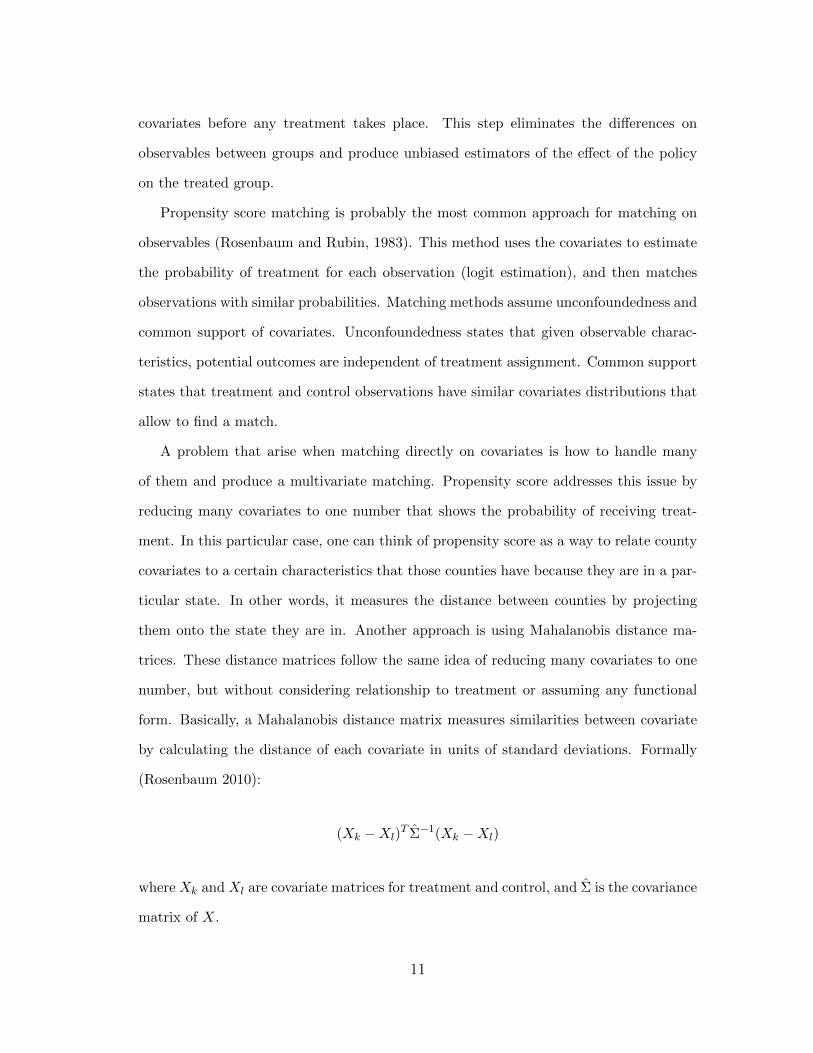
them onto the state they are in. Another approach is using Mahalanobis distance ma-

trices. These distance matrices follow the same idea of reducing many covariates to one

number, but without considering relationship to treatment or assuming any functional

form. Basically, a Mahalanobis distance matrix measures similarities between covariate

by calculating the distance of each covariate in units of standard deviations. Formally

(Rosenbaum 2010):

(Xk −Xl)T Σ̂−1(Xk −Xl)

where Xk and Xl are covariate matrices for treatment and control, and Σ̂ is the covariance

matrix of X.

11

As Rosenbaum (2010) pointed out, Mahalanobis distance matrix works best when data

is normally distributed. Because it used standard deviation as a measure of distance, this

is not the best approach when the data has outliers or a long-tailed distribution. In those

cases, the standard deviation will be inflated given less weight to covariates with those

distributions. This is an actual problem in my dataset, where counties may have huge

differences in covariates. As an example, a county in Illinois may greatly differ on the

amount of forest cover with respect to a county in Maryland. This will give that particular

covariate a smaller weight when calculating the distance matrix, and a mismatch on that

covariate will be less penalized compared to a mismatch on other covariates.

A rank-based Mahalanobis distance is a plausible solution to this problem. The key

aspect of this distance matrix is that it uses the ranking of the values of each covariate

and an adjusted covariance matrix 2 of these ranks to calculate the Mahalanobis distance

matrix. This method solves the problem of extreme outliers and long-tailed distributions.

I use Propensity Score and Rank-based Mahalanobis to calculate distance matrices that

are used for matching.

The second decision to make is the type of matching that better adapts to the prob-

lem under analysis. I use optimal full matching which allows the matching of one treated

unit to multiple controls, as well as one control to multiply treated units. Full matching

produces matching sets that are as close as those produced by pair matching or matching

with variable number of controls, and often closer matches come out. It is the optimal

matching method that minimizes the weighted average distance (Rosenbaum, 1991). Ap-

plications of this method can be found in Hansen (2004), Hansen and Klopfer (2006),

Stuart and Green (2008), and Heller et al (2009), to name a few.

Full matching minimizes the distance between all pairs within each matched sets and

across all data. The number of treated and control units in each matched set will depend

on covariates’ similarities, number of treated and control units, and the full matching

2The adjusted covariance matrix consists of pre and postmultiplying the rank covariance matrix by a diagonalmatrix where the diagonal elements are the ratio between the standard deviation of tied ranks and the standarddeviation of untied ranks (Rosenbaum, 2010).

12

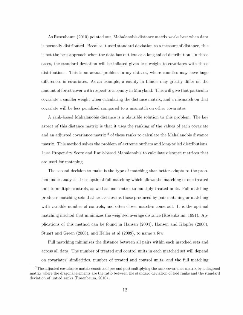
algorithm. 3 Following Rosenbaum (1991) and Hansen (2004), for each pair {c, t}, with

c ∈ C and t ∈ T , let dij ∈ [0,∞] be the corresponding distance for the ij observation in

the distance matrix, the full matching minimizes:

∑i∈T,S(i)>0

∑j∈C,S(i)=S(j)

dij

where S(i) is a mapping that defines the matched sets. An algorithm that explains how

optimal full matching works can be found in Hansen (2004) Appendix.

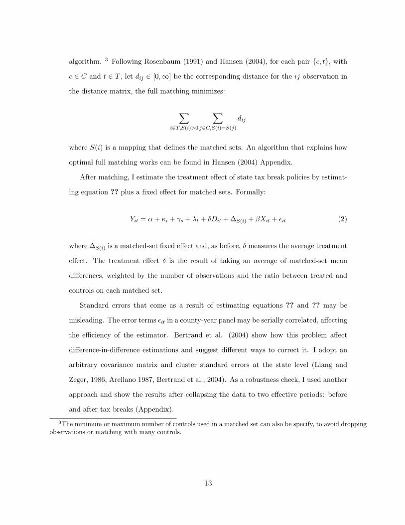
After matching, I estimate the treatment effect of state tax break policies by estimat-

ing equation ?? plus a fixed effect for matched sets. Formally:

Yit = α+ κi + γs + λt + δDit + ∆S(i) + βXit + εit (2)

where ∆S(i) is a matched-set fixed effect and, as before, δ measures the average treatment

effect. The treatment effect δ is the result of taking an average of matched-set mean

differences, weighted by the number of observations and the ratio between treated and

controls on each matched set.

Standard errors that come as a result of estimating equations ?? and ?? may be

misleading. The error terms εit in a county-year panel may be serially correlated, affecting

the efficiency of the estimator. Bertrand et al. (2004) show how this problem affect

difference-in-difference estimations and suggest different ways to correct it. I adopt an

arbitrary covariance matrix and cluster standard errors at the state level (Liang and

Zeger, 1986, Arellano 1987, Bertrand et al., 2004). As a robustness check, I used another

approach and show the results after collapsing the data to two effective periods: before

and after tax breaks (Appendix).

3The minimum or maximum number of controls used in a matched set can also be specify, to avoid droppingobservations or matching with many controls.

13

5 Results

I concentrate my analysis on the East Region of United States. I present results

from a fixed effect panel estimation using both raw data and a matched sample. All

approaches show a positive and significant effect of the implementation of a tax break

policy. Matching estimation also improves balance between treated and control groups.

Finally, I include some other specifications to account for anticipatory effects and also

decompose the effect of tax breaks in future years.

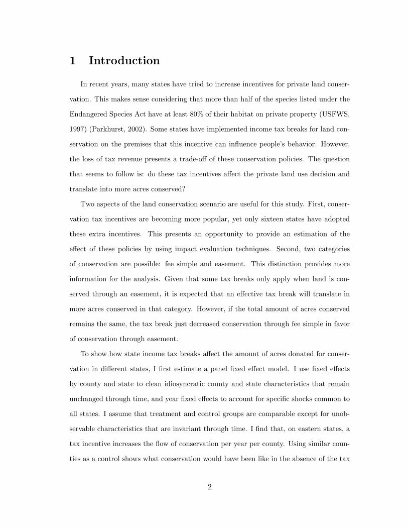
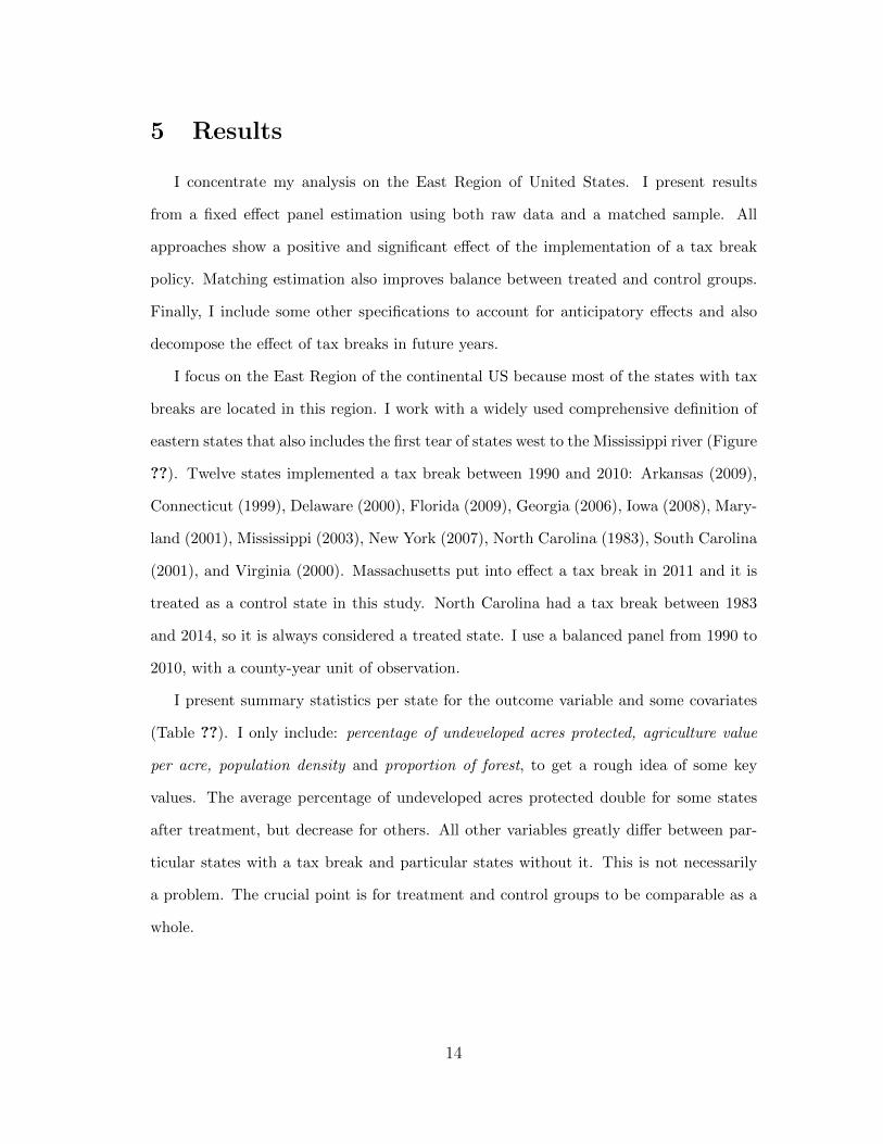
I focus on the East Region of the continental US because most of the states with tax

breaks are located in this region. I work with a widely used comprehensive definition of

eastern states that also includes the first tear of states west to the Mississippi river (Figure

??). Twelve states implemented a tax break between 1990 and 2010: Arkansas (2009),

Connecticut (1999), Delaware (2000), Florida (2009), Georgia (2006), Iowa (2008), Mary-

land (2001), Mississippi (2003), New York (2007), North Carolina (1983), South Carolina

(2001), and Virginia (2000). Massachusetts put into effect a tax break in 2011 and it is

treated as a control state in this study. North Carolina had a tax break between 1983

and 2014, so it is always considered a treated state. I use a balanced panel from 1990 to

2010, with a county-year unit of observation.

I present summary statistics per state for the outcome variable and some covariates

(Table ??). I only include: percentage of undeveloped acres protected, agriculture value

per acre, population density and proportion of forest, to get a rough idea of some key

values. The average percentage of undeveloped acres protected double for some states

after treatment, but decrease for others. All other variables greatly differ between par-

ticular states with a tax break and particular states without it. This is not necessarily

a problem. The crucial point is for treatment and control groups to be comparable as a

whole.

14

5.1 Matching and Panel Estimation

Difference-in-Difference based the estimation on the assumption that both groups,

treatment and control, are comparable except for unobservable characteristics that are

invariant through time. I first present results for a fixed effect panel estimation. Then,

I adjust comparability between groups using full matching and re-estimate the panel

model. I also include some specifications to consider lagged and anticipatory effects of

tax breaks.

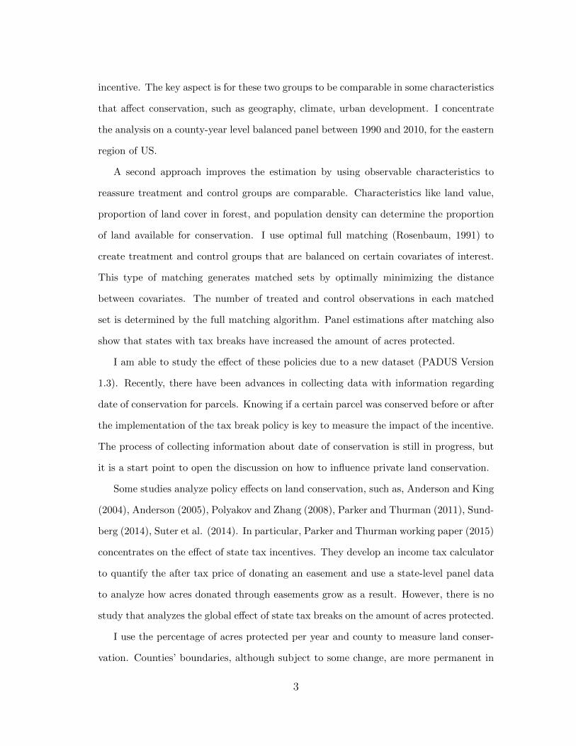
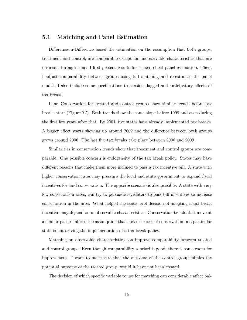
Land Conservation for treated and control groups show similar trends before tax

breaks start (Figure ??). Both trends show the same slope before 1999 and even during

the first few years after that. By 2001, five states have already implemented tax breaks.

A bigger effect starts showing up around 2002 and the difference between both groups

grows around 2006. The last five tax breaks take place between 2006 and 2009 .

Similarities in conservation trends show that treatment and control groups are com-

parable. One possible concern is endogeneity of the tax break policy. States may have

different reasons that make them more inclined to pass a tax incentive bill. A state with

higher conservation rates may pressure the local and state government to expand fiscal

incentives for land conservation. The opposite scenario is also possible. A state with very

low conservation rates, can try to persuade legislators to pass bill incentives to increase

conservation in the area. What helped the state level decision of adopting a tax break

incentive may depend on unobservable characteristics. Conservation trends that move at

a similar pace reinforce the assumption that lack or excess of conservation in a particular

state is not driving the implementation of a tax break policy.

Matching on observable characteristics can improve comparability between treated

and control groups. Even though comparability a priori is good, there is some room for

improvement. I want to make sure that the outcome of the control group mimics the

potential outcome of the treated group, would it have not been treated.

The decision of which specific variable to use for matching can considerable affect bal-

15

ance between groups. There is a trade-off between balance and final number of matched

sets that will depend on the variables used for matching and the distance matrix. De-

pending on the treated and control samples, matching on some covariates can significantly

reduce the number of matched sets. Variables that differ significantly between groups

are difficult to match. However, if those variables are important for conservation, they

cannot be left out.

I use a set of covariates to create two distance matrices using propensity score and

rank-based mahalanobis distance, respectively. I consider all variables at the same point

in time, the year 1998, before any tax break started. The set of covariates are: average

rate of undeveloped land protected per year between 1990 and 1998, cumulative per-

centage of undeveloped land protected, percentage of farms, agriculture value per acre,

unemployment rate, median household income, population density, percentage of votes

cast for democrats in presidential election, and proportion of land covered in forest4.

Forest areas are generally the focus for conservation, providing clean air and wild habitat

for different species.

The chosen covariates for matching influence conservation in different ways. One

would expect that counties with more acres in forest will also have more acres protected.

Similarly, landowners can place an easement on their farms and conserve that area,

restricting development but with the possibility of keeping the agriculture use of the area.

The opposite will probably be true for highly populated areas. Including the cumulative

percentage of undeveloped land protected is a good baseline and helps matching counties

that were alike in the amount of protection before treatment. However, it also assumes

that counties with similar percentage of land protected are also similar in their future

conservation trends. Matching on the average rate of undeveloped land protected can

minimize this potential problem. I use proportion (or percentage) of areas (farms, forest,

acres protected) to account for county size.

I use full matching using a propensity score distance matrix with a caliper of 0.1

4Proportion of forest correspond to the year 1992

16

standard deviation. From 421 treated and 775 control counties, this matching construct

165 matched pairs. It drops 1 treated and 9 control counties. The dropped treated county

is Pickens (South Carolina), home of Table Rock State Park. Forest cover approximately

77% of the county area. Dropped control counties are from Illinois (3), Kentucky (2),

Louisiana (1), Minnesota (1), New Hampshire (1), and Vermont (1). They show an

extremely low or extremely high rate of conservation between 1990 and 1998. They are

also outliers in terms of percentage of farms and proportion of forest.

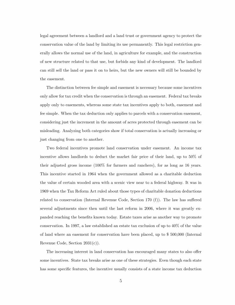
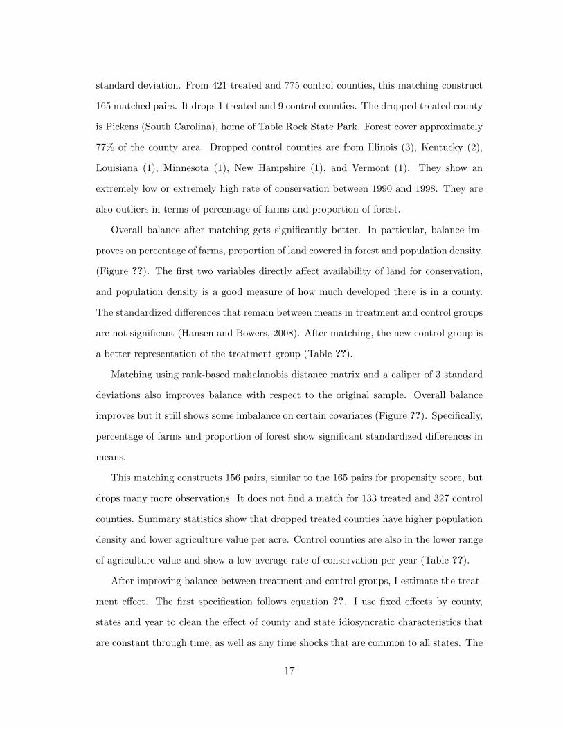
Overall balance after matching gets significantly better. In particular, balance im-

proves on percentage of farms, proportion of land covered in forest and population density.

(Figure ??). The first two variables directly affect availability of land for conservation,

and population density is a good measure of how much developed there is in a county.

The standardized differences that remain between means in treatment and control groups

are not significant (Hansen and Bowers, 2008). After matching, the new control group is

a better representation of the treatment group (Table ??).

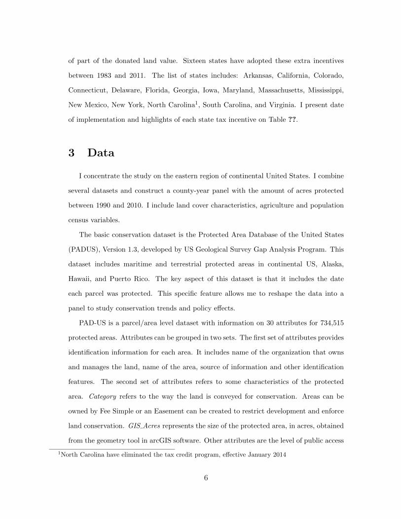
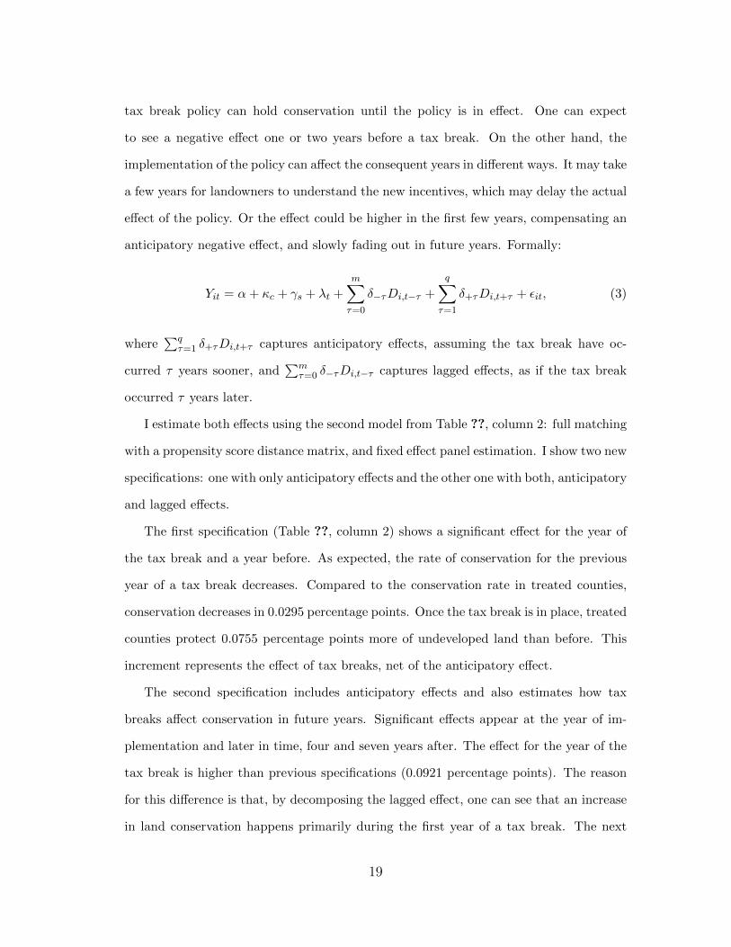
Matching using rank-based mahalanobis distance matrix and a caliper of 3 standard

deviations also improves balance with respect to the original sample. Overall balance

improves but it still shows some imbalance on certain covariates (Figure ??). Specifically,

percentage of farms and proportion of forest show significant standardized differences in

means.

This matching constructs 156 pairs, similar to the 165 pairs for propensity score, but

drops many more observations. It does not find a match for 133 treated and 327 control

counties. Summary statistics show that dropped treated counties have higher population

density and lower agriculture value per acre. Control counties are also in the lower range

of agriculture value and show a low average rate of conservation per year (Table ??).

After improving balance between treatment and control groups, I estimate the treat-

ment effect. The first specification follows equation ??. I use fixed effects by county,

states and year to clean the effect of county and state idiosyncratic characteristics that

are constant through time, as well as any time shocks that are common to all states. The

17

second and third specifications follow equation ??. These also include fixed effects for

each matched set and an treatment term that averages the effect for the whole sample.

The matrix of covariates includes: percentage of farms, average farm size, agriculture

value per acres, unemployment, median household income, population density and per-

centage of votes cast for democrats in presidential elections. The dependent variable is

the percentage of undeveloped land protected per year (Table ??).

Results are similar for all three specifications. Panel estimation without matching

show that tax breaks have a positive and significant results on the amount of acres

protected. Tax breaks increase the percentage of undeveloped land protected in 0.0708

percentage points (Column 1) in counties with tax break. Both matching estimations

slightly increase the coefficient of interest. Rank-based mahalanobis shows the highest

effect of a tax break, but reduces the amount of observations in almost one third. Also,

the balance between treatment and control was not that good. Propensity score improves

balance of the sample without dropping too many observations. It estimates an effect of a

tax break of 0.0712 percentage points for treated counties (Column 2). A treated county

protects on average at a rate of 0.06% undeveloped land per year. All panel estimations

suggest that after a tax break a treated county will more than doubled the rate at which

it protects undeveloped land, reaching between 0.13% and 0.14% per year.

Anticipatory Effects

Effects of a tax break policy may affect conservation rates differently at different

points in time. Landowners may react to a tax break a couple of years before it starts,

and may have a dynamic response a few years after its implementation. I present the

results with this new specification and explain the effects in terms of the amount of acres

protected.

I consider both anticipatory and lagged effects to pinpoint differences in conservation

rates per year before and after tax breaks. On the one hand, the announcement of a

18

tax break policy can hold conservation until the policy is in effect. One can expect

to see a negative effect one or two years before a tax break. On the other hand, the

implementation of the policy can affect the consequent years in different ways. It may take

a few years for landowners to understand the new incentives, which may delay the actual

effect of the policy. Or the effect could be higher in the first few years, compensating an

anticipatory negative effect, and slowly fading out in future years. Formally:

Yit = α+ κc + γs + λt +m∑τ=0

δ−τDi,t−τ +

q∑τ=1

δ+τDi,t+τ + εit, (3)

where∑q

τ=1 δ+τDi,t+τ captures anticipatory effects, assuming the tax break have oc-

curred τ years sooner, and∑m

τ=0 δ−τDi,t−τ captures lagged effects, as if the tax break

occurred τ years later.

I estimate both effects using the second model from Table ??, column 2: full matching

with a propensity score distance matrix, and fixed effect panel estimation. I show two new

specifications: one with only anticipatory effects and the other one with both, anticipatory

and lagged effects.

The first specification (Table ??, column 2) shows a significant effect for the year of

the tax break and a year before. As expected, the rate of conservation for the previous

year of a tax break decreases. Compared to the conservation rate in treated counties,

conservation decreases in 0.0295 percentage points. Once the tax break is in place, treated

counties protect 0.0755 percentage points more of undeveloped land than before. This

increment represents the effect of tax breaks, net of the anticipatory effect.

The second specification includes anticipatory effects and also estimates how tax

breaks affect conservation in future years. Significant effects appear at the year of im-

plementation and later in time, four and seven years after. The effect for the year of the

tax break is higher than previous specifications (0.0921 percentage points). The reason

for this difference is that, by decomposing the lagged effect, one can see that an increase

in land conservation happens primarily during the first year of a tax break. The next

19

significant increases happen at years four and seven, 0.0243 and 0.0759 percentage points,

respectively. This reinforces the hypothesis that, after the first response to a tax break.

it may take a while for landowners to learn about the new incentive and decide to protect

their land.

The question that follows is how much more land is protected as a result of a tax

break incentive. Percentage points show that the average conservation rate more than

doubles after the tax break. But what does this mean in terms of acres protected? I

show conservation rates and the amount of acres protected on an average treated county

(Table ??).

Estimations show how tax breaks affect conservation on treated counties. An average

treated county’s undeveloped area represents almost 94% of its total area. This translates

in approximately 420,000 acres. Counties with a tax break protect, on average, 0.0654%

of their undeveloped land the year before a tax break (approximately 27, 500 acres). The

rate of conservation for the year before a tax break is calculated as an average for the

calendar year before a treated county puts in place a tax break incentive. The first

estimation in table ?? show an increase of 0.0709 percentage points that translate in a

new conservation rate of 0.1363% per year (Table ??, row 1). In terms of the amount of

acres protected, this means that tax breaks will result in 57, 000 acres protected every

year on an average treated counties. This estimation does not consider any anticipatory

or lagged effects

Including anticipatory effects show how information on upcoming law changes can

affect land conservation decisions. Two years before tax breaks incentives start, treated

counties protect land at a rate of 0.0937%. This average is the rate of conservation at

t − 2. At this time, treated counties protected on average 39, 000 acres per year. The

second specification in Table ?? shows that the year before a tax break, i.e. t − 1, the

rate of land conservation decreases in −0.295 percentage points. One can observed on

average 27, 000 acres protected that year, 12, 000 acres less compared to a year before.

The yearly rate of conservation reaches 0.14% for the first year of a tax break, and the

20

amount of acres protected is on average 59, 000 (at t). This shows the net effect for the

first year of a tax break, probably higher compensating for some reduction due to the

anticipatory effect. After the decrease of conservation the year before, once the tax break

is in place, landowners who were waiting move forward and donate their land.

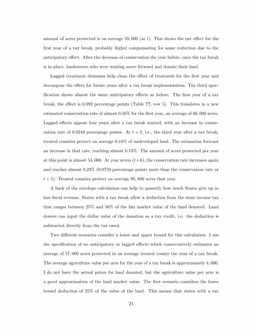
Lagged treatment dummies help clean the effect of treatment for the first year and

decompose the effect for future years after a tax break implementation. The third spec-

ification shows almost the same anticipatory effects as before. The first year of a tax

break, the effect is 0.092 percentage points (Table ??, row 5). This translates in a new

estimated conservation rate of almost 0.16% for the first year, an average of 66, 000 acres.

Lagged effects appear four years after a tax break started, with an increase in conser-

vation rate of 0.0243 percentage points. At t + 2, i.e., the third year after a tax break,

treated counties protect on average 0.10% of undeveloped land. The estimation forecast

an increase in that rate, reaching almost 0.13%. The amount of acres protected per year

at this point is almost 54, 000. At year seven (t+6), the conservation rate increases again

and reaches almost 0.23% (0.0759 percentage points more than the conservation rate at

t+ 5). Treated counties protect on average 95, 800 acres that year.

A back of the envelope calculation can help to quantify how much States give up in

loss fiscal revenue. States with a tax break allow a deduction from the state income tax

that ranges between 25% and 50% of the fair market value of the land donated. Land

donors can input the dollar value of the donation as a tax credit, i.e. the deduction is

subtracted directly from the tax owed.

Two different scenarios consider a lower and upper bound for this calculation. I use

the specification of no anticipatory or lagged effects which conservatively estimates an

average of 57, 000 acres protected in an average treated county the year of a tax break.

The average agriculture value per acre for the year of a tax break is approximately 4, 000.

I do not have the actual prices for land donated, but the agriculture value per acre is

a good approximation of the land market value. The first scenario considers the lower

bound deduction of 25% of the value of the land. This means that states with a tax

21

break get $1, 000 less per acres protected (4, 000× 0.25). The second scenario considers

an upper bound, with a deduction of 50% of the land value. These states get on average

$2, 000 less per acres protected (4, 000× 0.50).

Since in an average treated county landowners donate 57, 000 acres the year of a tax

break, the average deduction can range between $57 and $114 millions for the State

(57, 000× 4, 000× 0.25 and 57, 000× 4, 000× 0.5). Because some states have a tax credit

limits per year, this deduction is sometimes carried over several years. However, the total

amount deducted in the end will still be the total amount presented here.

5.2 Risk Set Matching

A second approach to matching uses the full panel instead of only data before any

treatment for matching.This is known as risk-set matching and it refers to matching ob-

servations that are ”at risk of receiving treatment”, before they are treated (Rosenbaum,

2010). The theory of this type of matching is explained in Li et al. (2001), and some

applications include Wu et al. (2008), Rosenbaum and Silber (2009), Silber et al. (2009),

Nieuwbeerta et al. (2009).

I match treated county-year observations with control county-year observations. Con-

trol counties are all observations that were never treated and if they were, I use only all

years before treatment. Treated counties are the ones with a tax break, but only the

first year of treatment 5. This reduces the matching set to 22, 161 observations, 421

treated and 21, 740 controls. Before dropping treated observations after the first year of

treatment, I calculate the average percentage of undeveloped land protected per year five

years in the future. I use this later as the dependent variable to measure the effect of the

tax break incentive.

I use the same two methods to build two different distance matrices: propensity

score and rank-based mahalanobis. The set of covariates to calculate distances for both

5After a tax break is in place, the treated county is always treated. Once that county-year observation ismatched with a control, it cannot be used anymore

22

methods includes: cumulative percentage of undeveloped land protected the year before a

tax break, agriculture value per acre, population density and proportion of forest. Three

other distance matrices work as penalties to avoid certain types of matching. The first

penalty matrix avoids matching counties with itself. The second penalty matrix avoids

matching a treated county with a control one from a later year. The third penalty matrix

does not allow matching a treated county with a control county that will become treated

in the next five years. The final two distance matrices include the base propensity score

or rank-based mahalanobis distance matrix, with the three penalty matrices.

Optimal full matching based on the propensity score results in better balanced treat-

ment and control groups. Some of the covariates show less standardized mean differences

compared to the raw sample. There are still some significant standardize differences in

agriculture value per acres and proportion of forest, although their values are not that

high (Figure ??). Overall balance for the whole sample improves.

Using a rank-based mahalanobis distance matrix improves balance relative to propen-

sity score distance matrix. The standardize difference in mean for agriculture value per

acres is still significant, but the other three covariates do not show significant standardize

differences (Figure ??). Overall balance is better compared to the raw sample and similar

to the one achieved with propensity score.

After full matching both approaches yield similar results. Propensity score drops 33

treated county-year observations and 1663 control county-year observations. It matches

only 4 one-to-one pairs. Rank-based mahalanobis drops 32 treated county-year obser-

vations and 1,682 control county-year observations. It forms 25 one-to-one pairs. The

final number of observations is similar for both, 20,465 and 20,447 respectively. Finally,

I estimate a modified version of equation ??, where the dependent variable is the average

percentage of undeveloped acres protected per year, during the five years that follow a

tax break incentive.

Results of risk set matching with panel estimation are similar for both, propensity

score and rank-based mahalanobis (Table ??) . Using rank-based mahalanobis distance

23

matrix shows a higher effect of tax breaks compared to propensity score. Including a

a matrix of covariates improves the adjustment of the model and slightly reduces the

coefficient of interest. Results are comparable to the other matching approach. Using

rank-based mahalanobis distance matrix seem to be the better approach for risk set

matching since it improves balance and it does not drop many observations.

5.3 Robustness checks

I expand the analysis to make sure results are robust to misspecifications. First, I

estimate the effect of tax breaks with randomly generated placebo laws. Second, I test

robustness of standard errors correction using two different approaches: a Monte Carlo

simulation for placebo laws and collapsing data into pre and post treatment periods

(Bertrand et at., 2004).

Placebo Laws

Placebo laws can be useful to check how the model performs. Randomly generated

placebo tax breaks should not show any effect on land conservation. I generate placebo

laws for two samples and estimate equations ?? and ??. I find no effect of this placebo

laws on the yearly rate of conservation.

One way to check robustness of results is to randomly assign treatment to treated

and/or control states and see how the model performs. Under this assumption, there is

no reason to believe that this placebo treatment will show any effect on land conservation.

One would expect that previous estimations show the actual effect of tax break laws, and

that the increase in conservation is not just randomly explained by the data itself. I

choose two different sets of states and assign random treatment to check this hypothesis.

The first approach takes a sample of all the states on the east region that never had

a tax break. This sample consists of 18 states with no tax break between 1990 and 2010.

I then randomly select five of those states and assign a tax break law for a specific year.

24

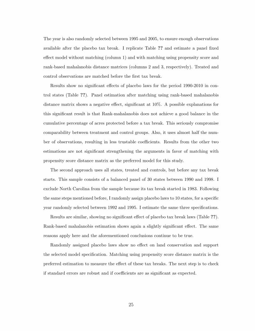
The year is also randomly selected between 1995 and 2005, to ensure enough observations

available after the placebo tax break. I replicate Table ?? and estimate a panel fixed

effect model without matching (column 1) and with matching using propensity score and

rank-based mahalanobis distance matrices (columns 2 and 3, respectively). Treated and

control observations are matched before the first tax break.

Results show no significant effects of placebo laws for the period 1990-2010 in con-

trol states (Table ??). Panel estimation after matching using rank-based mahalanobis

distance matrix shows a negative effect, significant at 10%. A possible explanations for

this significant result is that Rank-mahalanobis does not achieve a good balance in the

cumulative percentage of acres protected before a tax break. This seriously compromise

comparability between treatment and control groups. Also, it uses almost half the num-

ber of observations, resulting in less trustable coefficients. Results from the other two

estimations are not significant strengthening the arguments in favor of matching with

propensity score distance matrix as the preferred model for this study.

The second approach uses all states, treated and controls, but before any tax break

starts. This sample consists of a balanced panel of 30 states between 1990 and 1998. I

exclude North Carolina from the sample because its tax break started in 1983. Following

the same steps mentioned before, I randomly assign placebo laws to 10 states, for a specific

year randomly selected between 1992 and 1995. I estimate the same three specifications.

Results are similar, showing no significant effect of placebo tax break laws (Table ??).

Rank-based mahalanobis estimation shows again a slightly significant effect. The same

reasons apply here and the aforementioned conclusions continue to be true.

Randomly assigned placebo laws show no effect on land conservation and support

the selected model specification. Matching using propensity score distance matrix is the

preferred estimation to measure the effect of these tax breaks. The next step is to check

if standard errors are robust and if coefficients are as significant as expected.

25

Robustness of Standard Errors

First Approach: Monte Carlo and Placebo Laws

A Monte Carlo exercise with placebo laws can help to support the method selected

for correcting serially correlated errors. I follow Bertrand et al. (2004) and randomly

select states with no tax break and assign them treatment at random years. One expect

to reject the null hypothesis of no effect around 5% of the times, at a significant level of

5%.

I use the same two samples as before for this exercise. First I use a sample of all states

that never had a tax break (18 states, for the period 1990-2010). Then, I use a second

sample of all states before any tax break started (30 states, for the period 1990-1998).

I follow the same steps as before and randomly assign placebo laws for specific years.

For each sample, I run a Monte Carlo experiment of 200 simulations, where I estimate

equation ?? for 300 different placebo laws assignment.

Results are different depending on how standard errors are calculated. I report the

average rejection rate where the absolute value of the t-statistics is bigger than 1.96

(Table ??). The first t-value corresponds to not corrected standard errors, ignoring

serial correlation. It shows that 26% of the times the model finds an effect of tax break

laws, where in fact no such effect exists. After clustering standard errors by state, the

rejection rate drops to almost 7% (first row of Table ??). The second sample shows

similar results. When errors are not corrected, the rejection rate climbs to a 21%, while

clustering standard errors by state shows that 6.8% of the times placebo laws show no

effect.

This approach shows that in this particular problem, clustering standard errors by

state helps correct the serial correlation. Rejection rates of the null hypothesis of no effect

drop to their expected values when standard errors are clustered by state. This exercise

reinforces the assumption that errors are serially correlated. The variance-covariance

26

matrix appears to be block diagonal by state.

Second Approach: Collapsing Data, Pre and Post Treatment

Collapsing data to two effective periods is straightforward when treatment happens

at one point in time for all treated observations. However, when treatment takes place at

different times, this method may be not possible for all the sample. In this particular case

I reduce the sample and use as treated only states that passed a tax break law between

1999 and 2001. Connecticut started the tax break incentive in 1999, Delaware and

Virginia in 2000 and finally Maryland and South Carolina in 2001. I dropped observations

on eastern states that implemented a tax break after 2001 but before 2010: Mississippi

(2003), Georgia (2006), New York (2007), Iowa (2008), Arkansas (2009) and Florida

(2009). North Carolina has had a tax break since 1983, so it was also dropped from the

analysis. All other states in the eastern region are considered control states.

I estimate two specifications. First I estimate a simple before and after difference-in-

difference model. I define acres protected before and after the tax break as follows: acres

protected before is the average of undeveloped land protected per year between 1991 and

1998, acres protected after corresponds to the average of undeveloped land protected per

year between 2002 and 2009. I use the same set of covariates as before, at a specific point

in time: 1998 and 2009. Second, I estimate the same model with a matched sample and

a fixed effect for matched groups. I match on observable characteristics before any tax

break is in effect (1998).

Results show a positive and significant effect of tax breaks. The coefficient of interest

is different than the one estimated with a panel model. This is reasonable because both

samples are actually different. In the difference-in-difference approach some states are

left out. Furthermore, the dependent variable is a difference in average before and after

treatment. This removes the effect of an increasing conservation trend and increases

the difference before and after treatment. However, results are comparable to panel

27

estimations with standard errors clustered by state. The specific equations and tables

can be found in the Appendix.

6 Concluding Remarks

This study is a general approach to measure the effect of State Tax Breaks on the

average percentage of acres protected per year. It concentrates on a extended region, a

comprehensive definition of eastern states of United States, which provides a big picture

of the incentive’s effect. One should interpret the results presented here as a first approach

to quantify the overall effect of these policies. Other studies have analyzed the effect of

a state tax incentive at a smaller scale, but this exceeds the scope of this paper.

State tax breaks for conservation have a positive and significant effect when analyzing

their effect on the eastern states. All estimations show that implementing a tax break

increases the rate at which counties protect undeveloped area. An average treated county

protects undeveloped land at a rate of almost 0.14% after a tax break starts. This suggests

that the rate of conservation more than doubles for counties with a tax break. In terms of

acreage, this new rate represents an average area of approximately 57, 000 acres protected

every year.

Effects of a tax break are not uniform in all years. Considering anticipatory and

lagged effects show how these incentives have a different effect at different points in time.

A year before a tax break, the rate of conservation decreases in 0.0292 percentage points,

an average of 12, 000 acres less protected. The first year of a tax break, the rate has a

peak increasing 0.0921 percentage points and treated counties protect on average 66, 000

acres that year. Tax breaks have no significant effect for the next two years, showing

again a positive and significant effect four and seven years after they started.

Optimal full matching improves balance between covariates. Looking at raw data,

treated and control counties conservation trends are similar. Nevertheless, matching on

observables refine balance between both groups, making them more comparable. Propen-

28

sity Score distance matrix shows better balance and does not drop many observations,

making it the preferred approach. Its results are robust when tested under randomly

generated placebo laws.

Although tax incentives lead to increase in conservation, an important trade-off also

emerges. Further analysis needs to explore how big these tax credits are in terms of less

tax revenue for the states implementing the deduction. A back of the envelope calculation

shows the loss in revenue for states with a tax break is between $1000 and $2000 per

acre protected. This becomes an important issue when many of these states are facing

unbalanced budgets and increasing fiscal deficits. The efficient use of public resources is

generating more debate now. It is important to study if these policies actually accomplish

the goal for which they were design, and to measure the real effect they have. This will

help policy makers quantify the effect of the use of state resources, and help decide how

to target government spending according to their needs.

References

Anderson, C. M. and King, J. R. (2004). Equilibrium Behavior in the Conservation

Easement Game. Land Economics, 80(3):355–374.

Anderson, J. E. (2005). Taxes and fees as forms of land use regulation. The Journal of

Real Estate Finance and Economics, 31(4):413–427.

Angrist, J. D. and Pischke, J.-S. (2009). Mostly Harmless Econometrics: An Empiricist’s

Companion. Princeton University Press.

Arellano, M. (1987). Computing robust standard errors for within group estimators.

Ashenfelter, O. C. (1978). Estimating the effect of training programs on earnings. The

Review of Economics and Statistics, 60(1):47–57.

29

Ashenfelter, O. C. and Card, D. (1985). Using the longitudinal structure of earnings

to estimate the effect of training programs. The review of economics and statistics,

67(4):648–660.

Bertrand, M., Duflo, E., and Mullainathan, S. (2004). How Much Should We

Trust Difference-in-Difference Estimates? The Quarterly Journal of . . . , 119

(1)(February):249–275.

Chang, K. (2011). 2010 National Land Trust Census Report. A Look at Voluntary Land

Conservation in America. Technical report.

Hansen, B. B. (2004). Full Matching in an Observational Study of Coaching for the SAT.

Journal of the American Statistical Association, 99(467):609–618.

Hansen, B. B. and Bowers, J. (2008). Covariate Balance in Simple, Stratified and Clus-

tered Comparative Studies. Statistical Science, 23(2):219–236.

Hansen, B. B. and Klopfer, S. O. (2006). Optimal Full Matching and Related Designs

via Network Flows. Journal of Computational and Graphical Statistics, 15(3):609–627.

Heller, R., Manduchi, E., and Small, D. S. (2009). Matching methods for observational

microarray studies. Bioinformatics, 25(7):904–909.

Imbens, G. W. and Wooldridge, J. (2009). Recent developments in the econometrics of

program evaluation. Journal of Economic Literature, 47(1):5–86.

IRC (Internal Revenue Code). Tax Code, Regulations and Official Guidance.

Land Trust Alliance. Land Trust Alliance.

Li, Y. P., Propert, K. J., and Rosenbaum, P. R. (2001). Balanced Risk Set Matching.

Journal of the American Statistical Association, 96(455):870–882.

30

Liang, K.-Y. Y. and Zeger, S. L. (1986). Longitudinal data analysis using generalized

linear models. Biometrika, 73(1):13–22.

Nieuwbeerta, P., Nagin, D. S., and Blokland, A. a. J. (2009). Assessing the Impact of

First-Time Imprisonment on Offenders Subsequent Criminal Career Development: A

Matched Samples Comparison. Journal of Quantitative Criminology, 25:227–257.

Parker, D. and Thurman, W. (2011). Crowding Out Open Space: The Effects of Federal

Land Programs on Private Land Trust Conservation. Land Economics, 87(2):202–222.

Parker, D. P. and Thurman, W. N. (2015). Tax Incentives and the Price of Conservation.

Parkhurst, G., Shogren, J., and Bastian, C. (2002). Agglomeration bonus: an incentive

mechanism to reunite fragmented habitat for biodiversity conservation. Ecological

Economics, 41(2):305–328.

Polyakov, M. and Zhang, D. (2008). Property Tax Policy and Land-Use Change. Land

Economics, 84(3):396–408.

Rosenbaum, P. R. (1991). A characterization of optimal designs for observational studies.

Journal of the Royal Statistical Society: Series B (Methodological), 53(3):597–610.

Rosenbaum, P. R. (2010). Design of Observational Studies. Springer Series in Statistics.

Rosenbaum, P. R. and Rubin, D. B. (1983). The Central Role of the Propensity Score

in Observational Studies for Causal Effects. Biometrica, 70(1):41–55.

Rosenbaum, P. R. and Silber, J. H. (2009). Sensitivity Analysis for Equivalence and

Difference in an Observational Study of Neonatal Intensive Care Units. Journal of the

American Statistical Association, 104(486):501–511.

Silber, J. H., Lorch, S. a., Rosenbaum, P. R., Medoff-Cooper, B., Bakewell-Sachs, S.,

Millman, A., Mi, L., Even-Shoshan, O., and Escobar, G. J. (2009). Time to Send the

31

Preemie Home? Additional Maturity at Discharge and Subsequent Health Care Costs

and Outcomes. Health Services Research, 44(2):444–463.

Stuart, E. A. and Green, K. M. (2008). Using full matching to estimate causal effects

in nonexperimental studies: examining the relationship between adolescent marijuana

use and adult outcomes. Developmental Psychology, 44(2):395–406.

Sundberg, J. (2014). Preferential Assessment for Open Space. Public Finance and Man-

agement, 14(2):165–193.

Suter, J. F., Dissanayake, S., and Lewis, L. (2014). Public Incentives for Conservation

Easements on Private Land.

US Geological Service. National Gap Analysis Program: USGS Core Sciences Analytics

and Synthesis.

US Geological Survey - GAP Analysis Program (GAP). Protected Areas Database of the

United States (PADUS).

Wu, J. and Irwin, E. G. (2008). Optimal Land Development with Endogenous Environ-

mental Amenities. American Journal of Agricultural Economics, 90(1):232–248.

32

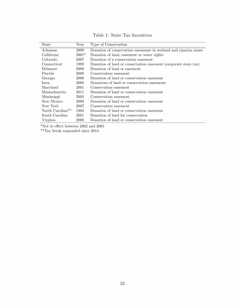
Table 1: State Tax Incentives

State Year Type of Conservation

Arkansas 2009 Donation of conservation easements in wetland and riparian zonesCalifornia 2001* Donation of land, easement or water rightsColorado 2007 Donation of a conservation easementConnecticut 1999 Donation of land or conservation easement (corporate state tax)Delaware 2000 Donation of land or easementFlorida 2009 Conservation easementGeorgia 2006 Donation of land or conservation easementIowa 2008 Donations of land or conservation easementsMaryland 2001 Conservation easementMassachusetts 2011 Donation of land or conservation easementMississippi 2003 Conservation easementNew Mexico 2008 Donation of land or conservation easementNew York 2007 Conservation easementNorth Carolina** 1983 Donation of land or conservation easementSouth Carolina 2001 Donation of land for conservationVirginia 2000 Donation of land or conservation easement

*Not in effect between 2002 and 2005**Tax break suspended since 2014

33

Table 2: Summary Statistics

% Undeveloped Protected Ag. Value per Acre Population Density Proportion Forest

Control Treated Control Treated Control Treated Control TreatedState Mean Sd Mean Sd Mean Sd Mean Sd Mean Sd Mean Sd Mean Sd Mean SdAL 0.06 0.36 2092.95 621.71 124.26 103.06 0.64 0.17AR 0.03 0.29 1564.67 607.91 41.05 36.92 0.40 0.30CT 0.04 0.17 10121.48 4654.86 688.82 496.83 0.54 0.13DE 0.02 0.07 5483.37 3206.75 517.28 462.13 0.20 0.05FL 0.07 0.42 3913.99 3785.18 208.55 242.06 0.24 0.16GA 0.03 0.29 2963.55 2051.39 251.76 515.42 0.57 0.21IA 0.01 0.08 2182.37 792.58 52.80 55.09 0.10 0.09IL 0.04 0.33 2657.44 1123.20 196.72 641.95 0.15 0.12IN 0.03 0.36 2709.58 864.86 186.03 301.98 0.22 0.19KY 0.03 0.21 2129.16 1066.05 128.12 250.51 0.50 0.23LA 0.12 1.04 2202.70 3365.17 152.40 392.21 0.28 0.28MA 0.01 0.06 11590.26 7481.76 702.42 562.76 0.45 0.23MD 0.14 0.23 4567.58 2493.15 774.62 1636.18 0.33 0.17ME 0.26 1.35 2045.21 987.41 86.75 88.48 0.67 0.16MI 0.02 0.14 2361.37 1252.89 185.75 425.25 0.29 0.19MN 0.03 0.15 1752.18 985.87 77.04 231.43 0.14 0.14MO 0.02 0.12 1597.32 728.31 200.37 756.11 0.33 0.24MS 0.08 0.46 1314.19 547.08 52.02 37.49 0.29 0.24NC 0.01 0.08 3816.23 2164.77 249.77 316.21 0.54 0.28NH 0.34 0.97 3514.79 1780.48 170.24 143.33 0.77 0.09NJ 0.02 0.16 17694.39 23237.47 1879.78 2896.19 0.37 0.16NY 0.07 0.41 6682.84 20031.88 508.85 1208.97 0.55 0.22OH 0.04 0.52 3723.10 3260.63 518.68 722.84 0.33 0.20PA 0.04 0.14 4192.39 4162.17 573.35 1649.82 0.61 0.21RI 0.04 0.16 11648.49 6238.36 1135.98 575.19 0.37 0.21SC 0.07 0.41 2384.89 1179.10 160.54 131.12 0.49 0.14TN 0.02 0.14 2601.74 1084.68 148.75 236.35 0.59 0.26VA 0.15 0.50 2617.03 3735.87 640.92 1353.71 0.56 0.21VT 0.14 0.71 2216.21 757.00 68.96 58.85 0.70 0.19WI 0.02 0.18 2222.14 1187.35 205.38 552.46 0.31 0.21WV 0.04 0.43 1597.23 937.82 116.26 128.92 0.76 0.12

All Region 0.0456 0.419 0.0817 0.388 3008.54 5011.46 3446.79 7785.98 254.34 812.83 382.64 975.23 0.36 0.27 0.45 0.26

Figure 1: Treated and Control States - Eastern Region

34

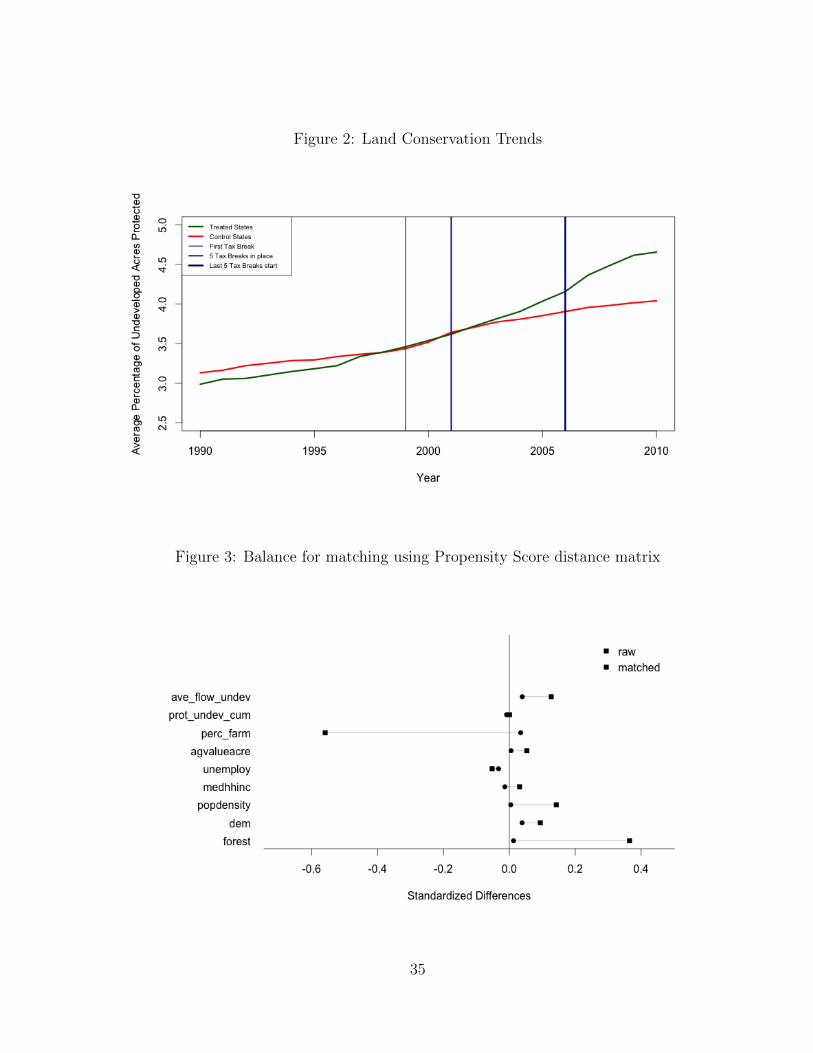
Figure 2: Land Conservation Trends

Figure 3: Balance for matching using Propensity Score distance matrix

35

Figure 4: Balance for matching using Rank-based Mahalanobis distance matrix

Figure 5: Balance after Risk Set Matching using Propensity Score distance matrix

36

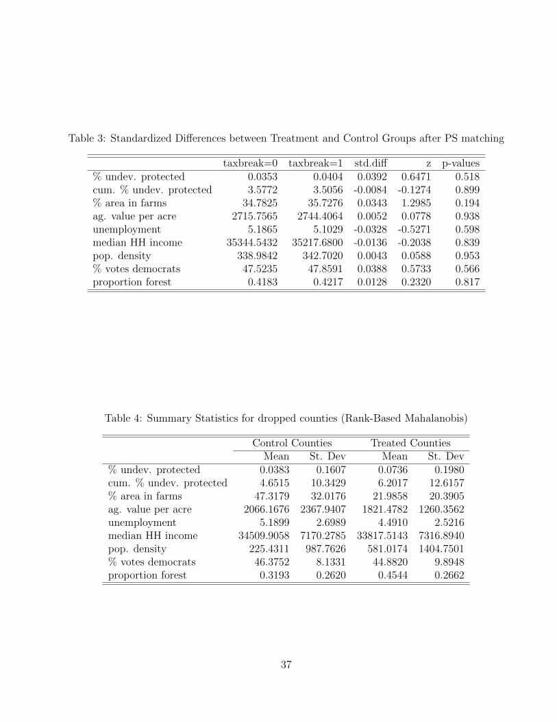
Table 3: Standardized Differences between Treatment and Control Groups after PS matching

taxbreak=0 taxbreak=1 std.diff z p-values% undev. protected 0.0353 0.0404 0.0392 0.6471 0.518cum. % undev. protected 3.5772 3.5056 -0.0084 -0.1274 0.899% area in farms 34.7825 35.7276 0.0343 1.2985 0.194ag. value per acre 2715.7565 2744.4064 0.0052 0.0778 0.938unemployment 5.1865 5.1029 -0.0328 -0.5271 0.598median HH income 35344.5432 35217.6800 -0.0136 -0.2038 0.839pop. density 338.9842 342.7020 0.0043 0.0588 0.953% votes democrats 47.5235 47.8591 0.0388 0.5733 0.566proportion forest 0.4183 0.4217 0.0128 0.2320 0.817

Table 4: Summary Statistics for dropped counties (Rank-Based Mahalanobis)

Control Counties Treated CountiesMean St. Dev Mean St. Dev

% undev. protected 0.0383 0.1607 0.0736 0.1980cum. % undev. protected 4.6515 10.3429 6.2017 12.6157% area in farms 47.3179 32.0176 21.9858 20.3905ag. value per acre 2066.1676 2367.9407 1821.4782 1260.3562unemployment 5.1899 2.6989 4.4910 2.5216median HH income 34509.9058 7170.2785 33817.5143 7316.8940pop. density 225.4311 987.7626 581.0174 1404.7501% votes democrats 46.3752 8.1331 44.8820 9.8948proportion forest 0.3193 0.2620 0.4544 0.2662

37

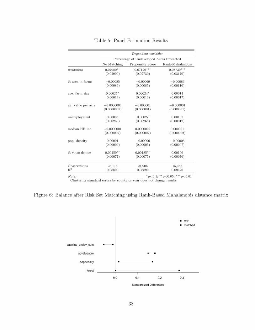
Table 5: Panel Estimation Results

Dependent variable:

Percentage of Undeveloped Acres Protected

No Matching Propensity Score Rank-Mahalanobis

treatment 0.07080∗∗ 0.07120∗∗∗ 0.08730∗∗∗

(0.02900) (0.02730) (0.03170)

% area in farms −0.00085 −0.00069 −0.00083(0.00086) (0.00085) (0.00110)

ave. farm size 0.00025∗ 0.00024∗ 0.00014(0.00014) (0.00013) (0.00017)

ag. value per acre −0.0000004 −0.000001 −0.000001(0.0000005) (0.000001) (0.000001)

unemployment 0.00035 0.00027 0.00107(0.00265) (0.00268) (0.00312)

median HH inc −0.0000001 0.0000002 0.000001(0.000002) (0.000002) (0.000002)

pop. density 0.00001 −0.00006 −0.00003(0.00009) (0.00005) (0.00007)

% votes democ 0.00159∗∗ 0.00185∗∗ 0.00106(0.00077) (0.00075) (0.00076)

Observations 25,116 24,906 15,456R2 0.08800 0.08890 0.09420

Note: ∗p<0.1; ∗∗p<0.05; ∗∗∗p<0.01Clustering standard errors by county or year does not change results

Figure 6: Balance after Risk Set Matching using Rank-Based Mahalanobis distance matrix

38

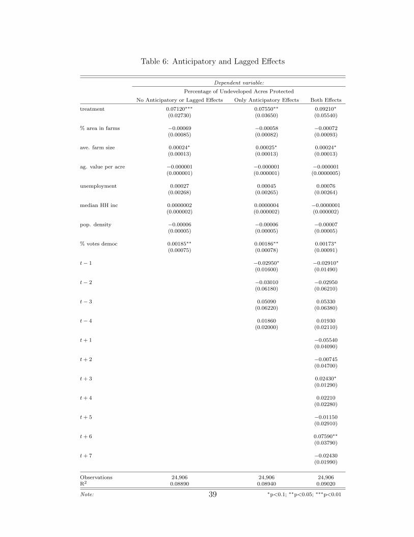
Table 6: Anticipatory and Lagged Effects

Dependent variable:

Percentage of Undeveloped Acres Protected

No Anticipatory or Lagged Effects Only Anticipatory Effects Both Effects

treatment 0.07120∗∗∗ 0.07550∗∗ 0.09210∗

(0.02730) (0.03650) (0.05540)

% area in farms −0.00069 −0.00058 −0.00072(0.00085) (0.00082) (0.00093)

ave. farm size 0.00024∗ 0.00025∗ 0.00024∗

(0.00013) (0.00013) (0.00013)

ag. value per acre −0.000001 −0.000001 −0.000001(0.000001) (0.000001) (0.0000005)

unemployment 0.00027 0.00045 0.00076(0.00268) (0.00265) (0.00264)

median HH inc 0.0000002 0.0000004 −0.0000001(0.000002) (0.000002) (0.000002)

pop. density −0.00006 −0.00006 −0.00007(0.00005) (0.00005) (0.00005)

% votes democ 0.00185∗∗ 0.00186∗∗ 0.00173∗

(0.00075) (0.00078) (0.00091)

t− 1 −0.02950∗ −0.02910∗

(0.01600) (0.01490)

t− 2 −0.03010 −0.02950(0.06180) (0.06210)

t− 3 0.05090 0.05330(0.06220) (0.06380)

t− 4 0.01860 0.01930(0.02000) (0.02110)

t+ 1 −0.05540(0.04090)

t+ 2 −0.00745(0.04700)

t+ 3 0.02430∗

(0.01290)

t+ 4 0.02210(0.02280)

t+ 5 −0.01150(0.02910)

t+ 6 0.07590∗∗

(0.03790)

t+ 7 −0.02430(0.01990)

Observations 24,906 24,906 24,906R2 0.08890 0.08940 0.09020

Note: ∗p<0.1; ∗∗p<0.05; ∗∗∗p<0.0139

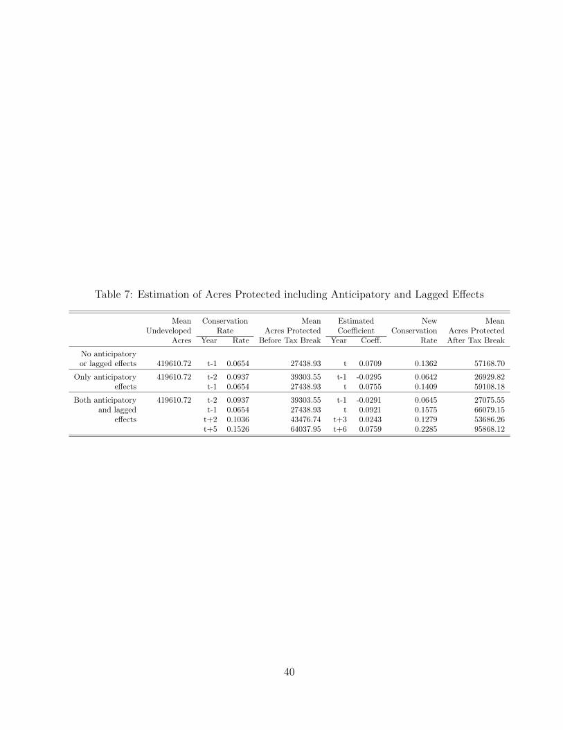
Table 7: Estimation of Acres Protected including Anticipatory and Lagged Effects

Mean Conservation Mean Estimated New MeanUndeveloped Rate Acres Protected Coefficient Conservation Acres Protected

Acres Year Rate Before Tax Break Year Coeff. Rate After Tax Break

No anticipatoryor lagged effects 419610.72 t-1 0.0654 27438.93 t 0.0709 0.1362 57168.70

Only anticipatory 419610.72 t-2 0.0937 39303.55 t-1 -0.0295 0.0642 26929.82effects t-1 0.0654 27438.93 t 0.0755 0.1409 59108.18

Both anticipatory 419610.72 t-2 0.0937 39303.55 t-1 -0.0291 0.0645 27075.55and lagged t-1 0.0654 27438.93 t 0.0921 0.1575 66079.15

effects t+2 0.1036 43476.74 t+3 0.0243 0.1279 53686.26t+5 0.1526 64037.95 t+6 0.0759 0.2285 95868.12

40

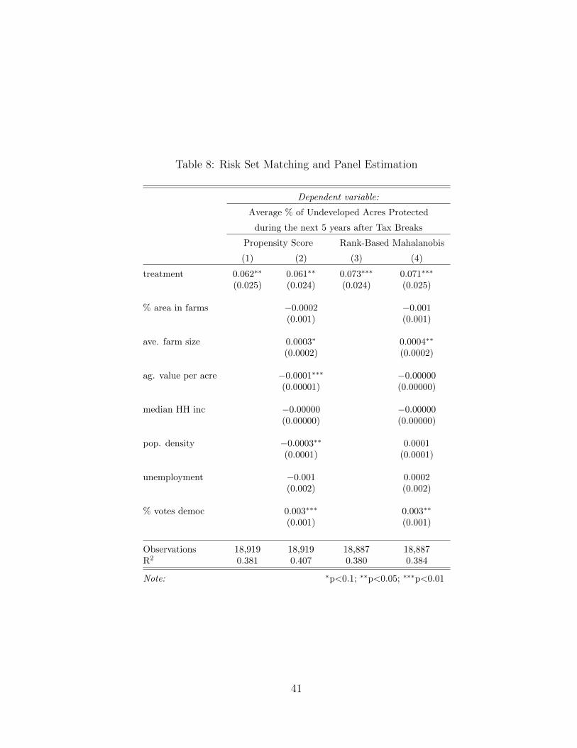
Table 8: Risk Set Matching and Panel Estimation

Dependent variable:

Average % of Undeveloped Acres Protected

during the next 5 years after Tax Breaks

Propensity Score Rank-Based Mahalanobis

(1) (2) (3) (4)

treatment 0.062∗∗ 0.061∗∗ 0.073∗∗∗ 0.071∗∗∗

(0.025) (0.024) (0.024) (0.025)

% area in farms −0.0002 −0.001(0.001) (0.001)

ave. farm size 0.0003∗ 0.0004∗∗

(0.0002) (0.0002)

ag. value per acre −0.0001∗∗∗ −0.00000(0.00001) (0.00000)

median HH inc −0.00000 −0.00000(0.00000) (0.00000)

pop. density −0.0003∗∗ 0.0001(0.0001) (0.0001)

unemployment −0.001 0.0002(0.002) (0.002)

% votes democ 0.003∗∗∗ 0.003∗∗

(0.001) (0.001)

Observations 18,919 18,919 18,887 18,887R2 0.381 0.407 0.380 0.384

Note: ∗p<0.1; ∗∗p<0.05; ∗∗∗p<0.01

41

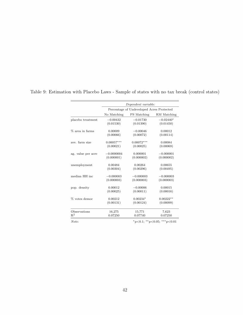
Table 9: Estimation with Placebo Laws - Sample of states with no tax break (control states)

Dependent variable:

Percentage of Undeveloped Acres Protected

No Matching PS Matching RM Matching

placebo treatment −0.00432 −0.01730 −0.02440∗

(0.01530) (0.01390) (0.01450)

% area in farms 0.00009 −0.00046 0.00012(0.00066) (0.00072) (0.00114)

ave. farm size 0.00057∗∗∗ 0.00072∗∗∗ 0.00084(0.00021) (0.00025) (0.00069)

ag. value per acre −0.0000004 0.000001 −0.000001(0.000001) (0.000002) (0.000002)

unemployment 0.00484 0.00264 0.00655(0.00304) (0.00296) (0.00495)

median HH inc −0.000003 −0.000003 −0.000003(0.000003) (0.000003) (0.000003)

pop. density 0.00012 −0.00006 0.00015(0.00025) (0.00011) (0.00016)

% votes democ 0.00212 0.00234∗ 0.00222∗∗

(0.00131) (0.00124) (0.00099)

Observations 16,275 15,771 7,623R2 0.07250 0.07740 0.07250

Note: ∗p<0.1; ∗∗p<0.05; ∗∗∗p<0.01

42

Table 10: Estimation with Placebo Laws - Sample of all states before any tax break

Dependent variable:

Percentage of Undeveloped Acres Protected

No Matching PS Matching RM Matching

placebo treatment 0.02820 0.02870 0.04370∗

(0.02610) (0.02630) (0.02500)

% area in farms −0.00655 −0.00690 −0.00992∗

(0.01290) (0.01300) (0.00516)

ave. farm size 0.00101∗ 0.00107∗ 0.00085(0.00058) (0.00061) (0.00091)

ag. value per acre −0.00003 −0.00003 0.00001∗

(0.00002) (0.00002) (0.00001)

unemployment −0.00248 −0.00262 0.00041(0.00417) (0.00420) (0.00441)

median HH inc 0.000003 0.000003 0.0000001(0.000004) (0.000004) (0.000004)

pop. density 0.00005 0.00005 0.00007(0.00009) (0.00009) (0.00008)

% votes democ −0.00209 −0.00209 0.00039(0.00153) (0.00154) (0.00160)

Observations 10,476 10,368 5,886R2 0.13200 0.13200 0.14700

Note: ∗p<0.1; ∗∗p<0.05; ∗∗∗p<0.01

Table 11: Monte Carlo SimulationRejection Rate for Placebo Laws

Non-corrected St. Errors St. Errors clustered by stateStates that never had Tax Break 0.2576 0.0730

(0.0262) (0.0161)All states before first Tax Break 0.2142 0.0682

(0.0228) (0.0140)

43

7 Appendix

Collapsing data to two effective periods avoid the problem of serially correlated stan-

dard errors. I use a sample of the original data and estimate the effect of five tax breaks

that happen at a specific period in time. I present the equations and some tables for

difference-in-difference estimation.

Before and after difference-in-difference uses a double difference between treated and

control groups, before and after the treatment. I use a yearly average of acres protected

per county, before and after the period 1999-2001, where five states implemented a tax

break incentive6. I define acres before as the average percentage of acres protected in

each county per year, during a period of 8 years between 1991 and 1998, and acres after

is the corresponding percentage of acres protected per year during a same-length period

of time between 2002 and 2009. Some counties do not show any conservation before the

tax break, others do not show conservation after it. In order to avoid positive or negative

biases, I kept all observations: 178 treated and 775 control counties. I present summary

statistics for both samples on Table ??.

Table 12: Summary Statistics - Two Period Data

Group undev prot Prop farm Ave farm agvalue unemploy medhhinc popdens dem

Control

Mean 0.039 0.461 176723 3311 7.55 40052 259 46.30St. Dev. (0.141) (0.294) (136589) (5413) (3.62) (11096) (819) (9.54)

Treated

Mean 0.142 0.245 81131 3693 6.34 44995 604 46.63St. Dev. (0.225) (0.161) (64806) (4259) (3.32) (15858) (1294) (11.19)

I estimate the following equation for a simple difference-in-difference model (Ashen-

6The five states with a tax break in this period are: Connecticut (1999), Delaware (2000), Virginia (2000),Maryland (2001), and South Carolina (2001). I dropped North Carolina (tax break in 1983), and states witha tax break after 2001 but before 2010: Mississippi (2003), Georgia (2006), New York (2007), Iowa (2008),Arkansas (2009) and Florida (2009)

44

felter, 1978, Imbens and Wooldridge 2009)

Yit = α+ γSs + λTt + τ(SsTt) + βXit + εit

where Ss and Tt are group and time dummies, and (SsTt) is the post interaction term.

The second estimation uses a matched sample. I follow the same methods and use

propensity score and mahalanobis distance matrices. I matched on the following observ-

able characteristics before treatment (1998): proportion of acres in farms, agriculture

value per acres, unemployment rate, median household income, population density, per-

centage of votes for democrats in presidential election, proportion of land covered in forest

(1992), percentage of undeveloped land protected until 1998, and average percentage of

undeveloped land protected per year between 1991-1998. The estimated equation is:

Yi = α+ τDi + ∆S(i) + εi

where Yi is the difference in % acres protected before and after treatment, in county i,

and ∆S(i) is a matched-set fixed effect

All specifications indicate that a tax break has a positive and significant effect on

acres protected per county (Table ??). A tax break incentive increases the percentage of

undeveloped land protected per county by year in 0.103% (Propensity Score Matching).

Table 13: Two-Period Difference-in-Difference Results

Dependent variable:

Difference in % of Undeveloped Acres Protected

DID PS RM

treatment 0.106∗∗∗ 0.103∗∗∗ 0.102∗∗∗

(0.018) (0.019) (0.016)

Constant 0.054∗ −0.058 0.074(0.028) (0.055) (0.090)

Observations 953 934 318R2 0.099 0.410 0.508

Note: ∗p<0.1; ∗∗p<0.05; ∗∗∗p<0.01

45