Do Shifts in Labor Shares in Productivity Growth Affect

Eastern Illinois University Eastern Illinois University

The Keep The Keep

Masters Theses Student Theses & Publications

Summer 2020

Do Shifts in Labor Shares in Productivity Growth Affect Poverty Do Shifts in Labor Shares in Productivity Growth Affect Poverty

and Inequality? A Comparative Study of Sub-Saharan Africa and and Inequality? A Comparative Study of Sub-Saharan Africa and

Asia Asia

Precious W. Allor Eastern Illinois University

Follow this and additional works at: https://thekeep.eiu.edu/theses

Part of the Growth and Development Commons, and the Labor Economics Commons

Recommended Citation Recommended Citation Allor, Precious W., "Do Shifts in Labor Shares in Productivity Growth Affect Poverty and Inequality? A Comparative Study of Sub-Saharan Africa and Asia" (2020). Masters Theses. 4812. https://thekeep.eiu.edu/theses/4812

This Dissertation/Thesis is brought to you for free and open access by the Student Theses & Publications at The Keep. It has been accepted for inclusion in Masters Theses by an authorized administrator of The Keep. For more information, please contact [email protected].

https://thekeep.eiu.edu/

https://thekeep.eiu.edu/theses

https://thekeep.eiu.edu/students

https://thekeep.eiu.edu/theses?utm_source=thekeep.eiu.edu%2Ftheses%2F4812&utm_medium=PDF&utm_campaign=PDFCoverPages

http://network.bepress.com/hgg/discipline/346?utm_source=thekeep.eiu.edu%2Ftheses%2F4812&utm_medium=PDF&utm_campaign=PDFCoverPages

http://network.bepress.com/hgg/discipline/349?utm_source=thekeep.eiu.edu%2Ftheses%2F4812&utm_medium=PDF&utm_campaign=PDFCoverPages

https://thekeep.eiu.edu/theses/4812?utm_source=thekeep.eiu.edu%2Ftheses%2F4812&utm_medium=PDF&utm_campaign=PDFCoverPages

mailto:[email protected]

i

Do Shifts in Labor Shares in Productivity Growth affect Poverty and

Inequality?

A Comparative Study of Sub-Saharan Africa and Asia

Precious .W. Allor

[email protected]

Eastern Illinois University

Department of Economics

July 2020

Thesis Committee

Dr. Linda S. Ghent (Chair)

Dr. Ali R. Moshtagh

Dr. Ahmed S. Abou-Zaid

ii

This thesis is submitted in partial fulfillment of the requirements for the award of

a Master’s Degree in Economics at Eastern Illinois University

Copyright © by Precious Allor

All rights reserved

iii

Abstract

This paper examines whether productivity growth induced by intersectoral labor movement

affects inequality and poverty. To address this question a nonparametric shift-share decomposition

technique is employed to decompose productivity growth into the structural change component;

the component of productivity growth that is induced by the intersectoral labor movement, and the

technological change component; the component of productivity growth that is induced by capital

or improvements in productive efficiency. The paper then examines the long-run impact of

structural change-induced productivity growth on poverty and inequality for a sample of 28

countries, and with a focus on Sub-saharan Africa and Asia. The Theil index of industrial wage

inequality and the Gini coefficient from the estimated household income inequality data from the

University of Texas Inequality Project (UTIP) are used as measures of inequality, and the

percentage change in household final consumption measures poverty. Parametric fixed effects

estimation techniques are employed and I find that labor share in productivity growth reduces

poverty and inequality for the full sample and the Asia and sub-Saharan Africa subsamples. The

effects are however stronger for Asia than for sub-Saharan Africa. Nonparametric time-varying

coefficient estimation techniques are also employed to determine if any nonlinearities exist in the

relationship between the dependent and independent variables. The results confirm that structural

change has nonlinear effects on poverty and inequality. The paper recommends that governments

should encourage policies directed towards improving labor shares in productivity as a means to

reduce poverty and inequality, especially for developing countries.

Keywords: Structural change, industrial wage, inequality, productivity, nonparametric

iv

Acknowledgment

I praise the Almighty God for His abundant mercies, knowledge, wisdom, and strength that

have guided me to the successful completion of this thesis. I wish to profoundly acknowledge and

thank Dr. Linda S. Ghent for supervising this project. Your input into this project ensured its

successful completion. I also thank Dr. Ahmed S. Abou-Zaid and Dr. Ali R. Mostagh for serving

on my committee and for their input.

I wish to also acknowledge the significant contribution of Mr. Ahmed Salim Nuhu, who

served as my mentor throughout this project. I also wish to thank the entire faculty of the

Department of Economics of Eastern Illinois University for all the support and guidance that has

shaped me into a better person intellectually and otherwise. Lastly, I thank all my friends for the

support and encouragement they offered on this successful journey. God bless you all.

v

Dedication

I dedicate this work to my ever-loving mother, Comfort Lamisi Awemoni, my Uncle Mr. Luguje

Micheal, and the GNPC Foundation, Ghana

vi

Table of Contents

Abstract ......................................................................................................................................... iii

Acknowledgment .......................................................................................................................... iv

Dedication ...................................................................................................................................... v

List of Tables .............................................................................................................................. viii

List of Figures ............................................................................................................................... ix

Chapter One .................................................................................................................................. 1

1.1 BACKGROUND .............................................................................................................................................. 1 1.2 PROBLEM STATEMENT ................................................................................................................................ 3 1.3 OBJECTIVES/RESEARCH QUESTIONS ......................................................................................................... 5 1.4 SIGNIFICANCE OF THE STUDY. .................................................................................................................... 6 1.5 SCOPE AND ORGANIZATION OF THE STUDY ............................................................................................... 7

Chapter Two .................................................................................................................................. 8

LITERATURE REVIEW .............................................................................................................................................. 8 2.1 Structural Change ....................................................................................................................................... 8 2.2 Poverty and Inequality ............................................................................................................................... 13 2.3 Structural Change and Inequality ............................................................................................................. 15

Chapter Three ............................................................................................................................. 20

DATA AND METHODOLOGY.................................................................................................................................... 20 3.1. DATA .......................................................................................................................................................... 20 3.2 VARIABLE DESCRIPTION ........................................................................................................................... 21

3.2.1 Inequality and Poverty. ......................................................................................................................... 21 3.2.2 Structural Change ................................................................................................................................. 22 3.2.3 Other Covariates ................................................................................................................................... 22

3.3 DECOMPOSITION OF PRODUCTIVITY GROWTH ....................................................................................... 24 3.4 ESTIMATION PROCEDURE. ........................................................................................................................ 26

3.4.1 Parametric Methods .............................................................................................................................. 26 3.4.2 Nonparametric Dimension. .................................................................................................................. 28

Chapter Four ............................................................................................................................... 31

4.1 TRENDS IN EMPLOYMENT SHARES .................................................................................................................. 31 4.2 AGRICULTURAL EMPLOYMENT SHARES AND INEQUALITY .......................................................................... 34 4.3 DESCRIPTIVE STATISTICS .............................................................................................................................. 37

Chapter Five ................................................................................................................................ 41

Estimation Results ...................................................................................................................... 41

5.1 PARAMETRIC ESTIMATION RESULTS............................................................................................................ 41

vii

5.1.1 Industrial Wage Inequality ....................................................................................................................... 42 5.1.2 Income Inequality ................................................................................................................................. 48 5.1.3 Poverty ................................................................................................................................................... 53

5.2 NON-PARAMETRIC ESTIMATIONS ................................................................................................................. 58 5.2.1 Industrial Wage Inequality .................................................................................................................. 59 5.2.2 Income Inequality ................................................................................................................................. 63 5.2.3 Poverty ................................................................................................................................................... 66

Chapter Six .................................................................................................................................. 70

6.1 SUMMARY AND FINDINGS .............................................................................................................................. 70 6.2 RECOMMENDATIONS. ................................................................................................................................ 73 6.3 LIMITATIONS ............................................................................................................................................. 74

References .................................................................................................................................... 75

viii

List of Tables

Table 1: Summary Statistics ......................................................................................................... 39

Table 2:Structural Change and Industrial Wage Inequality- Full Sample .................................... 42

Table 3: Structural Change and Industrial Wage Inequality-SSA Subsample ............................. 45

Table 4: Structural Change and Industrial Wage Inequality-Asia Subsample ............................ 47

Table 5: Structural Change and Income Inequality: Full Sample ................................................. 49

Table 6: Structural Change and Income Inequality: SSA Subsample .......................................... 51

Table 7: Structural Change and Income Inequality: Asia Subsample .......................................... 52

Table 8: Structural Change and Poverty: Full Sample ................................................................. 54

Table 9: Structural Change and Poverty: SSA Subsample ........................................................... 56

Table 10: Structural Change and Poverty: Asia Subsample ........................................................ 57

ix

List of Figures

Figure 1: Agricultural and Manufacturing Shares in Employment .............................................. 32

Figure 2: Agricultural and Services Shares in Employment ......................................................... 32

Figure 3: Agricultural Employment Share and Productivity (SSA) ............................................. 33

Figure 4: Agricultural Employment Share and Productivity (Asia) ............................................. 33

Figure 5: Agricultural Employment Share and Sectoral Wage Inequality .................................. 34

Figure 6: Income Inequality and Agricultural Employment Share ............................................... 35

Figure 7: Globalization and Industrial Wage Inequality............................................................... 36

Figure 8: Globalization and Income Inequality ............................................................................ 37

Figure 9: Non-Linear Time-Varying Coefficients- Industrial Wage Inequality- Full Sample ..... 59

Figure 10: Non-Linear Time-Varying Coefficients -Industrial wage inequality: SSA Subsample

....................................................................................................................................................... 61

Figure 11: Non-Linear Time-Varying Coefficients- Industrial wage inequality: ASIA Subsample

....................................................................................................................................................... 62

Figure 12: Non-Linear Time-Varying Coefficients - Income Inequality: Full Sample ............... 64

Figure 13: Non-Linear Time-Varying Coefficients – Income Inequality: SSA Subsample ......... 64

Figure 14: Non-Linear Time-Varying Coefficients - Income Inequality: Asian Subsample ....... 65

Figure 15: Non-Linear Time-Varying Coefficients - Poverty: Full Sample ................................. 67

Figure 16: Non-Linear Time-Varying Coefficients - Poverty: SSA Subsample .......................... 68

Table 17: Non-Linear Time-Varying Coefficients - Poverty: Asian Subsample ......................... 68

1

Chapter One

1.1 Background

The last decade has seen a significant rise in world GDP growth. Most importantly, the

recent decade has been characterized by a significant surge in the economic growth of developing

countries. This has brought the study of economic growth and structural change to the forefront of

recent research. Economic growth is viewed as a tool for the improvement of the standard of living

and in the general welfare of society. This growth can be a result of both technological change and

changes in labor productivity as workers move from one sector of the economy to another (which

will be referred to as a change in the labor share of productivity growth). The world bank reports

growth rates of 2.3 percent for sub-Saharan Africa, 6.3 percent for East Asia, and about 2 percent

for Latin America. Much of the growth of these economies has been attributed to the structural

transformations of these countries. A gradual shift from the agricultural sector towards

manufacturing, and much recently the service sector has led to a significant improvement in

productivity and hence economic growth. The recent technological surge and increased

globalization have made the effect of structural change even more eminent.

Structural change refers to the reallocation of resources or factors of production from one

sector of the economy to the other as the economy transforms overtime. This concept of structural

change and inter-sectoral labor movement can be traced back to the Lewis-dual sector model

(Lewis, 1954). This model generally assumes a two-sector economy where one sector is

industrialized and the other sector is agricultural. Other ways of describing the sectors will be

formal and informal or urban and rural (Fields, 2004). Differences in labor productivity and wages

across sectors results in the movement of labor. Typically, labor moves away from the agricultural

sector which has lower marginal productivity to other sectors with higher marginal productivity.

2

These movements affect the marginal productivity of both sectors and hence output. Economic

theory suggests that such movements will continue until marginal productivity is equalized across

sectors. In this sense, structural change is mostly measured by looking at the changes in labor

shares in productivity or employment across different sectors of the economy.

Even though structural change is generally viewed through the lens of economics, a much

broader view of structural change will involve a look at the changes in the entire structure of the

economy. This is the position taken by Kuznets (1965). He argues that structural change should be

viewed more broadly as changes in the entire structure of society, including changes in its social

and political institutions and its belief systems.

From whichever way structural change is viewed, the evidence of the effect of structural

change on economic growth is clear. A plethora of studies has examined the effect of structural

change on economic growth. Li et al (2016), for instance, find that technological change and

movement of labor generally spurs economic growth. They argue that the effect of the labor

movement will depend on the direction of movement. If labor typically moves from less-

productive to more-productive sectors of the economy, it will positively affect economic growth.

The reverse is true as well if labor moves from more-productive to less-productive areas. In line

with this, Carmignani & Mandeville (2014) argue that structural change in Africa has been without

industrialization. The decline in agriculture in Africa has not been coupled with a rise in

manufacturing, but a rise in the service sector instead, which is less productive. Hence, they argue

that structural change in Africa has not had a significant impact on economic growth. Peneder

(2002) also finds that structural change has both positive and negative effects on economic growth.

He argues that when the two effects are netted out, structural change does not appear to have a

strong effect on economic growth.

3

Despite the recent surge in economic growth in developing countries, poverty and

inequality have not seen any significant improvements. The recent advent of structural change has

gone alongside rising inequality levels. For instance, after 1990, Asia has generally experienced

rising levels of income inequality, despite the surge in technological progress (Jain-Chandra et al

2016). The United Nations Development Program (UNDP) 2017 report on inequality in Sub-

Saharan Africa (SSA) also states that SSA is still the most unequal region globally, with 10 out of

the 19 most unequal countries in the world coming from the region. This is despite the high rate

of structural change ongoing in the region. This problem casts doubt on the factors driving the

recent economic growth of developing countries, and the translation of higher economic growth

rates into improvement in social welfare.

1.2 Problem Statement

The relationship between structural change and inequality is embodied in the Kuznets

hypothesis. Kuznets (1955) puts forward an inverted “U-shaped” relationship between economic

growth and income inequality. He states that income inequality initially rises as an economy

grows, but eventually decreases after a certain point in the economic transformation of the country.

This relationship is due to the reallocation of labor employment from the agriculture sector to other

sectors as the economy progresses. The initial rise in inequality is due to the difference in incomes

between the agricultural sector and the other sectors which are assumed to be more modified.

However, as more people move into the modern sectors, the productivity of the agricultural sector

will eventually rise as fewer people are now employed there. This then results in decreasing

inequality. Other schools of thought are of the view that inequality is an unavoidable consequence

of economic growth and should not be an issue of much concern, as long as growth is maximized

and poverty is minimized. However, it is mostly argued that countries can sustain economic growth

4

while minimizing poverty and inequality. This is the position of the UNDP in its 2014 report on

inequality in developing countries. (Hub, n.d.)

As economies are moving from agrarian economies to manufacturing, and service-based

economies, labor shares in productivity have declined significantly. Karabarbounis & Neiman

(2012) argue that the significant fall in labor shares over the past 30 years is due to the rise in

corporate savings. Barkai (2016) also argues that this decline in labor shares has not been

consolidated by a rise in capital shares. There rather appears to be a significant rise in profit shares,

especially in the U.S non-financial corporate sector. Rodrik (1997) blames this decline in labor

shares on globalization. He argues that globalization has improved the mobility of capital. This

increased mobility has led to increased opportunities outside and has given the power to capitalists

to bargain for lower wages. Beqiraj et al (2018) also attribute the decline in labor shares to the

growing service sector compared to the manufacturing and agricultural sectors. They argue that,

because the service sector wage share is relatively low, the growth of the service sector at the

expense of the manufacturing and agricultural sectors reduces the aggregate wage share.

Most authors argue that structural change affects inequality through its effect on factor

shares of the various sectors of the economy. Hence authors have often measured structural change

using sectoral factor shares. In their study on the impact of structural change on inequality, Roy &

Roy (2017) measure inequality using manufacturing and service sector shares in GDP. Dartanto et

al (2016) also measure structural change by considering sector labor shares in GDP. A concern

with the use of only factor shares is the failure to consider the productivity of factors across sectors.

5

The productivity of factors in the various sectors is significant for economic growth and hence

inequality and poverty reduction.

Again, authors have mostly assumed some form of a parametric relationship between

structural change and inequality. Pre-imposing a specific functional relationship to a model has

the possibility of excluding information. This can result in a model misspecification problem that

tends to bias the estimates. Nonparametric methods are not popular in the literature on this subject,

but they are significant tools in tracing the actual functional form or nature of the relationship

between structural change, poverty, and inequality.

Broadening the analysis by looking at shifts in factor shares in productivity and the

implications for poverty and inequality will be more informative. It will be intuitive to understand

the extent to which the growing inequality and poverty in developing countries can be attributed

to the recent decline in labor shares in productivity growth.

1.3 Objectives/Research Questions

The study will seek to determine the extent to which shifts in labor shares in productivity

affect poverty and inequality. Specific questions that this study will attempt to answer are:

1. What are the effects of shifts in labor shares in productivity on poverty and

inequality in general?

2. Do these effects differ for Sub-Saharan Africa and Asia?

3. Are there any non-linearities in these relationships over time?

6

1.4 Significance of the Study.

There exist a lot of literature on the effect of structural change on labor shares and economic

growth. There are a few other studies that have linked structural changes to inequality. However,

most of these papers have measured structural change using sector shares in output. Not many of

these studies have used labor share in productivity as a measure of structural change. A notable

study that uses this measurement is Andersson & Palacio (2017), who use labor productivity

growth to study income inequality and agricultural development of Latin America. The study will

broaden the literature in this area by applying a similar methodology to understand the effect of

shifts in labor shares in productivity on poverty and inequality, with a focus on sub-Saharan Africa

and Asia

Extending the analysis by applying nonparametric techniques, is a trajectory that is not

taken by any known study in this area. This is an attempt to reveal the actual functional form of

the relationships between structural change, inequality, and poverty. This procedure will possibly

reveal information about these relationships that will otherwise be obscured by using a pre-

determined functional form.

A study into the effect of labor shares in productivity on poverty and inequality will explain

the current trend we see of a rise in inequality and poverty in the face of structural change in many

developing countries. A comparison across geographic regions will also allow us to understand

regional differences that may exist and how these differences affect the relationship between labor

shares in productivity, poverty, and inequality. This will make this study more comprehensive and

informative for both theoretical and policy-making purposes.

7

1.5 Scope and Organization of the Study

The study will employ panel data for a sample of 28 countries from Europe, Latin America,

Sub-Saharan Africa, and Asia. The data spans the period from 1963 to 2012. Four main data

sources will be employed: The Groningen Growth and Development Center (GGDC) 10-sector

database, Groningen Growth and Development Center (GGDC) Penn-World Tables, The

University of Texas Inequality Project (UTIP) database, and the Worldbank Development

Indicators (WDI) database. The rest of the study continues as follows.

Chapter 2 presents a literature review of the theories and empirical studies on structural

change, poverty, and inequality. Chapter 3 presents the data and variable descriptions along with

the empirical methodology and estimation techniques. Chapter 4 presents detailed descriptive

statistics and trend analysis on structural change, poverty, and inequality. Chapter 5 presents

estimation results and interpretation of results. Chapter 6 concludes the study with a summary of

findings, recommendations, and limitations.

8

Chapter Two

Literature Review

2.1 Structural Change

Structural change can be considered as the central theme of development economics. The

study of structural change has been approached from either a micro or a macro perspective.

Structural change from the micro perspective focuses on issues such as the functioning of

economies, their markets, institutions, and the mechanisms for resource allocation. This approach

concentrates on the micro-level analysis of individual units rather than any focus on historical

transformations. From a broader perspective, structural change is the long-run process of

transformation of economic structures which results in economic growth. This involves economy-

wide changes such as industrialization, urbanization, globalization, technological change, and

transformation of the agricultural sector. Kuznets identifies these as elements of modern economic

growth. This approach relies on the historical development of societies (Syrquin, 1988).

Structural change can also be studied as the relative importance of various sectors of the

economy as the economy transforms over time. Industrialization then becomes the central theme

of structural change. Relative sector performance can then be measured by considering either

productivity levels or factor reallocations across these sectors. Structural change studied as a shift

in factor allocations can be attributed to theories such as the Rostow’s stages of growth theory and

Lewis dual-sector theory.

Rostow (1971) outlines five stages in the development and transformation of society. The

first stage is the traditional stage where the economy is primitive. Subsistence agriculture and

barter are predominant in this stage. The second stage is the transitional stage or the preconditions

for take-off, where the economy accumulates both physical and human capital. The economy then

9

takes off into development through industrialization and increased investment. This stage is

characterized by economic growth and some changes in the political structure of the economy. The

economy then drives to maturity through diversification, innovation, and less reliance on imports.

The last stage is the stage of mass consumption where the economy shifts towards the consumption

of durable goods. The economy becomes service-oriented at this stage. This theory considers

structural change to be attributed to the accumulation of capital for take-off. The Clark-Fisher

model also predicts a shift from the agricultural sector to the manufacturing sector and then to the

service sector as the economy progresses (Clark, 1957).

The Lewis (1954) dual-sector model is the basis for studies on factor reallocation across

sectors of the economy. Differences in the marginal productivity of different sectors drive

movements across these sectors. Labor typically moves from sectors with relatively low marginal

productivity to sectors with high marginal productivity. A dual-sector economy is assumed with

the agricultural sector mostly considered to be the less productive sector. Labor will move from

the agricultural sector to the industrial sector. These movements reduce the marginal productivity

of labor in the industrial sector and increase that of the agricultural sector. This continues until the

marginal productivities of labor, and hence wages are equalized across sectors. These factor

reallocations promote economic growth because resources get allocated to areas where they are

most relevant.

The major themes in structural change are globalization, technological change, and shifts

in factor shares. Even though this paper will measure structural change as shifts in labor shares in

productivity, it is important to view structural change more broadly to cover globalization and

technological change. Kuznets (1965) argues further that structural change should be viewed even

10

more broadly to include changes in the entire structure of society. This includes changes in the

economic, social, political institutions, and the belief systems of society.

The growth impact of these labor allocation will depend on the direction of the movement

of labor. McMillan & Rodrik (2011) argue that structural change will be growth-enhancing if labor

moves from less productive to more productive sectors. They find such a pattern for Asian

countries. However, if labor typically moves from more productive sectors to less productive

sectors, structural change will be growth-reducing. They argue that this is the case for Latin

American and African countries. Akkemik (2005) studies the impact of shifts of labor across

sectors on aggregate productivity growth for Singapore from 1965 to 2002. His results show that

shifts in labor share increased productivity, especially for the manufacturing sector in the 1985 era

when the government pursued interventionist policies. However, the impact was negative during

the era of labor market liberalization.

In a comparative study of productivity growth, technological growth, and structural

change, Fagerberg (2000) uses a sample of 39 countries and 24 industries between 1973 to 1990

to examine this point further. He finds that on average, structural change has not been growth-

enhancing. Peneder (2002) also finds that structural change has both positive and negative effects

on economic growth. He argues that these effects net out, hence structural changes have a weak

effect on economic growth. In studying structural change and total productivity growth in China,

Chen et al (2011) measure structural change by decomposing productivity growth due to factor

reallocation. Their results show that structural change positively impacts total factor productivity

growth.

Examining structural change within the framework of Engel’s Law, Laitner (2000) finds

that structural change enhances economic growth. He designs a model with agriculture and

11

industry as the only sectors. Agriculture makes use of land. At the early stages of growth,

consumption is important and therefore the land becomes very valuable. This implies that land will

constitute a greater portion of capital accumulation. The paper argues that if structural changes

result in increased incomes overtime, Engel’s law will predict that demand will shift towards

manufactured goods. This diminishes the value of land relative to reproducible capital. This also

increases the value of the product section of the national accounts and hence economic growth.

Using a multi-sector model of economic growth, Li et al. (2016) analyze the relationship

between structural change and economic growth. Sectors are assumed to have different rates of

technological progress. This implies differences in wages and revenues across sectors. The model

also regards labor movements as an endogenous revenue maximization decision, implying that

labor moves out of the basic sectors to advanced sectors. The conclusion is that labor moving from

basic sectors to advanced sectors enhances aggregate economic growth. In tracing the sources of

the rapid economic growth of China, Fan et al (2003) extend the Solow growth model to include

a measure of structural change. Their results show that structural change played a significant role

in enhancing economic growth through the reallocation of resources from low-productivity areas

to high-productivity areas. The interaction between human capital, structural change, and

economic growth is studied by Teixeira & Queirós (2016). They find that the interaction between

human capital and structural change, especially for knowledge-intensive sectors is growth-

enhancing.

A new measure of structural change called the effective structural change index (ESC) is

introduced by Vu (2017). He applies this to study the effects of structural change on productivity

for 19 Asian countries from 1970 to 2012. The paper finds a positive effect of structural change

on productivity and growth. A dynamic general equilibrium method is used by Echevarria (1997)

12

to study the role of sectoral composition in economic growth. He adopts a typical Solow model

of sustained growth with multiple consumption goods. The study establishes that there is a

bidirectional relationship between sectoral composition and economic growth.

In studying the impact of economic globalization on economic growth in the Organization

of Islamic Cooperation (OIC) countries, Samimi & Jenatabadi (2014) apply the Generalized

Method of Moments procedures. The study establishes that globalization has a positive effect on

economic growth. However, the effect is stronger in countries with better educational systems and

well-functioning financial systems. In a similar way, Ying, Chang, & Lee, (2014) explore the

impact of globalization on economic growth for the Association of Southeast Asian Nations

(ASEAN) between 1970 to 2008. Globalization is divided into economic, social, and political

aspects. Their results establish that economic globalization enhances economic growth while

social globalization impedes it. Political globalization has no significant effect on economic

growth. A similar methodology is applied by Kilic (2015) in assessing the impact of globalization

on economic growth for a panel of 74 developing countries between 1981 to 2011. Results

establish a positive effect of economic and political globalization on economic growth while social

globalization has a negative effect.

Irrespective of how structural change is examined, the literature strongly establishes the

important role of structural change in spurring economic growth. It is, however, important to

extend the analysis to understanding if structural change affects the actual welfare of people.

Understanding how shifts in sector labor shares in productivity affect poverty and inequality will

broaden the discussion on the true effect of structural change. This forms the basis for this paper.

13

2.2 Poverty and Inequality

One of the major targets of the Sustainable Development Goals is the reduction in

inequality, either within countries or between them. Despite the fall in other forms of inequalities,

income inequality is still persistent in most developing countries even in the presence of economic

growth (Klasen et al, 2016). One of the most significant consequences of the industrial revolution

was the rise in inter-country inequality. Over the years, however, global inequality has been

roughly stable and, in some cases, falling gradually, while there appears to be growing intra-

country inequality, especially in developing countries.

In assessing the changing trends of world inequality between the 1960s and the 1970s,

Schultz (1998) finds that about two-thirds of the measure of inequality is inter-country while three-

tenths is within-country. However, the study points out that studying world inequality is a

cumbersome process and will require better data. Similarly, Goesling (2001) provides evidence

that suggests a changing trend in world inequality between the 1980s and the 1990s. As inter-

country inequality is significantly falling, within-country inequality is significantly widening.

Focusing on developing countries, Ravallion (2014) identifies that, income inequality in the

developing world has seen a steady decline over the past 30 years. This is due to reductions in the

inequality between countries. However, within-country inequality has been rising slowly.

Technological change is one of the drivers of inequality. While technology has led to

improvements in productivity, it has also raised the returns to capital and skilled labor and hence

widened the wage inequality gap (Dabla-Norris et al, 2015). Globalization has also been blamed

for the rising inequality levels. Inequalities in labor earnings between skilled and unskilled labor

are becoming more profound, especially in developing countries where unskilled labor and the

14

informal sector are still significantly large. Williamson, (1997) asserts that between one-third and

one- half of the inequality in the USA and the OECD countries could be attributed to globalization.

In contributing to the debate on the resurgence of inequality in some advanced societies,

Alderson & Nielsen (2002) suggest that variations in inequality could be associated with the

percentage of people in the agricultural sector which is significantly underperforming. They also

identify institutional factors such as union density and decommodification as contributing to

income inequality.

The literature on inequality in Africa emphasizes growing levels of inequality in Sub-

Saharan Africa. The recent global world report by Credit Suisse (2014) identifies Southern Africa

as the most unequal sub-region, followed by Central Africa and West Africa. East and North Africa

have the lowest income inequality in Africa. However, in comparison to the world, they still lag.

The report further states that income in Africa is highly concentrated, with the top 10 percent

controlling about 78 percent of the entire wealth in the continent. This pattern is not too different

for other continents.

Looking at poverty and inequality in Asia, Kanbur (2013) argues that Asia has reduced

poverty faster than any other region in the past two decades. However, the region has also

experienced growing levels of inequality. The paper also identifies that technological change,

globalization, and market-oriented reforms, are responsible for the surge in the economic growth

of the region, but they are also responsible for the growing levels of inequality.

The literature on the relationship between economic growth and income inequality can be

broadly divided into two strands. Lewis and Kuznets believe that there appears to be some form

of a mechanical relationship between the two. At the early stages of development, faster economic

15

growth results in higher inequality. This reflects the Kuznets curve, where at the initial stages of

the economic transformation of a country, higher economic growth results in higher levels of

inequality. Inequality eventually decreases as the economy progresses and undergoes

industrialization (Kuznets, 1965). This change is due to the reallocation of labor from the

agricultural sector to the industrial sector. Barro (1999) emphasizes that the Kuznets curve theory

appears to be an empirical regularity when tracing the growth path of countries. He finds evidence

to show that high levels of inequality reduces growth in relatively poor countries but encourages

growth in relatively rich countries.

The other strand of that literature has attempted to determine the causal factors of growth

and inequality independently. Barro & Sala-i-Martin (1995) look at growth independently of

inequality while Li et al (2016) study inequality independently.

However, Lundberg & Squire (2003) study growth and inequality simultaneously and

conclude that the determinants of economic growth and inequality cannot be considered mutually

exclusive. Understanding the factors behind the rising inequality in the face of higher economic

growth will require a better understanding of the factors driving economic growth and their

impacts on inequality. One such factor is structural change.

2.3 Structural Change and Inequality

The relationship between structural changes and income inequality is an area that has not

been greatly explored in the economic literature. Trade, foreign direct investment, globalization,

and factor shares are among the several ways that structural change is considered by economists.

Structural change has implications for factor shares in an economy. For example, movements of

labor from less productive to more productive areas increases labor productivity and labor shares

16

significantly, which has effects on poverty and inequality. Following the Lewis dual-sector model,

the movement of labor from the agricultural sector (where marginal productivity of labor is low)

to the industrial sector (where marginal productivity of labor is high) will increase the return to

labor across sectors. This implies higher incomes for workers which would then be expected to

translate into lower levels of inequality. The Kuznets hypothesis argues that at the initial stages of

structural transformation, the movement of labor from the agricultural sector to other sectors

reduces the agricultural employment and GDP shares, without any significant increase in

productivity. Hence, inter-sector inequality is likely to be widened initially. Over time, this gap

begins to close as productivity levels rise (Andersson & Palacio, 2017).

The conclusion of Kuznets (1955) that structural transformation widens inequality can be

described as comprising two major sub-processes. The first sub-process is inter-sector inequality,

which involves the movement of labor from sectors with low mean income to sectors with high

mean income. The second process is within-sector inequality which involves movement from

sectors with low variance in incomes to sectors with higher variance in incomes. Kuznets argues

that if both sub-processes move in the same direction, then inequality will unambiguously increase.

However, if the movements are in opposite directions, the effect on inequality is ambiguous.

Baymul & Sen (2018) argue that the movement of labor from agriculture to manufacturing

unambiguously decreases inequality while movement from agriculture to the service sector

unambiguously increases inequality. These effects exist irrespective of the stage of structural

transformation of the country. This finding seems to agree with Vries et al (2014) who conclude

that the movement of labor from agriculture to the service sectors is not growth-enhancing. In their

study on structural transformation and inequality in Africa, Bolt et al (2017) find similar results.

They find that increases in the share of employment in the agriculture and industry sectors decrease

17

average inequality in Africa, while the increase in the employment share in the service sector

increases inequality.

Using the University of Texas Inequality Project (UTIP), Kum (2008) presents data on

inequality in manufacturing pay structures from 1963 to 2002. The paper measures structural

change by considering changes in employment shares of the agricultural, manufacturing, and

service sectors. The paper finds that movement out of the agricultural sector increases the

variability of inequality in manufacturing-sector pay.

The lack of consensus on the empirical evidence of the Kuznets curve is pointed out by

Paul (2016). He argues that heterogeneities existing in the composition of structural transformation

across income distributions explain the empirical irregularities. He further argues that the gap

between the agricultural and non-agricultural sectors and the differences in the rate of structural

transformation across income quantiles jointly determine the direction of motion on the Kuznets

curve. He adds that the effect of structural transformation on inequality depends on the variation

of earning ratios across income quantiles.

In their study on structural change and inequality in Indonesia, Dartanto et al (2016) find

that the movement of labor from agriculture to service sectors, the rural to urban centers, and from

informal sectors to formal sectors widens the inequality gap in Indonesia. Wan et al (2016) also

find that structural changes have contributed significantly to the rising levels of inequality in

China. Zhu & Trefler (2005) argue that structural change widens the gap in the return to earnings

between low skills and high skills. They add that developing countries that experience high wage

inequalities are those whose export shares are oriented towards skill-intensive goods.

In their analysis of the trend of structural change in Asia, Park et al (2014) conclude that

much of the recent surge in the economic growth of Asia can be attributed to major structural

18

changes in the Asian economies. However, they emphasize that the ongoing structural change has

impinged on inequality, even though the effect differs for each country. They conclude that

inequality is a result of adjustment costs associated with structural changes which if tackled could

mitigate the level of inequality observed in the region. In the long-term, structural change is

expected to reduce inequality through the creation of new job opportunities. However, in the short-

run, structural change worsens inequality as it shifts demand away from unskilled labor towards

skilled labor.

The impact of structural change on income inequality is also studied by Roy & Roy (2017)

for a sample of 217 countries for the period 1991 to 2014. The study measures structural change

by using the shares of manufacturing and service sectors in GDP. They find that growth in these

factor-shares worsens inequality. Jacobson & Occhino (2012), also study the effect of declining

labor shares on inequality in the United States. They argue that inequality mostly increases when

labor shares decline and capital shares rise. Their findings confirm that a decrease in labor shares

increase inequality measured by the Gini index. Signor et al, (2019) explore similar relationships

for Brazil. They study the determinants of income inequality in Brazil. They also show that much

of the increase in income inequality can be attributed to declining labor incomes across different

ethnic groups.

The impact of globalization on wage inequality is also studied by Yay et al (2016) for a

sample of 90 developed and developing countries for the period 1970 to 2005. Globalization is

measured using the Konjunkturforschungsstelle (KOF) globalization index and the Economic

Freedom Index by the Fraser Institute. Wage inequality is measured using the Theil industrial pay

19

inequality index by the University of Texas Inequality Project. They find that globalization and

deregulation contribute significantly to wage inequality.

The impact of globalization on inequality is also studied by Dreher & Gaston (2008) using

measures of industrial wage inequality and household inequality measures. They capture the

economic, social, and political dimensions of globalization. They establish that globalization

significantly exacerbates inequality. In their study on globalization, financial depth, and inequality

in sub-Saharan Africa, Kai & Hamori (2009) also confirm that globalization aggravates inequality

in the region. They also argue that the extent of the effect depends on the level of development of

the country. In their study on the impact of globalization on inequality in Latin America, Nissanke

& Thorbecke, (2010) also agree that the impact of globalization on poverty and inequality is

context-specific and will depend greatly on country-specific conditions.

In analyzing the impact of structural change on poverty and inequality, most authors

usually argue that structural change affects inequality through its effects on factors shares. Hence

changes in factor shares have been used by most authors in doing this analysis. This paper

concentrates specifically on changes in labor shares in productivity. Labor shares in productivity

have been significantly declining in recent times (Grossman et al (2017). Research by Bengtsson

& Waldenström, (2018) and Piketty (2015) have associated the rising levels of inequality to this

phenomenon of declining labor shares in productivity. This paper will contribute to this literature

by empirically testing how changes in labor shares in productivity growth affect poverty and

inequality. Focusing on Asia, and Sub-Sharan Africa will provide a wider perspective on region-

specific differences in these effects.

20

Chapter Three

Data and Methodology

3.1. Data

The study employs panel data for 28 countries from Europe, Latin America, Sub-Saharan

Africa, and Asia. This comprises seven European Countries, seven Asian countries, four Latin

American countries, and ten Sub-Saharan African countries. The dataset spans the years 1963 to

2012, and as much data as its available during this period is collected for each country. Four main

data sources are employed: the Groningen Growth and Development Center (GGDC) 10-sector

database, the Groningen Growth and Development Center (GGDC) Penn-World Tables, the

University of Texas Inequality Project (UTIP) database, and the World Bank Development

Indicators (WDI) database.

The GGDC 10-sector based data contains information on value-added at current national

prices (in millions), value-added at constant national prices (in millions), and employment shares

(in thousands) for 10 sectors of the economy for each country. The 10 sectors are agriculture;

mining; utilities; manufacturing; construction; trade, restaurants, and hotels; transport, storage, and

communication; fire, insurance, and services; government services; and community, social, and

personal services.

The University of Texas Inequality project database contains two measures of inequality

that are utilized for this study. The Penn World Table and the WDI databases contain

macroeconomic data for all countries.

21

3.2 Variable Description

3.2.1 Inequality and Poverty.

To measure inequality, two main variables are extracted from the UTIP database; Industrial

wage inequality data and the Estimated Household Income inequality dataset (EHII). Wage

inequality is a global Theil index of industrial wage inequality computed for about 151 countries.

The Theil index computations are done based on the United Nations Industrial Development

Organization (UNIDO) industrial statistics. The Theil indices are a better measure of inequality

than standard measures because of their decomposability. Inequality can be decomposed based on

dimensions such as population groups or income sources. The Theil’s index is generally presented

as:

T =1

𝑛∑

𝑦𝑖𝜇

𝑛

𝑖=0

ln (𝑦𝑖𝜇) (1)

Where n is the population, yi is the income of group i, and µ is the mean income. The

measure is increasing in inequality starting from 𝑇 = 0 where the group income is equal to the

mean income (𝑦𝑖 = 𝜇).

Household income inequality is measured using the Gini coefficient data provided in the

EHII. This Gini coefficient measure is derived from a regression function with the World Bank’s

Deininger & Squire (1996) Gini coefficient measure as the dependent variable. The independent

variables are the industrial wage inequality and other covariates contained in the World Bank’s

Deininger & Squire (1996) dataset such as; the share of manufacturing employment in total

population, the type of Gini measure involved (whether the measure is gross or net of taxes),

household or personal income, and whether the Gini is an income or expenditure measure

22

(Galbraith et al, 2015). The Gini coefficient in this data is computed by using the coefficients from

this regression.

Poverty is measured using the percentage change in household final consumption

expenditure per capita from one year to another. This is computed from Household final

expenditure per capita in constant 2010 dollars extracted from the WDI database. A positive

percentage change implies a reduction in poverty. This variable may be a relatively weak measure

of the poverty rate, but due to data unavailability for other variables such as the poverty headcount

ratio, it is preferred. Visaria (1981) also uses household expenditure per capita as a measure of

poverty in studying poverty and unemployment in India.

3.2.2 Structural Change

Structural change is measured as productivity growth induced by intersectoral movement

of labor. This is done using a decomposition process suggested by McMillan & Rodrik (2011).

The procedure is set out in the methodology section of this chapter. The decomposition process is

done by utilizing the GGDC 10-sector data. This becomes the independent variable of focus for

the study and will be expected to have a negative relationship with the industrial wage inequality

and the income inequality variable but it is expected to have a positive relationship with the

percentage change in household final expenditure per capita.

3.2.3 Other Covariates

This study also controls for trade openness. This is used to capture the effect of

globalization on inequality. Data on trade openness are taken from the WDI database. This is

measured as trade as a percentage of GDP. Open trade is expected to positively impact GDP

growth which theoretically should reduce poverty and inequality. The population growth rate is

also controlled for in the estimations. The data are also derived from the WDI database. The

23

increasing population is expected to worsen poverty and inequality. Ahlburg (1996), argues that

population growth is likely to reduce per capita income which in turn increases poverty and reduces

welfare.

Real GDP per capita is used as a proxy for income. GDP per capita in constant 2011

international dollars is used. This is also derived from the WDI database. The log of real GDP per

capita is used in this analysis. A squared term is also added to capture any nonlinearities in how

income affects poverty and inequality. It is expected that increased income per capita leads to a

reduction in poverty and inequality generally. However, following the Kuznets hypothesis,

developing countries are expected to initially have increased inequality as the economy grows.

However, this trend is expected to be reversed after a point in the transformation of the economy.

Hence, the coefficient on the log of GDP per capita is expected to have a positive sign while the

coefficient on the squared term of the log of GDP will be negative for measures of inequality.

The estimation also controls for the unemployment rate. The International Labor

Organization (ILO) estimate of the unemployment rate as a percentage of the total population is

extracted from the WDI database. Higher unemployment worsens poverty and inequality, due to

its effect on incomes.

The estimation also controls for differences in human capital. An index for human capital

is extracted from table 9 of the Penn-World Tables (PWT). This is meant to capture the effect of

improvements in human capital on poverty and inequality. The index is computed based on

average school enrollment derived from Barro & Lee (2013) and an estimated measure of the rate

of return to education based on Psacharopoulos (1994). The index is increasing in the quality of

human capital, hence an increase in the index is expected to reduce poverty and inequality.

24

The study also controls for the inflation which is extracted from the WDI database.

Inflation is computed based on consumer price indices. High inflation increases the cost of living

which is expected to exacerbate poverty and inequality and lower the general wellbeing of society.

The estimation includes a control for agricultural share of employment. This is computed

as the ratio of the total number of persons employed in the agricultural sector to the total

employment in all the sectors defined in the GGDC 10-sector database. Because most of the

countries in the sample are still developing, the agricultural sector is still a major employer in these

countries. This justifies the need to control for this sector. An increase in agriculture employment

share is expected to reduce poverty and inequality.

The difference between technological change-induced productivity growth and structural

change-induced productivity growth is also controlled for. This measure is derived from the

productivity growth decomposition process outlined in section 3.3. As the gap between

technological change and structural change shrinks, it is expected that poverty and inequality will

decrease.

3.3 Decomposition of Productivity Growth

The first step in this estimation is to conduct a nonparametric decomposition of

productivity growth into the portion that can be attributed to the intersectoral labor movement

(structural change) and the portion that is due to technological change. The decomposition is done

by utilizing the GGDC 10-sector database. Sectoral productivity is measured using value-added

and employment shares for each country. Value-added is measured as the output in a sector at a

point in time after accounting for intermediate inputs and other factors such as depreciation. The

data are in constant dollars. Employment shares are computed as the number of people employed

in a sector. Labor productivity for a sector i at time t is be computed as,

25

𝑦𝑖𝑡 =𝑄𝑖𝑡

𝑙𝑖𝑡 (2)

where 𝑄𝑖𝑡 is value-added in sector i at time t, and 𝑙𝑖𝑡 is the number of people employed in

sector 𝑖 at time 𝑡. Employment shares are based on the number of people employed in a sector

rather than the number of hours worked. This is because of the difficulty in obtaining accurate

country-level data on hours worked. These shares are based on household-level surveys and

capture self-employed and family labor as well.

Productivity growth is decomposed according to McMillan & Rodrik, (2011). The

decomposition process is stated below:

Δ𝑦𝑖𝑡 = ∑𝜎𝑖𝑡Δ𝑄𝑖𝑡

𝑛

𝑖

+∑𝑄𝑖𝑡Δ𝜎𝑖𝑡

𝑛

𝑖

(3)

From equation (3), the change in productivity growth is decomposed into the technological

progress effect and the structural change effect. The first term on the right-hand side is the

technological change effect. This is measured as the change in the productivity of sector i at time

t which is due to changes in value-added (Δ𝑄𝑖) while holding employment share (𝜎𝑖) constant.

The second term on the right is the structural change effect. This is measured as the change in

employment shares in a sector t (Δ𝜎𝑖𝑡 ) weighted by the productivity level (𝑄𝑖𝑡). By holding value-

added at its level and changing employment shares, the second term reflects the change in

productivity due to inter-sectoral labor movements.

The share of structural change in productivity growth for country i at time t is then

computed as:

𝑠𝑐𝑖𝑝𝑖𝑡 =∑ 𝑄𝑖𝑡Δ𝜎𝑖𝑡𝑛𝑖

Δy𝑖𝑡 (4)

26

where Δ𝑦𝑖𝑡 is the change in aggregate productivity. To reduce the size of these values, the

computations in equation (4) will be divided by 100. This then becomes the main independent

variable representing the structural change effect in the estimations provided in the next chapter.

3.4 Estimation Procedure.

Two main estimation procedures are adopted in this analysis. The first step is to conduct

standard parametric panel data estimations. Parametric models mostly place restrictions on the

behavior of the model parameters especially concerning the functional form, because, most

parametric techniques generally presuppose a specific functional form. Ordinary least squares

estimations, for example, assume that the model is linear or can be transformed into a linear form.

The study then takes the analysis further by employing a nonparametric technique. This is done

because of the possibility of nonlinearities that might exist in the model, which will likely be

ignored by the presupposition of a specific functional form imposed by parametric approaches.

3.4.1 Parametric Methods

To begin the analysis, general panel data estimation techniques are applied. The general

model can be specified as:

𝑤𝑖𝑡 = 𝑓(𝑠𝑐𝑖𝑝𝑖𝑡, 𝑋𝑖𝑡) (5)

The specific econometric model:

𝑤𝑖𝑡 = 𝛿 + 𝑠𝑐𝑖𝑝𝑖𝑡𝛽1 + 𝑋𝑖𝑡,𝑗𝛽2𝑗 + 𝛾𝑖 + 𝜂𝑡 + 휀𝑖𝑡 (6)

where 𝛿 is the constant term of the regression; 𝑤𝑖𝑡 represents measures of inequality and

poverty which include the UTIP household income inequality index, the UTIP industrial wage

27

inequality index, and the percentage change in household consumption expenditure per capita;

𝑠𝑐𝑝𝑖𝑡 is the measure of labor share in productivity growth for country i at time t and 𝛽1 is the

coefficient respectively; 𝑋𝑖𝑡,𝑗 represents a vector of covariates that affect poverty and inequality

stated in section 3.2.3 and 𝛽2𝑗 is a vector of their respective coefficients; 𝛾𝑖 is the country fixed-

effects; 𝜂𝑡 is the time fixed-effects, and 휀𝑡 is the idiosyncratic error term.

The assumptions being made about the country fixed-effects determine the way equation

(6) is estimated. When these fixed-effects are assumed not to exist, it will suggest that all countries

are the same; hence the entire data can be pooled together. In this case, the Pooled Ordinary Least

Squares (POLS) procedure is applied. This is just the application of OLS procedures to the data

while ignoring the panel nature of the data.

The fixed-effects model is used when the country fixed-effects exist and are correlated with

the predictor variables. However, these effects are unique and not correlated with each other

(Torres-Reyna, 2007). In this case, if the fixed-effects are not properly accounted for, they are

subsumed into the error term which makes the error term correlated with the predictor variables,

leading to biased estimates. The fixed-effects model deals with this problem by transforming the

model to control for these country fixed-effects. The difficulty with this procedure is that any

time-invariant variables are eliminated in the transformation process.

Unlike the fixed effects model, the random-effects model is used when the country-specific

heterogeneities are assumed to be purely random and uncorrelated with the predictor variables.

They behave as the idiosyncratic error term and can be treated as such. The important distinction

between fixed and random effects is whether the country-specific characteristics contain elements

that can be correlated with the predictor variables (Green, 2008, p. 183). The random-effects

28

assumption of no correlation between the country-specific characteristics and the predicted

variables allows for the inclusion of time-invariant variables.

To determine whether the fixed-effects or random-effects model is most preferred, the

Hausman test is used. Since the difference between the two models is the behavior of the country-

specific fixed effects regarding their correlation with the predictor variables, the Hausman test

examines whether the country-specific characteristics are correlated with the regressors. The null

hypothesis is that the random-effects is the preferred model. A rejection of the null hypothesis

implies the fixed-effects model is preferred.

Also, the Breusch Pagan Lagrange Multiplier (BP-LM) test will be conducted to determine

whether the pooled OLS model or the random-effects model is appropriate. This will apply in a

case where the Hausman test goes in favor of the random-effects model. As stated earlier, the

pooled OLS model disregards the panel nature of the data and assumes that the country-specific

characteristics are not significant. The random-effects model admits the presence of the fixed-

effects but assumes that the fixed-effects are not correlated with the independent variables. The

BP-LM test, therefore, tests the null hypothesis that the variation across countries is not significant.

A failure to reject the null hypothesis implies that the pooled OLS results are preferred. A rejection

of the null hypothesis will then imply that the random-effects results are preferred.

3.4.2 Nonparametric Dimension.

A general concern in this analysis is the determination of the appropriate functional form.

The techniques outlined above inherently assume that poverty and inequality are linearly related

to structural change and the other covariates. This implicit assumption can be problematic.

29

According to the Kuznets hypothesis, the relationship could be an inverted U-shaped curve,

especially when studied over time. Hence, specifying a linear relationship could hide some

information about the model parameters.

To avoid this situation and to further extend the analysis and provide more information, a

non-parametric approach is applied. This approach makes no assumptions about the specific

functional form of the model and determines the appropriate functional form from the data. Beyond

the degree of smoothness, this procedure does not assume the shape of the regression function.

Nonparametric techniques can provide estimators and procedures for making inferences that rely

little on functional form assumptions (Yatchew, 1998). Most economic relationships and

implications are generally nonparametric, and theories do not mostly specify specific relationships.

Hence, nonparametric methods of estimation have become appealing to most econometricians in

analyzing economic relationships.

A nonparametric time-varying coefficients model for panel data with fixed effects is

proposed by Li et al (2011). They develop two main procedures that allow for the estimation of

time-varying coefficients. The first method is the average local linear estimator which eliminates

the fixed effects through the use of a cross-sectional averaging technique. It then applies a

nonparametric nonlinear method to estimate both the trend and coefficient functions. The second

method is a pooled local dummy variable estimator. The method eliminates the fixed effects by

subtracting a smoothened version of the cross-time averages from each observation. Li et al (2011)

argue that the pooled local dummy variable approach is much preferred because the estimated

trend and coefficient functions have better convergence rates. Following their work, the

nonparametric model is specified as:

30

𝑦𝑖𝑡 = 𝑓𝑡 +∑𝜃𝑡,𝑗𝑋𝑖𝑡,𝑗

𝑑

𝑗=1

+ 𝛾𝑖 + 휀𝑖𝑡 (7)

𝑦𝑖𝑡 = 𝑓𝑡 + 𝑠𝑐𝑖𝑝𝑖𝑡𝛽𝑡, + 𝑋𝑖𝑡

𝑇𝜃𝑡,𝑗 +𝛾𝑖 + 휀𝑖𝑡,𝑖 = 1,… . , 𝑁𝑡

= 1,… . , 𝑇 (8)

𝑋𝑖𝑡 = (𝑋𝑖𝑡,1, …… , 𝑋𝑖𝑡,𝑑)𝑇, 𝛽𝑡 = (𝛽𝑡,1, … . . , 𝛽𝑡,𝑑)

𝑇𝑎𝑛𝑑𝜃𝑡 = (𝜃𝑡,1, … . . , 𝜃𝑡,𝑑)

𝑇.

where 𝑓𝑡 is the unknown function that relates the intercept to the dependent variables; 𝛽𝑡 is

an unknown function of the relationship between structural change share in productivity and the

dependent variables; 𝜃𝑡,𝑗 represents a set of unknown functions that relate the other covariates to

the dependent variables; 𝛾𝑖 and 휀𝑖𝑡 are the same as previously defined. For identification purposes,

the sum of the country-fixed effects is assumed to be zero.

31

Chapter Four

4.1 Trends in Employment Shares

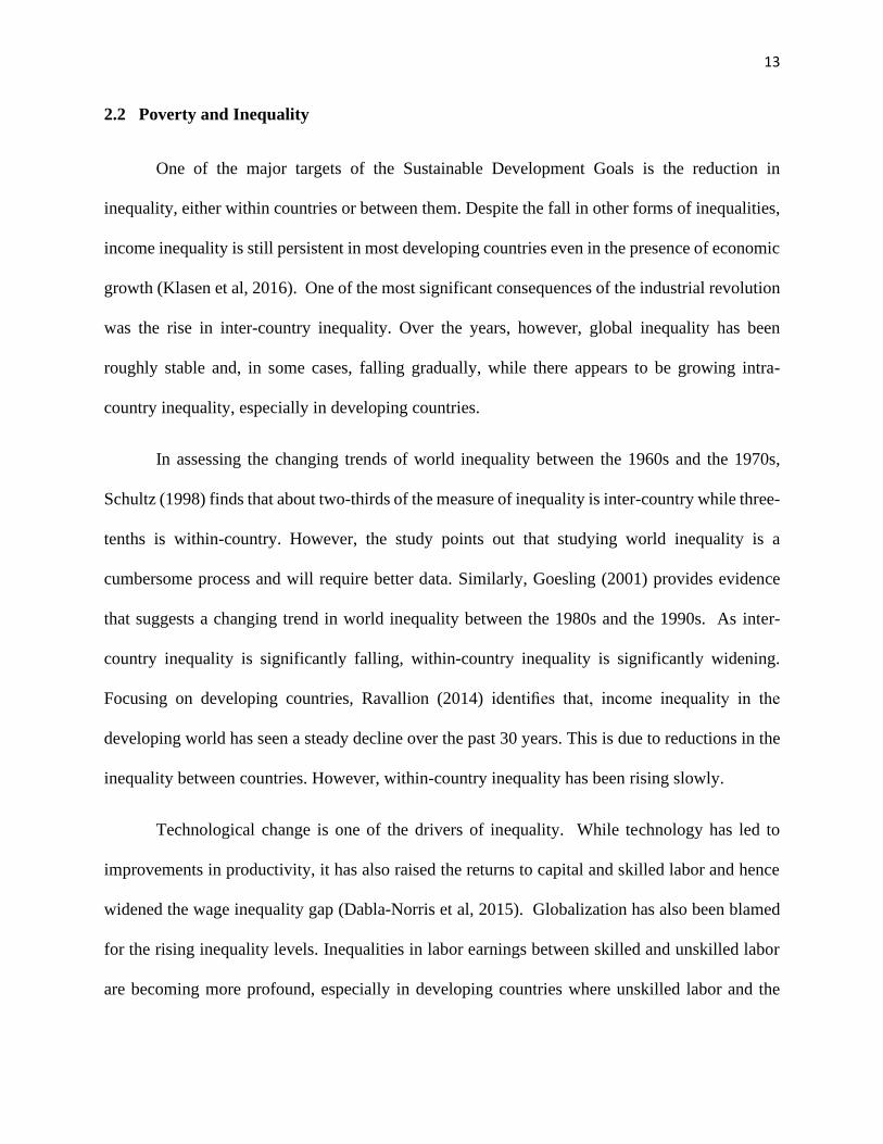
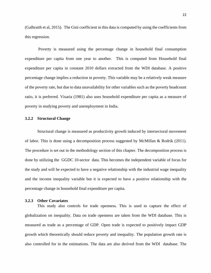
Figure 1 presents a scatter plot of agricultural employment shares and manufacturing

employment shares for Asian and SSA countries, while Figure 2 presents a scatter diagram of

agricultural employment shares and services employment shares for these same countries. Both

figures show a negative correlation between agricultural employment shares and the

manufacturing and service sector employment shares. As the agricultural employment shares fall,

employment shares in the manufacturing and service sectors rise. This reflects the apparent

structural change going on in these regions.

The pattern of the labor movement from the agricultural sector to the service sector shown

in Figure 2 is more apparent. This demonstrates that the service sector is growing very fast in

developing country economies. Authors argue that this movement into the service sector is not

growth-enhancing as the service sector is considered to be relatively less productive compared to

the manufacturing sector.

Figures 3 and 4 show the relationship between the agricultural employment share and

economy-wide productivity for SSA and Asian countries respectively. Both of these graphs show

a negative correlation between agricultural employment share and economy-wide productivity.

This is generally what is expected. Structural change, which leads to a reduction in agricultural

employment share and a rise in employment shares for other relatively more productive sectors, is

expected to coincide with an increase in economy-wide productivity. The negative pattern is more

clear for Asian countries compared to those from SSA. This could lend support to the argument

that structural change has been more growth-enhancing for Asia than for Sub-Saharan Africa.

32

Figure 1

Agricultural and Manufacturing Shares in Employment.

Figure 2

Agricultural and Services Shares in Employment

-.2

0.2

.4.6

.8

0 .1 .2 .3MANempshare

Ag share in employment Fitted values

Asia

-.5

0.5

10 .1 .2 .3

MANempshare

Ag share in employment Fitted values

SSA

Source: Authors generation with Stata

0.5

1

0 .2 .4 .6 .8service

AGRempshare Fitted values

Asia

0.5

1

0 .2 .4 .6 .8service

AGRempshare Fitted values

SSA

Source: Author's generation with Stata

33

Figure 3

Agricultural Employment Share and Productivity (SSA)

Figure 4

Agricultural Employment Share and Productivity (Asia)

ETHETHETHETHETHETHETHETHETHETHETHETHETHETHETHETHETHETHETHETHETHETHETHETHETHETHETHETHETHETHETHETHETHETH

ETH

ETHETHETHETHETHETHETH

ETHETHETHETHETH

GHAGHAGHAGHAGHAGHAGHAGHAGHAGHAGHAGHAGHAGHAGHAGHA

GHAGHAGHAGHAGHAGHAGHAGHAGHAGHAGHAGHAGHA

KENKENKENKENKENKENKENKENKEN

KENKENKEN

KEN

KEN

KEN

KEN

KEN

KEN

KEN

KENKEN

KEN

KENKENKENKENKENKENKENKEN

KEN

KENKENKENKENKENKENKEN

KENKEN

KEN

KEN

KEN

MWIMWIMWIMWIMWIMWIMWIMWIMWIMWIMWIMWIMWIMWIMWIMWIMWIMWIMWIMWIMWIMWIMWIMWIMWIMWIMWIMWIMWIMWIMWIMWIMWI

MWIMWIMWI

MWI

MWI

MWI

MWIMWIMWI

MUSMUSMUS

MUSMUSMUSMUSMUSMUSMUSMUSMUSMUSMUSMUSMUSMUS

MUSMUSMUSMUSMUSMUSMUSMUSMUSMUSMUSMUSMUSMUSMUSMUSMUSMUSMUSMUSMUSMUSMUSMUSMUS

NGANGANGANGANGANGANGA

NGANGANGA

NGA

NGANGA

NGANGANGANGANGANGA

NGANGA

NGA

NGA

NGA

NGA

NGANGA

NGA SENSENSENSENSENSENSENSENSENSENSEN

SENSENSENSENSEN

SENSENSENSEN

SEN

SEN

SENSENSENSENSENSEN

SENSENSENSENSENSENSENSENSEN

ZAFZAFZAFZAFZAFZAFZAFZAFZAFZAF

ZAFZAFZAF

ZAF

ZAFZAFZAFZAFZAFZAF

ZAF

ZAF

ZAF

ZAF

ZAFZAF

ZAFZAFZAFZAFZAFZAF

ZAF

ZAFZAFZAFZAFZAF

ZAF

ZAFZAF

ZAFZAFZAFZAFZAFZAFZAFZAF

TZATZATZATZATZATZATZATZATZATZATZATZATZATZATZATZATZATZA

TZATZATZATZATZATZATZATZATZATZATZA

TZATZATZATZATZATZATZATZATZA0

.2.4

.6.8

1

Ag s

ha

re in

em

plo

ym

en

t

0 2 4 6 8Log of Economy wide productivity

Ethiopia Ghana

Kenya Malawi

Mauritius Nigeria

Senegal South Africa

Tanzania

Source: Author's generation using data from GGDC

CHNCHNCHNCHNCHNCHNCHN

CHNCHNCHN

CHNCHNCHNCHNCHNCHNCHNCHN

INDINDINDINDINDINDINDINDINDINDINDINDINDINDINDINDINDINDINDINDINDINDINDINDINDINDINDINDINDINDINDINDINDINDINDINDINDINDINDINDINDINDINDINDINDINDINDIND

IDNIDNIDNIDNIDNIDNIDNIDN

IDNIDNIDNIDNIDNIDNIDNIDNIDNIDNIDNIDN

IDNIDNIDN

IDN

IDNIDNIDNIDNIDNIDNIDNIDNIDNIDNIDNIDNIDNIDNIDNIDN

IDNIDN

JPNJPNJPNJPNJPNJPNJPNJPNJPNJPNJPNJPNJPNJPNJPNJPNJPNJPNJPNJPNJPNJPNJPNJPNJPNJPNJPNJPNJPNJPNJPNJPNJPNJPNJPNJPNJPNJPNJPNJPNJPNJPNJPNJPNJPNJPNJPNJPN

MYSMYSMYSMYSMYS

MYSMYSMYSMYSMYSMYSMYSMYSMYS

MYSMYSMYSMYSMYSMYSMYSMYSMYSMYSMYSMYS

MYSMYSMYSMYSMYSMYSMYSMYSMYSMYSMYS

PHLPHLPHL

PHL

PHL

PHLPHL

PHLPHLPHL

PHL

PHLPHLPHL

PHLPHLPHLPHL

PHLPHLPHL

PHLPHL

PHLPHLPHL

PHLPHLPHL

PHL

PHLPHL

PHL

PHL

PHLPHLPHLPHLPHLPHLPHLPHL

THATHATHATHATHATHATHATHATHA

THATHATHATHATHATHA

THATHATHA

THATHA

THATHATHA

THATHA

0.2

.4.6

.8

Ag s

ha

re in

em

plo

ym

en

t

2 4 6 8 10Log of Economy wide productivity

China India

Indonesia Japan

Malaysia Philippines

Thailand

Source: Author's generation using data from GGDC

34

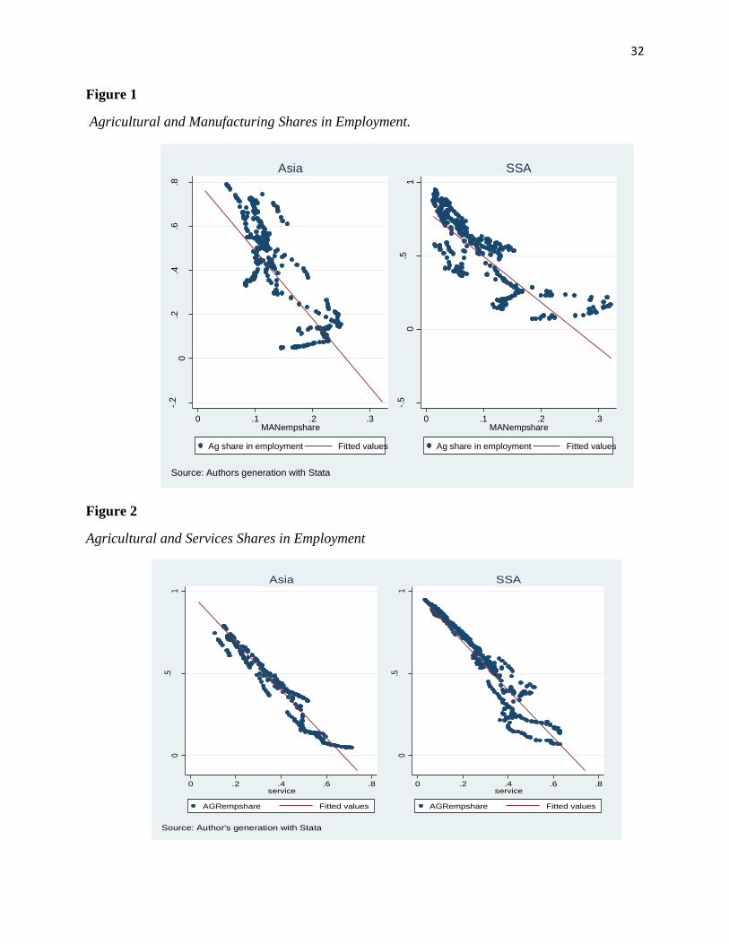
4.2 Agricultural Employment Shares and Inequality

Widening inequality in the face of structural change is of concern to economists and

policymakers. Figures 5 and 6 present scatter diagrams of agricultural employment shares and

industrial wage inequality and income inequality respectively. Both graphs show a positive

correlation between agricultural employment shares and inequality. Growth in agricultural

employment shares is associated with increasing inequality. This pattern is similar for all regions,

implying that structural change that results in the shrinking of the agricultural sector should also

reduce industrial wage inequality and income inequality.

Figure 5

Agricultural Employment Share and Sectoral Wage Inequality

0

.05

.1.1

5

0 .2 .4 .6 .8 1Ag share in employment

Sectoral wage inequality Fitted values

Asia

0

.05

.1.1

5.2


Sectoral wage inequality Fitted values

SSA


35

Figure 6

Income Inequality and Agricultural Employment Share

This is expected because of the wage gaps between the agricultural sector and other

relatively more productive sectors. The agricultural wage is relatively lower than that of other

sectors; hence, the movements of workers out of the agricultural sector is expected to increase

wages for all sectors. This is because the movement of labor affects the marginal productivity of

all sectors. Increased wages imply higher labor incomes, lowering income inequality.

Figures 7 and 8 present scatter diagrams of globalization measured by trade openness and

sectoral wage inequality and income inequality respectively. As theory predicts, globalization

reduces inequality. When trade between countries increases, countries benefit from expanded

markets and the inflow of technology. These benefits generate higher incomes which should

reduce poverty and inequality. Though the graphs show a negative relationship, the fitted lines are

not as steep. This could suggest that the effect of globalization on inequality is not that strong. This

30

35

40

45

50

55


UTIP GINI estimate Fitted values

Asia

35

40

45

50

55


UTIP GINI estimate Fitted values

SSA


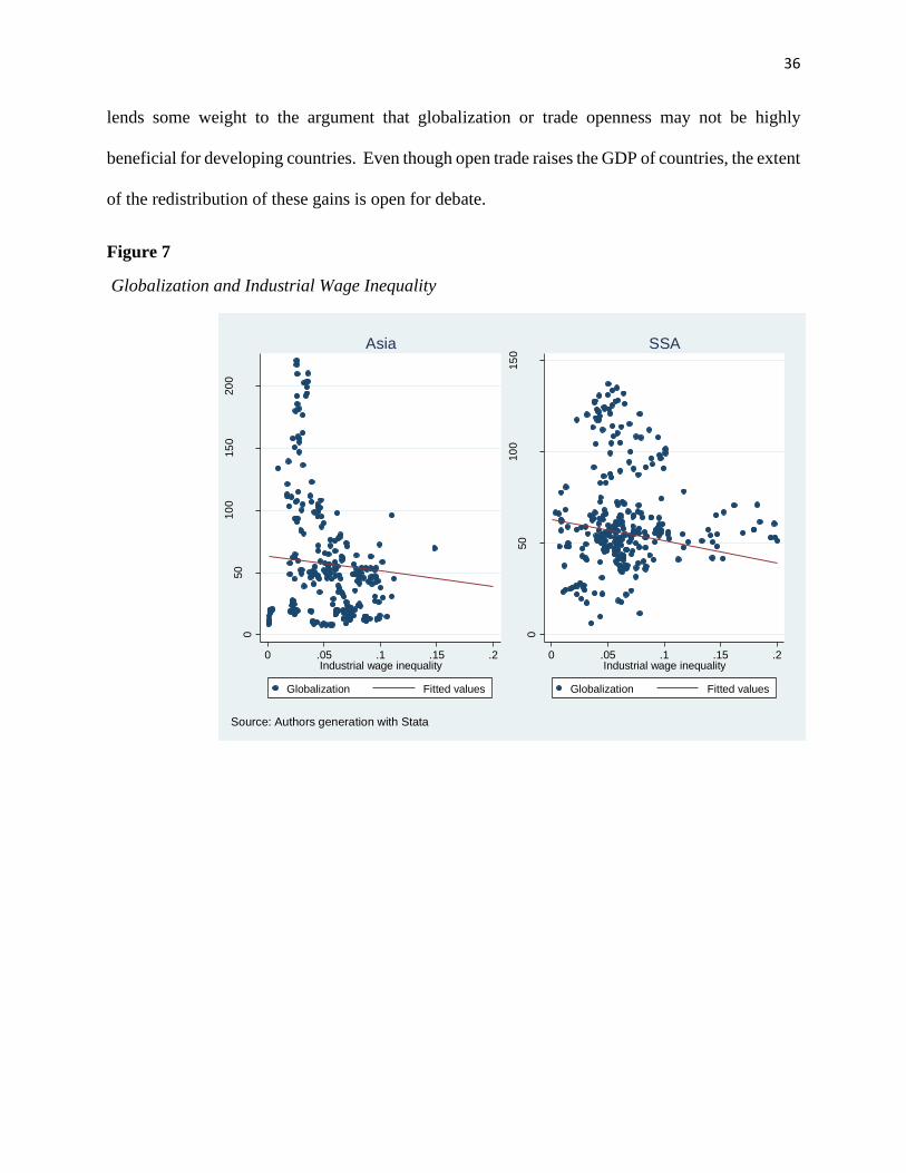
36

lends some weight to the argument that globalization or trade openness may not be highly

beneficial for developing countries. Even though open trade raises the GDP of countries, the extent

of the redistribution of these gains is open for debate.

Figure 7

Globalization and Industrial Wage Inequality

050

10

015

020

0

0 .05 .1 .15 .2Industrial wage inequality

Globalization Fitted values

Asia

050

10

015

0

0 .05 .1 .15 .2Industrial wage inequality


SSA


37

Figure 8

Globalization and Income Inequality

4.3 Descriptive Statistics

Table 1 below presents the descriptive statistics for the variables used in the model.

These are the values for all observations available in the data. The Theil index representing

industrial wage inequality ranges from 0.001 to 0.2. The mean value is 0.044 with a standard

deviation of 0.034. The Gini measure of income inequality averages about 42.9 for the period

under consideration. The standard deviation is about seven. The lowest Gini score in the

sample is 27.67 recorded by Sweden in 1975, while the largest Gini score is 56.65, recorded

by Malawi in 2009.

050

10

015

020

0

30 35 40 45 50 55UTIP GINI estimate


Asia

050

10

015

030 35 40 45 50 55

UTIP GINI estimate


SSA


38

The structural change share in productivity growth averages -0.002 with a standard

deviation of 0.158. The minimum value is -4.430 recorded by Bostwana in 1990, and the

maximum value is 2.242 recorded by Nigeria in 1995. This measure is what is obtained from

the decomposition of productivity growth as outlined in equation (4). It represents the part of

productivity growth that can be attributed to intersectoral labor movements. The difference

between the technological change effect and the structural change effect is computed as the

difference in the two terms in the right-hand side of equation 3. The mean is 0.003 with a

standard deviation of 0.296. The minimum value -2.570 is recorded by Indonesia in 1994 and

the maximum value of 6.043 is recorded again by Indonesia in 1991.

The average percentage change in household consumption per capita is 2.397 percent

with a standard deviation of 4.514 percent. The minimum value is -24.82 percent also recorded

by Nigeria in 1983 and the maximum value is 39.85 percent recorded by Kenya in 1971.

Inflation averaged about 17.8 percent for the sample with a standard deviation of 132.26

percent. The minimum value is -9.809 percent recorded by Ethiopia in 1986, and the maximum

value is 2947.7 percent recorded by Brazil in 1990. Brazil generally experienced hyperinflation

between the late 1980s to the early 1990s because of political turmoil triggered by the energy

crises of the 1970s.

Trade openness, measured as the sum of imports and exports taken as a percentage of

GDP averaged 58.57 percent with a standard deviation of 34.12 percent. The highest trade

openness value is about 220.4 percent of GDP recorded by Malaysia in 2000 and the lowest

value is 6.3 percent recorded by Ghana in 1982. Before 1982, Ghana was on an economic

downturn that saw drastic declines in living conditions. The recession was mainly due to bad

economic policies implemented by successive military governments that affected both imports

39

and exports. The result was the implementation of the Economic Recovery Program in 1982,

which among other goals sought to enhance Ghana’s trade with the rest of the world.

Table 1:

Summary Statistics

Mean St Dev Min Max Obs

Industrial wage gap

(Theil Index)

0.044 0.034 0.001 0.200 1023

Income inequality (Gini)

42.904 7.062 27.676 56.647 985

% change in household

consumption per capita

2.397 4.514 -24.821 39.849 788

Structural change share in

productivity

-0.002 0.158 -4.430 2.242 1043

Technological change share -

Structural change share

0.003 0.296 -2.570 6.043 1049

Inflation

17.814 132.262 -9.809 2947.733 1006

Trade openness

58.573 34.119 6.320 220.407 976

Agriculture employment share 36.5 28.9 1.7 94.8 1049

Human Capital Index

2.148 0.678 1.016 3.683 1049

Population growth

1.685 1.079 -0.073 6.008 1049

Unemployment

7.977 6.227 0.660 33.473 483

Income (log) 9.096 1.247 6.244 10.761 508

Agricultural employment share is computed as the ratio of the number of persons

employed in the agricultural sector to the total employment in all sectors defined in the GGDC

data. The mean value is 36.5 percent with a standard deviation of 28.9 percent. The minimum

value is 1.7 percent recorded by the United Kingdom in 2003 and the maximum value is 94.8

40

percent recorded by Ethiopia in 1965. Typically, developed countries like the United Kingdom

are expected to have a lower proportion of workers employed in the agricultural sector. This

is because these countries have already undergone the structural change process which

coincides with a decline in agricultural employment and a rise in employment in other sectors

of the economy. However, developing countries like Ethiopia will have higher agricultural

employment shares, especially during periods where these economies are transitioning towards

industrialization.

The human capital index averages 2.148 with a standard deviation of 0.678 over the

period under consideration. The minimum value of 1.02 is recorded by Ethiopia in 1965. It is

not surprising that human capital in Ethiopia was low at the same time that the agricultural

employment share was high. The maximum value of 3.68 was again recorded by the United

Kingdom in 2009. The population growth rate also averaged about 1.69 percent with a standard

deviation of 1.079 percent. The minimum population growth rate is -0.073 percent recorded

by Denmark in 1985. The highest population growth of about 6 percent was recorded by

Malawi in 1987. Unemployment rate averages about 8 percent with a standard deviation of

6.23 percent. The smallest unemployment rate of 0.66 percent was recorded by Thailand in

2011, and the highest unemployment rate of 33.47 percent was recorded by South Africa in

2002. The log of income also has a mean of about 9.1 with a standard deviation of 1.28. The

minimum value is 6.24 is recorded by Ethiopia in 1992 and the maximum value of 10.76 is

recorded by the Netherlands in 2008.

41

Chapter Five

Estimation Results

This chapter presents the results for the estimations carried out. Both parametric and non-

parametric techniques are employed. The first section presents the parametric estimates, while the

second section presents the nonparametric estimates. Three independent variables are employed:

the industrial wage inequality, the Gini coefficient measure of income inequality, and the

percentage change in household consumption per capita as a measure of poverty. Each set of

regressions is first done for the entire sample, and then separate regressions are run for the sub-

Saharan Africa and Asia subsamples.

5.1 Parametric Estimation Results.

In this section, standard panel data estimation techniques are employed. Pooled Ordinary

Least Squares techniques are first applied, and then the fixed and random-effects models are

performed. The results of all these models are presented for comparison. Because these models

have different assumptions about the country fixed-effects, the results may be different across

them. This allows for comparing relations under different assumptions. Two major diagnostic tests

will be carried out to determine which model is better. The first test will be the Hausman test,

which determines whether the fixed or the random-effects models are better. In a case where the

random-effects model is selected as best, the Breusch Pagan Lagrange Multiplier (BP-LM) test

will be conducted to determine whether the random-effects or the pooled OLS results are

appropriate. Two stars are placed on the column name for the results that are shown to be preferred.

The results are first presented for the full sample, and then the results for the SSA and Asia

subsamples are shown. To ensure robustness, all regressions are estimated with robust standard

errors.

42

5.1.1 Industrial Wage Inequality

This section presents the results for estimations that use industrial wage inequality as the

dependent variable. Table 2 provides the results for the full sample.

Table 2

Structural Change and Industrial Wage Inequality- Full Sample

(1) (2) (3)

VARIABLES Pooled OLS FE** RE

Structural change share -0.0006 -0.0120*** -0.0115***

(0.0125) (0.0018) (0.0016)

L.structural change share 0.0017 -0.0015*** 0.0002

(0.0047) (0.0005) (0.0003)

Inflation 0.0000*** -0.0000 -0.0000

(0.0000) (0.0000) (0.0000) Technical change-structural change 0.0020 -0.0033*** -0.0041***

(0.0062) (0.0010) (0.0008) Log_income -0.0432 0.0711 0.0767

(0.0330) (0.0603) (0.0724) Log_income*Log_income 0.0006 -0.0045 -0.0060

(0.0017) (0.0036) (0.0041)

Trade openness -0.0001*** 0.0001 0.00004

(0.0000) (0.0001) (0.0001) Agriculture employment share -0.0141 -0.0844** -0.0215

(0.0250) (0.0304) (0.0318) Human Capital Index 0.0109** 0.0285** 0.0489***

(0.0054) (0.0131) (0.0133) Unemployment 0.0006*** 0.0016*** 0.0010**

(0.0002) (0.0006) (0.0004) Population growth -0.0032 0.0101*** 0.0086***

(0.0023) (0.0026) (0.0029)

Constant 0.3829** -0.2987 -0.2719

(0.1668) (0.2616) (0.3316)

Observations 416 416 416

R-squared 0.5785 0.1754

Number of Countries 27 27

Robust standard errors in parentheses

*** p<0.01, ** p<0.05, * p<0.1

FE** Fixed Effects is preferred

43

Based on the Hausman test, the preferred model is the fixed-effects model. The results

show that structural change is found to reduce industrial wage inequality as expected. This

relationship is the same across all models. The coefficients for both the fixed-effects and random-

effects models are statistically significant at one percent level, while that of the pooled OLS is not

significant. From the fixed effects results, a one-point increase in the structural change share in

productivity results in about 0.012 points reduction in the industrial wage inequality index, other

variables held constant. The lagged value of structural change is also negative and statistically

significant for the fixed effects model, implying that a one-point increase in the lagged value of

structural change significantly reduces the average industrial wage inequality by about 0.002

points, other variables held constant. This implies that the effect of structural change on the

industrial wage inequality is more dynamic than static. This makes sense because the effect of

structural change may take time to reflect.

Inflation has no significant effect on industrial wage inequality. The gap between technical

change and structural change is found to reduce industrial wage inequality. This is statistically

significant at one percent. The coefficient implies that a unit increase in the gap between technical

change and structural change reduces industrial wage inequality by 0.0033 points, other variables

held constant. The log of income and its squared term are both statistically insignificant. Trade

openness also has no significant effect on industrial wage inequality.

Agricultural employment share is found to significantly reduce industrial wage inequality.

A one-point increase in the agricultural share of employment reduces industrial wage inequality

by about 0.084 points, other variables held constant. An increase in the relative agricultural

employment share implies that productivity in this sector is rising; hence, as labor move into the

sector, it is expected to reduce the industrial wage inequality. Human capital is found to

44

significantly worsen industrial wage inequality. A unit increase in the human capital index results

in about a 0.029 point increase in industrial wage inequality, other variables held constant. As

expected, unemployment is found to increase industrial wage inequality. A percentage point

increase in the unemployment rate increases industrial wage inequality by about 0.0017 points on

average. The population growth rate is also found to significantly increase industrial wage

inequality. A unit increase in the population growth rate increases industrial wage inequality by

about 0.01 points on average.

Table 3 presents the results for the sub-Saharan Africa sub-sample of countries. Again, the

Hausman test goes in favor of the fixed-effects model. Structural change is again found to reduce

industrial wage inequality. The coefficient is significant at a ten-percent level of significance.

Other variables held constant, a one-point increase in structural change share in productivity results

in about a 0.004 point reduction in the industrial wage inequality. The lagged value of structural

change share has a negative sign as well but it is statistically insignificant.

As expected, inflation also increases industrial wage inequality. A percentage point

increase in inflation increases industrial wage inequality by an average of 0.0004 points, other

variables held constant. The gap between technical change and structural change is found to

significantly reduce industrial wage inequality for sub-Saharan African countries. Other variables

held constant a one-point increase in the gap leads to about a 0.34 point average reduction in the

industrial wage inequality.

45

Table 3

Structural Change and Industrial Wage Inequality-SSA Subsample

(1) (2) (3)


Structural change share 0.0134 -0.0043* 0.0134

(0.0085) (0.0023) (0.0141) L.structural change share 0.0048 -0.0001 0.0048*

(0.0035) (0.0011) (0.0025)

Inflation 0.0002 0.0004* 0.0002

(0.0003) (0.0002) (0.0003) Technical change-structural change -0.1958 -0.3395*** -0.1958

(0.2116) (0.0549) (0.3152) Log_Income -0.5305*** 0.2685** -0.5305***

(0.1142) (0.1013) (0.1266) Log_income*Log_income 0.0298*** -0.0159** 0.0298***

(0.0070) (0.0058) (0.0076) Trade openness 0.0001 -0.0002 0.0001

(0.0002) (0.0001) (0.0002) Agriculture employment share -0.0497 -0.0732** -0.0497

(0.0393) (0.0266) (0.0349) Human Capital Index 0.0370*** 0.0512** 0.0370***

(0.0105) (0.0201) (0.0142) Unemployment 0.0008 0.0018 0.0008

(0.0006) (0.0013) (0.0007) Population growth 0.0186** 0.0099*** 0.0186***

(0.0081) (0.0015) (0.0062)

Constant 2.2841*** -1.1393** 2.2841***

(0.4725) (0.4477) (0.5301)


R-squared 0.6411 0.2624



*** p<0.01, ** p<0.05, * p<0.1


The coefficient on income is positive while the squared term is negative as expected. The

average marginal effect for income is about 0.01, implying that a percentage-point increase in

income generally leads to a 0.01 point increase in industrial wage inequality. It is not surprising

46

that the overall effect is positive for sub-Saharan Africa because most of these countries are still

at developing stages, we expect that growth in GDP will widen industrial wage inequality.

Trade openness has no significant effect on industrial wage inequality in sub-Saharan

Africa. Agricultural employment share is found to significantly reduce industrial wage inequality.

On average, a one-point increase in agricultural shares in employment results in about 0.073 point

reduction in industrial wage inequality, other variables held constant. Human capital is also found

to widen industrial wage inequality for sub-Saharan Africa. The coefficient implies that a unit

increase in the human capital index results in about a 0.051 point increase in industrial wage

inequality on average. This strong effect implies that the quality of human capital contributes

significantly to the growing industrial wage gaps in the sub-region. Unemployment has the

expected positive sign, but it is not statistically significant. The population growth rate also has

the expected positive sign and is statistically significant. A percentage point increase in the

population growth rate results in a 0.01 point increase in industrial wage inequality, other variables

held constant.

Table 4 presents the results for the Asian subsample of countries. Again, the Hausman test

favors the fixed-effects model. Structural change share in productivity is found to have a negative

relationship with industrial wage inequality as expected. However, only the lag of structural

change share is statistically significant. A one-point increase in the previous year’s structural

change share in productivity reduces industrial wage inequality by approximately 0.04 points on

average, other variables held constant.

As expected, inflation worsens industrial wage inequality. The coefficient is significant at

the five percent level of significance. A percentage point increase in the inflation rate results in

about 0.0008 point increase in industrial wage inequality, other variables held constant.

47

Table 4

Structural Change and Industrial Wage Inequality-Asia Subsample

(1) (2) (3)


Structural change share 0.0073 -0.0167 0.0073

(0.0243) (0.0368) (0.0310) L.structural change share -0.0122 -0.0369*** -0.0122

(0.0131) (0.0051) (0.0153)

Inflation 0.0008*** 0.0008*** 0.0008**

(0.0002) (0.0002) (0.0004) Technical change-structural change 0.0006 0.0017** 0.0006

(0.0019) (0.0006) (0.0005) Log_Income -0.2484*** 0.1067 -0.2484**

(0.0646) (0.1368) (0.1240) Log_income*Log_income 0.0145*** -0.0070 0.0145**

(0.0036) (0.0095) (0.0073)

Trade openness -0.0001** 0.0000 -0.0001

(0.0001) (0.0001) (0.0001) Agriculture employment share 0.1390** 0.0083 0.1390

(0.0579) (0.1507) (0.1117) Human Capital Index 0.0198 0.0669* 0.0198

(0.0133) (0.0308) (0.0245) Unemployment 0.0059*** 0.0042 0.0059**

(0.0022) (0.0041) (0.0028) Population growth 0.0134* 0.0155 0.0134

(0.0075) (0.0160) (0.0185)

Constant 0.9779*** -0.5409 0.9779**

(0.2982) (0.5713) (0.4699)


R-squared 0.5340 0.2590



*** p<0.01, ** p<0.05, * p<0.1


For Asia, the gap between technical change and structural change worsens industrial wage

inequality. A one-point increase in the gap results in a 0.002 point increase in industrial wage

inequality, other variables held constant. This is also significant at five percent level of

significance. Income and its squared term again have the expected signs even though they are

48

insignificant. Trade openness and agricultural employment share have a positive but insignificant

effect on industrial wage inequality. Human capital is also found to exacerbate industrial wage

inequality. A one-point increase in the human capital index results in a 0.069 point increase in

industrial wage inequality. Unemployment and population growth are found to worsen industrial

wage inequality, even though their coefficients are not statistically significant.

5.1.2 Income Inequality

This section presents the results for the estimations with income inequality as the dependent

variable. Income inequality is measured using the University of Texas Inequality Project (UTIP)

Gini estimates of income inequality. Their Gini estimates have more observations than the Gini

coefficient estimates of the World Bank.

Table 5 presents the results for the full sample. The fixed-effects model is again the

preferred model under this estimation. The results show that both structural change and the lagged

value of structural change lead to a reduction in income inequality. A one-point increase in current

structural change share results in about a 0.84 point reduction in income inequality, other variables

held constant. Previous increases in structural change share also reduce current income inequality.

However, the impact relatively smaller. A one-point increase in the previous year’s value of

structural change results in about 0.19 point reduction in income inequality, other variables held

constant. Both coefficients are statistically significant.

As expected, inflation is found to worsen income inequality even though the coefficient is

relatively small. The gap between technological change and structural change is found to be

income inequality-reducing, even though it is not significant.

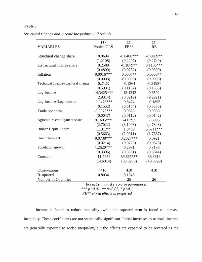
49

Table 5

Structural Change and Income Inequality: Full Sample

(1) (2) (3)


Structural change share 0.0694 -0.8406*** -0.6069**

(1.2108) (0.2297) (0.2749)

L.structural change share 0.2589 -0.1879** 0.1103***

(0.4809) (0.0762) (0.0390)

Inflation 0.0016*** 0.0007** 0.0006**

(0.0003) (0.0003) (0.0003) Technical change-structural change 0.2123 -0.1364 -0.2198*

(0.5931) (0.1137) (0.1335) Log_income 14.3425*** -13.4242 0.6502

(2.9314) (8.3219) (9.2921) Log_income*Log_income -0.9478*** 0.8474 -0.1895

(0.1552) (0.5154) (0.5355)

Trade openness -0.0378*** 0.0026 0.0058

(0.0047) (0.0112) (0.0142) Agriculture employment share 9.1695*** -4.0393 7.8093

(2.7022) (3.1903) (4.7843) Human Capital Index 1.1312** 1.3409 5.6211***

(0.5663) (2.0011) (1.7887) Unemployment 0.0738*** 0.2027*** 0.0921

(0.0214) (0.0720) (0.0675) Population growth 1.2520*** 0.2931 0.3136

(0.3306) (0.3391) (0.3844)

Constant -11.7859 89.6655** 36.8618

(14.6014) (33.0250) (40.3829)


R-squared 0.8034 0.1646



*** p<0.01, ** p<0.05, * p<0.1

FE** Fixed effects is preferred

Income is found to reduce inequality, while the squared term is found to increase

inequality. These coefficients are not statistically significant. Initial increases in national income

are generally expected to widen inequality, but the effects are expected to be reversed as the

50

economy matures. Trade openness, human capital, and population growth are both found to

increase income inequality, but they are not statistically significant. Agricultural employment

share is found to reduce income inequality, but it is also statistically insignificant. As expected,

unemployment widens income inequality. Income inequality increases by approximately 0.29

points in response to a one-percentage-point increase in the unemployment rate.

Table 6 presents the results for the sub-Saharan Africa subsample of countries. Again, the

fixed effects model is the most preferred. The results show that structural change has no significant

effect on income inequality in sub-Saharan Africa. Though the signs show that structural change

is growth reducing, they are not statistically significant. Inflation worsens inequality and is

statistically significant. A one-percentage-point increase in inflation will result in about a 0.028

point increase in income inequality, other variables held constant. The gap between technical

change and structural change is found to significantly reduce income inequality. A one-point

increase in the gap results in about a 28.6 point reduction in income inequality, other variables

held constant. Income and the squared of income have the expected signs but are again not

statistically significant. Trade openness is found to reduce income inequality as expected, but the

coefficient is not statistically significant.

The agricultural employment share is found to significantly reduce income inequality. A

one-point increase in the agricultural employment share results in about a 7.28 point reduction in

income inequality. This finding is not surprising given the fact that agriculture is still a hugely

important part of the economies of sub-Saharan African countries. Human capital and

unemployment are both found to worsen income inequality but are not statistically significant.

Population growth however significantly widens income inequality. A percentage-point increase

51

in population growth rate results in about a 0.48-point increase in income inequality, other

variables held constant.

Table 6

Structural Change and Income Inequality: SSA Subsample

(1) (2) (3)


Structural change share 1.2594* -0.3331 1.2594

(0.7510) (0.2150) (1.3872) L.structural change share -0.0504 -0.1324 -0.0504

(0.4063) (0.2116) (0.2565)

Inflation 0.0198 0.0274* 0.0198

(0.0175) (0.0146) (0.0196) Technical change-structural change -2.4901 -28.6445*** -2.4901

(17.8670) (5.5819) (28.1826) Log_Income -23.8215*** -11.8878 -23.8215***

(6.7370) (9.8056) (9.0146) Log_income*Log_income 1.3679*** 0.9012 1.3679**

(0.4226) (0.5944) (0.6028)

Trade openness -0.0493*** -0.0135 -0.0493*

(0.0125) (0.0084) (0.0286) Agriculture employment share 11.7997*** -7.2862** 11.7997*

(3.2262) (2.4636) (6.0206) Human Capital Index 4.1284*** 1.6734 4.1284***

(0.9254) (1.8055) (1.4293) Unemployment 0.1215*** 0.1828 0.1215**

(0.0379) (0.1339) (0.0610) Population growth 1.5172*** 0.4863** 1.5172***

(0.4751) (0.1703) (0.5114)

Constant 135.3364*** 82.2801* 135.3364***

(27.5101) (43.1389) (34.3769)


R-squared 0.8712 0.3319



*** p<0.01, ** p<0.05, * p<0.1

FE** Fixed-effects is preferred

Table 7 presents the results for the Asia subsample of countries. The fixed-effects model

is again the most preferred. The results show that, though current structural change values have

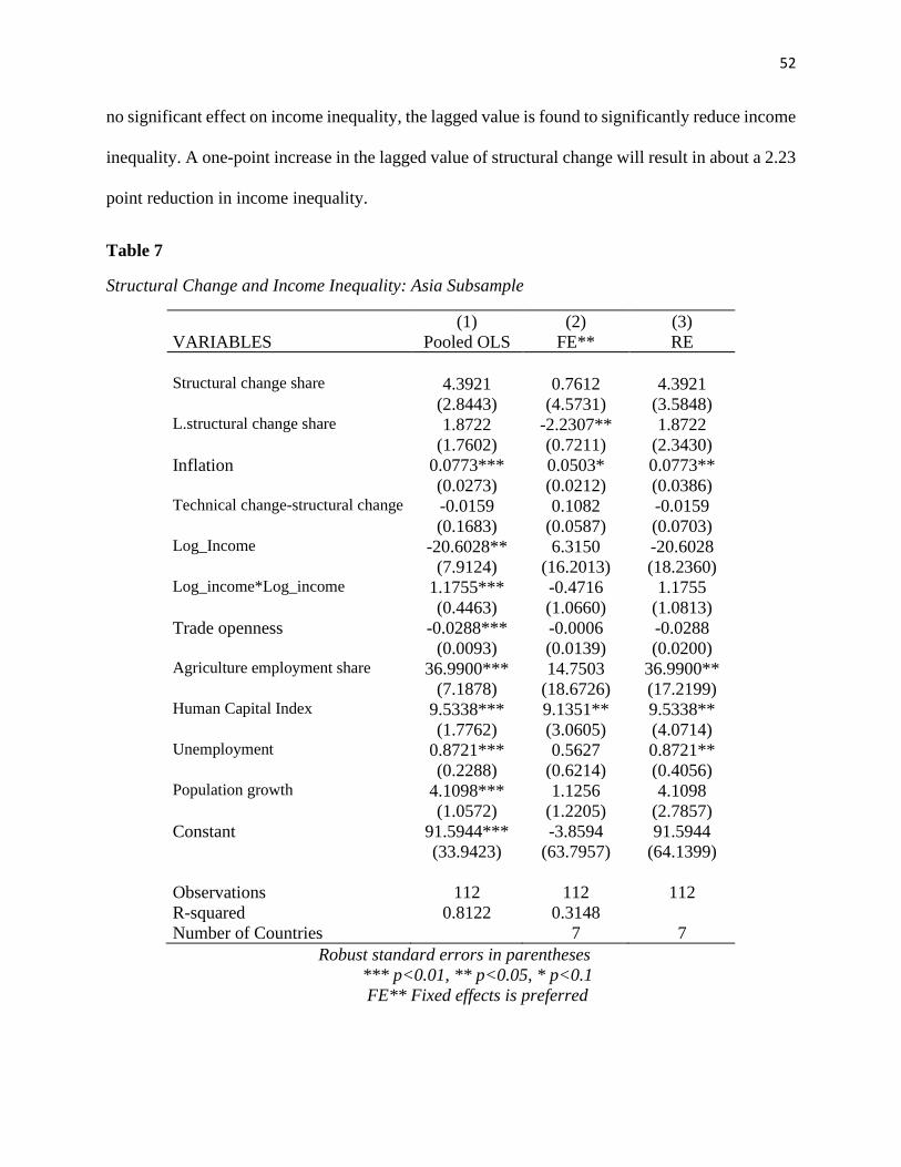
52

no significant effect on income inequality, the lagged value is found to significantly reduce income

inequality. A one-point increase in the lagged value of structural change will result in about a 2.23

point reduction in income inequality.

Table 7

Structural Change and Income Inequality: Asia Subsample

(1) (2) (3)


Structural change share 4.3921 0.7612 4.3921

(2.8443) (4.5731) (3.5848) L.structural change share 1.8722 -2.2307** 1.8722

(1.7602) (0.7211) (2.3430)

Inflation 0.0773*** 0.0503* 0.0773**

(0.0273) (0.0212) (0.0386) Technical change-structural change -0.0159 0.1082 -0.0159

(0.1683) (0.0587) (0.0703) Log_Income -20.6028** 6.3150 -20.6028

(7.9124) (16.2013) (18.2360) Log_income*Log_income 1.1755*** -0.4716 1.1755

(0.4463) (1.0660) (1.0813)

Trade openness -0.0288*** -0.0006 -0.0288

(0.0093) (0.0139) (0.0200) Agriculture employment share 36.9900*** 14.7503 36.9900**

(7.1878) (18.6726) (17.2199) Human Capital Index 9.5338*** 9.1351** 9.5338**

(1.7762) (3.0605) (4.0714) Unemployment 0.8721*** 0.5627 0.8721**

(0.2288) (0.6214) (0.4056) Population growth 4.1098*** 1.1256 4.1098

(1.0572) (1.2205) (2.7857)

Constant 91.5944*** -3.8594 91.5944

(33.9423) (63.7957) (64.1399)


R-squared 0.8122 0.3148



*** p<0.01, ** p<0.05, * p<0.1


53

Inflation also has a significant effect on income inequality, other variables held constant.

A percentage-point increase in the inflation rate raises income inequality by about 0.05 points. The

gap between technological change and structural change is found to increase income inequality

though its effect is not statistically significant.

Again, income and its squared term have the expected signs but are not statistically

significant. Trade openness also has a negative but statistically insignificant effect on income

inequality. The agricultural employment share is found to increase income inequality though its

effect is not statistically significant. Human capital is also found to significantly increase income

inequality. A one-point increase in the human capital index results in about a 9.14 point increase

in income inequality. Unemployment and population growth do not have any significant effect on

income inequality.

5.1.3 Poverty

This section presents the results for the impact of structural change on poverty. Poverty

here is measured using the percentage change in household consumption per capita from one year

to another. A positive value of this percentage change implies a reduction in poverty. Table 8

presents the results for the full sample. The Hausman test again goes in favor of the fixed-effects

model. Structural change is found to increase household consumption per capita. The lagged value

of structural change also increases the change in household per capita consumption. The

coefficients imply that a one-point increase in current structural change share increases the change

in per capita household consumption by about 4.92 percentage points on average. A change in the

lagged value of structural change share also increases the change in household consumption per

capita by approximately 0.5 percentage points, other variables held constant.

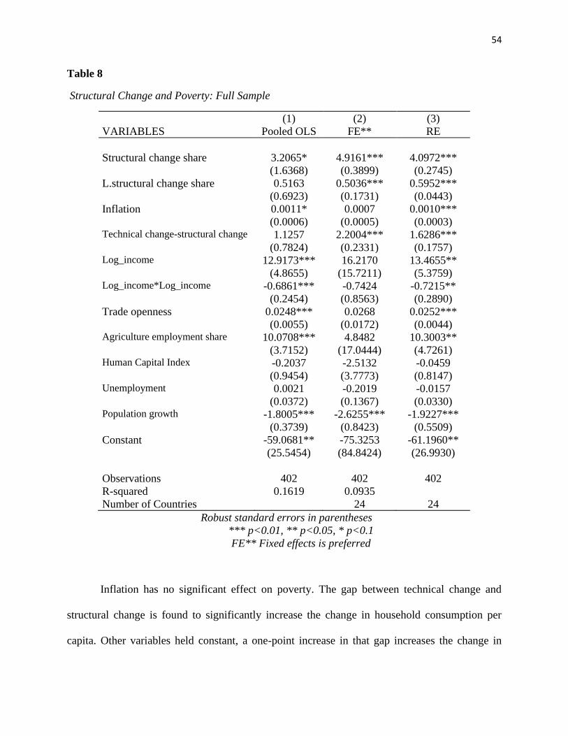
54

Table 8

Structural Change and Poverty: Full Sample

(1) (2) (3)


Structural change share 3.2065* 4.9161*** 4.0972***

(1.6368) (0.3899) (0.2745)

L.structural change share 0.5163 0.5036*** 0.5952***

(0.6923) (0.1731) (0.0443)

Inflation 0.0011* 0.0007 0.0010***

(0.0006) (0.0005) (0.0003) Technical change-structural change 1.1257 2.2004*** 1.6286***

(0.7824) (0.2331) (0.1757) Log_income 12.9173*** 16.2170 13.4655**

(4.8655) (15.7211) (5.3759) Log_income*Log_income -0.6861*** -0.7424 -0.7215**

(0.2454) (0.8563) (0.2890)

Trade openness 0.0248*** 0.0268 0.0252***

(0.0055) (0.0172) (0.0044) Agriculture employment share 10.0708*** 4.8482 10.3003**

(3.7152) (17.0444) (4.7261) Human Capital Index -0.2037 -2.5132 -0.0459

(0.9454) (3.7773) (0.8147) Unemployment 0.0021 -0.2019 -0.0157

(0.0372) (0.1367) (0.0330) Population growth -1.8005*** -2.6255*** -1.9227***

(0.3739) (0.8423) (0.5509)

Constant -59.0681** -75.3253 -61.1960**

(25.5454) (84.8424) (26.9930)


R-squared 0.1619 0.0935



*** p<0.01, ** p<0.05, * p<0.1


Inflation has no significant effect on poverty. The gap between technical change and

structural change is found to significantly increase the change in household consumption per

capita. Other variables held constant, a one-point increase in that gap increases the change in

55

household consumption per capita by about 2.2 percentage points, other variables held constant.

This implies that the widening of this gap reduces poverty. Therefore, as technologically driven

productivity rises, it is expected to reduce poverty, which is not surprising.

Income is found to increase household consumption per capita, while its squared term is

has a negative effect. However, these coefficients are not statistically significant. As expected,

trade openness is found to increase household consumption expenditure but is not statistically

significant. Agricultural employment share, human capital, and unemployment also have no

significant effect on poverty. Population growth significantly increases poverty as expected. A

percentage-point increase in the population growth rate reduces the change in household

consumption per capita by about 2.6 percentage points on average, other variables held constant.

Table 9 presents the results for the SSA subsample of countries. Again, the Hausman test

goes in favor of the fixed-effects model. The results show that structural change significantly

increases the change in household consumption per capita. On average, a one-point increase in the

structural change share in productivity results in a 5.2 percentage points increase in the change in

household consumption per capita, other variables held constant. The lagged value of structural

change share has no significant effect on poverty. As expected, inflation is found to increase

poverty in sub-Saharan Africa. A percentage-point increase in the inflation rate decreases the

change in household consumption per capita by about 0.44 percentage points, holding constant the

other variables. As expected, the log of income is found to reduce per capita consumption while

its square term has a positive effect, but these coefficients are statistically insignificant. The gap

between technological change and structural change shares is also found to widen poverty as

expected, but its effect is not statistically significant. Trade openness is found to significantly

reduce poverty by increasing the change in household consumption per capita. On average, a

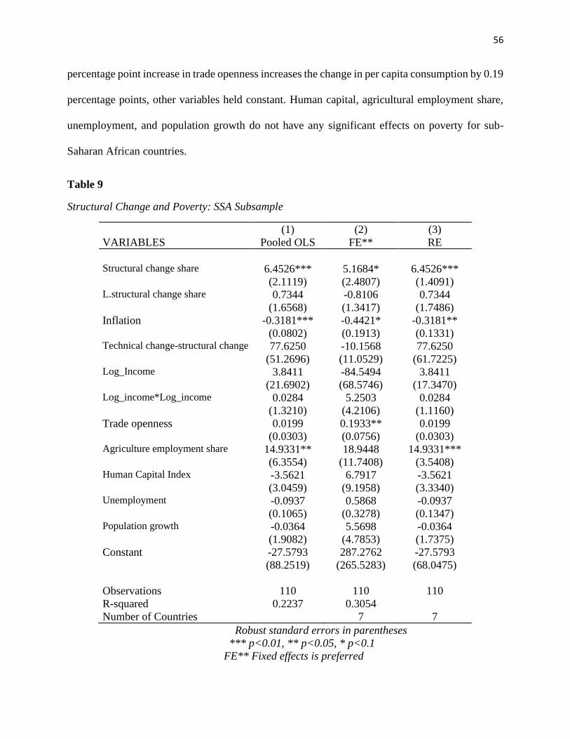
56

percentage point increase in trade openness increases the change in per capita consumption by 0.19

percentage points, other variables held constant. Human capital, agricultural employment share,

unemployment, and population growth do not have any significant effects on poverty for sub-

Saharan African countries.

Table 9

Structural Change and Poverty: SSA Subsample

(1) (2) (3)


Structural change share 6.4526*** 5.1684* 6.4526***

(2.1119) (2.4807) (1.4091) L.structural change share 0.7344 -0.8106 0.7344

(1.6568) (1.3417) (1.7486)

Inflation -0.3181*** -0.4421* -0.3181**

(0.0802) (0.1913) (0.1331) Technical change-structural change 77.6250 -10.1568 77.6250

(51.2696) (11.0529) (61.7225) Log_Income 3.8411 -84.5494 3.8411

(21.6902) (68.5746) (17.3470) Log_income*Log_income 0.0284 5.2503 0.0284

(1.3210) (4.2106) (1.1160)

Trade openness 0.0199 0.1933** 0.0199

(0.0303) (0.0756) (0.0303) Agriculture employment share 14.9331** 18.9448 14.9331***

(6.3554) (11.7408) (3.5408) Human Capital Index -3.5621 6.7917 -3.5621

(3.0459) (9.1958) (3.3340) Unemployment -0.0937 0.5868 -0.0937

(0.1065) (0.3278) (0.1347) Population growth -0.0364 5.5698 -0.0364

(1.9082) (4.7853) (1.7375)

Constant -27.5793 287.2762 -27.5793

(88.2519) (265.5283) (68.0475)


R-squared 0.2237 0.3054



*** p<0.01, ** p<0.05, * p<0.1


57

Table 10

Structural Change and Poverty: Asia Subsample

(1) (2) (3)


Structural change share 1.2687 2.0284 1.2687

(2.5614) (1.0496) (1.4800) L.structural change share 0.2356 0.7405 0.2356

(3.2801) (2.3652) (3.2481)

Inflation -0.2192*** -0.2302*** -0.2192***

(0.0374) (0.0282) (0.0236) Technical change-structural change 0.0631 0.0279 0.0631

(0.1993) (0.1252) (0.0628) Log_Income 33.0115*** -24.4975 33.0115***

(7.3244) (27.0501) (7.3819) Log_income*Log_income -1.9366*** 2.1085 -1.9366***

(0.4161) (1.9691) (0.4403)

Trade openness 0.0192 0.0205 0.0192*

(0.0118) (0.0184) (0.0115) Agriculture employment share -18.0707** 0.2335 -18.0707*

(7.2674) (17.3636) (9.8940) Human Capital Index -8.7460*** -26.5771 -8.7460***

(1.8277) (14.7078) (2.3370) Unemployment -0.4050*** 0.2576 -0.4050**

(0.1434) (0.5087) (0.1581) Population growth -4.5177*** -7.2676 -4.5177***

(0.7769) (4.4285) (1.1912)

Constant -99.9142*** 125.5226 -99.9142***

(30.6055) (117.9702) (24.0496)


R-squared 0.4745 0.3151



*** p<0.01, ** p<0.05, * p<0.1


Table 10 presents the regression results for the Asia subsample of countries. The Hausman

test again goes in favor of the fixed-effects model. Structural change is found to have no significant

effect on poverty in Asia. Only inflation has a significant effect on poverty for Asia. Inflation

58

increases poverty by reducing the change in per capita household consumption. A percentage point

increase in the inflation rate on average results in a 0.23 percentage point reduction in household

consumption per capita, other variables held constant. The log of income and its squared term have

the expected signs but are not statistically significant. Trade openness, human capital,

unemployment, unemployment, and population growth also have no significant effects on poverty

in Asia.

5.2 Non-Parametric Estimations

This section presents the results for the non-parametric estimation results. Following the

recommendation of Li et al. (2011), the local dummy variable technique is applied. As mentioned

earlier two main procedures are suggested for estimation of the time-varying coefficients. These

are the average local linear estimator and the pooled local dummy variable technique. They argue

that the pooled local dummy variable technique is more appropriate because the estimated trend

and coefficient functions have better convergence rates.

This procedure computes estimates for each period, rather than produce point estimates as

parametric techniques do. This allows for a plot of the coefficients across time and therefore, we

can generate graphs of the time-varying coefficients for each of the independent variables and a

trend function as well. This way, we can easily see how the coefficients change over time and can

then can make a judgment on the nature of the relationships between the dependent and

independent variables.

Once again, the results are estimated for all three dependent variables. For each dependent

variable, graphs are presented for the full sample and then for the SSA and Asia subsamples. The

59

estimation is done for only the period 1990 to 2012 because the procedure requires a balanced

panel and can only utilizes periods where the dataset is complete for all observations without gaps.

5.2.1 Industrial Wage Inequality

The set of graphs below (Figures 9-11) present the results for the non-parametric

estimations for industrial wage inequality. Figure 9 presents the results for the full sample of

countries.

Figure 9

Non-Linear Time-Varying Coefficients- Industrial Wage Inequality- Full Sample

Some of the coefficients of structural change are negative while others are positive. This

implies that structural change exacerbates income inequality for some years and reduces wage

inequality for other years. The coefficients of the lagged structural change variable are also

negative for some years and positive for others. These different signs of the coefficients suggest

0

10

020

030

0

Coe

ffic

ient-

Ve

cto

r 1,

orig

inal

1990 1995 2000 2005 2010coefsa_tvprime

Trend

-1-.

50

Coe

ffic

ient-

Ve

cto

r 2,

orig

inal

1990 1995 2000 2005 2010coefsa_tvprime

Structural change share-.

05

0

.05

.1

Coe

ffic

ient-

Ve

cto

r 3,

orig

inal

1990 1995 2000 2005 2010coefsa_tvprime

Lag of Structural change

-.03

-.02

-.01

0

.01

Coe

ffic

ient-

Ve

cto

r 4,

orig

inal

1990 1995 2000 2005 2010coefsa_tvprime

Inflation

-.5

-.4

-.3

-.2

-.1

0

Coe

ffic

ient-

Ve

cto

r 5,

orig

inal

1990 1995 2000 2005 2010coefsa_tvprime

T_change - S_change

010

20

30

Coe

ffic

ient-

Ve

cto

r 6,

orig

inal

1990 1995 2000 2005 2010coefsa_tvprime

Log_lnincome

-30

0-2

00

-10

0

0

Coe

ffic

ient-

Ve

cto

r 7,

orig

inal

1990 1995 2000 2005 2010coefsa_tvprime

Log_lnincome squared-.

01-.

00

5

0

.00

5.0

1.0

15

Coe

ffic

ient-

Ve

cto

r 8,

orig

inal

1990 1995 2000 2005 2010coefsa_tvprime

Trade Openness

02

46

8

Coe

ffic

ient-

Ve

cto

r 9,

orig

inal

1990 1995 2000 2005 2010coefsa_tvprime

Agric Emp share

-15

-10

-50

5

Coe

ffic

ient-

Ve

cto

r 10

, ori

gin

al

1990 1995 2000 2005 2010coefsa_tvprime

Human Capital Index

-.2

0.2

.4.6

Coe

ffic

ient-

Ve

cto

r 11

, ori

gin

al

1990 1995 2000 2005 2010coefsa_tvprime

Unemployment Rate

-20

24

68

Coe

ffic

ient-

Ve

cto

r 12

, ori

gin

al

1990 1995 2000 2005 2010coefsa_tvprime

Population Growth Rate

Author's generation using Stata

60

that there might exist some nonlinearities in the relationship between structural change and

industrial wage inequality. Inflation also widens industrial wage inequality for some years and

reduces it for other years, and also suggests there some nonlinearities in the relationship between

inflation and industrial wage equality. The gap between technical change and structural change

also has similar effects to those of inflation. The log of income is generally found to increase

industrial wage inequality for most of the years, and as expected, the coefficients for the squared

term are negative for most of the years. This implies that higher-income initially widens industrial

wage inequality, but after a point in the transformation of the economy, wage inequality begins to

fall. The graphs for the log of income and its squared term are mirror images of each other. This

is generally what is expected. Trade openness is generally found to increase industrial wage

inequality, even though some of the effects are negative for some years. The agricultural

employment share was also found to increase industrial wage inequality for most of the period.

Human capital and unemployment are found to generally reduce industrial wage inequality. As

expected, the population growth rate increases industrial wage inequality. All of the graphs seem

to suggest the existence of nonlinearities.

Figure 10 presents the results for the sub-Saharan African countries subsample. Again, the

coefficients of structural change shares are positive for some years and negative for other years.

The lagged value of structural change reduces industrial wage inequality for most of the years.

Both relationships appear to be non-linear. Inflation increases industrial wage inequality for some

years and reduces industrial wage inequality for other years. The difference between structural

change and technical change reduces industrial wage inequality for most of the years. The log of

income increases industrial wage inequality over time, while the squared term reduces wage

inequality over time. Trade openness also increases wage inequality for earlier years. Over time,

61

however, this effect becomes negative. The agriculture employment share and human capital also

generally decrease wage inequality over time. The unemployment rate reduces wage inequality for

some years and increases wage inequality for other years. Population growth also increases wage

inequality over time. The changes in the signs of the coefficients overtime again suggest the

existence of some nonlinearities in the relationships.

Figure 10

Non-Linear Time-Varying Coefficients -Industrial wage inequality: SSA Subsample

Figure 11 presents the graph of coefficients for the Asian countries subsample. Again, the

structural change reduces wage inequality for some years and increases it for other years. Similarly,

the lagged value of structural change, inflation, and the difference between technical change and

structural change also widen wage inequality for the most part. The log of income has negative

coefficients for some years and positive coefficients for other years. The squared term also has

-10

0-5

0

050

10

0

Coe

ffic

ient-

Ve

cto

r 1,

orig

inal

1990 1995 2000 2005 2010coefsa_tvprime

Trend

020

40

60

Coe

ffic

ient-

Ve

cto

r 2,

orig

inal

1990 1995 2000 2005 2010coefsa_tvprime

Structural Change share

-20

-10

010

20

30

Coe

ffic

ient-

Ve

cto

r 3,

orig

inal

1990 1995 2000 2005 2010coefsa_tvprime


0

.01

.02

.03

.04

.05

Coe

ffic

ient-

Ve

cto

r 4,

orig

inal

1990 1995 2000 2005 2010coefsa_tvprime

Inflation

-50

510

15

Coe

ffic

ient-

Ve

cto

r 5,

orig

inal

1990 1995 2000 2005 2010coefsa_tvprime

T_change - S_change

-50

510

15

Coe

ffic

ient-

Ve

cto

r 6,

orig

inal

1990 1995 2000 2005 2010coefsa_tvprime

Log_lnincome

-15

0-1

00

-50

050

Coe

ffic

ient-

Ve

cto

r 7,

orig

inal

1990 1995 2000 2005 2010coefsa_tvprime

Log_lnincome squared

-.03

-.02

-.01

0

.01

Coe

ffic

ient-

Ve

cto

r 8,

orig

inal

1990 1995 2000 2005 2010coefsa_tvprime

Trade Openness

-10

010

20

30

Coe

ffic

ient-

Ve

cto

r 9,

orig

inal

1990 1995 2000 2005 2010coefsa_tvprime

Agric Emp Share

020

40

60

80

Coe

ffic

ient-

Ve

cto

r 10

, ori

gin

al

1990 1995 2000 2005 2010coefsa_tvprime

Human Capital Index

-.2

0.2

.4.6

.8

Coe

ffic

ient-

Ve

cto

r 11

, ori

gin

al

1990 1995 2000 2005 2010coefsa_tvprime

Unemployment Rate

-1-.

50

.51

Coe

ffic

ient-

Ve

cto

r 12

, ori

gin

al

1990 1995 2000 2005 2010coefsa_tvprime


Author's generation using Stata

62

negative coefficients for some years and positive coefficients for others. We see again that the two

graphs are simply mirroring images of each other. Trade openness also has positive coefficients

for some years and negative coefficients for other years. Agricultural employment shares generally

increase industrial wage inequality. Human capital reduces industrial wage inequality while the

unemployment rate has positive coefficients for some years and negative coefficients for other

years. Population growth also unexpectedly reduces wage inequality. The curves all suggest

nonlinearities in the relationships.

Figure 11

Non-Linear Time-Varying Coefficients- Industrial wage inequality: ASIA Subsample

-20

0-1

00

0

10

020

0

Coe

ffic

ient-

Ve

cto

r 1,

orig

inal

1990 1995 2000 2005 2010coefsa_tvprime

Trend

-3-2

-10

12

Coe

ffic

ient-

Ve

cto

r 2,

orig

inal

1990 1995 2000 2005 2010coefsa_tvprime

Structural change share-5

05

10

15

Coe

ffic

ient-

Ve

cto

r 3,

orig

inal

1990 1995 2000 2005 2010coefsa_tvprime


-.02

-.01

0

.01

.02

Coe

ffic

ient-

Ve

cto

r 4,

orig

inal

1990 1995 2000 2005 2010coefsa_tvprime

Inflation

0

.02

.04

.06

.08

Coe

ffic

ient-

Ve

cto

r 5,

orig

inal

1990 1995 2000 2005 2010coefsa_tvprime

T_change - S_change

-20

-10

010

20

Coe

ffic

ient-

Ve

cto

r 6,

orig

inal

1990 1995 2000 2005 2010coefsa_tvprime

Log_income

-20

0-1

00

0

10

020

0

Coe

ffic

ient-

Ve

cto

r 7,

orig

inal

1990 1995 2000 2005 2010coefsa_tvprime

Log_income squared-.

03

-.02

-.01

0

.01

Coe

ffic

ient-

Ve

cto

r 8,

orig

inal

1990 1995 2000 2005 2010coefsa_tvprime

Trade Openness

-20

0

Coe

ffic

ient-

Ve

cto

r 9,

orig

inal

1990 1995 2000 2005 2010coefsa_tvprime

Agric Emp Share

05

10

15

20

Coe

ffic

ient-

Ve

cto

r 10

, ori

gin

al

1990 1995 2000 2005 2010coefsa_tvprime

Human Capital Index

-.8

-.6

-.4

-.2

0.2

Coe

ffic

ient-

Ve

cto

r 11

, ori

gin

al

1990 1995 2000 2005 2010coefsa_tvprime

Unemplopyment Rate

-6-4

-20

Coe

ffic

ient-

Ve

cto

r 12

, ori

gin

al

1990 1995 2000 2005 2010coefsa_tvprime



63

5.2.2 Income Inequality

This section presents the results of estimated models using income inequality as the

dependent variable. Figure 12 presents the full sample results. We see that between 1990 to 2005,

structural change widens income inequality, however, the effect is negative after 2005. The lagged

value of structural change has negative effects for most of the years. Inflation also has a positive

effect for some years and a negative effect on other years. The difference between technical change

and structural change widens inequality for most of the period, but it does cause a decline for some

short periods. The log of income is found to reduce inequality for most of the period while the

squared term increases income inequality. The two graphs are again mirror images of each other.

Trade openness widens income inequality for most of the time under consideration. Both the

agricultural employment share and human capital widen income inequality in general.

Surprisingly, unemployment and population growth are found to reduce income inequality for

most of the period under consideration. Positive coefficients for some years and negative

coefficients for others suggest nonlinearities in the relationships.

Figure 13 presents the results for the SSA subsample of countries. Structural change is

found to widen inequality for some years and reduce it for other years. The lag of structural change

also has a similar effect. Inflation also has negative effects on certain periods and positive effects

for others. The gap between technical change and structural change generally reduces income

inequality. The log of income has negative effects for some periods and positive effects for others,

the same applies for the squared term (in opposite fashion). As expected, trade openness generally

reduces income inequality. The agricultural employment share and human capital index also have

positive effects for some periods and negative effects for others. Similarly, unemployment and

population growth also have negative effects for some years and positive effects for others.

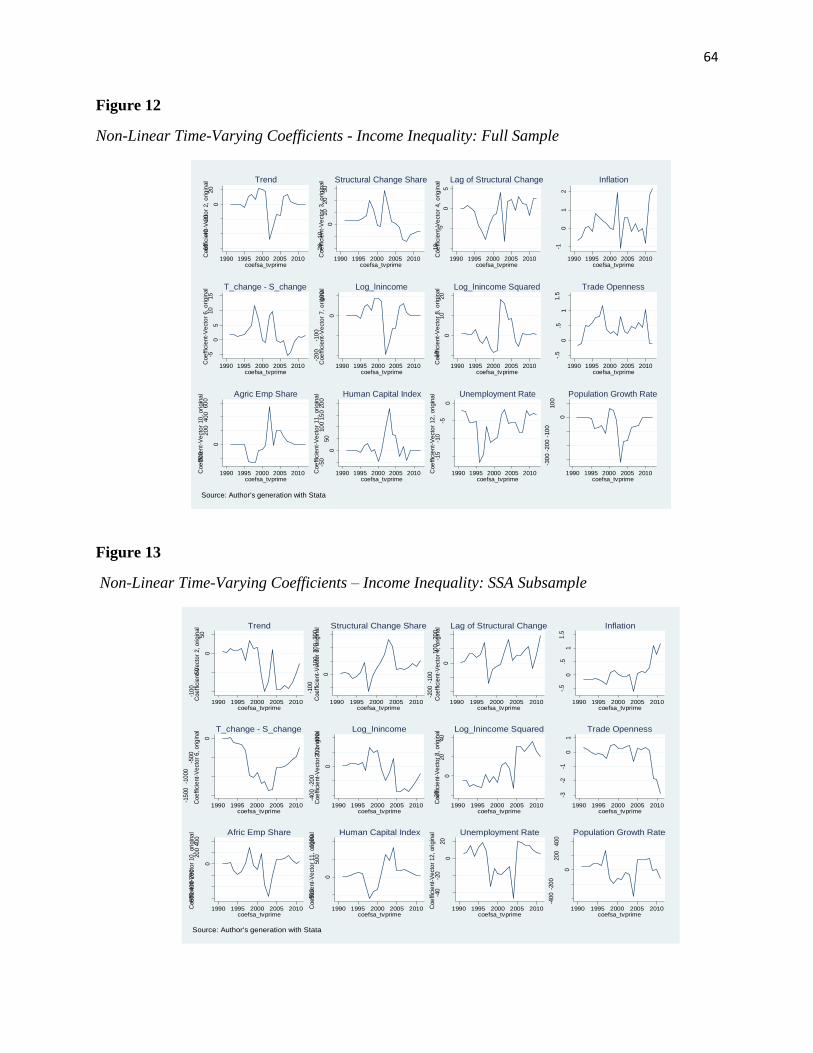
64

Figure 12

Non-Linear Time-Varying Coefficients - Income Inequality: Full Sample

Figure 13

Non-Linear Time-Varying Coefficients – Income Inequality: SSA Subsample

-60

-40

-20

020

Coe

ffic

ient-

Ve

cto

r 1,

orig

inal

1990 1995 2000 2005 2010coefsa_tvprime

Trend

-20

-10

010

20

30

Coe

ffic

ient-

Ve

cto

r 2,

orig

inal

1990 1995 2000 2005 2010coefsa_tvprime

Structural Change Share

-10

-50

5

Coe

ffic

ient-

Ve

cto

r 3,

orig

inal

1990 1995 2000 2005 2010coefsa_tvprime

Lag of Structural Change

-10

12

Coe

ffic

ient-

Ve

cto

r 4,

orig

inal

1990 1995 2000 2005 2010coefsa_tvprime

Inflation

-50

510

15

Coe

ffic

ient-

Ve

cto

r 5,

orig

inal

1990 1995 2000 2005 2010coefsa_tvprime

T_change - S_change

-20

0-1

00

0

10

0

Coe

ffic

ient-

Ve

cto

r 6,

orig

inal

1990 1995 2000 2005 2010coefsa_tvprime

Log_lnincome

-10

010

20

Coe

ffic

ient-

Ve

cto

r 7,

orig

inal

1990 1995 2000 2005 2010coefsa_tvprime

Log_lnincome Squared

-.5

0.5

11.5

Coe

ffic

ient-

Ve

cto

r 8,

orig

inal

1990 1995 2000 2005 2010coefsa_tvprime

Trade Openness

-20

0

0

20

040

060

0

Coe

ffic

ient-

Ve

cto

r 9,

orig

inal

1990 1995 2000 2005 2010coefsa_tvprime

Agric Emp Share

-50

050

10

015

020

0

Coe

ffic

ient-

Ve

cto

r 10

, ori

gin

al

1990 1995 2000 2005 2010coefsa_tvprime

Human Capital Index

-15

-10

-50

Coe

ffic

ient-

Ve

cto

r 11

, ori

gin

al

1990 1995 2000 2005 2010coefsa_tvprime

Unemployment Rate

-30

0-2

00

-10

0

0

10

0

Coe

ffic

ient-

Ve

cto

r 12

, ori

gin

al

1990 1995 2000 2005 2010coefsa_tvprime



-10

0-5

0

050

Coe

ffic

ient-

Ve

cto

r 1,

orig

inal

1990 1995 2000 2005 2010coefsa_tvprime

Trend

-10

0

0

10

020

030

0

Coe

ffic

ient-

Ve

cto

r 2,

orig

inal

1990 1995 2000 2005 2010coefsa_tvprime


-20

0-1

00

0

10

020

0

Coe

ffic

ient-

Ve

cto

r 3,

orig

inal

1990 1995 2000 2005 2010coefsa_tvprime


-.5

0.5

11.5

Coe

ffic

ient-

Ve

cto

r 4,

orig

inal

1990 1995 2000 2005 2010coefsa_tvprime

Inflation

-15

00

-10

00

-50

0

0

Coe

ffic

ient-

Ve

cto

r 5,

orig

inal

1990 1995 2000 2005 2010coefsa_tvprime

T_change - S_change

-40

0-2

00

0

20

040

0

Coe

ffic

ient-

Ve

cto

r 6,

orig

inal

1990 1995 2000 2005 2010coefsa_tvprime

Log_lnincome

-20

020

40

Coe

ffic

ient-

Ve

cto

r 7,

orig

inal

1990 1995 2000 2005 2010coefsa_tvprime


-3-2

-10

1

Coe

ffic

ient-

Ve

cto

r 8,

orig

inal

1990 1995 2000 2005 2010coefsa_tvprime

Trade Openness

-60

0-4

00-2

00

0

20

040

0

Coe

ffic

ient-

Ve

cto

r 9,

orig

inal

1990 1995 2000 2005 2010coefsa_tvprime

Afric Emp Share

-50

0

0

50

010

00

Coe

ffic

ient-

Ve

cto

r 10

, ori

gin

al

1990 1995 2000 2005 2010coefsa_tvprime

Human Capital Index

-40

-20

020

Coe

ffic

ient-

Ve

cto

r 11

, ori

gin

al

1990 1995 2000 2005 2010coefsa_tvprime

Unemployment Rate

-40

0-2

00

0

20

040

0

Coe

ffic

ient-

Ve

cto

r 12

, ori

gin

al

1990 1995 2000 2005 2010coefsa_tvprime



65

Figure 14 presents the results for the Asian subsample. We see that structural change

reduces income inequality for most of the period from 1990 to 2005; the negative effect is reversed

after that period. However, the lagged value of structural change widens income inequality for

most of the period, even though the effect gets smaller after 2005. Inflation and the difference

between technical change and structural change both have negative effects for some years and

positive effects for other years. The log of income is found to reduce income inequality for most

of the period, while the squared term increases income inequality. Trade openness, the agricultural

employment shares, and human capital all widen income inequality for most of the years.

Unemployment and population growth have negative effects for some years and positive effects

for others. Again, the changes in sign of the coefficients over time suggest nonlinearities

Figure 14

Non-Linear Time-Varying Coefficients - Income Inequality: Asian Subsample

-60

-40

-20

020

Coe

ffic

ient-

Ve

cto

r 1,

orig

inal

1990 1995 2000 2005 2010coefsa_tvprime

Trend

-30

0-20

0-10

0

0

10

020

0

Coe

ffic

ient-

Ve

cto

r 2,

orig

inal

1990 1995 2000 2005 2010coefsa_tvprime


0

10

020

030

040

0

Coe

ffic

ient-

Ve

cto

r 3,

orig

inal

1990 1995 2000 2005 2010coefsa_tvprime

Lag of Structural Change-1

01

23

Coe

ffic

ient-

Ve

cto

r 4,

orig

inal

1990 1995 2000 2005 2010coefsa_tvprime

Inflation

-20

24

6

Coe

ffic

ient-

Ve

cto

r 5,

orig

inal

1990 1995 2000 2005 2010coefsa_tvprime

T_change - S_change

-30

0-2

00

-10

0

0

10

0

Coe

ffic

ient-

Ve

cto

r 6,

orig

inal

1990 1995 2000 2005 2010coefsa_tvprime

Log_lnincome

-10

010

20

30

Coe

ffic

ient-

Ve

cto

r 7,

orig

inal

1990 1995 2000 2005 2010coefsa_tvprime


-.5

0.5

1

Coe

ffic

ient-

Ve

cto

r 8,

orig

inal

1990 1995 2000 2005 2010coefsa_tvprime

Trade Openness

0

10

020

030

0

Coe

ffic

ient-

Ve

cto

r 9,

orig

inal

1990 1995 2000 2005 2010coefsa_tvprime

Agric Emp Share

-10

0

0

10

020

030

0

Coe

ffic

ient-

Ve

cto

r 10

, ori

gin

al

1990 1995 2000 2005 2010coefsa_tvprime

Human Capital Index

-20

-15

-10

-50

5

Coe

ffic

ient-

Ve

cto

r 11

, ori

gin

al

1990 1995 2000 2005 2010coefsa_tvprime

Unemployment Rate

-40

0-3

00-

20

0-1

00

0

10

0

Coe

ffic

ient-

Ve

cto

r 12

, ori

gin

al

1990 1995 2000 2005 2010coefsa_tvprime



66

5.2.3 Poverty

This section presents the results for poverty as a dependent variable. Figure 15 presents the

results for the full sample. Structural change has a positive coefficient for most of the years. This

implies that structural change reduces poverty by increasing household per capita consumption.

The lagged value of structural change also increases household per capita consumption for some

years and reduces it for others. Inflation has negative effects on household consumption for some

years and positive effects for others. The difference between technical change and structural

change generally increases household consumption. However, the coefficients are negative for

some of the years as well. The log of income generally reduces household consumption while the

squared term increases it. Trade openness has a negative effect on household consumption for

some of the years and a positive effect on other years. The agricultural employment share and

human capital also have negative effects on household consumption for some years and positive

for other years. Unemployment unexpectedly has negative coefficients for some of the years. Other

years, however, have positive coefficients as expected. Population growth also increases

household consumption per capita, which is unexpected.

Figure 16 presents the results for the SSA subsample. The coefficients of structural change

are positive for some years and negative for others. The lagged value of structural change also

increases household consumption expenditure for some years and reduces it for other years.

Inflation worsens poverty by reducing household consumption expenditure. The difference

between technical change and structural change reduces poverty by increasing household

consumption expenditure for some years but has the opposite effect in other years. The coefficients

of the log of income are positive for some years and negative for others, while the coefficients of

the squared term are again mirror images of that of the log of income

67

Figure 15

Non-Linear Time-Varying Coefficients - Poverty: Full Sample

Trade openness and agricultural employment share reduce poverty by increasing household

consumption expenditure. Human capital, unemployment, and population growth increase poverty

for some years and reduce it for other years. The graphs suggest the existence of some

nonlinearities.

Lastly, Figure 17 presents the results for the Asian subsample of countries. The coefficients

of structural change are found to be negative for some years and positive for other years. The

coefficients of the lagged value of structural change are also positive for some years and negative

for others. The coefficients of inflation are negative for all years. The difference between technical

change and structural change also has negative coefficients for some years and positive effects for

-10

00

0-8

000-6

000-4

000-2

000

0

Coe

ffic

ient-

Ve

cto

r 1,

orig

inal

1990 1995 2000 2005 2010coefsa_tvprime

Trend

020

40

60

80

Coe

ffic

ient-

Ve

cto

r 2,

orig

inal

1990 1995 2000 2005 2010coefsa_tvprime


-20

-10

010

Coe

ffic

ient-

Ve

cto

r 3,

orig

inal

1990 1995 2000 2005 2010coefsa_tvprime


-.3

-.2

-.1

0.1

.2

Coe

ffic

ient-

Ve

cto

r 4,

orig

inal

1990 1995 2000 2005 2010coefsa_tvprime

Inflation-2

0

020

40

Coe

ffic

ient-

Ve

cto

r 5,

orig

inal

1990 1995 2000 2005 2010coefsa_tvprime

T_change - S_change-1

000 -8

00-

60

0-40

0-20

0

0

Coe

ffic

ient-

Ve

cto

r 6,

orig

inal

1990 1995 2000 2005 2010coefsa_tvprime

Log_income

0

20

004

0006

0008

00010

00

0

Coe

ffic

ient-

Ve

cto

r 7,

orig

inal

1990 1995 2000 2005 2010coefsa_tvprime

Log_income Squared

-.4

-.2

0.2

.4

Coe

ffic

ient-

Ve

cto

r 8,

orig

inal

1990 1995 2000 2005 2010coefsa_tvprime

Trade Openness

-30

0-20

0-10

0

0

10

020

0

Coe

ffic

ient-

Ve

cto

r 9,

orig

inal

1990 1995 2000 2005 2010coefsa_tvprime

Agric Emp Share

-60

0-4

00

-20

0

0

20

0

Coe

ffic

ient-

Ve

cto

r 10

, ori

gin

al

1990 1995 2000 2005 2010coefsa_tvprime

Human Capital Index

-10

010

20

30

Coe

ffic

ient-

Ve

cto

r 11

, ori

gin

al

1990 1995 2000 2005 2010coefsa_tvprime

Unemployment Rate

-10

0

0

10

020

030

0

Coe

ffic

ient-

Ve

cto

r 12

, ori

gin

al

1990 1995 2000 2005 2010coefsa_tvprime


Source: Author's generation using Stata

68

other years. The coefficients for the log of income are generally negative while the squared term

generally has positive coefficients.

Figure 16

Non-Linear Time-Varying Coefficients - Poverty: SSA Subsample

Trade openness has negative coefficients for most of the years, implying that trade

openness worsens poverty. The coefficients of the agricultural employment share are also negative

for some years and positive for others. The negative coefficients occur for earlier years while the

positive effects occur for latter years. Also, earlier coefficients of human capital are positive, while

the latter years have negative coefficients. The coefficients of the unemployment rate are generally

negative. The population growth rate mostly has positive coefficients, which is unexpected.

Again, the change in signs of the coefficients over time suggests the existence of

nonlinearities in the relationships being estimated.

-20

00

0

20

00

40

00

60

00

Coe

ffic

ient-

Ve

cto

r 1,

orig

inal

1990 1995 2000 2005 2010coefsa_tvprime

Trend

-15

0-1

00

-50

050

Coe

ffic

ient-

Ve

cto

r 2,

orig

inal

1990 1995 2000 2005 2010coefsa_tvprime


-50

050

10

0

Coe

ffic

ient-

Ve

cto

r 3,

orig

inal

1990 1995 2000 2005 2010coefsa_tvprime


-.7

-.6

-.5

-.4

-.3

-.2

Coe

ffic

ient-

Ve

cto

r 4,

orig

inal

1990 1995 2000 2005 2010coefsa_tvprime

Inflation

-40

0-3

00-2

00-1

00

0

10

0

Coe

ffic

ient-

Ve

cto

r 5,

orig

inal

1990 1995 2000 2005 2010coefsa_tvprime

T_change - S_change

-20

0

0

20

040

060

0

Coe

ffic

ient-

Ve

cto

r 6,

orig

inal

1990 1995 2000 2005 2010coefsa_tvprime

Log_income

-40

00

-20

00

0

20

00

Coe

ffic

ient-

Ve

cto

r 7,

orig

inal

1990 1995 2000 2005 2010coefsa_tvprime

Log_income Squared

0.2

.4.6

Coe

ffic

ient-

Ve

cto

r 8,

orig

inal

1990 1995 2000 2005 2010coefsa_tvprime

Trade Openness

0

10

020

030

040

0

Coe

ffic

ient-

Ve

cto

r 9,

orig

inal

1990 1995 2000 2005 2010coefsa_tvprime

Agric Emp Share

-50

050

10

015

0

Coe

ffic

ient-

Ve

cto

r 10

, ori

gin

al

1990 1995 2000 2005 2010coefsa_tvprime

Human Capital Index

-10

12

3

Coe

ffic

ient-

Ve

cto

r 11

, ori

gin

al

1990 1995 2000 2005 2010coefsa_tvprime

Unemployment Rate

-40

-30

-20

-10

010

Coe

ffic

ient-

Ve

cto

r 12

, ori

gin

al

1990 1995 2000 2005 2010coefsa_tvprime



69

Table 17

Non-Linear Time-Varying Coefficients - Poverty: Asian Subsample

-40

00

0-30

00

0 -20

00

0-10

00

0

0

Coe

ffic

ient-

Ve

cto

r 1,

orig

inal

1990 1995 2000 2005 2010coefsa_tvprime

Trend

-50

050

10

015

020

0

Coe

ffic

ient-

Ve

cto

r 2,

orig

inal

1990 1995 2000 2005 2010coefsa_tvprime


-20

0

0

20

040

060

0

Coe

ffic

ient-

Ve

cto

r 3,

orig

inal

1990 1995 2000 2005 2010coefsa_tvprime


-1-.

50

.51

Coe

ffic

ient-

Ve

cto

r 4,

orig

inal

1990 1995 2000 2005 2010coefsa_tvprime

Inflation

-20

24

6

Coe

ffic

ient-

Ve

cto

r 5,

orig

inal

1990 1995 2000 2005 2010coefsa_tvprime

T_change - S_change

-40

00-

30

00-

20

00-10

00

0

Coe

ffic

ient-

Ve

cto

r 6,

orig

inal

1990 1995 2000 2005 2010coefsa_tvprime

Log_income

0

10

00

020

00

030

00

040

00

0

Coe

ffic

ient-

Ve

cto

r 7,

orig

inal

1990 1995 2000 2005 2010coefsa_tvprime

Log_income Squared

-2-1

.5-1

-.5

0

Coe

ffic

ient-

Ve

cto

r 8,

orig

inal

1990 1995 2000 2005 2010coefsa_tvprime

Trade Openness

-50

050

10

015

020

0

Coe

ffic

ient-

Ve

cto

r 9,

orig

inal

1990 1995 2000 2005 2010coefsa_tvprime

Agric Emp Share

-60

0-40

0-20

0

0

20

040

0

Coe

ffic

ient-

Ve

cto

r 10

, ori

gin

al

1990 1995 2000 2005 2010coefsa_tvprime

Human Capital Index

-30

-20

-10

010

Coe

ffic

ient-

Ve

cto

r 11

, ori

gin

al

1990 1995 2000 2005 2010coefsa_tvprime

Unemployment Rate

-10

0

0

10

020

030

0

Coe

ffic

ient-

Ve

cto

r 12

, ori

gin

al

1990 1995 2000 2005 2010coefsa_tvprime



70

Chapter Six

6.1 Summary and Findings

The focus of this study is to determine the relationships between structural change, poverty,

and inequality. Specifically, the study seeks to determine if shifts in labor shares in productivity

growth affect poverty and inequality. Economic growth, especially in developing countries, has

seen a significant surge in recent times. This is mainly due to structural transformations that these

economies are undergoing. However, concerns have been raised about the rising inequality that

has coincided with the significant expansion in economic growth. This justifies the need to

undertake a study into the effects of this structural change on poverty and inequality. Structural

change is studied in line with Lewis's (1954) two-sector model which concentrates on intersectoral

labor movements as the economy undergoes a significant structural transformation. The

relationship between structural change and inequality is then assessed based on the Kuznets (1955)

hypothesis that establishes an inverted U-shaped relationship between economic growth (that is

induced by structural change) and inequality.

Though some studies have explored the relationship between structural change and

inequality, no known study has measured structural change by looking at shifts in labor shares in

productivity growth, the direction this study takes; hence, this research is significantly different

from other studies in this area. The study covers a sample of 28 countries all over the world with

a focus on Asia and Sub-Sharan Africa. The sample contains seven European countries, seven

Asian countries, four Latin American countries, and ten sub-Saharan African countries.

Estimations are first done for the full sample and then for the Asian and sub-Saharan African

subsamples. The dataset ranges from 1963 to 2012.

71

Productivity growth decomposition is done following McMillan & Rodrik (2011). This

procedure decomposes productivity growth into the part that is due to structural change and the

part that is due to technical change. Three dependent variables are specified; industrial wage

inequality, income inequality, and the percentage change in household consumption per capita (as

a measure of poverty). Parametric estimation techniques are first employed. Specifically, pooled

OLS, fixed effects, and random effects estimation techniques are applied. The Hausman test is

used to determine the most preferred model between the fixed and random-effects models. In all

regressions, the fixed effects model is the most preferred. The results for the parametric estimations

show that overall, structural change or a shift in labor shares in productivity growth reduces

industrial wage inequality, income inequality, and poverty. This is true for the full sample as well

for Asian and sub-Saharan African subsamples.

To take the analysis further, the study also employs nonparametric estimation techniques.

This route is taken to explore the possibility of nonlinearities in the functional relationships

between the dependent and independent variables. The fixed effect time-varying coefficients

technique espoused by Li et al. (2011) is utilized. The results show that the effects of structural

change on poverty and inequality are likely nonlinear. This is because the time-varying coefficients

are found to be positive for some years and negative for others. This situation is the same for most

of the control variables. To ensure robustness, robust standard errors are produced for all

estimations.

The main findings of the research can be summarized as follows:

• Generally, Structural change (measured as productivity growth induced by intersectoral

labor movements) reduces inequality and poverty. Both income inequality and wage

72

inequalities are significantly reduced in response to shifts in labor shares in productivity

growth.

• Structural change has a dynamic effect on poverty and inequality. This is because the

lagged value of structural change is found to also reduce inequality and poverty. In some

cases, only the coefficient of the lagged value is statistically significant. This finding

implies that the effects of structural change on inequality and poverty may take time to

manifest. Hence current intersectoral labor movements can affect inequality and poverty

in future periods.

• Structural change significantly reduces industrial wage inequality for both Asian and sub-

Sharan African countries. However, the effects are stronger for Asian countries than for

Sub-Saharan African countries

• There is evidence that structural change reduces income inequality for Asia. No such

evidence is found for SSA.

• Structural change significantly reduces poverty for SSA. There is no such evidence for

Asia.

• Inflation generally exacerbates inequality and poverty for both SSA and Asia. This is

expected as higher inflation affects living standards.

• Trade openness has no significant effect on inequality and poverty. This finding is the same

for both SSA and Asia. This finding is against the general notion that trade openness

increases wealth, which translates into reduced poverty and inequality.

• The agricultural employment share plays a significant role in reducing industrial wage

inequality and income inequality for sub-Saharan Africa. This further highlights the

importance of the agricultural sector in sub-Saharan Africa.

73

• Improvements in human capital induce industrial wage inequalities for both Asia and Sub-

Saharan Africa. For Asia, human capital also significantly widens income inequality.

However, there are no significant effects on poverty.

• Unemployment and population growth also generally widen poverty and inequality.

• Nonlinearities exist in the relationship between structural change, inequality, and poverty.

6.2 Recommendations.

Based on the findings of the study, the following recommendations are made for policy

purposes and further research.

• Having found that shifts in labor shares in productivity growth significantly reduces

poverty and inequality, the study recommends that policies aimed at improving the quality

of labor should be strongly encouraged in developing countries.

• Inflation stabilization should be given priority in developing countries as a means of

improving the quality of life of these countries.

• The agricultural sector in developing countries, especially for sub-Saharan Africa, should

be given much attention. Increasing employment in this sector is identified as a significant

means of reducing poverty and inequality in this sub-region.

• Attention should be given to the effect of trade openness on poverty and inequality in

developing countries. Developing countries may not be gaining as much from trade, thus a

major restructuring process should be put in place to ensure that developing countries

leverage the opportunities that trade openness offers.

• Reducing unemployment and managing population growth should also be given priority in

developing countries because these factors were found to increase poverty and inequality.

74

• The study found that nonlinearities may exist in the relationships estimated. Hence, in

future research, it is recommended that nonlinear estimation techniques be employed to

further provide more insight into the nature of these relationships.

• The effect of structural change on poverty and inequality is dynamic rather than static.

Hence, dynamic panel data estimation techniques should also be considered in further

research.

6.3 Limitations

Even though the study was generally successful, some limitations were encountered. Chief

among them was the lack of sufficient data for some of the countries. Because the study mainly

depends on the productivity decomposition process, the number of countries used is limited to the

countries available on the GGDC 10-sector database. Since the dataset contains only 28 countries,

more countries could not be added because data on value-added and employment shares for these

10 sectors could not be obtained elsewhere. Separate regressions could not be made for Latin

America because of the small sample of Latin American countries. More countries captured would

have provided more robust estimators than those obtained. Again, data were missing for some of

the years for some countries, producing an unbalanced panel. This limited the estimation process,

especially for the nonparametric estimations which generally require a balanced panel. The

estimations were done for only the years that the data were complete. Also, because of the

unbalanced panel and insufficient data, other nonparametric options such as bootstrapping (which

could have produced better estimates of the coefficient functions) could not be conducted.

Despite the data limitations, the study still produced relevant results that can inform policy-

making and provoke further research.

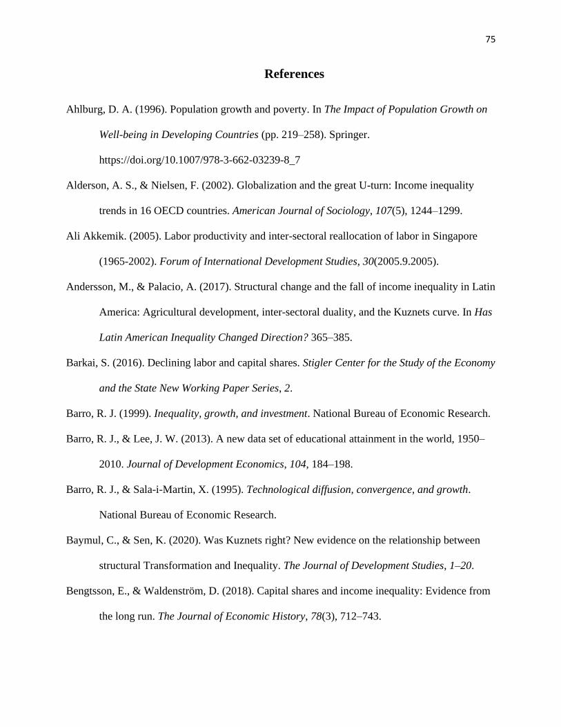
75

References

Ahlburg, D. A. (1996). Population growth and poverty. In The Impact of Population Growth on

Well-being in Developing Countries (pp. 219–258). Springer.

https://doi.org/10.1007/978-3-662-03239-8_7

Alderson, A. S., & Nielsen, F. (2002). Globalization and the great U-turn: Income inequality

trends in 16 OECD countries. American Journal of Sociology, 107(5), 1244–1299.

Ali Akkemik. (2005). Labor productivity and inter-sectoral reallocation of labor in Singapore

(1965-2002). Forum of International Development Studies, 30(2005.9.2005).

Andersson, M., & Palacio, A. (2017). Structural change and the fall of income inequality in Latin

America: Agricultural development, inter-sectoral duality, and the Kuznets curve. In Has

Latin American Inequality Changed Direction? 365–385.

Barkai, S. (2016). Declining labor and capital shares. Stigler Center for the Study of the Economy

and the State New Working Paper Series, 2.

Barro, R. J. (1999). Inequality, growth, and investment. National Bureau of Economic Research.

Barro, R. J., & Lee, J. W. (2013). A new data set of educational attainment in the world, 1950–

2010. Journal of Development Economics, 104, 184–198.

Barro, R. J., & Sala-i-Martin, X. (1995). Technological diffusion, convergence, and growth.

National Bureau of Economic Research.

Baymul, C., & Sen, K. (2020). Was Kuznets right? New evidence on the relationship between

structural Transformation and Inequality. The Journal of Development Studies, 1–20.

Bengtsson, E., & Waldenström, D. (2018). Capital shares and income inequality: Evidence from

the long run. The Journal of Economic History, 78(3), 712–743.

76

Beqiraj, E., Fanti, L., & Zamparelli, L. (2018). Structural Change and the Wage Share: A Two-

Sector Kaleckian Model [MPRA Paper]. https://mpra.ub.uni-muenchen.de/89558/

Bolt, J., Lensink, R., & Raster, T. (2017). Structural transformation and inequality in Africa: An

investigation into the Kuznets curve. Groningen: University of Groningen.

Carmignani, F., & Mandeville, T. (2014). Never been industrialized: A tale of African structural

change. Structural Change and Economic Dynamics, 31, 124–137.

Chen, S., Jefferson, G. H., & Zhang, J. (2011). Structural change, productivity growth, and

industrial transformation in China. China Economic Review, 22(1), 133–150.

Clark, C. (Wirtschaftswissenschaftler). (1957). The conditions of economic progress.

Credit Suisse, A. (2014). Global wealth report 2014.

Dabla-Norris, M. E., Kochhar, M. K., Suphaphiphat, M. N., Ricka, M. F., & Tsounta, E. (2015).

Causes and consequences of income inequality: A global perspective. International

Monetary Fund.

Dartanto, T., Yuan, E. Z. W., & Sofiyandi, Y. (2016). Structural transformation and the

dynamics of income equality in Indonesia: 1996–2014. Kuznets Beyond Kuznets, 171–

185.

Deininger, K., & Squire, L. (1996). A new data set measuring income inequality. The World

Bank Economic Review, 10(3), 565–591. https://doi.org/10.1093/wber/10.3.565

Dreher, A., & Gaston, N. (2008). Has globalization increased inequality?. Review of

International Economics, 16(3), 516–536. https://doi.org/10.1111/j.1467-

9396.2008.00743.x

77

Echevarria, C. (1997). Changes in sectoral composition associated with economic growth.

International Economic Review, 38(2), 431–452. JSTOR.

https://doi.org/10.2307/2527382

Fagerberg, J. (2000). Technological progress, structural change, and productivity growth: A

comparative study. Structural Change and Economic Dynamics, 11(4), 393–411.

Fan, S., Zhang, X., & Robinson, S. (2003). Structural change and economic growth in China.

Review of Development Economics, 7(3), 360–377. https://doi.org/10.1111/1467-

9361.00196

Fields, G. S. (2004). Dualism in the labor market: A perspective on the Lewis model after half a

century. The Manchester School, 72(6), 724–735. https://doi.org/10.1111/j.1467-

9957.2004.00432.x

Galbraith, J. K., Halbach, B., Malinowska, A., Shams, A., & Zhang, W. (2015). The UTIP

Global Inequality Datasets, 1963-2008 (No. 2015/019). WIDER Working Paper.

https://doi.org/10.35188/UNU-WIDER/2015/904-6

Goesling, B. (2001). Changing income inequalities within and between nations: New evidence.

American Sociological Review, 66(5), 745–761. JSTOR. https://doi.org/10.2307/3088956

Green, W. H. (2008). Handbook of econometrics. Applied Econometrics, 2, 413–556.

Grossman, G. M., Helpman, E., Oberfield, E., & Sampson, T. (2017). The Productivity

Slowdown and the Declining Labor Share: A Neoclassical Exploration (Working Paper

No. 23853). National Bureau of Economic Research. https://doi.org/10.3386/w23853

Hub, I. S. K. (n.d.). UNDP Report Discusses Inequality in Developing Countries | News | SDG

Knowledge Hub | IISD. Retrieved November 27, 2019, from

http://sdg.iisd.org/news/undp-report-discusses-inequality-in-developing-countries/

78

Jacobson, M., & Occhino, F. (2012). Labor’s declining share of income and rising inequality.

Economic Commentary, 2012–13. https://www.clevelandfed.org/newsroom-and-

events/publications/economic-commentary/economic-commentary-archives/2012-

economic-commentaries/ec-201213-labors-declining-share-of-income-and-rising-

inequality

Jain-Chandra, S., Kinda, T., Kochhar, K., Piao, S., & Schauer, J. (2016). Sharing the growth

dividend: analysis of inequality in Asia. IMF Working Paper, 16(48).

Kai, H., & Hamori, S. (2009). Globalization, financial depth, and inequality in Sub-Saharan

Africa. Economics Bulletin, 29(3), 2025–2037.

Kanbur, Z. J. R. (2013). Confronting rising inequality in Asia. Nankai Economic Studies, 1.

Karabarbounis, L., & Neiman, B. (2012). Declining labor shares and the global rise of corporate

saving (Working Paper No. 18154). National Bureau of Economic Research.

https://doi.org/10.3386/w18154

Kilic, C. (2015). Effects of globalization on economic growth: Panel data analysis for developing

countries. Petroleum-Gas University of Ploiesti Bulletin, Technical Series, 67(1).

Klasen, S., Scholl, N., Lahoti, R., Ochmann, S., & Vollmer, S. (2016). Inequality-worldwide

trends and current debates (No. 209). Courant Research Centre: Poverty, Equity, and

Growth-Discussion Papers.

Kum, H. (2008). Inequality and structural change. University of Texas Inequality Project

Working Paper, 54.

Kuznets, S. (1965). Economic growth and structural change. Nueva York: Norton.

Kuznets, S. (1955). Economic growth and income inequality. The American Economic Review,

45(1), 1–28.

79

Laitner, J. (2000). Structural change and economic growth. The Review of Economic Studies,

67(3), 545–561.

Lewis, W. A. (1954). Economic development with unlimited supplies of labor. The Manchester

School, 22(2), 139–191.

Li, D., Chen, J., & Gao, J. (2011). Non-parametric time-varying coefficient panel data models

with fixed effects. The Econometrics Journal, 14(3), 387–408.

Li, S., Gong, L., & Pan, S. (2016). Structural change and economic growth.

Lundberg, M., & Squire, L. (2003). The simultaneous evolution of growth and inequality. The

Economic Journal, 113(487), 326–344.

McMillan, M. S., & Rodrik, D. (2011). Globalization, structural change, and productivity

growth. National Bureau of Economic Research.

Nissanke, M., & Thorbecke, E. (2010). Globalization, poverty, and inequality in Latin America:

Findings from case studies. World Development, 38(6), 797–802.

https://doi.org/10.1016/j.worlddev.2010.02.003

Park, D., Lee, M., & Aizenman, J. (2014). Structural change and inequality: A conceptual

overview with reference to developing Asia. In Inequality in Asia and the Pacific (pp.

158–179). Routledge.

Paul, S. (2016). Structural transformation, growth incidence, and inequality. DECRG Kuala

Lumpur Seminar Series.

Peneder, M. (2002). Structural change and aggregate growth. Structural Change and Economic

Dynamics, 14, 427–448.

Piketty, T. (2015). About capital in the twenty-first century. American Economic Review, 105(5),

48–53.

80

Psacharopoulos, G. (1994). Returns to investment in education: A global update. World

Development, 22(9), 1325–1343. https://doi.org/10.1016/0305-750X(94)90007-8

Ravallion, M. (2014). Income inequality in the developing world. Science, 344(6186), 851–855.

Rodrik, D. (1997). Has Globalization Gone Too Far? Number 57 in Peterson Institute Press.

Rostow, W. W. (1971). Politics and the stages of growth. Cambridge University Press.

https://ideas.repec.org/b/cup/cbooks/9780521096539.html

Roy, R. P., & Roy, S. S. (2017). Structural change, trade, and inequality: Some cross-country

evidence (No. 763). ADBI Working Paper Series.

Samimi, P., & Jenatabadi, H. S. (2014). Globalization and economic growth: Empirical evidence

on the role of complementarities. PLOS ONE, 9(4), e87824.

https://doi.org/10.1371/journal.pone.0087824

Schultz, T. P. (1998). Inequality in the distribution of personal income in the world: How it is

changing and why. Journal of Population Economics, 11(3), 307–344.

Signor, D., Kim, J., & Tebaldi, E. (2019). Persistence and determinants of income inequality:

The Brazilian case. Review of Development Economics, 23(4), 1748–1767.

https://doi.org/10.1111/rode.12598

Syrquin, M. (1988). Patterns of structural change. Handbook of Development Economics, 1, 203–

273.

Teixeira, A. A., & Queirós, A. S. (2016). Economic growth, human capital, and structural

change: A dynamic panel data analysis. Research Policy, 45(8), 1636–1648.

Torres-Reyna, O. (2007). Panel data analysis fixed and random effects using Stata (v. 4.2). Data

& Statistical Services, Princeton University.

81

Visaria, P. (1981). Poverty and unemployment in India: An analysis of recent evidence. World

Development, 9(3), 277–300. https://doi.org/10.1016/0305-750X(81)90031-0

Vries, G. de, Timmer, M., & Vries, K. de. (2014). Patterns of structural change in developing

countries. Groningen Growth and Development Centre, University of Groningen.

Vu, K. M. (2017). Structural change and economic growth: Empirical evidence and policy

insights from Asian economies. Structural Change and Economic Dynamics, 41, 64–77.

Wan, G., Wang, C., & Zhang, X. (2016). Structural change and income distribution: Accounting

for regional inequality in the People’s Republic of China and its changes from 1952–

2012.

Williamson, J. G. (1997). Globalization and inequality, past, and present. The World Bank

Research Observer, 12(2), 117–135. https://doi.org/10.1093/wbro/12.2.117

Yatchew, A. (1998). Nonparametric regression techniques in economics. Journal of Economic

Literature, 36(2), 669–721.

Yay, G., Taştan, H., & Oktayer, A. (2016). Globalization, economic freedom, and wage

inequality: A panel data analysis. Panoeconomicus, 63(5), 581–601.

https://doi.org/10.2298/PAN130515024Y

Ying, Y.-H., Chang, K., & Lee, C.-H. (2014). 2. The impact of globalization on economic

growth. Romanian Journal of Economic Forecasting, 10.

Zhu, S. C., & Trefler, D. (2005). Trade and inequality in developing countries: A general

equilibrium analysis. Journal of International Economics, 65(1), 21–48.

82

Documents

Do Shifts in Labor Shares in Productivity Growth Affect