NBER WORKING PAPER SERIES

DO MEASURES OF FINANCIAL CONSTRAINTS MEASURE FINANCIAL CONSTRAINTS?

Joan Farre-MensaAlexander Ljungqvist

Working Paper 19551http://www.nber.org/papers/w19551

NATIONAL BUREAU OF ECONOMIC RESEARCH1050 Massachusetts Avenue

Cambridge, MA 02138October 2013

We are grateful to seminar audiences at HBS, NYU, NCCU, and the IDC Summer Finance Conferencefor their comments. Ljungqvist gratefully acknowledges the generous hospitality of Harvard BusinessSchool while working on this project. The views expressed herein are those of the authors and do notnecessarily reflect the views of the National Bureau of Economic Research.

NBER working papers are circulated for discussion and comment purposes. They have not been peer-reviewed or been subject to the review by the NBER Board of Directors that accompanies officialNBER publications.

© 2013 by Joan Farre-Mensa and Alexander Ljungqvist. All rights reserved. Short sections of text,not to exceed two paragraphs, may be quoted without explicit permission provided that full credit,including © notice, is given to the source.

Do Measures of Financial Constraints Measure Financial Constraints?Joan Farre-Mensa and Alexander LjungqvistNBER Working Paper No. 19551October 2013JEL No. G31,G32,G33

ABSTRACT

Financial constraints are not directly observable, so empirical research relies on indirect measures.We evaluate how well five popular measures (paying dividends, having a credit rating, and the Kaplan-Zingales, Whited-Wu, and Hadlock-Pierce indices) identify firms that are financially constrained,using three novel tests: an exogenous increase in a firm’s demand for credit; exogenous variation inthe supply of bank loans; and the tendency for firms to pay out the proceeds of equity issues to theirshareholders (“equity recycling”). We find that none of the five measures identifies firms that behaveas if they were constrained: public firms classified as constrained have no trouble raising debt whentheir demand for debt increases, are unaffected by changes in the supply of bank loans, and engagein equity recycling. The point estimates are little different for supposedly constrained and unconstrainedfirms, even though we find important differences in their characteristics and sources of financing. Onthe other hand, privately held firms (particularly small ones) and public firms with below investment-grade ratings appear to be financially constrained.

Joan Farre-MensaHarvard Business SchoolRock Center 218Boston, MA 02163jfarremensa@hbs.edu

Alexander LjungqvistStern School of BusinessNew York University44 West Fourth Street, #9-160New York, NY 10012and NBERaljungqv@stern.nyu.edu

1

How financial constraints affect firm behavior is a core question in corporate finance.1

Answering it requires a way to identify constrained firms with reasonable accuracy. Since the

financial constraints a firm faces are not directly observable, the empirical literature finds itself

having to rely on indirect proxies (such as having a credit rating or paying dividends) or on one

of three popular indices based on linear combinations of observable firm characteristics such as

size, age, or leverage (the Kaplan-Zingales, Whited-Wu, and Hadlock-Pierce indices).

In this paper, we ask a simple question: How well do these measures of financial constraints

identify firms that are plausibly financially constrained? The short answer is: not well at all.

Our empirical strategy is based on the premise that firms that are financially constrained

effectively face an inelastic supply of external capital: raising external capital quickly becomes

ever more expensive (reflecting a steep supply curve) and in the limit the firm is shut out of the

capital markets (a vertical supply curve).2 In contrast, firms that can raise a large amount of

external capital without much of an increase in the cost of capital are plausibly unconstrained.

We propose three tests to identify the shape of a firm’s supply of capital curve. The

traditional way to estimate a supply curve is to exploit exogenous variation in demand. This is

precisely what our first test does. Specifically, we use a natural experiment first analyzed by

Heider and Ljungqvist (2013), consisting of 121 staggered changes in corporate income taxes

levied by individual U.S. states. Debt confers a tax benefit on firms because the IRS allows firms

to deduct interest payments from taxable income. All else equal, therefore, an increase in tax

rates raises the value of debt tax shields and thereby increases firms’ demand for debt. The

observed sensitivity of a firm’s borrowing to tax increases is then a natural measure of the local

elasticity of the credit supply curve it faces.

1 See, for example, Fazzari, Hubbard, and Petersen (1988), Kaplan and Zingales (1997), Almeida, Campello, and Weisbach (2004, 2011), Whited and Wu (2006), Rauh (2006), Leary (2009), Livdan, Sapriza, and Zhang (2009), Duchin, Ozbas, and Sensoy (2010), Almeida and Campello (2010), Brockman, Martin, and Unlu (2010), Denis and Sibilkov (2010), Giroud and Mueller (2013), among many others. 2 As Almeida and Campello (2001) put it, “constrained firms are at the point where the supply of capital becomes inelastic.” We formally define financial constraints in Section 3.1.

2

Our second test uses plausibly exogenous variation in the supply of a specific form of capital

– bank loans made in a firm’s home state. The intuition for this test is that an unconstrained firm

should not be sensitive to small supply shocks to a specific form of capital (as long as its

investment opportunity set remains unchanged): if bank loans become, say, less plentiful, it can

easily substitute toward the next best source of funding. A financially constrained firm, on the

other hand, will find it harder to substitute across sources of capital; in other words, its (overall)

supply curve is less elastic than that of a firm with many choices of funding sources.

The source of variation we exploit for Test 2 is due to changes in state taxes on banks. Banks

have a unique status for state tax purposes (Koch (2005)). They are taxed on a different schedule

from corporations and so are subject to their own tax changes, which tend not to coincide with

changes in the state corporate income taxes we use in Test 1. When a state increases its bank tax,

it reduces the after-tax profit on every loan made to borrowers located in the state, regardless of

the lender’s own location. Variation in a state’s bank taxes can thus induce variation in the

supply of loans available to firms located in the state.

Our third test focuses on the supply of equity. It exploits the recently documented tendency

of firms to pay out the proceeds of equity issues to their shareholders, a phenomenon Farre-

Mensa, Michaely, and Schmalz (2013) call “equity recycling.” A firm that pays out much of the

proceeds obtained from issuing equity is unlikely to be financially constrained.

Section 3 discusses the identifying assumptions and limitations of each test at length. The

key identification concern for Tests 1 and 2 is that state-level changes in tax rates coincide with

unobserved economic shocks that might themselves affect the local demand and supply of credit.

We address this concern by means of a difference-in-differences approach, using as controls only

firms that are headquartered in states that border a tax-change state. This helps hold local

economic conditions constant, isolating the effect of tax changes on firms’ demand for debt.

To validate that each test has power to identify financially constrained firms, we use a set of

3

firms that are plausibly constrained: private (i.e., non-stock market listed) firms. As expected, we

find that private firms (especially small ones) do not increase their borrowing when their tax

rates go up, suggesting they face an inelastic supply of credit (Test 1); are highly sensitive to

variation in the local supply of bank loans, suggesting that they lack easy access to alternative

funding sources (Test 2); and do not engage in equity recycling (Test 3). Our three tests thus

appear to have enough power to identify financial constraints.

Yet when applied to the five most popular measures of financial constraints, all three tests

paint a strikingly consistent picture: public firms that the literature classifies as ‘constrained’ do

not behave in ways that suggest they face inelastic capital supply curves. Specifically, for each of

the five constraints measures, we find that the average ‘constrained’ firm is able to:

borrow more when it makes sense to do so (i.e., in response to an increase in state corporate

income tax rates);

maintain borrowing levels when banks lending in its home state are hit with a tax shock that

shifts the local supply of bank loans; and

raise equity and at the same time increase its payouts to shareholders.

These patterns are hard to reconcile with the notion that these firms are truly financially

constrained. What is more, we find little difference in the magnitudes of the responses of

‘constrained’ and ‘unconstrained’ firms when hit with shocks to their credit demand or local

bank loan supply. Nor do firms differ systematically in the extent of their equity recycling.3

As a final validation of our methodological approach, we apply our tests to a subsample of

public firms that are a priori likely to face relatively inelastic capital supply curves and so are

plausibly financially constrained: junk bond issuers. We show that these firms behave in a way

consistent with being financially constrained: they do not borrow more when taxes increase; they

3 We do observe systematic differences in the way ‘constrained’ and ‘unconstrained’ firms finance themselves and in key accounting and demographic variables (such as size or age). But these differences do not seem to correlate with behavior that suggests financial constraints.

4

are sensitive to changes in the supply of bank loans; and they do not engage in equity recycling.

In other words, junk bond issuers behave much like privately held firms and very differently

from supposedly ‘constrained’ public firms as identified by the five measures.

The paper proceeds as follows. Section 1 provides an overview of existing measures of

financial constraints. Section 2 describes the sample and data. Section 3 outlines our three

empirical tests and reports our main findings, showing that existing measures of financial

constraints do not identify firms that behave as if they are indeed constrained. Section 4

discusses what kinds of firms these measures actually identify. Section 5 concludes.

1. Measures of Financial Constraints

Existing proxies aim to infer financial constraints from firms’ statements about their funding

situation or changes in investment plans, their actions (such as not paying a dividend), or their

characteristics (such as being young, or small, or having low leverage, or not having a credit

rating). The literature is divided on which of these best captures financial constraints and as a

result, empirical studies tend to employ a range of measures for robustness.

Judged by Google Scholar citations, the KZ index is the most popular measure of financial

constraints. It has its origins in an influential debate between Fazarri, Hubbard, and Petersen

(FHP, 1988) and Kaplan and Zingales (1997). Augmenting Hayashi’s (1982) Q-investment

model, FHP find a significant sensitivity of investment to cash flow in a sample of 422 firms

over the period 1970 to 1984. Based on the finding that cash flow sensitivities are especially

large among the 49 sample firms that pay no or low dividends, FHP conclude that significant

cash flow sensitivities reflect empirically important financial constraints. Implicit in their

argument is the assumption that low dividends are a useful indicator of financial constraints.4

Using a text-based approach that has proved popular, Kaplan and Zingales (1997) challenge

FHP’s conclusions. They assess whether a firm is financially constrained by reading the 10-Ks

4 If this were literally true, the number of financially constrained firms in the U.S. could potentially be vast: over the 1989-2011 period that our tests focus on, nearly 70% of firms traded on U.S. exchanges never paid a dividend.

5

(annual reports) of the 49 supposedly constrained low-dividend firms in the FHP sample. Based

on their reading, only 15% of firm-years show evidence of firms being unable to fund their

desired investments. Moreover, estimated cash flow sensitivities are greatest not among these

arguably constrained firms but among the firms that, based on their 10-Ks, are the least

constrained. The implications are that neither absence of dividends nor significant cash flow

sensitivities are useful indicators of financial constraints.

The actual KZ index is due to Lamont, Polk, and Saa-Requejo (2001). These authors estimate

an ordered logit model relating the degree of financial constraints according to Kaplan and

Zingales’ (1997) classification to five readily available accounting variables: cash flow, market

value, debt, dividends, and cash holdings, each scaled by total assets. The model is estimated on

the 49 firms in FHP’s sample and the estimated regression coefficients are used to construct an

index. The resulting KZ index loads positively on market to book and leverage and negatively on

cash flow, dividends, and cash. A higher index value suggests a firm that is more constrained.

Subsequent authors have used Lamont, Polk, and Saa-Requejo’s coefficient estimates to create

an index for samples other than FHP’s 49 firms, assuming implicitly that the coefficient

estimates are stable across samples and over time. The convention in the literature is to classify,

each year, the top tercile of firms as constrained and the bottom tercile as unconstrained.

(Implicit in this approach is the assumption that the prevalence of financial constraints varies

neither over time nor over the business cycle.)

Hadlock and Pierce (2010) update Kaplan and Zingales’ (1997) text-based approach by

combing the 10-Ks of 356 randomly selected firms over the period 1995-2004 for evidence of

firms identifying themselves as financially constrained.5 They use this classification to create

their own index of financial constraints, based on size (with a negative loading), size-squared

5 Ball, Hoberg, and Maksimovic (2012) take the text-based approach to its logical conclusion by machine-reading the 10-Ks of essentially all publicly traded firms in 1997-2009, identifying financially constrained firms as those that mention having recently delayed investment projects.

6

(positive), and age (negative). As with the KZ index, subsequent users of the HP index proceed

by applying Hadlock and Pierce’s coefficients to their own samples.

Another popular measure of financial constraints is to treat firms without a credit rating as

constrained.6 The empirical literature offers two main motivations for this. First, unrated firms

are assumed to have no access to the public debt markets (Faulkender and Petersen (2006)) and

so must borrow on less competitive terms from intermediaries such as banks. Second, the rating

process may reduce information asymmetries between the firm and investors, which implies that

unrated firms are more opaque than rated firms and so more likely to be rationed by lenders (see,

for example, Whited (1992)).

Whited and Wu (2006) follow a different approach. Their index is based on the coefficients

obtained from a structural model. The index is effectively measured as the projection of the

shadow price of raising equity capital onto the following variables: cash flow to assets (with a

negative loading); a dummy capturing whether the firm pays a dividend (negative); long-term

debt to total assets (positive); size (negative); sales growth (negative); and industry sales growth

(positive). Rather than re-estimating the structural model on their own samples, users of the WW

index then extrapolate out of sample using Whited and Wu’s reported coefficient estimates.7

2. Sample and Data

Our sample of public firms consists of all U.S. firms traded on the NYSE, Amex, or Nasdaq

in fiscal years 1989 through 2011. Applying the same filters as in Heider and Ljungqvist (2013)

gives a sample of 91,487 firm-years for 10,112 firms (though the need to lag certain variables as

well as gaps in some firms’ panel structure reduce the sample size used in our regressions).8

6 See, for example, Kashyap, Lamont, and Stein (1994), Almeida, Campello, and Weisbach (2004), or Adam (2009). 7 As Whited and Wu note when discussing the literature’s use of the KZ index, one concern with the practice of out-of-sample extrapolation of index coefficients is “parameter stability both across firms and over time.” Despite this warning, the practice has continued and is now also common with the WW index. 8 Starting with the merged CRSP-Compustat Fundamentals Annual database, Heider and Ljungqvist filter out financial firms (SIC=6), utilities (SIC=49), public-sector entities (SIC=9), non-U.S. firms, and firms traded OTC or in the Pink Sheets; firm-years with negative or missing total assets or missing return on assets; and firms with a single panel year or a CRSP share code >11 (REITS etc.).

7

We also use a sample of private U.S. firms, which we obtain from Asker, Farre-Mensa, and

Ljungqvist (2013). The underlying data come from Sageworks, a database containing accounting

data for hundreds of thousands of private U.S. firms for fiscal years 2001-2011. After filtering

out non-U.S. firms, financial firms, regulated utilities, and firms with data quality problems, we

have a panel consisting of 536,694 firm-years for 160,920 firms (though again the use of lags

and gaps in the panel structure will reduce the sample size used in our regressions).

2.1 Summary Statistics

Table 1 shows summary statistics for public firms classified as ‘constrained’ or

‘unconstrained’ according to the five measures of financial constraints outlined in Section 1. The

first classifies firms as constrained or unconstrained based on whether they do or do not lack a

history of paying a dividend.9 The second classifies firms based on whether they have or have

had a credit rating from S&P, Moody’s, Fitch, or Duff & Phelps. The final three measures

classify as constrained firms in the top tercile according to the Kaplan-Zingales (KZ) index

developed by Lamont, Polk, and Saa-Requejo (2001), the Hadlock-Pierce (HP, 2010) index, and

the Whited-Wu (WW, 2006) index, respectively. Firms in the bottom tercile are classified as

unconstrained.10 (For variable definitions and details of their construction, see Appendix A.)

With the exception of the KZ index, which we will discuss later, the measures in Table 1

identify similar kinds of firms as constrained. Firms classified as constrained using the dividend,

ratings, HP, or WW measures are younger and smaller compared to ‘unconstrained’ firms, carry

more cash on their balance sheets, have fewer tangible assets, lower return on assets, and are

more likely to be unprofitable. Similarly, ‘constrained’ firms are less leveraged, rely more on

short-term debt, and more often have no long-term debt at all. (Each of these differences between

‘constrained’ and ‘unconstrained’ firms is statistically significant at the 1% level or better.)

9 To establish the necessary history, we look back as far as 1970. 10 Accordingly, as is customary in the literature, we exclude from our analysis firms in the middle tercile. The use of terciles is necessarily arbitrary – as the indices are silent on appropriate breakpoints – but follows convention.

8

These characteristics are certainly intuitive markers for financial constraints, but whether they

truly identify constrained firms remains to be seen.

Interestingly, ‘constrained’ firms have substantially higher market-to-book ratios, indicating

that investors expect them to grow faster than ‘unconstrained’ firms. And indeed, ‘constrained’

firms experience significantly faster growth in both sales and employment. For example, unrated

firms grow sales and employment by 27.7% and 13.5% a year on average, compared to less than

half that (11.7% and 5.2%) among rated firms. Thus, being younger, smaller, less profitable, and

less leveraged does not appear to be an impediment to fast growth.

We next examine differences in firms’ investment in fixed assets and R&D. The evidence on

fixed investment is mixed. On average, non-dividend payers invest significantly more than

dividend payers (7% versus 5.3% of assets), while unrated firms invest nearly as much as rated

firms (6.2% versus 6.3%). Similarly, constrained firms according to the HP index invest

significantly more (5.5% versus 4.8%), but the opposite is the case according to the WW index

(4.2% versus 6.0%).11 For R&D, the evidence is unambiguous: in each case, ‘constrained’ firms

invest significantly more than ‘unconstrained’ firms. The differences are quite substantial. For

example, unrated firms spend an average of 7.7% of total assets on R&D a year, compared to

2.3% for rated firms. The differences are even larger for the other three measures.

These patterns suggest that being younger, smaller, less profitable, and less leveraged – i.e.,

being ‘constrained’ according to the dividends, ratings, HP index, and WW index measures –

does not appear to be an impediment to investment or R&D.

2.2 Lamont, Polk, and Saa-Requejo’s KZ Index

Lamont, Polk, and Saa-Requejo’s (2001) version of the KZ index identifies a markedly

different set of firms as constrained, on almost every dimension considered in Table 1.

‘Constrained’ firms according to the KZ index are only marginally younger and no smaller than

11 The latter is a rare instance of the HP and WW indices producing different results.

9

‘unconstrained’ firms. They have less cash on their balance sheets, have more tangible assets,

and are less often loss-making (though their ROA is marginally lower). They also have

substantially higher leverage than do ‘unconstrained’ firms: 27.7% versus 8.5% long-term debt

to book assets, on average.12 Their market-to-book ratios are lower, as is their growth in sales or

employment, and while they invest more in fixed assets, they spend considerably less on R&D.

2.3 Cross-tabulations

Panel B reports cross-tabulations of the five measures. For each measure, the first five rows

show the fraction of firms classified as constrained according to the measure that would also be

classified as constrained under each of the other four measures. This illustrates the extent to

which the five measures produce similar classifications. Consistent with the evidence shown in

Panel A, the KZ index correlates the least with the other four measures, which in turn correlate

highly with each other. Generally, the greatest agreement is between the HP and WW indices. To

illustrate, column 4 shows that, among firms classified as constrained according to the HP index,

84% do not pay dividends, 98.8% are unrated, and 97.5% are also constrained according to the

WW index. But only 44.5% of them are constrained according to the KZ index.

The last five rows of Panel B report the fraction of firms classified as unconstrained that

would be classified as constrained under the other measures. Except for the HP and WW indices,

there is much less agreement. For example, 58.1% of dividend payers lack a credit rating while

29.8% of rated firms do not pay dividends. The KZ index again stands out. For example, lack of

a credit rating is more common among firms the KZ index classifies as unconstrained than

among constrained firms.

3. Do Measures of Financial Constraints Measure Financial Constraints?

The summary statistics and cross-tabulations reported in Table 1 indicate that there are

important commonalities among firms classified as ‘constrained’ by the dividends, ratings, HP,

12 This is not surprising, given that leverage and cash enter into the index with financial constraints increasing in leverage and decreasing in cash.

10

and WW measures (the KZ index appears to be more of an outlier). In this section, we

investigate whether these commonalities are driven by financial constraints, as the literature

assumes, or whether they reflect some other differences (say, a firm’s lifecycle stage).

We begin by formally defining financial constraints. We then present three tests that evaluate

the five financial constraints measures outlined in Section 1. Overall, the evidence from these

tests suggests that the behavior of firms classified as financially constrained is not obviously

consistent with them in fact being financially constrained.

3.1 Defining financial constraints

As Tirole (2006) explains, financial constraints arise due to frictions in the supply of capital,

the chief source of friction being information asymmetries between investors and the firm.

Supply frictions decrease the elasticity of the supply of external capital curve, driving a wedge

between the internal and the external cost of capital.13 Almeida and Campello (2001), for

example, observe that “constrained firms are at the point where the supply of capital becomes

inelastic.” In the limit, a perfectly inelastic (i.e., vertical) supply curve implies that the firm “has

been cut out of its usual source of credit” (Kaplan and Zingales (1997)).

To formalize this, denote a firm’s capital supply curve by p(k), a function capturing the price

at which a firm with k units of financial capital can raise an incremental unit of capital in the

capital markets. We can then characterize the extent of financial constraints a firm faces in terms

of the elasticity of p(k): the steeper (i.e., more inelastic) the supply curve, the more financially

constrained the firm. Thus, a firm is financially constrained if it faces a highly inelastic supply

curve: ( ( ) / )( / ( )) 0p k k k p k . This captures Kaplan and Zingales’ (1997) notion that the firm

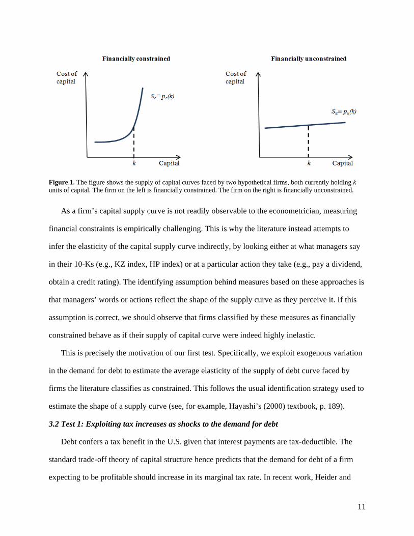
has been “cut out” of the capital markets. Figure 1 illustrates the definition graphically:

13 Fazzari, Hubbard, and Petersen (1988) note that when the supply curve becomes inelastic, “the cost of new debt and equity may differ substantially from the opportunity cost of internal finance generated through cash flow and retained earnings.”

11

Figure 1. The figure shows the supply of capital curves faced by two hypothetical firms, both currently holding k units of capital. The firm on the left is financially constrained. The firm on the right is financially unconstrained.

As a firm’s capital supply curve is not readily observable to the econometrician, measuring

financial constraints is empirically challenging. This is why the literature instead attempts to

infer the elasticity of the capital supply curve indirectly, by looking either at what managers say

in their 10-Ks (e.g., KZ index, HP index) or at a particular action they take (e.g., pay a dividend,

obtain a credit rating). The identifying assumption behind measures based on these approaches is

that managers’ words or actions reflect the shape of the supply curve as they perceive it. If this

assumption is correct, we should observe that firms classified by these measures as financially

constrained behave as if their supply of capital curve were indeed highly inelastic.

This is precisely the motivation of our first test. Specifically, we exploit exogenous variation

in the demand for debt to estimate the average elasticity of the supply of debt curve faced by

firms the literature classifies as constrained. This follows the usual identification strategy used to

estimate the shape of a supply curve (see, for example, Hayashi’s (2000) textbook, p. 189).

3.2 Test 1: Exploiting tax increases as shocks to the demand for debt

Debt confers a tax benefit in the U.S. given that interest payments are tax-deductible. The

standard trade-off theory of capital structure hence predicts that the demand for debt of a firm

expecting to be profitable should increase in its marginal tax rate. In recent work, Heider and

12

Ljungqvist (2013) provide evidence consistent with this prediction. Their identification strategy

exploits 43 staggered increases in state corporate income taxes in 24 U.S. states and 78 staggered

tax cuts in 27 states between 1989 and 2011. They find that, on average, public firms increase

their long-term leverage by 104 basis points in response to a tax increase measuring on average

131 basis points. Importantly, this is a pure capital-structure change: firms do not increase their

asset base overall, suggesting that investment opportunities remain unchanged and that the tax

shock increases their relative demand for debt but not their overall demand for capital. Heider

and Ljungqvist also show that firms do not reduce their leverage in response to tax cuts,

suggesting that the tax sensitivity of leverage is asymmetric.

Motivated by this evidence, we exploit increases (but not cuts) in state corporate income tax

rates as plausibly exogenous shocks to the demand for debt.14 This allows us to estimate the

shape of the debt supply curve faced by firms classified as either constrained or unconstrained.

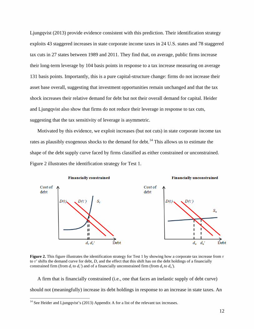
Figure 2 illustrates the identification strategy for Test 1.

Figure 2. This figure illustrates the identification strategy for Test 1 by showing how a corporate tax increase from τ to τ’ shifts the demand curve for debt, D, and the effect that this shift has on the debt holdings of a financially constrained firm (from dc to dc') and of a financially unconstrained firm (from du to du').

A firm that is financially constrained (i.e., one that faces an inelastic supply of debt curve)

should not (meaningfully) increase its debt holdings in response to an increase in state taxes. An

14 See Heider and Ljungqvist’s (2013) Appendix A for a list of the relevant tax increases.

13

unconstrained firm, on the other hand, should make full use of the additional tax shields by

issuing debt. Empirically, therefore, we can judge how well a financial constraints measure

actually captures constraints by testing for a higher average sensitivity of debt to tax increases

among firms classified as constrained than among firms classified as unconstrained.

In what follows, we discuss the identifying assumptions and limitations of Test 1, lay out the

empirical specifications we estimate, show that the test has power to identify financially

constrained firms, and test whether firms classified as financially constrained in the literature

respond less strongly to corporate tax increases than do firms classified as unconstrained.

3.2.1 Identifying assumptions and limitations

A key requirement for our identification strategy to be valid is that we can capture changes in

debt holdings that are the direct result of the tax increases and so are not confounded by other

shifts in the capital demand or supply curves. An important concern is that unobserved business

cycle factors cause both states to raise tax rates (shifting the demand for debt due to the increased

value of interest payments as tax shields) and, at the same time, firms to invest less (decreasing

their demand for capital) or banks to cut lending (shifting the supply of debt). For example, it is

possible that due to balanced-budget rules, states raise taxes when the local economy is weak

(and tax revenues fall) at the same time as banks suffer an increase in defaults and so cut lending.

Heider and Ljungqvist (2013) find no evidence that state tax changes correlate with observed

local business cycle effects, which is reassuring. To mitigate the potential influence of

unobserved business cycle effects, we follow their approach and exploit the local and staggered

nature of state tax increases. First, we estimate difference-in-differences tests, using as controls

firms that have not been affected by a tax increase. This establishes a counterfactual for the

observed change in debt holdings. Second, we restrict the control group to firms located in a state

adjacent to the tax-increase state. This differences away changes in debt holdings that are the

result of changes in local economic conditions and so allows us to identify the effect on debt

14

holdings of exogenous shifts in the debt demand curve induced by tax increases.15

Test 1 has two main limitations. First, given that tax shields are only of value to firms that

have (or expect soon to have) profits to shield from tax, the test cannot identify financial

constraints among chronically loss-making firms. To (conservatively) account for this, Test 1

excludes firm-years with losses. Second, Test 1 focuses on changes in the demand for debt, not

for equity. Thus, it can only identify whether firms classified as financially constrained are

unable to raise debt; it is silent regarding their ability to raise equity. Given that having restricted

access to the debt market is a necessary but not sufficient condition for a firm to be financially

constrained, the test allows us to effectively identify firms that are not financially constrained,

but it cannot unambiguously identify firms that are constrained.

3.2.2 Empirical specification

Equation (1) implements our empirical strategy for Test 1 as follows:

1 1ijst st it jt ijstD T X (1)

where i indexes firms, j industries, s headquarter states, and t fiscal years. The dependent

variable D is either long-term book leverage, as is common in the capital structure literature, or

log long-term debt. The latter allows us to show that our results are not driven by firms

increasing leverage through asset sales, without actually raising any debt. The main variable of

interest, T+, is a dummy variable equal to 1 if the state a firm is headquartered in increased its top

corporate income tax rate, and 0 otherwise.16,17 To ensure our results are not driven by changes

in debt holdings that are unrelated to the tax changes, the vector X includes controls for ROA,

15 Some corporate tax rises coincide with bank tax rises. This shifts the demand for debt out and the supply of debt in (see Test 2), biasing us against finding a significant response to corporate tax rises. Our estimates are thus conservative. More potentially problematic are corporate tax rises that coincide with bank tax cuts (as the increase in credit supply could allow even financially constrained firms to borrow more, undermining the identification strategy). Fortunately, bank tax cuts never coincide with corporate tax increases in our sample period. 16 Following Heider and Ljungqvist (2013), we lag this variable to ensure that firms have enough time to adjust their debt holdings in response to a corporate income tax increase. 17 Note that firms are taxed not where they are incorporated but where they operate (which Heider and Ljungqvist (2013) approximate using a firm’s headquarter state). We use Heider and Ljungqvist’s hand-collected HQ data, rather than Compustat’s (which suffers from backfill bias).

15

tangibility, firm size, and a proxy for investment opportunities. (For variable definitions and

details of their construction, see Appendix A.)

We estimate equation (1) using OLS in first-differences to remove time-invariant unobserved

firm heterogeneity and include industry-year fixed effects to remove the effects of unobserved

time-varying industry shocks. Following Heider and Ljungqvist (2013), the sample is restricted

to treated firms (those in a state experiencing a tax increase) using their immediate neighbors (in

all adjacent states that do not change tax rates) as controls. Constraining treated and control firms

to be neighbors minimizes the impact of unobserved differences in economic conditions between

treated and control firms.

3.2.3 Power

To see if Test 1 has enough power to identify constraints, we compare the average tax

sensitivity of debt among public firms in the U.S. to that of private U.S. firms contained in the

Sageworks database (see Asker, Farre-Mensa, and Ljungqvist (2013)).18 The assumption

motivating this power test is that private firms are more likely to be financially constrained than

public firms (see, for example, Saunders and Steffen (2011) for evidence consistent with this

assumption). Thus, if Test 1 has power to identify financial constraints, we should find that

private firms respond less strongly to tax increases than do public firms.

The results, reported in Table 2, support this prediction. To provide a baseline, column 1

shows that the average public firm increases its leverage by 1.1 percentage points in response to

a tax rise (p<0.001), compared to other firms operating in its industry located elsewhere in the

U.S. This is identical to the corresponding point estimate in Heider and Ljungqvist’s (2013)

Table 9. Column 2 restricts the control group to firm-years neighboring a tax-increase state. As

in Heider and Ljungqvist, requiring treated firms and their controls to be geographically

proximate increases the estimated tax sensitivity, to 1.3 percentage points (p<0.001). Columns 5

18 We restrict the sample of private firms to include only C Corps. Firms that are S Corps or are unincorporated pay personal rather than corporate income taxes and so are not affected by our corporate income tax shocks.

16

and 6 show that these results also hold when we use the change in log long-term debt as the

dependent variable: public firms significantly increase the amount of debt in their capital

structure, by between 8.6% and 10.1% on average. This alleviates concerns that our findings

might be driven by changes in firms’ total assets rather than in their debt holdings.

Overall, these results show that the average public firm is able to borrow more when its

demand for debt increases exogenously. This is not the case for private firms. Relative to private

control firms in neighboring states, private firms in treated states do not increase their leverage or

log debt outstanding significantly in response to a tax increase. In column 3, for example, the

point estimate is 0.4 percentage points with a p-value of 0.269 – less than a third of the average

public firm’s tax sensitivity. This is consistent with the assumption that private firms are more

likely to be financially constrained than public firms and so suggests that Test 1 has power to

identify financial constraints.

Columns 4 and 8 corroborate this conclusion by allowing private firms’ tax sensitivity to

differ depending on their size. While private firms in the three bottom size quartiles do not

increase their debt holdings significantly in response to a tax increase, the very largest private

firms do. Leverage, for example, increases by 1 percentage points among the largest firms

(p=0.021), not far off the point estimate for the average public firm. These patterns are consistent

with small private firms being more financially constrained than the very largest private firms,

which in turn behave more like public firms on average.

3.2.4 Are ‘constrained’ firms financially constrained?

Table 3 compares the tax sensitivity of debt holdings across firms classified as financially

constrained or unconstrained by the dividend and credit-rating measures, as well as by the KZ,

HP, and WW indices. Panels A and B show how long-term book leverage and log long-term

debt, respectively, respond to corporate tax increases.

The table reveals two noteworthy results. First, firms classified as constrained according to

17

each of the five measures are in fact able to increase their leverage significantly when their

demand for debt increases exogenously. So unlike (small) private firms, supposedly constrained

public firms can and do respond to tax increases. Second, there is no evidence that firms

classified as constrained react any less strongly than firms classified as unconstrained, whether

we focus on changes in leverage or in log debt.19

The results for Test 1 cast doubt on the ability of standard measures of financial constraints

to identify firms that are constrained in their ability to raise debt capital: none of the five

measures of financial constraints identifies firms with unusually inelastic supply of debt curves.

In fact, the estimated supply curves seem remarkably flat: the coefficients among ‘constrained’

firms range from 1.2 to 2.1 percentage-point increases in leverage. Economically, this implies

that the average ‘constrained’ firm raises new debt equivalent to between 19% and 38% of its

annual CAPEX spending (see Table 1) – a sizeable amount. The two caveats, as mentioned

before, are that Test 1 is silent on how constrained loss-making firms might be and that it cannot

speak to firms’ ability to raise equity when unable to raise debt. To address these caveats, we

introduce two alternative identification strategies.

3.3 Test 2: Exploiting bank tax changes as shocks to the supply of debt

Test 2 is based on the following premise. The behavior of an unconstrained firm should not

be affected by small shocks to capital supply that do not alter its investment opportunity set: if

one source of capital becomes, say, less plentiful, an unconstrained firm can simply substitute

towards another. A financially constrained firm, on the other hand, faces an inelastic capital

supply curve and thus should find itself less able to substitute across sources of capital.20 Its

19 Heider and Ljungqvist (2013) show that the leverage response to tax increases is smaller the more geographically dispersed a firm’s operations. The reason is that firms are taxed in each state in which they operate, so exposure to the tax treatment varies with the concentration of their operations in their HQ state. Table 1 shows that with the exception of the KZ index, ‘constrained’ firms have less dispersed operations, so we expect a larger tax sensitivity, all else equal. The data confirm this: in 7 of the 10 cases in Table 3, the estimated sensitivity is somewhat larger for ‘constrained’ firms, significantly so for the dividend measure (p-value for the difference in coefficients = 0.068). 20 This is similar in spirit to Lemmon and Roberts (2010), Chava and Purnanandam (2011), and Lin and Paravisini (2011), who analyze the effects of credit supply shocks on firm investment, performance, and risk, respectively.

18

reliance on debt should thus be more sensitive to shocks to the supply of debt from a particular

source. These predictions hold whether or not the firm is profitable, allowing us to address the

first limitation of Test 1.

To operationalize Test 2, we exploit 88 state-level changes in bank taxes between 1989 and

2011, listed in Appendix B. Importantly, for state tax purposes, states apportion a bank’s income

from lending to their state based on the location of the borrower, rather than the lender. Changes

in state bank taxes, by affecting the after-tax profitability of lending, thus directly affect the

supply of bank loans available to firms located in the state (though the economic magnitude of

the effect is an empirical question, which we address below). As a result, we expect banks to

expand lending in states with falling taxes and reduce it in states with rising taxes. Figure 3

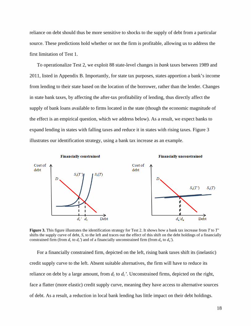
illustrates our identification strategy, using a bank tax increase as an example.

Figure 3. This figure illustrates the identification strategy for Test 2. It shows how a bank tax increase from T to T’ shifts the supply curve of debt, S, to the left and traces out the effect of this shift on the debt holdings of a financially constrained firm (from dc to dc') and of a financially unconstrained firm (from du to du').

For a financially constrained firm, depicted on the left, rising bank taxes shift its (inelastic)

credit supply curve to the left. Absent suitable alternatives, the firm will have to reduce its

reliance on debt by a large amount, from dc to dc’. Unconstrained firms, depicted on the right,

face a flatter (more elastic) credit supply curve, meaning they have access to alternative sources

of debt. As a result, a reduction in local bank lending has little impact on their debt holdings.

19

As in the previous section, we first discuss the identifying assumptions and limitations of the

test. We then show that bank tax changes affect bank lending, as required for identification, lay

out our empirical specifications, use the private-firm sample to show that the test has power to

identify financially constrained firms, and finally test if firms classified as constrained in the

literature are indeed sensitive to tax-induced variation in the local supply of bank loans.

3.3.1 Identifying assumptions and limitations

The key identifying assumption of Test 2 is that the tax-induced supply shocks are not

confounded by changes in firms’ demand for debt, allowing us to isolate changes in debt

holdings that are the direct result of changes in supply. This assumption faces two main potential

challenges: states don’t change bank taxes in a vacuum and bank tax changes could coincide

with the corporate tax changes we analyzed in Test 1. We address each concern in turn.

We follow a two-pronged approach to address the non-random nature of bank tax changes.

We first ask if observed variation in local conditions causes both states to change bank taxes and

firms to change their demand for debt. Table IA.1 in the Internet Appendix relates the probability

of a bank tax change to political and economic conditions, focusing on the governor’s political

affiliation, the state’s budget balance, bond rating changes, growth, unemployment, unionization,

and tax competition with neighboring states. This reveals that states are more likely to cut bank

taxes the larger their budget surplus, the higher their taxes relative to their neighbors, and if

governed by a Republican; and more likely to increase bank taxes the larger the budget deficit

and the lower their taxes relative to their neighbors. None of these factors has any obvious direct

link to firms’ demand for debt, mitigating omitted variable concerns. Second, as in Test 1, we

remove unobserved changes in local conditions by means of a diff-in-diff approach, using as

controls only firms headquartered in states that border a tax-change state.

When bank tax increases coincide with corporate tax increases, two things happen: credit

20

supply contracts and demand for credit increases.21 For a constrained firm, the demand increase

could partially offset the supply shock, leaving its debt holdings little changed. This would make

it look as if the firm were unaffected by the supply shock and hence unconstrained.22 Of the 88

bank tax changes in our sample, 24 are increases that coincided with a corporate tax rise. We

show in Table IA.2 in the Internet Appendix that our Test 2 results are robust to excluding these.

A more philosophical challenge when exploiting supply shocks to identify financial

constraints is how large the shock should ideally be. Too small and the test will have no power.

Too large and it will fundamentally change the shape of the capital supply curve for virtually all

firms. For instance, if the global financial system were to collapse due to another financial crisis,

a large number of previously unconstrained firms would presumably find themselves facing an

inelastic supply curve.23 But the aftermath of such a shock would not be particularly informative

of the financial constraints faced by such firms in more ordinary times. In other words, a large

shock to the financial system would have poor external validity.

In practice, changes in state bank taxes tend to be relatively small: over our sample period,

bank tax increases and cuts average 71 and –52 basis points, respectively. Tax shocks of these

magnitudes are unlikely to fundamentally alter the capital supply curves firms face. The greater

concern is instead whether the shocks are large enough to induce a significant change in lending

behavior.

The first three columns in Table 4 aim to answer this question. We use Call Report data from

the Federal Reserve to analyze the sensitivity of bank lending to changes in state bank taxes.

Specifically, we analyze how changes in a state’s bank tax rate affect (the logarithm of) the total

dollar amount of commercial and industrial (C&I) loans made by banks headquartered in that

21 We need not worry about the opposite case of bank tax cuts coinciding with corporate tax cuts, as Heider and Ljungqvist (2013) show that corporate tax cuts have no effect on firms’ demand for debt. 22 Contrast this with Test 1, where overlapping tax increases merely diminish the power of the test. 23 Graphically, a shock of such magnitude would not only shift the capital supply curve inward, as in Figure 3, but would make the capital supply curve of most previously unconstrained firms as inelastic as the Sc curve in Figure 1.

21

state,24 following a differences-in-differences approach similar to that used in Test 1. We find

that a one-percentage-point increase (cut) in state bank taxes is associated with a highly

significant 1.5 to 1.8 percent decrease (increase) in C&I loans made by banks headquartered in

the state, relative to untreated control banks in the adjacent states. This suggests that changes in

state bank taxes induce a significant change in bank lending behavior, a necessary requirement

for our identification strategy to be valid.

3.3.2 Empirical specification

Equation (2) captures our empirical strategy for Test 2, which as in Test 1 is estimated by

OLS in first-differences with the control group restricted to firms located in neighboring states to

those affected by a bank tax change:

1ijst st it jt ijstD BT X (2)

As before, i indexes firms, j industries, s firms’ headquarter states, and t fiscal years. In this case,

our main regressor of interest, BT, is a variable capturing the tax rate change (in percentage

points) affecting banks that lend in the state the firm is headquartered in (regardless of the banks’

own geographic location). As in Test 1, we model changes in both long-term book leverage and

log long-term debt, and we include the same control vector X as in equation (1). Unlike in the

case of Test 1, the identification strategy behind Test 2 does not require firms to be profitable

and so we include all firm-years in our analysis.

3.3.3 Power

To establish whether Test 2 has enough power to identify financial constraints, we compare

public and private firms’ sensitivity of debt holdings to changes in bank taxes, as an instrument

for changes in bank credit supply.25 To the extent that private firms, particularly small ones, are

more likely to face an inelastic debt supply curve, we expect their debt holdings to be more

24 We focus on banks with total assets between $500 million and $10 billion in 2005 dollars, thus excluding banks that are too small to provide any meaningful lending to public firms as well as the largest systemic banks that are too big to be affected by changes in individual states’ taxes. Excluding the largest banks has no impact on our results. 25 Unlike in Test 1, this test does not require the private-firm sample to be restricted to C Corps.

22

sensitive to shifts in the debt supply curve than those of public firms.

The results, shown in Table 4, are consistent with this prediction. In column 4, changes in

state bank taxes have no effect – either economically or statistically – on public firms’ leverage.

Private firms, on the other hand, respond significantly to shocks to bank credit supply. A one-

percentage-point increase (cut) in bank taxes in column 5 is associated with a 0.4 percentage

point reduction (increase) in leverage (p=0.004). Column 6 shows that this effect is driven by

smaller private firms, particularly those in the two smallest size quartiles; larger private firms

behave more like the average public firm in column 4. Columns 7 through 9 model log long-term

debt instead, with qualitatively similar, albeit somewhat noisier, results.

The results in Table 4 suggest that changes in a state’s bank taxes induce significant shifts in

the debt supply curve firms in that state face and that these changes can be exploited to identify

variation in financial constraints across firms.

3.3.4 Comparing the behavior of ‘constrained’ and ‘unconstrained’ firms

Table 5 reports the results of using Test 2 to examine if public firms classified as constrained

or unconstrained by the five financial constraints measures behave in a way that is consistent

with their classification. Specifically, we expect a negative effect of bank tax changes on the debt

holdings of financially constrained firms and no effect among financially unconstrained firms.

Panels A and B model long-term book leverage and log long-term debt, respectively.

Two results stand out. First, we find no evidence that supposedly constrained public firms

borrow less when bank taxes go up or borrow more when bank taxes fall. Thus, unlike the

private firms analyzed in Table 4 to establish the power of Test 2, the average public firm

classified as financially constrained does not behave in a way that suggests it actually is

financially constrained. Second, if anything, we find some evidence that supposedly

unconstrained firms behave in a constrained fashion: the debt holdings of ‘unconstrained’

dividend payers are at least marginally statistically more sensitive to bank tax changes than the

23

debt holdings of non-dividends payers; and the HP Index similarly appears to misclassify firms.

Overall, we find no evidence suggesting that the firms the literature would classify as

financially constrained react to shifts in their local debt supply curves. Taken together with our

findings in Test 1, these results cast doubt on the notion that these firms are in fact financially

constrained, in the sense of facing an inelastic supply of debt curve.

3.4 Test 3: Equity Recycling

Neither Test 1 nor Test 2 can identify firms that are constrained in the equity markets. Of

course, a firm that has access to the debt markets cannot meaningfully be called financially

constrained, whether or not it has easy access to the equity markets. In that sense, Tests 1 and 2

already suffice to show that existing measures of financial constraints do not correctly identify

firms that are financially constrained, as we have found their debt supply curves to be no steeper

than those of supposedly unconstrained firms.

Nevertheless, it would be useful to have a test that can identify equity constraints, so that

future researchers can evaluate other candidate financial constraints measures comprehensively:

to be classified as financially constrained, a firm would have to act as if it faced both an inelastic

debt supply curve and an inelastic equity supply curve. To this end, we propose a third test using

an alternative identification strategy to indirectly estimate the shape of the equity supply curve.

Test 3 is motivated by the findings of Farre-Mensa, Michaely, and Schmalz (2013), who

show that over the 1989-2012 period, 48.4% of the proceeds of public U.S. firms’ equity issues

were paid out again (via dividends or share repurchases) during the same year, a practice they

call “equity recycling.” The identifying assumption behind Test 3 is that we should not observe

equity recycling among firms facing an inelastic supply of equity curve:26 equity recycling, by

revealed preference, is an indicator that a firm is not concerned about its ability to raise equity

26 Farre-Mensa et al. explore reasons why firms may find it optimal to recycle equity. Whatever the reason, the only assumption for Test 3 to be valid is that equity recycling is suboptimal for a financially constrained firm.

24

and so is plausibly unconstrained.27

3.4.1 Empirical specification

Our analysis of what firms do with the proceeds of their equity issues adapts the framework

proposed by Kim and Weisbach (2008) to the empirical strategy of Tests 1 and 2. Specifically,

we use OLS in first-differences to estimate the following equation:

ijt ijt ijt ijt jt ijtP Equity Issue Other Sources of Funds Size (3)

where i indexes firms, j industries, and t fiscal years. The dependent variable, P for payout, can

be measured either as total payouts, adding up dividends and repurchases, or as dividends only.

The variable of interest, Equity Issue, captures a firm’s proceeds from SEOs, private stock

placements, stock option exercises, and employee stock ownership plans. Other Sources of

Funds captures operating cash flows, debt issues net of debt repurchases, and the proceeds from

asset sales. We also control for firm size and include industry-year fixed effects. All variables

(except for size) are scaled by beginning-of-year total assets.

3.4.2 Power

To establish power, we turn once more to our comparison of the behavior of public and

private firms. To the extent that private firms are more likely to face constraints in their ability to

raise equity, we expect them not to engage in equity recycling.

Table 6 confirms this prediction. Columns 1 and 2 show that for public firms, increases in

equity issuance proceeds are associated with highly significant increases in total payouts

(dividends plus repurchases, column 1) and in dividends (column 2). In other words, the average

public firm appears to “recycle equity,” suggesting it is not financially constrained. Column 3, on

the other hand, shows that private firms tend to cut their dividends at the same time they issue

equity.28 A plausible interpretation is that private firms use a combination of equity issues and

27 See Babenko, Lemmon, and Tserlukevich (2011) for a similar argument in the context of cash inflows from employee stock option exercises. 28 Sageworks does not report data on share repurchases, so we cannot analyze total payouts for private firms.

25

reductions in payouts to fund increases in their investment or operating needs. The point estimate

suggests that the average private firm reduces its dividend by 0.31 percentage points of total

assets for every 10 percentage-point increase in its equity-issuance-to-assets ratio. Column 4

shows that this effect is largest (in absolute value) for the smallest private firms and becomes

monotonically smaller (though remaining significant) for larger firms.

Absence of equity recycling is a necessary, but not a sufficient, condition for financial

constraints. Thus, the fact that private firms do not recycle equity does not imply that they are

necessarily financially constrained. The presence of equity recycling among public firms, on the

other hand, violates the necessary condition and so implies that public firms are not constrained

on average.

3.4.3 Comparing the behavior of ‘constrained’ and ‘unconstrained’ firms

Table 7 reports the results of examining whether or not firms the literature classifies as

financially constrained engage in equity recycling. For brevity, we focus on total payouts; results

are economically unchanged if we model dividends only instead.

Two results stand out. First, across all five constraints measures, we consistently find that

supposedly constrained firms do recycle their equity proceeds. Second, for only two of the five

measures do ‘constrained’ firms recycle less than ‘unconstrained’ firms: the dividend measure

and the KZ index. Unsurprisingly, dividend payers tend to distribute a significantly larger share

of their equity proceeds than non-dividend payers. Overall, firms classified as constrained by

each of the five measures engage in “equity recycling” behavior, which is hard to reconcile with

the notion that they are constrained in their ability to raise equity.

3.5 Validating The Methodological Approach: The Case of Junk Bond Issuers

The results of our three tests paint a consistent picture: the behavior of firms the literature

classifies as financially constrained does not appear to differ systematically from the behavior of

firms typically classified as unconstrained. In particular, the average ‘constrained’ firm (just like

26

the average ‘unconstrained’ one) is able to

borrow more when its demand for debt increases exogenously (Test 1);

maintain borrowing levels when banks lending in its home state are hit with a tax shock that

demonstrably affects their loan supply (Test 2); and

use a significant part of the proceeds of their equity issues to increase their payouts to

shareholders (Test 3).

In sharp contrast, none of our tests can rule out the hypothesis that private firms (particularly the

smaller ones) are indeed financially constrained. Taken together, these findings run counter to

the notion that firms commonly classified in the literature as financially constrained face an

inelastic supply of capital curve and so are indeed constrained.

As a final validation of our methodological approach, we apply our tests to a subsample of

public firms that are a priori likely to face inelastic capital supply curves and so are plausibly

financially constrained: junk bond issuers. Table 8 reports the results.

Columns 1 and 2 show that junk bond issuers fail Test 1: the tax sensitivity of debt among

junk bond issuers is not statistically different from zero, for either leverage or log debt. This is

consistent with junk bond issuers facing an inelastic debt supply curve on the margin.

Reinforcing this conclusion, columns 3 and 4 show that junk bond issuers reduce their debt

holdings significantly when bank lending in their home state is hit with a tax increase and vice

versa. This finding is consistent with the premise of Test 2 that the debt holdings of constrained

firms should be sensitive to shifts in their debt supply curve. Finally, unlike public firms in

general and those the literature traditionally classifies as constrained, junk bond issuers do not

engage in equity recycling. This is consistent with the premise of Test 3, as we should observe

no equity recycling among constrained firms.

The results in Table 8 help alleviate the concern that we fail to find support for traditional

measures of financial constraints simply because our tests lack the power to identify financial

27

constraints among any subsample of (public) firms. Indeed, the results suggest that public firms

with a below-investment grade credit rating face, on average, an inelastic supply of capital curve

and thus are financially constrained.

4. What do Traditional Measures of Financial Constraints Actually Measure?

The evidence presented in Section 3 suggests that firms classified as ‘constrained’ or

‘unconstrained’ by the five measures we examine do not actually differ, on average, in their

ability to raise debt or equity capital. Does this mean there are no meaningful differences

between these groups of firms? The fact that the empirical literature documents plenty of

differences in behavior suggests that tests based on these measures do pick up important

differences in firm types – just not, according to our tests, in financial constraints.29

The summary statistics and cross-tabulations in Table 1 suggest that public firms classified as

‘constrained’ by the dividends, ratings, HP, and WW measures look very different from

‘unconstrained’ firms (the KZ index is more of an outlier): ‘Constrained’ firms tend to be

younger, smaller, less profitable, and less leveraged than ‘unconstrained’ firms, but they also

grow faster and invest more, particularly in R&D. In this section, we investigate differences in

funding sources between ‘constrained’ and ‘unconstrained’ firms. As we will see, the five

measures produce sample splits that differ markedly in terms of funding patterns.

Table 9 shows the frequency with which ‘constrained’ and ‘unconstrained’ public firms issue

equity, sell bonds, or take out a loan. This reveals three important differences. First,

‘constrained’ firms are substantially more likely to fund themselves by issuing equity than are

‘unconstrained’ firms. For instance, 9.3% of non-dividend-payers raise equity from outside

investors in a given year, while only 4.3% of dividend-paying firms do so (a difference that is

significant at the 1% level). Firms classified as constrained by the KZ, HP, and WW indices

similarly raise equity more frequently than ‘unconstrained’ firms. (The only exceptions are non-

29 For instance, Giroud and Mueller (2013) show that ‘constrained’ firms (but not ‘unconstrained’ ones) reallocate capital and labor from less to more productive divisions.

28

rated and rated firms, which both raise equity with almost exactly the same frequency.)

Second, ‘constrained’ firms rely much less heavily on bond issues than ‘unconstrained’ firms

(except for the KZ index). For example, 21.3% of ‘unconstrained’ firms according to the HP

index issue bonds in a given year, whereas ‘constrained’ firms very rarely do so (1.3%).30 This

difference is mostly driven by issues of public bonds, which are rare among ‘constrained’ firms,

but it persists if we focus on bonds issued under rule 144A or placed privately.31

Third, while ‘constrained’ firms do not use the bond markets much, they do regularly access

the syndicated loan market: the fraction of ‘constrained’ firms obtaining a loan in a given year

ranges from 9.8% for the HP index to 27.6% for the dividends measure. This is consistent with

our finding in Test 1 that ‘constrained’ firms are able to borrow more when their demand for

debt increases due to exogenous increases in state corporate income taxes. Apparently, much of

this extra borrowing comes from loans rather than bonds.32

Taken together, the results in Tables 1 and 9 suggest that the five financial constraints

measures we examine do not generate a random partition of the universe of public firms. Rather

(with the exception of the KZ index), they tend to identify as ‘constrained’ firms that are

younger, smaller, and faster growing than ‘unconstrained’ firms. However, our three tests do not

support the hypothesis that these firms face inelastic supply curves of debt or equity capital, and

Table 9 confirms that these firms regularly access the public equity and bank-loan markets

(though not the bond market). A plausible reading of the evidence is that the dividends, ratings,

HP, and WW measures identify as ‘constrained’ public firms that find themselves in the growth

phase of their lifecycle. However, while these firms differ markedly from the more mature

‘unconstrained’ firms, they do not appear to be restricted in their ability to finance this growth, at

30 As in much of Table 1, the KZ index departs from this pattern: here, ‘constrained’ firms are more likely to issue bonds than ‘unconstrained’ firms (12.1% vs. 7.2%). 31 In particular, consistent with Faulkender and Petersen’s (2006) assumption that firms without a credit rating have no access to the public debt market, we find that a negligible 0.2% of unrated firms issue public debt in a given year. 32 This rules out the possibility that the lack of response to shocks to the local credit supply among ‘constrained’ firms in Test 2 reflects such firms not having access to bank loans in the first place.

29

least not during the average year in our sample period.

5. Conclusions

Much empirical research in corporate finance proxies for financial constraints using

measures that capture what firms say, do, or look like. We evaluate how well such measures

identify firms that are financially constrained, using three novel tests that help identify the

elasticity of a firm’s supply of capital curve: an exogenous increase in a firm’s demand for

credit; exogenous variation in the supply of bank loans; and the tendency for firms to pay out the

proceeds of equity issues to their shareholders (“equity recycling”).

We find that none of the five measures we evaluate is able to identify firms that behave as if

they were in fact constrained. Specifically, public firms classified as constrained for not paying

dividends or not having debt or according to the KZ, HP, or WW indices appear to have no

trouble raising debt when their demand for debt increases exogenously; are unaffected by

changes in the supply of bank loans; and engage in equity recycling. Furthermore, they differ

little in these respects from supposedly unconstrained firms, even though they are much smaller

and younger, grow considerably faster, and rarely access either the public or the private bond

market. But they appear to have ready access to both the equity markets and bank lending, which

appear to supply capital to them when they need it.

Our results imply that popular measures of financial constraints identify as constrained

subsets of firms that differ from the general firm population on a number of dimensions, but not

in their ability to raise external funding. This suggests that extant findings that have been

attributed to financial constraints are more likely to be caused by some other difference in firm

characteristics, such as size, age, growth rates, or preferred funding source.

While we have no reason to doubt that the firms Kaplan and Zingales (1997), Hadlock and

Pierce (2010), and Whited and Wu (2006) originally identify as constrained in their respective

samples truly were financially constrained, our results make us skeptical of the popular practice

30

to use the coefficients from these three studies to extrapolate to other samples and time periods in

an effort to identify potentially constrained firms. As regards the other two measures, we note

that paying a dividend or obtaining a credit rating are choices firms make endogenously and so

may be more reflective of the firm’s lifecycle than its ability to raise external funding.33

So which firms are financially constrained? Unfortunately, our methodological approach can

only be used to test whether a particular measure identifies firms that are plausibly financially

constrained – not to construct an alternative measure of financial constraints. The reason is that

our tests identify behavior that is necessary but not sufficient for a firm to be classified as

constrained. As a result, we cannot use the tests to unequivocally identify which firms are

financially constrained and which are not. Having said that, when applied to two groups of firms

that are plausibly financially constrained – small privately held firms and public firms with

below investment-grade ratings – our tests are able to identify behavior that is consistent with

our prior that these firms are indeed financially constrained.

33 For example, it is hard to believe that Microsoft was financially constrained before paying its first dividend in 2003 or that Apple was constrained before obtaining its first bond rating since 2004 in connection with its $17 billion bond issue in 2013, the largest corporate-bond deal in history.

31

References

Adam, Tim, 2009, Capital expenditures, financial constraints, and the use of options, Journal of Financial Economics 92, 238–251.

Almeida, Heitor, and Murillo Campello, 2001, Financial constraints and investment-cash flow sensitivities: New research directions, Unpublished working paper, New York University.

Almeida, Heitor, Murillo Campello, and Michael Weisbach, 2004, The cash flow sensitivity of cash, Journal of Finance 59, 1777–1804.

Almeida, Heitor, Murillo Campello, and Michael Weisbach, 2011, Corporate financial and investment policies when future financing is not frictionless, Journal of Corporate Finance 17, 675–693.

Almeida, Heitor, and Murillo Campello, 2010, Financing frictions and the substitution between internal and external funds, Journal of Financial and Quantitative Analysis 45, 589–622.

Asker, John, Joan Farre-Mensa, and Alexander Ljungqvist, 2013, Corporate investment and stock market listing: A puzzle?, Unpublished working paper, New York University.

Ball, Christopher, Gerard Hoberg, and Vojislav Maksimovic, 2012, Redefining financial constraints: A text-based analysis, Unpublished working paper, University of Maryland.

Babenko, Ilona, Michael Lemmon, and Yuri Tserlukevich, Employee stock options and investment, Journal of Finance 66, 981–1009.

Brockman, Paul, Xiumin Martin, and Emre Unlu, 2010, Executive compensation and the maturity structure of corporate debt, Journal of Finance 65, 1123–1161.

Chava, Sudheer, and Michael R. Roberts, 2008, How does financing impact investment? The role of debt covenants, Journal of Finance 63, 2085–2121.

Chava, Sudheer, and Amiyatosh Purnanandam, 2011, The effect of banking crisis on bank-dependent borrowers, Journal of Financial Economics 99, 116–135.

Denis, David J., and Valeriy Sibilkov, 2010, Financial constraints, investment, and the value of cash holdings, Review of Financial Studies 23, 247–269.

Duchin, Ran, Oguzhan Ozbas, and Berk A. Sensoy, 2010, Costly external finance, corporate investment, and the subprime mortgage credit crisis, Journal of Financial Economics 97, 418–435.

Farre-Mensa, Joan, Roni Michaely, and Martin Schmalz, 2013, Equity-recycled dividends, Work in progress.

Faulkender, Michael, and Mitchell A. Petersen, 2006, Does the source of capital affect capital structure?, Review of Financial Studies 19, 45–79.

Fazarri, Steven M., R. Glenn Hubbard, and Bruce C. Petersen, 1988, Financing constraints and corporate investment, Brookings Papers on Economic Activity.

Fazzari, Steven M., R. Glenn Hubbard, and Bruce C. Petersen, 2000, Investment-cash flow sensitivities are useful: A comment on Kaplan and Zingales, Quarterly Journal of Economics 115, 695–705.

Frank, Murray Z., and Vidhan K. Goyal, 2009, Capital structure decisions: Which factors are

32

reliably important?, Financial Management 38, 1–37.

Garcia, Diego, and Øyvind Norli, 2012, Geographic dispersion and stock returns, Journal of Financial Economics 106, 547–565.

Giroud, Xavier, and Holger Mueller, 2013, Capital and labor reallocation inside firms, Unpublished working paper, MIT.

Hadlock, Charles J., and Joshua R. Pierce, 2010, New evidence on measuring financial constraints: Moving beyond the KZ Index, Review of Financial Studies 23, 1909–1940.

Hayashi, Fumio, 1982, Tobin’s marginal q and average q: A neoclassical interpretation, Econometrica 50, 213–224.

Hayashi, Fumio, 2000, Econometrics, Princeton University Press.

Heider, Florian, and Alexander Ljungqvist, 2013, As certain as debt and taxes: Estimating the tax sensitivity of leverage from exogenous state tax changes, Unpublished working paper, New York University.

Hennessy, Christoper, and Toni Whited, 2007, How Costly is External Finance? Evidence from a Structural Estimation, Journal of Finance 62, 1705–1745.

Kaplan, Steven N., and Luigi Zingales, 1997, Do investment-cash flow sensitivities provide useful measures of financing constraints?, Quarterly Journal of Economics 115, 707–712.

Kashyap, Anil, Owen Lamont, and Jeremy Stein, 1994, Credit conditions and the cyclical behavior of inventories, Quarterly Journal of Economics 109, 565–592.

Kim, Woojin, and Michael S. Weisbach, 2008, Motivations for public equity offers: An international perspective, Journal of Financial Economics 87, 281–307.

Koch, Albin C., 2005, State taxation of banks and financial institutions (CA, IL, NY, TN), Tax Management Inc.

Lamont, Owen, Christopher Polk, and Jesus Saa-Requejo, 2001, Financial constraints and stock returns, Review of Financial Studies 14, 529–554.

Leary, Mark T., 2009, Bank loan supply, lender choice, and corporate capital structure, Journal of Finance 64, 1143–1185.

Lemmon, Michael, and Michael R. Roberts, 2010, The response of corporate financing and investment to changes in the supply of credit, Journal of Financial and Quantitative Analysis 45, 555–587.

Lin, Huidan, and Daniel Paravisini, 2011, The effect of financing constraints on risk, Review of Finance 17, 229–259.

Livdan, Dmitry, Haracio Sapriza, and Lu Zhang, 2009, Financially constrained stock returns, Journal of Finance 64, 1827–1862.

Rauh, Joshua D., 2006, Investment and financing constraints: Evidence from the funding of corporate pension plans, Journal of Finance 61, 33–71.

Rauh, Joshua D., and Amir Sufi, 2011, Capital structure and debt structure, Review of Financial Studies 23, 4242–4280.

Saunders, Anthony, and Sascha Steffen, 2011, The costs of being private: Evidence from the

33

loan market, Review of Financial Studies 24, 4091–4122.

Sufi, Amir, 2009, The real effects of debt certification: Evidence from the introduction of bank loan ratings, Review of Financial Studies 64, 1657–1695.

Tirole, Jean, 2006, The Theory of Corporate Finance, Princeton University Press.

Whited, Toni, 1992, Debt, liquidity constraints, and corporate investment: Evidence from panel data, Journal of Finance 47, 1425–1460.

Whited, Toni, and Guojun Wu, 2006, Financial constraints risk, Review of Financial Studies 19, 531–559.

34

Appendix A. Variable Definitions. Company-level variables Age is years since founding. We hand-collect founding dates from regulatory filings, business directories, and a comprehensive search of online and offline sources. Total real assets is defined as the book value of assets (Compustat item at) in year 2005 real dollars. Cash /assets is defined as Compustat items che/at. Tangibility is defined as net property, plant, and equipment (Compustat item ppent, or Sageworks NetFixedAssets), over total assets. ROA (return on assets) is defined as operating income before depreciation (Compustat item oibdp or its Sageworks equivalent, Sales – CostOfSales – Payroll – Rent – Advertising – Overhead + OtherOperatingIncome – OtherOperatingExpenses) over total assets. Profitable? is an indicator set equal to one if ROA is strictly positive, and zero otherwise. Total book leverage is defined as the sum of long-term debt (Compustat item dltt) and short-term debt (Compustat item dlc), over total assets. Book long-term leverage is defined as long-term debt (Compustat item dltt) over total assets (Compustat item at). For private firms, it is defined as Sageworks SeniorDebt + SubordinatedDebt over TotalAssets. % short-term debt (1 year) is defined as Compustat items dlc / (dlc + dltt). Any long-term debt? is an indicator set equal to one if Compustat item dltt is strictly positive, and zero otherwise. Investment opportunities is measured, for public firms, using a firm’s market to book ratio, constructed as in Frank and Goyal (2009). It is defined as (fiscal year-end closing price [prcc_f] times common shares used to calculate earnings per share [cshpri] + the liquidation value of preferred stock [pstkl] + long-term debt [dltt] + short-term debt [dlc] – deferred taxes and investment tax credits [txditc]) / total assets [at]. For private firms, we use the industry market to book ratio, estimated separately for each four-digit NAICS industry and each year. Sales growth is the annual percentage increase in sales: Salesit/Salesit-1 – 1 (using Compustat item sale). Employment growth is the annual percentage increase in employment: Employeesit/Employeesit-1 – 1 (using Compustat item emp). Gross investment is the annual increase in gross fixed assets (Compustat data item ppegt) scaled by beginning-of-year total assets. R&D is defined as Compustat item xrd over beginning-of-year total assets. Geographic concentration measures the geographic concentration in a firm’s operations and hence in its tax base across states. To capture where a firm operates, Garcia and Norli (2012) count the number of times a firm mentions each state it operates in in the Management Discussion and Analysis section of its 10-K filing. They then scale by the total number of mentions to obtain a proxy for the fraction of a firm’s operations that are associated with each state. We measure geographic concentration as the sum of the squared state-by-state fractions within firm and fiscal year (following the way the Herfindahl index is used to measure industry concentration). For example, a “single-state” firm has concentration of one, as all its operations are in a single state, while a firm whose operations are evenly distributed across all 50 states has concentration of 1/50. Log long-term debt is defined as the natural logarithm of one plus long-term debt (Compustat item dltt, or Sageworks SeniorDebt + SubordinatedDebt), deflated to 2005 dollars using the GDP deflator available at

35

http://www.bea.gov/national/xls/gdplev.xls. Fim size is defined as the natural logarithm of the book value of assets (Compustat item at, or Sageworks TotalAssets) in year 2005 real dollars. Dividends is defined as Compustat item dv for public firms and Sageworks item Dividends for private firms, scaled by beginning of year total assets. Dividends and repurchases is defined as the sum of Compustat items dv + prstkc, scaled by beginning of year total assets. Equity issuance proceeds is measured as Compustat item sstk for public firms and the change in Sageworks items TotalEquity – RetainedEarnings (set to 0 if negative) for private firms. Other sources of funds is defined, for public firms, as the sum of Compustat items dltis + ibc + dpc + sppe + siv, scaled by beginning of year total assets. For private firms, it is the sum of the change in long-term debt (Sageworks SeniorDebt + SubordinatedDebt, set to 0 if negative) + NetIncome + Depreciation + Amortization – change in GrossFixedAssets (set to 0 if negative), also scaled by beginning of year total assets. Log total assets is defined as the natural logarithm of beginning-of-year total assets (Compustat item at, or Sageworks TotalAssets) in year 2005 real dollars. Junk bond issuers are firms which in year t have a below investment-grade rating from S&P, Moody’s, or Fitch, using data obtained from Compustat (variable splticrm) and Mergent FISD. Financial constraints measures Non-dividend payers are firms with a history of zero dividends on common stock (Compustat item dvc), going as far back as 1970. Dividend payers are firms with a history of non-zero dividends on either common stock (Compustat item dvc), going as far back as 1970. Non-rated firms are those that do not have a credit rating from S&P, Moody’s, Fitch, or Duff & Phelps, using data obtained from Compustat (variable splticrm) and Mergent FISD. Rated firms are those that have a credit rating from S&P, Moody’s, Fitch, or Duff & Phelps, using data obtained from Compustat (variable splticrm) and Mergent FISD. KZ Index is constructed following Lamont, Polk, and Saa-Requejo (2001) as –1.001909[ (ib + dp)/lagged ppent] + 0.2826389[ (at + prcc_f×csho - ceq - txdb)/at] + 3.139193[(dltt + dlc)/(dltt + dlc + seq)] – 39.3678[(dvc + dvp)/lagged ppent] – 1.314759[che/lagged ppent], where all variables in italics are Compustat data items. Following convention, firms are sorted into terciles based on their index values in the previous year. Firms in the top tercile are coded as constrained and those in bottom tercile are coded as unconstrained. WW Index is constructed following Whited and Wu (2006) and Hennessy and Whited (2007) as –0.091 [(ib + dp)/at] – 0.062[indicator set to one if dvc + dvp is positive, and zero otherwise] + 0.021[dltt/at] – 0.044[log(at)] + 0.102[average industry sales growth, estimated separately for each three-digit SIC industry and each year, with sales growth defined as above] – 0.035[sales growth], where all variables in italics are Compustat data items. Following convention, firms are sorted into terciles based on their index values in the previous year. Firms in the top tercile are coded as constrained and those in bottom tercile are coded as unconstrained. HP Index is constructed following Hadlock and Pierce (2010) as –0.737Size + 0.043Size2 – 0.040Age, where Size equals the log of inflation-adjusted Compustat item at (in 2004 dollars), and Age is the number of years the firm is listed with a non-missing stock price on Compustat. In calculating the index, we follow Hadlock and Pierce and cap Size at (the log of) $4.5 billion and Age at 37 years. Following convention, firms are sorted into terciles based on

36

their index values in the previous year. Firms in the top tercile are coded as constrained and those in bottom tercile are coded as unconstrained. Bank-level variables Log commercial and industrial loans is defined as the natural logarithm of one plus rcon1766 from the Federal Reserve’s bank call reports, deflated to 2005 dollars using the GDP deflator. Call report data for 1976 to 2010 are available at http://www.chicagofed.org/webpages/banking/financial_institution_reports/commercial_bank_data.cfm. Data for 2011 and beyond are available at https://cdr.ffiec.gov/public/. We filter out banks involved in a merger and foreign filers. (We thank Kristy Agostino from the Chicago Fed for providing us with the merger data.) To annualize the quarterly Call report data, we focus on observations from the fourth quarter. Log deposits is defined as the natural logarithm of one plus rcon2200 from the Federal Reserve’s bank call reports, deflated to 2005 dollars using the GDP deflator. Log total assets is defined as the natural logarithm of one plus rcon2170 from the Federal Reserve’s bank call reports, deflated to 2005 dollars using the GDP deflator. State-level variables Corporate income tax increase is an indicator set equal to one if the state increased its corporate income tax rate, and zero otherwise. In states with more than one tax bracket, we focus on changes to the top bracket. See Appendix A in Heider and Ljungqvist (2013) for a complete list corporate income tax increases. Bank tax change equals the change (in percentage points) in the state income tax rate affecting banks and other financial institutions operating in the state. See Appendix B for a complete list of state bank tax increases and cuts, respectively. Democratic governor is an indicator set equal to one if the state is governed by a Democratic governor, and zero otherwise. Data come from the Congressional Quarterly (through 2008) and state election websites (after 2008). State budget balance equals the difference between a state’s general revenues and its general expenditures scaled by its general expenditures. The data come from the U.S. Census Bureau’s State & Local Finances database, available at http://www.census.gov/govs/local. State budget deficit equals state budget balance if the state runs a budget deficit, and zero otherwise. State budget surplus equals state budget balance if the state runs a budget surplus, and zero otherwise. State bond rating downgrade is an indicator set equal to one if the state’s credit rating is downgraded by either S&P or Moody’s. GSP growth rate is the real annual growth rate in gross state product (GSP) using data obtained from the U.S. Bureau of Economic Analysis. State unemployment rate is the state unemployment rate, obtained from the U.S. Bureau of Labor Statistics. State union penetration is the fraction of private-sector employees in a state who belong to a labor union in year t. The data come from Hirsch and Macpherson (2003) as updated on their website, http://www.unionstats.com. Tax competition is measured as the difference between a state’s corporate income tax rate and the highest corporate income tax rate levied by any of the neighboring states.

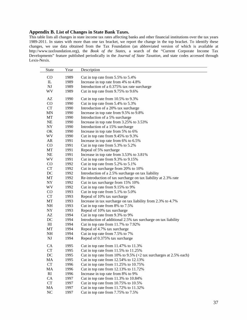
37

Appendix B. List of Changes in State Bank Taxes. This table lists all changes in state income tax rates affecting banks and other financial institutions over the tax years 1989-2011. In states with more than one tax bracket, we report the change in the top bracket. To identify these changes, we use data obtained from the Tax Foundation (an abbreviated version of which is available at http://www.taxfoundation.org), the Book of the States, a search of the “Current Corporate Income Tax Developments” feature published periodically in the Journal of State Taxation, and state codes accessed through Lexis-Nexis.

State Year Description

CO 1989 Cut in top rate from 5.5% to 5.4% IL 1989 Increase in top rate from 4% to 4.8% NJ 1989 Introduction of a 0.375% tax rate surcharge

WV 1989 Cut in top rate from 9.75% to 9.6%

AZ 1990 Cut in top rate from 10.5% to 9.3% CO 1990 Cut in top rate from 5.4% to 5.3% CT 1990 Introduction of a 20% tax surcharge MN 1990 Increase in top rate from 9.5% to 9.8% MT 1990 Introduction of a 5% surcharge NE 1990 Increase in top rate from 3.25% to 3.53% NY 1990 Introduction of a 15% surcharge OK 1990 Increase in top rate from 5% to 6% WV 1990 Cut in top rate from 9.45% to 9.3% AR 1991 Increase in top rate from 6% to 6.5% CO 1991 Cut in top rate from 5.3% to 5.2% MT 1991 Repeal of 5% surcharge NE 1991 Increase in top rate from 3.53% to 3.81% WV 1991 Cut in top rate from 9.3% to 9.15% CO 1992 Cut in top rate from 5.2% to 5.1% CT 1992 Cut in tax surcharge from 20% to 10% DC 1992 Introduction of a 2.5% surcharge on tax liability MT 1992 Re-introduction of tax surcharge on tax liability at 2.3% rate NY 1992 Cut in tax surcharge from 15% 10% WV 1992 Cut in top rate from 9.15% to 9% CO 1993 Cut in top rate from 5.1% to 5.0% CT 1993 Repeal of 10% tax surcharge MT 1993 Increase in tax surcharge on tax liability from 2.3% to 4.7% NH 1993 Cut in top rate from 8% to 7.5% NY 1993 Repeal of 10% tax surcharge AZ 1994 Cut in top rate from 9.3% to 9% DC 1994 Introduction of additional 2.5% tax surcharge on tax liability HI 1994 Cut in top rate from 11.7% to 7.92% MT 1994 Repeal of 4.7% tax surcharge NH 1994 Cut in top rate from 7.5% to 7% NJ 1994 Repeal of 0.375% tax surcharge

CA 1995 Cut in top rate from 11.47% to 11.3% CT 1995 Cut in top rate from 11.5% to 11.25% DC 1995 Cut in top rate from 10% to 9.5% (+2 tax surcharges at 2.5% each) MA 1995 Cut in top rate from 12.54% to 12.13% CT 1996 Cut in top rate from 11.25% to 10.75% MA 1996 Cut in top rate from 12.13% to 11.72% RI 1996 Increase in top rate from 8% to 9% CA 1997 Cut in top rate from 11.3% to 10.84% CT 1997 Cut in top rate from 10.75% to 10.5% MA 1997 Cut in top rate from 11.72% to 11.32% NC 1997 Cut in top rate from 7.75% to 7.5%

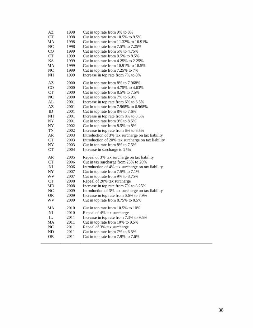
38

AZ 1998 Cut in top rate from 9% to 8% CT 1998 Cut in top rate from 10.5% to 9.5% MA 1998 Cut in top rate from 11.32% to 10.91% NC 1998 Cut in top rate from 7.5% to 7.25% CO 1999 Cut in top rate from 5% to 4.75% CT 1999 Cut in top rate from 9.5% to 8.5% KS 1999 Cut in top rate from 4.25% to 2.25% MA 1999 Cut in top rate from 10.91% to 10.5% NC 1999 Cut in top rate from 7.25% to 7% NH 1999 Increase in top rate from 7% to 8%

AZ 2000 Cut in top rate from 8% to 7.968% CO 2000 Cut in top rate from 4.75% to 4.63% CT 2000 Cut in top rate from 8.5% to 7.5% NC 2000 Cut in top rate from 7% to 6.9% AL 2001 Increase in top rate from 6% to 6.5% AZ 2001 Cut in top rate from 7.968% to 6.968% ID 2001 Cut in top rate from 8% to 7.6% NH 2001 Increase in top rate from 8% to 8.5% NY 2001 Cut in top rate from 9% to 8.5% NY 2002 Cut in top rate from 8.5% to 8% TN 2002 Increase in top rate from 6% to 6.5% AR 2003 Introduction of 3% tax surcharge on tax liability CT 2003 Introduction of 20% tax surcharge on tax liability NY 2003 Cut in top rate from 8% to 7.5% CT 2004 Increase in surcharge to 25%

AR 2005 Repeal of 3% tax surcharge on tax liability CT 2006 Cut in tax surcharge from 25% to 20% NJ 2006 Introduction of 4% tax surcharge on tax liability NY 2007 Cut in top rate from 7.5% to 7.1% WV 2007 Cut in top rate from 9% to 8.75% CT 2008 Repeal of 20% tax surcharge MD 2008 Increase in top rate from 7% to 8.25% NC 2009 Introduction of 3% tax surcharge on tax liability OR 2009 Increase in top rate from 6.6% to 7.9% WV 2009 Cut in top rate from 8.75% to 8.5%

MA 2010 Cut in top rate from 10.5% to 10% NJ 2010 Repeal of 4% tax surcharge IL 2011 Increase in top rate from 7.3% to 9.5%

MA 2011 Cut in top rate from 10% to 9.5% NC 2011 Repeal of 3% tax surcharge ND 2011 Cut in top rate from 7% to 6.5% OR 2011 Cut in top rate from 7.9% to 7.6%

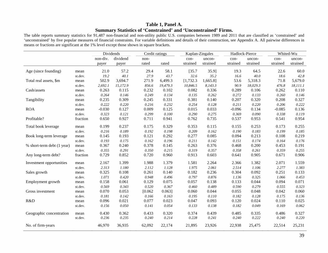
39

Table 1, Panel A. Summary Statistics of ‘Constrained’ and ‘Unconstrained’ Firms.

The table reports summary statistics for 91,487 non-financial and non-utility public U.S. companies between 1989 and 2011 that are classified as ‘constrained’ and ‘unconstrained’ by five popular measures of financial constraints. For variable definitions and details of their construction, see Appendix A. All pairwise differences in means or fractions are significant at the 1% level except those shown in square brackets.

Dividends Credit ratings Kaplan-Zingales Hadlock-Pierce Whited-Wu

non-div.

payer dividend

payer non-rated rated

con-strained

uncon-strained

con-strained

uncon-strained

con-strained

uncon-strained

Age (since founding) mean 21.0 57.2 29.4 58.1 [35.7 35.9] 19.3 64.5 22.6 60.0 st.dev. 19.2 40.1 27.9 43.7 32.6 35.2 16.6 40.0 18.6 42.8 Total real assets, $m mean 502.9 3,694.7 271.9 6,499.3 [1,732.3 1,665.8] 53.6 5,318.3 71.8 5,679.0 st.dev. 2,692.1 15,172.9 856.6 19,479.3 10,846.5 8,143.3 90.9 18,029.3 476.8 18,111.1 Cash/assets mean 0.263 0.115 0.232 0.102 0.082 0.336 0.289 0.106 0.262 0.110 st.dev. 0.264 0.146 0.249 0.134 0.135 0.262 0.272 0.133 0.260 0.146 Tangibility mean 0.235 0.309 0.245 0.331 0.381 0.140 0.207 0.320 0.208 0.327 st.dev. 0.222 0.220 0.216 0.232 0.254 0.128 0.211 0.220 0.206 0.222 ROA mean -0.030 0.127 0.009 0.125 0.015 0.033 -0.096 0.134 -0.085 0.136 st.dev. 0.323 0.121 0.299 0.100 0.290 0.275 0.369 0.090 0.338 0.119 Profitable? fraction 0.650 0.927 0.711 0.941 0.762 0.735 0.537 0.953 0.541 0.954

Total book leverage mean 0.199 0.237 0.175 0.329 0.353 0.115 0.155 0.253 0.173 0.255 st.dev. 0.216 0.189 0.192 0.198 0.209 0.162 0.190 0.183 0.199 0.185 Book long-term leverage mean 0.145 0.193 0.121 0.292 0.277 0.085 0.094 0.213 0.108 0.219 st.dev. 0.193 0.175 0.162 0.196 0.211 0.142 0.151 0.174 0.164 0.176 % short-term debt (1 year) mean 0.367 0.240 0.378 0.145 0.263 0.376 0.468 0.200 0.453 0.191 st.dev. 0.355 0.291 0.350 0.215 0.319 0.357 0.358 0.261 0.359 0.255 Any long-term debt? fraction 0.729 0.852 0.720 0.960 0.913 0.603 0.641 0.905 0.671 0.906

Investment opportunities mean 2.167 1.399 1.988 1.379 1.581 2.264 2.366 1.382 2.071 1.559 st.dev. 2.313 1.180 2.112 1.128 1.975 2.061 2.514 1.106 2.277 1.383 Sales growth mean 0.325 0.108 0.261 0.140 0.182 0.236 0.304 0.092 0.251 0.133 st.dev. 1.071 0.420 0.948 0.496 0.797 0.876 1.136 0.325 1.066 0.453 Employment growth mean 0.158 0.061 0.129 0.075 0.057 0.138 0.133 0.044 0.094 0.071 st.dev. 0.569 0.343 0.520 0.367 0.460 0.489 0.590 0.279 0.555 0.323 Gross investment mean 0.070 0.053 [0.062 0.063] 0.060 0.044 0.055 0.048 0.042 0.060 st.dev. 0.181 0.142 0.166 0.163 0.195 0.110 0.182 0.128 0.175 0.136 R&D mean 0.096 0.021 0.077 0.023 0.047 0.093 0.120 0.024 0.110 0.025 st.dev. 0.156 0.050 0.141 0.054 0.133 0.138 0.182 0.049 0.169 0.062

Geographic concentration mean 0.430 0.362 0.433 0.320 0.374 0.439 0.485 0.335 0.486 0.327 st.dev. 0.236 0.235 0.240 0.214 0.228 0.241 0.240 0.222 0.240 0.220

No. of firm-years 46,970 36,935 62,092 22,174 21,895 23,926 22,938 25,475 22,514 25,231

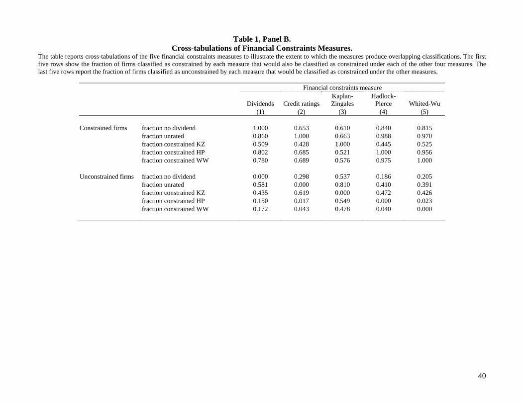
40

Table 1, Panel B. Cross-tabulations of Financial Constraints Measures.

The table reports cross-tabulations of the five financial constraints measures to illustrate the extent to which the measures produce overlapping classifications. The first five rows show the fraction of firms classified as constrained by each measure that would also be classified as constrained under each of the other four measures. The last five rows report the fraction of firms classified as unconstrained by each measure that would be classified as constrained under the other measures.

Financial constraints measure

Dividends Credit ratings Kaplan-Zingales

Hadlock-Pierce Whited-Wu

(1) (2) (3) (4) (5) Constrained firms fraction no dividend 1.000 0.653 0.610 0.840 0.815 fraction unrated 0.860 1.000 0.663 0.988 0.970 fraction constrained KZ 0.509 0.428 1.000 0.445 0.525 fraction constrained HP 0.802 0.685 0.521 1.000 0.956 fraction constrained WW 0.780 0.689 0.576 0.975 1.000 Unconstrained firms fraction no dividend 0.000 0.298 0.537 0.186 0.205 fraction unrated 0.581 0.000 0.810 0.410 0.391 fraction constrained KZ 0.435 0.619 0.000 0.472 0.426 fraction constrained HP 0.150 0.017 0.549 0.000 0.023 fraction constrained WW 0.172 0.043 0.478 0.040 0.000

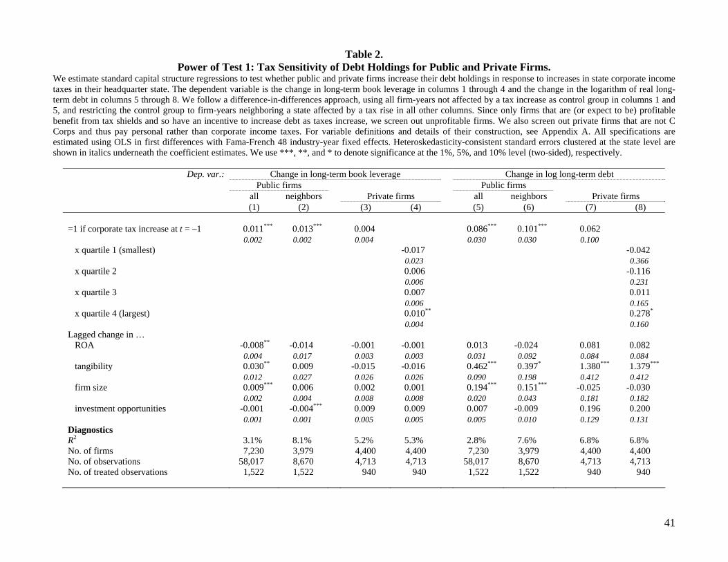
41

Table 2. Power of Test 1: Tax Sensitivity of Debt Holdings for Public and Private Firms.

We estimate standard capital structure regressions to test whether public and private firms increase their debt holdings in response to increases in state corporate income taxes in their headquarter state. The dependent variable is the change in long-term book leverage in columns 1 through 4 and the change in the logarithm of real long-term debt in columns 5 through 8. We follow a difference-in-differences approach, using all firm-years not affected by a tax increase as control group in columns 1 and 5, and restricting the control group to firm-years neighboring a state affected by a tax rise in all other columns. Since only firms that are (or expect to be) profitable benefit from tax shields and so have an incentive to increase debt as taxes increase, we screen out unprofitable firms. We also screen out private firms that are not C Corps and thus pay personal rather than corporate income taxes. For variable definitions and details of their construction, see Appendix A. All specifications are estimated using OLS in first differences with Fama-French 48 industry-year fixed effects. Heteroskedasticity-consistent standard errors clustered at the state level are shown in italics underneath the coefficient estimates. We use ***, **, and * to denote significance at the 1%, 5%, and 10% level (two-sided), respectively.

Dep. var.: Change in long-term book leverage Change in log long-term debt Public firms Public firms all neighbors Private firms all neighbors Private firms (1) (2) (3) (4) (5) (6) (7) (8) =1 if corporate tax increase at t = –1 0.011*** 0.013*** 0.004 0.086*** 0.101*** 0.062 0.002 0.002 0.004 0.030 0.030 0.100 x quartile 1 (smallest) -0.017 -0.042 0.023 0.366 x quartile 2 0.006 -0.116 0.006 0.231 x quartile 3 0.007 0.011 0.006 0.165 x quartile 4 (largest) 0.010** 0.278* 0.004 0.160 Lagged change in … ROA -0.008** -0.014 -0.001 -0.001 0.013 -0.024 0.081 0.082 0.004 0.017 0.003 0.003 0.031 0.092 0.084 0.084 tangibility 0.030** 0.009 -0.015 -0.016 0.462*** 0.397* 1.380*** 1.379*** 0.012 0.027 0.026 0.026 0.090 0.198 0.412 0.412 firm size 0.009*** 0.006 0.002 0.001 0.194*** 0.151*** -0.025 -0.030 0.002 0.004 0.008 0.008 0.020 0.043 0.181 0.182 investment opportunities -0.001 -0.004*** 0.009 0.009 0.007 -0.009 0.196 0.200 0.001 0.001 0.005 0.005 0.005 0.010 0.129 0.131 Diagnostics R2 3.1% 8.1% 5.2% 5.3% 2.8% 7.6% 6.8% 6.8% No. of firms 7,230 3,979 4,400 4,400 7,230 3,979 4,400 4,400 No. of observations 58,017 8,670 4,713 4,713 58,017 8,670 4,713 4,713 No. of treated observations 1,522 1,522 940 940 1,522 1,522 940 940

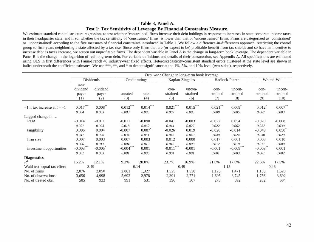
42

Table 3, Panel A. Test 1: Tax Sensitivity of Leverage By Financial Constraints Measure.

We estimate standard capital structure regressions to test whether ‘constrained’ firms increase their debt holdings in response to increases in state corporate income taxes in their headquarter state, and if so, whether the tax sensitivity of ‘constrained’ firms’ is lower than that of ‘unconstrained’ firms. Firms are categorized as ‘constrained’ or ‘unconstrained’ according to the five measures of financial constraints introduced in Table 1. We follow a difference-in-differences approach, restricting the control group to firm-years neighboring a state affected by a tax rise. Since only firms that are (or expect to be) profitable benefit from tax shields and so have an incentive to increase debt as taxes increase, we screen out unprofitable firms. The dependent variable in Panel A is the change in long-term book leverage. The dependent variable in Panel B is the change in the logarithm of real long-term debt. For variable definitions and details of their construction, see Appendix A. All specifications are estimated using OLS in first differences with Fama-French 48 industry-year fixed effects. Heteroskedasticity-consistent standard errors clustered at the state level are shown in italics underneath the coefficient estimates. We use ***, **, and * to denote significance at the 1%, 5%, and 10% level (two-sided), respectively. Dep. var.: Change in long-term book leverage Dividends Credit ratings Kaplan-Zingales Hadlock-Pierce Whited-Wu

non-dividend

payer dividend

payer unrated rated con-

strained uncon-strained

con-strained

uncon-strained

con-strained

uncon-strained

(1) (2) (3) (4) (5) (6) (7) (8) (9) (10) =1 if tax increase at t = –1 0.017*** 0.008** 0.012*** 0.014*** 0.021*** 0.015*** 0.021** 0.009* 0.012* 0.007** 0.004 0.003 0.003 0.005 0.007 0.005 0.008 0.005 0.007 0.003 Lagged change in … ROA -0.014 -0.011 -0.011 -0.090 -0.041 -0.003 -0.027 0.054 -0.020 -0.008 0.021 0.023 0.018 0.062 0.044 0.027 0.022 0.062 0.027 0.030 tangibility 0.006 0.004 -0.007 0.087* -0.026 0.019 -0.020 -0.014 -0.049 0.050* 0.041 0.026 0.034 0.051 0.045 0.040 0.040 0.024 0.030 0.029 firm size 0.007 0.003 0.007 0.003 0.012 0.000 0.017 0.001 0.003 0.010 0.006 0.011 0.004 0.013 0.013 0.008 0.012 0.010 0.011 0.009 investment opportunities -0.003*** -0.005* -0.004*** 0.001 -0.011*** -0.001 -0.001 -0.009*** -0.003** 0.001 0.001 0.003 0.001 0.006 0.004 0.001 0.001 0.003 0.001 0.002 Diagnostics R2 15.2% 12.1% 9.3% 20.0% 23.7% 16.9% 21.6% 17.6% 22.6% 17.5% Wald test: equal tax effect 3.49* 0.14 0.49 1.15 0.46 No. of firms 2,076 2,050 2,861 1,327 1,525 1,538 1,125 1,471 1,153 1,620 No. of observations 3,656 4,998 5,692 2,978 2,391 2,771 1,695 3,745 1,756 3,692 No. of treated obs. 585 933 991 531 396 507 273 692 282 684

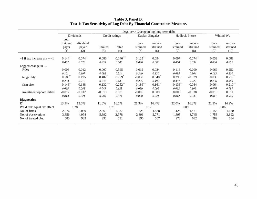
43

Table 3, Panel B. Test 1: Tax Sensitivity of Log Debt By Financial Constraints Measure.

Dep. var.: Change in log long-term debt Dividends Credit ratings Kaplan-Zingales Hadlock-Pierce Whited-Wu

non-dividend

payer dividend

payer unrated rated con-

strained uncon-strained

con-strained

uncon-strained

con-strained

uncon-strained

(1) (2) (3) (4) (5) (6) (7) (8) (9) (10) =1 if tax increase at t = –1 0.144** 0.074** 0.080** 0.146*** 0.125*** 0.094 0.097 0.074** 0.033 0.083 0.062 0.028 0.035 0.045 0.036 0.060 0.068 0.032 0.036 0.052 Lagged change in … ROA -0.008 -0.012 0.007 -0.595 0.012 0.024 -0.118 0.200 -0.069 0.252 0.101 0.197 0.092 0.514 0.249 0.120 0.095 0.364 0.113 0.200 tangibility 0.580** 0.195 0.402* 0.759* -0.030 0.848* 0.398 -0.029 0.033 0.719* 0.283 0.215 0.232 0.443 0.265 0.492 0.307 0.223 0.236 0.369 firm size 0.148** 0.148 0.132*** 0.252** 0.186*** 0.161* 0.138** -0.084 0.064 0.210** 0.065 0.088 0.043 0.123 0.059 0.096 0.062 0.106 0.076 0.097 investment opportunities -0.012 -0.012 -0.013 0.081 -0.005 0.009 0.003 -0.038 -0.010 0.011 0.013 0.021 0.008 0.074 0.028 0.021 0.012 0.036 0.011 0.046 Diagnostics R2 13.5% 12.0% 11.6% 16.1% 21.3% 16.4% 22.0% 16.3% 21.3% 14.2% Wald test: equal tax effect 1.28 1.71 0.17 0.09 0.86 No. of firms 2,076 2,050 2,861 1,327 1,525 1,538 1,125 1,471 1,153 1,620 No. of observations 3,656 4,998 5,692 2,978 2,391 2,771 1,695 3,745 1,756 3,692 No. of treated obs. 585 933 991 531 396 507 273 692 282 684

44

Table 4. Power of Test 2: Tax Sensitivity of Banks’ Loan Supply and of Public and Private Firms’ Debt Holdings.

The first three columns use Call Report data from the Federal Reserve to test whether increases (cuts) in state bank taxes induce a decrease (increase) in commercial and industrial lending by banks headquartered in the affected state. Columns 4 through 9 report standard capital structure regressions to test whether public and private firms decrease (increase) their debt holdings in response to an inward (outward) shift in the supply of credit induced by an increase (cut) in state bank taxes in their headquarter state. In all columns, we follow a difference-in-differences approach, restricting the control group to observations neighboring a state affected by a tax change. For variable definitions and details of their construction, see Appendix A. All specifications are estimated using OLS in first differences with year fixed effects in columns 1-3 and Fama-French 48 industry-year fixed effects in columns 4-9. Heteroskedasticity-consistent standard errors clustered at the state level are shown in italics underneath the coefficient estimates. We use ***, **, and * to denote significance at the 1%, 5%, and 10% level (two-sided), respectively.

Dep. var.: Change in log commercial Change in long-term book leverage Change in log long-term debt and industrial loans Public Private firms Public Private firms (1) (2) (3) (4) (5) (6) (7) (8) (9)

Bank tax change (in %) at t = 0 -0.018*** -0.018*** -0.015*** -0.001 -0.004*** -0.020 -0.003 0.006 0.005 0.005 0.001 0.001 0.013 0.004 x quartile 1 (smallest) -0.005* -0.006* 0.002 0.004 x quartile 2 -0.006*** -0.009*** 0.002 0.003 x quartile 3 -0.004 -0.008 0.003 0.007 x quartile 4 (largest) -0.002 0.011 0.002 0.015 Lagged change in … ROA -0.006 0.001 0.001 -0.019 0.001 0.001 0.274 0.001 0.001 0.550 0.007 0.007 tangibility 0.038** -0.027 -0.027 0.351*** -0.004 -0.004 0.027 0.017 0.017 0.005 0.033 0.033 firm size 0.007*** 0.004 0.004 0.160*** 0.022* 0.022* 0.002 0.004 0.004 0.000 0.012 0.012 investment opportunities 0.000 -0.001 -0.001 0.013*** -0.010 -0.010 0.413 0.002 0.002 0.000 0.010 0.010 log deposits 0.315*** 0.058 log total assets 0.575*** 0.045 Diagnostics R2 7.3% 9.7% 12.1% 4.1% 2.3% 2.3% 4.1% 2.4% 2.4% F test: bank tax change = 0 10.0*** 14.5*** 7.8*** n.a. n.a. n.a. n.a. n.a. n.a. No. of banks/firms 1,612 1,612 1,612 6,824 13,355 13,355 6,824 13,355 13,355 No. of observations 5,100 5,100 5,100 27,743 19,654 19,654 27,743 19,654 19,654 No. of treated obs. 1,289 1,289 1,289 8,339 3,591 3,591 8,339 3,591 3,591

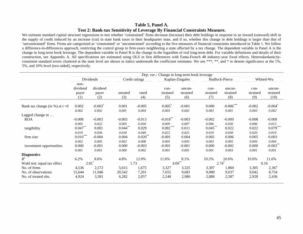
45

Table 5, Panel A. Test 2: Bank-tax Sensitivity of Leverage By Financial Constraints Measure.

We estimate standard capital structure regressions to test whether ‘constrained’ firms decrease (increase) their debt holdings in response to an inward (outward) shift in the supply of credit induced by an increase (cut) in state bank taxes in their headquarter state, and if so, whether this change in debt holdings is larger than that of ‘unconstrained’ firms. Firms are categorized as ‘constrained’ or ‘unconstrained’ according to the five measures of financial constraints introduced in Table 1. We follow a difference-in-differences approach, restricting the control group to firm-years neighboring a state affected by a tax change. The dependent variable in Panel A is the change in long-term book leverage. The dependent variable in Panel B is the change in the logarithm of real long-term debt. For variable definitions and details of their construction, see Appendix A. All specifications are estimated using OLS in first differences with Fama-French 48 industry-year fixed effects. Heteroskedasticity-consistent standard errors clustered at the state level are shown in italics underneath the coefficient estimates. We use ***, **, and * to denote significance at the 1%, 5%, and 10% level (two-sided), respectively. Dep. var.: Change in long-term book leverage Dividends Credit ratings Kaplan-Zingales Hadlock-Pierce Whited-Wu

non-dividend

payer dividend

payer unrated rated con-

strained uncon-strained

con-strained

uncon-strained

con-strained

uncon-strained

(1) (2) (3) (4) (5) (6) (7) (8) (9) (10) Bank tax change (in %) at t =0 0.002 -0.003* 0.001 -0.005 0.005* -0.001 0.000 -0.006*** -0.002 -0.004* 0.002 0.002 0.001 0.004 0.003 0.002 0.003 0.001 0.003 0.002 Lagged change in … ROA -0.008 -0.003 -0.003 -0.013 -0.018** -0.003 -0.002 -0.009 -0.008 -0.009 0.005 0.022 0.005 0.050 0.009 0.007 0.006 0.030 0.006 0.013 tangibility 0.047** 0.001 0.044** 0.029 0.081*** 0.011 0.045** 0.022 0.022 0.079*** 0.019 0.036 0.018 0.049 0.022 0.025 0.019 0.030 0.020 0.019 firm size 0.010*** -0.004 0.004 0.020** -0.001 0.004 0.005 0.006 0.005 0.003 0.002 0.005 0.002 0.008 0.005 0.003 0.003 0.005 0.004 0.004 investment opportunities 0.000 -0.001 0.000 -0.003 -0.001 -0.001 0.000 -0.002 0.000 -0.003** 0.001 0.001 0.000 0.002 0.001 0.001 0.001 0.003 0.001 0.001 Diagnostics R2 6.2% 8.6% 4.8% 12.0% 11.6% 8.1% 10.2% 10.6% 10.6% 11.6% Wald test: equal tax effect 2.81* 1.73 4.69** 2.74* 0.16 No. of firms 4,536 2,572 5,615 1,675 3,327 3,325 3,307 1,860 3,305 2,367 No. of observations 15,644 11,946 20,542 7,201 7,655 9,681 9,080 9,037 9,042 8,754 No. of treated obs. 4,924 3,381 6,282 2,057 2,248 2,986 2,886 2,587 2,928 2,436

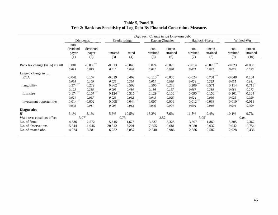
46

Table 5, Panel B. Test 2: Bank-tax Sensitivity of Log Debt By Financial Constraints Measure.

Dep. var.: Change in log long-term debt Dividends Credit ratings Kaplan-Zingales Hadlock-Pierce Whited-Wu

non-dividend

payer dividend

payer unrated rated con-

strained uncon-strained

con-strained

uncon-strained

con-strained

uncon-strained

(1) (2) (3) (4) (5) (6) (7) (8) (9) (10) Bank tax change (in %) at t =0 0.001 -0.036** -0.013 -0.046 0.024 -0.020 -0.014 -0.070*** -0.023 -0.030 0.015 0.015 0.015 0.040 0.021 0.028 0.021 0.022 0.022 0.023 Lagged change in … ROA -0.041 0.167 -0.019 0.462 -0.110** -0.005 -0.024 0.731*** -0.048 0.164 0.038 0.109 0.028 0.280 0.051 0.038 0.024 0.225 0.035 0.141 tangibility 0.374*** 0.272 0.362*** 0.502 0.506*** 0.253 0.209*** 0.571* 0.114 0.715** 0.123 0.238 0.095 0.480 0.136 0.197 0.067 0.288 0.084 0.272 firm size 0.174*** 0.107*** 0.124*** 0.315*** 0.129*** 0.100*** 0.090*** 0.150*** 0.101*** 0.104*** 0.021 0.037 0.023 0.062 0.043 0.025 0.024 0.036 0.025 0.029 investment opportunities 0.014*** -0.002 0.008*** 0.044*** 0.007 0.009** 0.012*** -0.038* 0.010** -0.011 0.003 0.011 0.003 0.013 0.006 0.004 0.004 0.019 0.004 0.009 Diagnostics R2 6.1% 8.1% 5.6% 10.5% 13.2% 7.6% 11.5% 9.4% 10.1% 9.7% Wald test: equal tax effect 3.97* 0.73 2.52 3.05* 0.04 No. of firms 4,536 2,572 5,615 1,675 3,327 3,325 3,307 1,860 3,305 2,367 No. of observations 15,644 11,946 20,542 7,201 7,655 9,681 9,080 9,037 9,042 8,754 No. of treated obs. 4,924 3,381 6,282 2,057 2,248 2,986 2,886 2,587 2,928 2,436

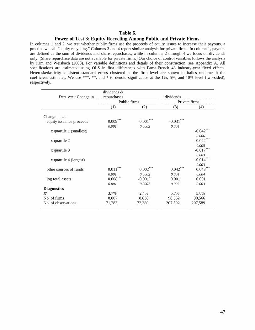
47

Table 6. Power of Test 3: Equity Recycling Among Public and Private Firms.

In columns 1 and 2, we test whether public firms use the proceeds of equity issues to increase their payouts, a practice we call “equity recycling.” Columns 3 and 4 report similar analysis for private firms. In column 1, payouts are defined as the sum of dividends and share repurchases, while in columns 2 through 4 we focus on dividends only. (Share repurchase data are not available for private firms.) Our choice of control variables follows the analysis by Kim and Weisbach (2008). For variable definitions and details of their construction, see Appendix A. All specifications are estimated using OLS in first differences with Fama-French 48 industry-year fixed effects. Heteroskedasticity-consistent standard errors clustered at the firm level are shown in italics underneath the coefficient estimates. We use ***, **, and * to denote significance at the 1%, 5%, and 10% level (two-sided), respectively.

Dep. var.: Change in… dividends & repurchases dividends

Public firms Private firms (1) (2) (3) (4) Change in … equity issuance proceeds 0.009*** 0.001*** -0.031*** 0.001 0.0002 0.004 x quartile 1 (smallest) -0.042*** 0.006 x quartile 2 -0.022*** 0.005 x quartile 3 -0.017*** 0.003 x quartile 4 (largest) -0.014*** 0.003 other sources of funds 0.011*** 0.002*** 0.042*** 0.043*** 0.001 0.0002 0.004 0.004 log total assets 0.008*** -0.001** 0.001 0.001 0.001 0.0002 0.003 0.003 Diagnostics R2 3.7% 2.4% 5.7% 5.8% No. of firms 8,807 8,838 98,562 98,566 No. of observations 71,283 72,380 207,592 207,589

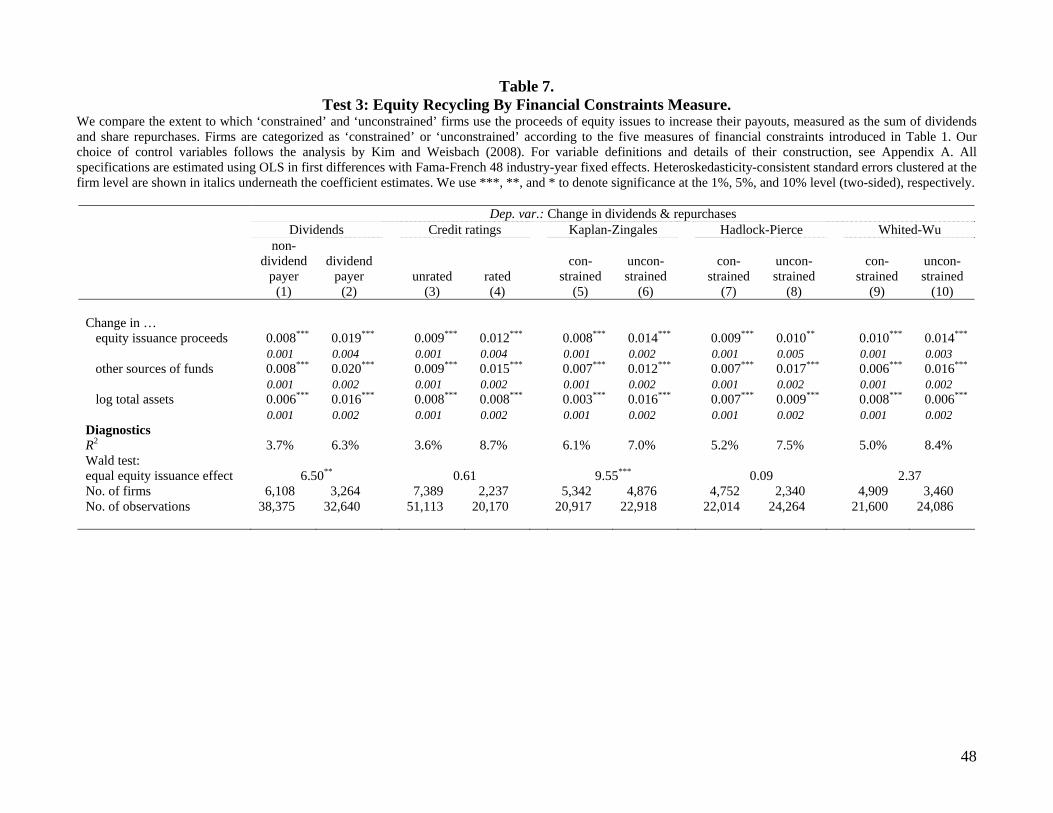
48

Table 7. Test 3: Equity Recycling By Financial Constraints Measure.

We compare the extent to which ‘constrained’ and ‘unconstrained’ firms use the proceeds of equity issues to increase their payouts, measured as the sum of dividends and share repurchases. Firms are categorized as ‘constrained’ or ‘unconstrained’ according to the five measures of financial constraints introduced in Table 1. Our choice of control variables follows the analysis by Kim and Weisbach (2008). For variable definitions and details of their construction, see Appendix A. All specifications are estimated using OLS in first differences with Fama-French 48 industry-year fixed effects. Heteroskedasticity-consistent standard errors clustered at the firm level are shown in italics underneath the coefficient estimates. We use ***, **, and * to denote significance at the 1%, 5%, and 10% level (two-sided), respectively.

Dep. var.: Change in dividends & repurchases Dividends Credit ratings Kaplan-Zingales Hadlock-Pierce Whited-Wu

non-dividend

payer dividend

payer unrated rated con-

strained uncon-strained

con-strained

uncon-strained

con-strained

uncon-strained

(1) (2) (3) (4) (5) (6) (7) (8) (9) (10) Change in … equity issuance proceeds 0.008*** 0.019*** 0.009*** 0.012*** 0.008*** 0.014*** 0.009*** 0.010** 0.010*** 0.014*** 0.001 0.004 0.001 0.004 0.001 0.002 0.001 0.005 0.001 0.003 other sources of funds 0.008*** 0.020*** 0.009*** 0.015*** 0.007*** 0.012*** 0.007*** 0.017*** 0.006*** 0.016*** 0.001 0.002 0.001 0.002 0.001 0.002 0.001 0.002 0.001 0.002 log total assets 0.006*** 0.016*** 0.008*** 0.008*** 0.003*** 0.016*** 0.007*** 0.009*** 0.008*** 0.006*** 0.001 0.002 0.001 0.002 0.001 0.002 0.001 0.002 0.001 0.002 Diagnostics R2 3.7% 6.3% 3.6% 8.7% 6.1% 7.0% 5.2% 7.5% 5.0% 8.4% Wald test: equal equity issuance effect 6.50** 0.61 9.55*** 0.09 2.37 No. of firms 6,108 3,264 7,389 2,237 5,342 4,876 4,752 2,340 4,909 3,460 No. of observations 38,375 32,640 51,113 20,170 20,917 22,918 22,014 24,264 21,600 24,086

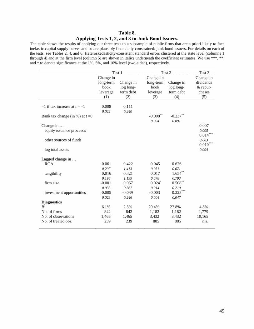
49

Table 8. Applying Tests 1, 2, and 3 to Junk Bond Issuers.

The table shows the results of applying our three tests to a subsample of public firms that are a priori likely to face inelastic capital supply curves and so are plausibly financially constrained: junk bond issuers. For details on each of the tests, see Tables 2, 4, and 6. Heteroskedasticity-consistent standard errors clustered at the state level (columns 1 through 4) and at the firm level (column 5) are shown in italics underneath the coefficient estimates. We use ***, **, and * to denote significance at the 1%, 5%, and 10% level (two-sided), respectively.

Test 1 Test 2 Test 3

Change in long-term

book leverage

Change in log long-term debt

Change in long-term

book leverage

Change in log long-term debt

Change in dividends & repur-chases

(1) (2) (3) (4) (5) =1 if tax increase at t = –1 0.008 0.111 0.022 0.240 Bank tax change (in %) at t =0 -0.008** -0.237** 0.004 0.091 Change in … 0.007 equity issuance proceeds 0.005 0.014*** other sources of funds 0.003 0.010*** log total assets 0.004 Lagged change in … ROA -0.061 0.422 0.045 0.626 0.207 1.413 0.051 0.671 tangibility 0.016 0.321 0.017 1.654** 0.196 1.199 0.078 0.793 firm size -0.001 0.067 0.024* 0.508** 0.033 0.367 0.014 0.210 investment opportunities -0.005 -0.039 -0.003 0.223*** 0.023 0.246 0.004 0.047 Diagnostics R2 6.1% 2.5% 20.4% 27.8% 4.8% No. of firms 842 842 1,182 1,182 1,779 No. of observations 1,465 1,465 3,432 3,432 10,165 No. of treated obs. 239 239 885 885 n.a.

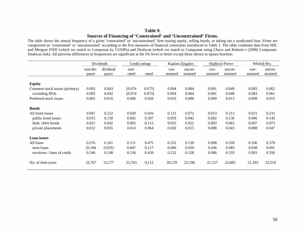
50

Table 9. Sources of Financing of ‘Constrained’ and ‘Unconstrained’ Firms.

The table shows the annual frequency of a given ‘constrained’ or ‘unconstrained’ firm issuing equity, selling bonds, or taking out a syndicated loan. Firms are categorized as ‘constrained’ or ‘unconstrained’ according to the five measures of financial constraints introduced in Table 1. The table combines data from SDC and Mergent FISD (which we match to Compustat by CUSIPs) and Dealscan (which we match to Compustat using Chava and Roberts’s (2008) Compustat-Dealscan link). All pairwise differences in frequencies are significant at the 5% level or better except those shown in square brackets. Dividends Credit ratings Kaplan-Zingales Hadlock-Pierce Whited-Wu

non-div.

payer dividend

payer non-rated rated

con-strained

uncon-strained

con-strained

uncon-strained

con-strained

uncon-strained

Equity Common stock issues (primary) 0.093 0.043 [0.074 0.075] 0.094 0.064 0.091 0.049 0.083 0.062 excluding IPOs 0.093 0.042 [0.074 0.074] 0.094 0.064 0.091 0.048 0.083 0.061 Preferred stock issues 0.002 0.016 0.006 0.026 0.016 0.006 0.009 0.013 0.009 0.015 Bonds All bond issues 0.047 0.222 0.020 0.416 0.121 0.072 0.013 0.213 0.021 0.231 public bond issues 0.015 0.158 0.002 0.307 0.059 0.042 0.002 0.136 0.006 0.143 Rule 144A bonds 0.025 0.042 0.005 0.112 0.053 0.022 0.003 0.063 0.007 0.073 private placements 0.012 0.055 0.014 0.064 0.026 0.015 0.008 0.043 0.008 0.047 Loan issues All loans 0.276 0.161 0.151 0.475 0.255 0.139 0.098 0.358 0.106 0.378 term loans [0.104 0.035] 0.047 0.117 0.080 0.029 0.036 0.083 0.038 0.091 revolvers / lines of credit 0.246 0.148 0.136 0.439 0.232 0.128 0.086 0.333 0.093 0.350 No. of firm-years 33,767 15,177 53,763 9,112 20,270 22,196 21,157 23,685 21,103 23,518

INTERNET APPENDIX

(NOT INTENDED FOR PUBLICATION)

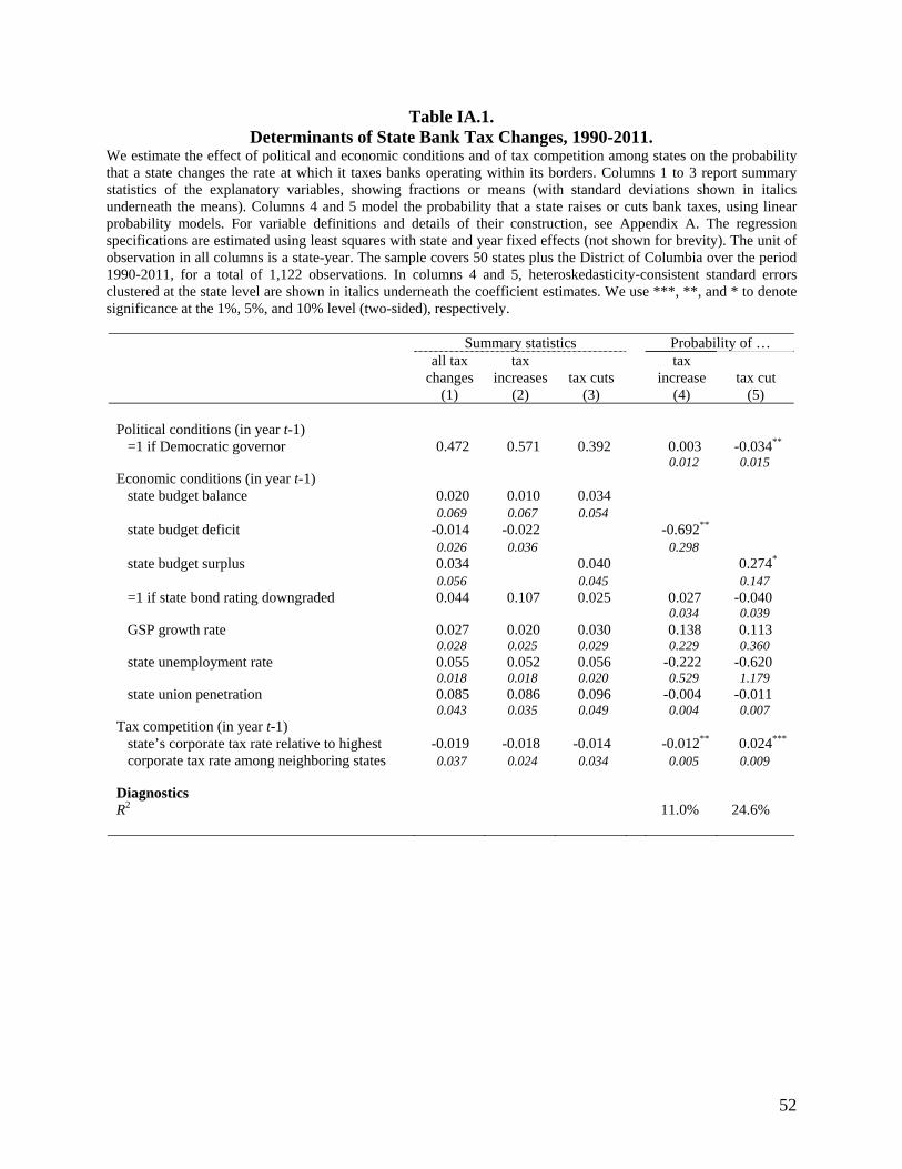
52

Table IA.1. Determinants of State Bank Tax Changes, 1990-2011.

We estimate the effect of political and economic conditions and of tax competition among states on the probability that a state changes the rate at which it taxes banks operating within its borders. Columns 1 to 3 report summary statistics of the explanatory variables, showing fractions or means (with standard deviations shown in italics underneath the means). Columns 4 and 5 model the probability that a state raises or cuts bank taxes, using linear probability models. For variable definitions and details of their construction, see Appendix A. The regression specifications are estimated using least squares with state and year fixed effects (not shown for brevity). The unit of observation in all columns is a state-year. The sample covers 50 states plus the District of Columbia over the period 1990-2011, for a total of 1,122 observations. In columns 4 and 5, heteroskedasticity-consistent standard errors clustered at the state level are shown in italics underneath the coefficient estimates. We use ***, **, and * to denote significance at the 1%, 5%, and 10% level (two-sided), respectively.

Summary statistics Probability of …

all tax

changes tax

increases tax cuts tax

increase tax cut (1) (2) (3) (4) (5) Political conditions (in year t-1) =1 if Democratic governor 0.472 0.571 0.392 0.003 -0.034** 0.012 0.015 Economic conditions (in year t-1) state budget balance 0.020 0.010 0.034 0.069 0.067 0.054 state budget deficit -0.014 -0.022 -0.692** 0.026 0.036 0.298 state budget surplus 0.034 0.040 0.274* 0.056 0.045 0.147 =1 if state bond rating downgraded 0.044 0.107 0.025 0.027 -0.040 0.034 0.039 GSP growth rate 0.027 0.020 0.030 0.138 0.113 0.028 0.025 0.029 0.229 0.360 state unemployment rate 0.055 0.052 0.056 -0.222 -0.620 0.018 0.018 0.020 0.529 1.179 state union penetration 0.085 0.086 0.096 -0.004 -0.011 0.043 0.035 0.049 0.004 0.007 Tax competition (in year t-1) state’s corporate tax rate relative to highest -0.019 -0.018 -0.014 -0.012** 0.024*** corporate tax rate among neighboring states 0.037 0.024 0.034 0.005 0.009 Diagnostics R2 11.0% 24.6%

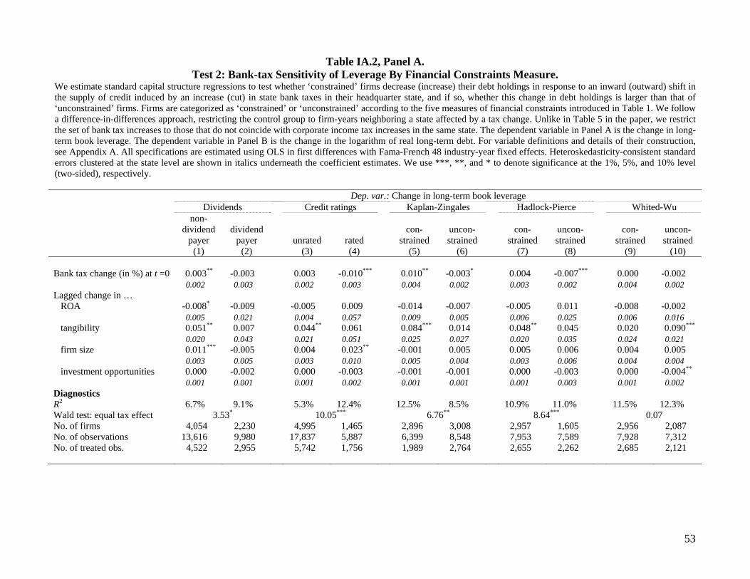
53

Table IA.2, Panel A. Test 2: Bank-tax Sensitivity of Leverage By Financial Constraints Measure.

We estimate standard capital structure regressions to test whether ‘constrained’ firms decrease (increase) their debt holdings in response to an inward (outward) shift in the supply of credit induced by an increase (cut) in state bank taxes in their headquarter state, and if so, whether this change in debt holdings is larger than that of ‘unconstrained’ firms. Firms are categorized as ‘constrained’ or ‘unconstrained’ according to the five measures of financial constraints introduced in Table 1. We follow a difference-in-differences approach, restricting the control group to firm-years neighboring a state affected by a tax change. Unlike in Table 5 in the paper, we restrict the set of bank tax increases to those that do not coincide with corporate income tax increases in the same state. The dependent variable in Panel A is the change in long-term book leverage. The dependent variable in Panel B is the change in the logarithm of real long-term debt. For variable definitions and details of their construction, see Appendix A. All specifications are estimated using OLS in first differences with Fama-French 48 industry-year fixed effects. Heteroskedasticity-consistent standard errors clustered at the state level are shown in italics underneath the coefficient estimates. We use ***, **, and * to denote significance at the 1%, 5%, and 10% level (two-sided), respectively. Dep. var.: Change in long-term book leverage Dividends Credit ratings Kaplan-Zingales Hadlock-Pierce Whited-Wu

non-dividend

payer dividend

payer unrated rated con-

strained uncon-strained

con-strained

uncon-strained

con-strained

uncon-strained

(1) (2) (3) (4) (5) (6) (7) (8) (9) (10) Bank tax change (in %) at t =0 0.003** -0.003 0.003 -0.010*** 0.010** -0.003* 0.004 -0.007*** 0.000 -0.002 0.002 0.003 0.002 0.003 0.004 0.002 0.003 0.002 0.004 0.002 Lagged change in … ROA -0.008* -0.009 -0.005 0.009 -0.014 -0.007 -0.005 0.011 -0.008 -0.002 0.005 0.021 0.004 0.057 0.009 0.005 0.006 0.025 0.006 0.016 tangibility 0.051** 0.007 0.044** 0.061 0.084*** 0.014 0.048** 0.045 0.020 0.090*** 0.020 0.043 0.021 0.051 0.025 0.027 0.020 0.035 0.024 0.021 firm size 0.011*** -0.005 0.004 0.023** -0.001 0.005 0.005 0.006 0.004 0.005 0.003 0.005 0.003 0.010 0.005 0.004 0.003 0.006 0.004 0.004 investment opportunities 0.000 -0.002 0.000 -0.003 -0.001 -0.001 0.000 -0.003 0.000 -0.004** 0.001 0.001 0.001 0.002 0.001 0.001 0.001 0.003 0.001 0.002 Diagnostics R2 6.7% 9.1% 5.3% 12.4% 12.5% 8.5% 10.9% 11.0% 11.5% 12.3% Wald test: equal tax effect 3.53* 10.05*** 6.76** 8.64*** 0.07 No. of firms 4,054 2,230 4,995 1,465 2,896 3,008 2,957 1,605 2,956 2,087 No. of observations 13,616 9,980 17,837 5,887 6,399 8,548 7,953 7,589 7,928 7,312 No. of treated obs. 4,522 2,955 5,742 1,756 1,989 2,764 2,655 2,262 2,685 2,121

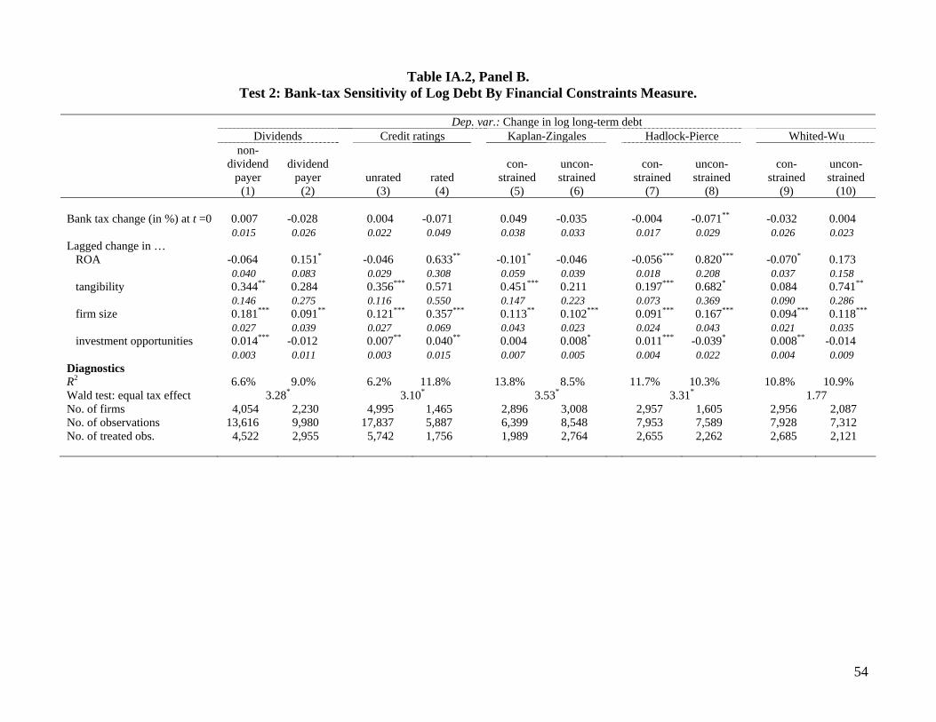
54

Table IA.2, Panel B. Test 2: Bank-tax Sensitivity of Log Debt By Financial Constraints Measure.

Dep. var.: Change in log long-term debt Dividends Credit ratings Kaplan-Zingales Hadlock-Pierce Whited-Wu

non-dividend

payer dividend

payer unrated rated con-

strained uncon-strained

con-strained

uncon-strained

con-strained

uncon-strained

(1) (2) (3) (4) (5) (6) (7) (8) (9) (10) Bank tax change (in %) at t =0 0.007 -0.028 0.004 -0.071 0.049 -0.035 -0.004 -0.071** -0.032 0.004 0.015 0.026 0.022 0.049 0.038 0.033 0.017 0.029 0.026 0.023 Lagged change in … ROA -0.064 0.151* -0.046 0.633** -0.101* -0.046 -0.056*** 0.820*** -0.070* 0.173 0.040 0.083 0.029 0.308 0.059 0.039 0.018 0.208 0.037 0.158 tangibility 0.344** 0.284 0.356*** 0.571 0.451*** 0.211 0.197*** 0.682* 0.084 0.741** 0.146 0.275 0.116 0.550 0.147 0.223 0.073 0.369 0.090 0.286 firm size 0.181*** 0.091** 0.121*** 0.357*** 0.113** 0.102*** 0.091*** 0.167*** 0.094*** 0.118*** 0.027 0.039 0.027 0.069 0.043 0.023 0.024 0.043 0.021 0.035 investment opportunities 0.014*** -0.012 0.007** 0.040** 0.004 0.008* 0.011*** -0.039* 0.008** -0.014 0.003 0.011 0.003 0.015 0.007 0.005 0.004 0.022 0.004 0.009 Diagnostics R2 6.6% 9.0% 6.2% 11.8% 13.8% 8.5% 11.7% 10.3% 10.8% 10.9% Wald test: equal tax effect 3.28* 3.10* 3.53* 3.31* 1.77 No. of firms 4,054 2,230 4,995 1,465 2,896 3,008 2,957 1,605 2,956 2,087 No. of observations 13,616 9,980 17,837 5,887 6,399 8,548 7,953 7,589 7,928 7,312 No. of treated obs. 4,522 2,955 5,742 1,756 1,989 2,764 2,655 2,262 2,685 2,121