Do Joint Audits Improve or Impair Audit Quality?

Mingcherng Deng

University of Minnesota

Tong Lu

University of Houston

Dan A. Simunic

University of British Columbia

Minlei Ye

University of Toronto

July 13, 2012

1

ABSTRACT

Joint audits involve two audit firms and may have the desired effect of “Two heads are

better than one.” However, joint audits may also induce one firm to free-ride on another

firm’s performance and therefore damage the total precision of audit evidence. In addition,

since joint audits involve two firms, it may be more expensive for the audited company to

“bribe” its auditors. However, adding another audit firm may create an “opinion shopping”

opportunity for the company, thereby threatening auditor independence. So the possible

consequences of joint audits are quite complex, and we incorporate these various trade-offs

in our analysis.

We investigate three regimes: single audits by a big firm; joint audits by two big firms;

joint audits by one big firm and one small firm. We compare the three regimes along three

dimensions: total audit evidence precision; auditor independence; and total audit fee. Our

analysis suggests that auditor independence is more likely to be compromised under joint

audits. Moreover, joint audits involving a technologically inefficient firm (a small firm) may

impair audit quality since a free-riding problem would prevail and result in lower total audit

evidence precision. Finally, audit fees under joint audits are lower than under single audits

when the technological difference between the two audit firms is small and/or the big firm

bears a large proportion of misstatement cost.

By providing the first theoretical study of joint audits, we advance understanding of

audit quality. We also generate a new set of empirically testable predictions and explain

current mixed empirical findings on joint audits.

Keywords: joint audit, audit quality, precision, auditor independence, audit fee.

2

1 Introduction

Are two heads better than one? The answer to this question seems straightforward

and it is exactly one of the reasons cited in support of joint audits, in which two audit firms

simultaneously and separately audit a company and jointly sign an audit report. Proponents

of joint audits argue that two pieces of audit evidence produce higher total information

precision than just a single piece. For example, in auditing a company’s fair value estimate

of a certain asset, auditors are weakly better off with another piece of audit evidence about

the fair value, because they always have the option of ignoring that piece of evidence if it is

completely uninformative.

Another benefit of joint audits may be to enhance auditor independence. The conven-

tional wisdom suggests that it is more expensive for a company to “bribe” two audit firms

in joint audits than a single firm in single audits. The reason is that, under joint audits,

the audit report must be co-signed by both firms and if one of the two refuses to sign, the

audit report cannot be released. This makes compromising auditor independence much more

difficult because the company has to pay a sufficiently large bribe to satisfy both audit firms.

Joint audits are not uncommon. For example, France has mandated by law joint audits

of public companies since 1966. The same thing is true for the financial services sector in

South Africa. Various countries, such as India, Germany, Switzerland, and the U.K., have

proposed voluntary joint audits. In 2010, the European Commission seriously considered

mandating joint audits, and continues to debate the issue at this time (EC (2010)).

If two heads were indeed better than one, and if two firms were more expensive to buy

off than one, then joint audits probably would be more prevalent in the world. However,

single audits are still the norm in significant portions of the world, with the U.S. being a

notable example. An interesting about-face change occurred in Denmark, which mandated

joint audits in 1930 but abolished this requirement in 2005.

3

Besides the benefits of joint audits, we identify two economic forces against joint audits

that are absent in the extant literature. The first one is free-riding. In joint audits, one of

the audit firms may save its auditing costs by investing less in its audit work and taking

advantage of the other audit firm’s hard work. In equilibrium, the precision of the audit

evidence is lower than that in the first-best world. The second one is auditor independence.

When a client intends to compromise audit evidence, joint audits provide an opportunity

of internal opinion shopping, because having more audit firms on board is like having more

draws in a lottery. Thus, joint audits can endanger auditor independence.

In theory, joint audits entail significant trade-offs in both audit evidence precision and

auditor independence, and in practice, the audit arrangements are diverse. Thus it is unclear

ex ante under what conditions joint audits dominate single audits and under what conditions

the converse is true.

We investigate the interactions among audit evidence precision, auditor independence,

and audit fee in three regimes: single audits by a big firm (Regime B); joint audits by two big

firms (Regime BB); joint audits by one big firm and one small firm (Regime BS). While the

first two regimes serve as benchmarks, the third regime is particularly interesting because it

is the European Commission’s target regime. Specifically, the European Commission states

that, Regime BS “could act as a catalyst for dynamising the audit market and allowing small

and medium-sized firms to participate more substantially in the segment of large audits” (EC

(2010), p.17). We make two assumptions to capture the differences between a big audit firm

and a small one. First, a big audit firm has an advantage in its auditing technology in

the sense that it has a lower marginal cost of audit evidence precision than a small firm.

Second, a big audit firm bears a larger proportion of misstatement cost (such as litigation

risk, reputation loss, etc.) than a small firm.

Comparing Regime BB with Regime B, we find the joint audit generates the same

4

audit evidence precision as the single audit. Though it costs more to compromise auditor

independence under the joint audit, the ex ante likelihood of non-independence is higher

under the joint audit. Audit fees are lower under the joint audit.

Regarding the differences between a single audit regime B and a joint audit regime BS,

we derive the same result regarding auditor independence as that in Regime BB: auditor

independence is more likely to be compromised, though it costs more to compromise inde-

pendence. Additionally, we find the total precision of audit evidence under joint audits is

lower than that under single audits. Furthermore, the audit fee under joint audit is less than

that under single audit if the big audit firm has a sufficiently small technological advantage

over the small firm and/or bears a large proportion of misstatement cost.

Our research contributes to several streams of literature. First, to our knowledge, there

has been no previous theoretical study of joint audits. Joint audits provide a unique setting

for analyzing both audit evidence precision and auditor independence, two components of

audit quality.

Second, we extend the theoretical literature on audit quality by introducing two new

strategic interactions into an auditing game. One is the company’s strategic shopping of

audit opinions between its two joint auditors. The other is the joint auditors’ strategic

free-riding incentives between each other. Previous research analyzed different factors that

may impair auditor independence (e.g., DeAngelo 1981a, Antle 1984, Simunic 1984, Magee

and Tseng 1990, Kanodia and Mukherji 1994, Lu 2006) or may influence audit information

precision/audit effort (Dye 1993, Pae and Yoo 2001, Schwartz 1997, Zhang 2007). These

papers focus on single audits. Our paper enriches the literature by studying joint audits and

thus identifying additional strategic factors.

Third, the existing empirical research provides mixed evidence on the impact of joint

audits on audit quality and audit fees (e.g., Francis et al. 2009, Gonthier-Besacier and Schatt

5

2007, Lesage et al. 2011, Piot 2007, Thinggaard and Kiertzner 2008). Our model helps

reconcile these findings and provides new empirical predictions, which we elaborate on in

Section 6.

Fourth, this study provides timely policy implications for regulators. To encourage the

growth of small-sized audit practices, the European Commission is considering mandating

large companies to hire at least one audit firm outside the Big-Four firms to conduct joint

audits (EC 2010). Our analysis suggests mandating joint audits with small audit firms for

the purpose of reducing market concentration could lead to detrimental effects on audit

quality. In light of the global convergence of accounting and auditing standards, this paper

can help inform regulators’ deliberations on joint audits.

The remainder of the paper proceeds as follows. Section 2 provides institutional back-

ground on how joint audits are conducted in practice. Section 3 presents the structure and

ingredients of the model under the three regimes, B, BB, and BS. Section 4 establishes the

equilibrium audit quality and audit fees in these regimes. Section 5 compares those regimes.

Section 6 develops the empirical predictions. We conclude in Section 7. We relegate all

proofs to the Appendix.

2 Institutional Background

This section explains the current joint audit practice in France to provide a foundation

for our model assumptions.1 Any listed company, any bank or other financial institution, and

any company that prepares consolidated financial statements is required by law in France

to appoint two different audit firms, who share the audit work and jointly sign the audit

report. The law has evolved into a professional standard of practice requiring a balanced

1This description is based on an interview of an audit firm senior partner conducted in Paris on 12/13/2011by one of the authors.

6

division of the work of both auditors in order to ensure an efficient dual control mechanism

(Gonthier-Besacier and Schatt 2007). However, in practice, auditors cannot always balance

their work allocation. For example, if both Big 4 auditors conduct joint audits for a large

listed company, then the workload sharing is likely to be balanced. But if one Big 4 firm

and one small audit firm conduct joint audits, it is harder to share the workload equally,

because the small audit firm cannot completely cover the client’s businesses (for instance, if

the small firm has no audit network abroad).

After accepting an audit engagement, the two audit firms first agree on their work

allocation. Their work is usually allocated either by regions (e.g., one audits America and

another audits Europe) or by divisions (business units). Then they start to audit the financial

statements simultaneously; they typically work this way because auditors need to meet a

deadline of finishing audit reports. After finishing their part of the audit, they review each

other’s audit work and prepare relevant documentation on the joint auditor’s working paper

review.

At the end of the audit, each joint auditor signs the audit report on the whole financial

statements, not just on the work he has done. However, courts evaluate each audit firm’s

responsibility based on auditing standards. Fault, if found, may not be at the same level

for each audit firm. For example, if the audited inventory is materially misstated, then

the auditor who is responsible for inventory could be held more responsible than the other

auditor, who simply reviewed the work.

These basic features of the French joint audit institutional regime—independent col-

lection of audit evidence by the two audit firms with a review of each other’s work, joint

agreement on the report to be issued, and separate and proportionate liability for unde-

tected material misstatements—are consistent with the assumptions of our model in the

next section.

7

3 Model

This section sets up the structure and ingredients of the model under three regimes:

single audits by a big firm (Regime B); joint audits by two big firms (Regime BB); joint

audits by one big firm and one small firm (Regime BS). In what follows, we first set up

the model for Regime B and then articulate how Regime BB and Regime BS deviate from

Regime B.

Regime B

Let x denote the fundamental value of a company,2 which is distributed normally with

mean x0 and precision h:

x ∼ N (x0,1

h). (1)

Since our focus is on both dimensions of audit quality, the precision of audit evidence and

auditor independence (DeAngelo (1981a)), we model both the audit evidence accumulation

process and the subsequent company-auditor negotiation.

The auditing technology or the audit evidence accumulation process produces audit

evidence yB about x:

yB|x ∼ N (x,1

eB), (2)

that is, conditional on x, yB is distributed normally with mean x and precision eB. In other

words, the audit evidence is an unbiased but noisy estimate of x.

An increase in the quantity of resources utilized by the auditor can reduce the noisiness

of or enhance the precision of audit evidence. To capture this effect, we assume that the

audit resource cost is kBC(e), where kB > 0 is a parameter and the precision e is a choice

2As a general rule in this paper, a symbol with a “˜” indicates a random variable and the same symbolwithout a “˜” indicates the realized value of that random variable. For example, x is a realized value of therandom variable x.

8

variable. We make the following standard assumptions about the cost function: C(0) = 0,

C ′ > 0 (but C ′(0) = 0), C ′′ > 0, and C ′′′ = 0. A quadratic function C(e) = e2, commonly

used in the literature, satisfies all of the above assumptions (Chan and Pae 1998, Laux and

Newman 2010, etc.).

To model the company-auditor negotiation, we introduce a pair of (Q, r) representing

the give-and-take between the company and its auditor. Specifically, a company may offer

or “bribe” its auditors an amount of Q in return for a certain report r the company prefers.

Following DeAngelo (1981a), we can also call Q “quasi-rent.”

An independent report, rI ≡ E[x|yB], is the auditor’s best estimate of x conditional on

the audit evidence yB. Note that rI is both informed and unbiased. However, if auditor

independence is compromised, the released report r will exceed rI . We assume that, when

auditor independence is compromised (when r > rI), r cannot exceed the observed audit

evidence. This can be justified by noting that the audit evidence documented in the audit

firms’ working papers is the only admissible evidence in court (Dye and Sridhar 2004).

Following the standard assumption in the literature (e.g., Antle and Nalebuff 1991, Dye

and Sridhar 2004), we assume that the audit firm will bear a loss of (r−x)2 if a misstatement

occurs, that is, if the certified report r is different from the company’s fundamental value x.

This misstatement cost includes possible legal liability and reputation loss resulting from an

audit failure.3

The sequence of events is as follows:

• The company offers a total audit fee of F and hires a big audit firm in a competitive

audit market. The company proposes an unaudited report r0 to its auditor.

3To focus on auditing issues, we abstract away from companies’ misstatement cost. If instead the com-panies’ legal liability and/or reputation loss due to misstatement is sufficiently high, the company may notpropose an inflated report in the first place, thereby making auditing a moot issue.

9

• The auditor chooses her desired precision eB of audit evidence in her audit plan.

• The audit evidence accumulation process produces audit evidence yB.

• The company-auditor negotiation determines a pair of (Q, r), where a company offers

or “bribes” its auditor an amount of Q in return for a certain audit report r.

• The company’s fundamental value x is realized and the auditor bears a misstatement

cost of (r − x)2.

The company’s payoff is its share price (which is assumed to be increasing in its audited

financial report r) net of its audit fee F and its “bribe” or quasi-rent Q paid to the auditor.

The auditor’s payoff is the receipt of F and Q net of the audit resource cost of kBC(eB) and

the misstatement cost of (r − x)2.

Regime BB and Regime BS

Having laid out the model setup for Regime B, we now turn to Regimes BB and BS.

The three regimes differ in the following ways:

• Regime B: The big audit firm has an audit resource cost function of kBC(e) and must

bear 100% of the misstatement cost.

• Regime BB: Each of the two big audit firms has an identical cost function of kBC(e)

and each must bear 50% of the misstatement cost.4 Additionally, we denote the audit

evidence accumulated by the two big firms yB and yB2, respectively.

• Regime BS: The big audit firm has a cost function of kBC(e) and the small audit firm

has a cost function of kSC(e), where kSkB

≡ m > 1 so that the big firm is more cost

4Alternatively, we assume one auditor shares α1 ∈ (0, 1) proportion of the misstatement cost and theother auditor shares α2 ∈ (0, 1), where α1+α2 = 1. We derive qualitative similar results, which are availableupon request.

10

efficient than the small firm. Furthermore, the big audit firm will bear a proportion of

αB and the small firm will bear a proportion of αS = 1−αB of the total misstatement

cost. We assume that the big audit firm bears a larger misstatement cost than the

small audit firm, i.e., αB > αS, consistent with DeAngelo (1981b). The assumptions

implies that αB ∈ (12, 1) and αS ∈ (0, 1

2). Additionally, we denote the audit evidence

accumulated by the big firm yB and that by the small firm yS.5

4 Equilibrium

Using backward induction, we analyze first the “bribe” or quasi-rent Q and the certified

report r, then the precision e of the audit evidence, and finally the audit fee F . In this

section, we lay out the equilibrium analyses for the three regimes B, BB, and BS. Section 5

compares the three regimes and gives a full explanation of the main results.

Before we begin, a discussion of the company’s initial unaudited report r0 is in order. In

our model, the company has an incentive to conduct earnings management to boost its report

and therefore initially it will propose a high unaudited report r0 to its auditors. Because it

is in the best interest of the company to propose a r0 as high as possible regardless of its

private information (if any), r0 is uninformative and so is ignored by the auditors. This is

true in our model whether or not the company has hidden information or not. Knowing that,

the auditors use their own informative evidence to estimate the company value. If instead a

company with hidden information could signal it by its real actions or by its audit fee, then

auditing would be moot. In a nutshell, we assume away the issue of the company’s signaling

in order to focus on the issue of external auditing, consistent with the literature (e.g., Antle

and Nalebuff (1991)).

5In practice, because of tight deadlines for the release of audited financial statements, joint audit firmsmust work simultaneously rather than sequentially. Therefore, we model the joint audit firms’ evidenceaccumulation processes as simultaneous moves.

11

4.1 Auditor Independence

In Regime B, at the stage of company-auditor negotiation about the final report to

be released, the audit evidence yB is already accumulated and documented in the auditor’s

working papers. The company may offer or “bribe” its auditor an amount of Q in return

for a certain audit report r which the company prefers. The pair of (Q, r) represents the

give-and-take between the company and its auditor.

The auditor weighs the amount of the quasi-rent Q she expects from the company against

her expectation of cost of misstatement (r−x)2. Because the auditor has already accumulated

audit evidence, her expectation is conditional on audit evidence, that is, E[(r−x)2|yB]. Recallthat the auditor always has an option of insisting on the independent report, rI ≡ E[x|yB].If she chooses to certify rI , her expectation of the misstatement cost will be E[(rI − x)2|yB].If she chooses to certify an inflated report r > rI , her expectation of the misstatement

cost will increase to E[(r − x)2|yB]. Naturally, to overcome the auditor’s objection to an

inflated report r > rI , the company must offer a Q large enough to cover the increase in

the misstatement cost, E[(r− x)2|yB]−E[(rI − x)2|yB]. In equilibrium, the company has no

incentive to overpay the auditor, so it will set Q equal to E[(r − x)2|yB]− E[(rI − x)2|yB].6

In general, the company wants to induce its auditor to certify a report as high as

possible. Because the audit evidence documented in the audit firm’s working papers is

the only admissible evidence in court, the audit report r cannot exceed the observed audit

evidence. Thus, if the audit evidence exceeds the independent report, (that is, yB > rI),

the company prefers to induce an audit report r = yB. This suggests that auditor non-

independence occurs when audit evidence exceeds the independent report, that is, yB >

rI . Therefore, the probability of auditor independence Pr(AI) is the probability that the

6We are interested in the probability of auditor independence when the budget constraint is not an issueto the company. Obviously, if the company were short of money to buy off its auditors in the first place,auditor independence would be a trivial issue.

12

independent report exceeds the audit evidence, i.e., Pr(rI > yB).

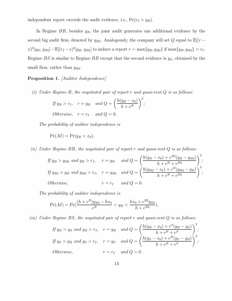
In Regime BB, besides yB, the joint audit generates one additional evidence by the

second big audit firm, denoted by yB2. Analogously, the company will set Q equal to E[(r−x)2|yB, yB2]−E[(rI −x)2|yB, yB2] to induce a report r = max{yB, yB2} if max{yB, yB2} > rI .

Regime BS is similar to Regime BB except that the second evidence is yS, obtained by the

small firm, rather than yB2.

Proposition 1. [Auditor Independence]

(i) Under Regime B, the negotiated pair of report r and quasi-rent Q is as follows:

If yB > rI, r = yB and Q =

(h(yB − x0)

h+ eB

)2

;

Otherwise, r = rI and Q = 0.

The probability of auditor independence is

Pr(AI) = Pr(yB < x0).

(ii) Under Regime BB, the negotiated pair of report r and quasi-rent Q is as follows:

If yB > yB2 and yB > rI, r = yB and Q =

(h(yB − x0) + eB2(yB − yB2)

h + eB + eB2

)2

;

If yB2 > yB and yB2 > rI , r = yB2 and Q =

(h(yB2 − x0) + eB(yB2 − yB)

h + eB + eB2

)2

;

Otherwise, r = rI and Q = 0.

The probability of auditor independence is

Pr(AI) = Pr((h+ eB)yB2 − hx0

eB< yB <

hx0 + eB2yB2

h+ eB2).

(iii) Under Regime BS, the negotiated pair of report r and quasi-rent Q is as follows:

If yB > yS and yB > rI, r = yB and Q =

(h(yB − x0) + eS(yB − yS)

h + eB + eS

)2

;

If yS > yB and yS > rI , r = yS and Q =

(h(yS − x0) + eB(yS − yB)

h + eB + eS

)2

;

Otherwise, r = rI and Q = 0.

13

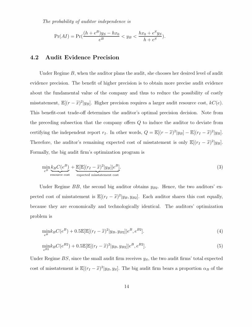
The probability of auditor independence is

Pr(AI) = Pr((h+ eB)yS − hx0

eB< yB <

hx0 + eSySh+ eS

).

4.2 Audit Evidence Precision

Under Regime B, when the auditor plans the audit, she chooses her desired level of audit

evidence precision. The benefit of higher precision is to obtain more precise audit evidence

about the fundamental value of the company and thus to reduce the possibility of costly

misstatement, E[(r − x)2|yB]. Higher precision requires a larger audit resource cost, kC(e).

This benefit-cost trade-off determines the auditor’s optimal precision decision. Note from

the preceding subsection that the company offers Q to induce the auditor to deviate from

certifying the independent report rI . In other words, Q = E[(r − x)2|yB] − E[(rI − x)2|yB].Therefore, the auditor’s remaining expected cost of misstatement is only E[(rI − x)2|yB].Formally, the big audit firm’s optimization program is

mineB

kBC(eB)︸ ︷︷ ︸resource cost

+ E[E[(rI − x)2|yB]|eB]︸ ︷︷ ︸expected misstatement cost

. (3)

Under Regime BB, the second big auditor obtains yB2. Hence, the two auditors’ ex-

pected cost of misstatement is E[(rI − x)2|yB, yB2]. Each auditor shares this cost equally,

because they are economically and technologically identical. The auditors’ optimization

problem is

mineB

kBC(eB) + 0.5E[E[(rI − x)2|yB, yB2]|eB, eB2]. (4)

mineB2

kBC(eB2) + 0.5E[E[(rI − x)2|yB, yB2]|eB, eB2]. (5)

Under Regime BS, since the small audit firm receives yS, the two audit firms’ total expected

cost of misstatement is E[(rI − x)2|yB, yS]. The big audit firm bears a proportion αB of the

14

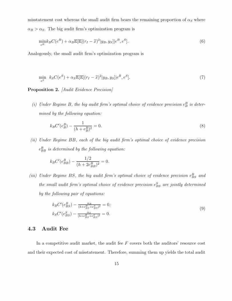
misstatement cost whereas the small audit firm bears the remaining proportion of αS where

αB > αS. The big audit firm’s optimization program is

mineB

kBC(eB) + αBE[E[(rI − x)2|yB, yS]|eB, eS]. (6)

Analogously, the small audit firm’s optimization program is

mineS

kSC(eS) + αSE[E[(rI − x)2|yB, yS]|eB, eS]. (7)

Proposition 2. [Audit Evidence Precision]

(i) Under Regime B, the big audit firm’s optimal choice of evidence precision eBB is deter-

mined by the following equation:

kBC′(eBB)−

1

(h+ eBB)2= 0. (8)

(ii) Under Regime BB, each of the big audit firm’s optimal choice of evidence precision

eBBB is determined by the following equation:

kBC′(eBBB)−

1/2

(h+ 2eBBB)2= 0.

(iii) Under Regime BS, the big audit firm’s optimal choice of evidence precision eBBS and

the small audit firm’s optimal choice of evidence precision eSBS are jointly determined

by the following pair of equations:

kBC′(eBBS)− αB

(h+eBBS+eSBS)2 = 0;

kSC′(eSBS)− αS

(h+eBBS+eSBS)2 = 0.

(9)

4.3 Audit Fee

In a competitive audit market, the audit fee F covers both the auditors’ resource cost

and their expected cost of misstatement. Therefore, summing them up yields the total audit

15

fees in each regime:

F = kBC(eB) + E[E[(rI − x)2|yB]|eB]. (10)

F = kBC(eB) + kBC(eB2) + E[E[(rI − x)2|yB, yB2]|eB, eB2]. (11)

F = kBC(eB) + kSC(eS) + E[E[(rI − x)2|yB, yS]|eB, eS]. (12)

Proposition 3. [Audit Fee]

(i) Under Regime B, the equilibrium total audit fee FB is as follows:

FB = kBC(eBB) +1

h + eBB. (13)

(ii) Under Regime BB, the equilibrium total audit fee FBB is as follows:

FBB = 2kBC(eBBB) +1

h+ 2eBBB

. (14)

(iii) Under Regime BS, the equilibrium total audit fee FBS is as follows:

FBS = kBC(eBBS) + kSC(eSBS) +1

h+ eBBS + eSBS

. (15)

5 Comparison

Having derived the results on auditor independence, audit evidence precision, and audit

fee, now we are ready to compare Regimes B, BB, and BS along those three dimensions.

5.1 Audit Evidence Precision

To facilitate comparisons among Regimes B, BB, and BS, we juxtapose the optimal

choices of audit evidence precision given in Proposition 2 in the following table.

16

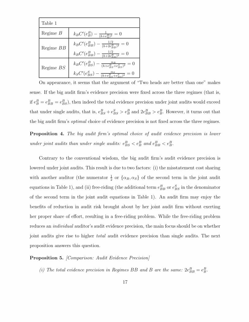
Table 1

Regime B kBC′(eBB)− 1

(h+eBB)2= 0

Regime BBkBC

′(eBBB)− 1/2

(h+2eBBB)2= 0

kBC′(eBBB)− 1/2

(h+2eBBB)2= 0

Regime BSkBC

′(eBBS)− αB

(h+eBBS+eSBS)2 = 0

kSC′(eSBS)− αS

(h+eBBS+eSBS)2 = 0

On appearance, it seems that the argument of “Two heads are better than one” makes

sense. If the big audit firm’s evidence precision were fixed across the three regimes (that is,

if eBB = eBBB = eBBS), then indeed the total evidence precision under joint audits would exceed

that under single audits, that is, eBBS + eSBS > eBB and 2eBBB > eBB. However, it turns out that

the big audit firm’s optimal choice of evidence precision is not fixed across the three regimes.

Proposition 4. The big audit firm’s optimal choice of audit evidence precision is lower

under joint audits than under single audits: eBBS < eBB and eBBB < eBB.

Contrary to the conventional wisdom, the big audit firm’s audit evidence precision is

lowered under joint audits. This result is due to two factors: (i) the misstatement cost sharing

with another auditor (the numerator 12or {αB, αS} of the second term in the joint audit

equations in Table 1), and (ii) free-riding (the additional term eBBB or eSBS in the denominator

of the second term in the joint audit equations in Table 1). An audit firm may enjoy the

benefits of reduction in audit risk brought about by her joint audit firm without exerting

her proper share of effort, resulting in a free-riding problem. While the free-riding problem

reduces an individual auditor’s audit evidence precision, the main focus should be on whether

joint audits give rise to higher total audit evidence precision than single audits. The next

proposition answers this question.

Proposition 5. [Comparison: Audit Evidence Precision]

(i) The total evidence precision in Regimes BB and B are the same: 2eBBB = eBB.

17

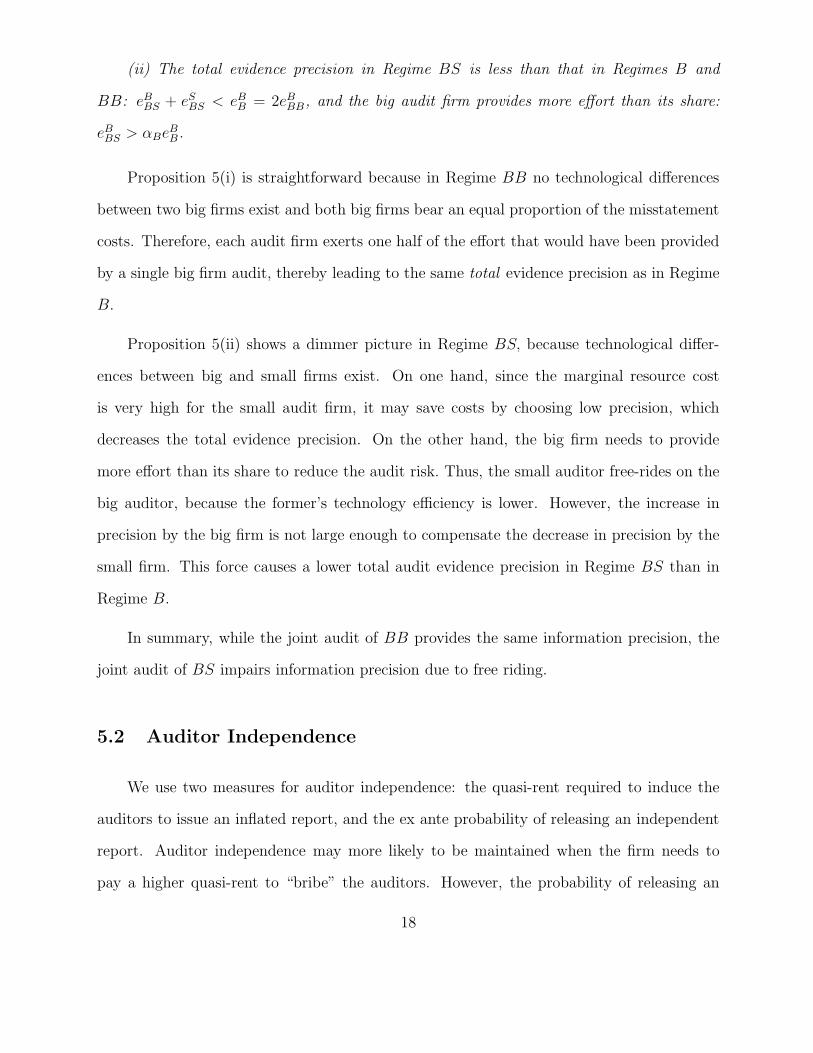
(ii) The total evidence precision in Regime BS is less than that in Regimes B and

BB: eBBS + eSBS < eBB = 2eBBB, and the big audit firm provides more effort than its share:

eBBS > αBeBB.

Proposition 5(i) is straightforward because in Regime BB no technological differences

between two big firms exist and both big firms bear an equal proportion of the misstatement

costs. Therefore, each audit firm exerts one half of the effort that would have been provided

by a single big firm audit, thereby leading to the same total evidence precision as in Regime

B.

Proposition 5(ii) shows a dimmer picture in Regime BS, because technological differ-

ences between big and small firms exist. On one hand, since the marginal resource cost

is very high for the small audit firm, it may save costs by choosing low precision, which

decreases the total evidence precision. On the other hand, the big firm needs to provide

more effort than its share to reduce the audit risk. Thus, the small auditor free-rides on the

big auditor, because the former’s technology efficiency is lower. However, the increase in

precision by the big firm is not large enough to compensate the decrease in precision by the

small firm. This force causes a lower total audit evidence precision in Regime BS than in

Regime B.

In summary, while the joint audit of BB provides the same information precision, the

joint audit of BS impairs information precision due to free riding.

5.2 Auditor Independence

We use two measures for auditor independence: the quasi-rent required to induce the

auditors to issue an inflated report, and the ex ante probability of releasing an independent

report. Auditor independence may more likely to be maintained when the firm needs to

pay a higher quasi-rent to “bribe” the auditors. However, the probability of releasing an

18

independent report is a more direct measure of auditor independence.

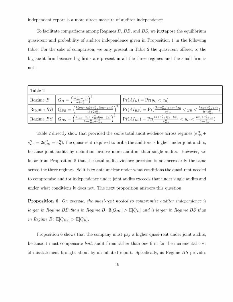
To facilitate comparisons among Regimes B, BB, and BS, we juxtapose the equilibrium

quasi-rent and probability of auditor independence given in Proposition 1 in the following

table. For the sake of comparison, we only present in Table 2 the quasi-rent offered to the

big audit firm because big firms are present in all the three regimes and the small firm is

not.

Table 2

Regime B QB =(

h(yB−x0)

h+eBB

)2

Pr(AIB) = Pr(yB < x0)

Regime BB QBB =(

h(yB−x0)+eBBB(yB−yB2)

h+2eBBB

)2

Pr(AIBB) = Pr((h+eBBB)yB2−hx0

eBBB< yB <

hx0+eBBByB2

h+eBBB)

Regime BS QBS =(

h(yB−x0)+eSBS(yB−yS)

h+eBBS+eSBS

)2

Pr(AIBS) = Pr((h+eBBS)yS−hx0

eBBS< yB <

hx0+eSBSySh+eSBS

)

Table 2 directly show that provided the same total audit evidence across regimes (eBBS+

eSBS = 2eBBB = eBB), the quasi-rent required to bribe the auditors is higher under joint audits,

because joint audits by definition involve more auditors than single audits. However, we

know from Proposition 5 that the total audit evidence precision is not necessarily the same

across the three regimes. So it is ex ante unclear under what conditions the quasi-rent needed

to compromise auditor independence under joint audits exceeds that under single audits and

under what conditions it does not. The next proposition answers this question.

Proposition 6. On average, the quasi-rent needed to compromise auditor independence is

larger in Regime BB than in Regime B: E[QBB ] > E[QB] and is larger in Regime BS than

in Regime B: E[QBS ] > E[QB ].

Proposition 6 shows that the company must pay a higher quasi-rent under joint audits,

because it must compensate both audit firms rather than one firm for the incremental cost

of misstatement brought about by an inflated report. Specifically, as Regime BS provides

19

lower information precision than Regime B, the expected misstatement cost is higher in

Regime BS. Thus, it costs more for the firm to induce the auditors to compromise their

independence in joint audits.

Next we move on to investigate the probability of auditor independence across the three

regimes.

Proposition 7. The likelihood of auditor independence under a joint audit is lower than

that under single audit: Pr(AIBS) < Pr(AIB) and Pr(AIBB) < Pr(AIB).

The result of Proposition 7 may sound surprising. If it is more expensive to buy off two

auditors, why would the probability of auditor independence be lower under joint audits?

This is because joint audits provide companies an opportunity of internal opinion shopping

between auditors for a favorable audit opinion. But such an opportunity does not exist under

single audits.

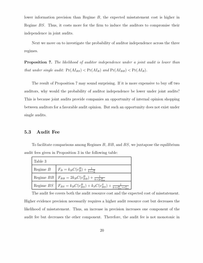
5.3 Audit Fee

To facilitate comparisons among Regimes B, BB, and BS, we juxtapose the equilibrium

audit fees given in Proposition 3 in the following table:

Table 3

Regime B FB = kBC(eBB) +1

h+eBB

Regime BB FBB = 2kBC(eBBB) +1

h+2eBBB

Regime BS FBS = kBC(eBBS) + kSC(eSBS) +1

h+eBBS+eSBS

The audit fee covers both the audit resource cost and the expected cost of misstatement.

Higher evidence precision necessarily requires a higher audit resource cost but decreases the

likelihood of misstatement. Thus, an increase in precision increases one component of the

audit fee but decreases the other component. Therefore, the audit fee is not monotonic in

20

audit precision and it is not ex ante straightforward to rank the audit fees across the three

regimes.

Proposition 8. [Comparison: Audit Fee]

(i) The audit fee in Regime BB is lower than that in Regime B: FBB < FB.

(ii) The audit fee in Regime BS is lower than that in Regime B if and only if the big

firm and small firm have similar technology efficiency and/or the big firm bears a sufficiently

large proportion of misstatement cost: there exists a m† > 1 such that FBS < FB for m < m†

and there exists an 12< α† < 1 such that FBS < FB for αB > α†.

Proposition 8(i) states that the total audit fee under joint audits by two big firms is

lower than that under single audits by a big firm. This result is due to the convexity of the

resource cost function, a standard assumption in economics. For example, one audit firm

doing all the work under a completion time constraint (Regime B) may experience a higher

level of staff supervision and coordination costs than if the work was split between firms

(Regime BB).

Proposition 8(ii) ranks the audit fees across the alternative regimes in the dimension of

the audit firms’ technological advantage and share of misstatement costs. Recall that the

small audit firm suffers technological inefficiency in the sense that its marginal resource cost

is larger than the big firm’s, that is, kSkB

≡ m > 1, where m represent the extent of the small

firm’s technological inefficiency. When the small audit firm’s marginal resource cost is higher

(a larger m), its audit resource cost is higher. Moreover, the small audit firm chooses lower

audit evidence precision, which subsequently leads to a higher likelihood of misstatement.

As a result of these two factors, the total audit fee in Regime BS will be higher than its

counterpart in Regime B when m is sufficiently large. By the same reasoning, the converse

is true when m is sufficiently small, that is, the audit fee in Regime BS is lower than that

in Regime B if the big firm and small firm have similar technology efficiency.

21

Second, when αB is sufficiently large, the big firm has a large incentive to boost her

precision because she bears a large proportion of misstatement cost. This implies a large

total audit evidence precision and thus a small misstatement cost, which is reflected in the

total audit fee. In brief, the total audit fee in Regime BS is lower than that in Regime B

when the big firm bears a sufficiently large proportion of misstatement cost. Additionally, as

αB continues to increases, the increase of resource cost from higher precision will dominate

the reduction of misstatement cost, causing the increase of audit fees. In the extreme case

when αB = 1, the audit fee is identical under two regimes.

6 Empirical Prediction

Our model produces two sets of empirically testable predictions about joint audits on

audit quality (Propositions 4 to 7) and audit fees (Proposition 8). In this section, we explain

how our predictions make additional new testable hypotheses and how our predictions shed

light on the extant empirical evidence.

Our model shows that audit quality (audit evidence precision and auditor independence)

can be impaired or improved under various conditions. Indeed, Lesage et al. (2011) find no

stable relationship between joint audits and abnormal accruals. Using theoretical analysis,

we come up with the conditions under which audit quality is likely to be impaired and the

conditions under which audit quality is likely to be improved.

Audit Quality.

Audit quality is determined by both audit evidence precision and auditor independence

(DeAngelo 1981a). To our knowledge, there has not been any research directly examining

the impact of joint audits on auditor independence. Propositions 6 and 7 together suggest

that though it is more expensive to induce non-independence under joint audits than single

22

audits, if companies’ budgetary constraints are not binding, the ex ante probability of non-

independence is higher under joint audits than under single audits. This is a new testable

hypothesis we produce.

Our analysis on evidence precision generates the following predictions: (1) two audit

firms whose technology efficiency are comparable can provide the same audit quality as a

single firm audit (Proposition 5 (i)); (2) adding a firm with lower technology efficiency to

form a joint audit will reduce audit quality (Proposition 5 (ii)). We find these predictions

are supported by several empirical studies. For example, Holm and Thinggaard (2010)

find that there is no difference in the auditors’ ability to constrain earnings management

between joint and single audits in general. Using a sample of 177 French listed companies

on December 31, 2003, Marmousez (2008) provides evidence that the presence of two Big 4

audit firms is associated with lower reporting quality. If one of the Big 4 firms is an industry

specialist and the other is not, we can interpret the non-specialist firm as one that has lower

technology efficiency, and therefore this empirical evidence is consistent with our prediction

in Proposition 5(ii).

More generally, our analysis implies that adding a more efficient auditor can improve

audit quality, which is supported by Francis et al. (2009). They examine auditor choice for

listed companies in France. They find that companies using one Big 4 auditor paired with a

non-Big 4 auditor have smaller income-increasing abnormal accruals compared to companies

that use no Big 4 auditors and this effect is even stronger for companies that use two Big 4

auditors.

However, using a disclosure score for companies composing the French SBF 120 index

from 2006 to 2009, Paugam and Casta (2012) provide evidence that the combination of

Big 4/non-Big 4 auditors generate higher impairment-related disclosures levels than other

combinations, i.e., two Big 4 or two non-Big 4. This result is inconsistent with Proposition

23

5 (ii), but it could be due to the auditor independence effect.

Therefore, we conjecture these empirical studies mainly capture the audit evidence pre-

cision aspect of audit quality. We suggest that care must be taken to separate empirically

the effect of audit evidence precision and that of auditor independence.

Audit Fee. Proposition 8(i) proposes that the total audit fee under joint audits by two

big firms is lower than that under single audits by one big firm. The empirical evidence is

consistent with the direction of our prediction. Gonthier-Besacier and Schatt (2007) find that

when two Big Four firms audit company accounts, the fees charged (adjusted for company

size) are significantly lower in comparison with those paid in the other cases (BS or two

small audit firms). Francis et al. (2009) find French audit fees are not higher under joint

audits compared to other European countries that do not require joint audits.

However, Proposition 8 (ii) predicts that when a small firm is involved in joint audits,

the comparison is not clear-cut. Indeed, Lesage et al. (2011) confirm the absence of any

stable relationship between joint audit and audit fees. Thinggaard and Kiertzner (2008)

examines audit fees paid by all 126 non-financial companies listed on the Copenhagen Stock

Exchange in 2002. They find that joint audits reduce audit fees compared with audits where

one auditor is dominant, albeit only for larger companies. However, the opposite evidence

is documented in a different setting by Holm and Thinggaard (2010). They use the data

for the whole population of non-financial Danish companies listed on the Copenhagen Stock

Exchange in the five-year period surrounding the abolishment of joint audit in 2005. They

find discounts (of around 25%) in audit fees in companies that change to single audits.

Moreover, we discover that when joint auditors bear the same proportion of misstate-

ment cost, the total audit fee under Regime BS exceeds that under Regime BB because

of small auditors’ technology inefficiency (see the proof of Proposition 8). Consistent with

this prediction, Audousset-Coulier (2012) shows the joint audits by two big auditors do not

24

require a fee premium compared to joint audits by one big firm and one small firm.

7 Conclusion

To restore trust in financial reporting, in the wake of the recent financial crisis, the Eu-

ropean Commission, among others, is re-examining the role of auditing. One of its proposed

actions is to mandate joint audits. However, it is ex-ante unclear whether joint audits are

more beneficial than single audits. Though two heads may be better than one, free-riding

can reduce the information precision produced by audits. Regarding auditor independence,

it may be more expensive to buy off two parties than one, but adding another audit firm

allows the client the opportunity of shopping for a more favorable opinion.

We develop a theory of joint audits that incorporates these trade-offs and solve for the

equilibrium solution. We compare joint audits by two big firms and joint audits by one big

firm and one small firm with single audits by a big firm. Three dimensions are examined:

audit evidence precision, auditor independence, and audit fees.

We find that the benefits of joint audit do not always dominate its costs. Besides the

out-of-pocket audit resource costs, we need to consider the more significant indirect costs

of joint audits: free-riding, which may decrease the precision of the audit evidence; internal

opinion shopping, which may compromise auditor independence. Though it is more expensive

to compromise auditor independence under joint audits, joint audits provide an additional

opportunity for a company to shop for a better audit opinion. If companies’ budgets are

not binding (i.e., they can afford the “bribe” needed to get the report they want), auditor

independence is more likely to be compromised under joint audits.

Therefore, the answer to the question “Do joint audits improve or impair audit quality?”

is “It depends.” In this paper, we identify the conditions under which joint audits improve

25

audit quality and the conditions under which they impair audit quality. Our research ex-

tends the theoretical literature on audit quality and provides timely policy implications to

regulators. Our model provides a theoretical framework that can explain the seemingly in-

consistent and diverse empirical findings to date, and the propositions we develop provide

further predictions that can potentially be tested empirically.

26

Appendix

Proof of Proposition 1

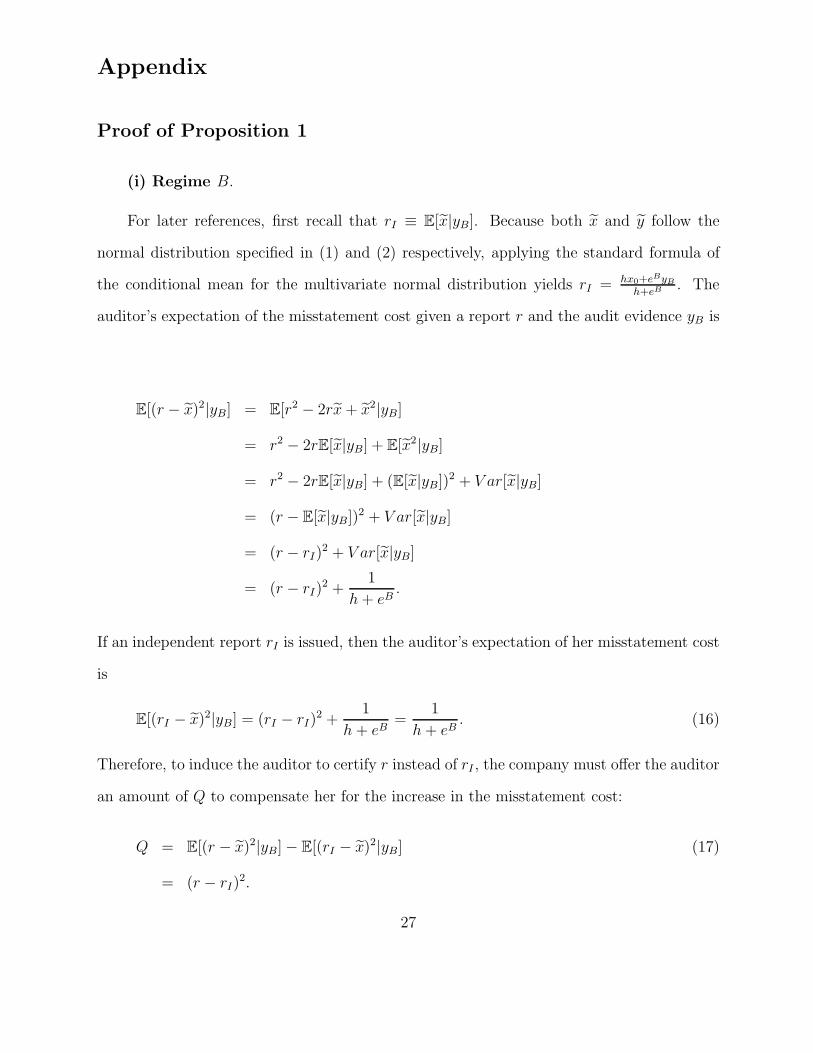
(i) Regime B.

For later references, first recall that rI ≡ E[x|yB]. Because both x and y follow the

normal distribution specified in (1) and (2) respectively, applying the standard formula of

the conditional mean for the multivariate normal distribution yields rI = hx0+eByBh+eB

. The

auditor’s expectation of the misstatement cost given a report r and the audit evidence yB is

E[(r − x)2|yB] = E[r2 − 2rx+ x2|yB]

= r2 − 2rE[x|yB] + E[x2|yB]

= r2 − 2rE[x|yB] + (E[x|yB])2 + V ar[x|yB]

= (r − E[x|yB])2 + V ar[x|yB]

= (r − rI)2 + V ar[x|yB]

= (r − rI)2 +

1

h+ eB.

If an independent report rI is issued, then the auditor’s expectation of her misstatement cost

is

E[(rI − x)2|yB] = (rI − rI)2 +

1

h + eB=

1

h+ eB. (16)

Therefore, to induce the auditor to certify r instead of rI , the company must offer the auditor

an amount of Q to compensate her for the increase in the misstatement cost:

Q = E[(r − x)2|yB]− E[(rI − x)2|yB] (17)

= (r − rI)2.

27

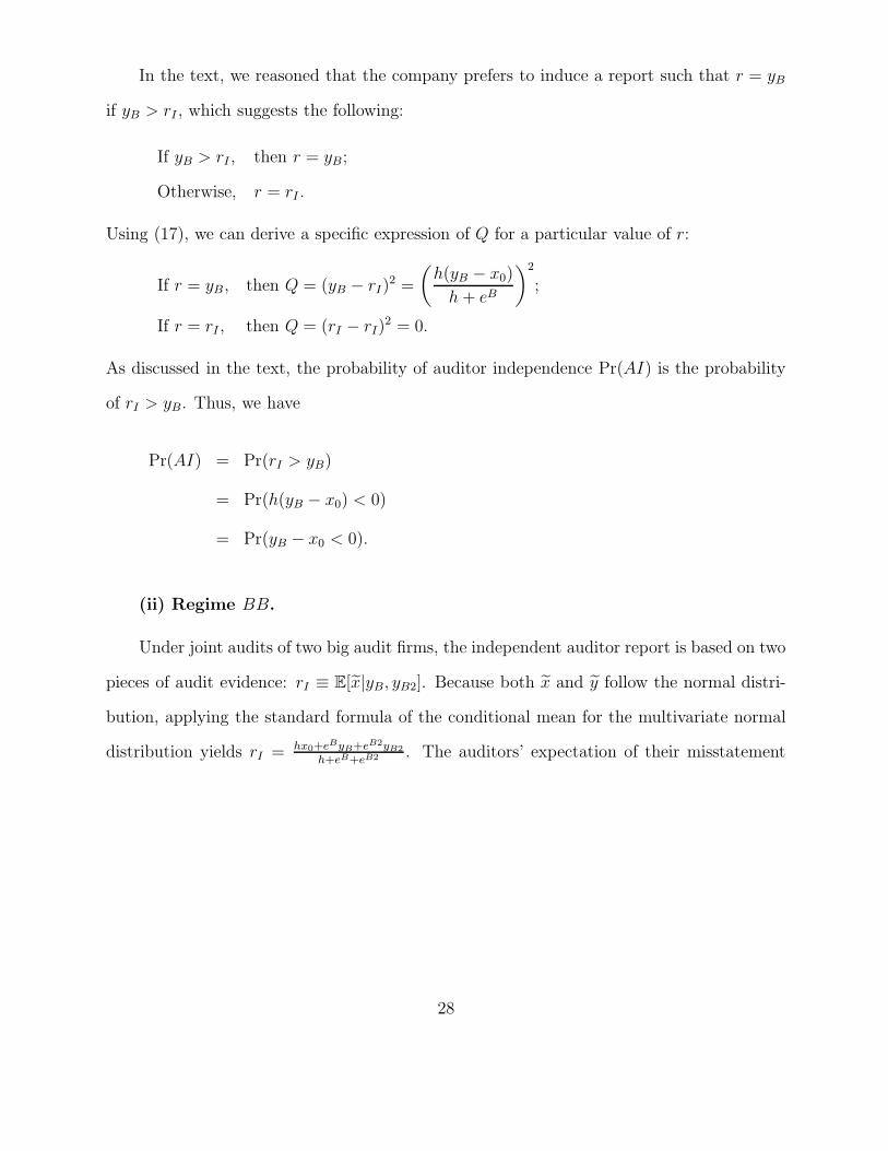
In the text, we reasoned that the company prefers to induce a report such that r = yB

if yB > rI , which suggests the following:

If yB > rI , then r = yB;

Otherwise, r = rI .

Using (17), we can derive a specific expression of Q for a particular value of r:

If r = yB, then Q = (yB − rI)2 =

(h(yB − x0)

h+ eB

)2

;

If r = rI , then Q = (rI − rI)2 = 0.

As discussed in the text, the probability of auditor independence Pr(AI) is the probability

of rI > yB. Thus, we have

Pr(AI) = Pr(rI > yB)

= Pr(h(yB − x0) < 0)

= Pr(yB − x0 < 0).

(ii) Regime BB.

Under joint audits of two big audit firms, the independent auditor report is based on two

pieces of audit evidence: rI ≡ E[x|yB, yB2]. Because both x and y follow the normal distri-

bution, applying the standard formula of the conditional mean for the multivariate normal

distribution yields rI = hx0+eByB+eB2yB2

h+eB+eB2 . The auditors’ expectation of their misstatement

28

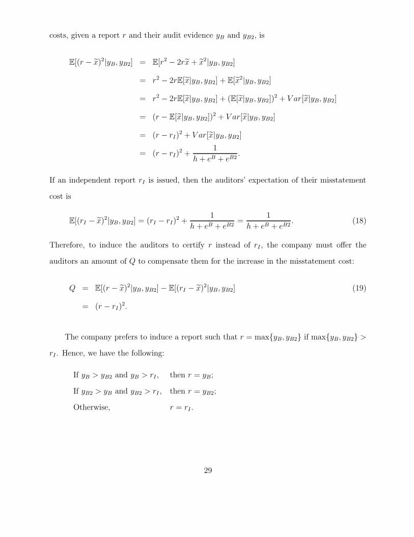
costs, given a report r and their audit evidence yB and yB2, is

E[(r − x)2|yB, yB2] = E[r2 − 2rx+ x2|yB, yB2]

= r2 − 2rE[x|yB, yB2] + E[x2|yB, yB2]

= r2 − 2rE[x|yB, yB2] + (E[x|yB, yB2])2 + V ar[x|yB, yB2]

= (r − E[x|yB, yB2])2 + V ar[x|yB, yB2]

= (r − rI)2 + V ar[x|yB, yB2]

= (r − rI)2 +

1

h+ eB + eB2.

If an independent report rI is issued, then the auditors’ expectation of their misstatement

cost is

E[(rI − x)2|yB, yB2] = (rI − rI)2 +

1

h + eB + eB2=

1

h+ eB + eB2. (18)

Therefore, to induce the auditors to certify r instead of rI , the company must offer the

auditors an amount of Q to compensate them for the increase in the misstatement cost:

Q = E[(r − x)2|yB, yB2]− E[(rI − x)2|yB, yB2] (19)

= (r − rI)2.

The company prefers to induce a report such that r = max{yB, yB2} if max{yB, yB2} >

rI . Hence, we have the following:

If yB > yB2 and yB > rI , then r = yB;

If yB2 > yB and yB2 > rI , then r = yB2;

Otherwise, r = rI .

29

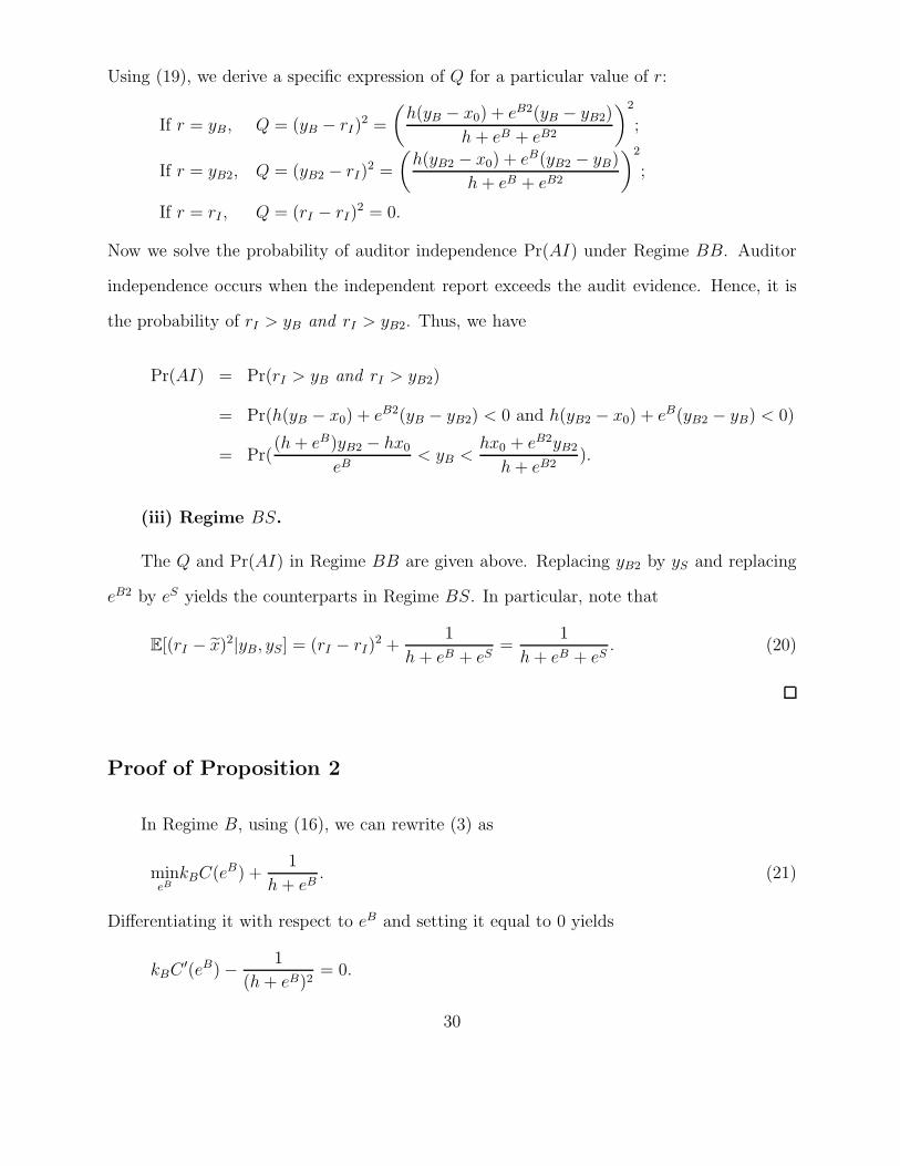
Using (19), we derive a specific expression of Q for a particular value of r:

If r = yB, Q = (yB − rI)2 =

(h(yB − x0) + eB2(yB − yB2)

h+ eB + eB2

)2

;

If r = yB2, Q = (yB2 − rI)2 =

(h(yB2 − x0) + eB(yB2 − yB)

h+ eB + eB2

)2

;

If r = rI , Q = (rI − rI)2 = 0.

Now we solve the probability of auditor independence Pr(AI) under Regime BB. Auditor

independence occurs when the independent report exceeds the audit evidence. Hence, it is

the probability of rI > yB and rI > yB2. Thus, we have

Pr(AI) = Pr(rI > yB and rI > yB2)

= Pr(h(yB − x0) + eB2(yB − yB2) < 0 and h(yB2 − x0) + eB(yB2 − yB) < 0)

= Pr((h+ eB)yB2 − hx0

eB< yB <

hx0 + eB2yB2

h+ eB2).

(iii) Regime BS.

The Q and Pr(AI) in Regime BB are given above. Replacing yB2 by yS and replacing

eB2 by eS yields the counterparts in Regime BS. In particular, note that

E[(rI − x)2|yB, yS] = (rI − rI)2 +

1

h + eB + eS=

1

h+ eB + eS. (20)

Proof of Proposition 2

In Regime B, using (16), we can rewrite (3) as

mineB

kBC(eB) +1

h+ eB. (21)

Differentiating it with respect to eB and setting it equal to 0 yields

kBC′(eB)− 1

(h+ eB)2= 0.

30

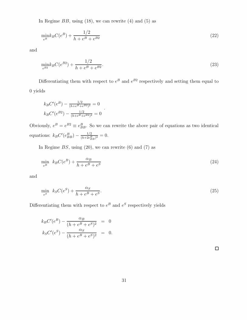
In Regime BB, using (18), we can rewrite (4) and (5) as

mineB

kBC(eB) +1/2

h+ eB + eB2(22)

and

mineB2

kBC(eB2) +1/2

h + eB + eB2. (23)

Differentiating them with respect to eB and eB2 respectively and setting them equal to

0 yields

kBC′(eB)− 1/2

(h+eB+eB2)2= 0

kBC′(eB2)− 1/2

(h+eB+eB2)2= 0

.

Obviously, eB = eB2 ≡ eBBB. So we can rewrite the above pair of equations as two identical

equations: kBC′(eBBB)− 1/2

(h+2eBBB)2= 0.

In Regime BS, using (20), we can rewrite (6) and (7) as

mineB

kBC(eB) +αB

h+ eB + eS(24)

and

mineS

kSC(eS) +αS

h + eB + eS. (25)

Differentiating them with respect to eB and eS respectively yields

kBC′(eB)− αB

(h+ eB + eS)2= 0

kSC′(eS)− αS

(h+ eB + eS)2= 0.

31

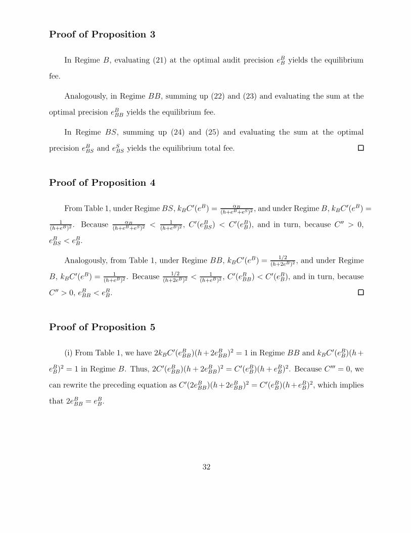
Proof of Proposition 3

In Regime B, evaluating (21) at the optimal audit precision eBB yields the equilibrium

fee.

Analogously, in Regime BB, summing up (22) and (23) and evaluating the sum at the

optimal precision eBBB yields the equilibrium fee.

In Regime BS, summing up (24) and (25) and evaluating the sum at the optimal

precision eBBS and eSBS yields the equilibrium total fee.

Proof of Proposition 4

From Table 1, under Regime BS, kBC′(eB) = αB

(h+eB+eS)2, and under RegimeB, kBC

′(eB) =

1(h+eB)2

. Because αB

(h+eB+eS)2< 1

(h+eB)2, C ′(eBBS) < C ′(eBB), and in turn, because C ′′ > 0,

eBBS < eBB.

Analogously, from Table 1, under Regime BB, kBC′(eB) = 1/2

(h+2eB)2, and under Regime

B, kBC′(eB) = 1

(h+eB)2. Because 1/2

(h+2eB)2< 1

(h+eB)2, C ′(eBBB) < C ′(eBB), and in turn, because

C ′′ > 0, eBBB < eBB.

Proof of Proposition 5

(i) From Table 1, we have 2kBC′(eBBB)(h+2eBBB)

2 = 1 in Regime BB and kBC′(eBB)(h+

eBB)2 = 1 in Regime B. Thus, 2C ′(eBBB)(h+ 2eBBB)

2 = C ′(eBB)(h+ eBB)2. Because C ′′′ = 0, we

can rewrite the preceding equation as C ′(2eBBB)(h+2eBBB)2 = C ′(eBB)(h+eBB)

2, which implies

that 2eBBB = eBB.

32

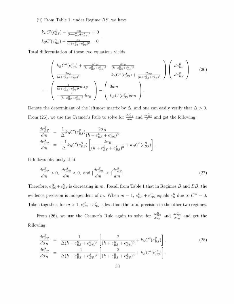
(ii) From Table 1, under Regime BS, we have

kBC′(eBBS)− αB

(h+eBBS+eSBS)2 = 0

kSC′(eSBS)− αS

(h+eBBS+eSBS)2 = 0

.

Total differentiation of those two equations yields⎛⎜⎝ kBC

′′(eBBS) +2αB

(h+eBBS+eSBS)3

2αB

(h+eBBS+eSBS)3

2αS

(h+eBBS+eSBS)3 kSC

′′(eSBS) +2αS

(h+eBBS+eSBS)3

⎞⎟⎠

⎛⎜⎝ deBBS

deSBS

⎞⎟⎠ (26)

=

⎛⎜⎝ 1

(h+eBBS+eSBS)2dαB

− 1(h+eBBS+eSBS)

2dαB

⎞⎟⎠−

⎛⎜⎝ 0dm

kBC′(eSBS)dm

⎞⎟⎠ .

Denote the determinant of the leftmost matrix by Δ, and one can easily verify that Δ > 0.

From (26), we use the Cramer’s Rule to solve fordeBBS

dmand

deSBS

dmand get the following:

deBBS

dm=

1

ΔkBC

′(eSBS)2αB

(h + eBBS + eSBS)3,

deSBS

dm=

−1

ΔkBC

′(eSBS)

[2αB

(h+ eBBS + eSBS)3+ kBC

′′(eBBS)

].

It follows obviously that

deBBS

dm> 0,

deSBS

dm< 0, and |de

BBS

dm| < |de

SBS

dm|. (27)

Therefore, eBBS+eSBS is decreasing in m. Recall from Table 1 that in Regimes B and BB, the

evidence precision is independent of m. When m = 1, eBBS + eSBS equals eBB due to C ′′′ = 0.

Taken together, for m > 1, eBBS+eSBS is less than the total precision in the other two regimes.

From (26), we use the Cramer’s Rule again to solve fordeBBS

dαBand

deSBS

dαBand get the

following:

deBBS

dαB=

1

Δ(h + eBBS + eSBS)2

[2

(h + eBBS + eSBS)3+ kSC

′′(eSBS)

], (28)

deSBS

dαB=

−1

Δ(h + eBBS + eSBS)2

[2

(h + eBBS + eSBS)3+ kBC

′′(eBBS)

].

33

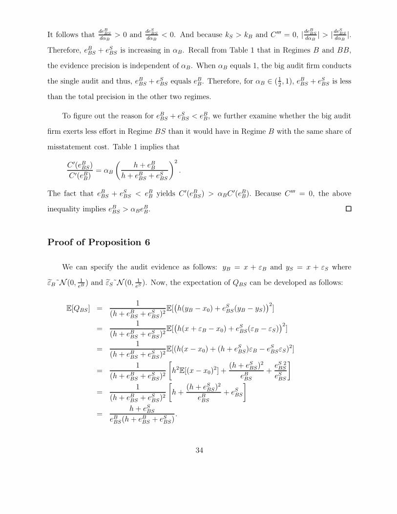
It follows thatdeBBS

dαB> 0 and

deSBS

dαB< 0. And because kS > kB and C ′′′ = 0, |deBBS

dαB| > |deSBS

dαB|.

Therefore, eBBS + eSBS is increasing in αB. Recall from Table 1 that in Regimes B and BB,

the evidence precision is independent of αB. When αB equals 1, the big audit firm conducts

the single audit and thus, eBBS + eSBS equals eBB. Therefore, for αB ∈ (12, 1), eBBS + eSBS is less

than the total precision in the other two regimes.

To figure out the reason for eBBS + eSBS < eBB, we further examine whether the big audit

firm exerts less effort in Regime BS than it would have in Regime B with the same share of

misstatement cost. Table 1 implies that

C ′(eBBS)

C ′(eBB)= αB

(h+ eBB

h+ eBBS + eSBS

)2

.

The fact that eBBS + eSBS < eBB yields C ′(eBBS) > αBC′(eBB). Because C ′′′ = 0, the above

inequality implies eBBS > αBeBB.

Proof of Proposition 6

We can specify the audit evidence as follows: yB = x + εB and yS = x + εS where

εB˜N (0, 1eB) and εS˜N (0, 1

eS). Now, the expectation of QBS can be developed as follows:

E[QBS ] =1

(h+ eBBS + eSBS)2E[(h(yB − x0) + eSBS(yB − yS)

)2]

=1

(h+ eBBS + eSBS)2E[(h(x+ εB − x0) + eSBS(εB − εS)

)2]

=1

(h+ eBBS + eSBS)2E[(h(x− x0) + (h+ eSBS)εB − eSBSεS)

2]

=1

(h+ eBBS + eSBS)2

[h2E[(x− x0)

2] +(h+ eSBS)

2

eBBS

+eS 2BS

eSBS

]

=1

(h+ eBBS + eSBS)2

[h+

(h + eSBS)2

eBBS

+ eSBS

]

=h+ eSBS

eBBS(h+ eBBS + eSBS).

34

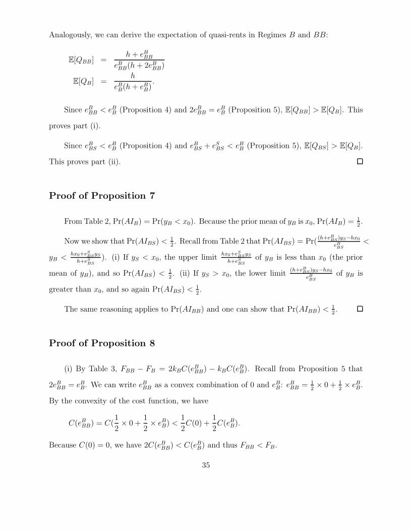
Analogously, we can derive the expectation of quasi-rents in Regimes B and BB:

E[QBB ] =h+ eBBB

eBBB(h + 2eBBB)

E[QB] =h

eBB(h+ eBB).

Since eBBB < eBB (Proposition 4) and 2eBBB = eBB (Proposition 5), E[QBB ] > E[QB ]. This

proves part (i).

Since eBBS < eBB (Proposition 4) and eBBS + eSBS < eBB (Proposition 5), E[QBS ] > E[QB].

This proves part (ii).

Proof of Proposition 7

From Table 2, Pr(AIB) = Pr(yB < x0). Because the prior mean of yB is x0, Pr(AIB) =12.

Now we show that Pr(AIBS) <12. Recall from Table 2 that Pr(AIBS) = Pr(

(h+eBBS)yS−hx0

eBBS<

yB <hx0+eSBSyS

h+eSBS). (i) If yS < x0, the upper limit

hx0+eSBSySh+eSBS

of yB is less than x0 (the prior

mean of yB), and so Pr(AIBS) < 12. (ii) If yS > x0, the lower limit

(h+eBBS)yS−hx0

eBBSof yB is

greater than x0, and so again Pr(AIBS) <12.

The same reasoning applies to Pr(AIBB) and one can show that Pr(AIBB) <12.

Proof of Proposition 8

(i) By Table 3, FBB − FB = 2kBC(eBBB) − kBC(eBB). Recall from Proposition 5 that

2eBBB = eBB. We can write eBBB as a convex combination of 0 and eBB: eBBB = 1

2× 0 + 1

2× eBB.

By the convexity of the cost function, we have

C(eBBB) = C(1

2× 0 +

1

2× eBB) <

1

2C(0) +

1

2C(eBB).

Because C(0) = 0, we have 2C(eBBB) < C(eBB) and thus FBB < FB.

35

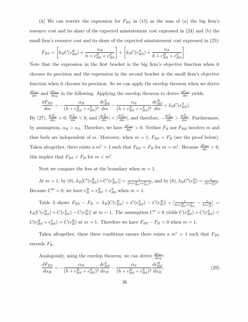
(ii) We can rewrite the expression for FBS in (15) as the sum of (a) the big firm’s

resource cost and its share of the expected misstatement cost expressed in (24) and (b) the

small firm’s resource cost and its share of the expected misstatement cost expressed in (25):

FBS =

[kBC(eBBS) +

αB

h + eBBS + eSBS

]+

[kSC(eSBS) +

αS

h+ eBBS + eSBS

].

Note that the expression in the first bracket is the big firm’s objective function when it

chooses its precision and the expression in the second bracket is the small firm’s objective

function when it chooses its precision. So we can apply the envelop theorem when we derive

dFBS

dmand dFBS

dαBin the following. Applying the envelop theorem to derive dFBS

dmyields

dFBS

dm= − αB

(h + eBBS + eSBS)2

deSBS

dm− αS

(h + eBBS + eSBS)2

deBBS

dm+ kBC(eSBS).

By (27),deBBS

dm> 0,

deSBS

dm< 0, and |deBBS

dm| < |deSBS

dm|, and therefore, −deSBS

dm>

deBBS

dm. Furthermore,

by assumption, αB > αS. Therefore, we havedFBS

dm> 0. Neither FB nor FBB involves m and

thus both are independent of m. Moreover, when m = 1, FBS < FB (see the proof below).

Taken altogether, there exists a m† > 1 such that FBS = FB for m = m†. Because dFBS

dm> 0,

this implies that FBS < FB for m < m†.

Next we compare the fees at the boundary when m = 1.

At m = 1, by (9), kB[C′(eBBS)+C ′(eSBS)] =

1(h+eBBS+eSBS)

2 , and by (8), kBC′(eBB) =

1(h+eBB)2

.

Because C ′′′ = 0, we have eBB = eBBS + eSBS when m = 1.

Table 3 shows FBS − FB = kB[C(eBBS) + C(eSBS) − C(eBB)] + [ 1h+eBBS+eSBS

− 1h+eBB

] =

kB[C(eBBS) +C(eSBS)−C(eBB)] at m = 1. The assumption C ′′ > 0 yields C(eBBS) +C(eSBS) <

C(eBBS + eSBS) = C(eBB) at m = 1. Therefore we have FBS − FB < 0 when m = 1.

Taken altogether, these three conditions ensure there exists a m† > 1 such that FBS

exceeds FB.

Analogously, using the envelop theorem, we can derive dFBS

dαB:

dFBS

dαB= − αB

(h + eBBS + eSBS)2

deSBS

dαB− αS

(h + eBBS + eSBS)2

deBBS

dαB. (29)

36

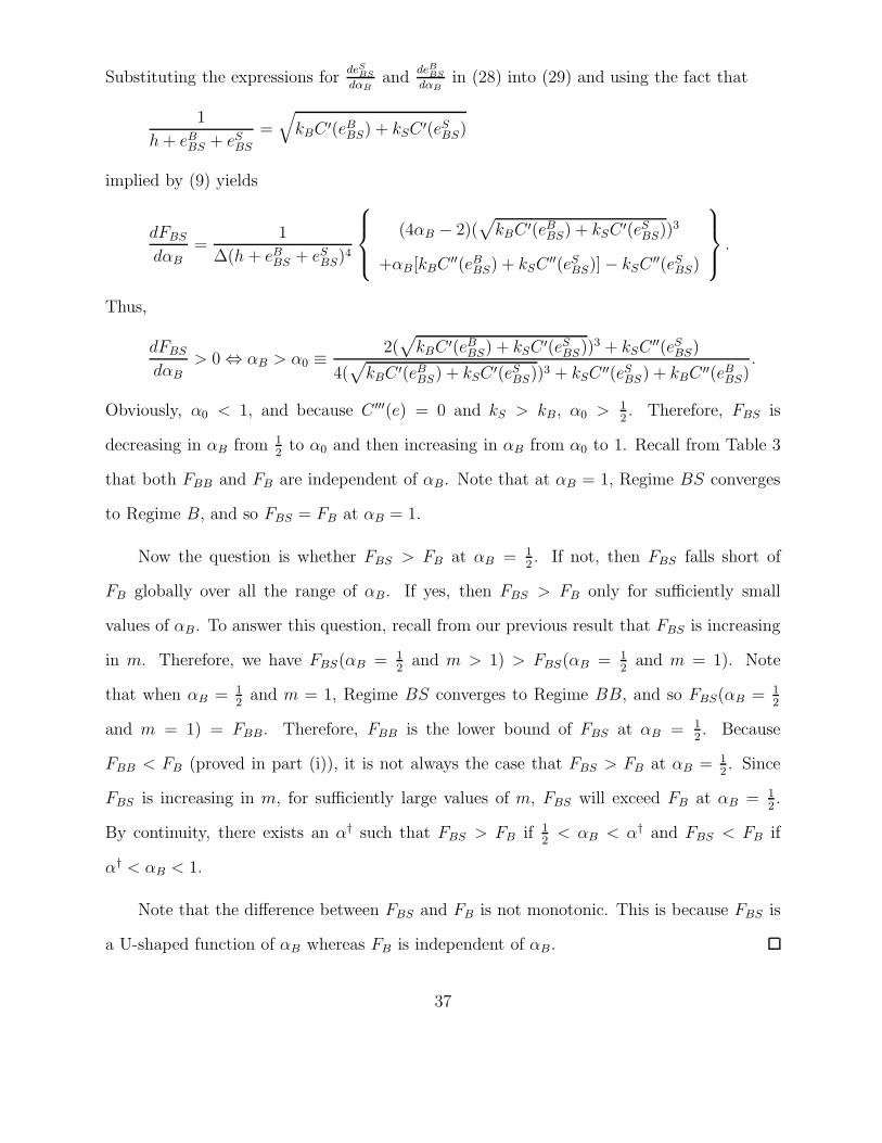
Substituting the expressions fordeSBS

dαBand

deBBS

dαBin (28) into (29) and using the fact that

1

h+ eBBS + eSBS

=√kBC ′(eBBS) + kSC ′(eSBS)

implied by (9) yields

dFBS

dαB

=1

Δ(h + eBBS + eSBS)4

⎧⎪⎨⎪⎩

(4αB − 2)(√kBC ′(eBBS) + kSC ′(eSBS))

3

+αB[kBC′′(eBBS) + kSC

′′(eSBS)]− kSC′′(eSBS)

⎫⎪⎬⎪⎭ .

Thus,

dFBS

dαB> 0 ⇔ αB > α0 ≡ 2(

√kBC ′(eBBS) + kSC ′(eSBS))

3 + kSC′′(eSBS)

4(√

kBC ′(eBBS) + kSC ′(eSBS))3 + kSC ′′(eSBS) + kBC ′′(eBBS)

.

Obviously, α0 < 1, and because C ′′′(e) = 0 and kS > kB, α0 > 12. Therefore, FBS is

decreasing in αB from 12to α0 and then increasing in αB from α0 to 1. Recall from Table 3

that both FBB and FB are independent of αB. Note that at αB = 1, Regime BS converges

to Regime B, and so FBS = FB at αB = 1.

Now the question is whether FBS > FB at αB = 12. If not, then FBS falls short of

FB globally over all the range of αB. If yes, then FBS > FB only for sufficiently small

values of αB. To answer this question, recall from our previous result that FBS is increasing

in m. Therefore, we have FBS(αB = 12and m > 1) > FBS(αB = 1

2and m = 1). Note

that when αB = 12and m = 1, Regime BS converges to Regime BB, and so FBS(αB = 1

2

and m = 1) = FBB. Therefore, FBB is the lower bound of FBS at αB = 12. Because

FBB < FB (proved in part (i)), it is not always the case that FBS > FB at αB = 12. Since

FBS is increasing in m, for sufficiently large values of m, FBS will exceed FB at αB = 12.

By continuity, there exists an α† such that FBS > FB if 12< αB < α† and FBS < FB if

α† < αB < 1.

Note that the difference between FBS and FB is not monotonic. This is because FBS is

a U-shaped function of αB whereas FB is independent of αB.

37

References

Antle, R. 1984. Auditor independence. Journal of Accounting Research 22 (1): 1–20.

Antle, R., and B. Nalebuff. 1991. Conservatism and auditor-client negotiations. Journal of

Accounting Research 29 (Supplement): 31–54.

Audousset-Coulier, S. 2012. “Two Big” or not “two Big”? The consequences of appointing

two Big 4 auditors on audit pricing in a joint audit setting. Working paper, JMSB -

Concordia University.

Chan, D. K., and S. Pae. 1998. An analysis of the economic consequences of the proportionate

liability rule. Contemporary Accounting Research 15 (4): 457–480.

DeAngelo, L. E. 1981a. Auditor independence, ‘low balling,’ and disclosure regulation.

Journal of Accounting and Economics 3 (2): 113–127.

DeAngelo, L. E. 1981b. Auditor size and audit quality. Journal of Accounting and Economics

3 (3): 183–199.

Dye, R. A. 1993. Auditing standards, legal liability, and auditor wealth. Journal of Political

Economy 101 (5): 887–914.

Dye, R. A., and S. S. Sridhar. 2004. Reliability-relevance tradeoffs and the efficiency of

aggregation. Journal of Accounting Research 42 (1): 51–88.

EC. 2010. Green paper - Audit policy: Lessons from the crisis. European Commission,

Brussels, October: 1–21.

Francis, J. R., C. Richard, and A. Vanstraelen. 2009. Assessing France’s joint audit require-

ment: Are two heads better than one? Auditing: A Journal of Practice and Theory 28

(2): 35–63.

38

Gonthier-Besacier, N., and A. Schatt. 2007. Determinants of audit fees for French quoted

firms. Managerial Auditing Journal 22 (2): 139–160.

Holm, C., and F. Thinggaard. 2010. Joint audits - Benefit or burden? Working paper,

University of Aarhus.

Kanodia, C., and A. Mukherji. 1994. Audit pricing, lowballing and auditor turnover: A

dynamic analysis. The Accounting Review 69(4): 593–615.

Laux, V., and P. Newman. 2010. Auditor liability and client acceptance decisions. The

Accounting Review 85 (1): 261–285.

Lesage, C., N. Ratzinger-Sakel, and J. Kettunen. 2011. Is joint audit bad or good? Efficiency

perspective evidence from three European countries. Working paper, HEC Paris, Ulm

University, and University of Jyvaskyla.

Lu, T. 2006. Does opinion shopping impair auditor independence and audit quality? Journal

of Accounting Research 44 (3): 561–583.

Magee, R. P., and M.-C. Tseng. 1990. Audit pricing and independence. The Accounting

Review 65 (2): 315–336.

Marmousez, S. 2008. The choice of joint-auditors and earnings quality: Evidence from

French listed companies. Working paper, HEC Montreal.

Pae, S., and S.-W. Yoo. 2001. Strategic interaction in auditing: An analysis of auditors’

legal liability, internal control system quality, and audit effort. The Accounting Review 76

(3): 333–356.

Paugam, L., and J. Casta. 2012. Joint audit, game theory, and impairment-testing disclo-

sures. Working paper, University Paris-Dauphine.

39

Piot, C. 2007. Auditor concentration in a joint-auditing environment: the French market

1997-2003. Managerial Auditing Journal 22 (2): 161–176.

Schwartz, R. 1997. Legal regimes, audit quality and investment. The Accounting Review 72

(3): 385–406.

Simunic, D. A. 1984. Auditing, consulting, and auditor independence. Journal of Accounting

Research 22 (2): 679–702.

Thinggaard, F., and L. Kiertzner. 2008. Determinants of audit fees: Evidence from a small

capital market with a joint audit requirement. International Journal of Auditing 12 (2):

141–158.

Zhang, P. 2007. The impact of the public’s expectations of auditors on audit quality and

auditing standards compliance. Contemporary Accounting Research 24 (2): 631–654.

40