Do Investors Overreact or Underreact to Accruals? A Reexamination of the Accrual Anomaly

Yong Yu* Smeal College of Business

Pennsylvania State University This draft: December 30, 2005

Abstract Sloan (1996) finds that the accrual component of earnings is negatively associated with subsequent stock returns. He interprets this negative association as evidence that investors fail to fully understand the lower persistence of accruals relative to cash flows and consequently overprice accruals. This observed overreaction to accruals has come to be known as the accrual anomaly. This paper reexamines the accrual anomaly, concentrating on how three different features of Sloan’s (1996) research design affect inferences regarding the existence of this anomaly, namely, the omission of cash flows, the use of an annual setting, and the reliance on the full sample of firms in examining investors’ reaction to accruals. The main findings of the paper are as follows: First, after controlling for cash flows and using a quarterly setting, accruals are found to be positively associated with subsequent returns, suggesting that investors underreact to accruals. This positive association is weaker than the positive association between cash flows and subsequent returns, suggesting that investors underreact to cash flows to a greater extent. Second, when cash flows are omitted, the more pronounced underreaction to cash flows than to accruals, combined with the negative correlation between accruals and cash flows, results in a severe downward bias on the association between accruals and subsequent returns. This bias conceals the underlying underreaction of investors to accruals, leading to the observed “accrual anomaly” reported by Sloan. These results hold for the full sample of firms on average and are even stronger for sub-samples of firms where accruals are likely to play a more important role in measuring firm performance. Finally, and in line with the above results, after a proper control for cash flows, financial analysts are found to underreact to accruals, in contrast to previous finding that analysts overreact to accruals.

*354 Business Building, Smeal College of Business, University Park, PA 16802. Email: yuy2@psu.edu Tel: (814)865-0601 This paper is based on my dissertation, undertaken at Pennsylvania State University. I appreciate the advice and suggestions of my dissertation committee: Orie Barron (co-chair), Dan Givoly (co-chair), Bin Ke, Jim McKeown, Karl Muller, and Mark Roberts. I thank Donal Byard, Paul Fisher, Carla Hayn, Steve Huddart, Andy Leone, Henock Louis, Shail Pandit, Santhosh Ramalingegowda, and Hal White for helpful comments.

1

1. Introduction

Sloan (1996) finds that the accrual component of earnings is negatively associated

with subsequent stock returns. He interprets this negative association as evidence that

investors fail to fully understand the lower persistence of accruals relative to cash flows

and consequently overprice accruals.1 Over the past decade, this observed overreaction to

accruals, which has been replicated by many studies, has come to be known as the

“accrual anomaly” and has generated interest among both researchers and investors.2

Studies on the accrual anomaly have taken different paths. One line of studies

investigates how the behavior of financial analysts, short sellers, and other third parties is

related to this anomaly (e.g., Bradshaw et al., 2001; Richardson, 2003). Another line

examines the role of different components of accruals in creating this anomaly (e.g., Xie,

2001; Thomas and Zhang, 2002; Richardson et al., 2005). A third line of research seeks

to relate this anomaly to other market anomalies (e.g., Collins and Hribar, 2000; Fairfield

et al., 2003; Desai et al., 2004). Some studies examine the relation of this anomaly to

various firm characteristics and risk measures (e.g., Ali et al., 2001; Mashruwala et al.,

2004; Khan, 2005). Other studies attempt to determine how widespread this anomaly is

(e.g., LaFond, 2005; Pincus et al., 2005).

In this study, I reexamine the accrual anomaly, concentrating on how three

different features of Sloan’s (1996) research design affect inferences regarding the

existence of this anomaly. The first feature is the omission of cash flows from the

1 Following Sloan (1996), the term overreaction (underreaction) is used to characterize a negative (positive) association between accruals or cash flows and subsequent returns. Accruals and cash flows refer to the accrual and cash flow components of earnings, and subsequent returns are the abnormal returns in the periods following the earnings report. 2 Following Sloan (1996), selling high-accrual firms’ stock and buying low-accrual firms’ stock has become a popular trading strategy (see, e.g., Talley, 2003; Henry, 2004a, 2004b). Reportedly, “now investors are clamoring to exploit this market inefficiency.” (Business Week, October 4, 2004, cover story)

2

examination of the association between accruals and subsequent returns. This omission is

problematic because cash flows are likely to be a significant correlated omitted variable.

More importantly, given a negative relation between accruals and cash flows and an

underreaction to cash flows, the omission of cash flows biases the results in favor of the

accrual anomaly. I analyze the impact of this correlated omitted variable problem and

examine whether, upon inclusion, the accrual anomaly still exists.

The second feature of Sloan’s (1996) research design is the use of an annual

setting whereby annual accruals and returns subsequent to the annual filing date are

examined. The use of this annual setting to detect investors’ reaction to accruals has two

limitations. First, annual accruals are likely to play a relatively minor role in correcting

cash flows as a measure of performance as compared to accruals for shorter measurement

intervals (e.g., quarters). This is the case because over longer measurement intervals, cash

flows suffer from fewer timing and matching problems, and the role of accruals

diminishes. Second, the returns over the period following the annual filing date do not

fully capture the potential mispricing of the first three quarters’ accruals. In this study, I

examine quarterly accruals and returns subsequent to the quarterly filing date.

The third feature of Sloan’s (1996) research design addressed in this study is the

reliance on the full sample of firms (i.e., all firms with data available) rather than on

firms where accruals are more important in measuring performance. For some firms, cash

flows and earnings are closely aligned; so any potential mispricing of accruals is likely to

have a relatively minor impact on stock returns than for other firms where accruals are

more informative. Conducting the analysis on the full sample of firms is therefore likely

to reduce the test’s power to detect investors’ reaction to accruals. In this study, I perform

3

tests on sub-samples of firms where accruals are likely to be more informative. Based on

prior research, these firms are identified as those with more volatile working capital

requirements and investment and financing activities and those with longer operating

cycles (Dechow, 1994; Dechow et al., 1998).

The main findings that emerge from the analyses are as follows. First, after

controlling for cash flows and using a quarterly setting, accruals are found to be

significantly positively associated with subsequent returns, suggesting that investors

underreact to accruals. This positive association is weaker than the positive association

between cash flows and subsequent returns, suggesting that while investors underreact to

accruals, they underreact to cash flows to a greater extent. Second, the results indicate

that when cash flows are omitted, the stronger underreaction to cash flows than to

accruals, combined with the negative correlation between accruals and cash flows, results

in a severe downward bias on the association between accruals and subsequent returns.

This bias conceals the underlying underreaction of investors to accruals, leading to the

observed “accrual anomaly” reported by Sloan. These results hold for the full sample of

firms on average and, as expected, are even stronger for sub-samples of firms where

accruals are likely to play a more important role in measuring firm performance.

To tie my results to past research on the manner by which analysts process the

accrual anomaly, I examine how financial analysts react to accruals using their forecasts

of future earnings. In line with my earlier results on the accrual anomaly, after a proper

control for cash flows, financial analysts are found to underreact to accruals and to

underreact even more to cash flows. Similarly, the results indicate that Bradshaw et al.’s

4

(2001) finding of analysts’ overreaction to accruals is driven by the omission of cash

flows from their analyses.

This study sheds light on an important topic of how investors and analysts react to

accruals. It shows that the observed “overreaction” to accruals by investors and analysts

(i.e., the accrual anomaly) is driven by a correlated omitted variable problem. Instead,

this study offers new evidence that investors and analysts underreact to accruals.

These findings have important implications for the accrual anomaly literature

which has largely focused on explaining why investors “overreact” to accruals. The

challenge now is to explain why investors underreact to accruals and why investors

underreact more to cash flows than to accruals. (Some possible explanations are

discussed in section 6.) 3 These results also help resolve a puzzling finding by previous

studies of an overreaction to one major component of earnings (accruals) and an

underreaction to the other major component of earnings (cash flows). 4

In section 2, I analyze the three features of Sloan’s research design that are likely

to bias his results. Data and variables used in the tests are discussed in section 3, and the

results of testing the association between accruals and subsequent stock returns are

presented in section 4. In section 5, I examine how financial analysts react to accruals

using their forecasts of future earnings. Section 6 contains conclusions and possible

explanations for the findings in this study.

3The findings in this study have implications for investors implementing the “accrual anomaly” strategy of selling high-accrual firms and buying low-accrual firms. Because the “overreaction” to accruals they attempt to exploit is shown to be only part of the underlying underreaction to cash flows, these investors could devise investment strategies superior to that relying on accruals. This can be accomplished by either directly focusing on the first order effect, cash flows (i.e., buying high-cash flow firms and selling low-cash flow firms), or using a combined strategy of buying firms with both high cash flows and high accruals and selling firms with both low cash flows and low accruals. 4 As noted by Kothari (2001), “one challenge is to understand why the market underreacts to earnings, but its reaction to its two components, cash flows and accruals, is conflicting.”

5

2. Features of Sloan’s (1996) Research Design

2.1 Omission of Cash Flows

Sloan (1996) omits cash flows in his examination of the association between

accruals and subsequent returns.5 This omission is problematic because cash flows are

likely to be a significant correlated omitted variable. To analyze this problem, consider

the following model which examines the association between the two earnings

components and subsequent returns (firm subscripts are omitted for brevity):

)1(12101 ++ +++= tttt �*CASHFLOWS�*ACCRUALS��RETURN

where 1+tRETURN = abnormal returns over period t+1;

tACCRUALS = scaled decile portfolio rank based on accruals in period t;

tCASHFLOWS = scaled decile portfolio rank based on cash flows in period t;

1+t� = an error term.

In Equation (1), the accrual (cash flow) decile ranks are scaled to [0,1] such that

firms with the most positive accruals (cash flows) have a portfolio rank of 1 and firms

with the most negative accruals (cash flows) have a rank of 0. Under this construction,

the coefficients can be interpreted as abnormal returns on portfolios with certain useful

properties (see, e.g., Fama and MacBeth, 1973; Bernard and Thomas, 1990). For

example, 1β ( )2β represents the abnormal returns earned by a zero-investment hedge

portfolio strategy of buying firms in the highest accrual (cash flow) decile and selling

firms in the lowest accrual (cash flow) decile. Note that the “accrual anomaly” strategy

5 Sloan (1996) does consider both cash flows and accruals in comparing a measure of investors’ pricing of accruals and cash flows with a measure of the implication of accruals and cash flows for one-year-ahead earnings (i.e., the Mishkin test) (see also Kraft et al., 2005a). However, it is important to note that Sloan omits cash flows in the examination of the association between accruals and subsequent returns.

6

would then earn an abnormal return of 1β− . Consistent with Sloan, a negative (positive)

coefficient is interpreted as an overreaction (underreaction), and the magnitude of the

coefficient indicates the economic magnitude of the overreaction (underreaction).

Sloan (1996) finds that a trading strategy of selling firms in the highest accrual

decile and buying firms in the lowest accrual decile earns significant subsequent

abnormal returns. This is equivalent to estimating Equation (1) excluding tCASHFLOWS

and finding that the estimated coefficient on tACCRUALS is significantly negative.

However, when tCASHFLOWS are omitted, the estimated coefficient on tACCRUALS ,

denoted ∧

1β , is a biased estimate of 1β .6 Specifically,

)2(*)(

),()( 211 βββ

t

tt

ACCRUALSVarCASHFLOWSACCRUALSCov

E +=∧

where ),( tt CASHFLOWSACCRUALSCov is the covariance between tACCRUALS and

tCASHFLOWS , and tACCRUALSVar( ) is the variance of tACCRUALS .

Since both tACCRUALS and tCASHFLOWS are decile portfolio ranks ranging

from [0,1], they have the same variance. Therefore, Equation (2) can be rewritten as:

)3(*),()( 211 βββ tt CASHFLOWSACCRUALSCorrE +=∧

where ),( tt CASHFLOWSACCRUALSCorr is the correlation between tACCRUALS and

tCASHFLOWS . Equation (3) shows that the bias in ∧

1β is determined by two factors: the

correlation between accruals and cash flows, and the mispricing of cash flows.7

6 See Wooldridge (2003, Chapter 3) and Greene (2003, Chapter 8). 7 Similar to the omission of cash flows in examining accruals and subsequent returns, Sloan (1996) also omits accruals in documenting a positive association between cash flows and subsequent returns. By examining both accruals and cash flows concurrently, this study also provides evidence that the omission of

7

The primary role of accruals in mitigating timing and matching problems inherent

in cash flows results in a negative correlation between the two earnings components.

Given an underreaction to cash flows (i.e., 02 >β ), the omission of cash flows causes a

downward bias in ∧

1β (i.e., )0*),( 2 <βtt CASHFLOWSACCRUALSCorr . Depending on

the severity of this downward bias, the observed “accrual anomaly” ( )01 <∧

β is consistent

with three potential explanations:

• Investors overreact to accruals (i.e., 01 <β ). The accrual anomaly indeed holds.

However, because its magnitude is overstated due to the downward bias, the

question remains as to whether or not the anomaly is economically significant.

• Investors price accruals correctly (i.e., 01 =β ). The observed “overreaction” to

accruals is driven by the downward bias, and there is no mispricing of accruals.

• Investors underreact to accruals (i.e., 01 >β ). There appears to be an “accrual

anomaly” because the downward bias dominates the positive coefficient ( 1β ).

Specifically, [ ] 12*),( ββ >− tt CASHFLOWSACCRUALSCorr . Because

[ ]),( tt CASHFLOWSACCRUALSCorr− is between 0 and 1, this suggests that

12 ββ > , that is, investors underreact to cash flows to a greater extent than they

underreact to accruals. In other words, the apparent “accrual anomaly” is driven

by the more severe underreaction to cash flows than to accruals, combined with

the negative correlation between accruals and cash flows.

accruals biases downward the association between cash flows and subsequent returns and thus understates investors’ underreaction to cash flows (see section 4 for the results).

8

To summarize, the above analysis shows that the omission of cash flows from

Sloan’s analysis leaves the existence of the accrual anomaly an open question. To address

this question, I examine the association between accruals and subsequent returns while

controlling for the effect of cash flows.8

2.2 Use of an Annual Setting

Sloan (1996) finds the accrual anomaly in tests using annual accruals and returns

subsequent to the annual filing date. The use of this annual setting to detect investors’

reaction to accruals has two limitations.

First, annual accruals play a lesser role in improving cash flows as a measure of

firm performance than accruals over shorter measurement intervals (e.g., quarters). The

accrual process is hypothesized to mitigate the timing and matching problems inherent in

cash flows over finite measurement intervals so that earnings better approximate firm

performance (e.g., Watts and Zimmerman, 1986; Dechow, 1994; Dechow et al., 1998).

Because cash flows suffer more severely from timing and matching problems and are

thus less informative about firm performance over shorter intervals, accruals over such

intervals are more important in providing value-relevant information about firm

performance. Over longer intervals, cash flows have fewer problems and converge to

earnings; so the role of accruals diminishes. This property of accruals suggests that

accruals over a quarterly interval provide a more powerful setting in which to examine

investors’ reaction to accrual information.

8 Desai et al. (2004) also incorporate cash flows in their test of the accrual anomaly. However, they are not interested in the functional relation between accruals and cash flows. Rather, they examine whether the accrual anomaly is subsumed by the “value-glamour” anomaly. Using cash flows to capture the value-glamour distinction in an annual setting, they find that when cash flows are added to accruals in the regression, the coefficient on accruals is negative but statistically insignificant. They conclude that the accrual anomaly is the value-glamour anomaly in disguise. I show that their finding of an insignificant negative relation between accruals and subsequent returns is due to their use of an annual setting.

9

The second limitation of using an annual setting is that it ignores accrual

information provided in interim reports. This information preempts at least part of the

accrual information released in annual reports. As a result, abnormal returns measured

over the period following the annual filing date reflect primarily the potential mispricing

of the fourth-quarter accruals and fail to fully capture the potential mispricing of the first

three quarters’ accruals. For example, consider the information conveyed by first-quarter

accruals. By the fourth month after fiscal year-end (when returns begin to be measured in

the tests using the annual setting), first-quarter accrual information has been released for

about one year; so only part, if any, of investors’ initial (anomalous) reaction to this

information is captured by the post-annual-report returns.

To overcome the two limitations arising from the use of the annual setting, I

examine investors’ reaction to accruals in a quarterly setting using quarterly accruals and

returns subsequent to the quarterly filing date.

2.3 Reliance on the Full Sample of Firms

In documenting the accrual anomaly, Sloan (1996) conducts tests on the entire

sample of firms (i.e., all firms with data available). However, the importance of accruals

in measuring firm performance is likely to vary across firms. For some firms, cash flows

suffer from more timing and matching problems than for other firms, and therefore their

accruals play a more important role in measuring performance. If investors misprice

accruals, this mispricing will be more pronounced (i.e., have a relatively larger impact on

stock returns) for these firms. However, for some other firms, cash flows have fewer

problems in measuring performance and are closely aligned with earnings; so the role of

accruals diminishes. For these firms, the mispricing of accruals, if any, is likely to have a

10

relatively minor impact on stock returns and harder to detect statistically. The inclusion

of these firms in the tests reduces the power to detect investors’ reaction to accruals.

In this study, I examine sub-samples of firms where accruals are likely to play a

more important role in measuring firm performance. These firms are identified as those

with more volatile working capital requirements and investment and financing activities

and those with longer operating cycles. Prior research documents that for these firms,

cash flows suffer from more timing and matching problems and accruals are therefore

more important in measuring performance (Dechow, 1994; Dechow et al., 1998).

To summarize, I reexamine the accrual anomaly, modifying the research design of

Sloan (1996) by controlling for cash flows, using a quarterly setting, and partitioning the

sample according to the importance of accruals in mitigating the problems of cash flows

as a measure of performance. In the following two sections, I first examine the

association between annual accruals and returns subsequent to the annual filing date

using the full sample of firms (hereafter, the annual test) to facilitate a comparison with

prior research. I then conduct the main analysis in a quarterly setting, examining

quarterly accruals and returns subsequent to the quarterly filing date. This analysis is

performed on the full sample first (hereafter, the quarterly test) and then on sub-samples

of firms where accruals play a more important role (hereafter, the sub-sample test).

3. Sample Selection and Variable Measurement

3.1 Sample Selection

The sample used in the annual (quarterly) test consists of all available

NYSE/AMEX firm-years (firm-quarters) from 1988 through 2002 with required financial

11

statement data on the Compustat database and monthly return data on the CRSP

database.9 In order to ensure that cash flows and accruals are accurately measured, the

sample period begins in 1988 when cash flow statement data became available.10

Following prior research, I exclude closed-end funds, investment trusts, foreign

companies, and financial institutions (SIC code 6000-6999) due to the difficulty of

interpreting accruals for financial firms.11 This results in a sample of 25,540 firm-years

for the annual test and a sample of 79,809 firm-quarters for the quarterly test, spanning a

sixty-quarter period from 1988 through 2002.

3.2 Variable Measurement

Accruals are measured as the difference between earnings and cash flows from

operations taken from the statement of cash flows. Earnings are income from continuing

operations, and cash flows are cash flows from continuing operations. All three variables

are scaled by average total assets.12

The abnormal return measure is the annual size-adjusted buy-and-hold returns as

used in Sloan (1996). Raw returns are obtained from the CRSP monthly return file.

Abnormal returns are computed by subtracting a firm’s size-matched buy-and-hold

returns from the raw buy-and-hold returns. Size portfolio returns are provided by CRSP

9 NYSE/AMEX firms are identified using the historical exchange code (EXCHCD) from the CRSP monthly event file in the month before the return calculation. Using current exchange listing (e.g., Compustat’s Zlist or CRSP’s header exchange code) introduces a selection bias because changes in exchange listing are correlated with firm performance and a firm currently on the NYSE/AMEX may be traded on other exchanges in the past. Using EXCHCD avoids this selection bias (Kraft et al., 2005b). 10 Sloan (1996) uses a balance sheet approach to measure accruals. This approach introduces measurement errors into the accruals measure, particularly when a firm has been involved in mergers, acquisitions, or divestitures. Measuring accruals using cash flows statement data is more precise (see, e.g., Drtina and Largay, 1985; Hribar and Collins, 2002). 11 The results are similar if these observations are included. 12 For the annual sample, earnings are Compustat Annual Item 123, cash flows are Compustat Annual (Item 308 – Item 124), and total assets are Compustat Annual Item 6. For the quarterly sample, earnings are Compustat Quarterly Item 76, cash flows are Compustat Quarterly (Item 108 – Item 78), and total assets are Compustat Quarterly Item 44. Note that for quarterly cash flow statement items, Compustat reports data for the cumulative interim period year to date.

12

and calculated using all NYSE/AMEX firms based on their beginning-of-year market

capitalizations. A firm’s return is set to zero for any month if it is missing due to lack of

trading.13 If a firm is delisted during the return accumulation period, the delisting return

as reported in the CRSP event file for the delisting period is used, and a return equal to

the firm’s size portfolio return for the rest of the accumulation period is employed. If a

firm is delisted due to liquidation or a forced delisting by either the exchange or the SEC

and the delisting return is missing, the delisting return is set to -100%.14

Following Sloan (1996), the future buy-and-hold abnormal returns in the annual

test, denoted ANNBHAR , are measured from four months after the fiscal year-end through

the fourth month of the subsequent fiscal year. Similarly, the future buy-and-hold

abnormal returns in the quarterly test, denoted QTRBHAR , span the twelve-month period

beginning two months after the fiscal quarter-end for the first three fiscal quarters and

four months after the fiscal quarter-end for the fourth fiscal quarter.15 Within this two-

month interval, almost all firms have filed 10-Q reports for the first three fiscal quarters,

and within the four-month interval, almost all firms have filed 10-K reports (Easton and

Zmijewski, 1993).

13 This is identified using CRSP code “.B” in the return field. Excluding firms with missing returns due to a lack of trading activity disproportionately affects firms with bad stock performance, and thus excluding their returns imposes an upward bias in measuring abnormal returns (Kraft et al., 2005b). Nevertheless, the results are robust to excluding these observations or replacing these missing returns with the corresponding size decile returns. 14 The results remain unchanged if I delete these delisting firms or assume a delisting return of zero. 15 I repeat the analyses using 3- and 6-month windows. The results using these shorter return windows are stronger (see Section 4.5 for a discussion and results).

13

4. Results of Examining the Association between Accruals and Subsequent Returns

4.1 Descriptive Statistics and Correlations

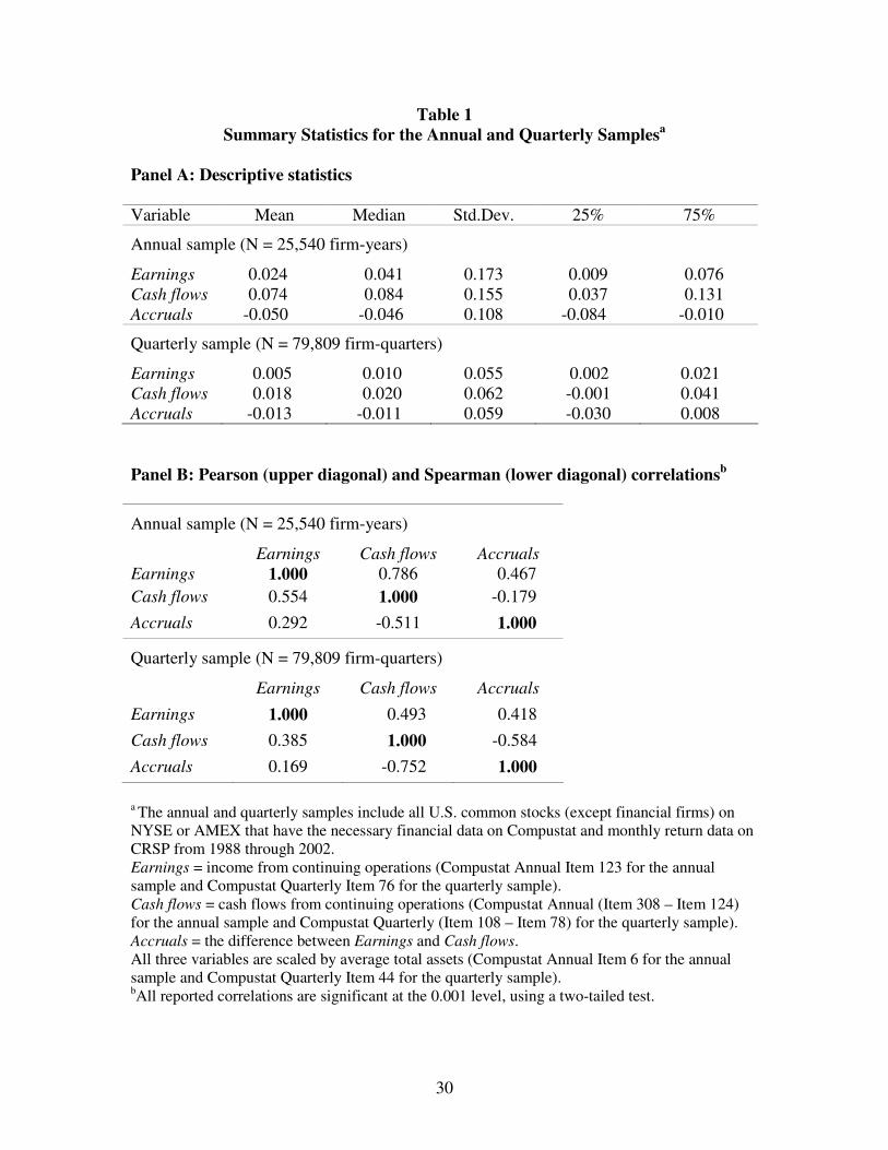
Table 1 provides descriptive statistics (Panel A) and a correlation analysis (Panel

B) for both the annual and quarterly samples. Panel A indicates that on average accruals

are negative and cash flows are positive. Panel B shows that accruals are highly

negatively correlated with cash flows, consistent with the primary role of accruals in

mitigating the timing and matching problems inherent in cash flows. Moreover, the

magnitude of the negative correlation between cash flows and accruals is larger in the

quarterly sample (Spearman = -0.752) than in the annual sample (Spearman = -0.511),

consistent with cash flows suffering more severely from timing and matching problems

and accruals playing a more important role in mitigating these problems over shorter

performance measurement intervals (Dechow, 1994).

4.2 Annual Test

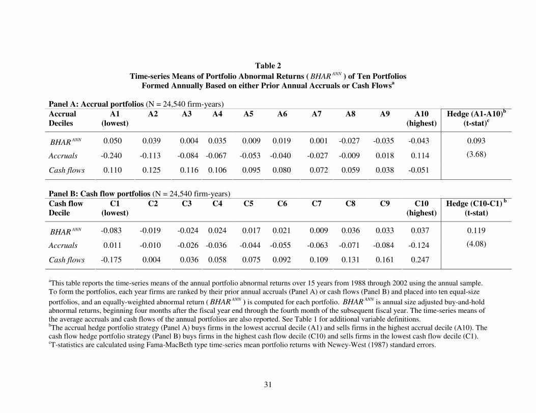
Table 2, Panel A replicates the accrual anomaly using the annual sample. To

conduct this analysis, each year firms are ranked by their prior annual accruals and placed

into ten equal-size portfolios, denoted A1 to A10. An equally-weighted abnormal return

is computed for each portfolio. The reported t-statistics are calculated using the Fama-

MacBeth (1973) method and corrected for auto-correlation using Newey and West (1987)

standard errors. Panel A presents the average portfolio returns, accruals, and cash flows

over fifteen years for each of the ten accrual portfolios.

The results are consistent with the accrual anomaly: a hedge portfolio strategy of

selling the most positive accrual firms (portfolio A10) and buying the most negative

accrual firms (portfolio A1) yields an annual abnormal return of 9.3%. On the other hand,

14

given the strong negative correlation between accruals and cash flows, it is not surprising

to find that firms in the most positive (negative) accrual portfolio also have extremely

negative (positive) cash flows. Because this univariate analysis does not control for the

effect of cash flows, the negative association between accruals and subsequent returns

cannot be unambiguously interpreted as evidence that investors overreact to accruals.

Panel B repeats the above analysis on cash flows. The results indicate that a strategy of

selling the most negative cash flow firms (portfolio C1) and buying the most positive

cash flow firms (portfolio C10) yields an annual abnormal return of 11.9%.

To control for the effect of cash flows, I regress subsequent returns on the scaled

accrual decile ranks (ACCRUALS) and the scaled cash flow decile ranks (CASHFLOWS).

The scaled decile ranks are constructed by ranking all firms in each period independently

on accruals and cash flows into deciles 0-9 and then dividing the decile ranks by 9 so that

they range from 0 (for the lowest decile) to 1 (for the highest decile).

Under this construction, the coefficient on ACCRUALS can be interpreted as the

abnormal returns to a zero-investment trading strategy of buying firms in the highest

accrual decile and selling firms in the lowest accrual decile (Bernard and Thomas, 1990).

The coefficient on CASHFLOWS can be interpreted similarly. To ensure that the results

are not merely driven by the size or market-to-book effects, the scaled decile ranks for

size (SIZE) and market-to-book ratios (MB), constructed in a similar way, are included as

additional controls (see Kothari, 2001, for a discussion).16

16 Size is included as an additional control because size-adjusted returns may not fully control for the size effect (Bernard, 1987). The results are similar if these controls are not included. The results are robust to controlling for the market beta calculated using the prior 60-month return period. Note that controlling for the momentum factor is inappropriate because the underreaction to accruals and cash flows examined in this study is a momentum (drift) phenomenon.

15

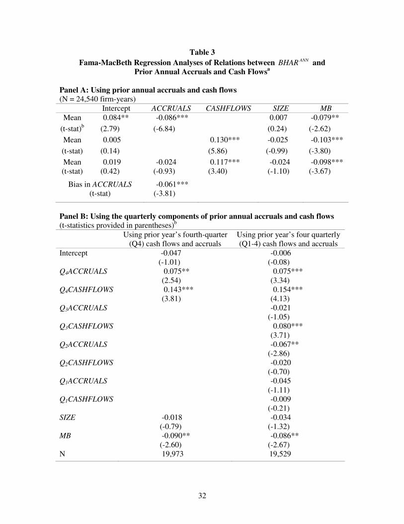
Table 3, Panel A reports Fama-MacBeth mean coefficient estimates from annual

regressions of ANNBHAR on the scaled decile ranks based on prior annual accruals

(ACCRUALS) and cash flows (CASHFLOWS). The coefficient on ACCRUALS, before

controlling for cash flows, is -0.086 (significant at the 0.01 level), consistent with the

accrual anomaly. However, after controlling for cash flows, the coefficient on

ACCRUALS decreases to -0.024 and becomes statistically insignificant (t-stat = -0.93).17

The omission of cash flows causes a downward bias of -0.061 (significant at the 0.01

level) in the coefficient on ACCRUALS.18 This insignificant relation between accruals

and subsequent returns after controlling for cash flows is consistent with two potential

explanations: (1) investors price accruals correctly, or (2) the annual test has limited

ability to detect the mispricing of accruals.

The analyses in Panel A constrain the coefficients on the quarterly components of

annual accruals to be equal. As discussed in section 2.2, one problem that arises with the

use of this annual setting is that the dependent variable, ANNBHAR , reflects primarily the

potential mispricing of the fourth-quarter accruals and fails to fully capture the potential

mispricing of the first three quarters’ accruals. In Table 3, Panel B, I allow the coefficient

to vary across the quarterly components of annual accruals and focus on the association

between ANNBHAR and the fourth-quarter accruals. Column 1 reports the mean coefficient

estimates from annual regressions of ANNBHAR on the scaled decile ranks based on the 17 Untabulated analyses indicate that this result is sensitive to some possible outliers. After deleting 1% of the annual sample with the largest squared residuals (Knez and Ready, 1997), I find that the coefficient on ACCRUALS is 0.048 (t-stat = 2.81) after controlling for cash flows. 18 To assess potential multicollinearity for the regression analyses including both accruals and cash flows, I compute the variance-inflation factor (VIF) for all the regressions. A general rule of thumb is that a VIF less than 20 does not indicate severe multicollinearity. Untabulated results show that no variable in any regression has a VIF more than 10 (e.g., in the 60 quarterly regressions including both accruals and cash flows as reported in Table 5, the median (maximum) VIF for ACCRUALS and CASHFLOWS is 2.43 (5.41) and 2.58 (5.66) respectively), indicating multicollinearity is not a problem. (For a discussion about multicollinearity, see Maddala, 2001, and Greene, 2003).

16

prior year’s fourth-quarter accruals (Q4ACCRUALS) and cash flows (Q4CASHFLOWS).

The sample consists of all the firm-years in the annual sample with the required fourth-

quarter data for that firm-year. The coefficient on Q4ACCRUALS (after controlling

Q4CASHFLOWS) is 0.075 (significant at the 0.05 level). The coefficient on

Q4CASHFLOWS is also significantly positive (0.143, significant at the 0.01 level) and

almost twice as large as the coefficient on Q4ACCRUALS. In Column 2, I repeat the

analyses in Column 1 but control for the first three quarters’ accruals and cash flows. The

results are very similar: the coefficient on Q4ACCRUALS is significantly positive (0.075,

significant at the 0.01 level), and the coefficient on Q4CASHFLOWS is twice as large as

the coefficient on Q4ACCRUALS (0.154, significant at the 0.01 level).19

The results in Panel B suggest that the insignificant relation between annual

accruals and subsequent returns in Panel A is likely driven by the limited ability of the

annual test to detect investors’ reaction to accruals. Allowing coefficients to vary across

the quarterly components of annual accruals gives evidence consistent with investors

underreacting to accruals (see Panel B).

4.3 Quarterly Test

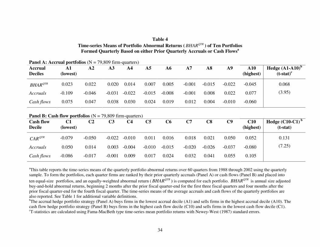
Table 4 replicates the accrual anomaly using the quarterly sample. To conduct this

analysis, ten equal-sized portfolios are formed each quarter based on prior quarterly

accruals, and an equally-weighted abnormal return ( QTRBHAR ) is then computed for each

portfolio. T-statistics are calculated using Fama-MacBeth type time-series mean portfolio

returns with Newey-West (1987) standard errors. Panel A of Table 4 reports the average

portfolio return and accruals and cash flows over sixty quarters for each of the ten

19 The coefficients on QiACCRUALS (i = 1,2,3) are generally not significant except Q2ACCRUAL (-0.067, t-stat = -2.86). Further analyses indicate that this is caused by a few extreme observations. After deleting 1% of the sample with the largest squared residuals, this coefficient becomes -0.023 (t-stat = -0.88).

17

portfolios. The results are consistent with the accrual anomaly: a trading strategy of

selling the most positive accrual firms and buying the most negative accrual firms yields

a significant annual abnormal return of 6.8%. Panel B indicates that a trading strategy of

selling firms with the most negative cash flow and buying firms with the most positive

cash flow yields an even greater abnormal return, 13.1% per year.

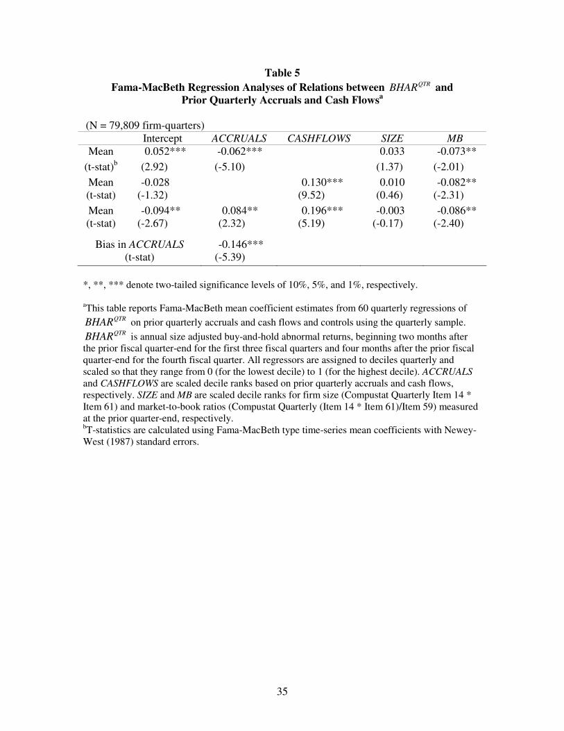
Table 5 reports Fama-MacBeth mean coefficient estimates from quarterly

regression analyses of QTRBHAR on the scaled decile ranks based on prior quarterly

accrual (ACCRUALS) and cash flow (CASHFLOWS). When cash flows are omitted, the

coefficient on ACCRUALS is -0.062 (significant at the 0.01 level), consistent with the

accrual anomaly. However, the sign of the coefficient on ACCRUALS, after controlling

for cash flows, becomes positive, and this positive coefficient is both economically and

statistically significant (0.084, significant at the 0.05 level). Thus, when cash flows are

omitted, the omission of cash flows causes a downward bias (-0.146, significant at the

0.01 level) in the coefficient on ACCRUALS. This bias is so severe that it dominates the

underlying positive relation between accruals and subsequent returns.

Similarly, the results indicate that the omission of accruals also biases downward

(but does not dominate) the association between cash flows and subsequent returns.

Specifically, the coefficient on CASHFLOWS is 0.196 when accruals are controlled for,

but is reduced to 0.130 by the omission of accruals.

The relative magnitude of the coefficients on ACCRUALS and CASHFLOWS is

noteworthy. When both are included in the regression, the positive coefficient on

CASHFLOWS is more than twice as large as the positive coefficient on ACCRUALS, with

the difference of 0.112 between the two coefficients (significant at the 0.01 level). This

18

large difference between the two coefficients explains why the omission of cash flows

not only biases downward the coefficient on accruals but turns it negative and significant

(see section 2.1).20

These results suggest: (1) investors underreact to accruals; (2) while underreacting

to accruals, investors underreact even more to cash flows; and (3) when cash flows are

omitted from the analysis, the stronger underreaction to cash flows than to accruals,

combined with the negative correlation between the two, imposes a downward bias on the

association between accruals and subsequent returns. This bias dominates the underlying

underreaction to accruals, leading to the observed “accrual anomaly.”21

4.4 Sub-sample Test

The sub-sample test, like the quarterly test above, also examines quarterly

accruals and returns subsequent to the quarterly filing date. However, instead of using the

full sample of firms, the sub-sample test examines sub-samples of firms where cash flows

are likely to suffer from more timing and matching problems and where accruals

therefore play a more important role in measuring firm performance. Based on prior

research, these firms are identified as those with more volatile working capital

requirements and investment and financing activities and those with longer operating

cycles. Because examining these firms provides a relatively more powerful test of

investors’ reaction to accruals than examining all firms, I expect to find even stronger

evidence of investors’ underreacting to accruals in this sub-sample test.

20 To ensure that the results are not driven by particular fiscal quarters, I repeat the analyses separately for each fiscal quarter and find that the results for the whole sample hold for each fiscal-quarter sample. 21 Xie (2001) finds that the negative association between accruals and subsequent returns is primarily attributable to abnormal accruals calculated from the Jones model. This finding is not surprising given that the negative correlation between accruals and cash flows is primarily attributable to the abnormal accruals (see, e.g., Xie, 2001, Table 1). Therefore, the downward bias caused by the omission of cash flows is expected to be largely captured by the abnormal accruals. The untabulated results indicate this is the case.

19

Following Dechow (1994), the volatility of working capital requirements and

investment and financing activities is measured by the absolute magnitude of accruals,

and the length of operating cycles is measured each quarter as follows:

)5(90/

2/)(90/

2/)( 11���

����

� ++��

���

� += −−

SOLDGOODSofCOSTINVINV

SALESARAR

cycleOperating tttt

where AR is accounts receivable (Compustat Quarterly Item 37), INV is inventory

(Compustat Quarterly Item 38), SALES are net sales (Compustat Quarterly Item 2), and

COST of GOODS SOLD is cost of good sold (Compustat Quarterly Item 30). In Equation

(5), the first component captures the speed of converting credit sales into cash, and the

second measures the number of days it takes to produce and sell products.22

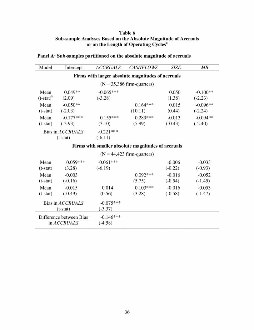
Table 6, Panel A reports the results for sub-samples partitioned based on the

absolute magnitude of accruals (a measure of the volatility of working capital

requirements and investment and financing activities). The quarterly sample is partitioned

into two sub-samples with an equal number of firms based on firms’ median absolute

magnitudes of quarterly accruals. The same analysis as in Table 5 is performed separately

for the two sub-samples. Compared with the results based on the full quarterly sample

(see Table 5), the test based on a sub-sample of firms with larger magnitudes of accruals

yields stronger evidence of investors underreacting to accruals. For this sub-sample of

firms, the coefficient on ACCRUALS, after controlling for cash flows, is 0.155

(significant at the 0.01 level), and much larger compared with that for the full sample

22 I also use a second measure proposed by Dechow (1994) for the length of operating cycles, which is calculated as:

��

���

� +−���

����

� ++��

���

� += −−−

90/2/)(

90/2/)(

90/2/)( 111

PURCHASESAPAP

SOLDGOODSofCOSTINVINV

SALESARAR

cycleTrade tttttt

where AP is accounts payable. The results using this second measure are similar to those using the first measure.

20

(0.084, Table 5). For other firms with smaller magnitudes of accruals, the coefficient on

ACCRUALS, after controlling for cash flows, is only weakly positive and statistically

insignificant (0.014, t-stat = 0.56). In addition, when cash flows are omitted, the

downward bias in the coefficient on ACCRUALS is more severe for firms with larger

magnitudes of accruals (-0.221) than for other firms (-0.075).

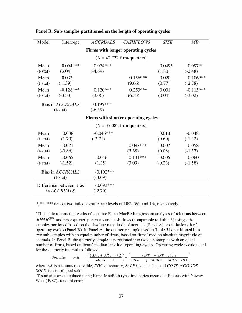
Table 6, Panel B reports the results for sub-samples partitioned based on the

length of operating cycles. For each firm-quarter, an operating cycle is computed using

Equation (5). A firm-specific operating cycle is calculated as the median of all the

computed operating cycles for this firm. The quarterly sample is then partitioned into two

sub-samples with an equal number of firms based on firm-specific operating cycles. The

analyses are conducted separately for the two sub-samples. As expected, the test using

firms with longer operating cycles provides stronger evidence of an underreaction of

investors to accruals. For firms with longer operating cycles, the coefficient on

ACCRUALS, after cash flows are controlled for, is 0.120 (significant at the 0.01 level),

compared with 0.084 for the full sample (Table 5) and 0.056 for firms with shorter

operating cycles. Also, the downward bias in the coefficient on ACCRUALS caused by

the omission of cash flows is more severe for firms with longer operating cycles (-0.195)

than for firms with shorter operating cycles (-0.102).

4.5 Additional Analyses

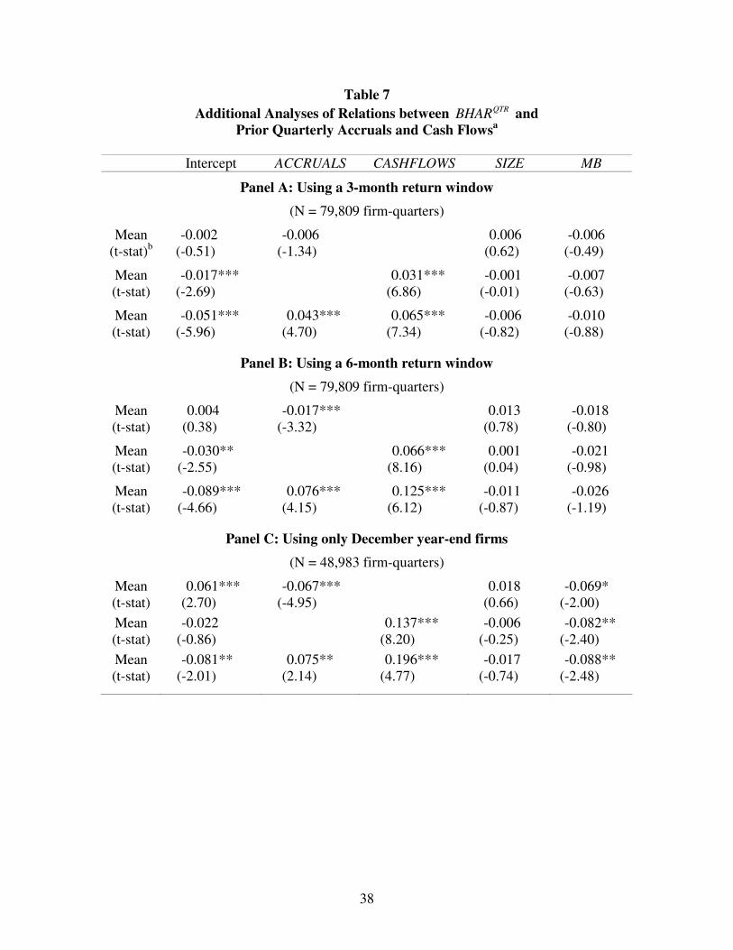
Shorter return windows

The analyses so far have used a 12-month return window, in line with Sloan

(1996). However, previous studies show that most of the market’s delayed response

(drift) occurs in the subsequent 3 to 6-month period (see, e.g., Bernard and Thomas,

21

1989; Jegadeesh and Titman, 1993), suggesting that tests using a shorter return window

are relatively more powerful. I repeat the analyses using 3- and 6-month return windows.

Panel A and B of Table 7 report the results of repeating the analyses in Table 5 using a 3-

month window and a 6-month window respectively. As expected, the results for these

shorter windows show stronger evidence of an underreaction of investors to accruals.

December year-end firms

The analyses so far have used firms with all fiscal year-ends to maximize sample

size. One potential concern is that the portfolio assignment is based on the distribution for

all firms in each period, including some that have not yet reported their accruals for that

period. If the distribution of accruals varies systematically with fiscal year-end, this may

cause a hindsight problem. I repeat the analyses using only December year-end firms and

find that my inferences remain unaltered (see Panel C of Table 7).

Influential observations

To ensure that the results are not driven by a small number of influential

observations, I repeat the analyses after excluding 1% of observations with the largest

squared residuals (Knez and Ready, 1997) and find that my inferences remain unchanged

(see Panel D of Table 7).

Small and illiquid firms

To investigate whether the results are primarily driven by small, illiquid firms, I

repeat the analyses after excluding all firms with stock prices lower than $5, and all firms

with a market capitalization that would put them into the smallest NYSE/AMEX size

decile (Jegadeesh and Titman, 2001). I find that my inferences remain unchanged after

excluding these small, illiquid stocks (see Panel E of Table 7).

22

5. Tests of Analysts’ Earnings Forecasts

In this section, I investigate financial analysts’ reaction to accruals through the

examination of the relation between accruals and their forecasts of future earnings. To the

extent that analysts’ forecasts of future earnings can be used as a proxy for investors’

expectations (e.g., Brown and Rozeff, 1978; Fried and Givoly, 1982; O’Brien, 1988), this

analysis provides me a setting to directly examine the link between accruals and

investors’ expectations of future firm performance. Since this analysis does not rely on

stock prices, it helps mitigate some of the concerns that unknown risk factors or research

design flaws may confound the return-based tests reported in Section 4.

Bradshaw et al. (2001) also investigate how analysts react to accruals. They find a

negative association between accruals and errors in analysts’ forecasts of future earnings

(defined as actual earnings minus forecast earnings). They interpret this negative

association as evidence that financial analysts, like investors, also overreact to accruals.

They conclude that this evidence confirms and complements the accrual anomaly

reported by Sloan (1996). However, Bradshaw et al. (2001) omit cash flows in their

examination of the association between accruals and analyst forecasts. So their result is

potentially biased by a similar correlated omitted variable problem that affects the

inferences concerning the accrual anomaly.

To assess the presence and extent of such a bias, I examine the association

between accruals and analysts’ forecast errors while controlling for the effect of cash

flows. Specially, I estimate the following model:

)6(12101 ++ +∗+∗+= tttt CASHFLOWSACCRUALSFERROR υααα

23

where 1+tFERROR is forecast errors for earnings in period t+1, tACCRUALS is accruals

in period t, and tCASHFLOWS is cash flows in period t. If analysts incorporate the

information in accruals efficiently, there should be no relation between accruals and

forecast errors. Otherwise, consistent with Bradshaw et al. (2001), a negative (positive)

coefficient on accruals is interpreted as an overreaction (underreaction) to accruals by

financial analysts. A similar interpretation applies to cash flows.

The sample used for estimating Equation (6) consists of all the observations in

the quarterly sample for which analysts’ median consensus forecasts and IBES actual

earnings are available on the IBES summary statistics file. Following Bradshaw et al.

(2001), the equation is estimated for each fiscal month from the month following quarter

t earnings announcement through the month before quarter t+1 earnings announcement.

Specifically, I initially measure the forecast for quarter t+1 earnings in the first month

after the quarter t’s earnings announcement and then track forecast errors over the months

leading up to the quarter t+1’s earnings announcement. I use Month 1, Month 2, and

Month 3 to denote the first, second, and third month after the quarter t announcement but

before the quarter t+1 announcement. Forecast errors are calculated as the difference

between IBES realized earnings and analysts’ median consensus forecasts, scaled by the

stock price at the end of quarter t. There are 53,923, 52,316 and 42,327 observations in

the samples for Month 1, 2, and 3 respectively.

Table 8 reports the summary statistics of the three monthly samples. The mean

forecasts suggest that analysts are optimistic. This optimism declines from Month 1 to

Month 3. The median forecast, however, does not show any obvious optimism or

pessimism. These patterns are consistent with prior findings (e.g., O’Brien, 1988;

24

Abarbanell and Lehavy, 2003). For all three samples, the Spearman correlation between

accruals and forecast errors is consistently negative and significant, while the Spearman

correlation between cash flows and forecast errors is consistently positive and significant.

Table 9 reports the results from estimating Equation (6). To mitigate the influence

of potential outliers caused by data error or extreme forecast errors (e.g., Abarbanell and

Lehavy, 2003; Gu and Wu, 2003), I perform a rank regression analysis using scaled

decile ranks for all the variables.23 Forecast errors, accruals, and cash flows are assigned

into deciles each quarter, and the quarterly decile ranks are scaled to the range [0,1] as

before. A separate estimation of Equation (6) is performed for each quarter, and the mean

coefficients, Fama-MacBeth t-statistics with Newey-West standard errors, and average R-

squares for the 60 quarterly estimations are reported in Table 9.

The tests on the three monthly samples (Month 1, 2, and 3) generate similar

findings. Specifically, when the effect of cash flows is controlled for, the association

between accruals and forecast errors is positive and significant. This positive association

is significantly smaller than the positive association between cash flows and forecast

errors. When cash flows are omitted, the association between accruals and forecast errors

is biased downward to such an extent that this association becomes negative and

significant, consistent with Bradshaw et al. (2001).

These results complement and reinforce the evidence concerning investors’

reaction to accruals reported in Section 4. The results suggest: (1) financial analysts

underreact to accruals; (2) analysts underreact to cash flows to a greater extent; and (3)

when cash flows are omitted, the stronger underreaction to cash flows than to accruals,

combined with the negative correlation between accruals and cash flows, produces a 23 The inferences are unchanged if I use winsorized raw forecast errors instead of ranks.

25

severe downward bias on the association between accruals and forecast errors. This bias

dominates the underlying underreaction of analysts to accruals, leading to Bradshaw et

al.’s (2001) finding that analysts overreact to accruals.

6. Conclusion

In this study, I reexamine the accrual anomaly, focusing on how three features of

Sloan’s (1996) research design affect inferences regarding the existence of the accrual

anomaly. The first is the omission of cash flows from the examination of the association

between accruals and subsequent returns, which creates a correlated omitted variable

problem. The second is the use of an annual setting, which limits the test’s ability to

detect investors’ reaction to accruals. The third design feature is the reliance on the full

sample of firms, which reduces the test’s power. After controlling for cash flows and

conducting the test of the anomaly in a quarterly setting, the evidence shows that

investors underreact to accruals and they underreact to cash flows to a greater extent.

When cash flows are omitted from the analyses, the stronger underreaction to cash flows

than to accruals, combined with the negative correlation between the two, imposes a

severe downward bias on the association between accruals and subsequent returns. This

bias conceals the underlying underreaction of investors to accruals, leading to the

observed “accrual anomaly” reported by Sloan (1996). These results hold on average for

the full sample of firms and, as expected, are even stronger for firms where accruals play

a relatively more important role in measuring firm performance. Similarly, financial

analysts are found to underreact to accruals once cash flows are accounted for, reversing

the previous finding that analysts act in accordance with the accrual anomaly.

26

The challenge presented by the findings in this paper is to explain why investors

and analysts appear to underreact to both accruals and cash flows and why they appear to

underreact more to cash flows than to accruals. Possible explanations include risk mis-

measurement or unknown research design flaws. Another possibility is that investors do

not fully understand the time-series properties of quarterly earnings (see, e.g., Bernard

and Thomas, 1989, 1990; Ball and Bartov, 1996). Investors may act as if quarterly

earnings follow a seasonal random walk process, while the true earnings process might be

a seasonally differenced first-order auto-regressive process with a seasonal moving-

average term to reflect the seasonal negative autocorrelation (Brown and Rozeff, 1979).

Although this explanation was originally proposed for investors’ underreaction to

earnings information in the post-earnings-announcement-drift literature, it also provides a

possible explanation for the findings in this study. Assuming that cash flows are more

persistent than accruals, when earnings surprises consist relatively more of cash flow

(accrual) surprises, the positive autocorrelation between adjacent earnings surprises is

relatively stronger (weaker). If investors ignore this autocorrelation when forming their

expectations of future earnings, we would observe a stronger (weaker) underreaction (or

drift) when earnings surprises are due more to cash flow (accrual) surprises. The

investigation of these and other possible explanations for what appears to be an

underreaction to accruals and cash flows represents fertile avenues for further work

aimed at understanding how investors value accruals and cash flows.

27

References: Abarbanell, J., and R. Lehavy, 2003. Biased forecasts or biased earnings? The role of

reported earnings in explaining apparent bias and over/underreaction in analysts’ earnings forecasts. Journal of Accounting & Economics 36, 105-146.

Ali, A., L. Hwang, and M. Trombley, 2001. Accruals and future stock returns: tests of the

naïve investor hypothesis. Journal of Accounting, Auditing and Finance, 161-181. Ball, R., and E. Bartov, 1996. How naïve is the stock market’s use of earnings

information? Journal of Accounting & Economics 21, 319-337. Bernard, V., 1987. Cross-sectional dependence and problems in inference in market-

based accounting research. Journal of Accounting Research 77, 755-792. Bernard, V., and J. Thomas, 1989. Post earnings announcement drift: delayed price

response or risk premium? Journal of Accounting Research 27, 1-36. Bernard, V., and J. Thomas, 1990. Evidence that stock prices do not fully reflect the

implications of current earnings for future earnings. Journal of Accounting & Economics 18, 305-340.

Bradshaw, M., S. Richardson, and R. Sloan, 2001. Do analysts and auditors use

information in accruals? Journal of Accounting Research 39, 45-74. Brown, L., and M. Rozeff, 1978. The superiority of analyst forecasts as measures of

expectations: evidence from earnings. Journal of Finance 33, 1-16. Brown, L., and M. Rozeff, 1979. Univariate time series models of quarterly accounting

earnings per share: a proposed model. Journal of Accounting Research 17, 179-189.

Collins, D., and P. Hribar, 2000. Earnings-based and accrual-based market anomalies:

one effect or two?” Journal of Accounting & Economics 29, 101-123. Dechow, P., 1994. Accounting earnings and cash flows as measures of firm performance:

the role of accounting accruals. Journal of Accounting & Economics 18, 3-42. Dechow, P., S.P. Kothari, and R. Watts, 1998. The relation between earnings and cash

flows. Journal of Accounting & Economics 25, 133-168. Desai, H., S. Rajgopal, and M. Venkatachalam, 2004. Value-glamour and accrual

mispricing: one anomaly or two? Accounting Review 79, 355-385. Drtina R., and J. Largay, 1985. Pitfalls in calculating cash flows from operations.

Accounting Review 52, 1-21.

28

Easton, P., and M. Zmijewski, 1993. SEC form 10K/10Q reports and annual reports to shareholders: reporting lags and squared market model prediction errors. Journal of Accounting Research 31, 314-326.

Fairfield, P., J. Whisenant, and T. Yohn, 2003. Accrual earnings and growth: implications

for future profitability and market mispricing. Accounting Review 78, 353-371. Fried, D., and D. Givoly, 1982. Financial analysts’ forecasts of earnings: a better

surrogate for market expectations. Journal of Accounting & Economics 4, 85-107. Fama, E., and J. MacBeth, 1973, Risk, return and equilibrium: empirical tests. Journal of

Political Economy 81, 607-636. Greene, W., 2003. Econometric analysis. MacMillan, New York. Gu, Z., and J. Wu, 2003. Earnings skewness and analyst forecast bias. Journal of

Accounting & Economics 35, 5-29. Henry, D., 2004a. A market scholar strikes gold. Business Week, October 4, 2004. Henry, D., 2004b. Fuzzy numbers. Business Week, October 4, 2004. Hribar, P., and D. Collins, 2002. Errors in estimating accruals: implications for empirical

research. Journal of Accounting Research 40, 105-134. Jegadeesh, N., and S. Titman, 1993. Returns to buying winners and selling losers:

implications for stock market efficiency. Journal of Finance 56, 699-720. Jegadeesh, N., and S. Titman, 2001. Profitability of momentum strategies: an evaluation

of alternative explanations. Journal of Finance 56, 699-720. Khan, M., 2005. Are accruals really mispriced? Evidence from tests of an intertemporal

capital asset pricing model. Working paper. Knez, P., and M. Ready, 1997. On the robustness of size and book-to-market in cross-

sectional regressions. Journal of Finance 101, 1355-1382. Kraft, A., A. Leone, and C. Wasley, 2005a. On the use of Mishkin’s rational expectations

approach to testing efficient-markets hypotheses in accounting research. Working paper.

Kraft, A., A. Leone, and C. Wasley, 2005b. An analysis of the theories and explanations

offered for the mispricing of accruals and accrual components. Working paper, Kothari, S.P., 2001. Capital markets research in accounting. Journal of Accounting &

Economics 31, 105-231.

29

LaFond, R., 2005. Is the accrual anomaly a global anomaly? Working paper. Maddala, G.S., 2001. Introduction to econometrics. 3rd Edition. Prentice Hall. Mashruwala, C., S. Rajgopal, and T. Shevlin, 2004. Why is the accrual anomaly not

arbitraged away? Working paper. Newey, W., and K. West, 1987. A simple, positive semi-definite, heteroskedasticity and

autocorrelation consistent covariance matrix. Econometrica 55, 703-708. O’Brien, P., 1988. Analysts’ forecasts as earnings expectations. Journal of Accounting &

Economics 10, 53-83. Pincus, M., S. Rajgopal, and M. Venkatachalam, 2005. The accrual anomaly:

international evidence. Working paper. Richardson, S., 2003. Earnings quality and short sellers. Accounting Horizons, 49-61. Richardson, S., R. Sloan, M. Soliman, and I. Tuna, 2005. Accrual reliability, earnings

persistence and stock prices. Journal of Accounting & Economics 39, 437-485. Sloan, R., 1996. Do stock prices fully reflect information in accruals and cash flows

about future earnings? Accounting Review 71, 289-315. Talley, K., 2003. Small-stock focus: ‘accrual investing’ seeks to clear away bluster. The

Wall Street Journal. January 27, 2003. Thomas, J., and H. Zhang, 2002. Inventory changes and future returns. Review of

Accounting Studies 7, 163-187. Watts, R., and J. Zimmerman, 1986. Positive accounting theory. Prentice-Hall. Wooldridge, J., 2003. Introductory econometrics: a modern approach. South-Western

College Publishing. Xie, H., 2001. The mispricing of abnormal accruals. Accounting Review 76, 357-373.

30

Table 1 Summary Statistics for the Annual and Quarterly Samplesa

Panel A: Descriptive statistics Variable Mean Median Std.Dev. 25% 75%

Annual sample (N = 25,540 firm-years)

Earnings 0.024 0.041 0.173 0.009 0.076 Cash flows 0.074 0.084 0.155 0.037 0.131 Accruals -0.050 -0.046 0.108 -0.084 -0.010

Quarterly sample (N = 79,809 firm-quarters)

Earnings 0.005 0.010 0.055 0.002 0.021 Cash flows 0.018 0.020 0.062 -0.001 0.041 Accruals -0.013 -0.011 0.059 -0.030 0.008 Panel B: Pearson (upper diagonal) and Spearman (lower diagonal) correlationsb

Annual sample (N = 25,540 firm-years)

Earnings Cash flows Accruals Earnings 1.000 0.786 0.467 Cash flows 0.554 1.000 -0.179 Accruals 0.292 -0.511 1.000

Quarterly sample (N = 79,809 firm-quarters)

Earnings Cash flows Accruals

Earnings 1.000 0.493 0.418 Cash flows 0.385 1.000 -0.584 Accruals 0.169 -0.752 1.000 a The annual and quarterly samples include all U.S. common stocks (except financial firms) on NYSE or AMEX that have the necessary financial data on Compustat and monthly return data on CRSP from 1988 through 2002. Earnings = income from continuing operations (Compustat Annual Item 123 for the annual sample and Compustat Quarterly Item 76 for the quarterly sample). Cash flows = cash flows from continuing operations (Compustat Annual (Item 308 – Item 124) for the annual sample and Compustat Quarterly (Item 108 – Item 78) for the quarterly sample). Accruals = the difference between Earnings and Cash flows. All three variables are scaled by average total assets (Compustat Annual Item 6 for the annual sample and Compustat Quarterly Item 44 for the quarterly sample). bAll reported correlations are significant at the 0.001 level, using a two-tailed test.

31

Table 2 Time-series Means of Portfolio Abnormal Returns ( ANNBHAR ) of Ten Portfolios

Formed Annually Based on either Prior Annual Accruals or Cash Flowsa Panel A: Accrual portfolios (N = 24,540 firm-years) Accrual Deciles

A1 (lowest)

A2 A3 A4 A5 A6 A7 A8 A9 A10 (highest)

Hedge (A1-A10)b (t-stat)c

ANNBHAR 0.050 0.039 0.004 0.035 0.009 0.019 0.001 -0.027 -0.035 -0.043

Accruals -0.240 -0.113 -0.084 -0.067 -0.053 -0.040 -0.027 -0.009 0.018 0.114

Cash flows 0.110 0.125 0.116 0.106 0.095 0.080 0.072 0.059 0.038 -0.051

0.093

(3.68)

Panel B: Cash flow portfolios (N = 24,540 firm-years) Cash flow Decile

C1 (lowest)

C2 C3 C4 C5 C6 C7 C8 C9 C10 (highest)

Hedge (C10-C1) b (t-stat)

ANNBHAR -0.083 -0.019 -0.024 0.024 0.017 0.021 0.009 0.036 0.033 0.037

Accruals 0.011 -0.010 -0.026 -0.036 -0.044 -0.055 -0.063 -0.071 -0.084 -0.124

Cash flows -0.175 0.004 0.036 0.058 0.075 0.092 0.109 0.131 0.161 0.247

0.119

(4.08)

aThis table reports the time-series means of the annual portfolio abnormal returns over 15 years from 1988 through 2002 using the annual sample. To form the portfolios, each year firms are ranked by their prior annual accruals (Panel A) or cash flows (Panel B) and placed into ten equal-size portfolios, and an equally-weighted abnormal return ( ANNBHAR ) is computed for each portfolio. ANNBHAR is annual size adjusted buy-and-hold abnormal returns, beginning four months after the fiscal year end through the fourth month of the subsequent fiscal year. The time-series means of the average accruals and cash flows of the annual portfolios are also reported. See Table 1 for additional variable definitions. bThe accrual hedge portfolio strategy (Panel A) buys firms in the lowest accrual decile (A1) and sells firms in the highest accrual decile (A10). The cash flow hedge portfolio strategy (Panel B) buys firms in the highest cash flow decile (C10) and sells firms in the lowest cash flow decile (C1). cT-statistics are calculated using Fama-MacBeth type time-series mean portfolio returns with Newey-West (1987) standard errors.

32

Table 3 Fama-MacBeth Regression Analyses of Relations between ANNBHAR and

Prior Annual Accruals and Cash Flowsa Panel A: Using prior annual accruals and cash flows (N = 24,540 firm-years)

Intercept ACCRUALS CASHFLOWS SIZE MB Mean

(t-stat)b 0.084**

(2.79) -0.086***

(-6.84) 0.007

(0.24) -0.079** (-2.62)

Mean (t-stat)

0.005 (0.14)

0.130*** (5.86)

-0.025 (-0.99)

-0.103*** (-3.80)

Mean (t-stat)

0.019 (0.42)

-0.024 (-0.93)

0.117*** (3.40)

-0.024 (-1.10)

-0.098*** (-3.67)

Bias in ACCRUALS (t-stat)

-0.061*** (-3.81)

Panel B: Using the quarterly components of prior annual accruals and cash flows (t-statistics provided in parentheses)b Using prior year’s fourth-quarter

(Q4) cash flows and accruals Using prior year’s four quarterly (Q1-4) cash flows and accruals

Intercept -0.047 (-1.01)

-0.006 (-0.08)

Q4ACCRUALS 0.075** (2.54)

0.075*** (3.34)

Q4CASHFLOWS 0.143*** (3.81)

0.154*** (4.13)

Q3ACCRUALS -0.021 (-1.05)

Q3CASHFLOWS 0.080*** (3.71)

Q2ACCRUALS -0.067** (-2.86)

Q2CASHFLOWS -0.020 (-0.70)

Q1ACCRUALS -0.045 (-1.11)

Q1CASHFLOWS -0.009 (-0.21)

SIZE -0.018 (-0.79)

-0.034 (-1.32)

MB -0.090** (-2.60)

-0.086** (-2.67)

N 19,973 19,529

33

*, **, *** denote two-tailed significance levels of 10%, 5%, and 1%, respectively. a This table reports Fama-MacBeth mean coefficient estimates from 15 annual regressions of

ANNBHAR on prior annual accruals and cash flows (Panel A) and on the quarterly components of prior annual accruals and cash flows (Panel B). Panel A uses the annual sample and Panel B requires additional non-missing quarterly data. ANNBHAR is annual size adjusted buy-and-hold abnormal returns, beginning four months after the fiscal year end through the fourth month of the subsequent fiscal year. All regressors are assigned to deciles annually and scaled so that they range from 0 (for the lowest decile) to 1 (for the highest decile). ACCRUALS and CASHFLOWS are scaled decile ranks based on prior annual accruals and cash flows, respectively. QiACCRUALS and QiCASHFLOWS are scaled decile ranks based on prior year’s quarter i accruals and cash flows, respectively (i = 1,2,3 or 4). SIZE and MB are scaled decile ranks for firm size (Compustat Annual Item 199 * Item 25) and market-to-book ratios (Compustat Annual (Item 199 * Item 25)/Item 60) measured at the prior year-end. bT-statistics are calculated using Fama-MacBeth type time-series mean coefficients with Newey-West (1987) standard errors.

34

Table 4 Time-series Means of Portfolio Abnormal Returns ( QTRBHAR ) of Ten Portfolios

Formed Quarterly Based on either Prior Quarterly Accruals or Cash Flowsa Panel A: Accrual portfolios (N = 79,809 firm-quarters) Accrual Deciles

A1 (lowest)

A2 A3 A4 A5 A6 A7 A8 A9 A10 (highest)

Hedge (A1-A10)b (t-stat)c

QTRBHAR 0.023 0.022 0.020 0.014 0.007 0.005 -0.001 -0.015 -0.022 -0.045

Accruals -0.109 -0.046 -0.031 -0.022 -0.015 -0.008 -0.001 0.008 0.022 0.077

Cash flows 0.075 0.047 0.038 0.030 0.024 0.019 0.012 0.004 -0.010 -0.060

0.068

(3.95)

Panel B: Cash flow portfolios (N = 79,809 firm-quarters) Cash flow Decile

C1 (lowest)

C2 C3 C4 C5 C6 C7 C8 C9 C10 (highest)

Hedge (C10-C1) b (t-stat)

QTRCAR -0.079 -0.050 -0.022 -0.010 0.011 0.016 0.018 0.021 0.050 0.052

Accruals 0.050 0.014 0.003 -0.004 -0.010 -0.015 -0.020 -0.026 -0.037 -0.080

Cash flows -0.086 -0.017 -0.001 0.009 0.017 0.024 0.032 0.041 0.055 0.105

0.131

(7.25)

aThis table reports the time-series means of the quarterly portfolio abnormal returns over 60 quarters from 1988 through 2002 using the quarterly sample. To form the portfolios, each quarter firms are ranked by their prior quarterly accruals (Panel A) or cash flows (Panel B) and placed into ten equal-size portfolios, and an equally-weighted abnormal return ( QTRBHAR ) is computed for each portfolio. QTRBHAR is annual size adjusted buy-and-hold abnormal returns, beginning 2 months after the prior fiscal quarter-end for the first three fiscal quarters and four months after the prior fiscal quarter-end for the fourth fiscal quarter. The time-series means of the average accruals and cash flows of the quarterly portfolios are also reported. See Table 1 for additional variable definitions. bThe accrual hedge portfolio strategy (Panel A) buys firms in the lowest accrual decile (A1) and sells firms in the highest accrual decile (A10). The cash flow hedge portfolio strategy (Panel B) buys firms in the highest cash flow decile (C10) and sells firms in the lowest cash flow decile (C1). cT-statistics are calculated using Fama-MacBeth type time-series mean portfolio returns with Newey-West (1987) standard errors.

35

Table 5 Fama-MacBeth Regression Analyses of Relations between QTRBHAR and

Prior Quarterly Accruals and Cash Flowsa

(N = 79,809 firm-quarters) Intercept ACCRUALS CASHFLOWS SIZE MB

Mean (t-stat)b

0.052*** (2.92)

-0.062*** (-5.10)

0.033 (1.37)

-0.073** (-2.01)

Mean (t-stat)

-0.028 (-1.32)

0.130*** (9.52)

0.010 (0.46)

-0.082** (-2.31)

Mean (t-stat)

-0.094** (-2.67)

0.084** (2.32)

0.196*** (5.19)

-0.003 (-0.17)

-0.086** (-2.40)

Bias in ACCRUALS (t-stat)

-0.146*** (-5.39)

*, **, *** denote two-tailed significance levels of 10%, 5%, and 1%, respectively. aThis table reports Fama-MacBeth mean coefficient estimates from 60 quarterly regressions of

QTRBHAR on prior quarterly accruals and cash flows and controls using the quarterly sample. QTRBHAR is annual size adjusted buy-and-hold abnormal returns, beginning two months after

the prior fiscal quarter-end for the first three fiscal quarters and four months after the prior fiscal quarter-end for the fourth fiscal quarter. All regressors are assigned to deciles quarterly and scaled so that they range from 0 (for the lowest decile) to 1 (for the highest decile). ACCRUALS and CASHFLOWS are scaled decile ranks based on prior quarterly accruals and cash flows, respectively. SIZE and MB are scaled decile ranks for firm size (Compustat Quarterly Item 14 * Item 61) and market-to-book ratios (Compustat Quarterly (Item 14 * Item 61)/Item 59) measured at the prior quarter-end, respectively. bT-statistics are calculated using Fama-MacBeth type time-series mean coefficients with Newey-West (1987) standard errors.

36

Table 6 Sub-sample Analyses Based on the Absolute Magnitude of Accruals

or on the Length of Operating Cyclesa Panel A: Sub-samples partitioned on the absolute magnitude of accruals Model Intercept ACCRUALS CASHFLOWS SIZE MB

Firms with larger absolute magnitudes of accruals

(N = 35,386 firm-quarters)

Mean (t-stat)b

0.049** (2.09)

-0.065*** (-3.28)

0.050 (1.38)

-0.100** (-2.23)

Mean (t-stat)

-0.050** (-2.03)

0.164*** (10.11)

0.015 (0.44)

-0.096** (-2.24)

Mean (t-stat)

-0.177*** (-3.93)

0.155*** (3.10)

0.289*** (5.99)

-0.013 (-0.43)

-0.094** (-2.40)

Bias in ACCRUALS (t-stat)

-0.221*** (-6.11)

Firms with smaller absolute magnitudes of accruals

(N = 44,423 firm-quarters)

Mean (t-stat)

0.059*** (3.28)

-0.061*** (-6.19)

-0.006 (-0.22)

-0.033 (-0.93)

Mean (t-stat)

-0.003 (-0.16)

0.092*** (5.75)

-0.016 (-0.54)

-0.052 (-1.45)

Mean (t-stat)

-0.015 (-0.49)

0.014 (0.56)

0.103*** (3.28)

-0.016 (-0.58)

-0.053 (-1.47)

Bias in ACCRUALS (t-stat)

-0.075*** (-3.37)

Difference between Bias in ACCRUALS

-0.146*** (-4.58)

37

Panel B: Sub-samples partitioned on the length of operating cycles Model Intercept ACCRUALS CASHFLOWS SIZE MB

Firms with longer operating cycles

(N = 42,727 firm-quarters)

Mean (t-stat)

0.064*** (3.04)

-0.074*** (-4.69)

0.049* (1.80)

-0.097** (-2.48)

Mean (t-stat)

-0.033 (-1.39)

0.156*** (9.66)

0.020 (0.77)

-0.106*** (-2.78)

Mean (t-stat)

-0.128*** (-3.33)

0.120*** (3.06)

0.253*** (6.33)

0.001 (0.04)

-0.115*** (-3.02)

Bias in ACCRUALS (t-stat)

-0.195*** (-6.59)

Firms with shorter operating cycles

(N = 37,082 firm-quarters)

Mean (t-stat)

0.038 (1.70)

-0.046*** (-3.71)

0.018 (0.60)

-0.048 (-1.32)

Mean (t-stat)

-0.021 (-0.86)

0.098*** (5.38)

0.002 (0.08)

-0.058 (-1.57)

Mean (t-stat)

-0.065 (-1.52)

0.056 (1.35)

0.141*** (3.09)

-0.006 (-0.23)

-0.060 (-1.58)

Bias in ACCRUALS (t-stat)

-0.102*** (-3.09)

Difference between Bias in ACCRUALS

-0.093*** (-2.70)

*, **, *** denote two-tailed significance levels of 10%, 5%, and 1%, respectively. a This table reports the results of separate Fama-MacBeth regression analyses of relations between

QTRBHAR and prior quarterly accruals and cash flows (comparable to Table 5) using sub-samples portioned based on the absolute magnitude of accruals (Panel A) or on the length of operating cycles (Panel B). In Panel A, the quarterly sample used in Table 5 is partitioned into two sub-samples with an equal number of firms, based on firms’ median absolute magnitude of accruals. In Penal B, the quarterly sample is partitioned into two sub-samples with an equal number of firms, based on firms’ median length of operating cycles. Operating cycle is calculated for the quarterly interval as follows:

���

����

� ++��

���

� += −−

90/2/)(

90/2/)( 11

SOLDGOODSofCOSTINVINV

SALESARAR

cycleOperating tttt

where AR is accounts receivable, INV is inventory, SALES is net sales, and COST of GOODS SOLD is cost of good sold. bT-statistics are calculated using Fama-MacBeth type time-series mean coefficients with Newey-West (1987) standard errors.

38

Table 7 Additional Analyses of Relations between QTRBHAR and

Prior Quarterly Accruals and Cash Flowsa

Intercept ACCRUALS CASHFLOWS SIZE MB

Panel A: Using a 3-month return window

(N = 79,809 firm-quarters)

Mean (t-stat)b

-0.002 (-0.51)

-0.006 (-1.34)

0.006 (0.62)

-0.006 (-0.49)

Mean (t-stat)

-0.017*** (-2.69)

0.031*** (6.86)

-0.001 (-0.01)

-0.007 (-0.63)

Mean (t-stat)

-0.051*** (-5.96)

0.043*** (4.70)

0.065*** (7.34)

-0.006 (-0.82)

-0.010 (-0.88)

Panel B: Using a 6-month return window

(N = 79,809 firm-quarters)

Mean (t-stat)

0.004 (0.38)

-0.017*** (-3.32)

0.013 (0.78)

-0.018 (-0.80)

Mean (t-stat)

-0.030** (-2.55)

0.066*** (8.16)

0.001 (0.04)

-0.021 (-0.98)

Mean (t-stat)

-0.089*** (-4.66)

0.076*** (4.15)

0.125*** (6.12)

-0.011 (-0.87)

-0.026 (-1.19)

Panel C: Using only December year-end firms

(N = 48,983 firm-quarters)

Mean (t-stat)

0.061*** (2.70)

-0.067*** (-4.95)

0.018 (0.66)

-0.069* (-2.00)

Mean (t-stat)

-0.022 (-0.86)

0.137*** (8.20)

-0.006 (-0.25)

-0.082** (-2.40)

Mean (t-stat)

-0.081** (-2.01)

0.075** (2.14)

0.196*** (4.77)

-0.017 (-0.74)

-0.088** (-2.48)

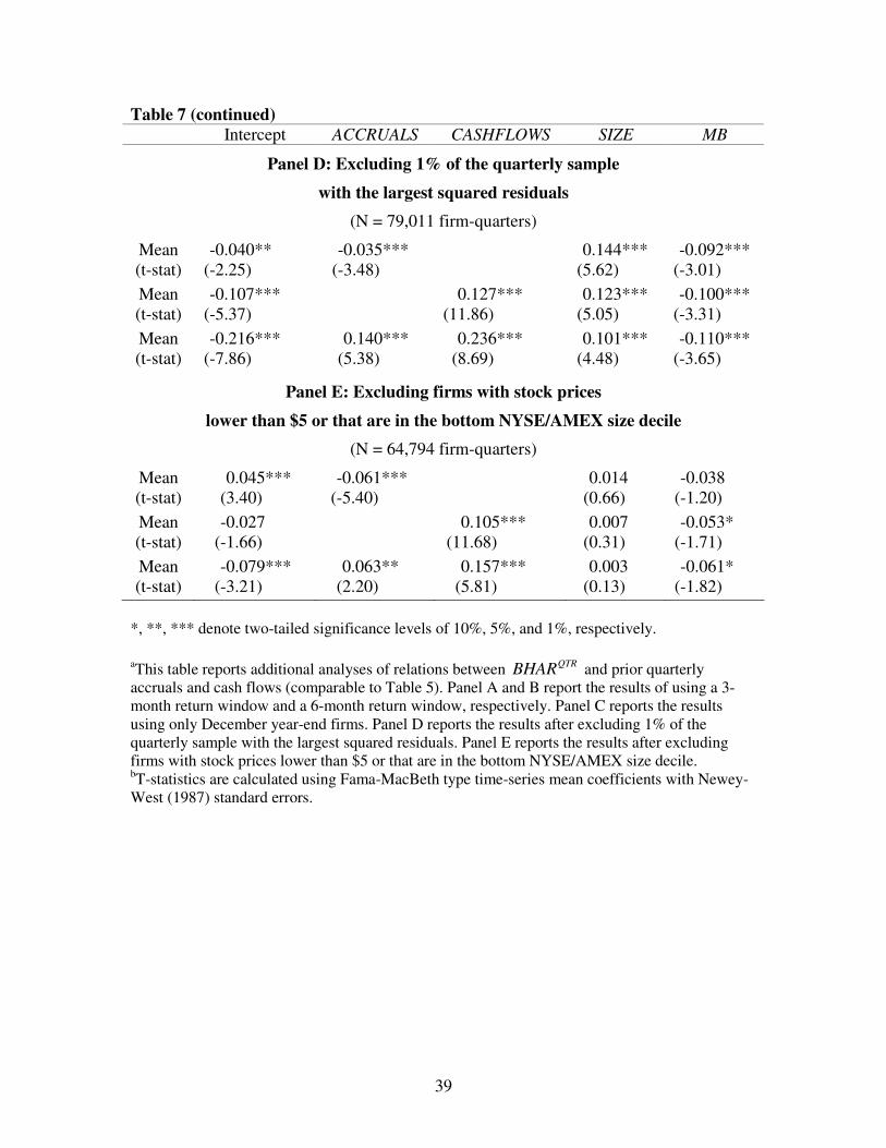
39

Table 7 (continued) Intercept ACCRUALS CASHFLOWS SIZE MB

Panel D: Excluding 1% of the quarterly sample

with the largest squared residuals

(N = 79,011 firm-quarters)

Mean (t-stat)

-0.040** (-2.25)

-0.035*** (-3.48)

0.144*** (5.62)

-0.092*** (-3.01)

Mean (t-stat)

-0.107*** (-5.37)

0.127*** (11.86)

0.123*** (5.05)

-0.100*** (-3.31)

Mean (t-stat)

-0.216*** (-7.86)

0.140*** (5.38)

0.236*** (8.69)

0.101*** (4.48)

-0.110*** (-3.65)

Panel E: Excluding firms with stock prices

lower than $5 or that are in the bottom NYSE/AMEX size decile

(N = 64,794 firm-quarters)

Mean (t-stat)

0.045*** (3.40)

-0.061*** (-5.40)

0.014 (0.66)

-0.038 (-1.20)

Mean (t-stat)

-0.027 (-1.66)

0.105*** (11.68)

0.007 (0.31)

-0.053* (-1.71)

Mean (t-stat)

-0.079*** (-3.21)

0.063** (2.20)

0.157*** (5.81)

0.003 (0.13)

-0.061* (-1.82)

*, **, *** denote two-tailed significance levels of 10%, 5%, and 1%, respectively. aThis table reports additional analyses of relations between QTRBHAR and prior quarterly accruals and cash flows (comparable to Table 5). Panel A and B report the results of using a 3-month return window and a 6-month return window, respectively. Panel C reports the results using only December year-end firms. Panel D reports the results after excluding 1% of the quarterly sample with the largest squared residuals. Panel E reports the results after excluding firms with stock prices lower than $5 or that are in the bottom NYSE/AMEX size decile. bT-statistics are calculated using Fama-MacBeth type time-series mean coefficients with Newey-West (1987) standard errors.

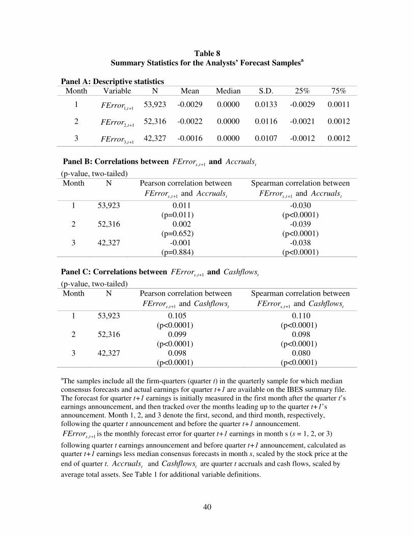
40

Table 8 Summary Statistics for the Analysts’ Forecast Samplesa

Panel A: Descriptive statistics

Month Variable N Mean Median S.D. 25% 75%

1 1,1 +tFError 53,923 -0.0029 0.0000 0.0133 -0.0029 0.0011

2 1,2 +tFError 52,316 -0.0022 0.0000 0.0116 -0.0021 0.0012

3 1,3 +tFError 42,327 -0.0016 0.0000 0.0107 -0.0012 0.0012

Panel B: Correlations between 1, +tsFError and tAccruals (p-value, two-tailed) Month N

Pearson correlation between

1, +tsFError and tAccruals Spearman correlation between

1, +tsFError and tAccruals 1 53,923 0.011

(p=0.011) -0.030

(p<0.0001) 2 52,316 0.002

(p=0.652) -0.039

(p<0.0001) 3 42,327 -0.001

(p=0.884) -0.038

(p<0.0001) Panel C: Correlations between 1, +tsFError and tCashflows (p-value, two-tailed) Month N Pearson correlation between

1, +tsFError and tCashflows Spearman correlation between

1, +tsFError and tCashflows

1 53,923 0.105 (p<0.0001)

0.110 (p<0.0001)

2 52,316 0.099 (p<0.0001)

0.098 (p<0.0001)

3 42,327 0.098 (p<0.0001)

0.080 (p<0.0001)

aThe samples include all the firm-quarters (quarter t) in the quarterly sample for which median consensus forecasts and actual earnings for quarter t+1 are available on the IBES summary file. The forecast for quarter t+1 earnings is initially measured in the first month after the quarter t’s earnings announcement, and then tracked over the months leading up to the quarter t+1’s announcement. Month 1, 2, and 3 denote the first, second, and third month, respectively, following the quarter t announcement and before the quarter t+1 announcement.

1, +tsFError is the monthly forecast error for quarter t+1 earnings in month s (s = 1, 2, or 3)

following quarter t earnings announcement and before quarter t+1 announcement, calculated as quarter t+1 earnings less median consensus forecasts in month s, scaled by the stock price at the end of quarter t. tAccruals and tCashflows are quarter t accruals and cash flows, scaled by average total assets. See Table 1 for additional variable definitions.

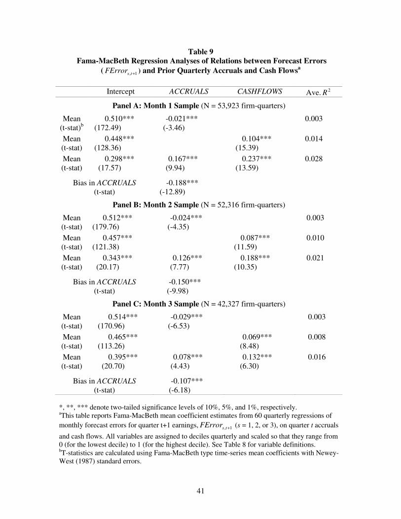
41

Table 9 Fama-MacBeth Regression Analyses of Relations between Forecast Errors

( 1, +tsFError ) and Prior Quarterly Accruals and Cash Flowsa

Intercept ACCRUALS CASHFLOWS Ave. 2R

Panel A: Month 1 Sample (N = 53,923 firm-quarters)

Mean (t-stat)b

0.510*** (172.49)

-0.021*** (-3.46)

0.003

Mean (t-stat)

0.448*** (128.36)

0.104*** (15.39)

0.014

Mean (t-stat)

0.298*** (17.57)

0.167*** (9.94)

0.237*** (13.59)

0.028

Bias in ACCRUALS (t-stat)

-0.188*** (-12.89)

Panel B: Month 2 Sample (N = 52,316 firm-quarters)

Mean (t-stat)

0.512*** (179.76)

-0.024*** (-4.35)

0.003

Mean (t-stat)

0.457*** (121.38)

0.087*** (11.59)

0.010

Mean (t-stat)

0.343*** (20.17)

0.126*** (7.77)

0.188*** (10.35)

0.021

Bias in ACCRUALS (t-stat)

-0.150*** (-9.98)

Panel C: Month 3 Sample (N = 42,327 firm-quarters)

Mean (t-stat)

0.514*** (170.96)

-0.029*** (-6.53)

0.003

Mean (t-stat)

0.465*** (113.26)

0.069*** (8.48)

0.008

Mean (t-stat)

0.395*** (20.70)

0.078*** (4.43)

0.132*** (6.30)

0.016

Bias in ACCRUALS (t-stat)

-0.107*** (-6.18)

*, **, *** denote two-tailed significance levels of 10%, 5%, and 1%, respectively. aThis table reports Fama-MacBeth mean coefficient estimates from 60 quarterly regressions of monthly forecast errors for quarter t+1 earnings, 1, +tsFError (s = 1, 2, or 3), on quarter t accruals

and cash flows. All variables are assigned to deciles quarterly and scaled so that they range from 0 (for the lowest decile) to 1 (for the highest decile). See Table 8 for variable definitions. bT-statistics are calculated using Fama-MacBeth type time-series mean coefficients with Newey-West (1987) standard errors.