Do informal transfers induce lower efforts?

Evidence from lab-in-the-field experiments in rural Mexico∗

Ingela Alger†,

Laura Juarez‡,

Miriam Juarez-Torres§,

Josepa Miquel-Florensa¶

September 4, 2018

Abstract

How do informal transfers affect work incentives? The question matters in developing countries, where

labor markets are intertwined with transfer networks. The tax-and-subsidy component of transfers would

dilute work incentives, but their pro-social element could encourage people to work harder. Such crosscur-

rents are hard to disentangle because participation in informal networks is likely endogenous. We tackle this

problem with a lab-in-the-field experiment that uses a real-effort task. Our main finding is that participants

do not reduce their effort in the presence of transfers. This suggests that the impact of informal transfers

may extend beyond just the sharing of risk.

Keywords: informal transfers, effort, moral hazard, warm glow, altruism

JEL codes: D64, C91, O12

∗We thank the Agence Nationale de la Recherche for funding this research through a grant awarded to Ingela Alger (Chaire

d’Excellence ANR-12-CHEX-0012-01). Support by ANR-Labex IAST is also gratefully acknowledged. Ingela Alger and Josepa

Miquel-Florensa further gratefully acknowledge the generous hosting by Banco de Mexico. Part of this research was conducted

while Laura Juarez was a researcher at Banco de Mexico. We are indebted to Ing. Mario Rivera de Labra (INIFAP Campeche),

whose help was invaluable. We thank Matteo Bobba, Donald Cox, Salvatore Di Falco, Marcel Fafchamps, Rocco Macchiavello,

Cesar Mantilla, Mohamed Saleh, and participants at the Asian Meetings of the Econometric Society 2016 in Kyoto, the Barcelona

Summer Forum, SEEDC 2016 Workshop, LACEA 2016, 2017 ASSA Meetings and seminar participants at GATE Lyon, University

of Geneva, Universidad Javeriana, and the World Bank for useful comments and suggestions. Finally, this paper would not have

seen the light of day without the outstanding research assistance, both in the field and in the office, provided by Mariana Garcia

and Ildrim Valley. The views expressed in this article are solely those of the authors and do not necessarily reflect those of Banco

de Mexico.

†Toulouse School of Economics, CNRS, University of Toulouse Capitole, Toulouse, France, and Institute for Advanced Study in

Toulouse. ingela.alger@tse-fr.eu

‡El Colegio de Mexico. laura.juarez@colmex.mx

§Banco de Mexico. mjuarez@banxico.org.mx

¶Toulouse School of Economics, University of Toulouse Capitole, Toulouse, France. pepita.miquel@tse-fr.eu

1

1 Introduction

Informal transfers are widespread in most developing countries.1 While such transfers allow the sharing of risk

for any given income distribution,2 they may also affect the income distribution itself by distorting the incentives

to undertake productive efforts or save in the first instance. Any relationship between transfers and efforts may

be quite important in economies in which informal transfers are common: if transfers have a detrimental effect

on effort, they may hamper economic development; if they have a positive effect on effort, they help promote

economic development above and beyond the benefits of risk sharing. To evaluate the overall effects of informal

transfers on welfare, it is therefore crucial to understand whether or not, and how, they affect the incentives to

undertake productive efforts.

Several recent empirical studies conducted in Africa suggest that “kin taxes” have a detrimental incentive

effect. Thus, Azam and Gubert (2005) and Baland et al. (2016) find that being on the receiving end of transfers

(from emigrated relatives in the former study, from older siblings in the latter study) induces reduced work

efforts. Di Falco and Bulte (2013) show that the presence of relatives induce lower levels of self-protection. The

empirical analyses of Alby, Auriol, and Nguimkeu (2013), Grimm, Hartwig, and Lay (2016), and Squires (2016)

indicate that kin taxes may be a significant barrier to entrepreneurship. Finally, a number of empirical and

experimental studies, including Baland, Guirkinger, and Mali (2011), Di Falco and Bulte (2011), Jakiela and

Ozier (2016), and Boltz, Marazyan, and Villar (2016), suggest that some people appear to undertake strategies

to avoid having to share with kin.3

Such disincentive effects are exactly what would be expected if individuals are selfish and transfers are driven

by a desire to comply with a social norm. However, if transfers are instead driven by an intrinsic desire to

share (e.g., altruism or warm glow), they may in theory have a positive effect on productive efforts (Alger and

Weibull, 2008, 2010). In this paper we report the results of a novel experiment designed specifically to provide

insights on how the anticipation of making or receiving a transfer affects the incentives to undertake productive

efforts. Compared to the literature, our experimental design introduces two novel features: it imposes the size

and direction of transfers, and it relies on a real effort task. These features present two advantages. First,

since subjects do not choose the transfers, the design allows to separate effort choice from transfer choice,

a separation which cannot be obtained with empirical data, for which both effort and transfer decisions are

endogenous. Second, since subjects choose a real effort instead of an investment from an endowment, the design

makes it possible to obtain a measure of the motivation to exert effort in the presence of transfers, which is

not tainted by the marginal utility of money. Our experiment is also novel in that it studies the effects of

both giving and receiving transfers, whereas the literature has focused on the effects of giving transfers only.

We further contribute to the literature on forced solidarity and incentives by conducting the experiment on a

population outside Africa. By contrast to the findings cited above, we find that on average the anticipation of

making and of receiving a transfer does not have a negative impact on effort.

In reality, informal transfers are often embedded in long-term, repeated interactions, in which the willingness

to provide effort may be driven by a strategic repeated-interaction effect (Ligon, Thomas, and Worrall, 2002),4

1For a cross-country analysis, see Cox, Galasso and Jimenez (2006). See also Cox and Fafchamps (2008) for a survey of the

literature on extended kinship networks, and Fafchamps (2011) for a survey of the literature on inter-household transfers.

2For evidence on such sharing of risk, see Rosenzweig (1988), Udry (1990), Townsend (1994), Ligon, Thomas and Worall (2002),

Fafchamps and Lund (2003), Dercon and Krishnan (2003), Dubois, Jullien, and Magnac (2008), Mobarak and Rosenzweig (2013),

and Attanasio, Meghir, and Mommaerts (2015).

3The field experiment conducted by Di Falco, Feri, Pin, and Vollenweider (2017) on how farmers allocate relatives’ labor inputs

in response to the productivity of their maize variety is also relevant in this context.

4See also Kimball (1988), Coate and Ravallion (1993), and Kocherlakota (1996).

2

or by a desire to signal pro-sociality (Benabou and Tirole, 2006). Furthermore, participation in such interactions

is often voluntary. Hence, in reality an individual’s effort choice is likely affected by a complex set of factors,

which, moreover, may interact. In order to understand the overall effects of these factors and how they may

interact, a necessary first step is to study each of them in isolation. Thus, the decision to participate in risk-

sharing groups has been studied by Barr and Genicot (2008) and Attanasio et al. (2012). We study another

question, namely, does the potential pro-social element of transfers, which would encourage people to work

harder, outweigh the tax-and-subsidy component of transfers, which dilutes work incentives?

To study this question, we propose an experimental design that imposes the composition of the group

within which transfers take place, and that shuts down both the repeated-interaction and the signaling channel.

Thus, we disregard limited commitment, by examining behavior in one-shot interactions, and we impose the

direction as well as the size of any transfer, so that the only choice variable for subjects is the productive

effort. Specifically, in this experiment each subject played four games. In each game the subject received

an endowment and was given an opportunity to perform a real effort. The effort level chosen by the subject

determined the probability of success, where success meant that additional income was generated on top of

the initial endowment. In autarky games, the subject was simply able to keep any such additional income. In

transfer games, subjects allocated to a donor role had to make a transfer (of fixed size) to someone else in case

of success. Subjects allocated to a recipient role received a transfer (of fixed size) from someone else in case of

failure. In any case, individuals who were potentially affected by these transfers were passive, so there was no

strategic interaction. Reciprocity and signaling motives were ruled out, as much as possible, by ensuring that

effort choices as well as payoffs were private information, and by matching subjects anonymously.

In the absence of other confounders, the comparison of effort choices in autarky games with those in transfer

games provides a clean measure of how the mere anticipation of making or receiving a transfer affects effort.

However, the choice of a real effort task for our experiment arises two potential concerns: ability and learning

in performing the task. We control for the baseline ability with individual fixed effects in all of our estimations.

Controlling for learning is particularly relevant in our design because the autarky games were always played

before the transfer games in each treatment to avoid priming. We account for learning with two alternative

approaches: first, by using observed effort as a dependent variable and including round dummies in our main

estimations; and second, by estimating a linear learning model using the first two autarky games in one of our

treatments, predicting effort in subsequent rounds for all observations, and then using the difference between

predicted and observed effort as a dependent variable.

Importantly, in the autarky and transfer games played by any given subject, effort had the same effect on

the expected amount paid by us to the community. Hence, if subjects made a greater effort in the presence of a

transfer, this cannot be explained by a desire to extract more money from the experimenters. Instead, an effort

increase can only be explained by a positive utility associated with giving a transfer when in a donor role and

with avoiding receiving a transfer when in a recipient role.

In economics many classes of pro-social preferences have been studied, including altruism (Becker, 1974),

warm glow (Andreoni, 1990), a concern for fairness or inequity aversion (Rabin, 1993; Fehr and Schmidt,

1999), caring about social efficiency (Charness and Rabin, 2003), and moral concerns (Alger and Weibull,

2013). It is beyond the scope of this paper to make a full analysis of all these preference classes. Instead, we

limit our attention to the following three: selfishness, altruism, and warm glow. The payoff structures in the

experiment allow us to infer whether the observed behaviors are more consistent with selfishness, altruism, or

warm glow preferences. The focus on altruism and warm glow is natural in the context of transfers, because

these preferences would result in different responses in the event that public transfers were introduced: indeed,

public transfers would crowd out individual pro-social behaviors less if these are driven by warm glow than if

3

they are driven by altruism.

The experiment was conducted in 16 small villages in rural Mexico (where informal transfers are common),5

with a total of 536 participants. Within each village, the participants were randomly split into two groups,

one of which was allocated to a donor treatment with transfers going to passive recipients, and the other to a

recipient treatment with transfers coming from passive donors. Across villages, we varied the transfer size: in

half of the villages the transfer represented 33% of the additional income, while in the other half the transfer

represented 100%. While the former is more realistic, the latter allows to draw strong conclusions. Indeed, even

in the presence of potential learning confounders, if subjects make some effort at all when the transfer is 100%

of the additional income, it must be that they derive utility from the transfer.

Our main findings are as follows. First, we find that transfers do not decrease effort. Most of our preferred

estimates of the effect of transfers, i.e., those based on the learning model correction, are positive, although only

a few are marginally significant. Second, since this is true even in treatments where the transfer represents 100%

of the potential additional income, and since the expected amount of money extracted from the experimenter

is held constant across the games played by any subject, we can safely conclude that, on average, subjects

derive positive utility from transfers.6 In particular, the hypothesis that selfishness (or worse, spite) is the main

motivation in the sample can be ruled out. Moreover, while in most cases we cannot conclude whether the

behaviors lend more support to warm glow or to altruistic preferences, our finding that recipients do not change

their effort significantly in response to a transfer, compared to autarky, is more in line with warm glow than

with altruism, for no level of altruism could explain this response, as shown in the theoretical analysis.

We also provide suggestive evidence on whether the effort exerted in the transfer games varies with the

identity of the passive party affected by the transfer. Specifically, we find positive, larger and slightly more

significant effects when the transfer affects another individual drawn at random from a group of passive partic-

ipants, than when it affects the whole pool of passive participants. However, the hypothesis that both effects

are equal cannot be rejected. Additional results on heterogeneous effects suggest that the effect of transfers on

effort increases, and thus it is more likely to be positive, with the religious homogeneity of the village.7

Our results are consistent with observations of pro-social behaviors in laboratory experiments.8 In particular,

they are qualitatively in line with findings in anonymous dictator games, where positive transfers suggest that

the subjects derive a benefit from giving in such situations (Blanco, Engelmann, and Normann, 2011).9 Such

5There is a large literature on behaviors in small villages in Mexico (e.g., Angelucci, De Giorgi, Rangel, and Rasul, 2009, 2010).

6This finding further allows us to rule out the possibility that subjects seek to earn a target income (Camerer et al., 1997):

indeed, if this motivation was driving their behavior, they should make no effort in treatments where the transfer represents 100%

of the potential additional income. Moreover, note that since effort generates the same expected additional income for the subject

pool as a whole across the games, a higher effort in the presence of transfers would be inconsistent with full ex post sharing within

the subject pool.

7Even though our subjects do not know the individual identity of the donor or recipient with whom they are being paired,

in villages that are more homogeneous in terms of religious denomination the likelihood of being paired with another individual

who shares the subjects’ religious beliefs is higher, and this can have an effect on sharing behavior. Relatedly, Barr, Dekker and

Fafchamps (2012) find that individuals belonging to the same religious group are more likely to share risk when agreements are

enforced through social sanctioning than when they are so by the experimenter. Regarding other economic outcomes, Fisman,

Paravisini and Vig (2012) show that shared religious beliefs between borrowers and lenders affect outcomes like loan amounts and

repayment. Finally, these results are in line with Leider et al. (2009), who find that helping behaviors tend to be different towards

friends than towards strangers, and the idea that an individual’s behavior may depend on her sense of identity, which may depend

on political, religious, educational, cultural, gender, or other identifying factors (Akerlof and Kranton, 2000; see also Kranton,

2016, and Kranton et al. 2016).

8For a recent survey see DellaVigna (2009).

9If given the possibility to pay a price to avoid giving, however, some subjects use this option (see, e.g., Dana, Weber, and

4

findings have also been made in experiments in developing countries, with variations on the anonymity of the

recipient and the origin of the income to be shared.10 Furthermore, the fact that our results lend stronger support

to warm glow than to altruism is in line with other (different) experiments that have sought to discriminate

between these two motives, including Palfrey and Prisbrey (1996), Erkal, Gangadharan, and Nikiforakis (2011),

and Gangadharan et al. (2016).11

If externally valid, our findings suggest that informal transfers in our participating villages may allow risk

to be shared without having a negative impact on productive efforts. However, as is well known external

validity is by no means a trivial matter (Levitt and List, 2007). Three caveats may be particularly relevant

here. First, in our experiment subjects undertake effort for a short amount of time, while in reality productive

efforts take place over extended periods of time. Second, in reality individuals may use productive efforts and

transfers as substitutes in order to assist others: hence, even if in reality it was possible to disentangle effort

and transfer choices, it is not clear that transfers would be positively correlated with productive efforts. Third,

the population we sample is exposed to the communal land system known as ejido. It is possible that this has

a positive impact on pro-sociality.12

The experiment is described in the next section, with the theoretical model presented and analyzed in

Section 3. The empirical specification is described in Section 4, the results are presented in Section 5, followed

by robustness checks in Section 6. Section 7 concludes.

2 The effort-and-transfer experiment

2.1 Experimental design and session structures

Each subject played a series of four games, one of which was randomly drawn at the end of the experimental

session to determine the payoffs; hence, the games were seen as independent by the participants. Each subject

also received a payoff from being a passive party for other subjects, but since (s)he had no influence on this

payoff, (s)he was informed about it only at the moment (s)he was paid. In each game the subject was presented

with the same initial endowment and the same real effort task. The subject’s effort level determined the

probability that additional income was generated. All subjects played both autarky and transfer games: in

autarky games, nothing else happened besides the effort and the ensuing potential generation of additional

income; in transfer games, a transfer sometimes occurred between the subject and another, passive, party.

Importantly, in all the transfer games the transfer direction and size were exogenously imposed. Hence, the

Kuang, 2007, DellaVigna, List, and Malmendier, 2012, and Lazear, Malmendier, and Weber, 2012). Our experiment did not include

such an option.

10Thus, Ligon and Schechter (2012) conclude that the largest proportion of observed transfers in anonymous dictator games

among villagers in rural Paraguay can be attributed to preference-related motives. Jakiela (2015) compares the behavior of U.S.

students to Kenyans to study whether the willingness to share is different when the endowment in the dictator game derives from

luck and when it is the result of a risk-free effort. In a comparative experimental study in which subjects could give own wealth,

or steal or destroy others’ wealth, Fafchamps and Vargas-Hill (2015) found that some gave and some stole, and that Kenyan and

Ugandan subjects behaved more pro-socially than British subjects.

11There is also a non-experimental empirical literature that seeks to tease out the motivations behind transfers. See, e.g., Lucas

and Stark (1985), Altonji, Hayashi, and Kotlikoff (1992), Cox, Eser, and Jimenez (1998), Foster and Rosenzweig (2001), De la

Briere et al. (2002), and De Weerdt and Fafchamps (2011). However, the results reported in this literature are not directly

comparable to ours, since empirical work relying on real-life transfers cannot shut down the reciprocity motive.

12To wit, Carpenter and Seki (2011) find that fishermen exposed to teamwork act more prosocially in public goods games than

those who are not exposed to teamwork.

5

subject’s only decision consisted in the level of effort to exert. Across the subjects we varied the role (donor vs

recipient), as well as the transfer size, which was either partial (33% of the additional income) or full (100% of

the additional income). While a partial transfer may be closer to real-life settings, the full transfer allows us to

single out how a transfer affects effort when the effort has no effect on own wealth. This two-by-two design thus

resulted in four treatments: Donor-Partial (DP), Recipient-Partial (RP), Donor-Full (DF), and Recipient-Full

(RF). In the two Donor treatments, a subject who had successfully generated additional income had to make

a transfer to a passive party. In the two Recipient treatments, a subject who had failed to generate additional

income received a transfer from a passive party.

The experiment was conducted in 16 villages, each of which was allocated randomly either to the Partial

or to the Full treatments. In each village the subject pool was divided randomly into two groups of equal size

(usually 20), one of which was allocated to the Donor treatment, and the other to the Recipient treatment.

The Donor and the Recipient treatments were run one after the other. Whichever group of individuals was not

actively playing, was used (unbeknownst to these individuals) as passive players in some of the games played by

the individuals in the active group. In sum, then, any subject in a Donor treatment was an active transfer donor

and a passive transfer recipient, while any subject in a Recipient treatment was an active transfer recipient and

a passive transfer donor.

The first four of the six boxes in Figure 1 show the games played in the four treatments (the Partial

treatments are in the left column and the Full treatments in the right column), and the payoff consequences of

success (S) and failure (F) in each game, both to the active subject and to the associated passive party (the first

number is the initial endowment, an italicized number the additional income, and a bold number a transfer).13

The following set of three games was qualitatively similar across the four treatments: the Autarky game, the

One-to-One game, and the Pool game. In the One-to-One game each active subject was matched anonymously

with one passive individual (and each passive individual was matched only with this active subject); in the Pool

game the passive party was the pool of passive individuals, who were all equally affected by any transfer to/from

an active subject (in Figure 1, n denotes the total number of passive subjects, ns the number of other active

subjects who succeeded, and nf the number of other active players who failed). Note that in each treatment

the subject’s initial endowment as well as the additional income was the same in these three “core” games;

furthermore, the transfer amount as well as the initial endowment to any passive player was the same in both

of these transfer games, and the active subject was always at least as rich as any passive transfer recipient.

On top of the three core games, which are used for the main analysis, two additional variations were

introduced. First, subjects in the Partial treatments played an Autarky Low game. This game had the same

net effect on the active player’s payoff as the transfer games, and thus allows to compare two payoff-equivalent

games, one with and one without a transfer. Second, subjects in the Full treatments played a Public transfer

game, where the transfer source/destination was the health center of the village, i.e., outside of the experimental

setting. The Public game will be used for a robustness test, because it differs from the core transfer games

in that the transfer no longer affects the participants in the experiment directly, but the village to which they

belong. Thus, the Public game can be used to determine to what extent in the core games subjects are driven

by a desire to extract money from us to the subjects.

Upon completing the games and the ability tests (see more on these below), and while the subjects were still

in the lab, all subjects were asked post-experimental questions. First, subjects were asked questions pertaining

13All the numbers are expressed in points, the experimental unit, worth MXN 0.50 each (when the experiment was conducted,

the exchange rate was approximately MXN 13 = USD 1). The overall average payoff turned out to be MXN 92 (it was MXN

59.55.across the Donor-Full treatments, MXN 122.02 across the Donor-Partial treatments, MXN 62.30 across the Recipient-Full

treatments, and MXN 122.43 across the Recipient-Partial treatments).

6

to the One-to-one game. In the Donor-Partial treatment we asked subjects if they would have liked to give

more than 25, in the Donor-Full treatment we asked if they would have liked to give less than 75, and how much

more/less in case of a positive answer. This allows us to check whether the results are driven by the transfer size

being imposed by us. Second, we asked each subject in the Recipient treatments if (s)he would reveal his/her

effort level to the individual with whom (s)he was matched in the One-to-one game if given the opportunity

to do so. The answers to this question will allow to check if the results were driven by the non-observability of

effort.

At the very end of the session, subjects filled out a questionnaire with questions pertaining to standard

individual characteristics and transfer behaviours in the past year.

The two boxes at the bottom of Figure 1 summarize the session structures. There were two alternative

orders for the Partial treatments and two alternative orders for the Full treatments.

2.2 The nuts-and-bolts effort task

Given our focus on effort choices, we propose a real effort instead of a “chosen effort” (Bruggen and Strobel,

2007) task. We do so for two reasons: because it removes income effects, and because the population that

was sampled for the experiment might be unaccustomed to abstract reasoning. The effort task consisted of

threading nuts onto bolts.14 For each fully threaded nut (all the nut-bolt pairs were identical), the subject

increased the probability of generating additional income by 0.1, a probability which was zero for zero threaded

nuts.15 Ten fully threaded nuts thus guaranteed success. In each game the subject had one minute to thread

nuts onto bolts.16 Curtains ensured that subjects could not observe each other’s effort choices or communicate.

Furthermore, to minimize the experimental pressure to exert effort, each subject had on his/her table a fresh

newspaper to look at during the imparted time.

Clearly, threading nuts onto bolts in a short period of time is a task that requires ability. To get measures

of ability, we let each subject take two incentivized ability tests, one at the beginning and one at the end of the

experimental session. Each ability test consisted in rewarding the participants with one point for each properly

threaded nut in one minute. The first ability test gives us information on baseline ability in performing the

task. In Appendix B.2, we show that the baseline ability distribution, as measured with this first test, does not

differ significantly across treatments and roles. Furthermore, in our main specifications, we include individual

fixed effects to control for baseline ability and for any other individual-specific factors that might affect effort

14A variety of real effort tasks have been used in the literature, such as solving anagrams (Charness and Villeval, 2009), stuffing

envelopes (Carpenter et al., 2010), counting zeros (Abeler et al., 2011), and moving sliders (Gill and Prowse, 2012). We chose a

manual task that did not require the use of computers, and which allowed us to use the same materials in all the sessions without

experiencing damage.

15Concretely, for each fully threaded nut, the subject earned one ball. Thus, upon completing the four games, each subject had

earned a certain number (between 0 and 10) of balls in each game. Once the game that would be used to calculate the payoffs

had been picked, a traditional style bingo cage with balls numbered from one to ten was used to draw one ball. Any subject who

had threaded a number of nuts equal to or greater than the number on the ball drawn in the relevant game generated additional

income, whereas those who had threaded a smaller number did not generate additional income.

16In the theory section below, we assume that the cost of effort is strictly convex in effort. This allows us to focus on interior

solutions. In the experiment the probability of success is linearly increasing in the number of threaded nuts and it may therefore

appear that the cost of effort is linear. However, since subjects were time-constrained effort really consisted in the speed at which

nuts were threaded, it is sensible to believe that marginal cost of effort was indeed increasing in effort. Furthermore, the fact that

out of 2,144 observations (536 participants who played four games each) there are 23 observations where zero nuts were threaded,

and 209 where ten nuts were threaded, indicates that our focus on interior solutions is sensible. It may also be that the subjects

enjoyed performing the task. This concern is irrelevant for our main results, which rely on within-subject comparisons of efforts.

7

and that remained constant throughout the session.

Given that the effort task is performed repeatedly, learning may also arise in our experiment. This is of

particular concern in our case because we always let the subjects play the transfer games after the autarky

game(s) to avoid the priming that the introduction of a transfer, and its subsequent removal, could induce

and because of the pedagogical advantage of starting with the simplest game in a population unaccustomed to

abstract reasoning (see Figure 1). Thus, subjects might have accumulated more learning when they play the

transfer games than when they play the autarky game(s). Since our empirical strategy consists in comparing

the effort in the transfer games to the effort in the autarky game(s), learning is a potential confounding variable

that must be adequately controlled for.

We adopt two alternative approaches to control for learning in our estimations that compare effort between

the transfer and autarky games. First, we include round dummies in the regressions. As mentioned, the autarky

games were always played before the transfer games, and the order between the transfer games (One-to-One

versus Pool) was varied. As a result, this approach accounts for the fact that the games being compared are

played in different rounds for different session orders, letting the dummies absorb the difference arising from

additional rounds of practice. Second, as detailed next, we estimate a simple learning model and then use the

results of this model to purge observed effort from potential learning.

To get an estimate of learning, we use the effort observed in the two autarky rounds played in the Partial

treatments.17 These two games are comparable: they both involve risk, the same initial endowment, and no

transfers. Their similarity is crucial to attribute most of the difference in effort between these two rounds in

the Partial treatments to learning, i.e., to the effect of an additional round of practice on the number of nuts

threaded.18 The only difference between them is that the expected return to effort is lower in the Autarky Low

game, compared to the Autarky game. However, since the mean difference in effort between these two games is

not statistically significant (see Appendix B.3), it is arguably sensible to pool them in our learning estimation.19

Given that the two autarky games in the Partial treatments were played right after the first ability test,

our learning estimate would reflect the learning about the effort task that occurs relatively early in the session.

Furthermore, by using these two autarky games, which were played before the introduction of any transfers, we

ensure that our estimated learning does not incorporate any of their effect on effort.

Let eir denote effort of individual i in the autarky game played in round r in a partial treatment, where

r = 1, 2. We estimate the average change in effort between those two rounds, which we attribute mostly to

learning, with the following regression:

ei2 = η ∗ ei1. (1)

We then use the estimated value η to calculate, for each individual i, the predicted effort in each round r = 2, 3, 4

of the experiment as follows:

eir = η(r−1) ∗ ei1, (2)

17We thank the Associate Editor, who remained anonymous, for suggesting this method.

18We refrain from using the first ability test for estimating learning because the points per threaded nut in the practice rounds

and the autarky rounds were different; the payoff was deterministic in the ability test rounds but stochastic in the autarky rounds;

the subjects were sure that they would get the payoff earned in the practice rounds but there was only a 25% chance that any

given autarky round would be used as basis for payment; and effort was not bounded above in the practice rounds as it was in the

autarky and transfer rounds.

19As complementary evidence, we also perform a difference-in-differences (DD) estimation using the fact that, by design, the

first two experimental games in the Partial treatment are autarkies, whereas the first and second games in the Full treatment

are an autarky game and a transfer game, respectively. The details and results of this alternative, suggested anonymously by the

Associate Editor, are in Appendix B.4.

8

where ei1 is i’s effort in the first of the four games after the initial ability test, which is always an autarky

game. This approach assumes that subjects learn at a constant rate in each subsequent round, equal to the

estimated rate between the first two games. We use the effort in the first game (r = 1) to calculate the effort

in all subsequent rounds, instead of the effort in the corresponding previous round, to avoid any contamination

of the predicted effort due to presence of transfers in the later rounds.

As a final step in this approach, we estimate our main specifications (see Section 4) using observed effort

for round r = 1 and the following measure of “clean” effort, i.e., effort purged from learning effects, for rounds

r = 2, 3, 4:

ecir = eir − eir. (3)

The results of the learning estimation and a comparison between raw and “predicted” efforts are presented

in detail in Appendix B.3. In that appendix, for robustness we also present the results of a learning estimation

using a linear specification with a constant, and a and a log-linear specification with a constant. In general, the

results of these robustness checks are consistent with those obtained with the learning specification described

in this section.

2.3 Procedures

In each of the 16 villages where a session took place, subjects were recruited by way of public announcements

supported by the village authorities, a day before as well as on the day of the session.20 Applying a “first come,

first served” rule for men and women separately, in each village we sought to obtain a total of 40 subjects,

gender-balanced whenever possible. At most one representative per household could participate; furthermore,

although we selected small localities (see Table C1), the questionnaire data suggest that only a small share

of the subjects were first-degree relatives (see Table 1). Upon arrival, each participant picked a card from an

opaque bag. Each card had a number that allowed us to track the subject anonymously, and a symbol that was

used to assign the participant to one of the two groups. Half of the subjects were thus led to the lab field, while

the other half were shown to another room; the latter group got a snack while waiting for their turn to be led

to the field lab. In the One-to-one games, the active subjects were randomly and anonymously matched with

the passive subjects, so that each active and each passive subject was matched with exactly one individual. In

the Pool games any transfer affected all the passive individuals equally.

Almost all the sessions were conducted in the afternoon, after the end of the agricultural labour day, in the

village’s own school building.21 These buildings all had at least two independent rooms, one of which was used

as the field lab and another one as a waiting room for the passive subjects. The lab rooms were large enough

to contain twenty tables and chairs arranged in four columns; all subjects faced the experiment director and

could properly see her and hear the instructions. We installed opaque curtains between the columns to provide

privacy for the subjects (they could not see above the backs of those sitting in front of them, and they were

not allowed to turn around to look at those sitting behind them). The experiment director was the same in

all the sessions. No written instructions were provided, the protocol was read out loud (and clarified in case of

need) and all materials were visual and text-free due to the low literacy levels of the participants. Protocols

and experimental materials can be found in the Appendix. Translation of the instructions by a native Mayan

speaker was provided in those villages where some subjects did not understand Spanish.

20Public announcements consisted of loudspeaker announcements and written ads, and by the village authorities spreading the

information within the village.

21All took place in a primary school, except two, that took place in a high school and in an ejido meeting hall, respectively.

9

In the lab room, each subject sat in front of the table assigned to his or her number. On the table there was

one bowl with nuts and one with bolts, as well as a fresh newspaper. Participants were explicitly instructed

to not touch any material before receiving the instruction to do so from the experiment director. When the

first group had completed the ability tests and the games, and had answered the question(s) (see Figure 1), the

two groups would quietly change rooms without interacting. The first group then got a snack and completed

the post-experimental questionnaire in the auxiliary room; the second group filled out this questionnaire, also

in the auxiliary room, upon having completed its session in the field lab room. Illiterate participants received

help by a native Mexican assistant or Mayan native speaker to fill out the questionnaire.

Once both groups had performed their experimental session, a child randomly picked a colored card (from

an opaque bag) in front of everybody; the card determined which of the four games would be used to calculate

the payoffs (if it was the one-to-one game, then it was the one-to-one game both for donors and for recipients,

etc). Finally, to ensure transparency of the payments calculation, the lottery was performed in front of all the

participants. The average payment was 92 pesos, close to the minimum wage of an agricultural worker.22

Each group spent between 30 and 45 minutes in the field lab room, depending on the need for translation.

The complete session, from the arrival to the the departure of the subjects, usually lasted about three hours.

2.4 Field setting and locality selection

The experimental sessions were conducted in July 2014 in the state of Campeche, Mexico. Although the

predominant economic activity in Campeche is oil and natural gas extraction (84% of the state GDP according

to the National Economic Census 2014), its inhabitants are poor: 43.6% of the state’s population is in poverty

situation and 11% in extreme poverty (source: CONEVAL 2015).23 Agricultural activities represent 0.5% of

the state GDP in 2014 (source: National Economic Census 2014). Campeche’s soils are poorly suited for

agriculture, and an important proportion of the agriculture is developed by small and self-subsistence farmers;

water is more abundant in the South than in the North of the state. Land ownership is governed by a special

system of social land tenure called the ejido. An ejido’s members (the ejidatarios) have collective rights over

land.24 In Campeche, 52% of the total agricultural land area is still cultivated collectively by 60,207 farmers

(this represents 7.3% of the state population; of the ejidatarios, 19.5% are women and 80.5% men) in 384

different ejidos (source: National Agrarian Registry Office, RAN). In 2010 a quarter of the population resided

in rural localities with less than 2,500 inhabitants, and about 12% of the state population spoke an indigenous

language (source: National Population and Housing Census 2010).25

The experimental sessions were conducted in rural localities with less than 1,000 inhabitants and a high

proportion of subsistence farmers. All of the localities were organized as ejidos, so the institutional and organi-

zational set-up was homogeneous across localities. We excluded seven municipalities due to increasing violence

22Although in Mexico there is no legal minimum wage for agricultural workers, we took as reference the general minimum wage

in Campeche, which was 63.7 pesos per day, while the minimum wage for an operator of agricultural machinery was 93.6 pesos per

day (http://www.conasami.gob.mx).

23Extreme poverty refers to persons who cannot afford the cost of a minimum food basket that allows them to carry out a

minimal level of physical activity and who, in addition, show between three to six social deficiencies.

24Land can be collectively or individually cultivated, depending on the land use decisions taken (by majority rule) in the ejido

assembly. Traditionally, ejido plots that were cultivated by individuals could not be sold, rented or put forward as collateral for

credit, and no labour outside of the ejidatarios’s family could be hired to work on this land. In 1992, the government implemented a

reform to give ejidatarios full property rights over their plots and to loosen some other constraints imposed on ejido land (Sanderson,

1984.)

25Available online through the National Institute of Statistics and Geography (www.inegi.org.mx).

10

(Candelaria, Carmen and Escarcega), scarcity of agricultural activity and/or closeness to major developed areas

(Calakmul, Campeche, Palizada and Tenabo), and important recent immigration from Central America. We

selected sixteen villages from the remaining four municipalities (Calkini, Hecelchakan, Hopelchen and Campo-

ton), eight of which are located in the North and eight in the South. Half of each set of villages was randomly

assigned to a Partial treatment and half to a Full treatment. Figure 2 shows a map with the localities as well

as the treatment allocation.

Tables C1 and C2 show that northern and southern localities are similar in some mean socio-economic

characteristics, like average fertility and years of schooling, among others. However, these localities also differ

along several dimensions that, as we explore later, might affect giving patterns. For instance, the share of

common use land is much higher in the north (82%) compared to the south (32%). Northern localities also have

a much higher shares of indigenous population (almost 93% versus 9% in southern localities), which reflects

a cultural difference that might affect giving patterns, and seem to be poorer than southern localities (see

Table C2).26 The North seems to be less religiously diverse, with 82% of people declaring themselves Catholic,

compared to the South, where 32% of people profess a faith other than Catholicism. This could affect the

willingness to share with others in the community due to greater community homogeneity and/or cohesion in

the north.

The post-experiment questionnaire data (see Table 1) reveals subjects were much more likely to have given

a transfer during the year prior to the experimental session in the south than in the north (64.5% vs 45.7%),

whereas the share of subjects who had received a transfer was about the same (39.4% vs 38.6%).27 This suggests

that within-village transfers may be less common in the northern villages. Relatedly, southern localities have,

on average, higher travel times to the next big town, a feature which may explain why people need to rely more

on the community in the South than in the North.

In comparison to the population in the 2010 Mexican Census, Table C3 shows that in our sample there is

over-representation of women (especially young women), of individuals with smaller dwellings, and of people

born in the state. The first two are not very surprising: although we tried hard to achieve gender balance, it

was often harder to recruit men due to their work; moreover, poorer people may have a smaller opportunity

cost of time. It is also important to keep in mind that the Census was collected in 2010 while our survey was

carried out in 2014, so some differences are to be expected.

Finally, Tables C4 and C5 show that most of the variables just discussed are balanced across the treatments,

implying that the correlation between individual characteristics and treatment is virtually non-existent.

3 Theoretical predictions

Let consumption utility from final wealth w be u (w), where u is increasing and strictly concave, and the cost

of effort e ∈ [0, 1] be c (e), where c is strictly convex. The material payoff is consumption utility minus the cost

of effort, u (w) − c (e). Low effort levels may be enjoyable, but effort is costly at the margin when it is high

enough. Formally, there exists some 0 ≤ e < 1 such that c′ (e) = 0, where e is the voluntary effort. Let the

26As measures of wealth, we constructed indexes of dwelling characteristics and household assets by taking the first component

in a principal components analysis (Filmer and Pritchett, 2001). The variables used for the dwelling index are dummy variables for

whether the participant or her family owns their home, availability of running water, toilet, electricity and dirt floor, the number of

rooms and light bulbs. For the asset index, we used dummy variables for whether the household owns other real estate properties

or land, vehicles, TV, radio, cellphone, gas stove, small kitchen appliances, refrigerator, washing machine, books; productive assets

like agricultural machinery or animals; and small livestock.

27To the best of our knowledge, no external data on village-level transfers is available for the state of Campeche.

11

probability of success be e, let y > 0 denote the active player’s initial endowment, z > 0 the additional income

generated in case of success, and t a transfer. We limit the analysis to parameter specifications as well as results

that are relevant for the experiment, and assume that there is a unique interior solution.

In the Autarky game, the expected utility of the active individual simply coincides with the expected material

utility, which equals

e · u(y + z) + (1− e) · u(y)− c (e) . (4)

The effort, eA, is implicitly defined by the necessary first-order condition:

c′ (eA) = u (y + z)− u (y) . (5)

We analyze how this effort compares to that in the one-to-one and in the pool games in turn.

3.1 The One-to-one games

We study the effort choice of an active player under three alternative preferences: selfishness, altruism, and

warm glow. Let π (y, z, t, e) denote the individual’s own expected material payoff, and πM (yM , t, e) that of the

(passive) individual with whom the active individual is matched. Then the utility that the active player derives

is π (y, z, t, e) if (s)he is selfish,

π (y, z, t, e) + α · πM (yM , t, e) (6)

if (s)he is altruistic, where α ∈ [0, 1] is the degree of altruism towards the passive player,28 and

π (y, z, t, e) + e · [(1 + t)γ − 1] (7)

if (s)he has warm glow preferences, where (1 + t)γ−1 is the individual’s intrinsic benefit from making a transfer

in a donor situation, or from avoiding the shame of receiving a transfer in a recipient situation, for some γ ≥ 0

(note that (1 + t)γ − 1 = 0 for γ = 0, and that (1 + t)

γ − 1 > 0 for any γ > 0, since t > 0).

In the One-to-one donor game, the active player makes a transfer 0 < t ≤ z to a passive player if success

occurs; if failure occurs, nothing happens. Hence:

π (y, z, t, e) = e · u(y + z − t) + (1− e) · u(y)− c (e) , (8)

and

πM (yM , t, e) = e · u(yM + t) + (1− e) · u(yM ). (9)

Like in the experiment, assume that the player who potentially makes a transfer (here, the active player) is

always better off: y ≥ yM and y + z − t ≥ yM + t. Decreasing marginal utility of consumption (u′′ < 0) then

implies

u(yM + t)− u(yM ) > u(y + z)− u(y + z − t). (10)

Selfishness: For a selfish individual, a transfer has an unambiguously negative effect on the effort compared

to the autarky game (formally, this follows immediately from the first term in (8) being strictly smaller than

that in (4), and c being strictly convex).

28It should be noted that pure altruism is often taken to mean that the individual attaches some weight to the other’s utility,

and not to the other’s consumption utility as is here assumed. This is particularly important if the altruistic inclination is mutual.

However, it is well known that as long as each individual attaches a weight less than one to the other’s utility, with one weight

being strictly smaller than one, the utilities may be written as we do here (see, e.g., Lindbeck and Weibull, 1988).

12

Altruism: Although a transfer has a disincentive effect by reducing own net wealth in case of success,

an altruist playing a One-to-one donor game also cares about the transfer recipient’s consumption utility and

therefore also perceives a benefit from making the transfer. To see that this can lead to a higher effort than

under autarky, note that the effort, eαD, which is implicitly defined by the necessary first-order condition

c′ (eαD) = u (y + z − t)− u (y) + α · [u (yM + t)− u (yM )] , (11)

exceeds the autarky effort eA in the extreme case in which α = 1 (by virtue of (10) and strict convexity of

c), even if the transfer represents 100% of the additional income (t = z). This result arises because the donor

is always better off than the recipient, so that the transfer has a greater effect on the recipient’s than on the

donor’s consumption utility.29 Since at the other extreme (α = 0) one obtains eαD < eA, by continuity we can

conclude that there exists α ∈ (0, 1) such that eαD > eA if α > α, eαD < eA if α < α, and eαD = eA if α = α.

Warm glow: The warm glow produced by the transfer on the individual may outweigh the disincentive

effect that the transfer has through its reduction of own net wealth; as with altruism, this may be true even in

the extreme case where t = z. To see this, compare the first-order condition for an interior solution,

c′ (eγD) = u (y + z − t)− u (y) + (1 + t)γ − 1, (12)

with (5). We can thus conclude that there exists γ > 0 such that eγD > eA if γ > γ, eγD < eA if γ < γ, and

eαD = eA if γ = γ.

A final remark on the One-to-one games in the Donor treatments: in the Donor-Partial treatment the

transfer is smaller and the endowment of the passive player is larger than in the Donor-Full treatment (see

Figure 1). A selfish active player would therefore choose a strictly higher effort in the Donor-Partial than in

the Donor-Full treatment. By contrast, an active player with altruistic or warm glow preferences would either

make a higher or a lower effort in the Donor-Partial than in the Donor-Full treatment (this is easy to verify

by way of examples).

Next we study the One-to-one game in the Recipient treatments. The active player receives a transfer

0 < t ≤ z from the passive player if failure occurs; if success occurs, nothing happens. Hence:

π (y, z, t, e) = e · u(y + z) + (1− e) · u(y + t)− c (e) , (13)

and

πM (yM , t, e) = e · u(yM ) + (1− e) · u(yM − t). (14)

Again, assume that the player who potentially makes a transfer (here, the passive player) is always better off:

yM ≥ y + z and yM − t ≥ y + t. Decreasing marginal utility of consumption (u′′ < 0) then implies

u(y + t)− u(y) > u(yM )− u(yM − t). (15)

Selfishness: The transfer has an unambiguous disincentive effect (this follows from the second term in (13)

being strictly larger than that in (4), and c being strictly convex).

Altruism: An altruist playing a One-to-one recipient game suffers a utility loss from seeing the transfer

affect the donor’s consumption utility. However, the desire to avoid this loss is never strong enough to induce

a higher effort than under autarky. To see this, note that the effort, eαR, which is implictly defined by the

necessary first-order condition

c′ (eαR) = u (y + z)− u (y + t) + α · [u (yM )− u (yM − t)] , (16)

29Because of this, it is straightforward to verify that if the individual instead were inequity averse (i.e., who attaches a negative

weight to the difference in the individuals’ final wealth), the predictions would be qualitatively similar.

13

does not exceed the autarky effort eA even when α = 1 (by virtue of (15)). This is because the active player is

always worse off than the passive donor, so that the effect on the consumption utility of the passive individual

is always smaller than that on the active player. We thus conclude that eαR < eA.

Warm glow: Since the shame of receiving a transfer is independent of the actual effect of the transfer on

the passive donor, the benefit from avoiding the shame of receiving a transfer may outweigh the disincentive

effect of the transfer on own net wealth; this may be true even in the extreme case where t = z. To see this,

compare the first-order condition for an interior solution,

c′ (eγR) = u (y + z)− u (y + t) + (1 + t)γ − 1, (17)

with (5). In sum: there exists γ > 0 such that eγR > eA if γ > γ, eγR < eA if γ < γ, and eγR = eA if γ = γ.

We conclude the theoretical analysis of the One-to-one games by making observations to be used to assess

the results in between-subjects comparisons. First, a glance at the payoffs in the Partial treatments (see Figure

1) reveals that if an individual were to play the One-to-one game in the Donor treatment and the One-to-one

game in the Recipient treatment, (s)he should make less effort in the latter than in the former, whether (s)he is

selfish, altruistic or has warm glow preferences. Second, in the One-to-one games in the Full treatments, effort

has no impact on own payoff, and the subject’s payoff as well as the transfer size are the same. Since both

selfishness and warm glow preferences render its carrier insensitive to the actual impact of their behavior on

others, if an individual with such preferences were to play the One-to-one game in the Donor treatment and

the One-to-one game in the Recipient treatment, (s)he should make the same effort in both. By contrast, if

the individual is altruistic, (s)he should make less effort in the latter, because (s)he is poorer than the passive

individual in the Recipient treatment while the opposite is true in the Donor treatment.

3.2 The Pool games

In the two Pool games there are n active players and n passive players. In the Pool donor game the initial

endowment is y for each active player and yD < y for each passive player. A transfer t is taken from each

successful active player and divided equally among the n passive players. In the Pool recipient game the initial

endowment is y for each active player and yR > y for each passive player. A transfer t is given to each active

player who does not succeed, a transfer to which each passive player contributes t/n. In both Pool games t is

such that a player who makes a transfer is at least as well off as a player who receives a transfer. Formally, in

the Pool donor game, y − t ≥ yD + ns · (t/n), where ns is the number of successful active players; likewise, in

the Pool recipient game, y + t ≤ yR − nf · (t/n), where nf is the number of active players who fail.

Selfishness, warm glow: Starting with individuals with either selfish or warm glow preferences, since the

size of the transfer matters but its destination or source does not, the following prediction is immediate. An

active player who is selfish or has warm glow preferences makes the same effort in a One-to-one donor game and

in a Pool donor game in which the endowment and the transfer amounts are the same. The same prediction

obtains for a One-to-one recipient game and a Pool recipient game in which the endowment and the transfer

amounts are the same.

Altruism: Turning now to altruism, an altruistic player cares not only about the effect of the transfer

she makes on her own material well-being, but also on its effect on the n passive individuals. She may also

care about the other active individuals but this is irrelevant since her effort has no effect on these; hence we

disregard this possibility when writing the utility. An unsophisticated altruist would choose a higher effort than

in the One-to-one donor game, on the account that the impact of a transfer t/n to n individuals, each with

14

endowment yM , exceeds the impact of a transfer t to one recipient with endowment yM :

c′ (eαD) = u (y + z − t)− u (y) + n · α ·[u

(yM +

t

n

)− u (yM )

]. (18)

However, such reasoning disregards the possibility that the recipients receive transfers from other active players.

For sophisticated players there is thus a countervailing force. In Appendix A, we show that on balance the

equilibrium effort in a game between sophisticated and equally altruistic players may be higher or lower than

in the One-to-one donor game.

Figure 3 summarizes the predicted effort comparisons that we will refer to in the empirical sections.

4 Empirical specification

To estimate whether effort is affected by (1) the expectation of receiving or giving a transfer, and (2) the

source/destination of the transfer, we first perform a within-subject analysis. We compare the effort of a given

participant in the three core games, namely, Autarky, One-to-one, and Pool (see Figure 1). Specifically, we

estimate the following OLS regression, for each of the four treatments:

eig = α+ β1(One-to-oneig) + β2(Poolig) + δi + uig (19)

where eig is the number of threaded nuts of participant i in game g, One-to-oneig and Poolig are indicator

variables equal to 1 if the effort corresponds to the transfer game at hand, and zero otherwise (the reference

is thus the Autarky game), δi are individual fixed effects, and uig is an error term. The coefficients of interest

are β1 and β2, which measure the effect of a transfer from/to another anonymous participant, and from/to a

pool of participants, on effort compared to the autarky situation. With this specification we can directly test

for two hypotheses: β1 = 0, β2 = 0, and β1 = β2.30

Our 2x2 experimental design also allows us to make two between-subjects comparisons to see how the size

of the transfer and the role (donor/recipient) affect effort.

First, to determine whether the effect of a transfer on effort depends on the size of the transfer, we compare

the differential effort change of participants due to the introduction of a transfer between the Donor-Full and

Donor-Partial treatments. Note that we can conduct this type of analysis only for donors, since for recipients

both the transfer and the endowment were different between the Partial and the Full treatments. Specifically,

the estimating equation is given by:

eig = µ+ γ1(One-to-Oneig) + γ2(Poolig)

+ γ3(One-to-Oneig) ∗ (Fulli) + γ4(Poolig) ∗ (Fulli) + δi + uig(20)

where Fulli is a dummy equal to 1 if participant i was assigned to the Donor-Full treatment and zero if she was

assigned to the Donor-Partial treatment, and the other variables are defined as before.31 In this equation, the

coefficients of interest are γ3 and γ4, which measure the effect of each transfer game, relative to the autarky

game, in the Donor-Full treatment after differentiating out the same effect for the Donor-Partial treatment.

The estimating equation that we use to analyze whether a transfer has a differential effect for donors and

recipients has a parallel structure to equation (20). The coefficients of interest are the interactions of the

30 See for example Charness, Gneezy, and Kuhn (2012) on within-subjects comparisons and their benefits on experimental designs.

Estimating similar regressions for pairwise combinations of autarky and transfer games yields similar results. These results are not

shown, but are available upon request.

31Note that this specification includes individual fixed effects and hence we cannot include a dummy for the Full treatment.

15

transfer game dummies with a dummy variable equal to 1 if the participant was randomly assigned to a Donor

treatment, and zero if she was assigned to a Recipient treatment.

As explained in section 2.2, in all our specifications described above we need to account for both baseline

ability and learning in performing the effort task. We use individual fixed effects to control for baseline ability,

and for any individual-specific factors affecting effort that remained constant during the session. To control for

learning, we follow two approaches: (i) we use raw effort as the dependent variable and add round dummies,

which account for the effect of playing the transfer games in different rounds, depending on the game ordering

of the session (see Appendix B.1 for a detailed description of the game orders); (ii) we use a measure of “clean”

effort, purged from the effect of learning and obtained as described in section 2.2, as the dependent variable.

In the next section, we present results from these two approaches in our main estimations.

In all of our reported estimations, we cluster the standard errors at the locality level to account for any

correlation of errors within villages. Given that we have a relatively small number of clusters (16 villages in

total), to test whether the main coefficients are statistically significant we use a t-distribution with (G − 1)

degrees of freedom, where G is the number of clusters in a given specification. However, in the Appendix (Table

C6), we show that our main results are robust to using the cluster wild bootstrap procedure to obtain p-values

for this test, which is also recommended when the number of clusters is relatively low (Cameron, Gelbach and

Miller, 2008).

5 Results

5.1 Descriptive evidence on raw effort levels

Figure 4 shows the average raw efforts (i.e., the average number of fully threaded nuts) in the ability tests and

the four games, in the four treatments, and for the two different orders used in each treatment (see Figure 1).

As discussed before, in our design these raw averages could potentially incorporate both the effects of learning

and incentives. However, the noticeable differences in the patterns followed by mean effort across rounds for the

different orders suggests that learning is not the only factor driving these patterns. For instance, even though

the largest increase in mean effort is observed between the first ability test and the first game played for some

orders, this is not the case for three out of the four possible order-role combinations in the Partial treatments.

Analogous differences are also observed when comparing the mean effort in the first and second games played

after the first ability test. Additionally, mean effort tends to level off for some rounds during the session in some

game orderings, whereas it follows a weakly concave shape, increasing slightly round after round, in others.

Recall that one of the approaches we use to control for learning is to estimate the learning rate by using

the difference in the efforts between the first two autarky rounds played in the Partial treatments. Then, we

use this estimated learning rate to predict effort in subsequent rounds, assuming that, on average, subjects

improve their ability in the the nuts-and-bolts task at the same rate throughout the experiment (see equations

(1)-(3)). As can be seen in Figure 4, in most cases the difference in average effort between the first two autarky

rounds played in the Partial treatments is at least as large than the difference between later rounds in the

same treatment-role-ordering combination. In addition, the differences in average effort between the first two

autarky rounds played in the Partial treatments seem to be at least as large than the corresponding differences

between the first two games in the Full treatments in most cases. Thus, by estimating and predicting learning

as explained above we arguably remove a sizable part from observed effort.32

32Figures C2 and C3 in Appendix B.3 show both the raw and the predicted efforts.

16

5.2 Do transfers affect effort exerted by donors?

We present the results for the participants randomly allocated to the donor role first. Table 2 presents the

results from estimating equation (19), which compares the effort exerted in the Autarky game versus the effort

exerted in the One-to-one and Pool transfer games. These estimations, as explained in the previous section, aim

at identifying the effect that giving a transfer has on effort, and also the differential effect that the destination

and the size of the transfer might have on donors’ effort choices. The left panel shows the results for the

Donor-Partial treatment and the right panel shows those for the Donor-Full treatment. In each panel, the

first column presents the results obtained using raw effort and including round dummies to control for learning,

whereas the second column presents the results when using effort discounted according to the learning model

presented in Section 2.3 as a dependent variable.

In all columns of Table 2, the estimates for the indicator variables for the One-to-one and Pool games are

positive. Their magnitude and statistical significance depends on the approach we use to control for learning.

Specifically, the One-to-one variable is significant at 1% when we use round dummies to control for learning

(columns (1) and (3)), whereas it is either significant at 10% or not at all when using “clean” effort as a

dependent variable and smaller (columns (2) and (4)). The Pool variable is statistically significant only in the

Partial treatment when learning is controlled for using round dummies (column (1)). These results suggest

that the expectation of giving a transfer does not decrease the effort exerted by donors relative to autarky,

when subjects get to keep any additional income. In addition, we cannot reject the null hypothesis that the

transfer game dummies are equal, as shown by the F-test at the bottom of the table. This suggests that the

non-negative effect of giving a transfer on effort is the same when the transfer affects one single individual or

the pool of passive individuals.

Given the payoff structure, this non-negative effect of giving a transfer on effort can only be driven by a

positive utility associated with making a transfer.33 Specifically, according to the predictions in the theory

section (see panel A of Figure 3), this result is consistent with both altruistic and warm glow preferences

for strong enough altruism and warm glow, but not with selfish preferences. Furthermore, the fact that the

additional effort exerted in the transfer games is the same whether the transfer affects a single person or a pool

of individuals, is consistent both with warm glow and with altruistic preferences.

In Table 3, we analyze whether the positive effect of giving a transfer on effort varies with transfer size.

Recall that we do this by interacting the dummies of the transfer games with an indicator for the Full treatment

in a between-individuals estimation (see equation (20)). Table 3 shows that the main coefficients for the transfer

games are all positive, as in the previous table, and significant for the One-to-one game only. Furthermore, the

interactions of these with the Full indicator are small and not statistically significant. This implies that the

effect of a transfer on effort does not vary significantly with the size of the transfer, a result which is in line

with both altruistic and warm glow preferences.

5.3 Do transfers affect effort exerted by recipients?

Turning now to subjects allocated to the recipient role, Table 4 shows the results of estimating equation (19)

for efforts observed in the Recipient treatments. The estimates for the transfer game dummies are all positive,

33In particular, it cannot be driven by a desire to extract more money from us for the community, since the additional income

z is the same across the three games used in the regression. Not anticipating that we would obtain such a strong result, in the

Partial treatments we also included the Autarky Low game, which gave the subject the same effect on own material payoff as the

transfer games (see Figure 1). Table C7 reports the results of estimating equation (19 ) with the Autarky Low game instead of the

Autarky game as the reference game. The results are largely consistent with our main estimates.

17

except for one. As in the estimations for donors, they are statistically significant when learning is controlled

for using round dummies, but not when we use the learning model to purge effort. The F-test shows that we

cannot reject the hypothesis that the One-to-one and the Pool transfers have the same effects on efforts.

Thus, the results for recipients suggest that the anticipation of receiving a transfer in case of failure does not

decrease effort. This lends further support in favor of non-selfish preferences.34 In particular, it is consistent

with participants experiencing a warm glow from avoiding receiving a transfer rather than altruism towards the

passive individual(s)—see panel B of Figure 3.

5.4 Donors vs recipients

When comparing the results for donors and for recipients (see Tables 2 and 4), we see that the estimated

effects of transfers appear to be smaller for recipients than for donors. To analyze whether the effort increase

is different for donors and recipients, we conduct between-subjects comparisons, separately for the Partial and

the Full treatments, using an equation similar to (20), as described at the end of Section 4.

The first panel of Table 5 shows the results for the Partial treatments. We see first that the coefficient

for the One-to-one game dummy is positive and marginally significant, in line with the results reported above.

Second, the coefficient for the interaction between the One-to-one game dummy and the Donor dummy is

positive, suggesting a larger effect for donors as mentioned above, but not statistically significant. Nevertheless,

its sign is in line with the theoretical prediction that, holding preferences fixed, the effort in the One-to-one

game should be higher in the Donor-Partial than in the Recipient-Partial treatment. The second panel of Table

5 shows that the results for the Full treatments are qualitatively similar. Together with the results from the

within-subject estimations, these results allow us to rule out that subjects are (on average) selfish. The lack

of a significant difference between donors and recipients in the Full treatment is more in line with warm glow

than with altruistic preferences (see panel C of Figure 3). However, we must acknowledge that we do not have

the statistical power to reject the null hypothesis in this particular case.35

5.5 Heterogeneous effects of transfers on effort with respect to individual and

locality characteristics

In this section, we use the data from the post-experiment questionnaire and the Mexican census to estimate

heterogeneous effects of transfers on effort, according to selected individual and/or locality characteristics. For

all the estimations in this section, we use our corrected effort variable, obtained by subtracting the potential

effect of learning from raw effort and a modified version of equation (19) that includes the interaction of each of

these locality or individual characteristics with the One-to-one and Pool dummies, and individual fixed effects.

Specifically, we use the data to see if the subjects’ effort choices vary with (1) their real-life transfer patterns,

(2) their individual sociodemographic characteristics, (3) poverty indicators, and (4) the homogeneity of their

community in terms of religion and indigenous background. Given that these variables are constant throughout

the session, by including individual fixed effects we are not able to estimate their main effect but only their

interaction with the transfer game dummies. All the results discussed below are reported in the Appendix.

34This is true even though the introduction of the transfer reduces the effect of effort on own material payoff. Table C7, which

reports the results of estimating equation (19) with the Autarky Low game instead of the Autarky game, shows that the One-to-One

game and the Pool game coefficients are both positive and significant, which is consistent with our main estimates.

35We calculate that, given our sample sizes, and the mean and standard deviation of effort for the treatment (donors) group in the

One-to-One transfer games, the minimum detectable effect using a two-sided hypothesis test with a power=80% and significance

level=5% is 0.63 nuts for the Partial treatment and 0.54 nuts for Full treatment. Both are larger than the effects we obtain.

18

In Table C8 and Table C9 we interact the transfer dummies with indicators of whether the individual or

the household had given or received any aid in the year preceding the experiment, as they reported in the

post-experimental questionnaire. This estimation hints at two interesting patterns. Donors that have given in

real life make relatively less effort, while recipients that have given in real life make more effort. This evidence

is merely suggestive given that statistical significance is weak overall. For receiving patterns, the evidence is

mixed depending on whether the recipient was the individual or the household.

Regarding individual characteristics, Table C10 and Table C11 show that effort exerted by donors and

recipients does not vary significantly with wealth, measured by the dwelling and asset indexes, or with age,

gender, education or involvement in community festivities, with a few exceptions that are marginally significant.

In the Donor-Partial treatment, being female has a positive effect on the effort exerted in both transfer games,

and secondary education has a negative effect for the One-to-one game. In the Recipient-Partial treatment,

age has a small but positive effect on the effort exerted in the One-to-one game, and attending community

festivities has a positive effect for the Pool game.

Table C12 shows that locality characteristics have no significant interactions with the transfer dummies in

the Full treatment. However, for the Partial treatment the locality-level marginality index has a positive effect

on the effort exerted in both transfer games for donors and a negative effect for recipients in Pool game. All of

these effects are significant at 1 percent. Regarding community homogeneity, Table C12 reveals no heterogeneous

effects by the share of indigenous population in the locality, but some effects by religious homogeneity for the

Partial treatment. For instance, the share of Catholics has a positive effect on the effort exerted by donors in

the Pool game, significant at 10%, and by recipients in the One-to-one game, significant at 1%. In addition,

a religious homogeneity index has a positive and significant effect on the effort of recipients in the One-to-one

game.36 This suggests that recipients may have preferences that depend on the identity of the passive player.

6 Robustness checks

6.1 Are results driven by a desire to maximize the payments obtained from the

experimenter?

One possible interpretation of the willingness of subjects to make productive efforts in the three core games,

is that they as a group simply wanted to maximize the sum of the payments received from us, and that they

would share the sum between themselves after the experiment. To further study this possibility, in the Full

treatments we added the Public game, in which the transfers affected the local health center (a local public

good) instead of the passive participants in the other room (see Figure 1). Thus, we replace the indicator

variable for One-to-one game with an indicator for the Public game in equations (19), and control for learning

with the two approaches already discussed.

Table 6 shows that participants exert a higher effort in the transfer games than in the Autarky game. The

positive estimates of the Public and Pool game dummies are larger and mostly statistically significant when

including round dummies, and not statistically significant when corrected effort is the dependent variable. Thus,

we conclude that transfers do not seem to reduce effort. For each estimation, the positive estimates are larger

for the Public game than for the Pool game. We take this as suggestive evidence against the hypothesis that

subjects simply want to maximize the resources extracted from the experimenter and shared among participants,

even though the F-tests at the bottom of the table allow us to reject the null that those estimates are equal

36The religious homogeneity index is the sum of squares of Catholic share, other Christian share, and non-religious share.

19

only in one case. If subjects had been driven by a desire to extract the sum of payments from us to the group

of participants, they should have done less effort in the Public game than in the Pool game.

6.2 Are some effects driven by the fact that transfer size is fixed?

By contrast to many experiments (e.g., Ligon and Schechter, 2012 and Jakiela, 2015) where subjects are asked

to choose the size of a transfer (and typically the size can be zero), in our effort-and-transfer experiment the

transfers are forced and of fixed size: the participant’s choice is on whether to perform effort, but in case of

success of this effort (or failure for the case of the recipients), transfers of a given size are automatic. To control

for the fact that these transfers may be smaller or larger than the individuals would have chosen themselves,

we use data from the post-experimental questions about this in the Donor treatments.

First, at the very end of each experimental session (see Figure 1) in a Donor treatment, we asked two

questions.37 One question was related to the transfer size, and the other to fact that the recipient was passive.

The question related to transfer size was different in the Partial and the Full treatments. To subjects in the

Donor-Partial treatments we asked: “Would you have liked to give more?”, and “If so, how much more?”. It

turns out that 40.6% of the subjects would have liked to give more. To subjects in the Donor-Full treatments

we asked: “Would you have liked to give less?”, and “If so, how much less?”. We found that 52.7% of the

subjects would have liked to give less. This is consistent with the conclusion that we drew from the effort

choices, namely, that on average subjects derive positive utility from making a transfer.

We use this information to study whether the effects of transfers on effort may be due to the fact that transfer

size was imposed in the games. We do so by checking: (1) for subjects in the Donor-Partial treatments whether

those who would like to give more respond differently to a transfer compared to autarky than the others; (2)

for subjects in the Donor-Full treatments whether those who would like to give less respond differently to a

transfer compared to autarky than the others. Columns (1) and (2) of Table C13 show that it is not the case:

the interaction between the answer to the question and the treatment variable is not statistically significant for

both transfer games.

Turning now to the question related to the fact that the recipient was passive, we asked each subject whether

his/her answer to the question mentioned above would change if the recipient had been able to do an effort.

The answer was positive for 42.5% of the donors in the Full treatment and 25.8% of the donors in the Partial

treatment. This suggests that there is some willingness to reward effort, which in real situations could play a

role in effort decisions. In our experiment, however, the way subjects answered the question at hand does not

have a significant effect on the differential effort between autarky and transfer games (see columns (3) and (4)

of Table C13).

6.3 Does the fact that effort is unobservable matter?

In the experiment a subject’s efforts are his or her private information. This allows us to focus on pure preference

effects and to avoid signaling effects. In reality, however, effort is often observable, and hence our results may

underestimate the effects that transfers have on efforts compared to real-life situations. Although we did not

expose subjects to differential observational treatments, we asked a question related to effort observability to

37Concretely, we handed out a sheet of paper and a pencil to each subject. The sheet reminded the participants about the transfer

size in the One-to-one game and asked a question; to ensure that all subjects understood, we also showed them the corresponding

visual material and read out the text on the sheet aloud. In both cases the subjects answered this question before knowing which

game would be used to calculate their payoffs and before knowing whether they would be successful or not.

20

all subjects who were assigned to Recipient treatments. More precisely, at the very end of each experimental

session (see Figure 1) in a Recipient treatment, we handed out a sheet of paper and a pencil to each subject.

On this sheet we reminded the participant about the One-to-one game, and about the fact that his (her) effort

would not be revealed to the passive subject with whom (s)he was matched, and then we asked: “If we gave

you the opportunity to reveal your effort in the One-to-one game to the individual to whom you were matched,

would you do so?”. The answer turned out to be positive for 39.3 % of the subjects in the Full treatments and

for 29.07% of the subjects in the Partial treatments (numbers which are significantly different at the 7% level).

When interacted with the treatment variable of interest, however, the answer to the question has no significant

impact on the increase in effort from the Autarky game to the One-to-one game (see columns 5 and 6 of Table

C13).

Summing up, the data collected through questions lend no support to the hypotheses that the effects of

transfers on efforts are driven by the fact that transfers are forced and of predetermined size, or the fact that

effort is unobservable.

7 Conclusions

We present the results of a novel lab-in-the-field experiment designed to test whether transfers to or from others

affect effort choices. The experimental design aims at capturing the effects that transfers have on productive

efforts. Hence, in our design the composition of the group within which transfers take place is given, interactions

are not repeated, effort is unobservable, and the direction as well as the size of any transfer is imposed by us.

We conducted the experiment in 16 small rural villages in Southeast Mexico. After controlling for learning

about the effort task that might have occurred during the experiment, our data reveals two main findings.

First, on average subjects do not decrease their effort in the presence of a transfer, not even when such

transfer represents 100% of their potential additional income. In a few selected cases, we get a positive, but

marginally significant, effect of transfers on the effort exerted by donors. Furthermore, since the amount of

money extracted from us is the same whether or not there is a transfer, this non-negative effect cannot be

due to a desire to extract more money from us for the community. If externally valid, these effects imply that

informal transfers within these villages may increase material welfare because they allow to share risk without

inducing the reduction in productive efforts commonly associated with selfish preferences. Furthermore, this

suggests that productive efforts might be lower under formal insurance schemes, public or private, than under

informal ones, because formal insurance would only involve the tax-and-subsidy component of transfers, and

not the pro-social component involved in informal transfers. If this were the case, then formal insurance would

not be superior to informal insurance in this respect.

Second, the payoff structures used in the experiment allow us to infer whether behaviors are consistent with

selfish, altruistic, or warm glow preferences. On average, the behaviors are inconsistent with selfishness, and

they are more consistent with warm glow than with altruistic preferences.

Although our results are in line with findings on pro-social behaviors in other experiments, they do contrast

quite starkly with some results reported elsewhere in the literature, which indicate that informal transfers have

perverse incentive effects: Jakiela and Ozier (2015) find that individuals are willing to forego money to hide

income from others, and Azam and Gubert (2005) find that recipients of remittances have an abnormally low

productivity. It remains to be seen how these differences can be explained. To what extent does it matter that

in our experiment subjects are asked to engage in productive efforts rather than manipulate sums of money?

Would our findings be different if the recipients of transfers had been sampled from a poorer population than the

21

donors, an asymmetry that may help explain the findings of Azam and Gubert (2005)? One may also wonder

whether there are differences between Mexico and the other countries studied in the literature that matter for

how people respond to transfers, and if so, how and why?38 These questions must be left for future research.

Our experiment allows to isolate the net effect of the tax-and-subsidy component and the intrinsic pro-social

component involved in transfers. Arguably the results indicate that in populations where informal transfers

are common it is restrictive to assume that the pre-transfer income distribution is independent of the ensuing

transfers. Our study, however, disregards many others factors that may impinge on the productive efforts in

this context, such as strategic repeated-interaction effects, a desire to signal pro-sociality, and the decision

to participate in informal transfer networks in the first place. Understanding the overall effects of informal

transfers on productive efforts will thus eventually require understanding not only the effect of each factor

taken in isolation, but also how the factors interact. Future research will be necessary to achieve this goal.

References

Abeler, Johannes, Armin Falk, Lorenz Goette, and David Huffman. 2011. “Reference Points and

Effort Provision.” American Economic Review 101 (2): 470-492.

Akerlof, George A., and Rachel E. Kranton. 2000. “Economics and Identity.” The Quarterly Journal of

Economics 115 (3): 715-753.

Alby, Philippe, Emmanuelle Auriol, and Pierre Nguimkeu. 2013. “Social Barriers to Entrepreneurship

in Africa: The Forced Mutual Help Hypothesis.” http://www.cepr.org/sites/default/files/AURIOL(accessed

January 15, 2014).

Alger, Ingela, and Jorgen W. Weibull. 2008. “Family Ties, Incentives and Development: A Model of

Coerced Altruism.” In Arguments for a Better World: Essays in Honor of Amartya Sen, Volume II:

Society, Institutions and Development, edited by Kaushik Basu and Ravi Kanbur, 178-201. New York:

Oxford.

Alger, Ingela, and Jorgen W. Weibull. 2010. “Kinship, Incentives and Evolution.” American Economic

Review 100 (4): 1725-1758.

Alger, Ingela, and Jorgen W. Weibull. 2013. “Homo Moralis—Preference Evolution Under Incomplete

Information and Assortative Matching.” Econometrica 81 (6): 2269-2302.

Altonji, Joseph G., Fumio Hayashi, and Laurence J. Kotlikoff. 1992. “Is the extended family altruis-

tically linked? Direct tests using micro data.” American Economic Review 82 (5): 1177-1198.

Angelucci, Manuela, Giacomo De Giorgi, Marcos A. Rangel, and Imran Rasul. 2009. “Village

Economies and the Structure of Extended Family Networks.” The Berkeley Electronic Journal of Eco-

nomic Analysis & Policy 9 (1).

Angelucci, Manuela, Giacomo De Giorgi, Marcos A. Rangel, and Imran Rasul. 2010. “Family

38Using data on small entrepreneurs in several African cities, Grimm et al. (2013) report that the presence of kin in the city has

a positive impact on the use of labor and capital inputs. Although this may be due to a selection effect, this finding indicates that

the situation in Africa may be more nuanced than implied by the studies cited in the introduction.

22

Networks and Schooling Outcomes: Evidence From a Randomized Social Experiment.” Journal of

Public Economics 94 (3): 197-221.

Andreoni, James. 1990. “Impure Altruism and Donations to Public Goods: A Theory of Warm-Glow

Giving.” The Economic Journal 100 (401): 464-477.

Attanasio, Orazio, Abigail Barr, Juan Camilo Cardenas, Garance Genicot, and Costas Meghir.

2012. “Risk Pooling, Risk Preferences, and Social Networks.” American Economic Journal: Applied

Economics 4 (2):134-167.

Attanasio, Orazio, Costas Meghir, and Corina Mommaerts. 2015. “Insurance in Extended Family

Networks.” National Bureau of Economic Research Working Paper 21059.

Azam, Jean-Paul, and Flore Gubert. 2005. “Those in Kayes. The Impact of Remittances on their

Recipients in Africa.” Revue Economique 56 (6): 1331-1358.

Baland, Jean-Marie, Isabelle Bonjean, Catherine Guirkinger, and Roberta Ziparo. 2016. “The

Economic Consequences of Mutual Help in Extended Families.” Journal of Development Economics

123 (1): 38-56.

Baland, Jean-Marie, Catherine Guirkinger, and Charlotte Mali. 2011. “Pretending to Be Poor:

Borrowing to Escape Forced Solidarity in Cameroon.” Economic Development & Cultural Change 60

(1): 1-16.

Barr, Abigail, Marleen Dekker, and Marcel Fafchamps. 2012. “Who Shares Risk with whom under

Different Enforcement Mechanisms?” Economic Development & Cultural Change 60 (4): 677-706.

Barr, Abigail, and Garance Genicot. 2008. “Risk Sharing, Commitment, and information: An Experi-

mental Analysis,” Journal of the European Economic Association 6(6): 1151-1185.

Becker, Gary S. 1974. “A Theory of Social Interactions.” Journal of Political Economy 82 (6): 1063-1093.

Benabou, Roland, and Jean Tirole. 2006. “Incentives and Prosocial Behavior.” American Economic

Review 96 (5): 1652-1678.

Blanco, Mariana, Dirk Engelmann, and Hans T. Normann. 2011. “A Within-Subject Analysis of

Other-Regarding Preferences.” Games and Economic Behavior 72 (2): 321-338.

Boltz, Marie, Karine Marazyan, and Paola Villar. 2016. “Income Hiding and Informal Redistribution:

A Lab in the Field Experiment in Senegal.” PSE Working Papers

Bruggen, Alexander, and Martin Strobel. 2007. “Real Effort versus Chosen Effort in Experiments.”

Economics Letters 96 (2): 232-236.

Camerer, Colin, Linda Babcock, George Loewenstein, and Richard Thaler 1997. “Labor Supply of

New York City Cabdrivers: One Day at a Time.” Quarterly Journal of Economics, 112 (2): 407-441.

Camerer, Colin, and Douglas L. Miller. 2010. “Robust Inference with Clustered Data.” in Handbook of

Empirical Economics and Finance, edited by Aman Ullah and David Giles. Boca Raton: Chapman &

Hall CRC Press.

Carpenter, Jeffrey, Peter H. Matthews, and John Schirm. 2010. “Tournaments and Office Politics:

Evidence from a Real Effort Experiment.” American Economic Review 100 (1): 504-517.

Carpenter, Jeffrey, and Erika Seki. 2011. “Do Social Preferences Increase Productivity? Field Experi-

mental Evidence from Fishermen in Toyoma Bay.” Economic Inquiry 49 (2): 612-630.

23

Charness, Gary, Uri Gneezy, and Michael A. Kuhn. 2012. “Experimental Methods: Between-subject

and Within-Subject Design.” Journal of Economic Behavior & Organization 81: 1-8.

Charness, Gary, and Matthew Rabin. 2003. “Understanding Social Preferences with Simple Tests.”

textitThe Quarterly Journal of Economics 81: 1-8.

Charness, Gary, and Marie-Claire Villeval. 2009. “Cooperation and Competition in Intergenerational

Experiments in the Field and the Laboratory.” American Economic Review 99 (3): 956-978.

Coate, Stephen, and Martin Ravallion. 1993. “Reciprocity without Commitment: Characterization and

Performance of Informal Insurance Arrangements.” Journal of Development Economics 40 (1): 1-24.

Cohn, Alain and Michel Andre Marechal. 2016 . “Priming in Economics ” U. Zurich Working paper

Consejo Nacional de Evaluacion de la Polıtica de Desarrollo Social (CONEVAL). 2015. “Informe

de Pobreza en Mexico 2014.”Mexico City: CONEVAL.

Cox, Donald, Zekeriya Eser, and Emmanuel Jimenez. 1998. “Motives for Private Transfers Over the

Life-Cycle: An Analytical Framework and Evidence for Peru.” Journal of Development Economics 55

(1): 57-80.

Cox, Donald, and Marcel Fafchamps. 2008. “Extended Family and Kinship Networks: Economic Insights

and Evolutionary Directions.” in Handbook of Development Economics edited by T. Paul Schultz and

John A. Strauss. Amsterdam: North-Holland.

Cox, Donald, Emanuela Galasso, and Emmanuel Jimenez. 2006. “Private Transfers in a Cross Section

of Developing Countries.” Center for Retirement Research at Boston College Working Paper 2006-1.

Dana, Jason, Roberto A. Weber, and Jason X. Kuang. 2007. “Exploiting ‘moral wriggle room’:

Experiments demonstrating an Illusory Preference for Fairness.” Economic Theory 33 (1): 67-80.

DellaVigna, Stefano 2009. “Psychology and Economics: Evidence from the Field.” Journal of Economic

Literature, 47 (2): 315-372.

DellaVigna, Stefano, John A. List, and Ulrike Malmendier 2012. “Testing for Altruism and Social

Pressure in Charitable Giving.” Quarterly Journal of Economics, 127 (1): 1-56.

Dercon, Stefan, and Pramila Krishnan. 2003. “Risk Sharing and Public Transfers.” The Economic

Journal 113: C86-C94.

De la Briere, Benedicte, Elisabeth Sadoulet, Alain de Janvry, and Sylvie Lambert. 2002. “The

Roles of Destination, Gender, and Household Composition in Explaining Remittances: an Analysis for

the Dominican Sierra.” Journal of Development Economics 68 (2): 309-328.

De Weerdt, Joachim, and Marcel Fafchamps. 2011. “Social Identity and the Formation of Health

Insurance Networks.” The Journal of Development Studies 47 (8): 1152-1177.

Di Falco, Salvatore, and Erwin Bulte. 2011. “A Dark Side of Social Capital? Kinship, Consumption, and

Savings.” The Journal of Development Studies, 47 (8): 1128-1151.

Di Falco, Salvatore, and Erwin Bulte. 2013. “The Impact of Kinship Networks on the Adoption of

Risk-Mitigating Strategies in Ethiopia.” World Development 43: 100-110.

Di Falco, Salvatore, Francesco Feri, Paolo Pin, and Xavier Vollenweider. 2017. “Ties that Bind:

Network Redistributive Pressure and Economic Decisions in Village Economies.” mimeo, University of

Geneva.

24

Dubois, Pierre, Bruno Jullien, and Thierry Magnac. 2008. “Formal and Informal Risk Sharing in

LDCs: Theory and Empirical Evidence.” Econometrica 76 (4): 679-725.

Erkal, Nisvan, Lata Gangadharan, and Nikos Nikiforakis. 2011. “Relative Earnings and Giving in a

Real-Effort Experiment.” American Economic Review 101 (7): 3330-3348.

Fafchamps, Marcel. 2011. “Risk Sharing Between Households.” In Handbook of Social Economics, edited by

Jess Benhabib, Alberto Bisin, and Matthew O. Jackson. Amsterdam: North-Holland.

Fafchamps, Marcel, and Susan Lund. 2003. “Risk Sharing Networks in Rural Philippines.” Journal of

Development Economics 71 (2): 261-287.

Fafchamps, Marcel, and Ruth Vargas-Hill. 2015. “Redistribution and Group Participation: Comparative

Experimental Evidence from Africa and the UK.” National Bureau of Economic Research Working

Paper 21127.

Fehr, Ernst, and Klaus M. Schmidt. 1999. “A Theory of Fairness, Competition and Cooperation.” The

Quarterly Journal of Economics 114 : 817-868.

Filmer, Deon, and Lant H. Pritchett. 2001. “Estimating Wealth Effects without Expenditure Data—or

Tears: An application to Educational Enrolments in States of India.” Demography 38 (1): 115-132.

Fisman, Raymond, Daniel Paravisini, and Vikrant Vig. 2012. “Cultural Proximity and Loan Out-

comes.” National Bureau of Economic Research Working Paper 18096.

Foster, Andrew D., and Mark Rosenzweig. 2001. “Imperfect Commitment, Altruism and the Family:

Evidence from Transfer Behaviour in Low-Income Rural Areas.” Review of Economics and Statistics

83 (3): 389-407.

Gangadharan, Lata, Philip J. Grossman, Kristy Jones and C. Matthew Leister. 2016. “Motives for

Giving and Paternalism.” Working paper, Monash University.

Gill, David, and Victoria Prowse. 2012. “A Structural Analysis of Disappointment Aversion in a Real

Effort Competition.” American Economic Review 102 (1): 469-503.

Grimm, Michael, Flore Gubert, Ousman Koriko, Jann Lay, and Christopher J. Nordman. 2013.

“Kinship-ties and Entrepreneurship in Western Africa.” Journal of Small Business and Entrepreneur-

ship 26(2): 125-150.

Grimm, Michael, Renate Hartwig, and Jann Lay. 2016. “Does Forced Solidarity Hamper Investment in

Small and Micro Enterprises?” Journal of Comparative Economics, online July 2016.

Henrich, Joseph, Robert Boyd, Samuel Bowles, Colin Camerer, Ernst Fehr, Herbert Gintis,

and Richard McElreath. 2001. “In Search of Homo Economicus: Behavioral Experiments in 15

Small-scale Societies.”American Economic Review 91 (2): 73-78.

Jakiela, Pamela. 2015. “How Fair Shares Compare: Experimental Evidence from Two Cultures.” Journal of

Economic Behavior and Organization 118: 40-54.

Jakiela, Pamela, and Owen Ozier. 2016. “Does Africa Need a Rotten Kin Theorem? Experimental

Evidence from Village Economies.” Review of Economic Studies 83 (1): 231-268.

Kamenica, Emir. 2012. “Behavioral Economics and Psychology of Incentives.” The Annual Review of

Economics 4(13): 113

Kimball, Miles. 1988. “Farmers’ Cooperatives as Behavior Towards Risk.” American Economic Review 78

25

(1): 224-232.

Kocherlakota, Narayana R. 1996. “Implications of Efficient Risk Sharing without Commitment.” Review

of Economic Studies 63 (4): 595-609.

Kranton, Rachel E., Matthew Pease, Seth Sanders, and Scott Huettel. 2016. “Groupy and Non-

Groupy Behavior: Deconstructing Bias in Social Preferences ” Working paper, Duke University.

Kranton, Rachel E. 2016. “Identity Economics 2016: Where Do Social Distinctions and Norms Come From?

” American Economic Review: Papers & Proceedings 106 (5): 405-409.

Lazear, Edward P., Ulrike Malmendier, and Roberto A. Weber. 2012. “Sorting in Experiments with

Application to Social Preferences.” American Economic Journal: Applied Economics, 4(1): 136-63.

Leider, Stephen, Markus M. Mbius, Tanya Rosenblat, and Quoc-Anh Do. 2009. “Directed Altruism

and Enforced Reciprocity in Social Networks.” The Quarterly Journal of Economics 124 (4): 1815-1851.

Levitt, Steven D., and John A. List. 2007. “What Do Laboratory Experiments Measuring Social Prefer-

ences Reveal About the Real World?” Journal of Economic Perspectives 21 (2): 153-174.

Ligon, Ethan, and Laura Schechter. 2012. “Motives for Sharing in Social Networks.” Journal of Develop-

ment Economics 99 (1): 13-26.

Ligon, Ethan, Jonathan P. Thomas, and Tim Worrall. 2002. “Informal Insurance Arrangements with

Limited Commitment: Theory and Evidence from Village Economies.” Review of Economic Studies

69: 209-244.

Lindbeck, Assar, and Jorgen W. Weibull. 1988. “Altruism and Time Consistency: The Economics of

Fait Accompli.” Journal of Political Economy 96 (6): 1165-1182

Lucas, Robert E. B., and Oded Stark. 1985. “Motivations to Remit: Evidence from Botswana.” Journal

of Political Economy 93 (5): 901-918.

Mobarak, Ahmed M., and Mark R. Rosenzweig. 2013. “Informal Risk Sharing, Index Insurance, and

Risk Taking in Developing Countries.” American Economic Review 103(3): 375-380.

Palfrey, Thomas R., and Jeffrey E. Prisbrey. 1996. “Altruism, Reputation, and Noise in Linear Public

Goods Experiments.” Journal of Public Economics 61:409-427.

Rabin, Matthew. 1993. “Incorporating Fairness into Game Theory and Economics.” The American Economic

Review 83 (5): 1281-1302.

Rosenzweig, Mark R. 1988. “Risk, Implicit Contracts and the Family in Rural Areas of Low-income Coun-

tries.” Economic Journal 98: 1148-1170.

Sanderson, Susan R. Walsh. 1984. “Land Reform in Mexico: 1910-1980.” New York: Academic Press.

Squires, Munir. 2016. “Kinship Taxation as a Constraint to Microentreprise Growth: Experimental Evidence

from Kenya.” mimeo, London School of Economics.

Townsend, Robert. 1994. “Risk and Insurance in Village India.”Econometrica 62: 539-591.

Udry, Christopher. 1990. “Rural Credit in Northern Nigeria: Credit as Insurance in a Rural Economy.”

World Bank Economic Review 4: 251-269.

26

A Appendix: Theoretical predictions for the Pool games

In the main text we analyzed the donor pool game assuming that players are unsophisticated. In this section,

we analyze this game assuming that each player is sophisticated in the sense that he understands that the

marginal consumption utility that his potential transfer would bestow on the recipients depends on the other

active players’ effort choices.

To be in line with our experimental design, suppose that shocks are correlated in the following way. Indexing

the efforts according to their rank among the n efforts, so that 0 ≤ e1 < e2 < ... < en ≤ 1, suppose that success

is determined by the realization of a random variable s, which is taken to be uniformly distributed on [0, 1].

For any realized value s, let the individuals whose effort was at least s succeed, while the others fail. Under

these assumptions, n individuals succeed if s ≤ e1, n − 1 succeed if e1 < s ≤ e2, etc. Hence, the probability

that all individuals succeed is e1, the probability that exactly n− 1 succeed is (e2 − e1), and so forth, and the

probability that nobody succeeds is 1− en.

An altruistic individual i who has degree of altruism αi towards each of the passive individuals, who makes

effort ei and who faces n− 1 other active individuals who make the efforts summarized by the vector e−i, has

the following expected utility in the donor pool game:

Uαi (ei, e−i) = ei · u(y + z − t) + (1− ei) · u(y)− c (ei) (21)

+αi · n · e1 · u (yD + t)

+αi · n ·n∑k=2

(ek − ek−1) · u(yD +

(n+ 1− k) t

n

)+αi · n · (1− en) · u(yD).

The first line is the individual’s own consumption utility net of the effort cost. The second line corresponds

to the event that everybody succeeds and the last line to the event that nobody succeeds. Finally, the third

line summarizes the remaining events. The effort ei is one of the efforts of the vector (e1, ..., en), depending

on how it compares to the other individuals’ effort levels. Clearly, then, the marginal effect of i’s effort on the

passive individuals’ consumption utility depends on how her effort compares to the others’ efforts. The general

problem is complex and beyond the scope of this analysis. Here we limit our attention to the case where all

active individuals have the same degree of altruism, α ∈ [0, 1].

Formally, then, we have a symmetric n-player simultaneous game in which each player has strategy set [0, 1]

and payoff given by the expression in (21) for αi = α. It can be shown that this game has no symmetric Nash

equilibrium in pure strategies, the reason being that if all the other players choose the same effort, there is

a discontinuity in the player’s best response function at that effort. To illustrate this, Figure A1 shows the

expected utility as a function of the individual’s own effort if the other players make effort e = 0.2 (here, y = 10,

z = 5, t = 3, xD = 5, n = 5, α = 0.5, u (w) = ln (w), and c (ei) = e2i ).

The non-existence issue does not arise if the strategy set is finite. To see this, suppose that the strategy set

is {0, 0.1, ..., 0.9, 1}, employ the same parameter values as in Figure A1, and set e = 0.2. Then, as can be seen

in the figure, the individual prefers ei = 0.2 to both ei = 0.1 and ei = 0.3, and a fortiori to any other effort in

the set {0, 0.1, ..., 0.9, 1}, so that e = 0.2 is indeed a symmetric equilibrium effort.

A question of particular interest is how an equilibrium effort in the Pool donor game compares to the effort

in the One-to-one donor game, for a given degree of altruism α. While intuition may suggest that the possibility

to free ride on other active players will lead to a lower effort, this intuition does not always apply to altruistic

individuals. A numerical example suffices to show that an equilibrium effort in the Pool donor game may be

either higher or lower than in the One-to-one donor game. Suppose first that y = 10, x = 5, z = 5, t = 3,

27

n = 20, u (w) = ln (w), and c (ei) = e2i . Then, the effort in the One-to-one donor game (with a strategy

set [0, 1]) is eαD ' 0.215 if α = 0.5 and eαD ' 0.198 if α = 0.4. In the Pool donor game, with a strategy set

{0, 0.1, ..., 0.9, 1}, the equilibrium effort is eαD = 0.2 < eαD if α = 0.5, and eαD = 0.2 > eαD if α = 0.4. Identical

reasoning can be shown to apply to the Pool recipient game. In sum: an active player who is altruistic may

make more, less or the same effort in a One-to-one donor game and in a Pool donor game in which endowment

and the transfer amounts are the same. The same prediction obtains for the effort of an altruistic player in a

One-to-one recipient game and a Pool recipient game in which endowment and the transfer amounts are the

same.

B Appendix: Ability and Learning

In this appendix we present a detailed description of the game orders used in the experiment and a descriptive

analysis of our baseline ability measure. We also present the results of the learning estimation described in

equations (1)-(3), as well as robustness checks using a linear and a log-linear specification, both with a constant

term.

B.1 Game orders

Table B1 shows the different orders of games that were used in the Partial and the Full treatments, respectively

(the same orders were used for Donors and Recipients). Table B2 shows the number of sessions as well as the

number of subjects who were allocated to each order. We have four sessions per order, and between 24.44 and

26.12 percent of the sample for each order.39

One of the approaches we use to control for learning in our main estimations is controlling for round dummies

when using raw effort as a dependent variable. Table B3 summarizes the number of rounds between all game

pairs. This table reveals that for some game pairs we have variation in the order only (e.g., there are always

two rounds between Autarky and Pool), while for other pairs we have also variation in the number of rounds

between the games (e.g., in some sessions there are three rounds between Autarky Low and Pool whereas in

others there is only one round). The inclusion of round dummies exploits both sources of variation to control

for learning.

B.2 Baseline ability

All subjects performed two incentivized ability tests: the first one before the experimental games, and the

second one after them. In each ability test, the subject was rewarded with one point for each properly threaded

nut in one minute, with no upper bound on the number of nuts that could be threaded. The first ability test

thus provides a measure of baseline ability to perform the real effort task, in number of nuts threaded. Figure

8 shows the distributions of the number of threaded nuts in the first ability test, for different treatments and

roles, and for the different orders.

Table B4 confirms the similarity on the distribution of ability across roles, protocols and order shown in

Figure 8. It shows that mean baseline ability did not differ significantly between roles, or between orders in the

39Our original intention was to use two different orders per treatment, but by mistake we ended up with three different orders for

the Full treatment sessions. The order C was only used in one session, and we exclude this session in our main analysis. Results

are robust to the inclusion of that session. The goal in the Full treatment was to be consistent with the information given to the

participants through the session, and hence the Public game—with transfers to or from non-participants—was always played last.

28

Full treatments, while there is a significant difference between orders in the Partial treatments. As mentioned in

the main text, we control for baseline ability and other individual characteristics affecting effort that remained

constant during the session by including individual fixed effects in all our estimations.

B.3 Estimating learning

As explained in the main text, we follow two alternative approaches to control for learning. First, we use

observed effort and include round dummies in our main estimations to account for the fact that the same

transfer game was played in different positions by different players. Second, we use the two autarky games

played by subjects in the Partial treatments to estimate learning, and then “correct” the raw effort in rounds

2-4 by subtracting the effort predicted based on the estimated learning (see equations (1)-(3)). Recall that the

validity of this approach to get an estimate of learning depends on the similarity between those two games.

Given our design, the only difference between those two games, apart from the round in which they were played

depending on the specific game order, is that in the Autarky game the expected return to effort is higher than

in the Autarky Low game. Thus, we need to check first that this difference in returns had no effect on effort to

be able to pool all the observations from those two games to estimate learning. To verify this, we estimate the

following equation using only observations from the first two experimental games in the Partial treatments:

eir = α1 + β1(Round2ir) + β2(Aut. Lowir) + β3(Round2*Aut. Lowir) + uir (22)

where eir represents the effort of individual i in game r, Round2i is a dummy equal to 1 if the observation

corresponds to the second game after the first ability test (Round 0), Aut. Lowir is a dummy equal to one for

that particular game. Panel A in Table C5 show the results of this estimation. We see that the dummy for

the second round is positive and statistically significant in columns (1) to (3). This is robust to the inclusion

of individual fixed effects (columns (4) to (6)). In contrast, the estimate for Aut. Lowir is not statistically

significant, either by itself or interacted with the dummy for the second round, in any of the specifications.

Consequently, we pool observations from the two autarky games to estimate learning according to equation

(1) in the main text. As a robustness check, we also estimate learning using all those observations and the

following two specifications:

ei2 = α+ µ ∗ ei1 (23)

ln ei2 = α+ µ ∗ ln ei1. (24)

Equation (23) adds a constant term to the linear specification in equation (1), whereas equation (24) uses a

log-linear specification.

Table B6 presents the results of our main learning estimation (column (1)), of equation (23) (column (2)),

and of equation (24) (column (3)). In column (1), the estimation of the main learning equation (1) shows that on

average an additional nut threaded in the first autarky game leads to an increase of 1.034 nuts (3.4%) threaded in

the second autarky game, presumably due to learning. This estimated effect would imply a 10.5% accumulated

increase in effort between the fourth and the first experimental game. For comparison, the percentage difference

in the mean observed effort in the Partial and Full treatments between those same rounds is 17% and 14%,

respectively.

As described in the main text, we use the estimate from column (1) of Table B6 to predict effort in rounds

2, 3 and 4. Figures 7 and 8 show the predicted and the raw effort for the different roles for the Partial and

Full treatments, respectively. In general, predicted effort is lower than raw effort for most cases, and the mean

29

difference between these two measures varies notably across orders and roles, suggesting that not all the effort

changes across games can be attributed to learning as we chose to model it.

Finally, recall that in our main estimations we use “clean” effort, i.e. the difference between raw and

predicted effort to control for learning. When doing so, we find no evidence of a negative and significant effect

of transfers on effort. In Table B7 we show that this conclusion is robust to the alternative learning models in

columns (2) and (3) of Table B6, because we get some positive but not significant estimates, as before. Even

though we also obtain several negative estimates, particularly for the linear specification with a constant term,

none of them is statistically significant either.

B.4 Difference-in-Differences Estimation

To provide complementary evidence about whether our results are confounded by learning, we also conduct

a difference-in-differences (DD) estimation.40 For this, we once again exploit the fact that by design the first

two experimental games in the Partial treatments are autarkies, whereas the first and second games in the

Full treatments are an autarky game (Autarky) and a transfer game (One-to-One or Pool, depending on the

game order), respectively. Thus, to estimate the effect of transfers on effort, our DD estimation compares the

raw effort exerted by subjects in the Full treatment (the “treatment” group) with that exerted by subjects in

the Partial treatment (the “control” group), before (first game) and after the introduction of transfers (second

game). Specifically, we estimate the following equation:

eir = α1 + β1(Round2ir) + β2(Fulli) + β3(Round2*Fullir) + uir (25)

where Fulli is a dummy equal to 1 if the subject was assigned the Full treatment, and the rest of the terms

are defined as above. Table B8 show the results of this DD estimation. We see that the dummy for the second

round is positive and statistically significant in columns (1) to (3). This is robust to the inclusion of individual

fixed effects (columns (4) to (6)). The estimate for Fulli is also positive, but not statistically significant in

columns (1) to (3). Finally, the DD estimate of interest, i.e. that for the interaction of Fulli and Round2ir,

is negative in all columns, but marginally significant only for recipients (columns (3) and (6)). In addition to

being not significant, the DD estimate for donors is small in magnitude (columns (2) and (4)). Overall, these

results provide some support to the lack of a negative and significant effect of transfers on effort in all of our

main specifications.

40We thank the Associate Editor, who remained anonymous, for this suggestion.

30

Tables

Table 1: Network and participants’ giving and receiving patterns

Tightness of network Giving and Receiving patterns Obs.

% of session participants that Giving Receiving Reason

Knows Family Meets Ind. HH Ind. HH voluntary reciprocity

Chunhuas 0.80 0.15 0.20 0.16 0.44 0.13 0.41 0.87 0.12 36

Chunkanan 0.51 0.06 0.15 0.27 0.31 0.41 0.43 1.00 0.00 31

Concepcion 0.78 0.02 0.03 0.34 0.68 0.15 0.43 0.75 0.25 32

Dzitnup 0.82 0.05 0.18 0.48 0.49 0.22 0.47 0.35 0.35 37

Katab 0.86 0.13 0.05 0.16 0.55 0.31 0.60 0.90 0.10 22

Pucnachen 0.81 0.03 0.07 0.38 0.54 0.15 0.39 0.76 0.15 26

San Nicolas 0.83 0.11 0.19 0.37 0.44 0.37 0.40 0.80 0.20 27

Xculoc 0.89 0.02 0.07 0.26 0.30 0.11 0.22 0.87 0.25 34

Average north villages 0.79 0.07 0.12 0.30 0.47 0.23 0.42 0.79 0.18

Canasayab 1 .00 0.11 0.11 0.50 0.71 0.32 0.57 0.91 0.08 34

General Ortiz Avila 0.91 0.03 0.05 0.51 0.64 0.30 0.43 0.96 0.04 39

Lic. Adolfo Lopez Mateos 0.89 0.05 0.00 0.40 0.51 0.20 0.31 0.94 0.05 35

Moquel 0.87 0.00 0.02 0.50 0.70 0.30 0.43 0.96 0.03 40

San Antonio yacasay 1.00 0.17 0.17 0.48 0.60 0.18 0.32 0.95 0.04 37

San Jose Carpizo Numero 0.86 0.10 0.15 0.41 0.72 0.16 0.38 0.84 0.11 36

Villamar 0.94 0.00 0.21 0.40 0.62 0.13 0.32 0.95 0.08 37

Xkeulil 0.82 0.05 0.10 0.30 0.48 0.21 0.46 0.81 0.18 33

Average south villages 0.91 0.06 0.10 0.44 0.62 0.23 0.40 0.92 0.08

Difference N-S -0.13*** 0.01** 0.02*** -0.15*** -0.14*** -0.03 -0.01 -0.08** 0.08**

Source: Post-experimental questionnaire. t-tests: *** p<0.01, ** p<0.05, * p<0.1

Tightness of the network: The post-experimental survey questions were: (1) Do you know the people that came to the activity?, with closed answers ”all

- almost all - a few - none”. We present here the summary of a dummy variable taking value one for the answers ”all - almost all”. (2) How many of

them are members of your direct family?, with closed answers ”all - many - half- a few”. We present here a dummy variable that takes value one for the

answers ”all - many”. (3) With how many of them do you share daily activities like visits to the market or workplace?, with same answers as question (2).

Giving and receiving patterns: The post-experimental survey questions were: During the last year, did someone in your household give/receive any help in

the form of clothes, food, money, ...?, and If yes, who did give/receive this help? with closed answer ”you - someone else in the household”. After the giving

question, the participants were asked Do you think that this help was given..? with multiple choice: ”voluntarily - due to community pressure - family

pressure - reciprocity - needed to receive help in the future”.

31

Table 2: Within-subjects estimations of the effects of transfers on efforts, Donors treatments

Partial Full

(1) (2) (3) (4)

One-to-one (β1) 1.1719*** 0.4497* 0.6507*** 0.3708+

(0.164) (0.216) (0.126) (0.216)

Pool (β2) 0.9460*** 0.2195 0.4374+ 0.1676

(0.200) (0.169) (0.241) (0.269)

p-value β1 = β2 0.3196 0.3113 0.3338 0.3924

Observations 393 393 357 357

R2 0.107 0.027 0.081 0.022

Number of subjects 131 131 119 119

Individual FE Yes Yes Yes Yes

Learning Controls round model round model

Notes: Robust standard errors (cluster session) in parentheses. ***

p<0.01, ** p<0.05, * p<0.1, + p<0.15.

OLS estimations of equation (19) are reported, with Autarky being the

reference game. In Columns (1) and (3) the dependent variable is the raw

effort, and learning is controlled for using round dummies. In Columns

(2) and (4) the dependent variable is the effort purged of learning, using

the linear specification in equations (1)-(3).

32

Table 3: Between-subjects estimations of the effects of transfer size on efforts, Donors treatments

(1) (2)

One-to-one 0.6480* 0.4497**

(0.337) (0.209)

Pool 0.4221 0.2195

(0.280) (0.164)

One to One * Full 0.0027 -0.0789

(0.385) (0.294)

Pool * Full 0.0153 -0.0519

(0.373) (0.305)

Observations 750 750

R2 0.091 0.025

Number of subjects 250 250

Individual FE Yes Yes

Learning Controls round model

Notes: Robust standard errors (cluster session) in

parentheses: *** p<0.01, ** p<0.05, * p<0.1.

OLS estimations of equation (20) are reported, with Au-

tarky being the reference game. In Column (1) the de-

pendent variable is the raw effort, and learning is con-

trolled for using round dummies. In Column (2) the

dependent variable is the effort purged of learning, us-

ing the linear specification in equations (1)-(3).

33

Table 4: Within-subjects estimations of the effects of transfers on efforts, Recipients treatments

Partial Full

(1) (2) (3) (4)

One-to-one (β1) 1.0857** 0.1792 0.2174* 0.0616

(0.366) (0.235) (0.092) (0.091)

Pool (β2) 0.8503** -0.0538 0.2717* 0.1059

(0.343) (0.256) (0.135) (0.129)

p-value β1 = β2 0.2744 0.2693 0.4672 0.6549

Observations 429 429 363 363

R2 0.072 0.008 0.063 0.002

Number of subjects 143 143 121 121

Individual FE Yes Yes Yes Yes

Learning Controls round model round model

Notes: Robust standard errors (cluster session) in parentheses. ***

p<0.01, ** p<0.05, * p<0.1, + p<0.15.

OLS estimations of equation (19) are reported, with Autarky being the

reference game. In Columns (1) and (3) the dependent variable is the raw

effort, and learning is controlled for using round dummies. In Columns

(2) and (4) the dependent variable is the effort purged of learning, using

the linear specification in equations (1)-(3).

34

Table 5: Between-subjects estimations of the effects of role (Donors vs Recipients) on efforts

Partial Full

(1) (2) (3) (4)

One-to-one 0.4849* 0.1792 0.2780* 0.0616

(0.244) (0.235) (0.120) (0.091)

Pool 0.2497 -0.0538 0.3189* 0.1059

(0.298) (0.256) (0.154) (0.129)

One*Donor 0.2448 0.2705 0.3155 0.3092

(0.327) (0.330) (0.246) (0.247)

Pool*Donor 0.2538 0.2734 0.0676 0.0617

(0.260) (0.258) (0.225) (0.226)

Observations 822 822 720 720

R2 0.072 0.017 0.071 0.014

Number of subjects 274 274 240 240

Individual FE Yes Yes Yes Yes

Learning Controls round model round model

Notes: Robust standard errors (cluster session) in parentheses. ***

p<0.01, ** p<0.05, * p<0.1, + p<0.15.

OLS estimations of a variant of equation (20) (replacing the Full dummy

by a Donor dummy) are reported, with Autarky being the reference

game. In Columns (1) and (3) the dependent variable is the raw effort,

and learning is controlled for using round dummies. In Columns (2) and

(4) the dependent variable is the effort purged of learning, using the

linear specification in equations (1)-(3).

35

Table 6: Within-subjects estimations of the effects of the destination/source of transfer (Public vs Pool game) on

efforts, in the Full treatments

Donors Recipients

(1) (2) (3) (4)

Public (β1) 0.9412*** 0.2886 0.8512*** 0.2112+

(0.211) (0.209) (0.105) (0.118)

Pool (β2) 0.5063 0.1676 0.5483*** 0.1059

(0.455) (0.269) (0.128) (0.129)

Constant 6.2185*** 0.0000 6.0992*** 0.0000

(0.150) (0.149) (0.069) (0.073)

p-value β1 = β2 0.2186 0.5307 0.0340 0.3925

Observations 357 357 363 363

R2 0.121 0.012 0.114 0.007

Number of subjects 119 119 121 121

Individual FE Yes Yes Yes Yes

Learning Controls round linear round linear

Notes: Robust standard errors (cluster session) in parentheses. ***

p<0.01, ** p<0.05, * p<0.1, + p<0.15.

OLS estimations of a variant of equation (19) are reported; Autarky is

the reference game, and the two other games included in the regression

are the Public game and the Pool game. In Columns (1) and (3) the

dependent variable is the raw effort, and learning is controlled for using

round dummies. In Columns (2) and (4) the dependent variable is the

effort purged of learning, using the linear specification in equations (1)-

(3).

36

Table B1: Game orders used in the experiment

First game Second game Third game Fourth game

Partial order A Autarky Autarky Low Pool One-to-one

Partial order B Autarky Low Autarky One-to-one Pool

Full order A Autarky Pool One-to-one Public

Full order B Autarky One-to-one Pool Public

Full order C Autarky One-to-one Public Pool

37

Table B2: Number of sessions and subjects for each order used

Number of Number of Share of

sessions participants participants

Partial order A 4 134 25%

Partial order B 4 140 26.12%

Full order A 3 109 20.34%

Full order B 4 131 24.44%

Full order C 1 22 4.1%

38

Table B3: Number of rounds between games across orders and treatments.

(1) (2) (3) (4) (5) (6)

Partial game comparisons

Aut. Low Aut. Low. Aut. Low Autarky Autarky One-to-one

Autarky One-to-one Pool One-to-one Pool Pool

Order A -1 2 1 3 2 -1

Order B 1 2 3 1 2 1

Full game comparisons

Autarky Autarky Autarky One-to-one One-to-one Pool

One-to-one Pool Public Pool Public Public

Order A 2 1 3 -1 1 2

Order B 1 2 3 1 2 1

Order C 1 3 2 2 1 -1

39

Table B4: Tests of differences in means in the first ability test

Partial

Order A Order B t-statistic (p-value)

Ability test 1 5.0223 (std. 0.177) 5.4428 (std. 0.150) -1.8096 (0.0715)

Full

Order A Order B t-statistic (p-value)

Ability test 1 5.1832 (std. 0.170) 5.1926 (std. 0.188) -0.0372 (0.9704)

Donor Recipient t-statistic (p-value)

Ability test 1 5.1441 (std. 0.120) 5.2803 (std. 0.121) 0.4267 (0.4267)

Full Partial t-statistic (p-value)

Ability test 1 5.1875 (std. 0.126) 5.2372 (std. 0.116) 0.2895 (0.7723)

40

Table B5: Comparison of Autarky and Autarky Low in the Partial treatments

(1) (2) (3) (4) (5) (6)

all donors recipients all donors recipients

Round 2 0.6125* 0.5760 0.6468** 0.6068*** 0.6170*** 0.5978***

(0.344) (0.528) (0.254) (0.092) (0.166) (0.139)

Low Autarky 0.0482 0.2327 -0.1204 0.0425 0.2737+ -0.1693

(0.346) (0.508) (0.303) (0.092) (0.166) (0.139)

Round 2* Low Autarky -0.0114 0.0819 -0.0978

(0.701) (1.000) (0.523)

Observations 548 262 286 548 262 286

Individual FE No No No Yes Yes Yes

Number of subjects 274 131 143 274 131 143

Notes: Standard errors in parentheses (cluster session).*** p<0.01, ** p<0.05, * p<0.1,

+ p<0.15

41

Table B6: Learning modeling under different functional assumptions

(1) (2) (3)

Dependent var: Effort round 2 ln Effort round 2

Effort round 1 1.0338*** 0.5404***

(0.020) (0.047)

ln Effort round 1 0.5092***

(0.044)

Constant 3.2409*** 0.9437***

(0.291) (0.078)

Observations 274 274 262

R2 0.904 0.324 0.338

Notes: Standard errors in parentheses.*** p<0.01, ** p<0.05, * p<0.1, +

p<0.15

Column (1) shows the result of the linear specification in equation (1), and

Column (2) adds a constant to this specification (see equation (23)). Column

(3) shows the results of the log-linear specification in equation (24).

42

Table B7: Robustness of main results to alternative learning specifications

(1) (2) (3) (4) (5) (6) (7) (8)

Linear learning (w/constant) Log-linear learning (w/ constant)

Donors Recipients Donors Recipients

Partial Full Partial Full Partial Full Partial Full

One-to-one 0.0092 0.2138 -0.0333 -0.1777 0.1836 0.4054* 0.1261 0.0152

(0.315) (0.210) (0.196) (0.205) (0.293) (0.208) (0.222) (0.208)

Pool -0.2011 -0.0102 -0.2755 -0.1411 0.0320 0.1784 -0.0912 0.0471

(0.190) (0.260) (0.219) (0.213) (0.212) (0.263) (0.213) (0.217)

Observations 393 357 429 363 381 357 414 363

R2 0.007 0.011 0.011 0.007 0.005 0.028 0.006 0.000

Number of subjects 131 119 143 121 127 119 138 121

Individual FE Yes Yes Yes Yes Yes Yes Yes Yes

Notes: Robust standard errors (cluster session) in parentheses. *** p<0.01, ** p<0.05, * p<0.1, + p<0.15.

OLS estimations of equation (19) are reported, with Autarky being the reference game. In the left panel the

dependent variable is the effort purged of learning, using the linear specification in equation (23), and in the

right panel the dependent variable is the effort purged of learning, using the log-linear specification in equation

(24).

43

Table B8: DD estimation using the first two rounds of Partial and Full treatments

(1) (2) (3) (4) (5) (6)

all donors recipients all donors recipients

Round 2 0.606*** 0.611*** 0.601*** 0.606*** 0.611*** 0.601***

(0.0900) (0.194) (0.147) (0.0900) (0.194) (0.147)

Full 0.425 0.631 0.232

(0.337) (0.395) (0.303)

Round 2 * Full -0.214 -0.0729 -0.353* -0.214 -0.0729 -0.353*

(0.150) (0.262) (0.181) (0.150) (0.262) (0.181)

Observations 1,028 500 528 1,028 500 528

Individual FE No No No Yes Yes Yes

Number of subjects 514 250 264 514 250 264

Notes: Standard errors in parentheses (cluster session).*** p<0.01, ** p<0.05, * p<0.1,

+ p<0.15

44

Table C1: Sociodemographic Characteristics at Locality level

Sex ratio Average Share of Share of

Total Number of women/men, Schooling illiterate married

Location population inhabited adults Fertility 1 years, population population

(persons) dwellings over 18 population over 15 over 12

over 15

Chunhuas 401 84 0.99 3.04 6.15 17.81 62.83

Chunkanan 885 197 0.94 2.90 5.68 21.55 63.80

Concepcion 351 95 0.86 3.53 6.44 18.25 54.93

Dzitnup 891 185 0.98 2.40 7.83 10.38 57.90

Katab 405 70 0.99 2.75 5.63 18.64 60.00

Pucnachen 865 201 1.06 2.56 6.80 19.42 62.90

San Nicolas 369 88 0.86 2.69 6.80 1.65 61.25

Xculoc 469 84 1.02 2.68 6.22 17.43 52.94

Average North villages 579.50 125.50 0.96 2.82 6.44 15.64 59.57

Canasayab 256 62 0.97 3.10 7.01 9.09 62.50

General Ortiz Avila 507 123 1.01 3.01 6.01 12.69 52.35

Lic. Adolfo Lopez Mateos 420 97 0.93 2.82 6.35 12.04 62.75

Moquel 695 187 1.11 2.82 6.56 8.62 66.91

San Antonio Yacasay 473 108 0.95 3.38 5.72 17.65 60.11

San Jose Carpizo 2 294 83 0.99 3.24 4.90 20.10 60.00

Villamar 460 115 1.05 3.01 6.39 14.09 63.26

Xkeulil 991 229 0.94 2.38 7.23 4.51 65.19

Average South villages 512.00 125.50 0.99 2.97 6.27 12.35 61.64

Difference N-S 67.50 0 -0.03 -0.15 0.17 3.29 -2.07

Source: National Institute of Geography and Statistics (INEGI by its acronym in Spanish), National Census 2010.

t-tests: *** p<0.01, ** p<0.05, * p<0.11 Fertility rate is the average number of living born children for women over 12 (excluding women who did not report this).

Share of Share of

Indigenous Indigenous Proportion Proportion of Religious

Location population population over 5 of Catholics non-Catholics, homogeneity 2

over 5 that do not Christian (Index)

speak Spanish

Chunhuas 97.71 9.17 62.34 23.94 0.46

Chunkanan 95.28 9.57 58.87 26.78 0.43

Concepcion 89.78 7.43 92.02 3.99 0.85

Dzitnup 80.33 2.16 85.41 12.12 0.74

Katab 97.51 13.26 98.27 1.48 0.97

Pucnachen 94.34 10.04 81.16 9.36 0.68

San Nicolas 91.44 5.20 99.73 0.00 0.99

Xculoc 95.73 9.48 75.69 23.03 0.63

Average North villages 92.77 8.29 81.69 12.59 0.72

Canasayab 2.63 0.00 68.36 25.78 0.54

General Ortiz Avila 1.33 0.00 32.74 32.54 0.33

Lic. Adolfo Lopez Mateos 32.80 0.00 37.62 36.67 0.34

Moquel 1.11 0.00 89.93 2.88 0.81

San Antonio Yacasay 8.90 0.00 61.10 23.26 0.45

San Jose Carpizo 2 15.19 0.00 30.61 46.94 0.36

Villamar 1.73 0.00 39.57 40.00 0.35

Xkeulil 8.50 0.00 37.03 50.76 0.40

Average South villages 9.02 0.00 49.62 32.35 0.45

Difference N-S 83.74*** 8.29*** 32.07*** -19.76*** 0.30***

Source: National Institute of Geography and Statistics (INEGI by its acronym in Spanish), National Census 2010.

t-tests: *** p<0.01, ** p<0.05, * p<0.12 Religious homogeneity index calculated as sum of squares of Catholic share, other Christian share, and non-religious share.

45

Table C2: Geographic and Productive Characteristics of the Selected Localities

Average size Share of Proportion of Share of

of farms Procampo beneficiaries ejidatarios ejido land

Location with Procampo beneficiaries in population with

support 1 in population over 18 communal

over 18 use

Chunhuas 2.01 24.54 27.51 97.69

Chunkanan 1.11 19.48 15.95 98.16

Concepcion 1.76 28.87 38.03 96.38

Dzitnup 1.51 19.65 32.79 84.52

Katab 5.57 65.45 24.36 94.81

Pucnachen 1.23 16.14 39.82 99.77

San Nicolas 0.90 24.35 27.00 82.00

Xculoc 1.26 51.47 23.53 97.36

Average North villages 1.9 31.2 28.6 93.8

Canasayab 5.20 17.93 26.09 99.29

General Ortiz Avila 2.65 22.44 31.02 8.66

Lic. Adolfo Lopez Mateos 3.45 19.80 25.17 15.14

Moquel 3.82 17.56 16.27 20.86

San Antonio Yacasay 3.39 28.53 23.82 18.02

San Jose Carpizo 2 3.46 56.52 33.91 32.18

Villamar 4.97 5.43 21.41 1.33

Xkeulil 2.89 15.71 15.97 98.51

Average South villages 3.73 22.99 24.21 36.75

Difference N-S -1.81** 8.25 4.42 57.09***

Source: National Institute of Geography and Statistics (INEGI), National Census 2010 and National Agrarian Registry

Office.

t-tests: *** p<0.01, ** p<0.05, * p<0.11 For the Program for Direct Income Support to Farmers (PROCAMPO), this indicator represents the average plot size

for farmers in the locality.

Distance to Commuting Social Level of Asset index, Asset

Location main city to main city Backwardness Social Experimental index

(km) (minutes) Index (SBI) 2 Backwardness data

Chunhuas 23.4 39.00 0.14 Medium -0.69 -2.27

Chunkanan 22.0 33.00 -0.13 Medium -0.16 -1.33

Concepcion 20.6 35.00 -0.24 Medium -0.54 -0.45

Dzitnup 3.5 8.00 -0.67 Low 0.48 -1.25

Katab 21.7 22.00 -0.08 Medium -0.81 -1.76

Pucnachen 26.5 32.00 -0.24 Medium -0.22 -1.08

San Nicolas 25.2 29.00 0.04 Medium -0.71 -3.57

Xculoc 64.2 60.00 0.25 Medium -0.62 -1.91

Average North villages 25.9 32.3 -0.12 -0.4 -1.7

Canasayab 26.6 36.00 -0.99 Very low 0.03 0.83

General Ortiz Avila 141.0 104.00 -0.67 Very low -0.12 0.21

Lic. Adolfo Lopez Mateos 41.0 46.00 0.38 Medium 0.08 -1.16

Moquel 9.5 17.00 -1.23 Very Low 0.75 4.31

San Antonio Yacasay 52.0 69.00 -0.53 Low 0.06 0.46

San Jose Carpizo 2 27.6 39.00 -0.64 Low 0.31 1.01

Villamar 69.5 54.00 -0.93 Very low 0.83 1.97

Xkeulil 40.8 39.00 -0.88 Low 0.59 3.56

Average South villages 51.0 50.50 -0.69 0.32 1.40

Difference N-S -25.11 -18.25 0.57 -3.10*** -0.73***

Source: National Institute of Geography and Statistics (INEGI ), National Census 2010 and National Agrarian Registry Office.

T-tests: *** p<0.01, ** p<0.05, * p<0.12 The National Council for Evaluation of Social Development Policy uses the social backwardness index (SBI) to rank the lack of social

opportunities and the absence of capabilities, the privations, and/or the inaccessibility to goods and services that provide social welfare.

This index is based on 15 categories of exclusion, in four dimensions: education, access to health services, basic services and quality of

dwelling. The SBI is calculated using principal components analysis. The SBI ranges between -2 (the lowest level of backwardness) and

+3 (the highest level of backwardness). The level of social backwardness is based on five categories of social backwardness: very low, low,

medium, high, and very high. The asset index was calculated using the principal factor analysis method that considers the following assets:

real state properties, vehicles, TV, radio, cellphone, gas stove, small kitchen appliances, refrigerator, washing machine, books; productive

assets like agricultural machinery or animals; and small livestock.

46

Table C3: Summary statistics - Locality vs. subject characteristics

Part A: South Localities

Subjects CENSUS information

Variable Mean SE Mean SE P-value

Proportion women/men, older than 18 1.4648 0.0233 1.0150 0.0026 0.0000

Fertility, children per woman 3.2152 0.1155 3.0882 0.0086 0.2727

Proportion of 18-24 years old women in total population 0.0628 0.0007 0.1156 0.0059 0.0000

Proportion of 15-49 years old women in total population 0.2619 0.0007 0.4170 0.0039 0.0000

Proportion of singles in total population 0.1166 0.0031 0.3489 0.0024 0.0000

Proportion of married in total population 0.7758 0.0027 0.6750 0.0021 0.0000

Proportion of divorced, separated and widows in total population 0.1031 0.0022 0.0865 0.0018 0.0000

Proportion of population that speaks only Indigenous language 0.0045 0.0005 0.0000 0.0000 0.0000

Proportion of population that speaks indigenous language and Spanish 0.0673 0.0019 0.0486 0.0024 0.0000

Proportion of population older than 15 with no formal education 0.1566 0.0026 0.1211 0.0038 0.0000

Proportion of population older than 15 with high school education 0.1885 0.0066 0.2315 0.0025 0.0000

Proportion of people born in State 0.2025 0.0119 0.6168 0.0044 0.0000

Proportion of one-room dwellings 0.2108 0.0052 0.1406 0.0029 0.0000

Proportion of two-rooms dwellings 0.4888 0.0039 0.2617 0.0046 0.0000

Proportion of dwellings with more than three rooms 0.3004 0.0048 0.5958 0.0049 0.0000

Proportion of dwellings with piped water in property 0.8610 0.0037 0.9186 0.0026 0.0000

Proportion of dwellings with electricity 0.9042 0.0028 0.9486 0.0013 0.0000

Part B: North Localities

Subjects CENSUS information

Variable Mean SE Mean SE P-value

Proportion women/men, older than 18 1.5605 0.0293 0.9564 0.0023 0.0000

Fertility, children per woman 3.2364 0.0975 2.7768 0.0131 0.0000

Proportion of 18-24 years old women in total population 0.0705 0.0016 0.1770 0.0067 0.0000

Proportion of 15-49 years old women in total population 0.2603 0.0009 0.4538 0.0055 0.0000

Proportion of singles in total population 0.1166 0.0031 0.3489 0.0024 0.0000

Proportion of married in total population 0.8307 0.0034 0.6637 0.0018 0.0000

Proportion of divorced, separated and widows in total population 0.0479 0.0017 0.0480 0.0008 0.9407

Proportion of population that speaks only Indigenous language 0.0607 0.0020 0.0626 0.0017 0.2276

Proportion of population that speaks indigenous language and Spanish 0.6070 0.0070 0.7017 0.0108 0.0000

Proportion of population older than 15 with no formal education 0.1059 0.0018 0.1022 0.0036 0.2368

Proportion of population older than 15 with high school education 0.4036 0.0054 0.2993 0.0031 0.0000

Proportion of people born in State 0.7618 0.0135 0.9822 0.0009 0.0000

Proportion of one-room dwellings 0.3003 0.0051 0.2000 0.0056 0.0000

Proportion of two-rooms dwellings 0.4473 0.0021 0.3864 0.0035 0.0000

Proportion of dwellings with more than three rooms 0.2524 0.0058 0.4100 0.0054 0.0000

Proportion of dwellings with piped water in property 0.9042 0.0031 0.8500 0.0113 0.0000

Proportion of dwellings with electricity 0.9462 0.0012 0.9675 0.0009 0.0000

Source: Own estimations using t-tests on the equality of means for locality sample vs. Census sample.

Note: We compare data collected from our subjects through the post-experimental questionnaire, to Census data for the municipalities involved in the experiment.

47

Table C4: Summary statistics on Experimental Subjects: Mean Difference Full vs Partial treatments

Donor Recipient

Full Partial Difference Full Partial Difference

Age 37.68 42.27 -4.598∗∗ 38.70 40.34 -1.639

Married 0.592 0.695 -0.102 0.720 0.748 -0.029

Number of siblings 6.008 5.344 0.664 5.553 5.671 -0.118

Fertility, children per woman 3.246 3.405 -0.158 3.447 2.846 0.601∗

Proportion of people born in the municipality 0.646 0.649 -0.003 0.674 0.727 -0.053

Indigenous that do not speak Spanish 0.031 0.038 -0.007 0.061 0.021 0.040

Indigenous that speak Spanish 0.346 0.412 -0.066 0.333 0.434 -0.100

Has at least High School 0.462 0.481 -0.019 0.439 0.469 -0.029

Agriculture is main income source of household 0.723 0.580 0.143 ∗ 0.652 0.741 -0.090

Dwelling Index -0.108 0.201 -0.309∗ -0.195 0.144 -0.340∗

Assets Index 0.157 0.038 0.118 -0.144 0.134 -0.277

Organization enrollment 1.377 1.344 0.033 1.621 1.622 -0.001

Number of festivities attended 2.331 2.626 -0.295 2.629 2.657 -0.029

How actively she participated in festivities 1.408 1.481 -0.073 1.545 1.510 0.035

Individual perception of how cooperative is the community 1.308 1.351 -0.043 1.432 1.336 0.096

Average perception of how cooperative is the community 1.367 1.380 -0.012 1.323 1.361 -0.038

Believes people are just 0.185 0.198 -0.014 0.205 0.217 -0.012

Believes people would take advantage if given the chance 0.477 0.466 0.011 0.424 0.524 -0.100

Believes effort is rewarded 1.562 1.634 -0.072 1.348 1.608 -0.260

Observations 130 131 261 132 143 275

Source: Post-experimental questionnaire

t-tests: *** p<0.01, ** p<0.05, * p<0.1

48

Table C5: Summary statistics on Experimental Subjects: Mean Difference Recipient vs Donor treatments

Full Partial

Recipient Donor Difference Recipient Donor Difference

Age 38.70 37.68 1.020 40.34 42.27 -1.939

Married 0.720 0.592 0.127∗ 0.748 0.695 0.054

Number of siblings 5.553 6.008 -0.455 5.671 5.344 0.328

Fertility, children per woman 3.447 3.246 0.201 2.846 3.405 -0.558∗

Proportion of people born in the municipality 0.674 0.646 0.028 0.727 0.649 0.078

Indigenous that do not speak Spanish 0.061 0.031 0.030 0.021 0.038 -0.017

Indigenous that speak Spanish 0.333 0.346 -0.013 0.434 0.412 0.021

Has at least High School 0.439 0.462 -0.022 0.469 0.481 -0.012

Agriculture is main income source of household 0.652 0.723 -0.072 0.741 0.580 0.161∗∗

Dwelling Index -0.195 -0.108 -0.088 0.144 0.201 -0.057

Assets Index -0.144 0.157 -0.300 0.134 0.038 0.095

Organization enrollment 1.621 1.377 0.244 1.622 1.344 0.279∗

Number of festivities attended 2.629 2.331 0.298 2.657 2.626 0.031

How actively she participated in festivities 1.545 1.408 0.138 1.510 1.481 0.030

Individual perception of how cooperative is the community 1.432 1.308 0.124 1.336 1.351 -0.015

Average perception of how cooperative is the community 1.323 1.367 -0.045 1.361 1.380 -0.019

Believes people are just 0.205 0.185 0.020 0.217 0.198 0.018

Believes people would take advantage if given the chance 0.424 0.477 -0.053 0.524 0.466 0.059

Believes effort is rewarded 1.348 1.562 -0.213 1.608 1.634 -0.025

Observations 132 130 262 143 131 274

Source: Post-experimental questionnaire

t-tests: *** p<0.01, ** p<0.05, * p<0.1

49

Table C6: Comparison of p-values obtained with T(G-1) distribution and clus-

ter wild boostrap

(1) (2) (3) (4) (5)

Coefficient T-statistic T(G-1) p-value WB p-value N of clusters (G)

A. Table 2

A1. Donors Partial

One-to-one 0.45 1.703 0.132 0.108 8

Pool 0.22 1.061 0.324 0.224 8

A2. Donors Full

One-to-one 0.371 1.405 0.210 0.124 7

Pool 0.168 0.508 0.629 0.512 7

B. Table 4

B1. Recipients Partial

One-to-one 0.179 0.623 0.553 0.506 8

Pool -0.054 -0.171 0.869 0.870 8

B2. Recipients Full

One-to-one 0.062 0.553 0.600 0.524 7

Pool 0.106 0.668 0.529 0.432 7

C. Table 3

One-to-one 0.45 1.757 0.101 0.096 15

One-to-one*Full -0.079 -0.219 0.830 0.862 15

Pool 0.22 1.095 0.292 0.214 15

Pool*Full -0.052 -0.139 0.892 0.912 15

P-values in Columns (3) and (4) correspond to a two-sided test of the null that the reported coefficient is equal

to zero. Column (3) presents the p-value that corresponds to Stata small sample correction for standard errors

and the use of a T distribution with (G-1) degrees of freedom, where G is the total number of clusters in the

estimation. Column (4) reports the p-value obtained with the cluster wild bootstrap proposed by CGM (2008)

for the case of few clusters. For G>=15 we use Rademacher weights, as suggested by CGM (2008). For G<=8,

we use the 6-point weights proposed by Webb (2013). In all cases, the number of bootstrap replications is 999.

50

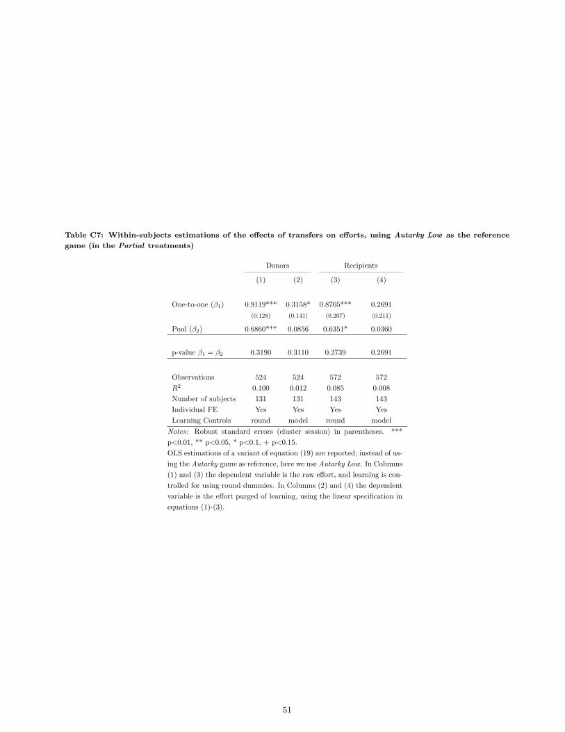
Table C7: Within-subjects estimations of the effects of transfers on efforts, using Autarky Low as the reference

game (in the Partial treatments)

Donors Recipients

(1) (2) (3) (4)

One-to-one (β1) 0.9119*** 0.3158* 0.8705*** 0.2691

(0.128) (0.141) (0.207) (0.211)

Pool (β2) 0.6860*** 0.0856 0.6351* 0.0360

p-value β1 = β2 0.3190 0.3110 0.2739 0.2691

Observations 524 524 572 572

R2 0.100 0.012 0.085 0.008

Number of subjects 131 131 143 143

Individual FE Yes Yes Yes Yes

Learning Controls round model round model

Notes: Robust standard errors (cluster session) in parentheses. ***

p<0.01, ** p<0.05, * p<0.1, + p<0.15.

OLS estimations of a variant of equation (19) are reported; instead of us-

ing the Autarky game as reference, here we use Autarky Low. In Columns

(1) and (3) the dependent variable is the raw effort, and learning is con-

trolled for using round dummies. In Columns (2) and (4) the dependent

variable is the effort purged of learning, using the linear specification in

equations (1)-(3).

51

Table C8: Interaction with individual and household giving patterns

Donors Recipients Donors Recipients

Partial Full Partial Full Partial Full Partial Full

(1) (2) (3) (4) (5) (6) (7) (8)

One-to-one 0.290+ 0.328* 0.0924 -0.105 0.238 0.265 -0.0502 -0.0266

(0.153) (0.167) (0.239) (0.136) (0.176) (0.178) (0.147) (0.110)

Pool 0.148 0.117 -0.149 -0.0115 0.148 0.449* -0.525+ -0.0465

(0.126) (0.214) (0.336) (0.207) (0.142) (0.206) (0.322) (0.165)

Individual giving Household giving

Giving* One to One 0.0553 -0.358* 0.364+ 0.0675 0.131 -0.109 0.520** -0.0830

(0.297) (0.153) (0.210) (0.217) (0.241) (0.170) (0.215) (0.171)

Giving* Pool -0.154 -0.315 0.391 -0.0620 -0.0986 -0.810* 0.946* 0.0159

(0.288) (0.248) (0.411) (0.192) (0.187) (0.413) (0.405) (0.103)

Observations 512 436 556 468 512 436 556 468

R2 0.012 0.013 0.012 0.002 0.012 0.032 0.031 0.001

Number of subjects 128 109 139 117 128 109 139 117

Individual FE Yes Yes Yes Yes Yes Yes Yes Yes

Notes: Robust standard errors (cluster session) in parentheses. *** p<0.01, ** p<0.05, * p<0.1, +

p<0.15.

OLS estimations of a variant of equation (20), are reported, with Autarky being the reference game. The

dependent variable is the effort purged of learning, using the linear specification in equations (1)-(3). In

equation (20) the Full dummy is replaced by a Giving dummy. The value of the Giving dummy depends

on the subject’s answer to the following post-experimental survey questions: During the last year, did

someone in your household give any help in the form of clothes, food, money, ...?, and If yes, who did

give this help?

For the “Individual giving” results, the Giving dummy equals 1 if the subject answered “I did”.

For the “Household giving” results, the Giving dummy equals 1 if the subject answered “Someone else in

the household”.

52

Table C9: Interaction with individual and household receiving patterns

Donors Recipients Donors Recipients

Partial Full Partial Full Partial Full Partial Full

(1) (2) (3) (4) (5) (6) (7) (8)

One-to-one 0.328+ 0.258 0.246 -0.0180 0.206 0.335 0.224 0.0216

(0.177) (0.177) (0.210) (0.0209) (0.159) (0.203) (0.207) (0.102)

Pool 0.0892 -0.0556 0.0756 0.0117 0.0547 0.0668 -0.0950 0.115

(0.186) (0.205) (0.205) (0.101) (0.207) (0.293) (0.176) (0.207)

Individual receiving Household receiving

Receiving* One to One -0.0479 -0.209 0.0953 -0.131 0.302 -0.349+ 0.108 -0.221

(0.276) (0.263) (0.220) (0.354) (0.244) (0.199) (0.273) (0.206)

Receiving* Pool -0.0140 0.521** -0.162 -0.0573 0.0499 -0.176 0.310 -0.343

(0.227) (0.208) (0.394) (0.359) (0.255) (0.340) (0.285) (0.274)

Observations 524 476 572 484 512 464 568 468

R2 0.012 0.016 0.009 0.001 0.015 0.012 0.010 0.007

Number of subjects 131 119 143 121 128 116 142 117

Individual FE Yes Yes Yes Yes Yes Yes Yes Yes

Notes: Robust standard errors (cluster session) in parentheses. *** p<0.01, ** p<0.05, * p<0.1, +

p<0.15.

OLS estimations of a variant of equation (20), are reported, with Autarky being the reference game. The

dependent variable is the effort purged of learning, using the linear specification in equations (1)-(3). In

equation (20) the Full dummy is replaced by a Receiving dummy. The value of the Receiving dummy

depends on the subject’s answer to the following post-experimental survey questions: During the last year,

did someone in your household receive any help in the form of clothes, food, money, ...?, and If yes, who

did receive this help?

For the “Individual receiving” results, the Receiving dummy equals 1 if the subject answered “I did”.

For the “Household receiving” results, the Receiving dummy equals 1 if the subject answered “Someone

else in the household”.

53

Table C10: Donors - Interaction with individual characteristics

Donor Full

(1) (2) (3) (4) (5) (6)

One-to-one 0.419 0.373 0.277 0.228 0.236 0.246

(0.276) (0.360) (0.170) (0.181) (0.186) (0.262)

Pool 0.105 0.0535 0.179 0.0157 0.0411 0.0656

(0.429) (0.387) (0.227) (0.191) (0.200) (0.195)

Ind. characteristic sex age secondary dwelling assets celebrations

Charact* One to One -0.293 -0.00393 -0.104 0.0342 -0.0414 -0.0351

(0.343) (0.00632) (0.218) (0.0771) (0.0592) (0.305)

Charact* Pool -0.105 -0.000809 -0.319 -0.129 -0.0797 -0.0776

(0.421) (0.0130) (0.231) (0.0911) (0.0855) (0.343)

Observations 444 476 476 476 476 476

R2 0.013 0.008 0.012 0.013 0.011 0.008

Number of subjects 111 119 119 119 119 119

Individual FE Yes Yes Yes Yes Yes Yes

Donor Partial

One-to-one -0.0740 0.684 0.601** 0.308* 0.315* 0.355

(0.220) (0.690) (0.199) (0.138) (0.138) (0.302)

Pool -0.265 -0.144 0.235 0.0665 0.0857 0.119

(0.210) (0.438) (0.166) (0.153) (0.154) (0.177)

Ind. characteristic sex age secondary dwelling assets celebrations

Charact* One to One 0.595* -0.00871 -0.593* 0.0397 0.0322 -0.0849

(0.296) (0.0144) (0.261) (0.0341) (0.0597) (0.428)

Charact* Pool 0.593* 0.00543 -0.310 0.0950 -0.00139 -0.0737

(0.276) (0.00815) (0.241) (0.110) (0.0679) (0.261)

Observations 496 524 524 524 524 524

R2 0.025 0.015 0.023 0.014 0.012 0.012

Number of subjects 124 131 131 131 131 131

Individual FE Yes Yes Yes Yes Yes Yes

Notes: Robust standard errors (cluster session) in parentheses. *** p<0.01, ** p<0.05, * p<0.1, +

p<0.15.

OLS estimations of a variant of equation (20), are reported, with Autarky being the reference game.

The dependent variable is the effort purged of learning, using the linear specification in equations

(1)-(3). In equation (20) the Full dummy is replaced by an Individual Characteristics variable (based

on data collected through the post-experimental questionnaire), as follows:

Sex: a dummy variable which equals 1 if the individual is a woman. Age: the individual’s age

in years. Secondary: a dummy variable which equals 1 if the individual has completed secondary

education. Dwelling: dwelling index, calculated using the principal components analysis on dummy

variables for whether the participant or her family owns their home, availability of running water,

toilet, electricity and dirt floor, the number of rooms and light bulbs. Assets: asset index, calculated

using the principal components analysis using dummy variables for whether the household owns other

real estate properties or land, vehicles, TV, radio, cellphone, gas stove, small kitchen appliances,

refrigerator, washing machine, books; productive assets like agricultural machinery or animals; and

small livestock. Celebrations: a dummy variable which equals 1 the individual reports participating

in community celebrations.

54

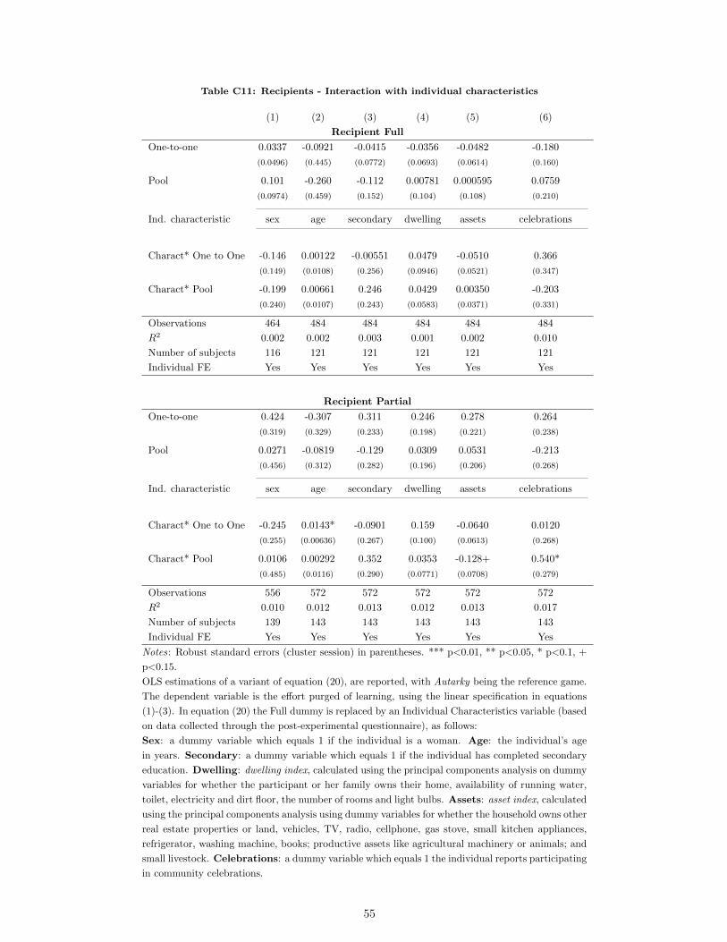
Table C11: Recipients - Interaction with individual characteristics

(1) (2) (3) (4) (5) (6)

Recipient Full

One-to-one 0.0337 -0.0921 -0.0415 -0.0356 -0.0482 -0.180

(0.0496) (0.445) (0.0772) (0.0693) (0.0614) (0.160)

Pool 0.101 -0.260 -0.112 0.00781 0.000595 0.0759

(0.0974) (0.459) (0.152) (0.104) (0.108) (0.210)

Ind. characteristic sex age secondary dwelling assets celebrations

Charact* One to One -0.146 0.00122 -0.00551 0.0479 -0.0510 0.366

(0.149) (0.0108) (0.256) (0.0946) (0.0521) (0.347)

Charact* Pool -0.199 0.00661 0.246 0.0429 0.00350 -0.203

(0.240) (0.0107) (0.243) (0.0583) (0.0371) (0.331)

Observations 464 484 484 484 484 484

R2 0.002 0.002 0.003 0.001 0.002 0.010

Number of subjects 116 121 121 121 121 121

Individual FE Yes Yes Yes Yes Yes Yes

Recipient Partial

One-to-one 0.424 -0.307 0.311 0.246 0.278 0.264

(0.319) (0.329) (0.233) (0.198) (0.221) (0.238)

Pool 0.0271 -0.0819 -0.129 0.0309 0.0531 -0.213

(0.456) (0.312) (0.282) (0.196) (0.206) (0.268)

Ind. characteristic sex age secondary dwelling assets celebrations

Charact* One to One -0.245 0.0143* -0.0901 0.159 -0.0640 0.0120

(0.255) (0.00636) (0.267) (0.100) (0.0613) (0.268)

Charact* Pool 0.0106 0.00292 0.352 0.0353 -0.128+ 0.540*

(0.485) (0.0116) (0.290) (0.0771) (0.0708) (0.279)

Observations 556 572 572 572 572 572

R2 0.010 0.012 0.013 0.012 0.013 0.017

Number of subjects 139 143 143 143 143 143

Individual FE Yes Yes Yes Yes Yes Yes

Notes: Robust standard errors (cluster session) in parentheses. *** p<0.01, ** p<0.05, * p<0.1, +

p<0.15.

OLS estimations of a variant of equation (20), are reported, with Autarky being the reference game.

The dependent variable is the effort purged of learning, using the linear specification in equations

(1)-(3). In equation (20) the Full dummy is replaced by an Individual Characteristics variable (based

on data collected through the post-experimental questionnaire), as follows:

Sex: a dummy variable which equals 1 if the individual is a woman. Age: the individual’s age

in years. Secondary: a dummy variable which equals 1 if the individual has completed secondary

education. Dwelling: dwelling index, calculated using the principal components analysis on dummy

variables for whether the participant or her family owns their home, availability of running water,

toilet, electricity and dirt floor, the number of rooms and light bulbs. Assets: asset index, calculated

using the principal components analysis using dummy variables for whether the household owns other

real estate properties or land, vehicles, TV, radio, cellphone, gas stove, small kitchen appliances,

refrigerator, washing machine, books; productive assets like agricultural machinery or animals; and

small livestock. Celebrations: a dummy variable which equals 1 the individual reports participating

in community celebrations.

55

Table C12: Interaction with locality characteristics

(1) (2) (3) (4) (5) (6) (7) (8)

Donors

Partial Full

One-to-one 0.123 0.597*** 0.174 0.313 0.491* -1.391 0.615 0.587

(0.218) (0.0594) (0.505) (0.807) (0.216) (1.046) (0.472) (0.446)

Pool -0.134 0.302** -1.138+ -0.928 0.200 0.238 0.394 0.229

(0.252) (0.0941) (0.597) (0.966) (0.186) (0.981) (0.304) (0.402)

Location characteristic Share Marginality Share Relig. homoegeneity Share Marginality Share Relig. homoegeneity

Indigenous index Catholic index Indigenous index Catholic index

Locality* One to one 0.286 1.726*** 0.0915 -0.180 -0.376+ -6.111 -0.452 -0.443

(0.344) (0.446) (1.036) (1.899) (0.223) (4.059) (0.574) (0.576)

Locality * Pool 0.434 1.298** 2.007* 1.984 -0.246 0.544 -0.464 -0.234

(0.333) (0.527) (1.014) (1.911) (0.305) (4.034) (0.363) (0.488)

Observations 476 476 476 476 524 524 524 524

R2 0.015 0.020 0.025 0.015 0.017 0.014 0.015 0.013

Number of subjects 119 119 119 119 131 131 131 131

Individual FE Yes Yes Yes Yes Yes Yes Yes Yes

Recipients

Partial Full

One-to-one -0.0836 -0.0213 -0.454*** -0.539*** 0.192 2.269 -0.457 -0.458

(0.0974) (0.0261) (0.0653) (0.0928) (0.263) (3.216) (0.468) (0.509)

Pool 0.0696 -0.244*** -0.117 0.109 0.0502 0.971 0.00623 -0.0157

(0.136) (0.0304) (0.247) (0.356) (0.0871) (3.788) (0.344) (0.451)

Location characteristic Share Marginality Share Relig. homoegeneity Share Marginality Share Relig. homoegeneity

Indigenous index Catholic index Indigenous index Catholic index

Locality* One to One 0.0905 0.107 0.690*** 0.999*** 0.167 7.163 1.110 1.205

(0.107) (0.196) (0.139) (0.229) (0.422) (11.34) (0.718) (0.900)

Locality* Pool -0.158 -1.155*** 0.198 -0.219 -0.0307 3.348 0.0455 0.0858

(0.210) (0.263) (0.509) (0.779) (0.412) (13.18) (0.673) (0.862)

Observations 484 484 484 484 572 572 572 572

R2 0.002 0.006 0.003 0.003 0.009 0.010 0.018 0.018

Number of subjects 121 121 121 121 143 143 143 143

Individual FE Yes Yes Yes Yes Yes Yes Yes Yes

Notes: Robust standard errors (cluster session) in parentheses. *** p<0.01, ** p<0.05, * p<0.1, + p<0.15.

OLS estimations of a variant of equation (20), are reported, with Autarky being the reference game. The dependent variable is the effort purged

of learning, using the linear specification in equations (1)-(3). In equation (20) the Full dummy is replaced by a Locality Characteristic variable

(based on Census data at the municipality level), where Marginality is the Social Backwardness index (SBI) (see Table B2), and the Religious

homogeneity index is defined in Table B1.

56

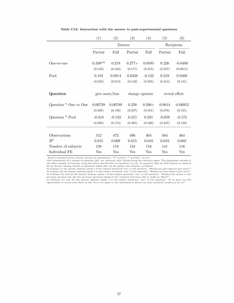
Table C13: Interaction with the answer to post-experimental questions

(1) (2) (3) (4) (5) (6)

Donors Recipients

Partial Full Partial Full Partial Full

One-to-one 0.338** 0.219 0.277+ 0.0585 0.226 -0.0408

(0.123) (0.164) (0.171) (0.215) (0.257) (0.0614)

Pool 0.182 0.0814 0.0328 -0.132 0.219 0.0400

(0.233) (0.213) (0.142) (0.305) (0.214) (0.141)

Question give more/less change opinion reveal effort

Question * One to One 0.00739 0.00789 0.228 0.296+ 0.0814 -0.00952

(0.288) (0.156) (0.237) (0.161) (0.276) (0.121)

Question * Pool -0.218 -0.133 0.215 0.291 -0.659 -0.175

(0.395) (0.174) (0.385) (0.420) (0.447) (0.128)

Observations 512 472 496 464 564 464

R2 0.015 0.009 0.015 0.010 0.019 0.002

Number of subjects 128 118 124 116 141 116

Individual FE Yes Yes Yes Yes Yes Yes

Robust standard errors (cluster session) in parentheses: *** p<0.01, ** p<0.05, * p<0.1.

OLS estimations of a variant of equation (20), are reported, with Autarky being the reference game. The dependent variable is

the effort purged of learning, using the linear specification in equations (1)-(3). In equation (20) the Full dummy is replaced

by an Answer dummy (based on questions asked after all the games were played), as follows:

In Column (1) the Answer dummy equals 1 if the subject answered “yes” to the question: “Would you have liked to give more?”

In Column (2) the Answer dummy equals 1 if the subject answered “yes” to the question: “Would you have liked to give less?”.

In Columns (3) and (4) the Answer dummy equals 1 if the subject answered “yes” to the question: “Would your answer to the

previous question [see the two previous question] change if the recipient had been able to make an effort?”.

In Columns (5) and (6) the Answer dummy equals 1 if the subject answered “yes” to the question: “If we gave you the

opportunity to reveal your effort in the One-to-one game to the individual to whom you were matched, would you do so?”

57

Figures

Game StatePayofftoActive

PayofftoPassive Game StatePayofftoActive

PayofftoPassive

100+75 100+75

100 100

100+75-25 50+25 100+75-75 25+75

100 50 100 25

100+75-25 50+ns(25/n)+25/n 100+75-75 25+ns(75/n)+75/n

100 50+ns(25/n) 100 25+ns(75/n)

100+50 100+75-75 25+ns(75/n)+75/n

100 100 25+ns(75/n)

100+75 25+75

100 25

100+75 200 25+75 175

100+25 200-25 25+75 175-75

100+75 200-nf(25/n) 25+75 175

100+25 200-nf(25/n)-25/n 25+75 175-nf(75/n)-75/n

100+50 25+75 175

100 25+75 175-nf(75/n)-75/n

Post-experimentalquestions Post-experimentalquestions

Questionnaire Questionnaire

One-to-One Pool Public Public

Incentivizedabilitytest2 Incentivizedabilitytest2

AutarkyLow Autarky Pool One-to-One

Pool One-to-One One-to-One Pool

GameordersusedinthePartialtreatments GameordersusedintheFulltreatments

Incentivizedabilitytest1 Incentivizedabilitytest1

Autarky Autarkylow Autarky Autarky

RPOne-to-One RFOne-to-One

RPPool RFPool

RPAutLow RFPublic

DPPool DFPool

DPAutLow DFPublic

RPAutarky RFAutarky

PayoffsinthePartialtreatments PayoffsintheFulltreatments

DPAutarky DFAutarky

DPOne-to-One DFOne-to-One

S

F

S

F

S

F

S

F

S

F

S

F

S

F

S

F

F F

S

F

S

F

S

F

F

S

F

S

F

S

F

S

F

F

S

F

S

F

S

F

S

F

S

F

S

F

S

F

S

F

S

F

F F

Figure 1: The top four boxes show the payoff consequences of the active subject’s effort in the games played by subjects in the

Donor Partial (DP) games, the Donor Full (DF) games, the Recipient Partial (RP) games, and the Recipient Full (RF) games.

In each cell, the first number is the initial endowment, an italicized number the additional income, and a bold number a transfer.

S denotes success, F failure, n the number of passive subjects, ns the number of active subjects other than the subject at hand

who succeeded, and nf the number of active subjects other than the subject at hand who succeeded. The bottom two boxes show

the session structures. Two alternative game orders were used in the Partial treatments (left column) and two alternative game

orders were used in the Full treatments (right column). The order highlighted in dark grey is Order A, and the one highlighted in

lighter grey is Order B.

58

!

!!

!

!

!

!

!

#

#

##

#

#

#

#

Pucnachen

San Agustín (Chunhuas)

Katab

Xculoc

San Antonio Yacasay

Casanayab

San José Carpizo 2

Villamar

San Nicolas

Concepcion

Gral. Ortiz Avila

Moquel

Chunkanan

Xkeulil

Dzitnup

A. Lopez Mateos (La Desconfianza)

²

0 20 40 60 8010

Miles

Tabasco

Yucatan

Quintana Roo

Gulf of Mexico

Guatemala

# Full transfer protocol

! Partial transfer protocol

Main roads South villages

North villages

Figure 2: Map of selected localities and treatment allocation.

Panel A : Donors

Selfish Altruist Warm glow

One-to-One eo1,D < eA eα1,D ≷ eA eγ1,D ≷ eA

Pool eon,D = eo1,D eαn,D ≷ eα1,D eγn,D = eγ1,DPanel B : Recipients

Selfish Altruist Warm glow

One-to-One eo1,R < eA eα1,R < eA eγ1,R ≷ eA

Pool eon,R = eo1,R eαn,R ≷ eα1,R eγn,R = eγ1,RPanel C : Donors vs. Recipients

Selfish Altruist Warm glow

One-to-One

Partial eo1,D(P ) > eo1,R(P ) eα1,D(P ) > eα1,R(P ) eγ1,D(P ) > eγ1,R(P )

Full eo1,D(F ) = eo1,R(F ) eα1,D(F ) > eα1,R(F ) eγ1,D(P ) = eγ1,R(P )

Note: ePreferencesGame,Treatment denotes effort of an individual whose preferences are Selfish (o), Altruistic (α), or Warm Glow (γ),

in the game Autarky (A), One-to-One (1), or Pool (n), in the treatment Donor (D), or Recipient (R). When information

about Partial (P ) and Full (F ) is absent, it means that the result applies to both.

Figure 3: Theoretical predictions.

59

PartialFigure2 04/07/18 12:06

45

67

8Nu

mbe

r of n

uts

thre

aded

Order A Order B Order A Order B

Recipients

Donors

Ability test 1 Autarky highAutarky low Pool transferOne-to-One transfer Ability test 2

Partial

fullfigure2 07/07/18 14:49

45

67

8Nu

mbe

r of n

uts

thre

aded

Order A Order B Order A Order B

Recipients

Donors

Ability test 1 Autarky highOne-to-One transfer Pool transferPublic good transfer Ability test 2

Full

Figure 4: Raw levels of effort in the ability tests and the experimental games.

Figure 5: U(ei, e) for e = 0.2

ability1 04/07/18 14:49

0.0

5.1

.15

.2.2

5Ef

fort

abilit

y te

st 1

0 5 10 15x

Recipient partial Recipient fullDonor partial Donor full

Distribution First Ability Test - Role and protocol

ability2 07/07/18 11:12

0.0

5.1

.15

.2.2

5Ef

fort

abilit

y te

st 1

0 5 10 15x

Order A partial Order B partialOrder A full Order B full

Distribution First Ability Test - Orders

Figure 6: Effort distributions in the first ability test, for different treatments and roles, and for the different orders.

60

PDlearn 07/07/18 11:49

55.

56

6.5

77.

5ef

fort

1 2 3 4 1 2 3 4

Order A

Order B

predicted raw

Partial Donors

Graph 07/07/18 11:40

5.5

66.

57

7.5

effo

rt

1 2 3 4 1 2 3 4

Order A

Order B

predicted raw

Partial Recipients

Figure 7: The figure shows the raw and the predicted levels of effort (as per equation (2)) across roles (donor and recipients) for

the autarky and transfer games in the Partial treatments. The orders are: (A) Autarky, Autarky Low, Pool, One-to-one, and (B)

Autarky Low, Autarky, One-to-one, Pool. Predicted and raw effort coincide in the first round by construction.

Graph 07/07/18 13:49

5.5

66.

57

7.5

8ef

fort

1 2 3 4 1 2 3 4

Order A

Order B

predicted raw

Full Donors

Graph 07/07/18 13:47

5.5

66.

57

7.5

effo

rt

1 2 3 4 1 2 3 4

Order A

Order B

predicted raw

Full Recipients

Figure 8: The figure shows the raw and the predicted levels of effort (as per equation (2)) across roles (donor and recipients) for

the autarky and transfer games in the Full treatments. The orders are: (A) Autarky, Pool, One-to-one, Public and (B) Autarky,

One-to-one, Pool, Public. Predicted and raw effort coincide in the first round by construction.

61