Do High-Wage Jobs Attract more Applicants?

Directed Search Evidence

from the Online Labor Market∗

Stefano Banfi† Benjamın Villena-Roldan‡

Chilean Ministry of Energy

University of Chile, Department of Industrial Engineering,

Center for Applied Economics

January 29, 2018

Abstract

Labor markets become more efficient in theory if jobseekers direct their search. Us-

ing online job board data, we show that high-wage ads attract more applicants as in

directed search models. Due to distinctive data features, we also estimate significant

but milder directed search for hidden (or implicit) wages, suggesting that ad texts and

requirements tacitly convey wage information. Since explicit-wage ads often target un-

skilled workers, other estimates in the literature ignoring hidden-wage ads may suffer

from selection bias. Moreover, job ad requirements are aligned with their applicants’

traits, as predicted in directed search models with heterogeneity.

Keywords: directed search, wage posting, online job board, segmentation.

JEL codes: J64, J22, J42, E24.

∗We thank Sekyu Choi, Andrew Davis, Elton Dusha, Felipe Balmaceda, Guido Menzio, Christian Holzner, Philipp Kircher, RandyWright, Mike Elsby, Brian Tavares, David Wiczer, Alexander Monge, Richard Mansfield, Jennifer Klein, Maximiliano Dvorkin, JoseMustre-del-Rio, Jon Willis, Marianna Kudlyak, Toshihiko Mukoyama, Robert Hall, Kory Kroft, Sofia Bauducco, and Alvaro Aguirre foradvice and discussions at several stages of this project. We also thank participants at presentations at the St. Louis Fed, 2016 AEAMeeting, 2015 Santiago Search & Matching Meeting, Kansas City Fed, 2015 Fall Midwest Macro Meeting, Chilean Economic Society,Central Bank of Chile, and the 2015 Annual SaM Meeting. Villena-Roldan thanks for financial support the FONDECYT project 1151479,Proyecto CONICYT PIA SOC 1402, and the Institute for Research in Market Imperfections and Public Policy, ICM IS130002, Ministeriode Economıa, Fomento y Turismo de Chile. Banfi thanks scholarship CONICYT-Magister Nacional year 2013-22130110. We are indebtedto www.trabajando.com for providing the data, and especially to Ignacio Brunner and Alvaro Vargas for valuable practical insightsregarding the data structure and labor market behavior.

†sbanfi@minenergia.cl.‡Corresponding author: bvillena@dii.uchile.cl

1

1 Introduction

Nowadays workers routinely search for job ads on websites such as www.monster.com in the

US, or www.trabajando.com in several countries, including Chile and other Latin American

countries. Applicants consider wages and other features posted in job ads to direct their

search effort. On the other side, employers post to attract the appropriate kind and number

of applications. Theoretical models of the labor market in the search and matching tradition

typically propose a precise way in which workers seek jobs or employers seek and select

applicants. With few exceptions, existing models advocate either random search, in which

wages are determined ex post in a bargaining setting and play no role in driving applications,

or directed search, in which wages do drive applications and impact the probabilities of

obtaining positions.

Researchers often pick random or directed search based on analytical convenience and

theoretical implications rather than the alignment between theory and evidence. However,

characterizing deep underlying behavior matters for prescribing policies in counterfactual

scenarios. Since it is often possible to construct models generating similar predictions based

on different premises, evaluating competing models based solely on indirect empirical impli-

cations is often insufficient.

The prevalence of random or directed search in frictional markets implies different norma-

tive policy implications. Job search efforts negatively impact the matching chances of others

on the same side of the market, and positively affect the chances of those on the opposite

side in a frictional market. In the simplest case with homogeneous agents, Hosios (1990)

shows that random search with ex post wage bargaining yields inefficient outcomes in the

labor market unless the vacancy-elasticity of the matching function equals the firm bargain-

ing power. Workers and employers do not internalize the externalities they generate when

bargaining over the surplus in a bilateral monopoly situation.

In contrast, under directed search, jobseekers have information about specific job offers

and apply more to positions with higher announced wages (Moen 1997) or target the submar-

ket where employers open positions with specific requirements and announce optimally de-

signed take-it-or-leave-it wage schedules (Menzio and Shi 2010; Menzio et al. 2016). Since

these models predict a unique (sub)market equilibrium wage, an observed cross-sectional

positive correlation between wages and applications would be out of equilibrium. Models

with multiple applications, a sensible assumption in our online context, can solve this tension

because they predict a positive correlation and equilibrium wage dispersion as a consequence

of the strategic behavior of applicants and employers (Albrecht et al. 2006; Galenianos and

2

Kircher 2009; Kircher 2009). Moreover, unobserved heterogeneity in both sides of the mar-

ket could also be a reason for coexistence of wage dispersion and directed search behavior.

A recent in-depth survey for directed search is Wright et al. (2017).

In most models, directed search behavior implies constrained efficiency of the labor mar-

ket allocation.1 Intuitively, agents internalize congestion externalities by realizing the trade-

off between the wage and the likelihood of being hired. Thus, labor market regulations may

be welfare-improving under random search, but not under directed search. For instance,

under directed search Moen and Rosen (2004) show that poaching activity does not distort

training decisions. In contrast, Acemoglu (1997) finds that training subsidies increase wel-

fare because poaching induces suboptimal training investment under random search. With

respect to other policies such as minimum wages and unemployment insurance, several pa-

pers show welfare-improving effects under search frictions (Acemoglu and Shimer 2000;

Acemoglu 2001; Flinn 2006).

Hence, empirical evidence on the prevailing type of job search behavior should shape

policy recommendations. However, finding solid evidence for random or directed search is

difficult for at least two reasons. In an ideal experiment for homogeneous jobs, we would

clone job ads except for an exogenously modified offered wage and compare application

responses. Then, we would estimate the average causal impact of wages in applications

received, as in Belot et al. (2015). The potential problems of this approach are aggregate

effects of the intervention and suspicious jobseekers detecting identical ads with different

wages. Instead, to test for directed search behavior, we use proprietary data from the Chilean

job board www.trabajando.com, described in Section 2. The data merges the information

of applicants, firms, applications, and job ads in a context of heterogeneous workers and

positions.

A second challenge is that most employers do not explicitly post wages, and if they do, the

advertised positions are clearly different from those in which wages are not revealed. Sur-

mounting this sample selection issue is important to provide convincing evidence of directed

search because job ads with hidden wages are predominant. Such ads account for 86.6% of

all job ads in www.trabajando.com, 75.2% in www.monster.com (Brencic 2012), 80% in

www.careerbuilder.com (Marinescu and Wolthoff 2015), and 83% in www.zhaopin.com,

a Chinese online job board (Kuhn and Shen 2013). In contrast, we investigate the behavior

of applicants facing offered wages even if employers choose not to show them in the job ad.

1Within the class of multiple application models Kircher (2009) is an example of decentralized constrainedefficiency in contrast to Galenianos and Kircher (2009).

3

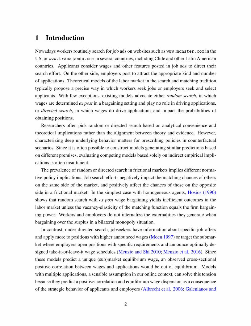
This is due to the job ad form for prospective employers having a mandatory field of “ap-

proximated net monthly wage”2 (Salario lıquido mensual aproximado in Spanish) as shown

in Figure 1. The prospective employer has to enter a single amount representing a monthly

net wage offer. Unlike other websites, entering a wage range is not allowed. However, next

to the wage box employers can choose if they want to make the wage visible to applicants.

This option is selected for only 13.4% of ads in our sample. In Section 2.5, we show that

hidden wages are reliable measures of wages that employers intend to pay. To the best of

our knowledge, this is a unique feature among databases of this sort that allows us to circum-

vent a large sample selection problem when estimating the responsiveness of applications to

wages.

Figure 1: Standard job ad form

Note: Accessed on May 5th, 2015. Red asterisks indicate that the required field is mandatory.

Section 3 shows our results for directed search and wage posting. First, using negative

binomial models for count data allowing for under- or over-dispersion (Cameron and Trivedi

2013) in Section 3.1, we find evidence of directed search in the sense that the number of

applications increases in the offered wage, even if hidden. This impact is significantly larger

for ads in which the wage offer is observable for applicants. Applicants react to hidden2A customary characteristic of the Chilean labor market is that wages are generally expressed in a monthly

rate net of taxes, mandatory contributions to health services (7% of monthly wage), a fully-funded privatepension system (10%), disability insurance (1.2%), and unemployment insurance account (0.6%).

4

wages probably because they use search filters by wage bracket that are fine for low wages

and coarse for large ones. Even within a bracket, as we show below, applicants may infer

wages through information in the job ad. Consequently, we refer to hidden wages as implicit

interchangeably. The evidence suggests that directed search prevails for job seekers in the

online job board, even if wages are not explicit. We thus interpret implicit wage job ads as

noisy signals that attract skilled applicants, perhaps indicating potential ex post bargaining,

as in the Michelacci and Suarez (2006) model. In addition, we also show that job ads posting

low explicit wages receive significantly fewer applications, controlling for job ad features

and firm characteristics.

In the literature few empirical papers show some evidence on application responding posi-

tively to higher wages. We believe we are the first showing this effect for employers not post-

ing explicit wages. Holzer et al. (1991) show that vacancies for which minimum wage regu-

lation is binding provide extra rents that attract more applicants. Dal Bo et al. (2013) find that

higher wages attract more and better qualified applicants in a Mexican public sector online

job board. Marinescu and Wolthoff (2015) use online job ads by www.careerbuilder.com

and explain job ad posted wages mainly through job titles, as we do in our results. They

provide evidence of directed search job ads with explicitly posted wages, which comprise

nearly 20% of their sample, but they are silent about job ads with hidden wages. Belot et al.

(2015) set up a field experiment by altering original posted wages of real job ads. Their

results support the directed search hypothesis, since high-wage jobs receive significantly

more applications than their low-wage experimental clones. Braun et al. (2016) use NLSY

data to estimate duration models and show that search effort is higher in high-wage markets

compared to medium-wage markets. Finally, for product markets Lewis (2011) shows that

internet seekers for used cars react significantly to posted information regarding automobile

quality.

For our second finding, we show that similar workers tend to apply for the same jobs

and their qualifications closely meet employers’ requirements in Section 3.2, as endogenous

segmentation arises in directed search models with heterogeneity on at least one side of the

market (e.g. Shi 2002; Menzio et al. 2016), We also show that wages attract applications

within submarkets defined in various ways in Section 3.3. Therefore, the observed behavior

of applicants is inconsistent with random search within submarkets, a hypothesis competing

with directed search.

In the literature, to the best of our knowledge, only Dal Bo et al. (2013) provide some

evidence interpretable as segmentation since job characteristics such as location and munic-

5

ipality features drive applicant search. In a similar vein, we document jobseekers targeting

ads with requirements that fit their characteristics, regardless of the final hiring decision. Of-

ten weak correlations between worker and firm effects found in matched employer-employee

databases (e.g. Abowd et al. 1999) might mistakenly be taken as segmentation since good

workers match with good jobs as implied by directed search models. However, employ-

ers may also select among multiple randomly sent applications as in non-sequential random

search models (Moen 1999; Villena-Roldan 2012). Hence, these correlations are not neces-

sarily evidence of the segmentation implied by directed search.

Our third empirical fact concerns wage posting behavior, a decision interlinked with ap-

plications in Section 3.4. We find that firms are more likely to post a wage explicitly for

low-skill jobs. This evidence, on top of the negative impact of explicit wage posting in the

number of applicants in Section 3.1, suggests that employers post explicit wages to receive

fewer applications. In this way, they avoid large screening costs, especially for simple jobs

in which differentiation across suitable candidates barely matters. Posting explicit wages is

a strategic decision correlated with factors also affecting offered wages. Hence, studying

directed search behavior only through explicitly posted wages leads to biased evidence. In

fact, given the empirical estimates obtained in Sections 3.1 and 3.4, we conclude that there

is an upward bias in the sensitivity of applications to wages when neglecting the endogenous

decision of posting explicit wages.

In line with our findings, Brencic (2012) shows that explicit wage posting is standard

in job ads requiring low qualifications and those that need to be filled fast. The evidence

suggests that firms face a trade-off when announcing a wage: it reduces search costs, but

decreases the quality of applicants. Due to the link between directed search and committed

explicit wage posting in most models (i.e. competitive search), some authors investigate the

prevalence of wage-posting and wage-bargaining behavior. Brenzel et al. (2014) report a

sizable share of wage posting, often concentrated in low-skill jobs. Hall and Krueger (2012)

report that nearly one-third of workers were largely certain of the wage paid before applying.

However, knowing wages is not a concrete indication of directed search since it may just

reflect anticipation of a bargaining result. All in all, the evidence suggests that implicit wage

posting is frequently used to target skilled workers and that ex post bargaining and directed

search may coexist.

Finally, Section 4 summarizes and concludes that applicants noticeably react to informa-

tion posted (or hidden) in job ads, and employers strategically configure ads to attract or to

hinder targeted groups of workers.

6

2 Data description

Our data covers all job ads posted, all job seekers and all job applications between January

1st, 2008 and June 14th, 2014 for the Chilean job board www.trabajando.com. This job

board operates several websites, generating multiple simultaneous appearances of job ads,

or repetitions of previously posted ads. There are three main databases: the first one has

applications to each job ad and personal data on the applicants; the second one contains

employer information, and the third one gathers information on job ads.

Applicants register for free in the website and fill out a form to provide demographic

information, educational record, previous worker experience, etc. Employers complete the

form in Figure 1 and pay3 USD 116 for a 60-day term posting, as of December 2014. While

www.trabajando.com keeps records of hidden wages, employers may provide nonsensical

information. We keep 6,131,626 applications during the mentioned period, after removing

nearly two million cases with unreliable wage information.4

Jobseekers can filter job ads by job title keywords, region, posting date, occupation, job

ad type, and full/part time arrangement. They can also filter jobs by monthly wage offer level

in ranges as narrow as CLP 100,000 (USD 163) for wages below CLP 1,000,000. For wages

between CLP 1,000,000 and 3,500,000, jobseekers could filter in ranges of CLP 500,000 at

most. Ads with hidden wage are listed in these ranges when filtering by wage offer level.

We have no information regarding the filters jobseekers actually use to find postings because

users are not required to login to search job offers.

2.1 Applicants

Individuals are identified in the database by unique combinations of years of experience, date

of birth, date of entry of the resume, gender, nationality, and profession. Only nine duplicated

cases are dropped.

We keep individuals between 18 to 69 years old with monthly net wages lower than 5 mil-

lion pesos in their previous work (9,745 USD per month, using the average nominal exchange

rate over 2008Q1 - 2014Q2), which is well above the 99th percentile according to CASEN

3The price was CLP 59,900 + 19% of value added tax. Current terms are located at http://www1.trabajando.cl/empresas/noticia.cfm?noticiaid=3877. The cost in dollars is computed using theDecember 2014 average CLP/USD spot exchange rate. The job board also offers preferential rates for bigclients.

4We discuss data cleaning details in the online appendix (OA) in Section A.1.

7

2011, a Chilean household survey akin to the March CPS). We also exclude individuals with

monthly net wage expectations over 5 million pesos, and those who omit an expected figure

in the application form (as econometricians, we observe this expectation even if applicants

choose to hide it from employers). Excluding these cases, we get 463,495 applicants. De-

scriptive statistics are in Tables 1.5

The sample is young (30 years old on average) and mostly single. More than 60% of the

applicants are in the Metropolitan Region of Santiago. The sample shows a high educational

level, so they are likely paid above the legal minimum wage (approximately 377 USD per

month). About 42% of the sample has some kind of college education, and 27% of applicants

have a technical tertiary degree. We estimate schooling according to the highest educational

level achieved (8 years for primary, 12 years for both Scientific-Humanistic or Technical high

school, 16 years for technical tertiary degrees, 17 years for university (college) degrees, and

18 years for graduate degrees). The average schooling is 15 years and is similar for males and

females. Males are more likely to be in technical or technology related areas, while females

are often in sales. A significant share of applicants do not declare an area.

Given the youth of the sample, most individuals have few years of work experience. On

average, individuals possess 6.5 potential years of experience, with males slightly more ex-

perienced. A large proportion of the sample are self-reported as unemployed (47.74%), who

are more likely to be females. The rest of the applicants are on-the-job searchers.

The gender gap in expected wages paid is nearly 44%, similar to the gap of last/current

jobs. Applicants expect to be better off from a job change: expected wages for the next job

are 3.9% higher than their last or current job.6 Applicants’ wage expectations tend to be

private: less than half of the sample chooses to display their wage expectations to employers.

2.2 Employers

Our sample has 6,386 different firms.7 A sizable set of firms have less than 50 employees,

but this figure is affected by recruiting firms that offer their services to contact and select

potential applicants for their clients. We consider a recruiting firm as one posting a number

of vacancies exceeding half of the upper limit of its reported interval of employees in a

5For data cleaning details, see our online appendix (OA), Section A.1. For more descriptive details, see ourOA, Section A.2, Tables A2 and A3.

6Summary statistics of applicant last job wages are reported in the OA, Section A.2, Table A27We describe firm data in greater detail in the OA, Table A4.

8

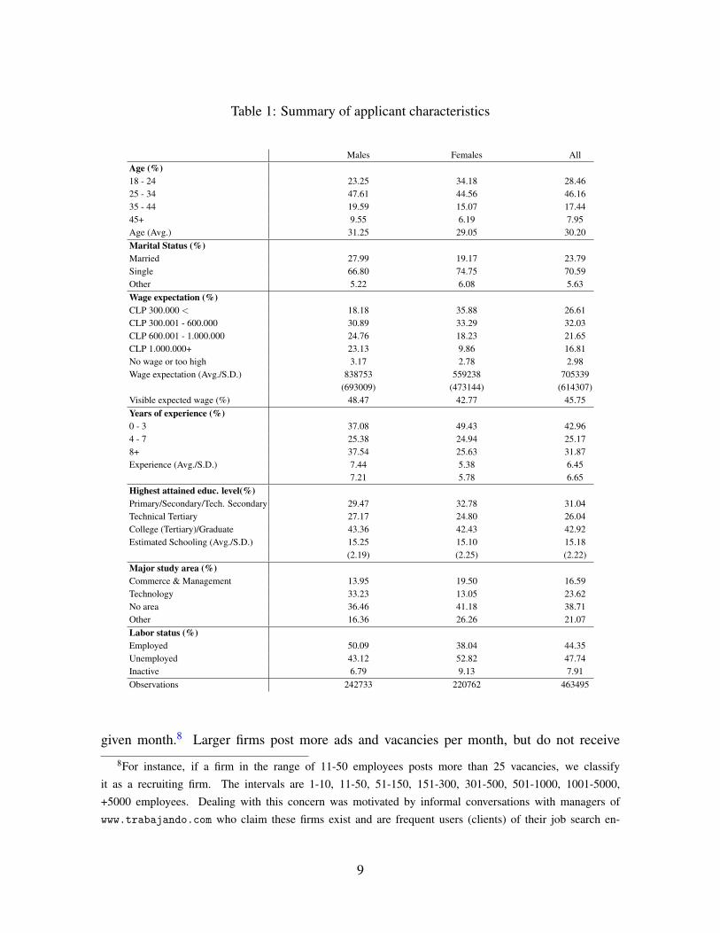
Table 1: Summary of applicant characteristics

Males Females AllAge (%)18 - 24 23.25 34.18 28.4625 - 34 47.61 44.56 46.1635 - 44 19.59 15.07 17.4445+ 9.55 6.19 7.95Age (Avg.) 31.25 29.05 30.20Marital Status (%)Married 27.99 19.17 23.79Single 66.80 74.75 70.59Other 5.22 6.08 5.63Wage expectation (%)CLP 300.000 < 18.18 35.88 26.61CLP 300.001 - 600.000 30.89 33.29 32.03CLP 600.001 - 1.000.000 24.76 18.23 21.65CLP 1.000.000+ 23.13 9.86 16.81No wage or too high 3.17 2.78 2.98Wage expectation (Avg./S.D.) 838753 559238 705339

(693009) (473144) (614307)Visible expected wage (%) 48.47 42.77 45.75Years of experience (%)0 - 3 37.08 49.43 42.964 - 7 25.38 24.94 25.178+ 37.54 25.63 31.87Experience (Avg./S.D.) 7.44 5.38 6.45

7.21 5.78 6.65Highest attained educ. level(%)Primary/Secondary/Tech. Secondary 29.47 32.78 31.04Technical Tertiary 27.17 24.80 26.04College (Tertiary)/Graduate 43.36 42.43 42.92Estimated Schooling (Avg./S.D.) 15.25 15.10 15.18

(2.19) (2.25) (2.22)Major study area (%)Commerce & Management 13.95 19.50 16.59Technology 33.23 13.05 23.62No area 36.46 41.18 38.71Other 16.36 26.26 21.07Labor status (%)Employed 50.09 38.04 44.35Unemployed 43.12 52.82 47.74Inactive 6.79 9.13 7.91Observations 242733 220762 463495

given month.8 Larger firms post more ads and vacancies per month, but do not receive

8For instance, if a firm in the range of 11-50 employees posts more than 25 vacancies, we classifyit as a recruiting firm. The intervals are 1-10, 11-50, 51-150, 151-300, 301-500, 501-1000, 1001-5000,+5000 employees. Dealing with this concern was motivated by informal conversations with managers ofwww.trabajando.com who claim these firms exist and are frequent users (clients) of their job search en-

9

more applicants per ad or vacancy posted. By industry, a majority of firms are in retail,

communications, services, or manufacturing. The posting frequency of ads and vacancies

varies substantially across industries, with the highest values in primary sectors (agriculture,

fishing, and mining) and the lowest in construction and services. However, job seekers apply

more for industries that post fewer ads or vacancies, such as household services, personal

services, and public administration.

2.3 Job Ads

Job ads have requirements for applicants, a number of open positions (vacancies), and an

estimated offered wage, potentially hidden by the employer. Descriptive statistics for job ads

are shown in Table 2.9 Our sample excludes jobs with (i) an estimated offered monthly wage

below CLP 100,000 or over CLP 5,000,000 (USD 194-9,745 approximately); (ii) missing

or unreliable information for offered wages (explicit or hidden); and (iii) a requirement of

experience over 20 years, or a missing experience request. After cleaning, 184,920 job ads

remained in our sample, some of them with missing fields.

In the online labor market data, only 13.4% of job ads post wages explicitly. In Table 2

we see that most job ads require little labor experience, which is even more noticeable for

jobs with explicit wages. The mean and standard deviation of explicit wages is 40% lower

than of implicit ones. Job ads with explicit wages tend to require no specific profession or

occupation, low experience, and high-school education. Explicit-wage ads concentrate in re-

tail, communications, and services. Implicit-wage ads receive substantially more applicants

on average than explicit-wage ones. The average number of applications per ad is 34.8, with

a large dispersion.

2.4 Job Ad Titles

The job title itself may convey relevant information on the set of tasks that a worker would

undertake once hired, the hierarchy in the organization, relevant qualifications, etc. Mari-

nescu and Wolthoff (2015) use job titles from www.careerbuilder.com data to assess their

predictive power on the 20% of job ads that post an explicit wage in their sample. In the

same fashion, we use job titles (in Spanish) of ads posted in www.trabajando.com.

gine. Even though our definition is admittedly ad hoc and it is not immune to potential misclassification, ourresults are barely changed by this issue, as we show below.

9For further details, please see the OA, Section A.2, Tables A5, A6, and A7.

10

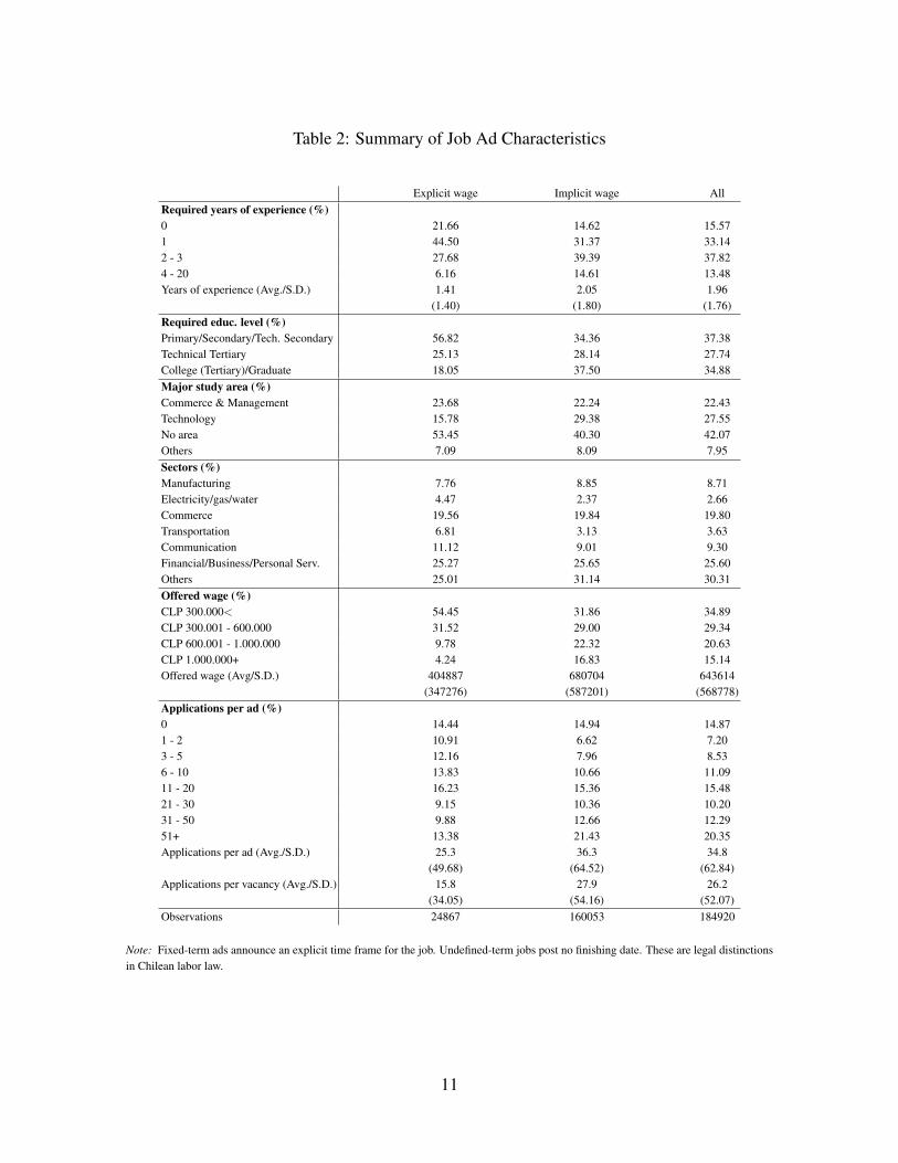
Table 2: Summary of Job Ad Characteristics

Explicit wage Implicit wage AllRequired years of experience (%)0 21.66 14.62 15.571 44.50 31.37 33.142 - 3 27.68 39.39 37.824 - 20 6.16 14.61 13.48Years of experience (Avg./S.D.) 1.41 2.05 1.96

(1.40) (1.80) (1.76)Required educ. level (%)Primary/Secondary/Tech. Secondary 56.82 34.36 37.38Technical Tertiary 25.13 28.14 27.74College (Tertiary)/Graduate 18.05 37.50 34.88Major study area (%)Commerce & Management 23.68 22.24 22.43Technology 15.78 29.38 27.55No area 53.45 40.30 42.07Others 7.09 8.09 7.95Sectors (%)Manufacturing 7.76 8.85 8.71Electricity/gas/water 4.47 2.37 2.66Commerce 19.56 19.84 19.80Transportation 6.81 3.13 3.63Communication 11.12 9.01 9.30Financial/Business/Personal Serv. 25.27 25.65 25.60Others 25.01 31.14 30.31Offered wage (%)CLP 300.000< 54.45 31.86 34.89CLP 300.001 - 600.000 31.52 29.00 29.34CLP 600.001 - 1.000.000 9.78 22.32 20.63CLP 1.000.000+ 4.24 16.83 15.14Offered wage (Avg/S.D.) 404887 680704 643614

(347276) (587201) (568778)Applications per ad (%)0 14.44 14.94 14.871 - 2 10.91 6.62 7.203 - 5 12.16 7.96 8.536 - 10 13.83 10.66 11.0911 - 20 16.23 15.36 15.4821 - 30 9.15 10.36 10.2031 - 50 9.88 12.66 12.2951+ 13.38 21.43 20.35Applications per ad (Avg./S.D.) 25.3 36.3 34.8

(49.68) (64.52) (62.84)Applications per vacancy (Avg./S.D.) 15.8 27.9 26.2

(34.05) (54.16) (52.07)Observations 24867 160053 184920

Note: Fixed-term ads announce an explicit time frame for the job. Undefined-term jobs post no finishing date. These are legal distinctionsin Chilean labor law.

11

Our approach to extract information from job titles is akin to Marinescu and Wolthoff

(2015). We recognize the first four meaningful words of the job title, after deleting articles,

connectors, etc, and construct four categorical variables representing a list of words repeated

more than 100 times in the whole sample of titles, as one of the first four words. Since most

words in Spanish are not gender neutral, we consider male and female words as the same.

This entails some loss of information since the employer could succinctly define a desired

gender for the applicant, a feature employed in the literature (Kuhn and Shen 2013).

The first word has 140 different categories such as: analyst (analista), chief (jefe), man-

ager (administrador), assistant (asistente), engineer (ingeniero), intern (practica), etc. The

second one considers 290 categories, and the third and fourth have 218 and 67 categories, re-

spectively. If a word in the job title does not appear in the selected list, it is denoted as Other.

For the whole sample of job ads, the first word was catalogued as Other only in the 7.04% of

ad titles. 17.22%, 27.33% and 12.68% of job ads were categorized into the Other group for

the second, third, and fourth words, respectively. In Figures A1 and A2 in the Section A.3 of

the OA, we show “word clouds” with the most repeated words for job ads with implicit and

explicit wages, respectively (in Spanish). The larger the word in the cloud, the more repeated

it is in our job title sample. A loose inspection of these word clouds suggests that explicit

wage job ads are more frequent in low skill jobs.

These categorical variables constructed from the job ad titles are used as dummy controls

in the estimations in the models specified in Tables 4 and 8 in the main text, and A8 - A11,

A13 - A16 in the OA.

2.5 Reliability of Implicit Wages

Are employers reliably reporting offered wages when they are choosing not to show them to

applicants? The first reason for employers caring about reporting is that the job board allows

jobseekers to filter by wage ranges, even for implicit wages. Hence, posting nonsensical

information is potentially detrimental for the employer. Moreover, we assess how reliable

implicit wages are by assuming that explicit wages are truthfully reported.

We proceed by estimating a predictive equation for log wages for implicit-wage and

explicit-wage job ads, separately. The baseline explanatory variables are job ad title word,

regional, and quarter binary variables. In augmented models, we incorporate additional re-

gressors in steps, such as experience, education, and 166 different job areas and computer

skill requirements.

The upper panel of Table 3 shows in-sample prediction statistics for regressions by type

12

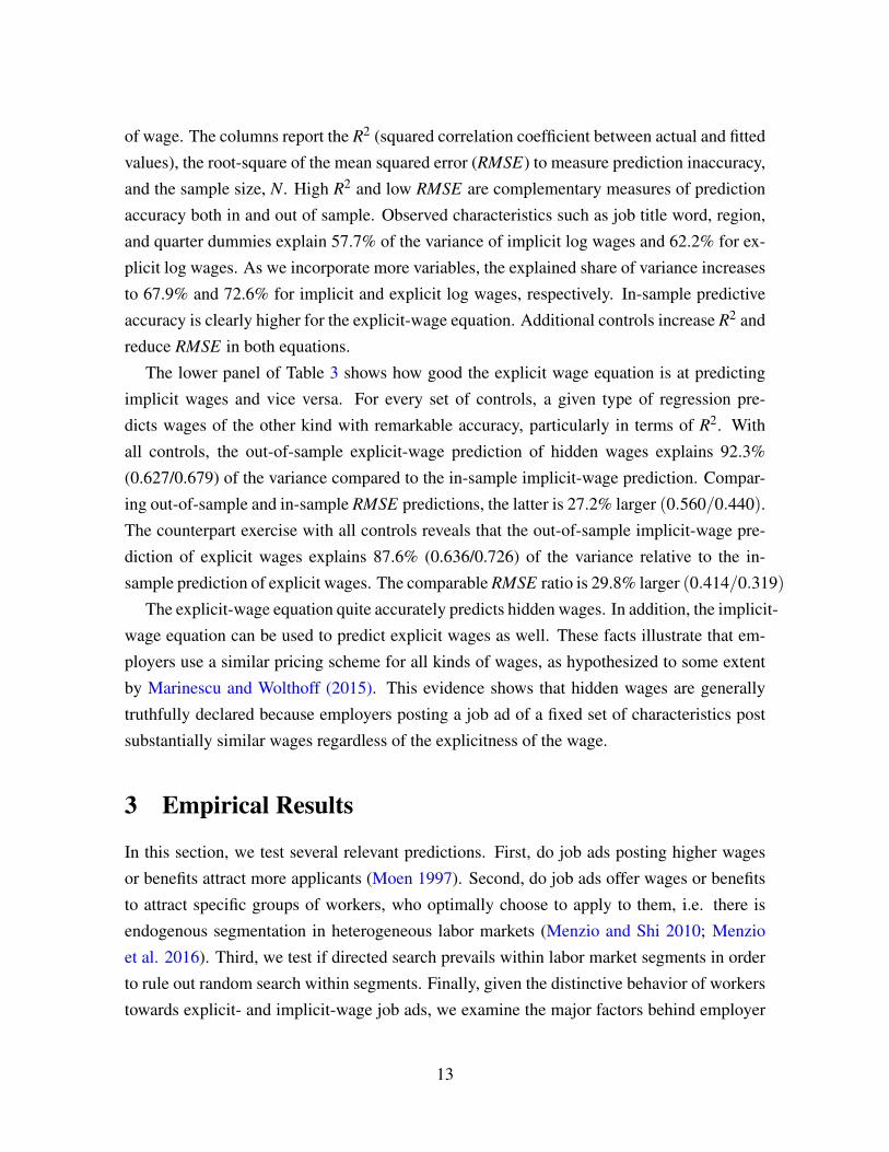
of wage. The columns report the R2 (squared correlation coefficient between actual and fitted

values), the root-square of the mean squared error (RMSE) to measure prediction inaccuracy,

and the sample size, N. High R2 and low RMSE are complementary measures of prediction

accuracy both in and out of sample. Observed characteristics such as job title word, region,

and quarter dummies explain 57.7% of the variance of implicit log wages and 62.2% for ex-

plicit log wages. As we incorporate more variables, the explained share of variance increases

to 67.9% and 72.6% for implicit and explicit log wages, respectively. In-sample predictive

accuracy is clearly higher for the explicit-wage equation. Additional controls increase R2 and

reduce RMSE in both equations.

The lower panel of Table 3 shows how good the explicit wage equation is at predicting

implicit wages and vice versa. For every set of controls, a given type of regression pre-

dicts wages of the other kind with remarkable accuracy, particularly in terms of R2. With

all controls, the out-of-sample explicit-wage prediction of hidden wages explains 92.3%

(0.627/0.679) of the variance compared to the in-sample implicit-wage prediction. Compar-

ing out-of-sample and in-sample RMSE predictions, the latter is 27.2% larger (0.560/0.440).

The counterpart exercise with all controls reveals that the out-of-sample implicit-wage pre-

diction of explicit wages explains 87.6% (0.636/0.726) of the variance relative to the in-

sample prediction of explicit wages. The comparable RMSE ratio is 29.8% larger (0.414/0.319)

The explicit-wage equation quite accurately predicts hidden wages. In addition, the implicit-

wage equation can be used to predict explicit wages as well. These facts illustrate that em-

ployers use a similar pricing scheme for all kinds of wages, as hypothesized to some extent

by Marinescu and Wolthoff (2015). This evidence shows that hidden wages are generally

truthfully declared because employers posting a job ad of a fixed set of characteristics post

substantially similar wages regardless of the explicitness of the wage.

3 Empirical Results

In this section, we test several relevant predictions. First, do job ads posting higher wages

or benefits attract more applicants (Moen 1997). Second, do job ads offer wages or benefits

to attract specific groups of workers, who optimally choose to apply to them, i.e. there is

endogenous segmentation in heterogeneous labor markets (Menzio and Shi 2010; Menzio

et al. 2016). Third, we test if directed search prevails within labor market segments in order

to rule out random search within segments. Finally, given the distinctive behavior of workers

towards explicit- and implicit-wage job ads, we examine the major factors behind employer

13

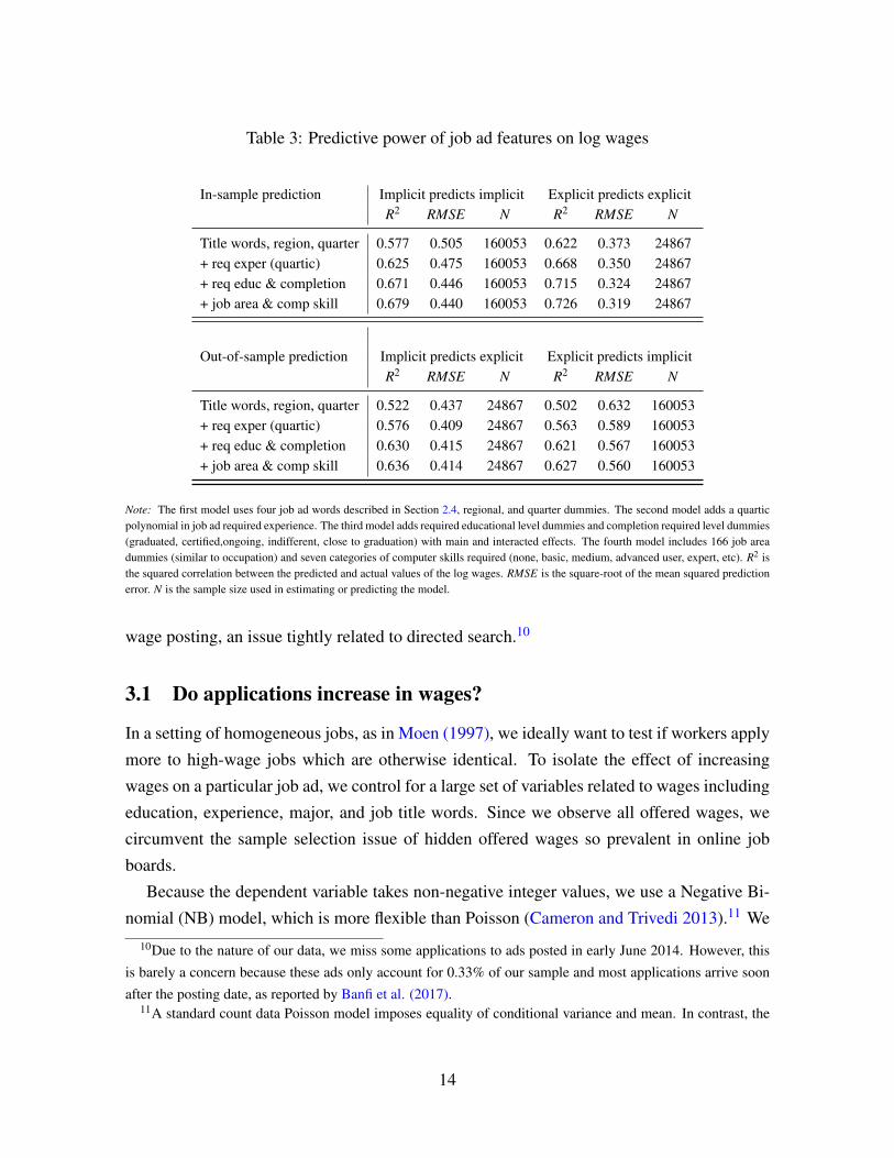
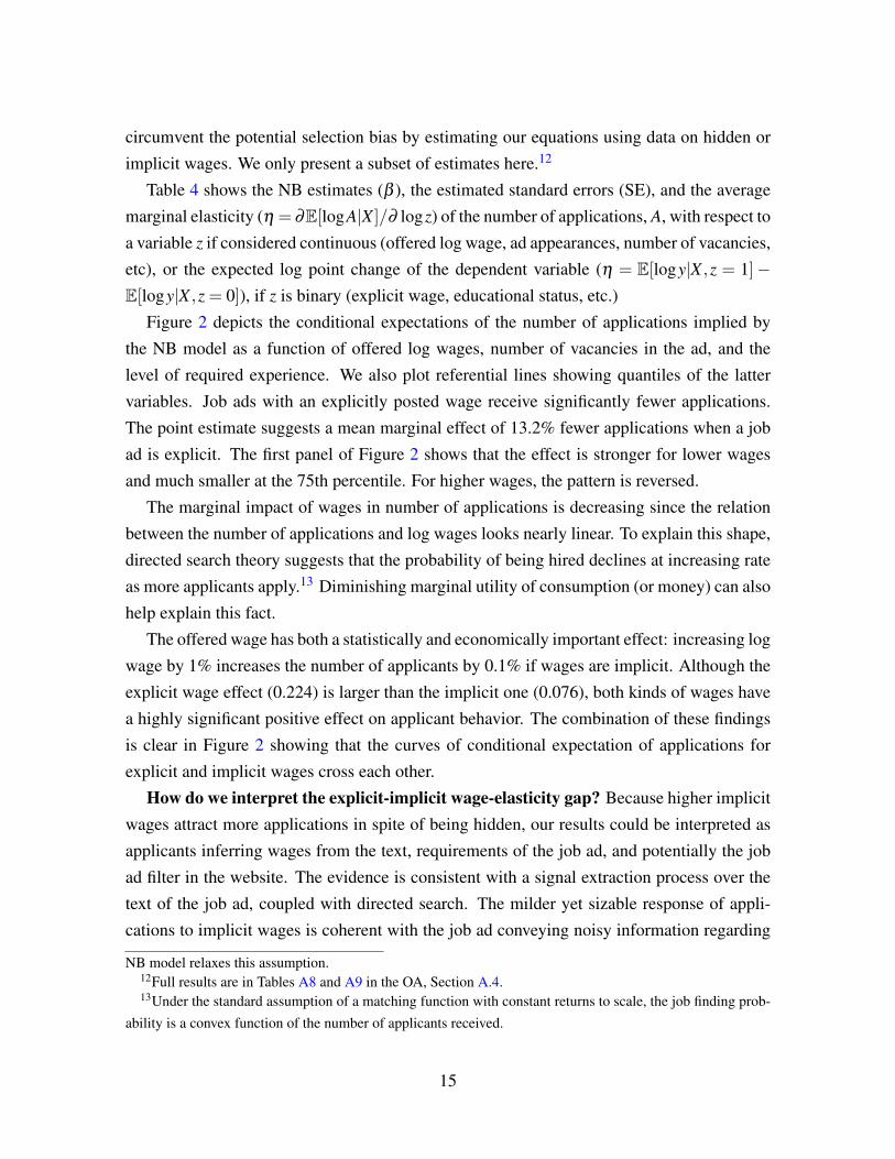
Table 3: Predictive power of job ad features on log wages

In-sample prediction Implicit predicts implicit Explicit predicts explicitR2 RMSE N R2 RMSE N

Title words, region, quarter 0.577 0.505 160053 0.622 0.373 24867+ req exper (quartic) 0.625 0.475 160053 0.668 0.350 24867+ req educ & completion 0.671 0.446 160053 0.715 0.324 24867+ job area & comp skill 0.679 0.440 160053 0.726 0.319 24867

Out-of-sample prediction Implicit predicts explicit Explicit predicts implicitR2 RMSE N R2 RMSE N

Title words, region, quarter 0.522 0.437 24867 0.502 0.632 160053+ req exper (quartic) 0.576 0.409 24867 0.563 0.589 160053+ req educ & completion 0.630 0.415 24867 0.621 0.567 160053+ job area & comp skill 0.636 0.414 24867 0.627 0.560 160053

Note: The first model uses four job ad words described in Section 2.4, regional, and quarter dummies. The second model adds a quarticpolynomial in job ad required experience. The third model adds required educational level dummies and completion required level dummies(graduated, certified,ongoing, indifferent, close to graduation) with main and interacted effects. The fourth model includes 166 job areadummies (similar to occupation) and seven categories of computer skills required (none, basic, medium, advanced user, expert, etc). R2 isthe squared correlation between the predicted and actual values of the log wages. RMSE is the square-root of the mean squared predictionerror. N is the sample size used in estimating or predicting the model.

wage posting, an issue tightly related to directed search.10

3.1 Do applications increase in wages?

In a setting of homogeneous jobs, as in Moen (1997), we ideally want to test if workers apply

more to high-wage jobs which are otherwise identical. To isolate the effect of increasing

wages on a particular job ad, we control for a large set of variables related to wages including

education, experience, major, and job title words. Since we observe all offered wages, we

circumvent the sample selection issue of hidden offered wages so prevalent in online job

boards.

Because the dependent variable takes non-negative integer values, we use a Negative Bi-

nomial (NB) model, which is more flexible than Poisson (Cameron and Trivedi 2013).11 We10Due to the nature of our data, we miss some applications to ads posted in early June 2014. However, this

is barely a concern because these ads only account for 0.33% of our sample and most applications arrive soonafter the posting date, as reported by Banfi et al. (2017).

11A standard count data Poisson model imposes equality of conditional variance and mean. In contrast, the

14

circumvent the potential selection bias by estimating our equations using data on hidden or

implicit wages. We only present a subset of estimates here.12

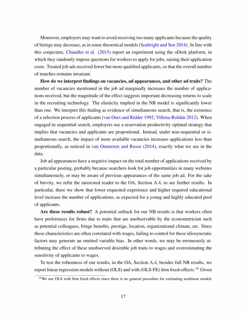
Table 4 shows the NB estimates (β ), the estimated standard errors (SE), and the average

marginal elasticity (η = ∂E[logA|X ]/∂ logz) of the number of applications, A, with respect to

a variable z if considered continuous (offered log wage, ad appearances, number of vacancies,

etc), or the expected log point change of the dependent variable (η = E[logy|X ,z = 1]−E[logy|X ,z = 0]), if z is binary (explicit wage, educational status, etc.)

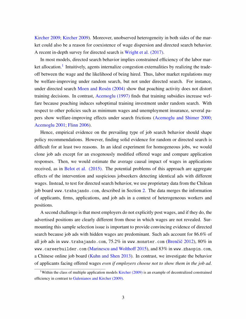
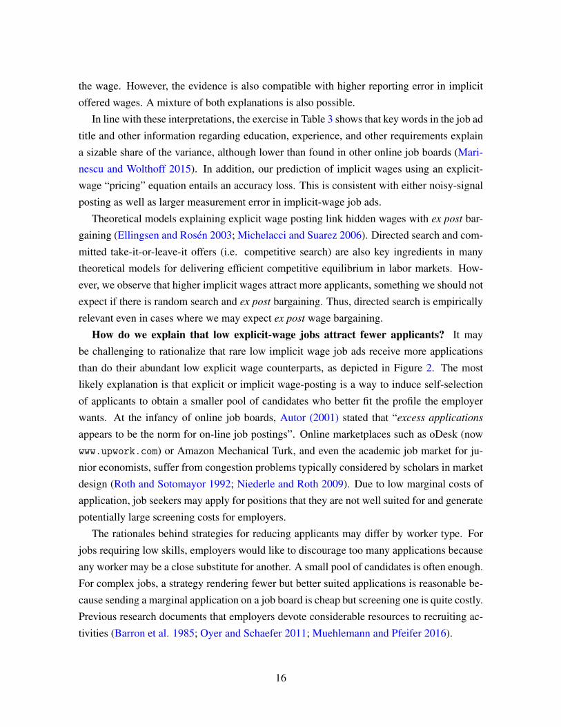
Figure 2 depicts the conditional expectations of the number of applications implied by

the NB model as a function of offered log wages, number of vacancies in the ad, and the

level of required experience. We also plot referential lines showing quantiles of the latter

variables. Job ads with an explicitly posted wage receive significantly fewer applications.

The point estimate suggests a mean marginal effect of 13.2% fewer applications when a job

ad is explicit. The first panel of Figure 2 shows that the effect is stronger for lower wages

and much smaller at the 75th percentile. For higher wages, the pattern is reversed.

The marginal impact of wages in number of applications is decreasing since the relation

between the number of applications and log wages looks nearly linear. To explain this shape,

directed search theory suggests that the probability of being hired declines at increasing rate

as more applicants apply.13 Diminishing marginal utility of consumption (or money) can also

help explain this fact.

The offered wage has both a statistically and economically important effect: increasing log

wage by 1% increases the number of applicants by 0.1% if wages are implicit. Although the

explicit wage effect (0.224) is larger than the implicit one (0.076), both kinds of wages have

a highly significant positive effect on applicant behavior. The combination of these findings

is clear in Figure 2 showing that the curves of conditional expectation of applications for

explicit and implicit wages cross each other.

How do we interpret the explicit-implicit wage-elasticity gap? Because higher implicit

wages attract more applications in spite of being hidden, our results could be interpreted as

applicants inferring wages from the text, requirements of the job ad, and potentially the job

ad filter in the website. The evidence is consistent with a signal extraction process over the

text of the job ad, coupled with directed search. The milder yet sizable response of appli-

cations to implicit wages is coherent with the job ad conveying noisy information regarding

NB model relaxes this assumption.12Full results are in Tables A8 and A9 in the OA, Section A.4.13Under the standard assumption of a matching function with constant returns to scale, the job finding prob-

ability is a convex function of the number of applicants received.

15

the wage. However, the evidence is also compatible with higher reporting error in implicit

offered wages. A mixture of both explanations is also possible.

In line with these interpretations, the exercise in Table 3 shows that key words in the job ad

title and other information regarding education, experience, and other requirements explain

a sizable share of the variance, although lower than found in other online job boards (Mari-

nescu and Wolthoff 2015). In addition, our prediction of implicit wages using an explicit-

wage “pricing” equation entails an accuracy loss. This is consistent with either noisy-signal

posting as well as larger measurement error in implicit-wage job ads.

Theoretical models explaining explicit wage posting link hidden wages with ex post bar-

gaining (Ellingsen and Rosen 2003; Michelacci and Suarez 2006). Directed search and com-

mitted take-it-or-leave-it offers (i.e. competitive search) are also key ingredients in many

theoretical models for delivering efficient competitive equilibrium in labor markets. How-

ever, we observe that higher implicit wages attract more applicants, something we should not

expect if there is random search and ex post bargaining. Thus, directed search is empirically

relevant even in cases where we may expect ex post wage bargaining.

How do we explain that low explicit-wage jobs attract fewer applicants? It may

be challenging to rationalize that rare low implicit wage job ads receive more applications

than do their abundant low explicit wage counterparts, as depicted in Figure 2. The most

likely explanation is that explicit or implicit wage-posting is a way to induce self-selection

of applicants to obtain a smaller pool of candidates who better fit the profile the employer

wants. At the infancy of online job boards, Autor (2001) stated that “excess applications

appears to be the norm for on-line job postings”. Online marketplaces such as oDesk (now

www.upwork.com) or Amazon Mechanical Turk, and even the academic job market for ju-

nior economists, suffer from congestion problems typically considered by scholars in market

design (Roth and Sotomayor 1992; Niederle and Roth 2009). Due to low marginal costs of

application, job seekers may apply for positions that they are not well suited for and generate

potentially large screening costs for employers.

The rationales behind strategies for reducing applicants may differ by worker type. For

jobs requiring low skills, employers would like to discourage too many applications because

any worker may be a close substitute for another. A small pool of candidates is often enough.

For complex jobs, a strategy rendering fewer but better suited applications is reasonable be-

cause sending a marginal application on a job board is cheap but screening one is quite costly.

Previous research documents that employers devote considerable resources to recruiting ac-

tivities (Barron et al. 1985; Oyer and Schaefer 2011; Muehlemann and Pfeifer 2016).

16

Moreover, employers may want to avoid receiving too many applicants because the quality

of hirings may decrease, as in some theoretical models (Seabright and Sen 2014). In line with

this conjecture, Chandler et al. (2015) report an experiment using the oDesk platform, in

which they randomly impose questions for workers to apply for jobs, raising their application

costs. Treated job ads received fewer but more qualified applicants, so that the overall number

of matches remains invariant.

How do we interpret findings on vacancies, ad appearances, and other ad traits? The

number of vacancies mentioned in the job ad marginally increases the number of applica-

tions received, but the magnitude of the effect suggests important decreasing returns to scale

in the recruiting technology. The elasticity implied in the NB model is significantly lower

than one. We interpret this finding as evidence of simultaneous search, that is, the existence

of a selection process of applicants (van Ours and Ridder 1992; Villena-Roldan 2012). When

engaged in sequential search, employers use a reservation productivity optimal strategy that

implies that vacancies and applicants are proportional. Instead, under non-sequential or si-

multaneous search, the impact of more available vacancies increases applications less than

proportionally, as noticed in van Ommeren and Russo (2014), exactly what we see in the

data.

Job ad appearances have a negative impact on the total number of applications received by

a particular posting, probably because searchers look for job opportunities in many websites

simultaneously, or may be aware of previous appearances of the same job ad. For the sake

of brevity, we refer the interested reader to the OA, Section A.4, to see further results. In

particular, there we show that lower requested experience and higher required educational

level increase the number of applications, as expected for a young and highly educated pool

of applicants.

Are these results robust? A potential setback for our NB results is that workers often

have preferences for firms due to traits that are unobservable by the econometrician such

as potential colleagues, fringe benefits, prestige, location, organizational climate, etc. Since

these characteristics are often correlated with wages, failing to control for these idiosyncratic

factors may generate an omitted variable bias. In other words, we may be erroneously at-

tributing the effect of these unobserved desirable job traits to wages and overestimating the

sensitivity of applicants to wages.

To test the robustness of our results, in the OA, Section A.4, besides full NB results, we

report linear regression models without (OLS) and with (OLS-FE) firm fixed-effects.14 Given

14We use OLS with firm fixed effects since there is no general procedure for estimating nonlinear models

17

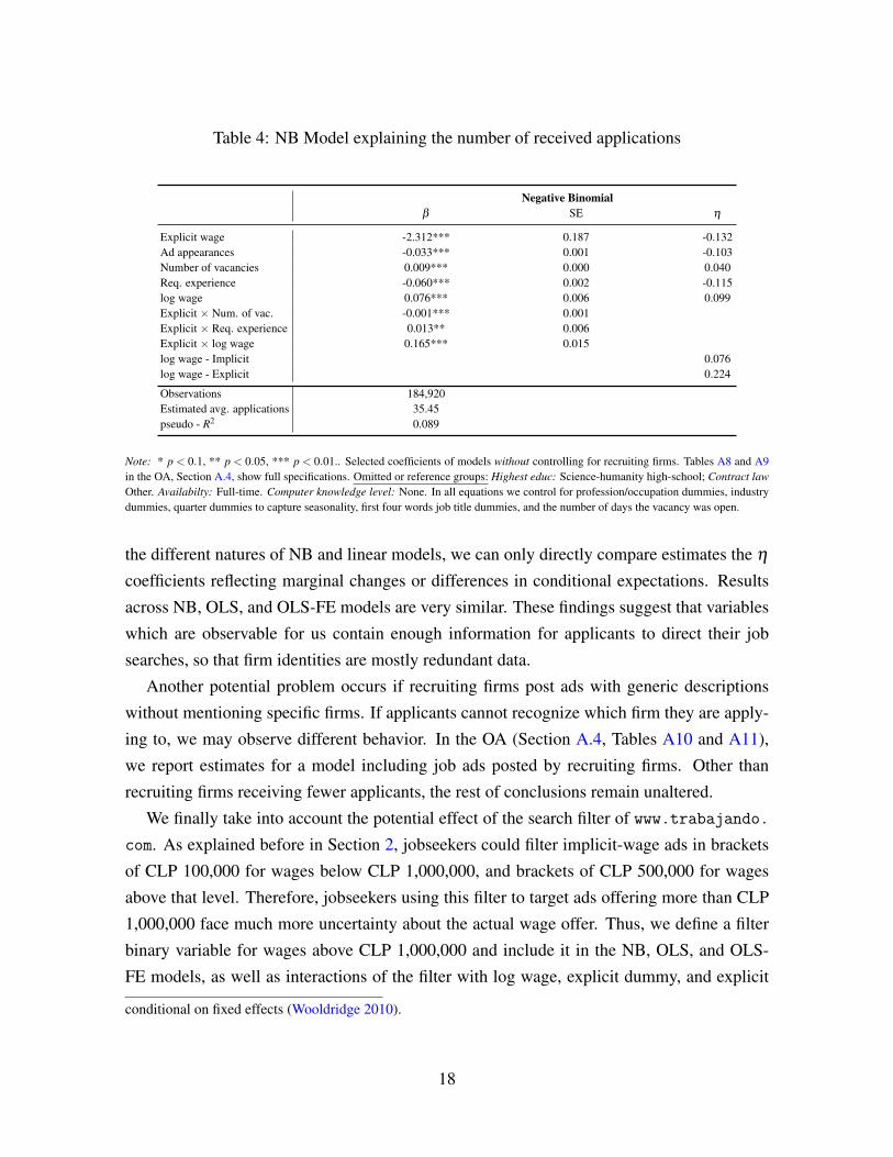
Table 4: NB Model explaining the number of received applications

Negative Binomialβ SE η

Explicit wage -2.312*** 0.187 -0.132Ad appearances -0.033*** 0.001 -0.103Number of vacancies 0.009*** 0.000 0.040Req. experience -0.060*** 0.002 -0.115log wage 0.076*** 0.006 0.099Explicit × Num. of vac. -0.001*** 0.001Explicit × Req. experience 0.013** 0.006Explicit × log wage 0.165*** 0.015log wage - Implicit 0.076log wage - Explicit 0.224

Observations 184,920Estimated avg. applications 35.45pseudo - R2 0.089

Note: * p < 0.1, ** p < 0.05, *** p < 0.01.. Selected coefficients of models without controlling for recruiting firms. Tables A8 and A9in the OA, Section A.4, show full specifications. Omitted or reference groups: Highest educ: Science-humanity high-school; Contract lawOther. Availabilty: Full-time. Computer knowledge level: None. In all equations we control for profession/occupation dummies, industrydummies, quarter dummies to capture seasonality, first four words job title dummies, and the number of days the vacancy was open.

the different natures of NB and linear models, we can only directly compare estimates the η

coefficients reflecting marginal changes or differences in conditional expectations. Results

across NB, OLS, and OLS-FE models are very similar. These findings suggest that variables

which are observable for us contain enough information for applicants to direct their job

searches, so that firm identities are mostly redundant data.

Another potential problem occurs if recruiting firms post ads with generic descriptions

without mentioning specific firms. If applicants cannot recognize which firm they are apply-

ing to, we may observe different behavior. In the OA (Section A.4, Tables A10 and A11),

we report estimates for a model including job ads posted by recruiting firms. Other than

recruiting firms receiving fewer applicants, the rest of conclusions remain unaltered.

We finally take into account the potential effect of the search filter of www.trabajando.

com. As explained before in Section 2, jobseekers could filter implicit-wage ads in brackets

of CLP 100,000 for wages below CLP 1,000,000, and brackets of CLP 500,000 for wages

above that level. Therefore, jobseekers using this filter to target ads offering more than CLP

1,000,000 face much more uncertainty about the actual wage offer. Thus, we define a filter

binary variable for wages above CLP 1,000,000 and include it in the NB, OLS, and OLS-

FE models, as well as interactions of the filter with log wage, explicit dummy, and explicit

conditional on fixed effects (Wooldridge 2010).

18

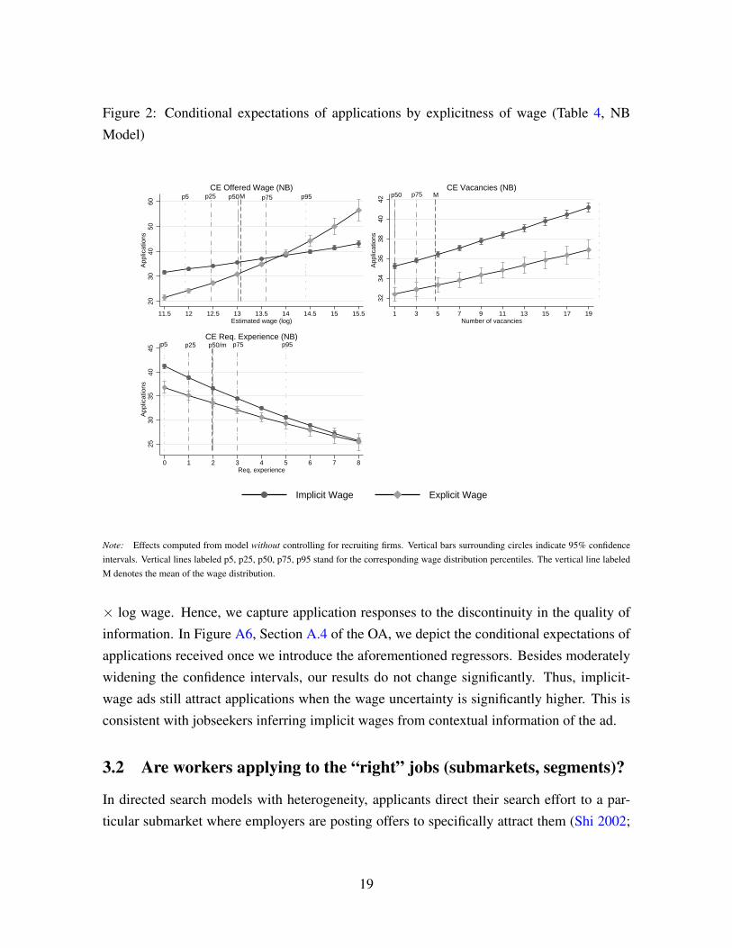
Figure 2: Conditional expectations of applications by explicitness of wage (Table 4, NB

Model)

p5 p25 p50M p75 p95

2030

4050

60A

pplic

atio

ns

11.5 12 12.5 13 13.5 14 14.5 15 15.5Estimated wage (log)

CE Offered Wage (NB)p50 p75 M

3234

3638

4042

App

licat

ions

1 3 5 7 9 11 13 15 17 19Number of vacancies

CE Vacancies (NB)

p5 p25 p50/m p75 p95

2530

3540

45A

pplic

atio

ns

0 1 2 3 4 5 6 7 8Req. experience

CE Req. Experience (NB)

Implicit Wage Explicit Wage

Note: Effects computed from model without controlling for recruiting firms. Vertical bars surrounding circles indicate 95% confidenceintervals. Vertical lines labeled p5, p25, p50, p75, p95 stand for the corresponding wage distribution percentiles. The vertical line labeledM denotes the mean of the wage distribution.

× log wage. Hence, we capture application responses to the discontinuity in the quality of

information. In Figure A6, Section A.4 of the OA, we depict the conditional expectations of

applications received once we introduce the aforementioned regressors. Besides moderately

widening the confidence intervals, our results do not change significantly. Thus, implicit-

wage ads still attract applications when the wage uncertainty is significantly higher. This is

consistent with jobseekers inferring implicit wages from contextual information of the ad.

3.2 Are workers applying to the “right” jobs (submarkets, segments)?

In directed search models with heterogeneity, applicants direct their search effort to a par-

ticular submarket where employers are posting offers to specifically attract them (Shi 2002;

19

Menzio et al. 2016). Thus, the directed search mechanism generates endogenous segmen-

tation of the labor market. We assess the relevance of this prediction in two complementary

ways.

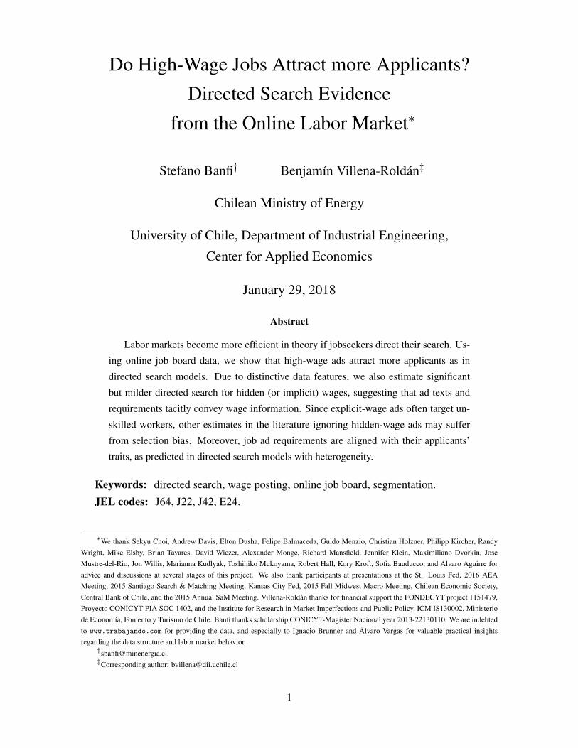
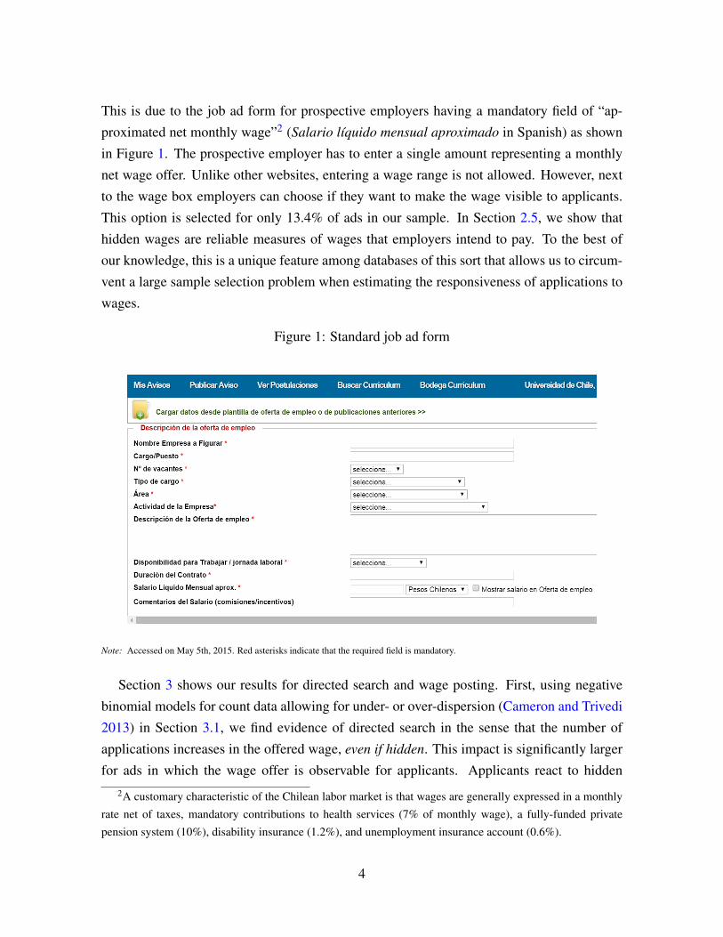
First, we ask if job ad requirements, such as experience and schooling, are correlated

with the corresponding average attributes of the received applications. In the upper-left panel

of Figure 3, we fit a linear and a Local Polynomial Regression (LPR) between the average

experience of the applicants for a given job and the corresponding ad required experience. To

assess the strength of this increasing relation, we compute a 99% confidence interval for the

LPR. The figure shows that ads with no required experience (zero) receive applicants with

an average of five years of self-declared experience. This is due to the abundance of job ads

for unexperienced workers. Moreover, since the experience requirement conveys a minimum

bar, more experienced applicants still fit the profile. For jobs requiring less than five years,

the LPR shows little variance. Beyond that point, the LPR flattens suggesting that required

and actual experience level out in that region. The increasing relation between minimum

experience required and average applicant experience is a clear indication of self-selection

into the right submarket, in line with directed search models with heterogeneous agents.

There is clear segmentation by educational level. The upper-right panel of Figure 3 fits a

LPR correlating the imputed schooling years requirement for job ads and the corresponding

average imputed schooling years of applicants. The conversion between education attained

and schooling years is explained in Section 2.1. Applicants clearly comply to ad require-

ments. Nevertheless, the LPR shows that job ads with primary education requirement (eight

years) attract applicants with average schooling of more than 12 years. For requirements of

technical tertiary education (16 years) or college graduation (17 years), the available pool of

applicants meet the specific requirement more closely. Since the overall schooling level of

the applicants is high (around 15 years) it is likely that ads with low educational requirements

receive overqualified applicants more often on average.

The two remaining panels of Figure 3 show a LPR between log offered wages (implicit

and explicit) and the average log expected wage of individuals applying for those jobs. We

observe a clear positive correlation. For implicit wages, the polynomial local regression

is slightly decreasing at exp(12.5) ≈ CLP 270,000 ≈ USD 523 per month, which shows

that workers applying for implicit low wage ads have overoptimistic expectations. In the

upper portion of the LPR, we observe a sightly decreasing portion, showing the opposite

pattern in that region. The 99% confidence interval has a similar width for different levels,

showing a constant degree of variation in average log expected wages of applicants around

20

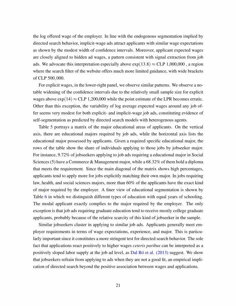
the log offered wage of the employer. In line with the endogenous segmentation implied by

directed search behavior, implicit-wage ads attract applicants with similar wage expectations

as shown by the modest width of confidence intervals. Moreover, applicant expected wages

are closely aligned to hidden ad wages, a pattern consistent with signal extraction from job

ads. We advocate this interpretation especially above exp(13.8)≈ CLP 1,000,000 , a region

where the search filter of the website offers much more limited guidance, with wide brackets

of CLP 500,000.

For explicit wages, in the lower-right panel, we observe similar patterns. We observe a no-

table widening of the confidence intervals due to the relatively small sample size for explicit

wages above exp(14)≈ CLP 1,200,000 while the point estimate of the LPR becomes erratic.

Other than this exception, the variability of log average expected wages around any job of-

fer seems very modest for both explicit- and implicit-wage job ads, constituting evidence of

self-segmentation as predicted by directed search models with heterogenous agents.

Table 5 portrays a matrix of the major educational areas of applicants. On the vertical

axis, there are educational majors required by job ads, while the horizontal axis lists the

educational major possessed by applicants. Given a required specific educational major, the

rows of the table show the share of individuals applying to those jobs by jobseeker major.

For instance, 9.72% of jobseekers applying to job ads requiring a educational major in Social

Sciences (5) have a Commerce & Management major, while a 68.32% of them hold a diploma

that meets the requirement. Since the main diagonal of the matrix shows high percentages,

applicants tend to apply more for jobs explicitly matching their own major. In jobs requiring

law, health, and social sciences majors, more than 60% of the applicants have the exact kind

of major required by the employer. A finer view of educational segmentation is shown by

Table 6 in which we distinguish different types of education with equal years of schooling.

The modal applicant exactly complies to the major required by the employer. The only

exception is that job ads requiring graduate education tend to receive mostly college graduate

applicants, probably because of the relative scarcity of this kind of jobseeker in the sample.

Similar jobseekers cluster in applying to similar job ads. Applicants generally meet em-

ployer requirements in terms of wage expectations, experience, and major. This is particu-

larly important since it constitutes a more stringent test for directed search behavior. The sole

fact that applications react positively to higher wages ceteris paribus can be interpreted as a

positively sloped labor supply at the job ad level, as Dal Bo et al. (2013) suggest. We show

that jobseekers refrain from applying to ads when they are not a good fit, an empirical impli-

cation of directed search beyond the positive association between wages and applications.

21

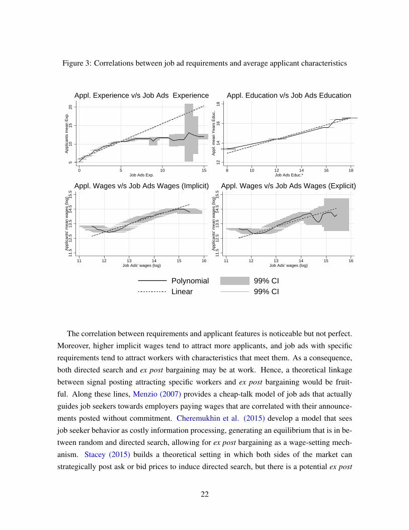
Figure 3: Correlations between job ad requirements and average applicant characteristics5

1015

20A

pplic

ants

mea

n E

xp.

0 5 10 15Job Ads Exp.

Appl. Experience v/s Job Ads Experience

1214

1618

App

l. m

ean

Yea

rs E

duc.

8 10 12 14 16 18Job Ads Educ.*

Appl. Education v/s Job Ads Education

11.5

12.5

13.5

14.5

15.5

App

lican

ts' m

ean

wag

es (

log)

11 12 13 14 15 16Job Ads' wages (log)

Appl. Wages v/s Job Ads Wages (Implicit)

11.5

12.5

13.5

14.5

15.5

App

lican

ts' m

ean

wag

es (

log)

11 12 13 14 15 16Job Ads' wages (log)

Appl. Wages v/s Job Ads Wages (Explicit)

Polynomial 99% CILinear 99% CI

The correlation between requirements and applicant features is noticeable but not perfect.

Moreover, higher implicit wages tend to attract more applicants, and job ads with specific

requirements tend to attract workers with characteristics that meet them. As a consequence,

both directed search and ex post bargaining may be at work. Hence, a theoretical linkage

between signal posting attracting specific workers and ex post bargaining would be fruit-

ful. Along these lines, Menzio (2007) provides a cheap-talk model of job ads that actually

guides job seekers towards employers paying wages that are correlated with their announce-

ments posted without commitment. Cheremukhin et al. (2015) develop a model that sees

job seeker behavior as costly information processing, generating an equilibrium that is in be-

tween random and directed search, allowing for ex post bargaining as a wage-setting mech-

anism. Stacey (2015) builds a theoretical setting in which both sides of the market can

strategically post ask or bid prices to induce directed search, but there is a potential ex post

22

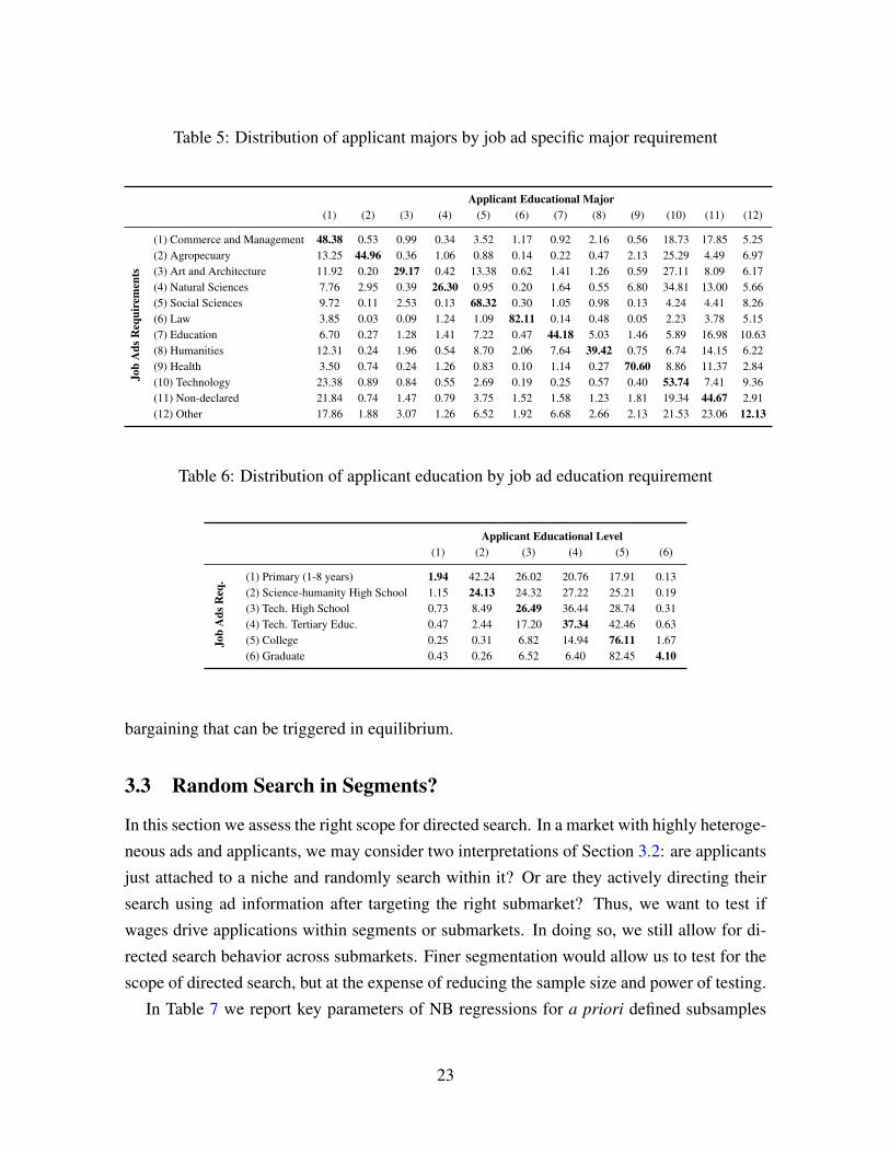
Table 5: Distribution of applicant majors by job ad specific major requirement

Applicant Educational Major(1) (2) (3) (4) (5) (6) (7) (8) (9) (10) (11) (12)

Job

Ads

Req

uire

men

ts

(1) Commerce and Management 48.38 0.53 0.99 0.34 3.52 1.17 0.92 2.16 0.56 18.73 17.85 5.25(2) Agropecuary 13.25 44.96 0.36 1.06 0.88 0.14 0.22 0.47 2.13 25.29 4.49 6.97(3) Art and Architecture 11.92 0.20 29.17 0.42 13.38 0.62 1.41 1.26 0.59 27.11 8.09 6.17(4) Natural Sciences 7.76 2.95 0.39 26.30 0.95 0.20 1.64 0.55 6.80 34.81 13.00 5.66(5) Social Sciences 9.72 0.11 2.53 0.13 68.32 0.30 1.05 0.98 0.13 4.24 4.41 8.26(6) Law 3.85 0.03 0.09 1.24 1.09 82.11 0.14 0.48 0.05 2.23 3.78 5.15(7) Education 6.70 0.27 1.28 1.41 7.22 0.47 44.18 5.03 1.46 5.89 16.98 10.63(8) Humanities 12.31 0.24 1.96 0.54 8.70 2.06 7.64 39.42 0.75 6.74 14.15 6.22(9) Health 3.50 0.74 0.24 1.26 0.83 0.10 1.14 0.27 70.60 8.86 11.37 2.84(10) Technology 23.38 0.89 0.84 0.55 2.69 0.19 0.25 0.57 0.40 53.74 7.41 9.36(11) Non-declared 21.84 0.74 1.47 0.79 3.75 1.52 1.58 1.23 1.81 19.34 44.67 2.91(12) Other 17.86 1.88 3.07 1.26 6.52 1.92 6.68 2.66 2.13 21.53 23.06 12.13

Table 6: Distribution of applicant education by job ad education requirement

Applicant Educational Level(1) (2) (3) (4) (5) (6)

Job

Ads

Req

. (1) Primary (1-8 years) 1.94 42.24 26.02 20.76 17.91 0.13(2) Science-humanity High School 1.15 24.13 24.32 27.22 25.21 0.19(3) Tech. High School 0.73 8.49 26.49 36.44 28.74 0.31(4) Tech. Tertiary Educ. 0.47 2.44 17.20 37.34 42.46 0.63(5) College 0.25 0.31 6.82 14.94 76.11 1.67(6) Graduate 0.43 0.26 6.52 6.40 82.45 4.10

bargaining that can be triggered in equilibrium.

3.3 Random Search in Segments?

In this section we assess the right scope for directed search. In a market with highly heteroge-

neous ads and applicants, we may consider two interpretations of Section 3.2: are applicants

just attached to a niche and randomly search within it? Or are they actively directing their

search using ad information after targeting the right submarket? Thus, we want to test if

wages drive applications within segments or submarkets. In doing so, we still allow for di-

rected search behavior across submarkets. Finer segmentation would allow us to test for the

scope of directed search, but at the expense of reducing the sample size and power of testing.

In Table 7 we report key parameters of NB regressions for a priori defined subsamples

23

to estimate potentially heterogeneous reactions of applicants to wages across segments. We

divide job ads in professional area requirements defined by Commerce, Technology, and

Non-Declared. Simultaneously, we also classify our sample by educational requirements

considering Scientific-Humanities High School, Technical High School, Technical Tertiary

Education, and College. These twelve segments defined by the crossover of these categories

cover 90.5% of the sample of job ads. As in Section 3.1, β is the model parameter and η the

average elasticity or differential response.

Across segments, explicit-wage ads consistently receive fewer applications than their

implicit-wage counterparts. We also find a lower but positive sensitivity of the number of

applications to wages in highly-educated segments. This mainly occurs in the Technology

and Commerce areas, and less for workers in non-declared areas. For example, while a

1% increment of offered wages raises applications 0.286% in the segment regular Science-

Humanity High School & Commerce (the log wage elasticity η in the upper-left panel), it

only increases applications by 0.075% in the segment College & Commerce (the log wage

elasticity η in the lower-left panel). Moreover, we observe a that the positive effect of explicit

wages on applications is stronger for low-education segments.

Applicant responses are heterogeneous across segments. Low-educated workers are more

sensitive to offered wages, and the high-educated ones to experience requirements. A ra-

tionale for these findings is that unskilled workers apply to simple jobs in which the most

important attribute is the wage offer, while jobseekers with high education or experience can

access higher wages by fulfilling the ad requirements.

We also approach segmentation more agnostically by relying on an unsupervised machine

learning technique, the k-means classification algorithm (Everitt et al. 2011, for instance).

With this technique, we split the sample of ads into k = 50 segments. We estimate a linear

OLS model to investigate directed search behavior for each segment. For nearly 3/4 of the

cases, we cannot reject that the estimate of sensitivity of the number of applicants to wages

is the same we obtain for the whole sample at 95% confidence. Nevertheless, 2/3 of the

95% confidence intervals for these parameters contain zero. Considering that each model

is estimated with roughly 2% of the whole sample, the evidence regarding directed search

within submarkets is naturally weaker than for the whole market. However, it is quite aligned

with the findings above for market segments defined by professional area and education. We

refer the reader to the OA, Section A.5, to see the results based on k-means segmentation in

depth.

24

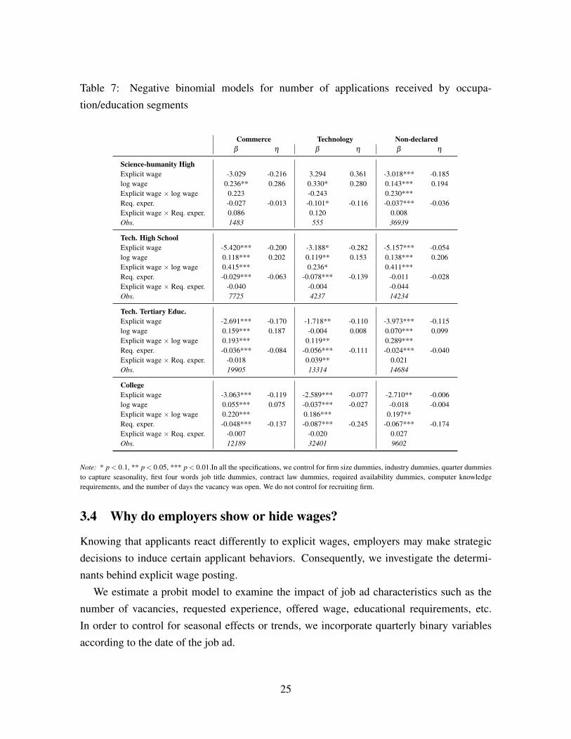
Table 7: Negative binomial models for number of applications received by occupa-

tion/education segments

Commerce Technology Non-declaredβ η β η β η

Science-humanity HighExplicit wage -3.029 -0.216 3.294 0.361 -3.018*** -0.185log wage 0.236** 0.286 0.330* 0.280 0.143*** 0.194Explicit wage × log wage 0.223 -0.243 0.230***Req. exper. -0.027 -0.013 -0.101* -0.116 -0.037*** -0.036Explicit wage × Req. exper. 0.086 0.120 0.008Obs. 1483 555 36939

Tech. High SchoolExplicit wage -5.420*** -0.200 -3.188* -0.282 -5.157*** -0.054log wage 0.118*** 0.202 0.119** 0.153 0.138*** 0.206Explicit wage × log wage 0.415*** 0.236* 0.411***Req. exper. -0.029*** -0.063 -0.078*** -0.139 -0.011 -0.028Explicit wage × Req. exper. -0.040 -0.004 -0.044Obs. 7725 4237 14234

Tech. Tertiary Educ.Explicit wage -2.691*** -0.170 -1.718** -0.110 -3.973*** -0.115log wage 0.159*** 0.187 -0.004 0.008 0.070*** 0.099Explicit wage × log wage 0.193*** 0.119** 0.289***Req. exper. -0.036*** -0.084 -0.056*** -0.111 -0.024*** -0.040Explicit wage × Req. exper. -0.018 0.039** 0.021Obs. 19905 13314 14684

CollegeExplicit wage -3.063*** -0.119 -2.589*** -0.077 -2.710** -0.006log wage 0.055*** 0.075 -0.037*** -0.027 -0.018 -0.004Explicit wage × log wage 0.220*** 0.186*** 0.197**Req. exper. -0.048*** -0.137 -0.087*** -0.245 -0.067*** -0.174Explicit wage × Req. exper. -0.007 -0.020 0.027Obs. 12189 32401 9602

Note: * p < 0.1, ** p < 0.05, *** p < 0.01.In all the specifications, we control for firm size dummies, industry dummies, quarter dummiesto capture seasonality, first four words job title dummies, contract law dummies, required availability dummies, computer knowledgerequirements, and the number of days the vacancy was open. We do not control for recruiting firm.

3.4 Why do employers show or hide wages?

Knowing that applicants react differently to explicit wages, employers may make strategic

decisions to induce certain applicant behaviors. Consequently, we investigate the determi-

nants behind explicit wage posting.

We estimate a probit model to examine the impact of job ad characteristics such as the

number of vacancies, requested experience, offered wage, educational requirements, etc.

In order to control for seasonal effects or trends, we incorporate quarterly binary variables

according to the date of the job ad.

25

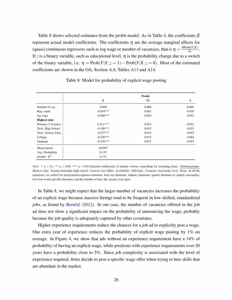
Table 8 shows selected estimates from the probit model. As in Table 4, the coefficients β

represent actual model coefficients. The coefficients η are the average marginal effects for

(quasi) continuous regressors such as log wage or number of vacancies, that is η = ∂Prob(Y |X)∂ z .

If z is a binary variable, such as educational level, η is the probability change due to a switch

of the binary variable, i.e. η = Prob(Y |X ,z = 1)−Prob(Y |X ,z = 0). Most of the estimated

coefficients are shown in the OA, Section A.6, Tables A13 and A14.

Table 8: Model for probability of explicit wage posting

Probitβ SE η

Number of vac. 0.000 0.000 0.000Req. exper. -0.034*** 0.003 -0.010log wage -0.268*** 0.010 -0.051Highest educPrimary (1-8 years) 0.211*** 0.034 0.052Tech. High School -0.108*** 0.015 -0.023Tech. Tertiary Educ. -0.257*** 0.016 -0.052College -0.328*** 0.019 -0.064Graduate -0.276*** 0.075 -0.055

Observations 183997Avg. Probability 0.135pseudo - R2 0.131

Note: * p < 0.1, ** p < 0.05, *** p < 0.01.Selected coefficients of models without controlling for recruiting firms. Omitted groups:Highest educ: Science-humanity high-school; Contract law Other. Availability: Full-time. Computer knowledge level: None. In all theequations, we control for profession/occupation dummies, firm size dummies, industry dummies, quarter dummies to capture seasonality,first four words job title dummies, and the number of days the vacancy was open.

In Table 8, we might expect that the larger number of vacancies increases the probability

of an explicit wage because massive hirings tend to be frequent in low-skilled, standardized

jobs, as found by Brencic (2012). In our case, the number of vacancies offered in the job

ad does not show a significant impact on the probability of announcing the wage, probably

because the job quality is adequately captured by other covariates.

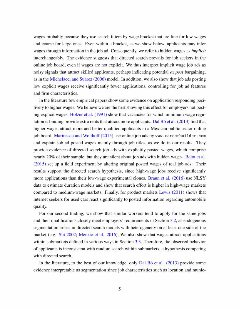
Higher experience requirements reduce the chances for a job ad to explicitly post a wage.

One extra year of experience reduces the probability of explicit wage posting by 1% on

average. In Figure 4, we show that ads without an experience requirement have a 14% of

probability of having an explicit wage, while positions with experience requirements over 20

years have a probability close to 5%. Since job complexity is associated with the level of

experience required, firms decide to post a specific wage offer when trying to hire skills that

are abundant in the market.

26

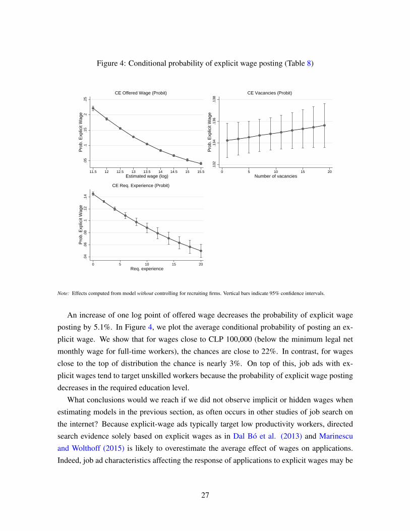
Figure 4: Conditional probability of explicit wage posting (Table 8)

.05

.1.1

5.2

.25

Pro

b. E

xplic

it W

age

11.5 12 12.5 13 13.5 14 14.5 15 15.5Estimated wage (log)

CE Offered Wage (Probit)

.132

.134

.136

.138

Pro

b. E

xplic

it W

age

0 5 10 15 20Number of vacancies

CE Vacancies (Probit)

.04

.06

.08

.1.1

2.1

4P

rob.

Exp

licit

Wag

e

0 5 10 15 20Req. experience

CE Req. Experience (Probit)

Note: Effects computed from model without controlling for recruiting firms. Vertical bars indicate 95% confidence intervals.

An increase of one log point of offered wage decreases the probability of explicit wage

posting by 5.1%. In Figure 4, we plot the average conditional probability of posting an ex-

plicit wage. We show that for wages close to CLP 100,000 (below the minimum legal net

monthly wage for full-time workers), the chances are close to 22%. In contrast, for wages

close to the top of distribution the chance is nearly 3%. On top of this, job ads with ex-

plicit wages tend to target unskilled workers because the probability of explicit wage posting

decreases in the required education level.

What conclusions would we reach if we did not observe implicit or hidden wages when

estimating models in the previous section, as often occurs in other studies of job search on

the internet? Because explicit-wage ads typically target low productivity workers, directed

search evidence solely based on explicit wages as in Dal Bo et al. (2013) and Marinescu

and Wolthoff (2015) is likely to overestimate the average effect of wages on applications.

Indeed, job ad characteristics affecting the response of applications to explicit wages may be

27

simultaneously determining the probability of explicit wage posting. Therefore, inferring the

true effect of wages on applications is subject to a sample selection problem.

A wage increase not only affects the number of applicants received, but also the proba-

bility that the employer makes the wage offer explicit. In the OA, Section A.7, we derive a

theoretical condition to obtain an unbiased estimate for application-wage sensitivity solely

based on explicit wages ads. Such condition, involving application-wage elasticities and

other estimated magnitudes, does not empirically hold. Thus, we conclude that the estimated

application-wage sensitivity for only explicit wages overestimates the average value for all

ads.

Our facts are consistent with the Michelacci and Suarez (2006) model. Under certain pa-

rameterizations, their model allows for a separating equilibrium in which high-productivity

workers apply for good jobs with hidden wages and low-productivity workers go for bad

jobs with explicit wages. Intuitively, for high-quality jobs hiding wages is a strategic choice

by employers to signal ex post bargaining when match-specific requirements are important.

Hence, if job quality is imperfectly observed, an employer choosing an implicit wage may

reveal some information, or attract applicants with specific knowledge of the job or the eco-

nomic sector. The targeted group could guess wages and other job characteristics more accu-

rately. In contrast, an explicit wage could reveal that a job does not require a match specific

skill or information, so that the job quality is perceived as low.

Our results are robust. In the OA, Section A.6, Tables A13 and A14, besides probit es-

timates, we report OLS linear probability and firm fixed effects (OLS-FE) to account for

all firm idiosyncratic unobserved factors affecting the wage explicitness decision, such as

corporate culture, or specific managerial standards. If explicit-wage posting is a corporate

policy, controlling for unobserved heterogeneity is important. While the effect of wage level

on wage-explicitness decreases noticeably if we control for firm-fixed effects, it remains neg-

ative and significant. Hence, job characteristics affect explicit wage-posting even within the

same firm.

We also show that these linear models controlling for recruiting firms since they may be

hired to post ads for a particular type of jobs. In the OA, Section A.6, Tables A15 and A16

we show that the average marginal effects barely change with respect to the baseline.

28

4 Conclusions

Our evidence shows that directed search is a prevalent behavior in the online labor market

studied. Thanks to the remarkable availability of offered wages for a sizable share of ads in

the job board studied, we can circumvent the large selection bias arising in other databases,

which typically cannot analyze more than 25% of their job ads.

Applicants react to information provided by employers such as offered wages or educa-

tional requirements, as predicted by standard directed search models. We show that workers

apply more for jobs offering higher wages even if employers choose to hide them, after con-

trolling for a detailed set of job characteristics, including requirements over education level,

major, experience, job title binary variables, and even firm fixed effects. Nevertheless, appli-

cants are more sensitive to changes in wages when they are explicit and less when they are

hidden. Explicit-wage job ads provide a low-noise signal to applicants, driving their search

behavior more decisively. In turn, the evidence suggests that applicants infer hidden wages

from job ads, so we refer to them as implicit wages.

A second more stringent testable prediction of directed search behavior is that workers

apply for job ads targeting them in a specific submarket. We slice the data in several ways to

show that there is a notable alignment between job ad requirements and worker characteris-

tics in terms of offered/expected wage, educational level, occupation, and experience. These

results notably hold for implicit wages as well.

Evidence suggests that employers use explicit/implicit wage posting strategies to reduce

the pool of applicants and increase their quality or suitability. Low marginal application costs

potentially spurs too many applications, imposing a large screening burden on the employers’

side. By making explicit wage offers for simple jobs, employers dissuade too many applica-

tions when differentiation among candidates is rarely a concern and take-it-or-leave-it offers

prevail. On the other side of the wage distribution, differentiation across candidates matters

and employers often prefer implicit wages, perhaps as a way to signal they are open for bar-

gaining, in line with the theory of Michelacci and Suarez (2006). Consistent with this view,

we also show that employers tend to post explicit wages in job ads with low educational and

experience requirements.

Beyond labor market efficiency implications, a practical lesson is that there is a large

scope for strategic communication and job ad design for firms in order to attract the kind and

number of applicants they desire. This is important since hiring involves a costly selection

process among heterogeneously productive workers, especially for job positions for skilled

workers (Oyer and Schaefer 2011; Muehlemann and Pfeifer 2016).

29

References

Abowd, J. M., F. Kramarz, and D. N. Margolis (1999). High Wage Workers and High

Wage Firms. Econometrica 2(67), 251–333.

Acemoglu, D. (1997). Training and Innovation in an Imperfect Labour Market. The Re-

view of Economic Studies 64(3), 445–464.

Acemoglu, D. (2001). Good Jobs versus Bad Jobs. Journal of Labor Economics 19(1),

1–21.

Acemoglu, D. and R. Shimer (2000). Productivity Gains from Unemployment Insurance.

European Economic Review 44(7), 1195–1224.

Albrecht, J., P. A. Gautier, and S. Vroman (2006). Equilibrium Directed Search with Mul-

tiple Applications. Review of Economic Studies 73(4), 869–891.

Autor, D. H. (2001). Wiring the Labor Market. Journal of Economic Perspectives 15(1),

25–40.

Banfi, S., S. Choi, and B. Villena-Roldan (2017). Deconstructing job search. Mimeo.

Barron, J. M., J. Bishop, and W. C. Dunkelberg (1985). Employer search: The inter-

viewing and hiring of new employees. The Review of Economics and Statistics 67(1),

43–52.

Belot, M., P. Kircher, and P. Muller (2015, May). How Wage Annoucements Affect

Job Search Behaviour: a Field Experimental Investigation. 2015 Annual Search and

Matching Group Meeting. Aix-en-Provence, France.

Braun, C., B. Engelhardt, B. Griffy, and P. Rupert (2016). Do workers direct their search?

Technical report. Mimeo.

Brencic, V. (2012). Wage Posting: Evidence from Job Ads. Canadian Journal of Eco-

nomics/Revue canadienne d’economique 45(4), 1529–1559.

Brenzel, H., H. Gartner, and C. Schnabel (2014). Wage bargaining or wage posting? Evi-

dence from the employers’ side. Labour Economics 29(0), 41 – 48.

Calinski, T. and J. Harabasz (1974). A Dendrite Method for Cluster Analysis. Communi-

cations in Statistics- Theory and Methods 3(1), 1–27.

Cameron, A. C. and P. K. Trivedi (2013). Regression Analysis of Count Data, Volume 53.

Cambridge University Press.

30

Chandler, D., J. Horton, and R. Johari (2015). Market Congestion and Application Costs.

Technical report. Society of Labor Economics Annual Meeting.

Cheremukhin, A., P. Restrepo-Echavarria, and A. Tutino (2015). A Theory of Targeted

Search. Working Paper 2014-035B, Federal Reserve Bank of St. Louis.

Dal Bo, E., F. Finan, and M. A. Rossi (2013). Strengthening state capabilities: The role

of financial incentives in the call to public service. The Quarterly Journal of Eco-

nomics 128(3), 1169–1218.

Ellingsen, T. and A. Rosen (2003). Fixed or Flexible? Wage-setting in Search Equilibrium.

Economica 70(278), 233–250.

Everitt, B., S. Landau, M. Leese, and D. Stahl (2011). Cluster Analysis (5th ed.). Wiley.

Flinn, C. J. (2006). Minimum Wage Effects on Labor Market Outcomes under Search,

Matching, and Endogenous Contact Rates. Econometrica 74(4), 1013–1062.

Galenianos, M. and P. Kircher (2009). Directed Search with Multiple Job Applications.

Journal of Economic Theory 144(2), 445–471.

Hall, R. E. and A. B. Krueger (2012, May). Evidence on the Incidence of Wage Posting,

Wage Bargaining, and On-the-Job Search. American Economic Journal: Macroeco-

nomics 4(4), 56–67.

Holzer, H. J., L. F. Katz, and A. B. Krueger (1991). Job Queues and Wages. The Quarterly

Journal of Economics 106(3), 739–768.

Hosios, A. J. (1990). On the Efficiency of Matching and Related Models of Search and

Unemployment. The Review of Economic Studies 57(2), 279–298.

Kircher, P. (2009). Efficiency of simultaneous search. The Journal of Political Econ-

omy 117(5), pp. 861–913.

Kuhn, P. and K. Shen (2013). Gender Discrimination in Job Ads: Evidence from China.

The Quarterly Journal of Economics 128(1), 287–336.

Lewis, G. (2011). Asymmetric Information, Adverse Selection and Online Disclosure:

The Case of eBay Motors. The American Economic Review 101(4), 1535–1546.

Marinescu, I. E. and R. P. Wolthoff (2015). Opening the Black Box of the Matching Func-

tion: The Power of Words. Discussion Paper 9071, IZA.

Menzio, G. (2007). A Theory of Partially Directed Search. Journal of Political Econ-

omy 115(5), 748–769.

31

Menzio, G. and S. Shi (2010). Block recursive equilibria for stochastic models of search

on the job. Journal of Economic Theory 145(4), 1453 – 1494.

Menzio, G., I. A. Telyukova, and L. Visschers (2016). Directed search over the life cycle.

Review of Economic Dynamics 19, 38 – 62. Special Issue in Honor of Dale Mortensen.

Michelacci, C. and J. Suarez (2006). Incomplete Wage Posting. Journal of Political Econ-

omy 114(6), 1098–1123.

Moen, E. (1999). Education, Ranking, and Competition for Jobs. Journal of Labor Eco-

nomics 17(4), 694–723.

Moen, E. R. (1997). Competitive Search Equilibrium. The Journal of Political Econ-

omy 105(2), 385–411.

Moen, E. R. and A. Rosen (2004). Does Poaching Distort Training? The Review of Eco-

nomic Studies 71(4), 1143–1162.

Muehlemann, S. and H. Pfeifer (2016). The Structure of Hiring Costs in Germany: Evi-

dence from Firm-Level Data. Industrial Relations: A Journal of Economy and Soci-

ety 55(2), 193–218.

Niederle, M. and A. E. Roth (2009). The Effects of a Centralized Clearinghouse on Job

Placement, Wages, and Hiring Practices. In Studies of Labor Market Intermediation,

pp. 235–271. University of Chicago Press.

Oyer, P. and S. Schaefer (2011). Personnel Economics: Hiring and Incentives. Handbook

of Labor Economics 4, 1769–1823.

Roth, A. E. and M. Sotomayor (1992). Two-Sided Matching, Volume 1 of Handbook of

Game Theory with Economic Applications, Chapter 14, pp. 927–1007. Elsevier.

Seabright, P. and A. Sen (2014). Statistical Externalities and the Labour Market in the

Digital Age. Technical report, IDEI Working Paper.

Servicio de Informacion de Educacion Superior (2017, August). Informe de Duracion

Real y Sobreduracion de Carreras o Programas, Generacion Titulados y Graduados

2012 - 2016. Report, Chilean Ministry of Education. https://goo.gl/zGebvt . Accesed

on Aug 30th 2017.

Shi, S. (2002). A directed search model of inequality with heterogeneous skills and skill-

biased technology. The Review of Economic Studies 69(2), 467–491.

Stacey, D. (2015). Posted Prices, Search and Bargaining. Ryerson University, mimeo.

32

van Ommeren, J. and G. Russo (2014). Firm recruitment behaviour: Sequential or non-

sequential search? Oxford Bulletin of Economics and Statistics 76(3), 432–455.

van Ours, J. and G. Ridder (1992). Vacancies and the Recruitment of New Employees.

Journal of Labor Economics 10(2), 138–155.

Villena-Roldan, B. (2012). Aggregate Implications of Employer Search and Recruiting

Selection. Working Paper 271, Center for Applied Economics, University of Chile.

Wooldridge, J. M. (2010). Econometric Analysis of Cross Section and Panel Data (Second

ed.). The MIT Press.

Wright, R., P. Kircher, B. Julıen, and V. Guerrieri (2017). Directed search: A guided tour.

Technical report, National Bureau of Economic Research.

33

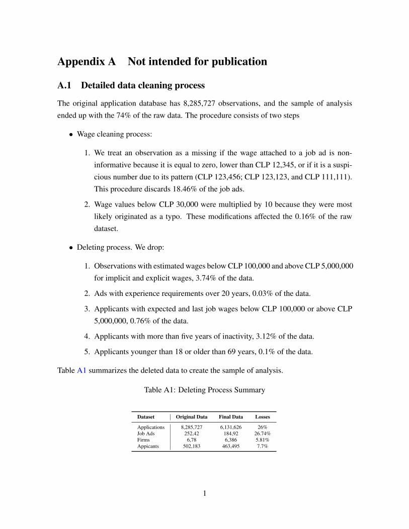
Appendix A Not intended for publication

A.1 Detailed data cleaning process

The original application database has 8,285,727 observations, and the sample of analysis

ended up with the 74% of the raw data. The procedure consists of two steps

• Wage cleaning process:

1. We treat an observation as a missing if the wage attached to a job ad is non-

informative because it is equal to zero, lower than CLP 12,345, or if it is a suspi-

cious number due to its pattern (CLP 123,456; CLP 123,123, and CLP 111,111).

This procedure discards 18.46% of the job ads.

2. Wage values below CLP 30,000 were multiplied by 10 because they were most

likely originated as a typo. These modifications affected the 0.16% of the raw

dataset.

• Deleting process. We drop:

1. Observations with estimated wages below CLP 100,000 and above CLP 5,000,000

for implicit and explicit wages, 3.74% of the data.

2. Ads with experience requirements over 20 years, 0.03% of the data.

3. Applicants with expected and last job wages below CLP 100,000 or above CLP

5,000,000, 0.76% of the data.

4. Applicants with more than five years of inactivity, 3.12% of the data.

5. Applicants younger than 18 or older than 69 years, 0.1% of the data.

Table A1 summarizes the deleted data to create the sample of analysis.

Table A1: Deleting Process Summary

Dataset Original Data Final Data Losses

Applications 8,285,727 6,131,626 26%Job Ads 252,42 184,92 26.74%Firms 6,78 6,386 5.81%Appicants 502,183 463,495 7.7%

1

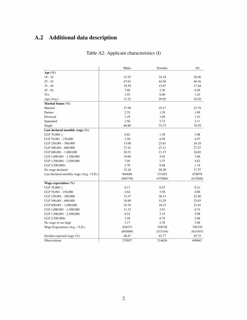
A.2 Additional data description

Table A2: Applicant characteristics (I)

Males Females AllAge (%)18 - 24 23.25 34.18 28.4625 - 34 47.61 44.56 46.1635 - 44 19.59 15.07 17.4445 - 54 7.60 5.30 6.5055+ 1.95 0.90 1.45Age (Avg.) 31.25 29.05 30.20Marital Status (%)Married 27.99 19.17 23.79Partner 2.35 1.39 1.89Divorced 1.19 1.69 1.43Separated 1.56 2.73 2.11Single 66.80 74.75 70.59Last declared monthly wage (%)CLP 70,000 ≤ 0.82 1.38 1.08CLP 70,001 - 150,000 3.58 6.50 4.97CLP 150,001 - 300,000 13.08 23.61 18.10CLP 300,001 - 600,000 27.41 27.11 27.27CLP 600,001 - 1,000,000 20.21 13.15 16.85CLP 1,000,001 - 1,500,000 10.06 5.03 7.66CLP 1,500,001 - 2,500,000 7.05 2.37 4.82CLP 2,500,000+ 2.70 0.68 1.74No wage declared 15.18 20.20 17.57Last declared monthly wage (Avg. / S.D.) 804686 531855 678878

(684730) (475868) (612840)Wage expectation (%)CLP 70,000 ≤ 0.17 0.25 0.21CLP 70,001 - 150,000 2.64 5.50 4.00CLP 150,001 - 300,000 15.37 30.13 22.40CLP 300,001 - 600,000 30.89 33.29 32.03CLP 600,001 - 1,000,000 24.76 18.23 21.65CLP 1,000,001 - 1,500,000 11.32 5.91 8.74CLP 1,500,001 - 2,500,000 8.52 3.15 5.98CLP 2,500,000+ 3.26 0.79 2.08No wage or too high 3.17 2.78 2.98Wage Expectation (Avg. / S.D.) 838753 559238 705339

(693009) (473144) (614307)Declare expected wage (%) 48.47 42.77 45.75Observations 235037 214626 449663

2

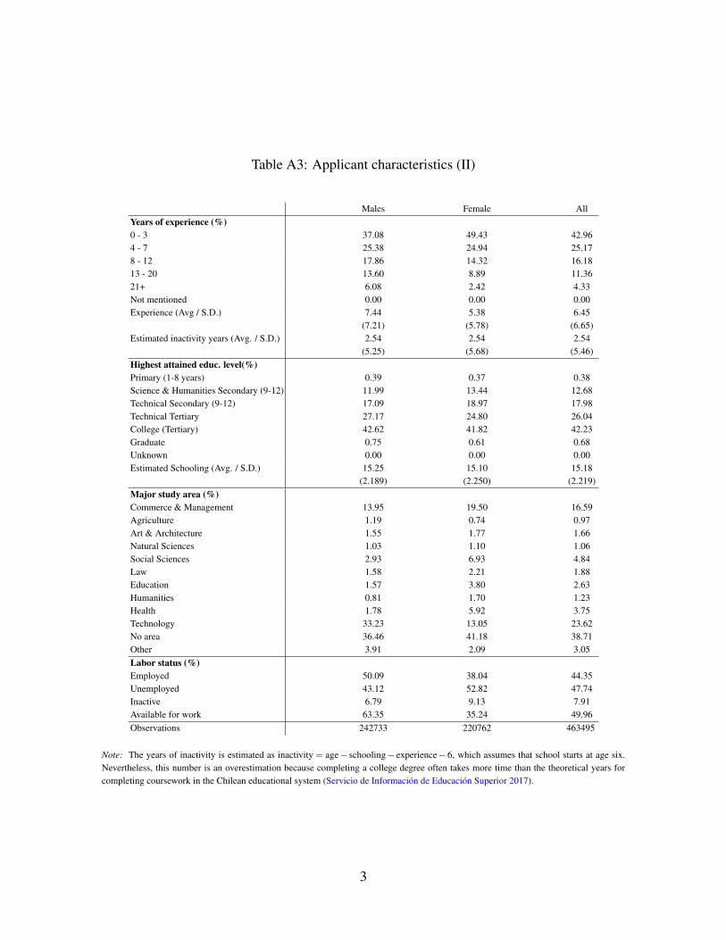
Table A3: Applicant characteristics (II)

Males Female AllYears of experience (%)0 - 3 37.08 49.43 42.964 - 7 25.38 24.94 25.178 - 12 17.86 14.32 16.1813 - 20 13.60 8.89 11.3621+ 6.08 2.42 4.33Not mentioned 0.00 0.00 0.00Experience (Avg / S.D.) 7.44 5.38 6.45

(7.21) (5.78) (6.65)Estimated inactivity years (Avg. / S.D.) 2.54 2.54 2.54

(5.25) (5.68) (5.46)Highest attained educ. level(%)Primary (1-8 years) 0.39 0.37 0.38Science & Humanities Secondary (9-12) 11.99 13.44 12.68Technical Secondary (9-12) 17.09 18.97 17.98Technical Tertiary 27.17 24.80 26.04College (Tertiary) 42.62 41.82 42.23Graduate 0.75 0.61 0.68Unknown 0.00 0.00 0.00Estimated Schooling (Avg. / S.D.) 15.25 15.10 15.18

(2.189) (2.250) (2.219)Major study area (%)Commerce & Management 13.95 19.50 16.59Agriculture 1.19 0.74 0.97Art & Architecture 1.55 1.77 1.66Natural Sciences 1.03 1.10 1.06Social Sciences 2.93 6.93 4.84Law 1.58 2.21 1.88Education 1.57 3.80 2.63Humanities 0.81 1.70 1.23Health 1.78 5.92 3.75Technology 33.23 13.05 23.62No area 36.46 41.18 38.71Other 3.91 2.09 3.05Labor status (%)Employed 50.09 38.04 44.35Unemployed 43.12 52.82 47.74Inactive 6.79 9.13 7.91Available for work 63.35 35.24 49.96Observations 242733 220762 463495

Note: The years of inactivity is estimated as inactivity = age− schooling− experience− 6, which assumes that school starts at age six.Nevertheless, this number is an overestimation because completing a college degree often takes more time than the theoretical years forcompleting coursework in the Chilean educational system (Servicio de Informacion de Educacion Superior 2017).

3

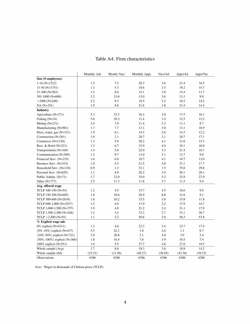
Table A4: Firm characteristics

Monthly Ads Montly Vacs Monthly Apps Vacs/Ad Apps/Ad Apps/VacSize (# employees)1-10 (N=1522) 1.5 7.5 20.3 3.6 21.4 16.511-50 (N=1751) 1.3 5.3 18.6 3.3 19.2 14.751-300 (N=583) 1.5 8.6 15.1 3.8 15.4 11.7301-1000 (N=600) 3.2 15.6 13.0 3.6 13.1 9.9>1000 (N=248) 2.2 9.3 18.5 3.2 18.2 14.2NA (N=191) 1.9 8.6 21.6 3.8 21.4 14.4IndustryAgriculture (N=271) 5.3 32.5 16.2 2.0 17.5 16.1Fishing (N=34) 5.8 29.3 11.4 1.9 12.5 12.2Mining (N=231) 2.4 7.0 11.4 2.3 11.1 8.7Manufacturing (N=981) 1.7 7.7 13.1 3.0 13.1 10.9Elect, water, gas (N=151) 1.9 6.1 14.5 2.6 14.3 12.2Construction (N=261) 1.0 2.1 20.7 2.1 20.7 17.1Commerce (N=1120) 1.3 5.9 20.2 4.1 21.0 15.2Rest. & Hotel (N=221) 1.3 6.7 33.9 4.4 34.1 16.0Transportation (N=164) 1.4 5.0 22.0 3.3 21.4 16.1Communication (N=589) 1.2 9.7 13.0 5.1 13.7 9.0Financial Serv. (N=219) 1.6 6.0 18.7 4.1 19.7 13.0Business Serv. (N=533) 1.0 4.3 21.5 4.0 23.1 17.7Household Serv. (N=134) 0.9 1.3 32.1 1.5 35.0 29.8Personal Serv. (N=629) 1.1 4.0 26.2 3.4 26.1 20.1Public Admin. (N=71) 1.7 12.0 35.0 5.3 32.9 27.9Other (N=777) 2.5 11.3 11.8 3.7 11.5 9.4Avg. offered wageTCLP 100-150 (N=54) 1.2 4.5 15.7 4.5 16.6 9.9TCLP 150-300 (N=685) 1.8 16.6 20.9 8.8 21.6 9.1TCLP 300-600 (N=2630) 1.8 10.2 15.5 3.6 15.8 11.8TCLP 600-1,000 (N=1937) 1.5 4.0 17.0 2.2 17.9 14.7TCLP 1,000-1,500 (N=757) 1.9 4.8 21.2 2.4 21.1 17.9TCLP 1,500-2,500 (N=268) 1.2 3.4 33.2 2.7 33.1 28.7TCLP >2,500 (N=55) 1.1 2.2 58.8 2.0 56.5 53.8% Explicit wage ads0% explicit (N=4311) 1.2 4.0 22.3 3.4 22.7 17.4(0%,10%] explicit (N=437) 5.5 22.1 1.8 2.6 1.1 0.7(10%,50%] explicit (N=721) 3.0 20.8 3.1 4.0 3.9 2.4(50%,100%) explicit (N=366) 1.8 16.4 7.8 3.9 10.5 7.4100% explicit (N=551) 1.0 5.5 27.7 4.8 27.0 19.5Whole sample (Avg) 1.7 8.0 18.3 3.6 18.8 14.2Whole sample (Sd) (23.31) (11.56) (40.27) (26.85) (43.36) (39.15)Observations 6386 6386 6386 6386 6386 6386

Note: Wages in thousands of Chilean pesos (TCLP).

4

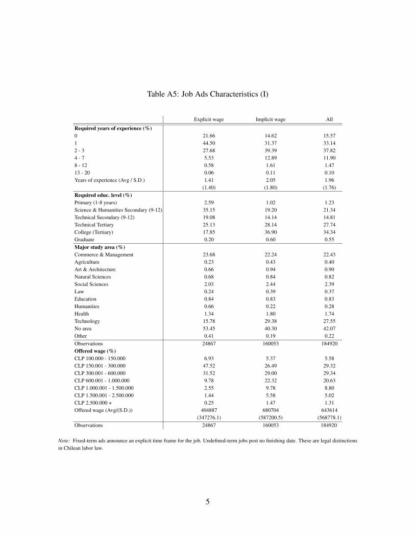
Table A5: Job Ads Characteristics (I)

Explicit wage Implicit wage All

Required years of experience (%)0 21.66 14.62 15.571 44.50 31.37 33.142 - 3 27.68 39.39 37.824 - 7 5.53 12.89 11.908 - 12 0.58 1.61 1.4713 - 20 0.06 0.11 0.10Years of experience (Avg / S.D.) 1.41 2.05 1.96

(1.40) (1.80) (1.76)Required educ. level (%)Primary (1-8 years) 2.59 1.02 1.23Science & Humanities Secondary (9-12) 35.15 19.20 21.34Technical Secondary (9-12) 19.08 14.14 14.81Technical Tertiary 25.13 28.14 27.74College (Tertiary) 17.85 36.90 34.34Graduate 0.20 0.60 0.55Major study area (%)Commerce & Management 23.68 22.24 22.43Agriculture 0.23 0.43 0.40Art & Architecture 0.66 0.94 0.90Natural Sciences 0.68 0.84 0.82Social Sciences 2.03 2.44 2.39Law 0.24 0.39 0.37Education 0.84 0.83 0.83Humanities 0.66 0.22 0.28Health 1.34 1.80 1.74Technology 15.78 29.38 27.55No area 53.45 40.30 42.07Other 0.41 0.19 0.22Observations 24867 160053 184920Offered wage (%)CLP 100.000 - 150.000 6.93 5.37 5.58CLP 150.001 - 300.000 47.52 26.49 29.32CLP 300.001 - 600.000 31.52 29.00 29.34CLP 600.001 - 1.000.000 9.78 22.32 20.63CLP 1.000.001 - 1.500.000 2.55 9.78 8.80CLP 1.500.001 - 2.500.000 1.44 5.58 5.02CLP 2.500.000 + 0.25 1.47 1.31Offered wage (Avg/(S.D.)) 404887 680704 643614

(347276.1) (587200.5) (568778.1)Observations 24867 160053 184920

Note: Fixed-term ads announce an explicit time frame for the job. Undefined-term jobs post no finishing date. These are legal distinctionsin Chilean labor law.

5

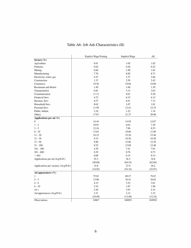
Table A6: Job Ads Characteristics (II)

Explicit Wage Posting Implicit Wage AllSectors (%)Agriculture 0.81 1.05 1.02Fisheries 0.02 0.26 0.22Mining 0.68 1.98 1.81Manufacturing 7.76 8.85 8.71Electricity, water, gas 4.47 2.37 2.66Construction 1.37 2.59 2.42Commerce 19.56 19.84 19.80Restaurant and Hotels 1.49 1.60 1.59Transportation 6.81 3.13 3.63Communication 11.12 9.01 9.30Financial Serv. 4.72 6.33 6.12Business Serv. 8.57 6.91 7.13Household Serv. 0.62 1.07 1.01Personal Serv. 11.99 12.41 12.35Public Admin. 2.16 1.22 1.34Others 17.87 21.37 20.90Applications per ad (%)0 14.44 14.94 14.871 - 2 10.91 6.62 7.203 - 5 12.16 7.96 8.536 - 10 13.83 10.66 11.0911 - 20 16.23 15.36 15.4821 - 30 9.15 10.36 10.2031 - 50 9.88 12.66 12.2951 - 100 8.52 13.09 12.48101 - 300 4.39 7.41 7.01301 - 600 0.39 0.78 0.73> 601 0.08 0.15 0.14Applications per ad (Avg/S.D.) 25.3 36.3 34.8

(49.68) (64.52) (62.84)Applications per vacancy (Avg/S.D.) 15.8 27.9 26.2

(34.05) (54.16) (52.07)Ad appearances (%)1 75.83 80.27 79.672 - 3 12.00 10.41 10.624 - 6 4.15 3.52 3.616 - 10 2.54 1.87 1.9610 + 5.49 3.93 4.14Ad appearances (Avg/S.D.) 3.31 3.12 3.15

(10.49) (12.48) (12.24)Observations 24867 160053 184920

6

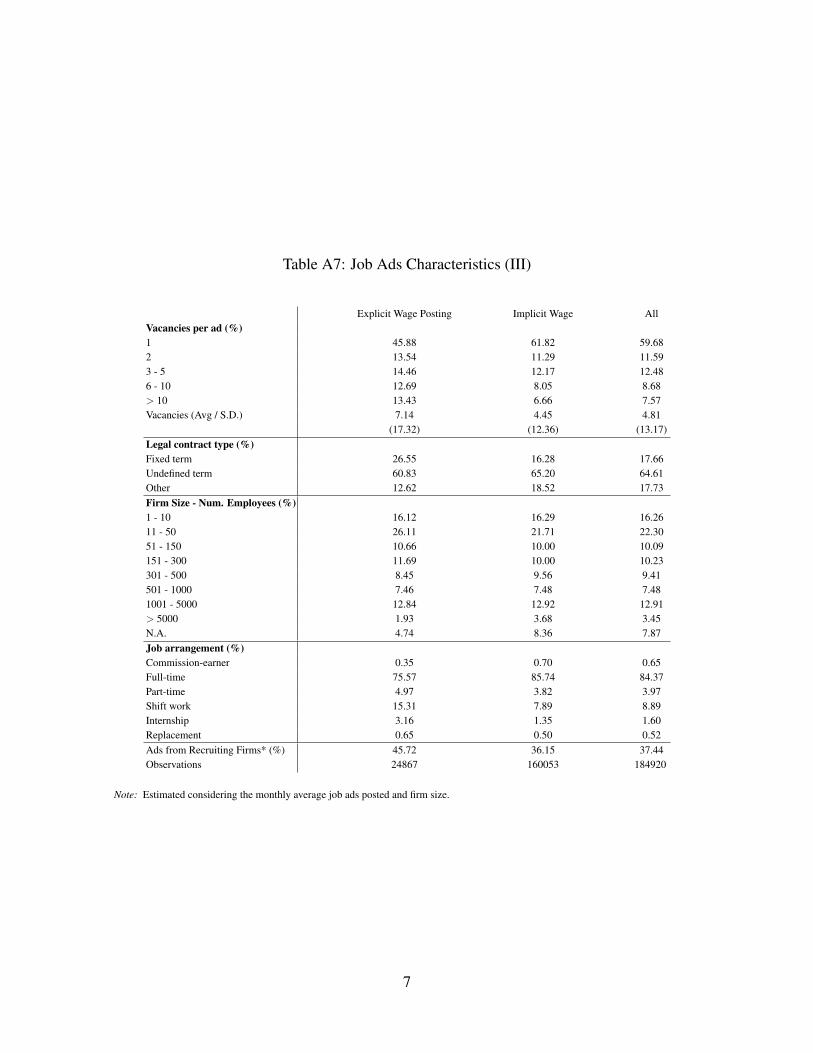
Table A7: Job Ads Characteristics (III)

Explicit Wage Posting Implicit Wage AllVacancies per ad (%)1 45.88 61.82 59.682 13.54 11.29 11.593 - 5 14.46 12.17 12.486 - 10 12.69 8.05 8.68> 10 13.43 6.66 7.57Vacancies (Avg / S.D.) 7.14 4.45 4.81

(17.32) (12.36) (13.17)Legal contract type (%)Fixed term 26.55 16.28 17.66Undefined term 60.83 65.20 64.61Other 12.62 18.52 17.73Firm Size - Num. Employees (%)1 - 10 16.12 16.29 16.2611 - 50 26.11 21.71 22.3051 - 150 10.66 10.00 10.09151 - 300 11.69 10.00 10.23301 - 500 8.45 9.56 9.41501 - 1000 7.46 7.48 7.481001 - 5000 12.84 12.92 12.91> 5000 1.93 3.68 3.45N.A. 4.74 8.36 7.87Job arrangement (%)Commission-earner 0.35 0.70 0.65Full-time 75.57 85.74 84.37Part-time 4.97 3.82 3.97Shift work 15.31 7.89 8.89Internship 3.16 1.35 1.60Replacement 0.65 0.50 0.52Ads from Recruiting Firms* (%) 45.72 36.15 37.44Observations 24867 160053 184920

Note: Estimated considering the monthly average job ads posted and firm size.

7

A.3 Word cloud for job titles

Figure A1: Job Ad Titles with Implicit Wages

Note: Generated in www.tagul.com

8

Figure A2: Job Ad Titles with Explicit Wages

Note: Generated in www.tagul.com

9

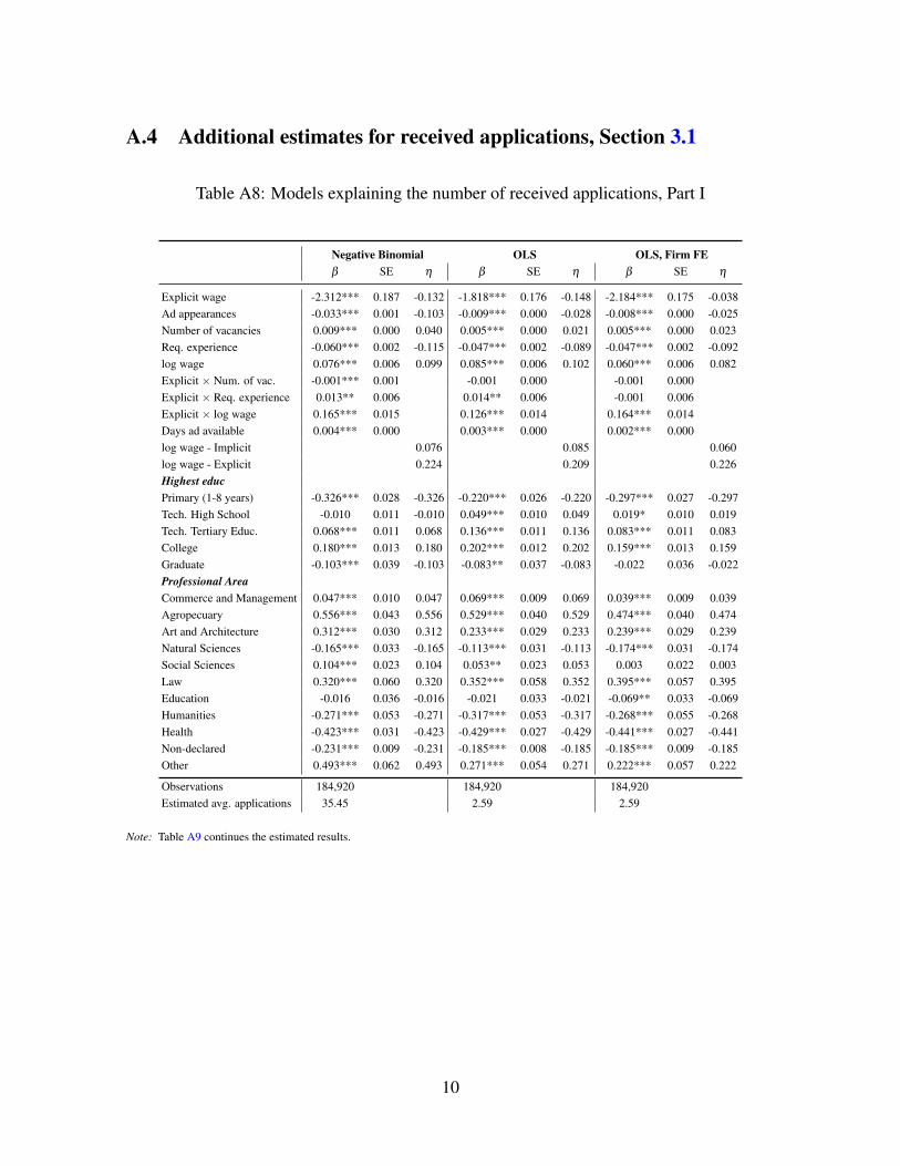
A.4 Additional estimates for received applications, Section 3.1

Table A8: Models explaining the number of received applications, Part I

Negative Binomial OLS OLS, Firm FEβ SE η β SE η β SE η

Explicit wage -2.312*** 0.187 -0.132 -1.818*** 0.176 -0.148 -2.184*** 0.175 -0.038Ad appearances -0.033*** 0.001 -0.103 -0.009*** 0.000 -0.028 -0.008*** 0.000 -0.025Number of vacancies 0.009*** 0.000 0.040 0.005*** 0.000 0.021 0.005*** 0.000 0.023Req. experience -0.060*** 0.002 -0.115 -0.047*** 0.002 -0.089 -0.047*** 0.002 -0.092log wage 0.076*** 0.006 0.099 0.085*** 0.006 0.102 0.060*** 0.006 0.082Explicit × Num. of vac. -0.001*** 0.001 -0.001 0.000 -0.001 0.000Explicit × Req. experience 0.013** 0.006 0.014** 0.006 -0.001 0.006Explicit × log wage 0.165*** 0.015 0.126*** 0.014 0.164*** 0.014Days ad available 0.004*** 0.000 0.003*** 0.000 0.002*** 0.000log wage - Implicit 0.076 0.085 0.060log wage - Explicit 0.224 0.209 0.226Highest educPrimary (1-8 years) -0.326*** 0.028 -0.326 -0.220*** 0.026 -0.220 -0.297*** 0.027 -0.297Tech. High School -0.010 0.011 -0.010 0.049*** 0.010 0.049 0.019* 0.010 0.019Tech. Tertiary Educ. 0.068*** 0.011 0.068 0.136*** 0.011 0.136 0.083*** 0.011 0.083College 0.180*** 0.013 0.180 0.202*** 0.012 0.202 0.159*** 0.013 0.159Graduate -0.103*** 0.039 -0.103 -0.083** 0.037 -0.083 -0.022 0.036 -0.022Professional AreaCommerce and Management 0.047*** 0.010 0.047 0.069*** 0.009 0.069 0.039*** 0.009 0.039Agropecuary 0.556*** 0.043 0.556 0.529*** 0.040 0.529 0.474*** 0.040 0.474Art and Architecture 0.312*** 0.030 0.312 0.233*** 0.029 0.233 0.239*** 0.029 0.239Natural Sciences -0.165*** 0.033 -0.165 -0.113*** 0.031 -0.113 -0.174*** 0.031 -0.174Social Sciences 0.104*** 0.023 0.104 0.053** 0.023 0.053 0.003 0.022 0.003Law 0.320*** 0.060 0.320 0.352*** 0.058 0.352 0.395*** 0.057 0.395Education -0.016 0.036 -0.016 -0.021 0.033 -0.021 -0.069** 0.033 -0.069Humanities -0.271*** 0.053 -0.271 -0.317*** 0.053 -0.317 -0.268*** 0.055 -0.268Health -0.423*** 0.031 -0.423 -0.429*** 0.027 -0.429 -0.441*** 0.027 -0.441Non-declared -0.231*** 0.009 -0.231 -0.185*** 0.008 -0.185 -0.185*** 0.009 -0.185Other 0.493*** 0.062 0.493 0.271*** 0.054 0.271 0.222*** 0.057 0.222

Observations 184,920 184,920 184,920Estimated avg. applications 35.45 2.59 2.59

Note: Table A9 continues the estimated results.

10

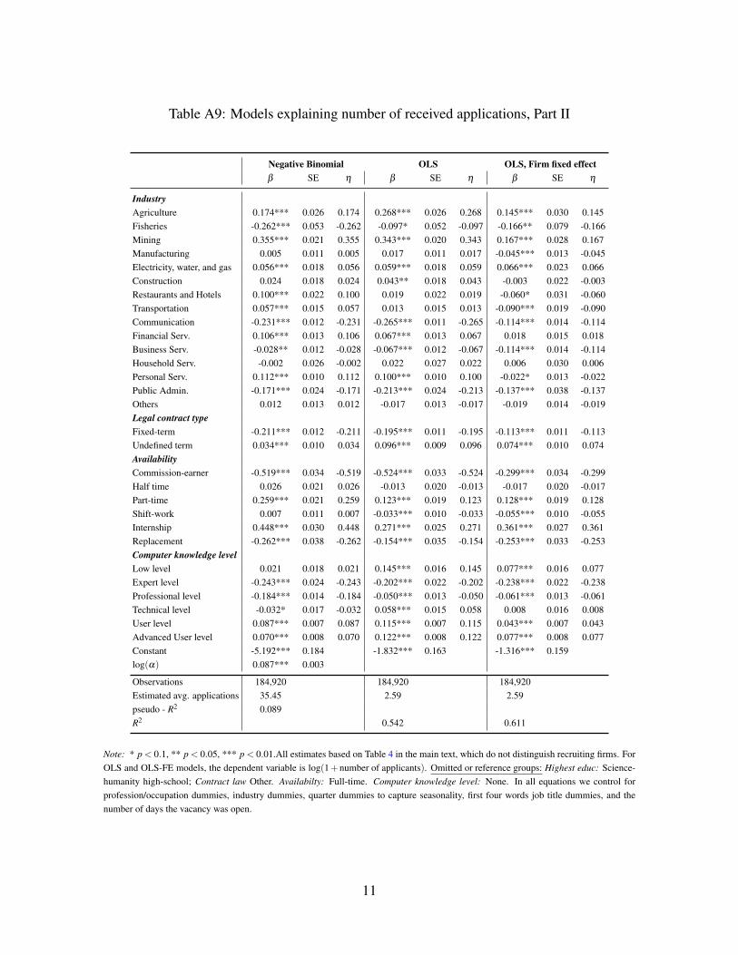
Table A9: Models explaining number of received applications, Part II

Negative Binomial OLS OLS, Firm fixed effectβ SE η β SE η β SE η

IndustryAgriculture 0.174*** 0.026 0.174 0.268*** 0.026 0.268 0.145*** 0.030 0.145Fisheries -0.262*** 0.053 -0.262 -0.097* 0.052 -0.097 -0.166** 0.079 -0.166Mining 0.355*** 0.021 0.355 0.343*** 0.020 0.343 0.167*** 0.028 0.167Manufacturing 0.005 0.011 0.005 0.017 0.011 0.017 -0.045*** 0.013 -0.045Electricity, water, and gas 0.056*** 0.018 0.056 0.059*** 0.018 0.059 0.066*** 0.023 0.066Construction 0.024 0.018 0.024 0.043** 0.018 0.043 -0.003 0.022 -0.003Restaurants and Hotels 0.100*** 0.022 0.100 0.019 0.022 0.019 -0.060* 0.031 -0.060Transportation 0.057*** 0.015 0.057 0.013 0.015 0.013 -0.090*** 0.019 -0.090Communication -0.231*** 0.012 -0.231 -0.265*** 0.011 -0.265 -0.114*** 0.014 -0.114Financial Serv. 0.106*** 0.013 0.106 0.067*** 0.013 0.067 0.018 0.015 0.018Business Serv. -0.028** 0.012 -0.028 -0.067*** 0.012 -0.067 -0.114*** 0.014 -0.114Household Serv. -0.002 0.026 -0.002 0.022 0.027 0.022 0.006 0.030 0.006Personal Serv. 0.112*** 0.010 0.112 0.100*** 0.010 0.100 -0.022* 0.013 -0.022Public Admin. -0.171*** 0.024 -0.171 -0.213*** 0.024 -0.213 -0.137*** 0.038 -0.137Others 0.012 0.013 0.012 -0.017 0.013 -0.017 -0.019 0.014 -0.019Legal contract typeFixed-term -0.211*** 0.012 -0.211 -0.195*** 0.011 -0.195 -0.113*** 0.011 -0.113Undefined term 0.034*** 0.010 0.034 0.096*** 0.009 0.096 0.074*** 0.010 0.074AvailabilityCommission-earner -0.519*** 0.034 -0.519 -0.524*** 0.033 -0.524 -0.299*** 0.034 -0.299Half time 0.026 0.021 0.026 -0.013 0.020 -0.013 -0.017 0.020 -0.017Part-time 0.259*** 0.021 0.259 0.123*** 0.019 0.123 0.128*** 0.019 0.128Shift-work 0.007 0.011 0.007 -0.033*** 0.010 -0.033 -0.055*** 0.010 -0.055Internship 0.448*** 0.030 0.448 0.271*** 0.025 0.271 0.361*** 0.027 0.361Replacement -0.262*** 0.038 -0.262 -0.154*** 0.035 -0.154 -0.253*** 0.033 -0.253Computer knowledge levelLow level 0.021 0.018 0.021 0.145*** 0.016 0.145 0.077*** 0.016 0.077Expert level -0.243*** 0.024 -0.243 -0.202*** 0.022 -0.202 -0.238*** 0.022 -0.238Professional level -0.184*** 0.014 -0.184 -0.050*** 0.013 -0.050 -0.061*** 0.013 -0.061Technical level -0.032* 0.017 -0.032 0.058*** 0.015 0.058 0.008 0.016 0.008User level 0.087*** 0.007 0.087 0.115*** 0.007 0.115 0.043*** 0.007 0.043Advanced User level 0.070*** 0.008 0.070 0.122*** 0.008 0.122 0.077*** 0.008 0.077Constant -5.192*** 0.184 -1.832*** 0.163 -1.316*** 0.159log(α) 0.087*** 0.003

Observations 184,920 184,920 184,920Estimated avg. applications 35.45 2.59 2.59pseudo - R2 0.089R2 0.542 0.611

Note: * p < 0.1, ** p < 0.05, *** p < 0.01.All estimates based on Table 4 in the main text, which do not distinguish recruiting firms. ForOLS and OLS-FE models, the dependent variable is log(1+number of applicants). Omitted or reference groups: Highest educ: Science-humanity high-school; Contract law Other. Availabilty: Full-time. Computer knowledge level: None. In all equations we control forprofession/occupation dummies, industry dummies, quarter dummies to capture seasonality, first four words job title dummies, and thenumber of days the vacancy was open.

11

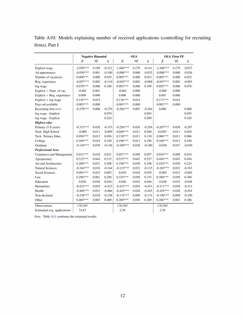
Table A10: Models explaining number of received applications (controlling for recruiting

firms), Part I

Negative Binomial OLS OLS, Firm FEβ SE η β SE η β SE η

Explicit wage -2.030*** 0.189 -0.121 -1.666*** 0.179 -0.141 -2.268*** 0.179 -0.037Ad appearances -0.030*** 0.001 -0.100 -0.008*** 0.000 -0.025 -0.008*** 0.000 -0.026Number of vacancies 0.008*** 0.000 0.039 0.005*** 0.000 0.023 0.005*** 0.000 0.022Req. experience -0.057*** 0.002 -0.110 -0.045*** 0.002 -0.088 -0.047*** 0.002 -0.093log wage 0.079*** 0.006 0.100 0.093*** 0.006 0.109 0.055*** 0.006 0.078Explicit × Num. of vac. -0.001 0.001 -0.001 0.000 -0.000 0.000Explicit × Req. experience 0.009 0.006 0.008 0.006 0.001 0.006Explicit × log wage 0.145*** 0.015 0.116*** 0.014 0.171*** 0.014Days ad available 0.003*** 0.000 0.003*** 0.000 0.002*** 0.000Recruiting firm (=1) -0.270*** 0.008 -0.270 -0.284*** 0.007 -0.284 0.000 . 0.000log wage - Implicit 0.079 0.093 0.055log wage - Explicit 0.224 0.209 0.226Highest educPrimary (1-8 years) -0.333*** 0.028 -0.333 -0.256*** 0.026 -0.256 -0.287*** 0.028 -0.287Tech. High School -0.009 0.011 -0.009 0.048*** 0.011 0.048 0.020* 0.011 0.020Tech. Tertiary Educ. 0.056*** 0.012 0.056 0.130*** 0.011 0.130 0.086*** 0.011 0.086College 0.169*** 0.014 0.169 0.196*** 0.013 0.196 0.160*** 0.013 0.160Graduate -0.136*** 0.039 -0.136 -0.100*** 0.038 -0.100 -0.030 0.037 -0.030Professional AreaCommerce and Management 0.031*** 0.010 0.031 0.057*** 0.009 0.057 0.034*** 0.009 0.034Agropecuary 0.515*** 0.044 0.515 0.537*** 0.042 0.537 0.494*** 0.043 0.494Art and Architecture 0.288*** 0.031 0.288 0.198*** 0.030 0.198 0.224*** 0.030 0.224Natural Sciences -0.164*** 0.034 -0.164 -0.115*** 0.032 -0.115 -0.183*** 0.032 -0.183Social Sciences 0.093*** 0.023 0.093 0.039 0.024 0.039 -0.005 0.023 -0.005Law 0.296*** 0.061 0.296 0.335*** 0.059 0.335 0.380*** 0.059 0.380Education 0.030 0.038 0.030 0.046 0.035 0.046 -0.038 0.035 -0.038Humanities -0.423*** 0.055 -0.423 -0.433*** 0.054 -0.433 -0.311*** 0.058 -0.311Health -0.466*** 0.031 -0.466 -0.445*** 0.028 -0.445 -0.454*** 0.028 -0.454Non-declared -0.238*** 0.010 -0.238 -0.174*** 0.009 -0.174 -0.190*** 0.009 -0.190Other 0.469*** 0.065 0.469 0.269*** 0.056 0.269 0.286*** 0.061 0.286

Observations 170,365 170,365 170,365Estimated avg. applications 34.87 2.59 2.59

Note: Table A11 continues the estimated results.

12

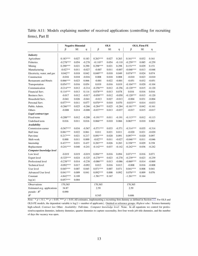
Table A11: Models explaining number of received applications (controlling for recruiting

firms), Part II

Negative Binomial OLS OLS, Firm FEβ SE η β SE η β SE η

IndustryAgriculture 0.183*** 0.027 0.183 0.263*** 0.027 0.263 0.161*** 0.032 0.161Fisheries -0.278*** 0.054 -0.278 -0.110** 0.054 -0.110 -0.259*** 0.085 -0.259Mining 0.290*** 0.021 0.290 0.298*** 0.021 0.298 0.151*** 0.029 0.151Manufacturing -0.027** 0.011 -0.027 -0.007 0.011 -0.007 -0.048*** 0.013 -0.048Electricity, water, and gas 0.042** 0.018 0.042 0.049*** 0.018 0.049 0.074*** 0.024 0.074Construction -0.016 0.018 -0.016 0.008 0.018 0.008 -0.010 0.023 -0.010Restaurants and Hotels 0.066*** 0.023 0.066 -0.001 0.022 -0.001 -0.051 0.032 -0.051Transportation 0.054*** 0.016 0.054 0.019 0.016 0.019 -0.104*** 0.020 -0.104Communication -0.214*** 0.012 -0.214 -0.256*** 0.012 -0.256 -0.120*** 0.015 -0.120Financial Serv. 0.114*** 0.013 0.114 0.078*** 0.013 0.078 0.016 0.016 0.016Business Serv. -0.017 0.012 -0.017 -0.050*** 0.012 -0.050 -0.120*** 0.015 -0.120Household Serv. -0.041 0.026 -0.041 -0.013 0.027 -0.013 -0.004 0.031 -0.004Personal Serv. 0.077*** 0.011 0.077 0.070*** 0.010 0.070 -0.033** 0.014 -0.033Public Admin. -0.266*** 0.025 -0.266 -0.284*** 0.025 -0.284 -0.161*** 0.042 -0.161Others -0.008 0.014 -0.008 -0.037*** 0.013 -0.037 -0.017 0.015 -0.017Legal contract typeFixed-term -0.208*** 0.012 -0.208 -0.191*** 0.011 -0.191 -0.113*** 0.012 -0.113Undefined term 0.016 0.011 0.016 0.066*** 0.010 0.066 0.065*** 0.010 0.065AvailabilityCommission-earner -0.567*** 0.034 -0.567 -0.571*** 0.033 -0.571 -0.314*** 0.035 -0.314Half time 0.061*** 0.022 0.061 0.011 0.021 0.011 -0.020 0.021 -0.020Part-time 0.217*** 0.021 0.217 0.091*** 0.020 0.091 0.097*** 0.020 0.097Shift-work 0.000 0.011 0.000 -0.027** 0.011 -0.027 -0.046*** 0.011 -0.046Internship 0.437*** 0.031 0.437 0.283*** 0.026 0.283 0.358*** 0.029 0.358Replacement -0.241*** 0.040 -0.241 -0.142*** 0.037 -0.142 -0.242*** 0.036 -0.242Computer knowledge levelLow level -0.019 0.019 -0.019 0.094*** 0.016 0.094 0.071*** 0.016 0.071Expert level -0.325*** 0.024 -0.325 -0.270*** 0.023 -0.270 -0.239*** 0.023 -0.239Professional level -0.238*** 0.014 -0.238 -0.086*** 0.013 -0.086 -0.069*** 0.014 -0.069Technical level -0.092*** 0.017 -0.092 0.013 0.016 0.013 -0.008 0.016 -0.008User level 0.045*** 0.007 0.045 0.071*** 0.007 0.071 0.041*** 0.008 0.041Advanced User level 0.041*** 0.009 0.041 0.092*** 0.008 0.092 0.076*** 0.009 0.076Constant -4.842*** 0.189 -1.581*** 0.167 -1.261*** 0.164log(α) 0.057*** 0.004

Observations 170,365 170,365 170,365Estimated avg. applications 34.87 2.59 2.59pseudo - R2 0.090R2 0.545 0.606

Note: * p < 0.1, ** p < 0.05, *** p < 0.01.All estimates, implementing a recruiting firm dummy as defined in Section 2.2. For OLS andOLS-FE models, the dependent variable is log(1+ number of applicants). Omitted or reference groups: Highest educ: Science-humanityhigh-school; Contract law Other. Availabilty: Full-time. Computer knowledge level: None. In all equations we control for profes-sion/occupation dummies, industry dummies, quarter dummies to capture seasonality, first four words job title dummies, and the numberof days the vacancy was open.

13

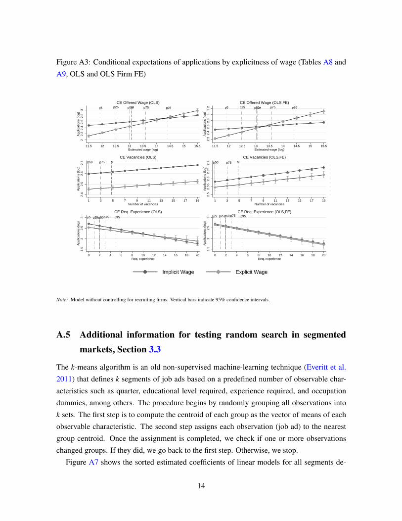
Figure A3: Conditional expectations of applications by explicitness of wage (Tables A8 and

A9, OLS and OLS Firm FE)

p5 p25 p50 p75 p95M

22.

22.

42.

62.

83

App

licat

ions

(lo

g)

11.5 12 12.5 13 13.5 14 14.5 15 15.5Estimated wage (log)

CE Offered Wage (OLS)

p5 p25 p50 p75M

p5 p25 p50M p75 p95

2.2

2.4

2.6

2.8

33.

2A

pplic

atio

ns (

log)

11.5 12 12.5 13 13.5 14 14.5 15 15.5Estimated wage (log)

CE Offered Wage (OLS,FE)

p5p25p50 p75 M

p50 p75 M

2.4

2.5

2.6

2.7

App

licat

ions

(lo

g)

1 3 5 7 9 11 13 15 17 19Number of vacancies

CE Vacancies (OLS)

p5p25p50 p75 M

p50 p75 M

2.5

2.55

2.6

2.65

2.7

App

licat

ions

(lo

g)1 3 5 7 9 11 13 15 17 19

Number of vacancies

CE Vacancies (OLS,FE)

p5 p25p50p75 p95

1.5

22.

53

App

licat

ions

(lo

g)

0 2 4 6 8 10 12 14 16 18 20Req. experience

CE Req. Experience (OLS)p5 p25p50 p75 p95

1.5

22.

53

App

licat

ions

(lo

g)

0 2 4 6 8 10 12 14 16 18 20Req. experience

CE Req. Experience (OLS,FE)

Implicit Wage Explicit Wage

Note: Model without controlling for recruiting firms. Vertical bars indicate 95% confidence intervals.

A.5 Additional information for testing random search in segmentedmarkets, Section 3.3

The k-means algorithm is an old non-supervised machine-learning technique (Everitt et al.

2011) that defines k segments of job ads based on a predefined number of observable char-

acteristics such as quarter, educational level required, experience required, and occupation

dummies, among others. The procedure begins by randomly grouping all observations into

k sets. The first step is to compute the centroid of each group as the vector of means of each

observable characteristic. The second step assigns each observation (job ad) to the nearest

group centroid. Once the assignment is completed, we check if one or more observations

changed groups. If they did, we go back to the first step. Otherwise, we stop.

Figure A7 shows the sorted estimated coefficients of linear models for all segments de-

14

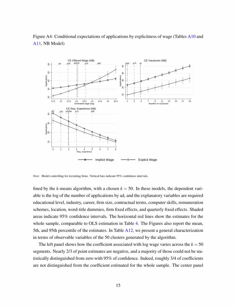
Figure A4: Conditional expectations of applications by explicitness of wage (Tables A10 and

A11, NB Model)

p5 p25 p50 p75M

p5 p25 p50M p75 p95

2030

4050

60A

pplic

atio

ns

11.5 12 12.5 13 13.5 14 14.5 15 15.5Estimated wage (log)

CE Offered Wage (NB)

p5p25p50 p75 M

p50 p75 M

3234

3638

40A

pplic

atio

ns

1 3 5 7 9 11 13 15 17 19Number of vacancies

CE Vacancies (NB)

p5 p25 p50/M p75 p95

2530

3540

App

licat

ions

0 1 2 3 4 5 6 7 8Req. experience

CE Req. Experience (NB)

Implicit Wage Explicit Wage

Note: Model controlling for recruiting firms. Vertical bars indicate 95% confidence intervals.

fined by the k-means algorithm, with a chosen k = 50. In these models, the dependent vari-

able is the log of the number of applications by ad, and the explanatory variables are required

educational level, industry, career, firm size, contractual terms, computer skills, remuneration

schemes, location, word-title dummies, firm fixed effects, and quarterly fixed effects. Shaded

areas indicate 95% confidence intervals. The horizontal red lines show the estimates for the

whole sample, comparable to OLS estimation in Table 4. The Figures also report the mean,

5th, and 95th percentile of the estimates. In Table A12, we present a general characterization

in terms of observable variables of the 50 clusters generated by the algorithm.

The left panel shows how the coefficient associated with log wage varies across the k = 50

segments. Nearly 2/3 of point estimates are negative, and a majority of those could not be sta-

tistically distinguished from zero with 95% of confidence. Indeed, roughly 3/4 of coefficients

are not distinguished from the coefficient estimated for the whole sample. The center panel

15

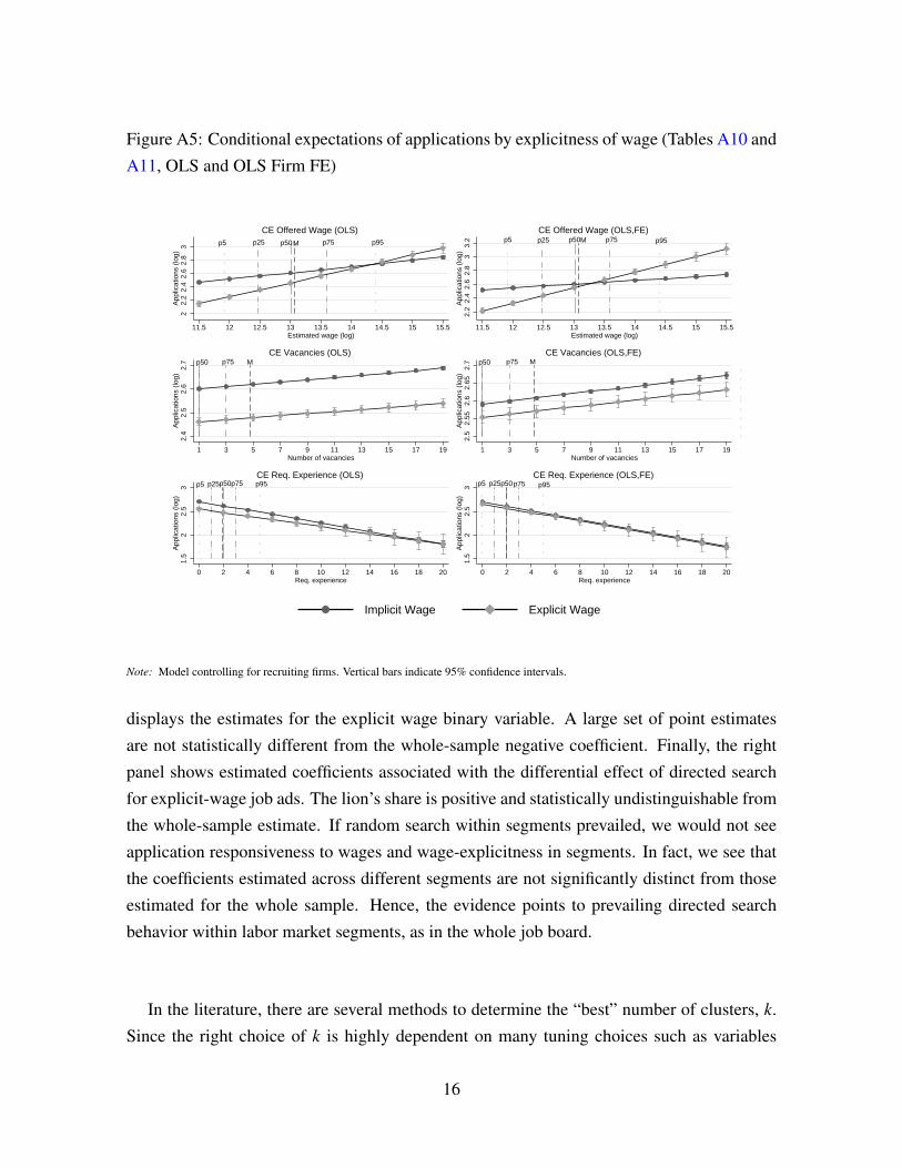
Figure A5: Conditional expectations of applications by explicitness of wage (Tables A10 and

A11, OLS and OLS Firm FE)

p5 p25 p50 p75M

p5 p25 p50M p75 p95

22.

22.

42.

62.

83

App

licat

ions

(lo

g)

11.5 12 12.5 13 13.5 14 14.5 15 15.5Estimated wage (log)

CE Offered Wage (OLS)

p5 p25 p50 p75M

p5 p25 p50M p75 p95

2.2

2.4

2.6

2.8

33.

2A

pplic

atio

ns (

log)

11.5 12 12.5 13 13.5 14 14.5 15 15.5Estimated wage (log)

CE Offered Wage (OLS,FE)

p5p25p50 p75 M

p50 p75 M

2.4

2.5

2.6

2.7

App

licat

ions

(lo

g)

1 3 5 7 9 11 13 15 17 19Number of vacancies

CE Vacancies (OLS)

p5p25p50 p75 M

p50 p75 M

2.5

2.55

2.6

2.65

2.7

App

licat

ions

(lo

g)1 3 5 7 9 11 13 15 17 19

Number of vacancies

CE Vacancies (OLS,FE)

p5 p25p50p75 p95

1.5

22.

53

App

licat

ions

(lo

g)

0 2 4 6 8 10 12 14 16 18 20Req. experience

CE Req. Experience (OLS)p5 p25p50p75 p95

1.5

22.

53

App

licat

ions

(lo

g)

0 2 4 6 8 10 12 14 16 18 20Req. experience

CE Req. Experience (OLS,FE)

Implicit Wage Explicit Wage

Note: Model controlling for recruiting firms. Vertical bars indicate 95% confidence intervals.

displays the estimates for the explicit wage binary variable. A large set of point estimates

are not statistically different from the whole-sample negative coefficient. Finally, the right

panel shows estimated coefficients associated with the differential effect of directed search

for explicit-wage job ads. The lion’s share is positive and statistically undistinguishable from

the whole-sample estimate. If random search within segments prevailed, we would not see

application responsiveness to wages and wage-explicitness in segments. In fact, we see that

the coefficients estimated across different segments are not significantly distinct from those

estimated for the whole sample. Hence, the evidence points to prevailing directed search

behavior within labor market segments, as in the whole job board.

In the literature, there are several methods to determine the “best” number of clusters, k.

Since the right choice of k is highly dependent on many tuning choices such as variables

16

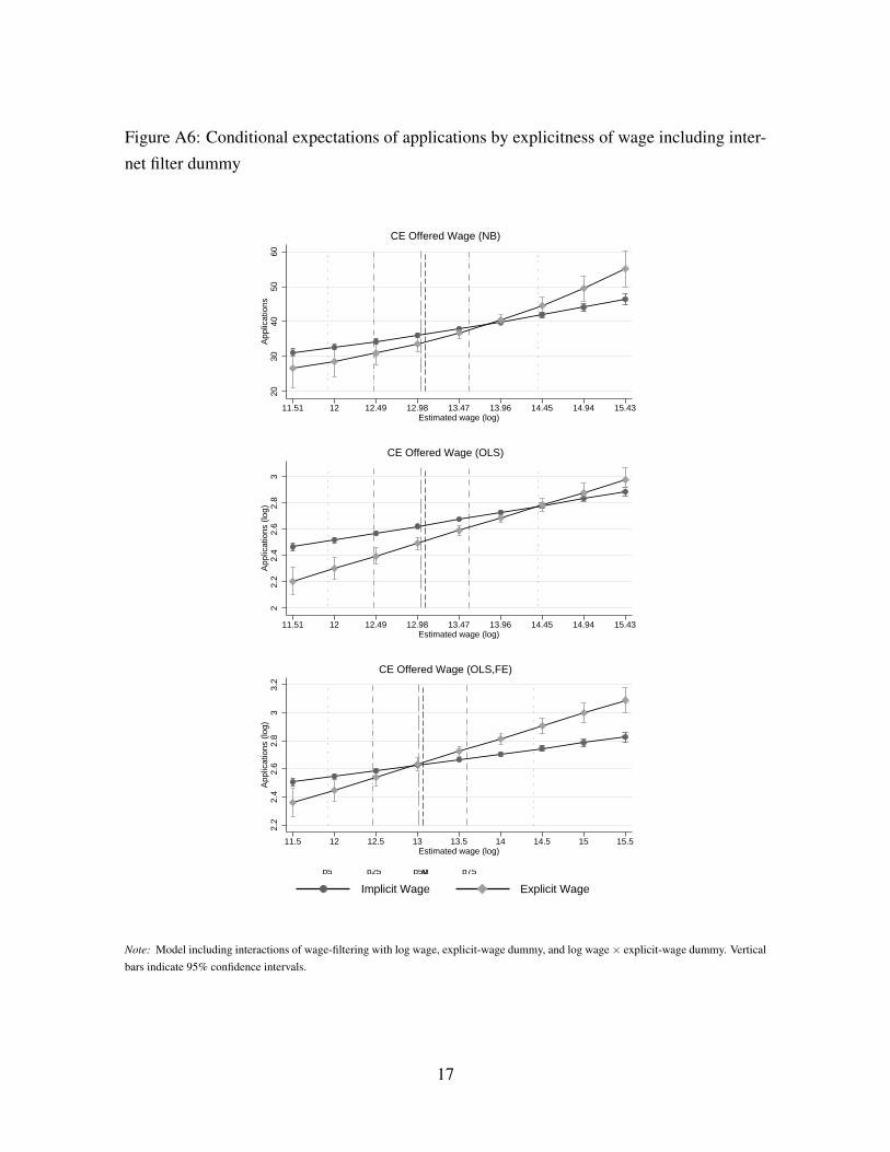
Figure A6: Conditional expectations of applications by explicitness of wage including inter-

net filter dummy

p5 p25 p50 p75M

2030

4050

60A

pplic

atio

ns

11.51 12 12.49 12.98 13.47 13.96 14.45 14.94 15.43Estimated wage (log)

CE Offered Wage (NB)

p5 p25 p50 p75M

22.

22.

42.

62.

83

App

licat

ions

(lo

g)

11.51 12 12.49 12.98 13.47 13.96 14.45 14.94 15.43Estimated wage (log)

CE Offered Wage (OLS)

p5 p25 p50 p75M

2.2

2.4

2.6

2.8

33.

2A

pplic

atio

ns (

log)

11.5 12 12.5 13 13.5 14 14.5 15 15.5Estimated wage (log)

CE Offered Wage (OLS,FE)

Implicit Wage Explicit Wage

Note: Model including interactions of wage-filtering with log wage, explicit-wage dummy, and log wage× explicit-wage dummy. Verticalbars indicate 95% confidence intervals.

17

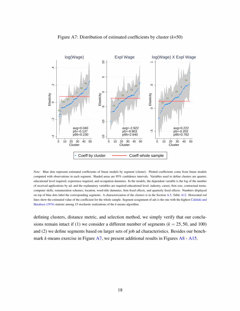
Figure A7: Distribution of estimated coefficients by cluster (k=50)

43

1547

2

3

48

40

-.4

-.2

0.2

.4E

last

icity

0 10 20 30 40 50Cluster

avg=0.040p5=-0.137p95=0.230

log(Wage)

14

6

26

113

42

-15

-10

-50

510

Ela

stic

ity

0 10 20 30 40 50Cluster

avg=-2.922p5=-9.903p95=2.640

Expl Wage

42

131

26

6

14

-.5

0.5

1E

last

icity

0 10 20 30 40 50Cluster

avg=0.222p5=-0.202p95=0.762

log(Wage) X Expl Wage

Coeff by cluster Coeff whole sample

Note: Blue dots represent estimated coefficients of linear models by segment (cluster). Plotted coefficients come from linear modelscomputed with observations in each segment. Shaded areas are 95% confidence intervals. Variables used to define clusters are quarter,educational level required, experience required, and occupation dummies. In the models, the dependent variable is the log of the numberof received applications by ad, and the explanatory variables are required educational level, industry, career, firm size, contractual terms,computer skills, remuneration schemes, location, word-title dummies, firm fixed effects, and quarterly fixed effects. Numbers displayedon top of blue dots label the corresponding segments. A characterization of the clusters is in the Section A.5, Table A12. Horizontal redlines show the estimated value of the coefficient for the whole sample. Segment assignment of ads is the one with the highest Calinski andHarabasz (1974) statistic among 15 stochastic realizations of the k-means algorithm.

defining clusters, distance metric, and selection method, we simply verify that our conclu-

sions remain intact if (1) we consider a different number of segments (k = 25,50, and 100)

and (2) we define segments based on larger sets of job ad characteristics. Besides our bench-

mark k-means exercise in Figure A7, we present additional results in Figures A8 - A15.

18

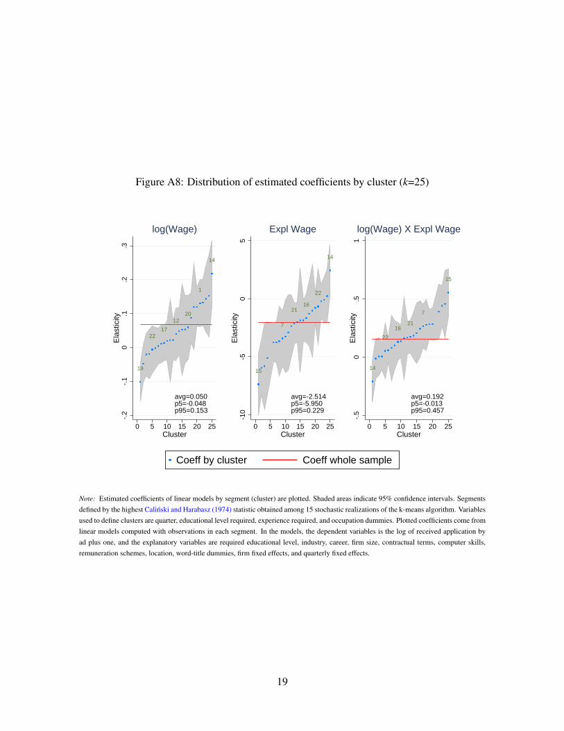
Figure A8: Distribution of estimated coefficients by cluster (k=25)

19

2217

1220

1

14

-.2

-.1

0.1

.2.3

Ela

stic

ity

0 5 10 15 20 25Cluster

avg=0.050p5=-0.048p95=0.153

log(Wage)

15

7

2116

22

14

-10

-50

5E

last

icity

0 5 10 15 20 25Cluster

avg=-2.514p5=-5.950p95=0.229

Expl Wage

14

22

1621

7

15

-.5

0.5

1E

last

icity

0 5 10 15 20 25Cluster

avg=0.192p5=-0.013p95=0.457

log(Wage) X Expl Wage

Coeff by cluster Coeff whole sample

Note: Estimated coefficients of linear models by segment (cluster) are plotted. Shaded areas indicate 95% confidence intervals. Segmentsdefined by the highest Calinski and Harabasz (1974) statistic obtained among 15 stochastic realizations of the k-means algorithm. Variablesused to define clusters are quarter, educational level required, experience required, and occupation dummies. Plotted coefficients come fromlinear models computed with observations in each segment. In the models, the dependent variables is the log of received application byad plus one, and the explanatory variables are required educational level, industry, career, firm size, contractual terms, computer skills,remuneration schemes, location, word-title dummies, firm fixed effects, and quarterly fixed effects.

19

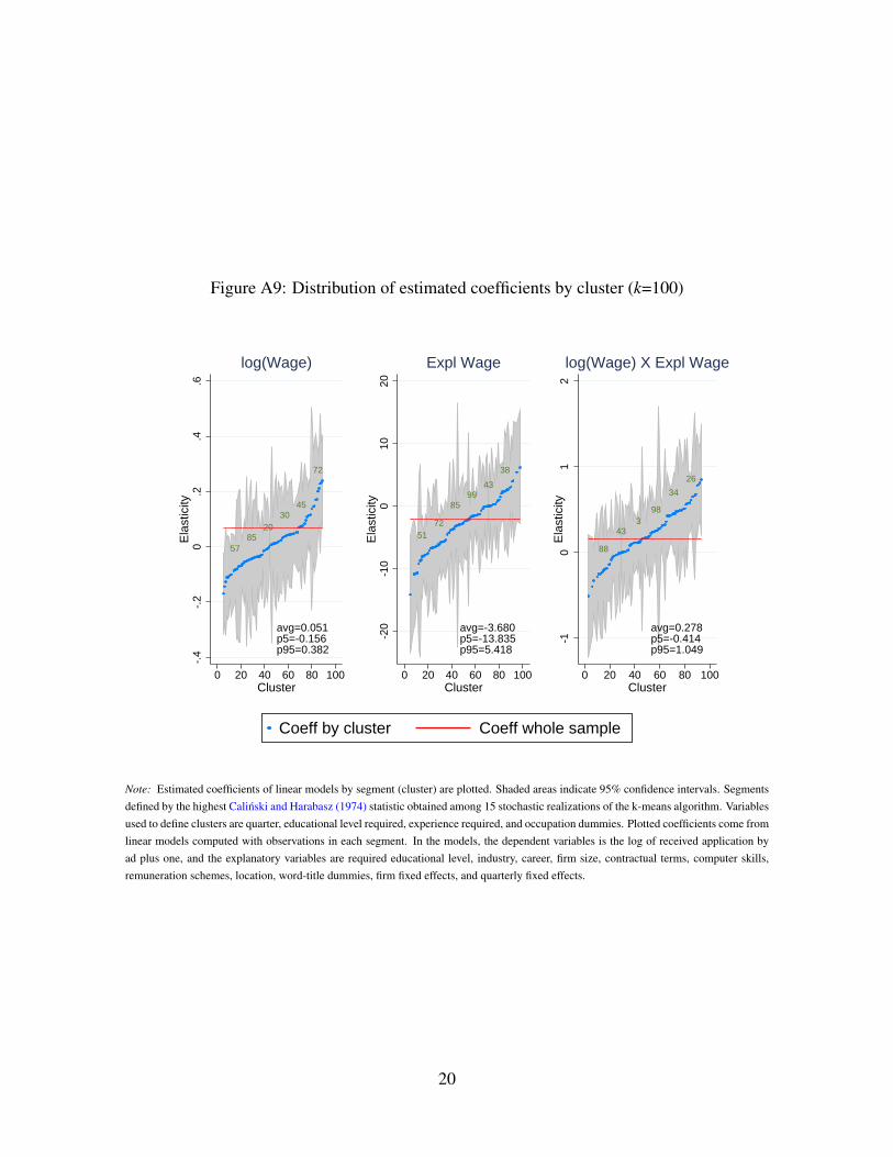
Figure A9: Distribution of estimated coefficients by cluster (k=100)

5785

2030

45

72

-.4

-.2

0.2

.4.6

Ela

stic

ity

0 20 40 60 80 100Cluster

avg=0.051p5=-0.156p95=0.382

log(Wage)

5172

8599

43

38

-20

-10

010

20E

last

icity

0 20 40 60 80 100Cluster

avg=-3.680p5=-13.835p95=5.418

Expl Wage

88

433

98

34

26

-10

12

Ela

stic

ity

0 20 40 60 80 100Cluster

avg=0.278p5=-0.414p95=1.049

log(Wage) X Expl Wage

Coeff by cluster Coeff whole sample

Note: Estimated coefficients of linear models by segment (cluster) are plotted. Shaded areas indicate 95% confidence intervals. Segmentsdefined by the highest Calinski and Harabasz (1974) statistic obtained among 15 stochastic realizations of the k-means algorithm. Variablesused to define clusters are quarter, educational level required, experience required, and occupation dummies. Plotted coefficients come fromlinear models computed with observations in each segment. In the models, the dependent variables is the log of received application byad plus one, and the explanatory variables are required educational level, industry, career, firm size, contractual terms, computer skills,remuneration schemes, location, word-title dummies, firm fixed effects, and quarterly fixed effects.

20

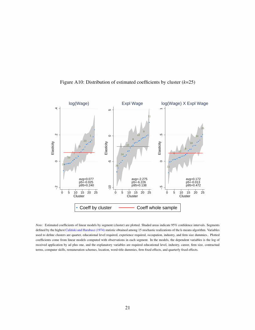
Figure A10: Distribution of estimated coefficients by cluster (k=25)

24

13

7

3

23

1

-.2

0.2

.4E

last

icity

0 5 10 15 20 25Cluster

avg=0.077p5=-0.025p95=0.240

log(Wage)

25

24

10

8

129

11

-10

-50

5E

last

icity

0 5 10 15 20 25Cluster

avg=-2.275p5=-6.226p95=0.138

Expl Wage

11

612

8

18

24

25

-.5

0.5

1E

last

icity

0 5 10 15 20 25Cluster

avg=0.172p5=-0.013p95=0.472

log(Wage) X Expl Wage

Coeff by cluster Coeff whole sample

Note: Estimated coefficients of linear models by segment (cluster) are plotted. Shaded areas indicate 95% confidence intervals. Segmentsdefined by the highest Calinski and Harabasz (1974) statistic obtained among 15 stochastic realizations of the k-means algorithm. Variablesused to define clusters are quarter, educational level required, experience required, occupation, industry, and firm size dummies.. Plottedcoefficients come from linear models computed with observations in each segment. In the models, the dependent variables is the log ofreceived application by ad plus one, and the explanatory variables are required educational level, industry, career, firm size, contractualterms, computer skills, remuneration schemes, location, word-title dummies, firm fixed effects, and quarterly fixed effects.

21

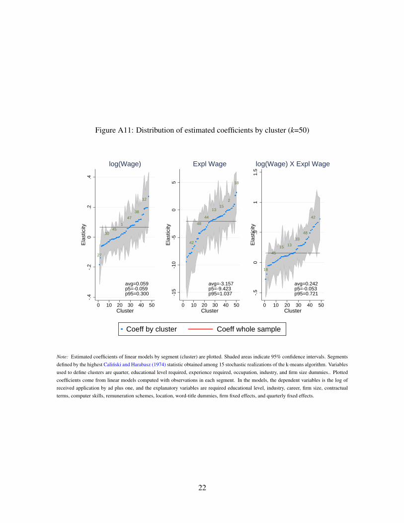
Figure A11: Distribution of estimated coefficients by cluster (k=50)

27

3045

1

47

38

12

-.4

-.2

0.2

.4E

last

icity

0 10 20 30 40 50Cluster

avg=0.059p5=-0.059p95=0.300

log(Wage)

42

48

44

1315

2

18

-15

-10

-50

5E

last

icity

0 10 20 30 40 50Cluster

avg=-3.157p5=-9.423p95=1.037

Expl Wage

18

45

15 13

33

48

42

-.5

0.5

11.

5E

last

icity

0 10 20 30 40 50Cluster

avg=0.242p5=-0.053p95=0.721

log(Wage) X Expl Wage

Coeff by cluster Coeff whole sample

Note: Estimated coefficients of linear models by segment (cluster) are plotted. Shaded areas indicate 95% confidence intervals. Segmentsdefined by the highest Calinski and Harabasz (1974) statistic obtained among 15 stochastic realizations of the k-means algorithm. Variablesused to define clusters are quarter, educational level required, experience required, occupation, industry, and firm size dummies.. Plottedcoefficients come from linear models computed with observations in each segment. In the models, the dependent variables is the log ofreceived application by ad plus one, and the explanatory variables are required educational level, industry, career, firm size, contractualterms, computer skills, remuneration schemes, location, word-title dummies, firm fixed effects, and quarterly fixed effects.

22

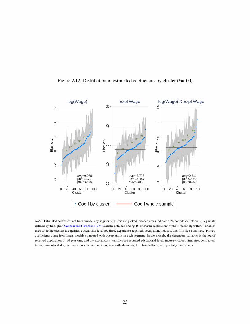
Figure A12: Distribution of estimated coefficients by cluster (k=100)

7727

1038

83

7

-.4

-.2

0.2

.4.6

Ela

stic

ity

0 20 40 60 80 100Cluster

avg=0.070p5=-0.132p95=0.429

log(Wage)

17

61

330

8619

-20

-10

010

20E

last

icity

0 20 40 60 80 100Cluster

avg=-2.793p5=-13.457p95=5.353

Expl Wage

93

94

31100

61

98

-1-.

50

.51

1.5

Ela

stic

ity

0 20 40 60 80 100Cluster

avg=0.211p5=-0.430p95=0.997

log(Wage) X Expl Wage

Coeff by cluster Coeff whole sample

Note: Estimated coefficients of linear models by segment (cluster) are plotted. Shaded areas indicate 95% confidence intervals. Segmentsdefined by the highest Calinski and Harabasz (1974) statistic obtained among 15 stochastic realizations of the k-means algorithm. Variablesused to define clusters are quarter, educational level required, experience required, occupation, industry, and firm size dummies.. Plottedcoefficients come from linear models computed with observations in each segment. In the models, the dependent variables is the log ofreceived application by ad plus one, and the explanatory variables are required educational level, industry, career, firm size, contractualterms, computer skills, remuneration schemes, location, word-title dummies, firm fixed effects, and quarterly fixed effects.

23

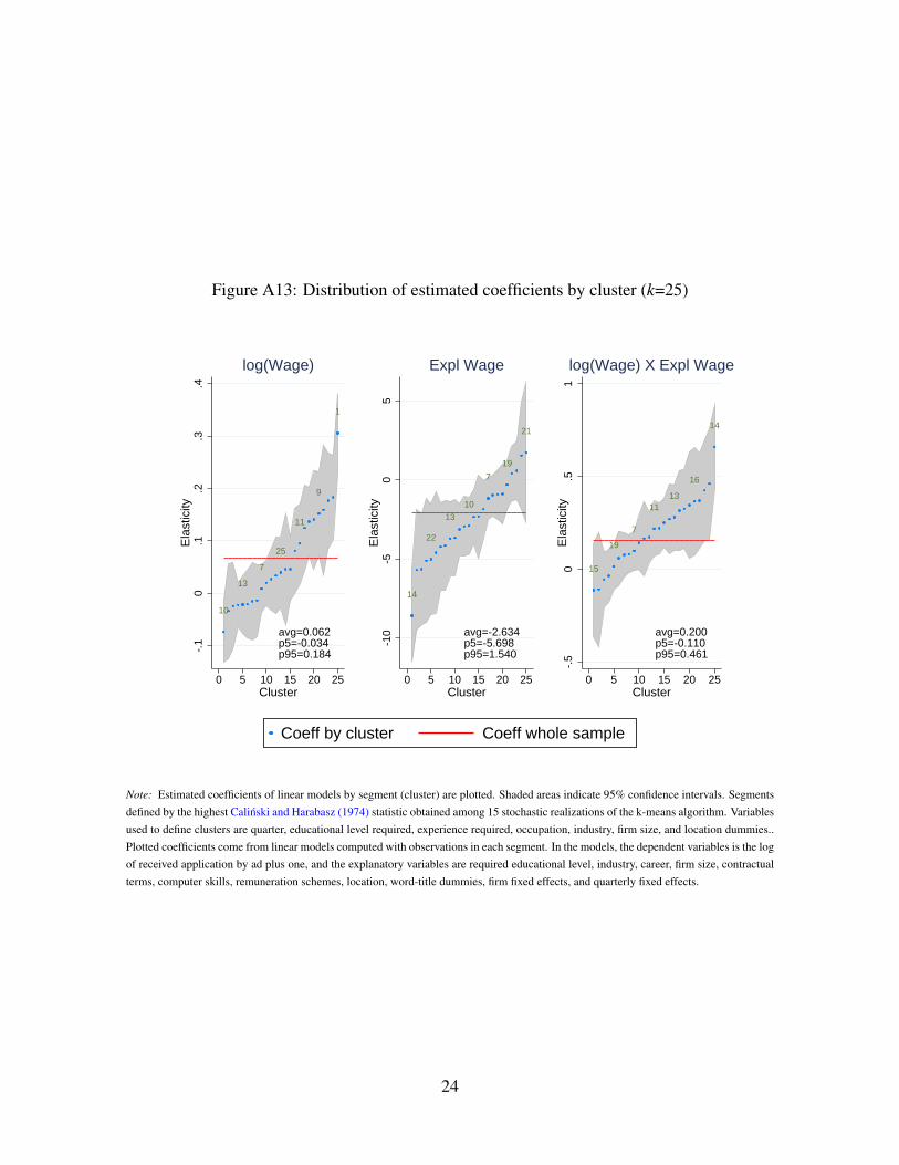
Figure A13: Distribution of estimated coefficients by cluster (k=25)

10

13

7

25

11

9

1

-.1

0.1

.2.3

.4E

last

icity

0 5 10 15 20 25Cluster

avg=0.062p5=-0.034p95=0.184

log(Wage)

14

22

13

10

7

19

21

-10

-50

5E

last

icity

0 5 10 15 20 25Cluster

avg=-2.634p5=-5.698p95=1.540

Expl Wage

15

19

7

1113

16

14

-.5

0.5

1E

last

icity

0 5 10 15 20 25Cluster

avg=0.200p5=-0.110p95=0.461

log(Wage) X Expl Wage

Coeff by cluster Coeff whole sample

Note: Estimated coefficients of linear models by segment (cluster) are plotted. Shaded areas indicate 95% confidence intervals. Segmentsdefined by the highest Calinski and Harabasz (1974) statistic obtained among 15 stochastic realizations of the k-means algorithm. Variablesused to define clusters are quarter, educational level required, experience required, occupation, industry, firm size, and location dummies..Plotted coefficients come from linear models computed with observations in each segment. In the models, the dependent variables is the logof received application by ad plus one, and the explanatory variables are required educational level, industry, career, firm size, contractualterms, computer skills, remuneration schemes, location, word-title dummies, firm fixed effects, and quarterly fixed effects.

24

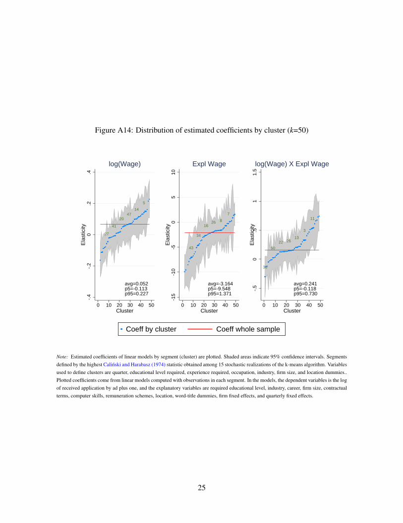
Figure A14: Distribution of estimated coefficients by cluster (k=50)

27

41

2047

14

5

-.4

-.2

0.2

.4E

last

icity

0 10 20 30 40 50Cluster

avg=0.052p5=-0.113p95=0.227

log(Wage)

43

34

1626 8

7

-15

-10

-50

510

Ela

stic

ity

0 10 20 30 40 50Cluster

avg=-3.164p5=-9.548p95=1.371

Expl Wage

36

50

22 2613

3

11

-.5

0.5

11.

5E

last

icity

0 10 20 30 40 50Cluster

avg=0.241p5=-0.118p95=0.730

log(Wage) X Expl Wage

Coeff by cluster Coeff whole sample

Note: Estimated coefficients of linear models by segment (cluster) are plotted. Shaded areas indicate 95% confidence intervals. Segmentsdefined by the highest Calinski and Harabasz (1974) statistic obtained among 15 stochastic realizations of the k-means algorithm. Variablesused to define clusters are quarter, educational level required, experience required, occupation, industry, firm size, and location dummies..Plotted coefficients come from linear models computed with observations in each segment. In the models, the dependent variables is the logof received application by ad plus one, and the explanatory variables are required educational level, industry, career, firm size, contractualterms, computer skills, remuneration schemes, location, word-title dummies, firm fixed effects, and quarterly fixed effects.

25

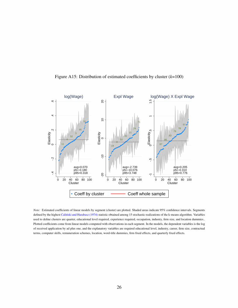
Figure A15: Distribution of estimated coefficients by cluster (k=100)

11

452

3

95

51

-.4

-.2

0.2

.4.6

Ela

stic

ity

0 20 40 60 80 100Cluster

avg=0.070p5=-0.180p95=0.318

log(Wage)

19

850

41

15

74

71

-20

-10

010

20E

last

icity

0 20 40 60 80 100Cluster

avg=-2.739p5=-10.076p95=3.748

Expl Wage

87

86

83

7578

67

-1-.

50

.51

1.5

Ela

stic

ity

0 20 40 60 80 100Cluster

avg=0.205p5=-0.310p95=0.776

log(Wage) X Expl Wage

Coeff by cluster Coeff whole sample

Note: Estimated coefficients of linear models by segment (cluster) are plotted. Shaded areas indicate 95% confidence intervals. Segmentsdefined by the highest Calinski and Harabasz (1974) statistic obtained among 15 stochastic realizations of the k-means algorithm. Variablesused to define clusters are quarter, educational level required, experience required, occupation, industry, firm size, and location dummies..Plotted coefficients come from linear models computed with observations in each segment. In the models, the dependent variables is the logof received application by ad plus one, and the explanatory variables are required educational level, industry, career, firm size, contractualterms, computer skills, remuneration schemes, location, word-title dummies, firm fixed effects, and quarterly fixed effects.

26

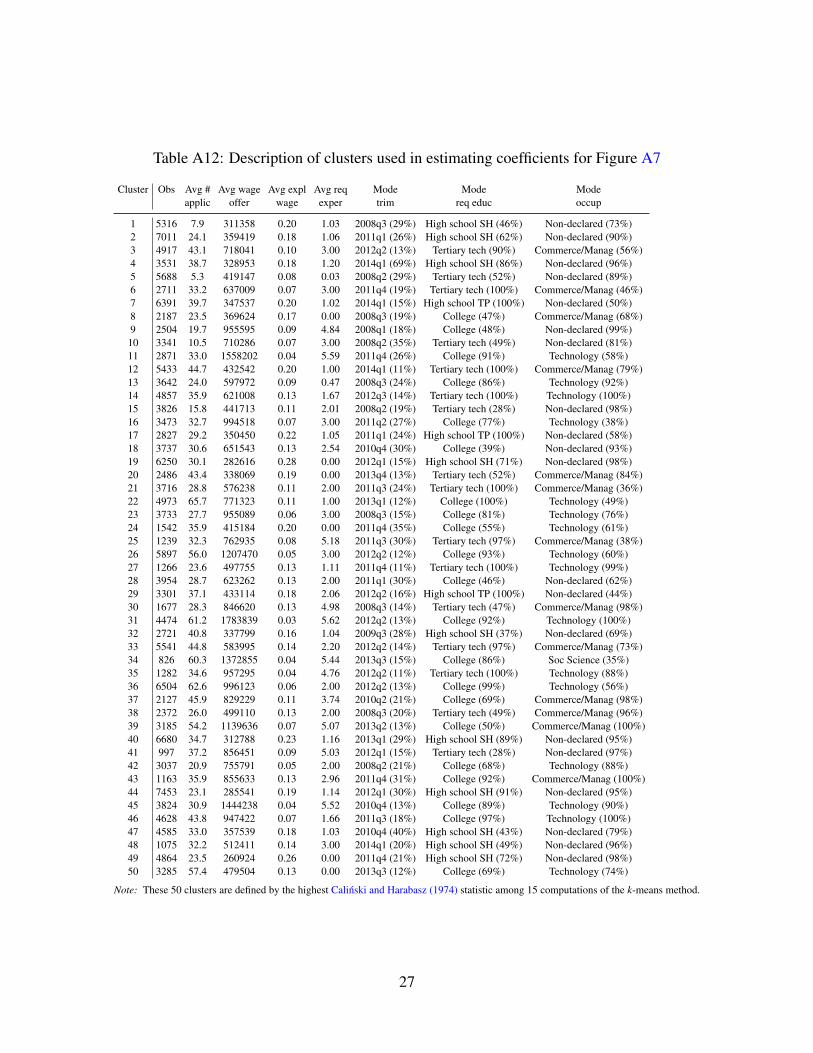
Table A12: Description of clusters used in estimating coefficients for Figure A7

Cluster Obs Avg # Avg wage Avg expl Avg req Mode Mode Modeapplic offer wage exper trim req educ occup

1 5316 7.9 311358 0.20 1.03 2008q3 (29%) High school SH (46%) Non-declared (73%)2 7011 24.1 359419 0.18 1.06 2011q1 (26%) High school SH (62%) Non-declared (90%)3 4917 43.1 718041 0.10 3.00 2012q2 (13%) Tertiary tech (90%) Commerce/Manag (56%)4 3531 38.7 328953 0.18 1.20 2014q1 (69%) High school SH (86%) Non-declared (96%)5 5688 5.3 419147 0.08 0.03 2008q2 (29%) Tertiary tech (52%) Non-declared (89%)6 2711 33.2 637009 0.07 3.00 2011q4 (19%) Tertiary tech (100%) Commerce/Manag (46%)7 6391 39.7 347537 0.20 1.02 2014q1 (15%) High school TP (100%) Non-declared (50%)8 2187 23.5 369624 0.17 0.00 2008q3 (19%) College (47%) Commerce/Manag (68%)9 2504 19.7 955595 0.09 4.84 2008q1 (18%) College (48%) Non-declared (99%)10 3341 10.5 710286 0.07 3.00 2008q2 (35%) Tertiary tech (49%) Non-declared (81%)11 2871 33.0 1558202 0.04 5.59 2011q4 (26%) College (91%) Technology (58%)12 5433 44.7 432542 0.20 1.00 2014q1 (11%) Tertiary tech (100%) Commerce/Manag (79%)13 3642 24.0 597972 0.09 0.47 2008q3 (24%) College (86%) Technology (92%)14 4857 35.9 621008 0.13 1.67 2012q3 (14%) Tertiary tech (100%) Technology (100%)15 3826 15.8 441713 0.11 2.01 2008q2 (19%) Tertiary tech (28%) Non-declared (98%)16 3473 32.7 994518 0.07 3.00 2011q2 (27%) College (77%) Technology (38%)17 2827 29.2 350450 0.22 1.05 2011q1 (24%) High school TP (100%) Non-declared (58%)18 3737 30.6 651543 0.13 2.54 2010q4 (30%) College (39%) Non-declared (93%)19 6250 30.1 282616 0.28 0.00 2012q1 (15%) High school SH (71%) Non-declared (98%)20 2486 43.4 338069 0.19 0.00 2013q4 (13%) Tertiary tech (52%) Commerce/Manag (84%)21 3716 28.8 576238 0.11 2.00 2011q3 (24%) Tertiary tech (100%) Commerce/Manag (36%)22 4973 65.7 771323 0.11 1.00 2013q1 (12%) College (100%) Technology (49%)23 3733 27.7 955089 0.06 3.00 2008q3 (15%) College (81%) Technology (76%)24 1542 35.9 415184 0.20 0.00 2011q4 (35%) College (55%) Technology (61%)25 1239 32.3 762935 0.08 5.18 2011q3 (30%) Tertiary tech (97%) Commerce/Manag (38%)26 5897 56.0 1207470 0.05 3.00 2012q2 (12%) College (93%) Technology (60%)27 1266 23.6 497755 0.13 1.11 2011q4 (11%) Tertiary tech (100%) Technology (99%)28 3954 28.7 623262 0.13 2.00 2011q1 (30%) College (46%) Non-declared (62%)29 3301 37.1 433114 0.18 2.06 2012q2 (16%) High school TP (100%) Non-declared (44%)30 1677 28.3 846620 0.13 4.98 2008q3 (14%) Tertiary tech (47%) Commerce/Manag (98%)31 4474 61.2 1783839 0.03 5.62 2012q2 (13%) College (92%) Technology (100%)32 2721 40.8 337799 0.16 1.04 2009q3 (28%) High school SH (37%) Non-declared (69%)33 5541 44.8 583995 0.14 2.20 2012q2 (14%) Tertiary tech (97%) Commerce/Manag (73%)34 826 60.3 1372855 0.04 5.44 2013q3 (15%) College (86%) Soc Science (35%)35 1282 34.6 957295 0.04 4.76 2012q2 (11%) Tertiary tech (100%) Technology (88%)36 6504 62.6 996123 0.06 2.00 2012q2 (13%) College (99%) Technology (56%)37 2127 45.9 829229 0.11 3.74 2010q2 (21%) College (69%) Commerce/Manag (98%)38 2372 26.0 499110 0.13 2.00 2008q3 (20%) Tertiary tech (49%) Commerce/Manag (96%)39 3185 54.2 1139636 0.07 5.07 2013q2 (13%) College (50%) Commerce/Manag (100%)40 6680 34.7 312788 0.23 1.16 2013q1 (29%) High school SH (89%) Non-declared (95%)41 997 37.2 856451 0.09 5.03 2012q1 (15%) Tertiary tech (28%) Non-declared (97%)42 3037 20.9 755791 0.05 2.00 2008q2 (21%) College (68%) Technology (88%)43 1163 35.9 855633 0.13 2.96 2011q4 (31%) College (92%) Commerce/Manag (100%)44 7453 23.1 285541 0.19 1.14 2012q1 (30%) High school SH (91%) Non-declared (95%)45 3824 30.9 1444238 0.04 5.52 2010q4 (13%) College (89%) Technology (90%)46 4628 43.8 947422 0.07 1.66 2011q3 (18%) College (97%) Technology (100%)47 4585 33.0 357539 0.18 1.03 2010q4 (40%) High school SH (43%) Non-declared (79%)48 1075 32.2 512411 0.14 3.00 2014q1 (20%) High school SH (49%) Non-declared (96%)49 4864 23.5 260924 0.26 0.00 2011q4 (21%) High school SH (72%) Non-declared (98%)50 3285 57.4 479504 0.13 0.00 2013q3 (12%) College (69%) Technology (74%)

Note: These 50 clusters are defined by the highest Calinski and Harabasz (1974) statistic among 15 computations of the k-means method.

27

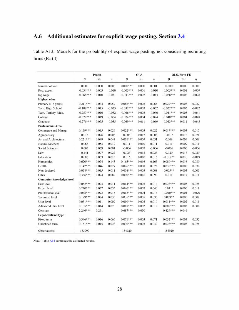
A.6 Additional estimates for explicit wage posting, Section 3.4

Table A13: Models for the probability of explicit wage posting, not considering recruiting

firms (Part I)

Probit OLS OLS, Firm FEβ SE η β SE η β SE η

Number of vac. 0.000 0.000 0.000 0.000*** 0.000 0.001 0.000 0.000 0.000Req. exper. -0.034*** 0.003 -0.010 -0.005*** 0.001 -0.010 -0.005*** 0.001 -0.009log wage -0.268*** 0.010 -0.051 -0.043*** 0.002 -0.043 -0.028*** 0.002 -0.028Highest educPrimary (1-8 years) 0.211*** 0.034 0.052 0.066*** 0.008 0.066 0.022*** 0.008 0.022Tech. High School -0.108*** 0.015 -0.023 -0.032*** 0.003 -0.032 -0.022*** 0.003 -0.022Tech. Tertiary Educ. -0.257*** 0.016 -0.052 -0.066*** 0.003 -0.066 -0.041*** 0.003 -0.041College -0.328*** 0.019 -0.064 -0.074*** 0.004 -0.074 -0.048*** 0.004 -0.048Graduate -0.276*** 0.075 -0.055 -0.069*** 0.011 -0.069 -0.043*** 0.011 -0.043Professional AreaCommerce and Manag. 0.139*** 0.015 0.026 0.022*** 0.003 0.022 0.017*** 0.003 0.017Agropecuary 0.015 0.076 0.003 0.008 0.012 0.008 0.021* 0.012 0.021Art and Architecture 0.221*** 0.049 0.044 0.031*** 0.009 0.031 0.009 0.009 0.009Natural Sciences 0.066 0.053 0.012 0.011 0.010 0.011 0.011 0.009 0.011Social Sciences 0.003 0.039 0.001 -0.006 0.007 -0.006 -0.006 0.006 -0.006Law 0.141 0.097 0.027 0.023 0.018 0.023 0.020 0.017 0.020Education 0.080 0.053 0.015 0.016 0.010 0.016 -0.019** 0.010 -0.019Humanities 0.620*** 0.074 0.145 0.165*** 0.016 0.165 0.080*** 0.016 0.080Health 0.142*** 0.046 0.027 0.026*** 0.008 0.026 0.030*** 0.008 0.030Non-declared 0.058*** 0.015 0.011 0.008*** 0.003 0.008 0.005** 0.003 0.005Other 0.386*** 0.074 0.082 0.090*** 0.016 0.090 0.011 0.017 0.011Computer knowledge levelLow level 0.062*** 0.023 0.011 0.014*** 0.005 0.014 0.028*** 0.005 0.028Expert level 0.270*** 0.037 0.055 0.040*** 0.007 0.040 0.011* 0.006 0.011Professional level 0.068*** 0.023 0.013 0.013*** 0.004 0.013 -0.020*** 0.004 -0.020Technical level 0.179*** 0.024 0.035 0.035*** 0.005 0.035 0.009** 0.005 0.009User level 0.051*** 0.011 0.009 0.010*** 0.002 0.010 0.011*** 0.002 0.011Advanced User level 0.105*** 0.014 0.020 0.018*** 0.002 0.018 0.008*** 0.002 0.008Constant 2.246*** 0.291 0.687*** 0.050 0.429*** 0.046Legal contract typeFixed-term 0.346*** 0.016 0.066 0.071*** 0.003 0.071 0.032*** 0.003 0.032Undefined term 0.161*** 0.015 0.028 0.030*** 0.003 0.030 0.026*** 0.003 0.026

Observations 183997 184920 184920

Note: Table A14 continues the estimated results.

28

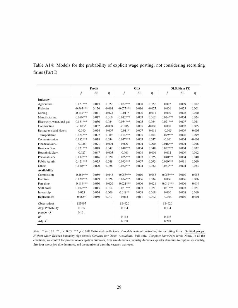
Table A14: Models for the probability of explicit wage posting, not considering recruiting

firms (Part I)

Probit OLS OLS, Firm FEβ SE η β SE η β SE η

IndustryAgriculture 0.121*** 0.043 0.022 0.022*** 0.008 0.022 0.012 0.009 0.012Fisheries -0.963*** 0.176 -0.094 -0.075*** 0.016 -0.075 0.001 0.023 0.001Mining -0.147*** 0.041 -0.023 -0.011* 0.006 -0.011 0.010 0.008 0.010Manufacturing 0.056*** 0.017 0.010 0.012*** 0.003 0.012 0.024*** 0.004 0.024Electricity, water, and gas 0.131*** 0.030 0.024 0.034*** 0.005 0.034 0.021*** 0.007 0.021Construction -0.053* 0.032 -0.009 -0.006 0.005 -0.006 0.005 0.007 0.005Restaurants and Hotels -0.040 0.034 -0.007 -0.011* 0.007 -0.011 -0.005 0.009 -0.005Transportation 0.424*** 0.022 0.089 0.104*** 0.005 0.104 0.099*** 0.006 0.099Communication 0.182*** 0.018 0.034 0.037*** 0.003 0.037 -0.001 0.004 -0.001Financial Serv. -0.026 0.021 -0.004 0.000 0.004 0.000 0.018*** 0.004 0.018Business Serv. 0.221*** 0.018 0.042 0.048*** 0.004 0.048 0.032*** 0.004 0.032Household Serv. -0.027 0.047 -0.005 -0.001 0.008 -0.001 0.012 0.009 0.012Personal Serv. 0.112*** 0.016 0.020 0.025*** 0.003 0.025 0.040*** 0.004 0.040Public Admin. 0.421*** 0.035 0.088 0.093*** 0.007 0.093 0.060*** 0.011 0.060Others 0.150*** 0.020 0.028 0.032*** 0.004 0.032 0.033*** 0.004 0.033AvailabilityCommission -0.264*** 0.059 -0.043 -0.053*** 0.010 -0.053 -0.058*** 0.010 -0.058Half time 0.129*** 0.029 0.026 0.034*** 0.006 0.034 0.006 0.006 0.006Part-time -0.114*** 0.030 -0.020 -0.021*** 0.006 -0.021 -0.019*** 0.006 -0.019Shift-work 0.072*** 0.015 0.014 0.021*** 0.003 0.021 0.021*** 0.003 0.021Internship 0.033 0.034 0.006 0.018** 0.008 0.018 0.010 0.008 0.010Replacement 0.085* 0.050 0.017 0.012 0.011 0.012 -0.004 0.010 -0.004

Observations 183997 184920 184920Avg. Probability 0.135 0.134 0.134pseudo - R2 0.131R2 0.113 0.316Adj. R2 0.109 0.289

Note: * p < 0.1, ** p < 0.05, *** p < 0.01.Estimated coefficients of models without controlling for recruiting firms. Omitted groups:Highest educ: Science-humanity high-school; Contract law Other. Availabilty: Full-time. Computer knowledge level: None. In all theequations, we control for profession/occupation dummies, firm size dummies, industry dummies, quarter dummies to capture seasonality,first four words job title dummies, and the number of days the vacancy was open.

29

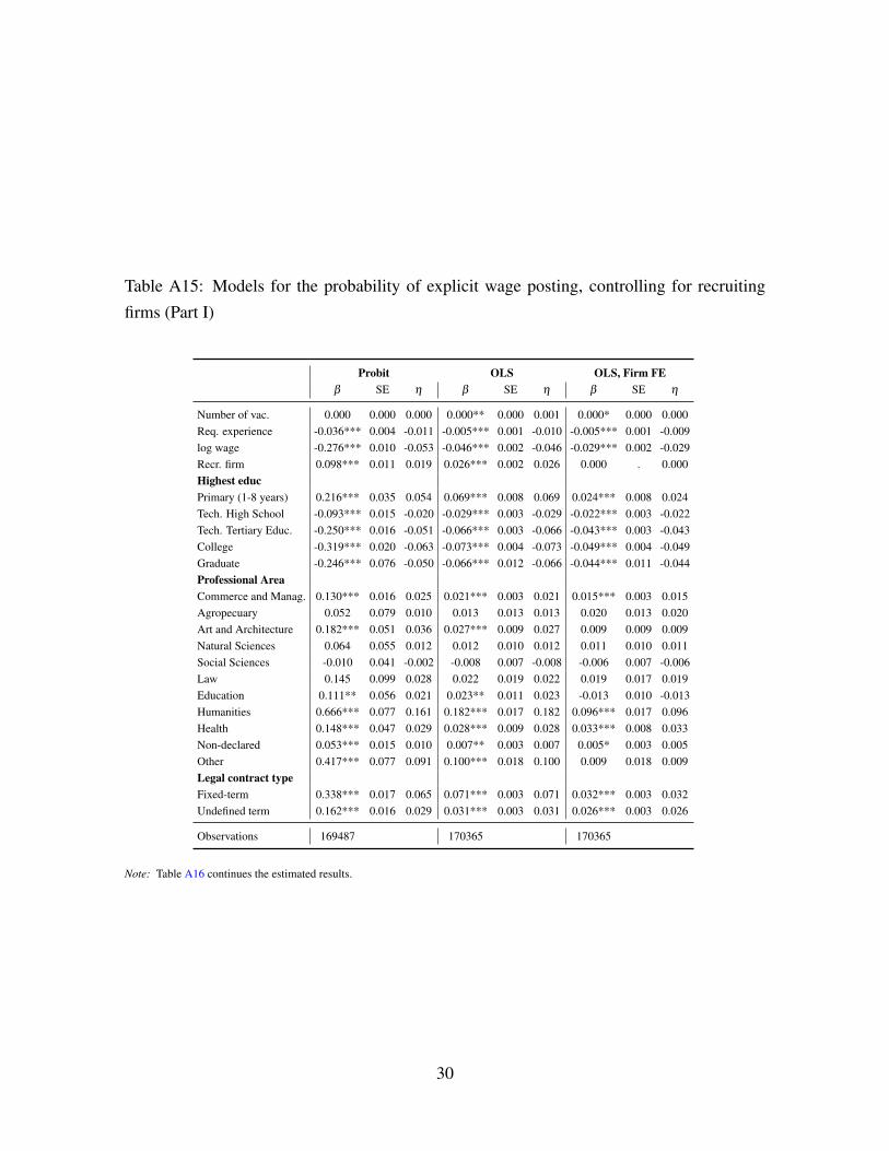
Table A15: Models for the probability of explicit wage posting, controlling for recruiting

firms (Part I)

Probit OLS OLS, Firm FEβ SE η β SE η β SE η

Number of vac. 0.000 0.000 0.000 0.000** 0.000 0.001 0.000* 0.000 0.000Req. experience -0.036*** 0.004 -0.011 -0.005*** 0.001 -0.010 -0.005*** 0.001 -0.009log wage -0.276*** 0.010 -0.053 -0.046*** 0.002 -0.046 -0.029*** 0.002 -0.029Recr. firm 0.098*** 0.011 0.019 0.026*** 0.002 0.026 0.000 . 0.000Highest educPrimary (1-8 years) 0.216*** 0.035 0.054 0.069*** 0.008 0.069 0.024*** 0.008 0.024Tech. High School -0.093*** 0.015 -0.020 -0.029*** 0.003 -0.029 -0.022*** 0.003 -0.022Tech. Tertiary Educ. -0.250*** 0.016 -0.051 -0.066*** 0.003 -0.066 -0.043*** 0.003 -0.043College -0.319*** 0.020 -0.063 -0.073*** 0.004 -0.073 -0.049*** 0.004 -0.049Graduate -0.246*** 0.076 -0.050 -0.066*** 0.012 -0.066 -0.044*** 0.011 -0.044Professional AreaCommerce and Manag. 0.130*** 0.016 0.025 0.021*** 0.003 0.021 0.015*** 0.003 0.015Agropecuary 0.052 0.079 0.010 0.013 0.013 0.013 0.020 0.013 0.020Art and Architecture 0.182*** 0.051 0.036 0.027*** 0.009 0.027 0.009 0.009 0.009Natural Sciences 0.064 0.055 0.012 0.012 0.010 0.012 0.011 0.010 0.011Social Sciences -0.010 0.041 -0.002 -0.008 0.007 -0.008 -0.006 0.007 -0.006Law 0.145 0.099 0.028 0.022 0.019 0.022 0.019 0.017 0.019Education 0.111** 0.056 0.021 0.023** 0.011 0.023 -0.013 0.010 -0.013Humanities 0.666*** 0.077 0.161 0.182*** 0.017 0.182 0.096*** 0.017 0.096Health 0.148*** 0.047 0.029 0.028*** 0.009 0.028 0.033*** 0.008 0.033Non-declared 0.053*** 0.015 0.010 0.007** 0.003 0.007 0.005* 0.003 0.005Other 0.417*** 0.077 0.091 0.100*** 0.018 0.100 0.009 0.018 0.009Legal contract typeFixed-term 0.338*** 0.017 0.065 0.071*** 0.003 0.071 0.032*** 0.003 0.032Undefined term 0.162*** 0.016 0.029 0.031*** 0.003 0.031 0.026*** 0.003 0.026

Observations 169487 170365 170365

Note: Table A16 continues the estimated results.

30

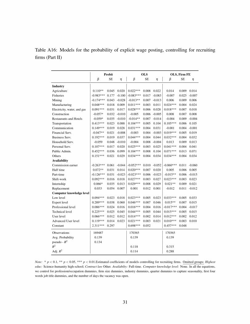
Table A16: Models for the probability of explicit wage posting, controlling for recruiting

firms (Part II)

Probit OLS OLS, Firm FEβ SE η β SE η β SE η

IndustryAgriculture 0.110** 0.045 0.020 0.022*** 0.008 0.022 0.014 0.009 0.014Fisheries -0.983*** 0.177 -0.100 -0.083*** 0.017 -0.083 -0.007 0.025 -0.007Mining -0.174*** 0.043 -0.028 -0.013** 0.007 -0.013 0.006 0.009 0.006Manufacturing 0.048*** 0.018 0.009 0.011*** 0.003 0.011 0.024*** 0.004 0.024Electricity, water, and gas 0.091*** 0.031 0.017 0.028*** 0.006 0.028 0.018*** 0.007 0.018Construction -0.057* 0.032 -0.010 -0.005 0.006 -0.005 0.008 0.007 0.008Restaurants and Hotels -0.059* 0.035 -0.010 -0.014** 0.007 -0.014 -0.004 0.009 -0.004Transportation 0.413*** 0.023 0.088 0.104*** 0.005 0.104 0.105*** 0.006 0.105Communication 0.149*** 0.019 0.028 0.031*** 0.004 0.031 -0.001 0.004 -0.001Financial Serv. -0.047** 0.021 -0.008 -0.003 0.004 -0.003 0.019*** 0.005 0.019Business Serv. 0.192*** 0.019 0.037 0.044*** 0.004 0.044 0.032*** 0.004 0.032Household Serv. -0.059 0.048 -0.010 -0.004 0.008 -0.004 0.013 0.009 0.013Personal Serv. 0.107*** 0.017 0.020 0.025*** 0.003 0.025 0.041*** 0.004 0.041Public Admin. 0.452*** 0.036 0.099 0.104*** 0.008 0.104 0.071*** 0.013 0.071Others 0.151*** 0.021 0.029 0.034*** 0.004 0.034 0.034*** 0.004 0.034AvailabilityCommission earner -0.263*** 0.061 -0.044 -0.052*** 0.010 -0.052 -0.060*** 0.011 -0.060Half time 0.072** 0.031 0.014 0.020*** 0.007 0.020 0.005 0.006 0.005Part-time -0.126*** 0.031 -0.023 -0.023*** 0.006 -0.023 -0.015** 0.006 -0.015Shift-work 0.092*** 0.016 0.018 0.027*** 0.003 0.027 0.023*** 0.003 0.023Internship 0.066* 0.035 0.013 0.029*** 0.008 0.029 0.021** 0.009 0.021Replacement 0.033 0.054 0.007 0.001 0.012 0.001 -0.012 0.011 -0.012Computer knowledge levelLow level 0.094*** 0.023 0.018 0.023*** 0.005 0.023 0.033*** 0.005 0.033Expert level 0.289*** 0.038 0.060 0.046*** 0.007 0.046 0.015** 0.007 0.015Professional level 0.086*** 0.024 0.016 0.016*** 0.004 0.016 -0.017*** 0.004 -0.017Technical level 0.225*** 0.025 0.045 0.044*** 0.005 0.044 0.015*** 0.005 0.015User level 0.066*** 0.012 0.012 0.014*** 0.002 0.014 0.012*** 0.002 0.012Advanced User level 0.119*** 0.014 0.023 0.021*** 0.003 0.021 0.010*** 0.003 0.010Constant 2.311*** 0.297 0.698*** 0.052 0.457*** 0.048

Observations 169487 170365 170365Avg. Probability 0.139 0.139 0.139pseudo - R2 0.134R2 0.118 0.315Adj. R2 0.114 0.288

Note: * p < 0.1, ** p < 0.05, *** p < 0.01.Estimated coefficients of models controlling for recruiting firms. Omitted groups: Highesteduc: Science-humanity high-school; Contract law Other. Availabilty: Full-time. Computer knowledge level: None. In all the equations,we control for profession/occupation dummies, firm size dummies, industry dummies, quarter dummies to capture seasonality, first fourwords job title dummies, and the number of days the vacancy was open.

31

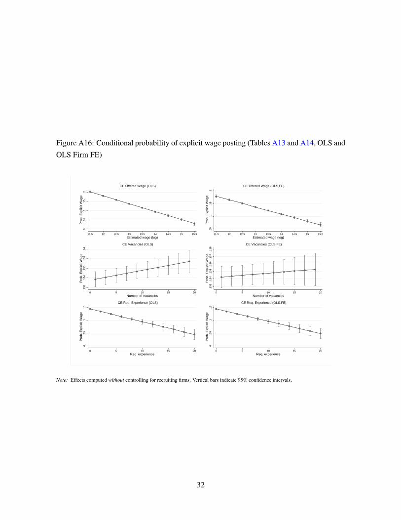
Figure A16: Conditional probability of explicit wage posting (Tables A13 and A14, OLS and

OLS Firm FE)

0.0

5.1

.15

.2P

rob.

Exp

licit

Wag

e

11.5 12 12.5 13 13.5 14 14.5 15 15.5Estimated wage (log)

CE Offered Wage (OLS)

.132

.134

.136

.138

.14

Pro

b. E

xplic

it W

age

0 5 10 15 20Number of vacancies

CE Vacancies (OLS)

0.0

5.1

.15

Pro

b. E

xplic

it W

age

0 5 10 15 20Req. experience

CE Req. Experience (OLS)

.05

.1.1

5.2

Pro

b. E

xplic

it W

age

11.5 12 12.5 13 13.5 14 14.5 15 15.5Estimated wage (log)

CE Offered Wage (OLS,FE)

.133

.134

.135

.136

.137

.138

Pro

b. E

xplic

it W

age

0 5 10 15 20Number of vacancies

CE Vacancies (OLS,FE)

0.0

5.1

.15

Pro

b. E

xplic

it W

age

0 5 10 15 20Req. experience

CE Req. Experience (OLS,FE)

Note: Effects computed without controlling for recruiting firms. Vertical bars indicate 95% confidence intervals.

32

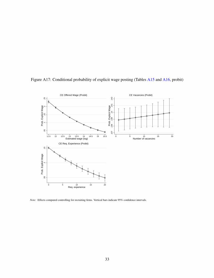
Figure A17: Conditional probability of explicit wage posting (Tables A15 and A16, probit)

.05

.1.1

5.2

.25

Pro

b. E

xplic

it W

age

11.5 12 12.5 13 13.5 14 14.5 15 15.5Estimated wage (log)

CE Offered Wage (Probit)

.137

.138

.139

.14

.141

.142

Pro

b. E

xplic

it W

age

0 5 10 15 20Number of vacancies

CE Vacancies (Probit)

.05

.1.1

5P

rob.

Exp

licit

Wag

e

0 5 10 15 20Req. experience

CE Req. Experience (Probit)

Note: Effects computed controlling for recruiting firms. Vertical bars indicate 95% confidence intervals.

33

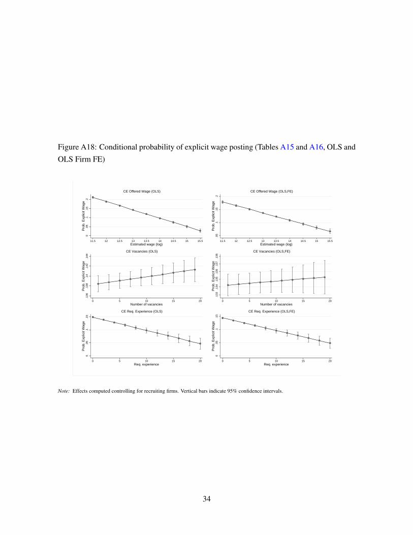
Figure A18: Conditional probability of explicit wage posting (Tables A15 and A16, OLS and

OLS Firm FE)

0.0

5.1

.15

.2P

rob.

Exp

licit

Wag

e

11.5 12 12.5 13 13.5 14 14.5 15 15.5Estimated wage (log)

CE Offered Wage (OLS)

.136

.138

.14

.142

.144

Pro

b. E

xplic

it W

age

0 5 10 15 20Number of vacancies

CE Vacancies (OLS)

0.0

5.1

.15

Pro

b. E

xplic

it W

age

0 5 10 15 20Req. experience

CE Req. Experience (OLS)

.05

.1.1

5.2

Pro

b. E

xplic

it W

age

11.5 12 12.5 13 13.5 14 14.5 15 15.5Estimated wage (log)

CE Offered Wage (OLS,FE)

.133

.134

.135

.136

.137

.138

Pro

b. E

xplic

it W

age

0 5 10 15 20Number of vacancies

CE Vacancies (OLS,FE)

0.0

5.1

.15

Pro

b. E

xplic

it W

age

0 5 10 15 20Req. experience

CE Req. Experience (OLS,FE)

Note: Effects computed controlling for recruiting firms. Vertical bars indicate 95% confidence intervals.

34

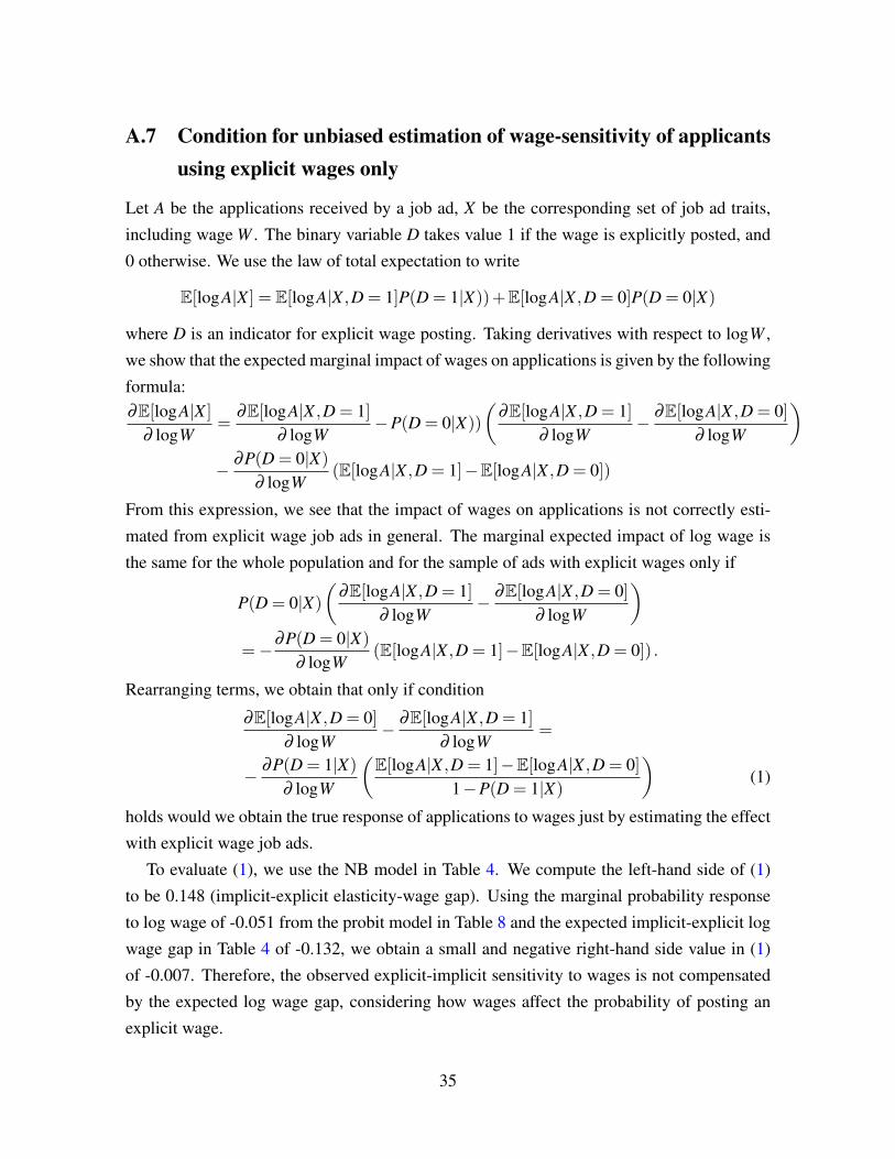
A.7 Condition for unbiased estimation of wage-sensitivity of applicantsusing explicit wages only

Let A be the applications received by a job ad, X be the corresponding set of job ad traits,

including wage W . The binary variable D takes value 1 if the wage is explicitly posted, and

0 otherwise. We use the law of total expectation to write

E[logA|X ] = E[logA|X ,D = 1]P(D = 1|X))+E[logA|X ,D = 0]P(D = 0|X)

where D is an indicator for explicit wage posting. Taking derivatives with respect to logW ,

we show that the expected marginal impact of wages on applications is given by the following

formula:∂E[logA|X ]

∂ logW=

∂E[logA|X ,D = 1]∂ logW

−P(D = 0|X))

(∂E[logA|X ,D = 1]

∂ logW− ∂E[logA|X ,D = 0]

∂ logW

)− ∂P(D = 0|X)

∂ logW(E[logA|X ,D = 1]−E[logA|X ,D = 0])

From this expression, we see that the impact of wages on applications is not correctly esti-

mated from explicit wage job ads in general. The marginal expected impact of log wage is

the same for the whole population and for the sample of ads with explicit wages only if

P(D = 0|X)

(∂E[logA|X ,D = 1]

∂ logW− ∂E[logA|X ,D = 0]

∂ logW

)=−∂P(D = 0|X)

∂ logW(E[logA|X ,D = 1]−E[logA|X ,D = 0]) .

Rearranging terms, we obtain that only if condition

∂E[logA|X ,D = 0]∂ logW

− ∂E[logA|X ,D = 1]∂ logW

=

− ∂P(D = 1|X)

∂ logW

(E[logA|X ,D = 1]−E[logA|X ,D = 0]

1−P(D = 1|X)

)(1)

holds would we obtain the true response of applications to wages just by estimating the effect

with explicit wage job ads.

To evaluate (1), we use the NB model in Table 4. We compute the left-hand side of (1)

to be 0.148 (implicit-explicit elasticity-wage gap). Using the marginal probability response

to log wage of -0.051 from the probit model in Table 8 and the expected implicit-explicit log

wage gap in Table 4 of -0.132, we obtain a small and negative right-hand side value in (1)

of -0.007. Therefore, the observed explicit-implicit sensitivity to wages is not compensated

by the expected log wage gap, considering how wages affect the probability of posting an

explicit wage.

35