Do Firms Share their Success with Workers? The Response of

Do Firms Share their Success with Workers?

The Response of Wages to Product Market

Conditions

Marcello Estevao and Stacey Tevlin∗

March 23, 2000

Abstract

We provide strong new evidence that industry financial conditions play an important rolein wage determination in the U.S. manufacturing sector. Ordinary least squares estimates ofthe effect of rents per worker on wages are positive and significant, but quite small. However,using two standard bargaining models, we illustrate that this may stem from a variety ofeconometric difficulties that plague the OLS estimates. In this paper, we are able to overcomethese issues and identify the effects of the industry financial situation on wages. We do thisusing the U.S. input-output tables to isolate exogenous variation in an industry’s productmarket conditions. Our instrumental variable estimates reveal a substantial amount of rentsharing in U.S. manufacturing—much more than is consistent with a purely competitivelabor market.

∗Economists, Division of Research and Statistics, Federal Reserve Board. Email: [email protected]. This paper

is a substantially revised version of FEDs working paper #95-48. We benefited from insightful discussions with

Joshua Angrist, Olivier Blanchard, Ricardo Caballero, Steve Pischke, Robert Solow and Beth Anne Wilson. We

are very grateful to the valuable suggestions provided by Lawrence Katz and two anonymous referees. We would

also like to thank seminar participants at MIT, University of Maryland, Iowa State University, and at the Federal

Reserve Board for their comments. We are responsible for all remaining errors and the views expressed do not

necessarily reflect the views of the Federal Reserve Board or any other members of its staff.

1 Introduction

One of the central aims of theoretical work on wage formation is to understand why wages fail

to clear the market for labor. Many of the theories that have been proposed to explain this

phenomenon imply a positive correlation between profits and wages. However, although empir-

ical studies on inter-industry wage differentials provide indirect evidence that such a correlation

may exist, direct tests of the effect of industry rents on wages in the US economy have yielded

very small estimates. The absence of direct empirical support casts doubt on the relevance of

industry performance in wage determination. In this paper, we provide strong direct evidence

that U.S. firms share rents with workers.

Previous studies of the US economy have been unable to find significant rent sharing

because—lacking appropriate instruments—they failed to overcome the endogeneity of firm

performance in a real wage equation. We use two simple bargaining models to illustrate that

the degree of rent sharing can be identified using instruments that shift the demand curve for

goods. By focusing on industries that are suppliers of intermediate inputs to other industries, we

are able to isolate exogenous demand shocks for 62 four-digit sectors. Our instrumental variable

analysis reveals that rent sharing is an important feature of the U.S. manufacturing sector. We

find an elasticity of wages with respect to firm performance that is ten times larger than OLS

estimates. This result is robust to changes in the sample period, the group of industries, and

the definition of industry performance, as well as to controls for worker quality.

This paper has five other sections. In the next section, we review the theoretical and em-

pirical literature on the relationship between wages and profits. Next, we present models that

provide a framework for the empirical section and, in particular, organize the discussion on

simultaneity and measurement error issues. Section 4 describes the empirical methodology to

be used, including the choice of instruments, the way we control for changes in the industry mix

of worker characteristics, and the specification of each variable used in the estimation. Section 5

reports results for different specifications of the basic equation relating real wages and rents.

The last section concludes.

2 The Literature

Several different theories predict a positive correlation between industry performance and wages.

Efficiency-wage theories predict that firms will choose not to cut wages because of the nega-

tive impact on productivity, and therefore, on profitability.1 Insider-outsider theories predict a

positive relationship between rents and wages because incumbent workers, or “insiders”, can be1The effect on productivity may stem from costly worker monitoring (Shapiro and Stiglitz (1984)) or labor

turnover costs (Salop (1979)). Akerlof and Yellen (1988) emphasize sociological and psychological reasons for

efficiency wages based on the idea of fairness.

2

uncooperative with new employees, or “outsiders”, causing adverse effects on overall produc-

tivity.2 These potential production disruptions are costlier to more profitable firms. A version

of the implicit contract models of Azariadis (1975) and Baily (1974) can also generate a pos-

itive relationship between wages and profits: As long as firms are not risk neutral, a positive

rent-sharing parameter is predicted because the derivative of wages with respect to profits is

positive and equal to the ratio of the relative risk aversion of firms to the relative risk aversion

of workers.3

According to all of these theories, firm-specific factors such as profitability and workers’

bargaining power are important determinants of the real wage paid to a worker and can be

used to explain inter-industry wage differentials.4 In contrast, under competitive labor market

conditions, these variables should not have explanatory power. If labor markets were truly

competitive, inter-industry wage differentials would have to be explained by differences in the

mix of worker characteristics across industries and/or by job compensating premia.

A series of studies using data from the U.S., the U.K., and Canada, has tested the relevance of

firm-specific variables in an equation for real wage determination. In general, the null hypothesis

of joint significance of these variables is not rejected, casting doubt on a purely competitive labor

market approach.5 Unfortunately, this approach yields results that are not robust to alternative

specifications. Each paper includes a different set of insider variables, and it is not clear what

the interpretation for each coefficient is.

An alternative approach is to align the equations with theory and provide a structural

interpretation for the coefficient on sectoral rent in a wage determination regression. Previous

authors that have employed this approach have found that the rent-sharing coefficient is positive

and significantly different from zero.6 Several of these papers use industry profits as a measure

of performance and find, in general, that the elasticity of real wages with respect to profits is

quite small. Sanfey (1992) estimates an elasticity of wages with respect to profits-per-worker

for the U.S. economy of .05, while Blanchflower et al (1996) estimate elasticities between .02

and .04. Studies that use data for other countries tend to find similarly small estimates.7

2See Lindbeck and Snower (1987) for a collection of papers in this tradition. The fundamentals of these models

give a rationale for the existence of unions that would be the institutional counterpart of insider power.3See Blanchflower et al (1996).4Nickell and Wadhwani (1990) and Nickell and Kong (1988) call these factors “insider variables”. The unem-

ployment rate, the average industrial wage, and unemployment insurance benefits would be examples of “outsider

variables”.5Dickens and Katz (1987) and Layard et al (1991) describe these results in detail.6For instance Blanchflower et al (1996), Carruth and Oswald (1990), Christofides and Oswald (1992), Currie

and McConnell (1992), Denny and Machin (1991), Gardner (1999), Hildreth and Oswald (1993), Nickell and

Wadhwani (1990), and Sanfey (1992).7We should note that some of these authors argue that these estimates are actually quite sizable. For instance,

Blanchflower et al (1996) point out that, according to their results, a 100 percent increase in profitability in an

industry would be associated with a pay rise of about 8 percent after some years. They argue that since profits

are a volatile series, an economically significant portion of wage dispersion can be explained by rents.

3

The main problem with these results is that they were produced without proper identifica-

tion of the rent-sharing parameter. The simultaneity between wages and financial conditions

generates inconsistent estimates of the elasticity of wages with respect to profitability mea-

sures. Controlling for this by using import and export prices as instrumental variables, Abowd

and Lemieux (1993) estimate a much higher elasticity for Canada (0.20). Similarly, using a

panel of U.K. firms and employing technological innovations as instruments, Van Reenen (1996)

estimates a rent-sharing coefficient of 0.29.

Although these two papers yield important evidence against the competitive labor market

paradigm, they do so for labor markets that are generally considered to be less competitive than

the U.S. market. Moreover, these studies use samples that are heavily unionized. (Indeed, the

Abowd-Lemieux sample consists entirely of collective bargaining agreements.) In addition, both

studies fail to control for changes in the industry composition of individual worker characteristics.

The Van Reenen study also is unable to control for variation in the number of hours worked.

In this paper, we extend this line of research to the U.S. labor market. We also control for

variations in worker quality and present alternative results taking into account the variation in

average hours worked.

The main reason that the instrumental variable approach has not been applied to U.S data

yet is that the instruments used in previous studies are either not applicable or unavailable for a

large economy like the U.S. Therefore, we introduce instruments that are new to this literature:

We use the input-output tables and the methods of Shea (1993) to select exogenous demand

shocks for a representative sample of U.S. industries. This method yields an elasticity of wages

per person with respect to rents per person (controlling for changes in labor quality) of about

0.29, implying that rent sharing is an important phenomenon in the U.S. economy.

3 Wages and rents

3.1 The basic estimation problem

In this section, we describe the basic problem of estimating rent sharing with ordinary least

squares. It is straightforward to show that OLS regressions of wages on various measures of

industry performance yield inconsistent estimates. Consider the following equation:

W = γR

N+ Z + η (1)

where W is the real wage (per worker); RN is real rents-per-worker; Z is a measure of the alter-

native wage a worker could expect to receive elsewhere; η represents relevant omitted variables;

and γ is the rent-sharing parameter. The estimation of equation (1) can be more or less problem-

atic depending on the measures of industry performance used. Accounting profits are commonly

used in the literature. Economic profits, which take into account depreciation allowances and

4

the rental cost of capital, are a better measure.8 However, the calculation of both definitions

of profits—subtracting the wage bill from value added—imparts a direct downward bias in γ

because W appears on both sides of the equation. In addition, the implicit assumptions under-

lying the calculation of economic profits lead to measurement error and inconsistent estimates

of γ. We choose to bypass profits altogether and use value added to measure industry rents. As

we will show, simple models of wage bargaining yield a structural relationship between value

added-per-worker and wages.

Unfortunately, value added may also be endogenous if, as seems likely, firms change labor

inputs in response to autonomous variations in wages. Moreover, value added may serve merely

as a proxy for the “true” financial variable that firms and workers bargain over. In this case, a

specification using value added could be plagued by measurement error. In the next section, we

present simple models that help illustrate these econometric difficulties and how we overcome

them. In particular, we derive identification conditions for the rent-sharing parameter using two

canonical bargaining models.

3.2 Bargaining models

Efficient bargaining. The first model assumes that workers and firms bargain over wages and

employment in order to maximize the joint surplus of their economic activity. If the parties do

not reach an agreement, they receive fallback incomes. Workers maximize the surplus expected

utility derived from their income (expected utility minus a threat point defined by the fallback

wage). The firm maximizes its surplus profits. We assume that the fallback or “strike” profit

is equal to zero. The source of workers’ bargaining power comes from their ability to act as a

group and is represented by the parameter µ.

The Nash bargaining process is summarized by the maximization of:

Ω = ΦµΠ1−µ (2)

where Π is the profit level of the firm. Φ is the surplus expected utility of a representative

worker, defined as:

Φ = N(v(W ) − v(Z)). (3)

W is the real wage; N is the level of employment hired by the firm; Z is the alternative wage;

and v(x) measures the utility derived by an individual from income x.

Equation (3) assumes that the alternative wage received by a dismissed worker is also the

fallback wage in case of a disagreement. Additionally, we choose the units of N so that N can be

interpreted as the probability of employment. The expected alternative wage, Z, is a function of

the representative worker’s characteristics–the “human capital” variables–and the state of the

economy, such as the unemployment rate and the magnitude of unemployment benefits.8See Blanchflower et al (1996), for instance.

5

Let us write profits as:

Π = Af(N) − WN

where A is a revenue-shifting parameter. This parameter will, in general, be a function of the

production technology and the demand for the final good. Af(N) is a value-added function

which here is assumed to be a function only of the amount of labor hired. Af(N) is the size

of the “pie” to be divided between employees and employers. In other words, after production

occurs and intermediate suppliers have been paid, the employer (who owns capital) bargains

with a representative employee (who owns labor) to determine how value added will be divided

between them.

The first-order conditions derived from maximizing (2) with respect to W and N are:

µAf(N)

N= (1 − µ)

v(W ) − v(Z)v′(W )

+ µW (4)

W = µAf(N)

N+ (1 − µ)Af ′(N) (5)

Linearizing v(Z) around W , omitting higher order terms, and rewriting both (4) and (5),

yields:

W = µAf(N)

N+ (1 − µ)Z (6)

Af ′(N) = Z (7)

This is the “strongly efficient” bargaining case. Wages are a weighted average of labor

productivity, Af(N)N , and the worker’s alternative market wage. The larger the bargaining power

of workers (µ) is, the larger wages are. When µ = 1, workers extract all the rents and firms

make zero profits. In this model, firms hire workers until marginal labor productivity, Af ′(N),

is equal to the wage a worker would receive if fired, Z. Therefore, the level of employment does

not depend on the contracted wage, implying that wage changes do not affect value added per

worker. Thus, in theory, equation (6) can be consistently estimated by ordinary least squares.

However, empirically, it may be difficult to accurately measure the financial conditions that

workers care about. Indeed, measurement error may be part of the reason that most authors

have found small estimates of the rent-sharing parameter. Fortunately, instrumental variables

which are correlated to industry rents but uncorrelated to the measurement error, can help us

uncover a consistent estimate of γ.

A right-to-manage model. The assumption that workers and firms bargain over both

wages and employment, as in the efficient bargaining model, has been criticized for being unre-

alistic. This assumption seems particularly heroic in the United States where wage negotiations

6

tend to be fairly decentralized. It seems likely that workers bargain over wages, but have no

voice in determining the overall level of employment.9 In the right-to-manage model, we allow

bargaining between workers and firms to reflect this inefficiency.

The Nash bargaining function to be maximized is now:

Ω = (N(W )(v(W ) − v(Z)))µΠ1−µ (8)

In (8 ), N(W ) represents the optimal number of workers an employer will choose given

the bargained level of wages. This function is obtained from the solution to the firm’s profit

maximization problem:

Af ′(N) = W (9)

Differentiating (8) with respect to W , using (9), and linearizing v(Z) around W , gives:

W = γAf(N)

N+ (1 − γ)Z (10)

γ = γ(µ, εfN , εWN ) (11)

According to equation (9), firms hire workers until the marginal product equals the con-

tracted wage, W , rather than the alternative wage, Z. Thus, firms take wage changes into

account when setting the level of employment, N . Therefore, this model points to an additional

reason that OLS estimates are inconsistent: Rents per worker will be endogenously determined.

Fortunately, as shown in equation (10), exogenous shifts in the revenue parameter, A—which

does not vary with the level of employment—would enable us to identify the rent-sharing coeffi-

cient, γ. Instrumental variables that are correlated to A, but not to autonomous variation in

wages, can help us with that task.

It is also interesting to note that because the settled wage affects the firm’s demand for

labor, the rent-sharing parameter, γ, is not only a function of the workers’ bargaining power,

but also of the elasticities of labor demand (εWN ) and the value added function (εfN ) with

respect to employment—both of which we assume to be constant. Therefore, in contrast to

the “efficient bargaining” model, γ is less than or equal to µ, the parameter that represents

workers’ bargaining power.10 Consequently, instrumental variables estimation generates a lower

bound for the parameter representing workers’ bargaining power. The larger the sensitivity of9Layard et al (1991), among others, present some evidence that this might be the case.

10After some algebra, it can be shown that γ = µ1−µεNW (1−εfN )/εfN

< µ, because εNW < 0 and 0 < εfN < 1

if the firm’s maximization problem has an interior maximum. If µ = 1, workers can set wages freely at a level,

say, W . If the result of firms’ profit maximization, taking W = W as given, generates positive profits, then

γ < µ = 1. However, if firms make negative profits when W = W , then workers would choose wages such that

profits are zero. In this case, γ = µ = 1. See also Abowd and Lemieux (1993) for an alternative discussion of the

relationship between γ and µ.

7

employment to changes in the contracted wage (i.e. the larger the magnitude of the elasticity

of labor demand), the larger the difference between γ and µ will be.

To summarize this section and the preceding one, OLS estimates may be inconsistent due to

measurement error in the regressor. Furthermore, if firms set the level of employment without

interference from workers, rents-per-worker will be highly endogenous. Fortunately, instrumen-

tal variables that shock the revenue parameter, A, help us overcome both problems and can be

used to consistently estimate γ.

4 Empirical methodology and data description

4.1 Demand-shifters

The last section made the case for the use of revenue-shifters as instruments for estimation of

rent-sharing equations. Either technology shocks or exogenous variations in the demand for

goods can be used as revenue shifters. We choose to use exogenous changes in demand for the

output of a particular industry as our revenue shifters.

We perform a panel data analysis for the four-digit sectors of U.S. manufacturing. One

way of obtaining good demand shifters for this database is to use the input-output approach

described in Shea (1993). Shea uses information from the input-output tables for two-, three-,

and four-digit industries to choose variables that should be correlated with demand shifts of

particular four-digit industries. Output of industry j is a good demand-shifter for industry i if

industry j demands a large share of industry i’s output, but industry i, and other sectors closely

related to it, comprise a small share of the production costs in industry j. The first condition

is to insure that output of industry j is relevant for identifying demand shifts. The second

condition is to minimize the possible sensitivity of the output of industry j to price variations in

industry i. In other words, the second condition guarantees exogeneity. Let us call the demand

share of industry j, DS, and the cost share of industry i, CS.

An example may help here. Consider the explosives industry (SIC 2892). About 19 percent

of the demand for explosives originates in the coal mining industry (SIC 12). However, the cost

of explosives comprises only 1 percent of the input costs that the coal mining industry incurs.

Thus, coal mining has the two characteristics that we want in an instrument: Movements in the

output of coal shift the demand curve for explosives, but coal output is unlikely to be affected

by conditions in the explosives industry. Therefore, coal mining is a good exogenous demand

shifter for the explosives industry.

Shea (1993) shows that the asymptotic bias in the IV estimates of the supply elasticity

obtained when using the input-output approach to select instruments is decreasing in the ratio,

DS/CS. For a given ratio, increases in DS should increase the correlation between final and

intermediate output. Using Monte-Carlo simulations, Shea shows that this increased correlation

improves the small sample behavior of his estimates over some range. Therefore, variables with

8

high DS/CS ratios are good demand-shifters, in the sense that they identify a supply elasticity

with small asymptotic bias. Since we need good demand-shifters, the same results apply to our

approach.11

This general rule is not enough to select potential instruments for industry i. It is also

important to impose rules on the process of instrument selection that minimize the influence of

common supply shocks between both the industry we use as an instrument and the industry for

which we need an instrument. For instance, the cost share data we use in instrument selection

is the cost share of the two-digit sector containing industry i. This guards against a situation

where the cost share is small merely because the four-digit industry is much smaller than the

two-digit instrument industry. In addition, we do not allow sectors with the same two-digit SIC

code as industry i to be instruments for industry i. This prohibition reflects the assumption that

supply shocks are highly correlated within a two-digit industry. For the same reason, industries

belonging to different SIC groups that are subject to similar supply shocks were not used as

instruments for one another.12

Instruments chosen by this approach are good proxies for exogenous variation in A, the

revenue-shifter: It is unlikely that variations in the price of sector i have a significant impact

on the output of sector j because the share of sector i in sector j’s cost is small. Industries

selected as demand-shifters according to this methodology tend to be more aggregated than the

industry for which we are instrumenting. Furthermore, some of the instruments could have been

considered good demand shocks even before we imposed restrictions to guarantee exogeneity.

Government defense spending is a good example. Changes in defense spending are primarily

related to political and social events, not to specific four-digit industry supply shocks.

After choosing instruments based upon the above criteria, we then checked the list of poten-

tial instruments to make sure that the correlation between the instrumental variable candidate

and the output of sector i was due to their input-output link. For instance, instrument candi-

dates were rejected if they were too closely related to business cycle variations because costs in

sector i could be correlated to the business cycle as well. To address this problem, we pretested

the potential instruments for relevance once business cycle variations were purged from the data.

First, we regressed the potential instruments on business cycle measures and saved the residuals

from this equation.13 Then we regressed output growth on the residual instrument growth to

check for instrument relevance. We discarded instruments which had low T ∗ R2 statistics or

were negatively correlated to the regressor.14 The 62 industries chosen after this final check was

concluded are reported in Appendix 1.11The threshold values we used are DS/CS > 3 and DS > 15 percent, the same as Shea used.12This is the case for the apparel and textile industries (SIC 23 and 22), the primary and fabricated metals

industries (SIC 33 and 34), and the industrial machinery and electrical machinery industries (SIC 35 and 36).13Different measures were used. The final regressions use total manufacturing price and production as business

cycle indicators. The results are insensitive to the choice of other indicators.14Although only a few instruments were negatively correlated to output, we discarded them since systematic

demand shocks should be related to variations in output in the same direction.

9

Some sectors have only one good instrument, while others have more than one. In order to

select one vector of instruments among all the available possibilities, we maximized the criterion

which is used to guarantee instrument exogeneity. Hence, we chose the instrument with the

highest ratio of DS to CS. These instruments are indicated by asterisks in the appendix. Using

multiple instruments where they are available or using other criteria to generate the demand-

shift vector generated nearly identical results to those reported in the next section.

4.2 Data and basic specification

Our dataset is drawn in large part from the NBER Productivity Database, which is constructed

using the Annual Survey of Manufactures.15 It includes annual data from 1958 to 1994. The

wage in industry i at time t, Wit, is computed as the ratio of total payroll to employment divided

by the consumer price index. The employment series, Nit, includes both production and non-

production workers. Real value added, Rit, is defined as the value of industry shipments plus

the change in inventories minus materials costs.16 Descriptive statistics for our key variables

are shown in Appendix 1.

We do not observe the alternative wage that a representative worker in a particular industry

would receive if fired and rehired in another industry. We assume that the alternative wage

will depend on three components: First, it will reflect the state of the aggregate labor market.

Second, it will depend on industry-specific factors such as the nature of the work and the

transferability of skills. These two components are easily controlled for using time dummies

and fixed effects. However, the third component, the human capital of employees, may not be.

Although a large portion of the differences in human capital across industry is likely captured

by fixed effects, the composition of workers and skills in an industry may change over time. This

requires a measure of human capital that varies across time and industry.

We construct our human capital measure, hcit, using household data from the Bureau of

Labor Statistics. Our method is described in detail in Appendix 3. Briefly, there are three main

steps: First using the outgoing rotation groups of the Current Population Survey, we ran wage

regressions to get the predicted wage that each worker could expect to receive based solely on

education, experience, and other demographic characteristics.17 We then combined individual

workers’ alternative wages into an aggregate alternative wage for each industry. Next, we

mapped those (Census) industries into SIC codes in order to match them with our manufacturing

data.15The Annual Survey of Manufactures is conducted by the Census Bureau every year. Approximately 55,000

establishments respond to questions pertaining to payroll, shipments, materials costs, etc.16We deflated shipments and inventories using the value-of-shipments deflator. Materials costs were deflated

using the value-of-materials deflator. An alternative approach of deflating everything by the value-of-shipments

deflator yields the same basic results.17Industry dummies were included in the regression for estimation purposes, but were not used in the prediction

stage.

10

Our instruments (which are listed in Appendix 3) are constructed from a variety of sources.

For industries with other two-, three-, and four-digit manufacturing industries for instruments,

we used output from the Annual Survey of Manufactures. For industries with the FIRE, health,

and agriculture industries as instruments, we used gross product originating data from the

National Income and Product Accounts (NIPAs). For the construction instruments, we used

private residential and nonresidential structures investment, also from the NIPAs. Total con-

struction is a chain-aggregate of residential and nonresidential construction. Our measure of

defense spending is taken from the NIPA series for government consumption expenditures and

gross investment. All of the NIPA data are in 1992 chain-weighted dollars. For fishing, we used

total landings of fish (in metric tons) from the Department of Commerce, National Marine and

Fisheries Service.

The empirical version of equation (10) is:

wit = αi + γrit

nit+ β0hcit + ηit (12)

All variables are defined in logarithms. ηit represents measurement error in our empirical

definition of sectoral rents and any remaining error. αi represents industry-specific effects that

do not vary over time. Taking the first-difference of (12) to control for these fixed effects and

including time dummies to capture the time-specific effects in the alternative wage function,

yields:

∆wit = γ∆rit

nit+ β0∆hcit +

T∑

j=1

βjDj + ∆ηit (13)

Dj is the time dummy for the jth year. We run both OLS and IV versions of equation (13).

5 Results

We discuss the basic results first, then turn to how these results change when we adopt alter-

native specifications. Table 1 shows the first-stage regressions for real wages and value added-

per-worker. It also reports regression results for other definitions of industry rents that we will

use in subsequent tables. Increases in demand have significantly positive effects on profitability

and wages.

Table 2 presents the basic OLS and IV results. The first three columns show results with

a sample period of 1960 to 1994. In these regressions, the alternative wage is assumed to be a

function solely of time and sector-specific effects because our human capital variable only exists

after 1979. The OLS estimate of the rent-sharing coefficient for our sample (column 2) is nearly

identical to the OLS estimate for the entire sample of industries (column 1). Both estimates

suggest that a 10 percent increase in value added-per-worker is associated with a 0.3 percent

increase in wages. As in previous studies using U.S. data, this coefficient is significantly different

11

from zero, but not particularly large. In contrast, the IV estimate of the rent-sharing coefficient

(column 3) is significantly different from zero and ten times larger than the OLS estimates.18

Remarkably, this elasticity is nearly identical to the results found by Van Reenen (1996) using

a highly unionized sample of the U.K. labor market.

In columns 4 through 8, we restrict the sample to 1980-94 in order to explore whether

including a human capital variable changes the results. Our results are insensitive to both the

inclusion of human capital controls and the change in sample period: Even though the OLS

estimates for the shorter period of time are a touch larger than the OLS estimates for the longer

time period, the IV estimates are identical. According to these figures, a 10 percent change

in industry rents causes, on average, a 2.9 percent increase in wages. It is perhaps surprising

that the human capital variable is insignificant. However, this term merely reflects variations

in human capital that are not captured by time dummies or fixed effects. We find it plausible

that the mix of worker characteristics in an industry does not vary substantially over time.

As discussed earlier, for our purposes, value added-per-worker is a better measure of indus-

try rents than accounting profits. However, in order to make our results comparable to earlier

studies, estimates of the rent-sharing parameter using profits-per-worker are reported in Ta-

ble 3.19 The OLS estimates are a good deal smaller than the OLS estimates shown in Table 2.

Using instrumental variables, we again find substantially larger estimates of the rent-sharing

coefficient. Indeed, the IV estimates are now about 15 times larger than the OLS figures. These

results are robust to the use of other definitions of industry profits such as those described in

the appendix of Blanchflower et al (1996).

An argument could be made that using variables that are not corrected for the number of

hours each employee works may bias our IV estimates upward. Under this scenario, the wage

variation we detect in response to changes in the product market could merely be capturing

the fact that average hours of work are positively related to demand shocks. Table 4 presents

estimates for wage equations using hourly variables. Both the total wage bill of production

workers and industry value added are divided by hours of production work.20 The results are

qualitatively the same as the ones presented in Table 2, but the IV estimates are a bit smaller18In section 3, we discussed the possible causes of the inconsistent OLS estimates: measurement error and

simultaneity. We concluded that an IV approach would address both problems. However, knowing which type

of bias dominates may also be interesting. If the problem were solely measurement error, as in the efficient

bargaining model, less specific instruments could be used. We experimented with using the output of a nearby

sector as an instrument and found that the resulting coefficient was about the same as the OLS estimate. Thus,

although measurement error is likely present, simultaneity appears to be a more important issue. Because our

sample contains some non-unionized sectors, it is not surprising that the right-to-manage model is a better

representation.19Profits are defined as the value of industry shipments plus the change in inventories minus materials costs

and the wage bill. All the terms were deflated using the value-of-shipments deflator except materials costs, which

were deflated using the value-of-materials deflator.20Data on hours of non-production workers are not available.

12

and less precise.21 This result gives some support to the view that movements in average hours

of work may explain part of the positive relationship between wages and value added-per-person.

However, after controlling for hours, the rent-sharing parameter is still seven times larger than

the OLS estimate, implying that procyclical hours are not the only factor at work. Most likely,

variations in average hours of work are part of a broader bargaining process between firms

and workers: When times are good, firms share profits, in part, by giving hours-constrained

employees the opportunity to work longer and, therefore, to earn more per person. On the

other hand, when times are tough, employees may be forced to work fewer hours.

A quick glance at our list of instruments in Appendix 1 reveals that a number of industries

we use have the same instruments; not surprisingly, an exogenous shock to one industry is

often exogenous to another as well. However, we want to make sure that no one instrument is

driving our results. For instance, if defense contractors tend to pay higher wages than other

employers, an increase in defense spending could tend to shift the composition of industries

toward higher-paying employers—leading to a spurious correlation. Alternatively, the mere fact

that an industry instruments for many others could be a problem in and of itself. The cost

share of vitreous plumbing fixtures (SIC 3261) may constitute only a small share of the costs

to the construction industry, but the costs of all 25 industries which use construction as an

instrument could be a large share.22 To address these issues, we also ran our OLS and IV

regressions excluding the largest groups of industries that use common instruments. Table 5

contains these results. The first two columns exclude industries where the instrument is Federal

defense spending, and the other two columns exclude industries with construction spending as

an instrument. The coefficients on value-added per worker in the IV regressions are significantly

positive and more than twelve times the size of the OLS coefficients. Thus, our results are not

being driven by either of these instruments.23

As pointed out in Blanchflower et al (1996), a competitive labor market is not completely

ruled out by our results so far. If labor mobility costs are sizable, the competitive model could

generate a positive relationship between rents-per-worker and wages in the short-run.24 In order

to capture this dynamic effect, we introduced lags of RN in our regressions. Table 6 shows that

the inclusion of these lags does not alter our results. The sum of the coefficients is essentially

the same as if the lags had been omitted.25 Additional specifications with higher order lags21Our point estimate is nearly identical to that of Abowd and Lemieux (1993), who use variables that are

adjusted for hours to estimate rent sharing in Canadian union contracts.22As we pointed out in Section 4.1, for instrument selection, we use the cost share of the two-digit industry

containing the industry in question. Hence, we have already circumvented this issue to some extent.23The OLS and IV point estimates were also similar when both defense and construction were excluded from

the instrument list. However, in that case, the sample is much smaller and the estimates are not as precisely

estimated. The instrument that was used the most after defense and construction was primary metals, which

was used for only five industries.24This result is driven by the fact that in the short-run the labor supply curve is not flat, as in the traditional

competitive model, but positively sloped.25These results contrast with those of Blanchflower et al (1996). Using profits per worker, they found that

13

generate the same result. Because the competitive model with labor mobility costs predicts a

long-run elasticity of zero, we can reject it in favor of a rent-sharing model.

The estimates presented thus far assume that the rent-sharing parameter is the same across

industries. As discussed in Abowd and Lemieux (1993), if this hypothesis is incorrect, OLS

estimates of the rent-sharing parameter are inconsistent but IV estimates would still be valid.

To shed some light on the possibility of heterogeneity by sector, we split the sample by union

penetration and product market concentration. If the rent-sharing parameter varies substan-

tially by industry, we would expect to see different coefficients across these groups. In addition,

controlling for unionization and product market concentration may serve as robustness check

for our basic results.

As a measure of firms’ market power, we use an industry average of the Herfindahl concen-

tration index published every five years by the Bureau of Census. Table 7 breaks the sample

in two: sectors that have market power below the median level and sectors that have market

power above the median level. The IV results show that the profit-sharing coefficient is large and

significant in both groups. Even though the IV estimate of the rent-sharing parameter for the

high-concentration industries is larger than the estimate for the low-concentration industries,

the discrepancy between the two subsamples is not significantly different from zero.26

Our unionization variable is taken from the NBER trade database and is described in Abowd

(1990). We break our sample into two groups: sectors that have a high level of union penetration

and sectors that have a low level of union penetration. Table 8 shows the OLS and IV results

for both subsamples. Once again, the IV estimates are much larger than the OLS estimates.

At first glance, the IV results suggest that industries facing a more unionized labor force during

the bargaining process share a smaller proportion of rents—a puzzling result. However, the IV

estimate for the low unionization group is not precisely estimated. Thus, it is not surprising

that we cannot formally reject the hypothesis that the two parameters are equal. In any case, a

possible explanation for the apparent puzzle suggested by the (imprecise) point estimates is that

a high sensitivity to firm performance generates excess wage variability, a feature that unions

may find undesirable. Taken together, the results in Tables 7 and 8 do not provide significant

evidence of sectoral heterogeneity.27

adding additional lags reduced the coefficients on the more recent terms. Moreover, the largest coefficient they

found was on profits of three years earlier. As the authors noted, their results are consistent with simultaneity

bias being less important at long lags. Since we overcome the simultaneity with instruments, including lags does

not add much.26We also re-ran these regressions using a four-firm concentration ratio as our index of market power. The

results were similar: The coefficients were not significantly different across groups.27We also checked for heterogeneity by allowing the rent-sharing parameter to vary across industries. We could

not reject the joint hypothesis of equal parameters. However, we are reluctant to make too much of this evidence

because the individual industry parameters were extremely imprecisely estimated.

14

6 Conclusions

Our work sheds new light on tests of labor market competitiveness. Previous authors have

estimated small elasticities of wages with respect to measures of industry performance for the

American manufacturing sector. Using instrumental variable analysis, we find an elasticity, 0.29,

that is about ten times as large as the previous results and our own OLS estimates. Although,

theoretically, the differences between the OLS and IV results could stem from measurement error

or sectoral heterogeneity, our results suggest that the more serious issue is the simultaneity

between wages and financial conditions. Our input-output approach to instrument selection

overcomes the simultaneity. This result is robust to different specifications and to controlling

for changes in the mix of worker quality in each industry. Our results also provide further

evidence against alternative explanations for the positive correlation between rents-per-worker

and wages such as a neoclassical model with labor mobility costs. Thus, changes in industry

rents appear to be a very important component of wage determination in U.S. manufacturing.

Assuming our estimate of the rent-sharing parameter holds for the entire manufacturing

sector, the results in this paper imply that the majority (about 70 percent) of wage dispersion is

explained by variations in industry rents. This remarkable result is in line with estimates found

in similar studies using U.K. and Canadian data that were unable to control for the quality of

the workforce. We find that even after controlling for worker characteristics by industry, most

of wage dispersion owes to differences in industry financial conditions. Thus, our results point

to a less prominent role for human capital characteristics in wage determination than might

have been expected.

15

Table 1: First-stage Regressions

Value Added Value Added Profits

Wage per Worker per Hour per Worker

Demand .058∗ .209∗ .135∗ .386∗

Instrument (.013) (.066) (.066) (.121)

R2 .23 .05 .04 .04

# obs. 2170 2134 2134 1999

Table 2: The Effect of Value Added per Worker on Wages

1960-94 1980-94

Entire Entire

Sample Sample

OLS OLS IV OLS OLS IV OLS IV

Value .027∗ .029∗ .288∗ .045∗ .061∗ .292∗ .061∗ .290∗

Added (.001) (.004) (.103) (.003) (.010) (.132) (.010) (.129)

Alternative -.016 .020

Wage (.045) (.061)

R2 .19 .25 .15 .20 .20

# obs. 15339 2134 2134 6683 930 930 930 930

∗ Statistically significant at a 5 percent level. ∗∗ Statistically significant at a 10 percent level. Standard errors in

parentheses. All regressions run in differences of logs.

16

Table 3: The Effect of Profits per Worker on Wages

1960-94 1980-94

Entire Entire

Sample Sample


Profits .009∗ .009∗ .143∗ .012∗ .010∗ .158∗∗ .010∗ .157∗∗

(.001) (.002) (.054) (.002) (.004) (.089) (.004) (.088)

Alternative -.026 .013

Wage (.046) (.074)

R2 .18 .24 .13 .17 .17

# obs. 14666 1999 1999 6638 924 924 924 924

Table 4: The Effect of Value Added per Hour on Wages

1960-94 1980-94

Entire Entire

Sample Sample


Value .027∗ .043∗ .200 .044∗ .076∗ .208 .076∗ .200

Added (.001) (.005) (.141) (.003) (.012) (.187) (.012) (.184)

Alternative .046 .052

Wage (.057) (.061)

R2 .16 .18 .13 .15 .15

# obs. 15339 2134 2134 6683 930 930 930 930



17

Table 5: Regressions excluding certain instruments

Excluding Excluding

Defense Construction

OLS IV OLS IV

Value .028∗ .341∗ .026∗ .362∗∗

Added (.005) (.139) (.005) (.196)

R2 .24 .20

# obs. 1819 1819 1345 1345

Table 6: Regressions including lagged value-added per worker

OLS IV

Value Added .039∗ .312

per Worker (.005) (.464)

Value Added .008∗∗ -.082

per Worker (.005) (.574)

(t − 1)

Value Added .018∗ .169

per Worker (.004) (.371)

(t − 2)

R2 .26

# obs. 2005 2005



18

Table 7: Split by market concentration

High Low

Entire Entire

Sample Sample

OLS OLS IV OLS OLS IV

Value .022∗ .025∗ .382∗ .033∗ .038∗ .247∗

Added (.002) (.005) (.190) (.002) (.008) (.121)

R2 .18 .28 .22 .25

# obs. 8216 1200 1200 7123 934 934

Table 8: Split by unionization

High Low

Entire Entire

Sample Sample

OLS OLS IV OLS OLS IV

Value .022∗ .052∗ .173∗ .032∗ .016∗ .501

Added (.002) (.007) (.090) (.002) (.005) (.352)

R2 .22 .29 .17 .25

# obs. 7699 1085 1085 7640 1049 1049



19

Appendix 1

Demand-shifting instruments

SIC Industry Instrument

2097 Manufactured ice Fishing

2291 Felt Goods Nonelectrical Equipment

2293 Padding & Upholstery Filling Transportation Equipment

2396 Automotive and Apparel Trimmings Vehicles

2421 Sawmills and Planing Mills, general Residential Const.

2426 Hardwood Dimension and Floor Mills Construction

2431 Millwork Construction*

Residential Const.

2434 Wood Kitchen Cabinets Construction*

Residential Const.

2435 Veneer and Plywood Construction*

Residential Const.

2439 Structural Wood Members, n.e.c. Construction

Residential Const.

Nonresidential Const.*

2452 Prefabricated Wood Buildings Construction*

Residential Const.

Nonresidential Const.

2492 Particleboard Construction*

2517 TV & Radio Furniture Electrical Equipment*

Radios & TVs

2649 Miscellaneous Conv. Paper Construction

2753 Engraving and Plate Printing Finance, Insurance, Real estate

2874 Nitrogenous and Phosphatic Fertilizers Agriculture

2891 Adhesives and Sealants Construction

Residential Const.*

2892 Explosives Coal Mining

2893 Printing ink Publishing

2951 Paving Mixtures and Blocks Construction*

Nonresidential Construction

2952 Asphalt Felts and Coatings Construction*

Residential Const.

One-unit Construction

3251 Brick & Structural Clay Tile Construction*

Residential Const.



3253 Ceramic Wall and Floor Tile Construction*

Residential Const.


3259 Structural Clay Products, n.e.c. Construction*

Residential Const.


20


3261 Vitreous Plumbing Fixtures Construction*

Residential Const.



3264 Porcelain Electric Supplies Nonresidential Const.

Electrical Equip.*

3271 Concrete Block and Brick Construction*

Residential Const.



3272 Concrete Products, n.e.c. Construction*


3273 Ready-mixed Concrete Construction*

Residential Const.

One-unit construction


3274 Lime Primary Metals

Basic Steel and Mills

Iron and Steel*

3275 Gypsum Construction*

Residential Const.


3291 Abrasive Products Nonelectrical equipment

3293 Gaskets, Packing and Sealing Devices Nonelectrical equipment*

Transportation Equipment

3296 Mineral wood Construction*

Residential Const.


3299 Nonmetallic Mineral Products, n.e.c. Primary Metals

3357 Nonferrous Wire Construction

3431 Metal Sanitary Ware Construction*

Residential Const.

One-unit Const.

3432 Plumbing Fixture Fittings & Trim Construction*

Residential Const.

One-unit Const.

3441 Fabricated Structural Metals Nonresidential Const.

3442 Metal Doors, Sash and Trim Construction*

Residential Const.

One-unit Const.

3449 Miscellaneous Metal work Nonresidential Const.

3463 Nonferrous Forgings Aerospace

3465 Automotive Stampings Transportation Equipment*

Autos

3482 Small Arms Ammunition Federal Defense Spending

3483 Other Ammunition Federal Defense Spending

3489 Other Ordnance Federal Defense Spending

21

3493 Steel Springs, except wire Transportation Equipment*

Autos

3534 Elevators & Moving Stairways Nonresidential Const.

3547 Rolling Mill Machinery Primary Metals*

Iron & Steel

3565 Industrial Patterns Primary Metals*

Iron & Steel

Basic Steel and Mills

3567 Industrial Furnaces Primary Metals

3624 Carbon and Graphite Primary Metals

3662 Radio & TV Communication Equipment Federal Defense Spending

3676 Other Electronics Federal Defense Spending

3694 Engine Electrical Equipment Autos

3721 Aircraft Federal Defense Spending

3724 Aircraft & Missile Engines & Parts Federal Defense Spending

3761 Guided Missiles and Space Vehicles Federal Defense Spending

3764 Guided Missile Propulsion Units Federal Defense Spending

3825 Mechanical Measuring Devices Electrical equipment

3843 Dental Equipment and Supplies Federal health spending

3996 Hard Surface and Floor Coverings Construction*

Residential Const.

One-unit Const.

∗An asterisk indicates which instrument we used in cases where an industry had more than one potential instru-

ment.

22

Appendix 2

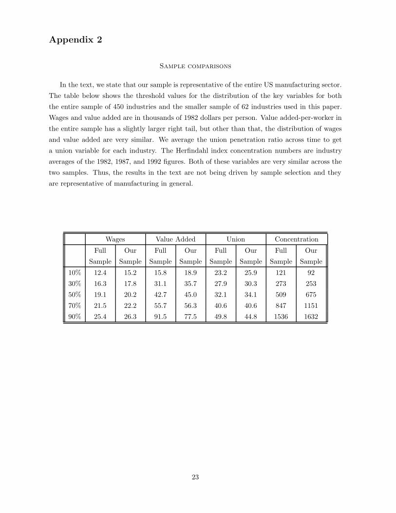
Sample comparisons

In the text, we state that our sample is representative of the entire US manufacturing sector.

The table below shows the threshold values for the distribution of the key variables for both

the entire sample of 450 industries and the smaller sample of 62 industries used in this paper.

Wages and value added are in thousands of 1982 dollars per person. Value added-per-worker in

the entire sample has a slightly larger right tail, but other than that, the distribution of wages

and value added are very similar. We average the union penetration ratio across time to get

a union variable for each industry. The Herfindahl index concentration numbers are industry

averages of the 1982, 1987, and 1992 figures. Both of these variables are very similar across the

two samples. Thus, the results in the text are not being driven by sample selection and they

are representative of manufacturing in general.

Wages Value Added Union Concentration

Full Our Full Our Full Our Full Our

Sample Sample Sample Sample Sample Sample Sample Sample

10% 12.4 15.2 15.8 18.9 23.2 25.9 121 92

30% 16.3 17.8 31.1 35.7 27.9 30.3 273 253

50% 19.1 20.2 42.7 45.0 32.1 34.1 509 675

70% 21.5 22.2 55.7 56.3 40.6 40.6 847 1151

90% 25.4 26.3 91.5 77.5 49.8 44.8 1536 1632

23

Appendix 3

Alternative wage construction

Because profitable industries may attract higher quality workers, we need to make sure that

any wage responsiveness to industry variables that we measure is not merely capturing the

higher wages that high-quality workers earn. To the extent that labor quality varies across

industry or time, our time and industry dummies will capture those movements. However, it

is possible that worker quality varies systematically across time and industry. Our database

cannot control for quality. Therefore, using data from the Current Population Survey from the

Bureau of Labor Statistics, we have constructed measures of the wages that workers could be

expected to earn based on their individual characteristics.

Building this “alternative wage” consists of three major steps. First using CPS data, we

predict the wage that each worker could expect to receive given his or her education, experience,

and other demographic characteristics. We then combine individual workers’ alternative wages

into an aggregate alternative wage for each industry. Next, we map those (Census) industries

into SIC codes so that we can match them up with our manufacturing data.

A.1 The CPS data and the basic regression

We use data from the CPS Outgoing Rotation Groups for 1979-1994.28 Our wage definition

is earnings per week, and our hourly wage definition is earnings per week divided by hours per

week. The log of each wage measure is regressed against the following variables:

• Education is grade attained or completed. Both the variable and its square are used.

• Age and its square are both included.

• Part time status is a dummy variable that is one if the person worked either part of the

time, all year, or part of the year.

• Marital status is a dummy that is one if the person is married–whether or not the spouse

is present.

• There are five race dummies. Some years have only three.

• Dummy variables for geographic location are included. For 1979-84, SMSA is the relevant

area. For 1986-94, MSA Fips is used.

• State dummies are included in 1985, when the location variables are missing.

• Two-digit occupation dummies are used.28We use outgoing rotation groups because the wage and hours series are more complete and consistent than

in the March tapes.

24

• Three-digit industry dummies are used for manufacturing. For non-manufacturing, 2-

digit industries are used.

• A gender dummy is included.

• Month dummies are included.

In order to calculate what each individual could make regardless of industry, we want to take

out the industry effects from the prediction. Therefore, the regression is run using all the

industry dummies, but the predicted wage is calculated by setting them equal to zero. We

exclude a constant from the regression and drop one dummy from each of the other sets. This

excluded group serves as a reference group. The alternative wage we predict can be thought

of as a premium over and above (or below) what the excluded group earns. Our reference

group is married, white, female, full-time schoolteachers who live in Washington, D.C. and were

interviewed in December. This group was chosen because these categories stayed identifiable

across all the years, despite changing variable definitions. We ran weighted regressions using

the final CPS weights.

A.2 Aggregating predicted wages

The predicted wages were then averaged within industries to obtain the alternative wage

estimate for workers in those industries.29 We did not use weighted averages because the weights

represent the weight in the population, not the industry. This procedure yields an alternative

wage measure for each Industry Classification Code for each year. The classification code is

from the 1970 Census for years 1979-82 and from the 1980 Census for 1983-94.

A.3 Matching Census industry definitions to SICs

The assignment of census industries to SIC codes is not straightforward. For the (CPS) years

of 1983-92, census codes are based on the 1980 census which uses the 1972 SIC codes. Since we

also use 1972 SIC codes, the mapping in the Appendix of the CPS documentation works fine.

One SIC industry, 334, straddles two census industries. Therefore, we assign a weighted average

of the alternative wages for those two census industries to SIC 334.

For the CPS years of 1971-82, census codes are based on the 1970 census which uses 1967

SIC codes. There are many changes between 1967 and 1972 so that the CPS mapping appendix

has to be altered according to the SIC revisions. There are also now many SIC codes that

straddle census industries. These straddlers belong to 18 census industry ‘groups’. We created

weighted averages of alternative wages for each group and assigned them to the ‘straddlers’.

Once alternative wages have been calculated for each (1972 based) SIC code for each year,

these are merged onto our basic dataset.29At this point, we also calculated some alternative wages for groups of industries. This facilitated the matching

of Census industry codes to SICs in the next section.

25

BIBLIOGRAPHY

Abowd, J. M., “The NBER Immigration, Trade, and Labor Markets Data Files”, NBER

Working Paper No.3351, 1990.

and H. S. Farber, “Product Market Competition, Union Organizing Activity, and

Employer Resistance”, NBER Working Paper No. 3353, 1990.

and T. Lemieux, “The Effects of Product Market Competition on Collective Bar-

gaining Agreements: The Case of Foreign Competition in Canada”, Quarterly Journal of

Economics, 108, p.983-1014, 1993.

Akerlof, G. and J. Yellen, “Fairness and Unemployment,” American Economic Review,

78 p.44-9, May, 1988.

Angrist, J. D. and A. B. Krueger, “Split Sample Instrumental Variables Estimates of the

Return to Schooling”, mimeo, NBER, September, 1994.

Blanchflower, D. G., A. J. Oswald and P. Sanfey, “Wages, Profit and Rent-Sharing”,

Quarterly Journal of Economics, 111, p.227-252, 1996.

Carruth, A. A. and A. J. Oswald, Pay Determination and Industrial Prosperity, Oxford

University Press, 1989.

Christofides, L. N. and A. J. Oswald, “Real Wage Determination and Rent-Sharing in

Collective Bargaining Agreements”, Quarterly Journal of Economics, 107, 985-1002, 1992.

Denny, K. and S. Machin, “The Role of Profitability and Industrial Wages in Firm-Level

Wage Determination”, Fiscal Studies, 12, 34-45, 1991.

Dickens, W. T. and L. F. Katz, “Inter-Industry Wage Differences and Industry Charac-

teristics”, in K. Lang and J. Leonard, Unemployment and the Structure of Labor Markets,

Basil Blackwell, 1987.

Estevao, M. M. and S. M. Tevlin, “The Role of Profits in Wage Determination: Evidence

from US Manufacturing”, FEDS Working Paper 95-48, November 1995.

Gardner, J. A., “An Analysis of the Employer and Employee Determinants of Pay Using

Matched Data”, mimeo, University of Warwick, 1999.

Gray, W., “Industry Productivity Database”, mimeo, Clark University, 1989.

Hildreth, A. K. G. and A. J. Oswald, “Rent-Sharing and Wages: Evidence from Company

and Establishment Panels”, mimeo, University of Essex and LSE, January, 1993.

26

Krueger, A. B. and L. H. Summers, “Reflections on the Inter-Industry Wage Structure”,

in K. Lang and J. Leonard, Unemployment and the Structure of Labor Markets, Basil

Blackwell, 1987.

Layard, R., S. Nickell, and R. Jackman, Unemployment: Macroeconomic Performance

and the Labour Market. Oxford; New York; Toronto and Melbourne: Oxford University

Press, 1991.

Lindbeck,A. and D. Snower, The Insider-Outsider Theory of Employment and Unemploy-

ment. Cambridge, MA and London: MIT Press, 1988.

, “Inter-Industry Wage Differentials and Incumbent Workers”, Working Paper, 1990.

McDonald, I. and R. Solow, “Wage Bargaining and Employment”, American Economic

Review, 71, 896-908, 1981.

Nickell, S. J. and P. Kong, “An Investigation into the Power of Insiders in Wage Deter-

mination”, Oxford Applied Economics Discussion Paper, No.49, 1988.

and S. Wadhwani, “Insider Forces and Wage Determination”, Economic Journal,

100, 496-509, 1990.

Salop, S.C., “A Model of the Natural Rate of Unemployment,” American Economic Review,

69 p.117. March, 1979.

Sanfey, P., “Wages and Insider-Outsider Models: Theory and Evidence for the US”, mimeo,

University of Kent, 1993.

Shapiro, C. and J.E. Stiglitz, “Equilibrium Unemployment as a Worker Discipline Device”,

American Economic Review, p.433-44, June, 1984.

Shea, J., “The Input-Output Approach to Instrument Selection”, Journal of Business and

Economic Statistics, 11, p.145-55, 1993.

Van Reenen, J., “The Creation and Capture of Rents: Wages and Innovation in a Panel of

U.K. Companies”, Quarterly Journal of Economics, 111, p.195-226, 1996.

27

Documents

Do Firms Share their Success with Workers? The Response of