1

DO EXPORTS CAUSE FIRM PRODUCTIVITY GROWTH? A MATCHING ANALYSIS FOR SMALL AND LARGE SPANISH

MANUFACTURING FIRMS*

Juan A. Máñez Castillejoa

María E, Rochina Barrachina

Juan A. Sanchis Llopis

Maja Barac

Universitat de València and LINEEX

Abstract

The trade literature has long discussed the existence of some benefits attributed

to exporting, among others, the improvement of firm productivity. This paper

examines whether firms starting to export enjoy better total factor productivity (TFP)

prospects than non-exporting firms. To examine this, we investigate if firms starting to

export perform better ex-ante (self-selection) than non-exporting firms and, conditional

on this fact, we analyze if they are also more productive ex-post (learning-by-

exporting). For this purpose, we use both non-parametric Kolmogorov-Smirnov tests

and matching techniques. The dataset is a sample of Spanish manufacturing firms

drawn from the Encuesta sobre Estrategias Empresariales for 1990-2002. Our results

shed light on the importance of considering differences in firm size when analyzing

both self-selection into exporting and post-entry productivity changes. They confirm

the existence of a process of self-selection into exporting for small firms, but not for

the large firms. However, we find evidence of post-entry productivity changes both for

large and small firms.

Key words: exports, total factor productivity, stochastic dominance, non-

parametric tests, matching techniques.

* We would like to thank the Instituto Valenciano de Investigaciones Económicas providing financial

support for this research and Fundación SEPI for providing the data. Usual disclaimers apply. a Corresponding author: Juan A. Máñez Castillejo, Universitat de València, Facultat d’Economia,

Departament d’Economia Aplicada II, Avda. dels Tarongers, s/n, 46022 València, Spain. jamc@uv.es

2

1. Introduction

In recent years, the literature analyzing the relationship between exports and

productivity using microdata has expanded to cover a wide range of different

countries.1 Some of the findings in this literature appear to be sensibly consistent:

exporters are generally larger and more productive than non-exporters, and there is

self-selection into export markets (i.e., only the ex-ante more efficient firms enter into

export markets).2 Melitz (2003) in a model with heterogeneous (productivity) firms that

have to incur sunk costs to entry in foreign markets formulates predictions that are

consistent with the above empirical findings.

In Melitz (2003) model a pool of heterogeneous potential export entrants that

operate in a monopolistically competitive industry have to incur sunk fixed cost to

export. However, each firm has to make a draw from an exogenous productivity

distribution which determines whether they produce and export. Further, an

endogenously determined productivity growth determines whether a firm exports or

not. Exporting increases expected profits, which stimulates entry, raises the survival

productivity threshold above the autarky one and drives out of the market the least

efficient firms. Three types of firms characterize the resulting productivity

distribution3: (i) exiters, firms with productivity higher than the autarky productivity

threshold but lower that the open economy domestic threshold; (ii) purely domestic

firms, those who operate in the domestic market but do not export, these firms have

1 For thorough reviews see Greenaway and Kneller (2007a) and Wagner (2007). 2 For previous results on self-selection see column 4 (pre-entry differences) in Table 3 of Greenaway and

Kneller (2007a) and column 3 (pre-entry differences) in Table A1 of Wagner (2007). 3 According to Melitz (2003) model there are three productivity thresholds determining if a firm produces

and exports: the autarky threshold which corresponds to the one domestic firms face to sell in the

domestic market when the country is not open to international markets; the open economy threshold that

corresponds to the threshold faced by domestic firms to sell in the domestic market for international

opened economies; and, the exporting threshold that is the one faced by firms to sell in the export

markets.

3

productivities higher than the open economy domestic threshold but lower than the

exporting one; and, (iii) exporters, firms with productivity higher than the export

threshold that combine domestic sales and exports. Further, whereas exporting allows

the most productive firms to expand, it forces less productive firms to contract.

Therefore, Melitz (2003) is consistent both with the evidence suggesting that exporting

firms are more productive than non-exporting ones and with self-selection into export

markets.

The empirical evidence on whether entry into export markets affects firm

performance (post-entry effects) is less compelling. This refers to the so-called

learning-by-exporting hypothesis, i.e. the possibility that having entered in the export

markets, firms become more productive. On theoretical grounds, the possible

productivity gains arise from growth in sales that allow firms to profit from economies

of scale, knowledge flows from international customers (that provide information about

process and product innovations reducing costs and improving quality) and from

increased competition in export markets that forces firms to behave more efficiently.

The first empirical works focused on the post-entry effects of exporting were made

within a framework of testing the hypothesis of self-selection versus learning-by-

exporting. These works failed to produce any convincing evidence on learning-by-

exporting.4 However, the growing international evidence in favour of the self-selection

hypothesis (following Bernard and Jensen, 1999) has substantially modified the

approach to test for post-entry effects of exporting.5 In this sense, recent studies

recognize that new exporters have many of the characteristics to become exporters (as 4 For example, Castellani (2002) for Italy, Baldwin and Gu (2003) for Canada, and Clerides et al. (1998)

for Colombia and Morocco, find evidence suggesting that productivity of exporting firms may increase

with export intensity. However, evidence in Delgado et al. (2002), for Spanish firms, is far from conclusive

(they only find supporting evidence for young firms). Finally, Bernard and Jensen (1999), Bernard and

Wagner (1997), Clerides et al. (1998) and Aw and Hawng (1995) do not find any evidence of learning-by-

exporting for the US, Germany, Colombia and Korea, respectively. 5 However, Hanson and Lundin (2004) and Greenaway et al. (2005) for Sweeden, and Damijan et al.

(2007) do not find evidence of self-selection.

4

compared to non-exporters) and consequently, selecting into exporting is not a

random process (only the higher productivity firms enter into the export markets).

Thus, if among non-exporters today those that will do it in the future are already

“better” than those that will not do it, one would find that these better firms would

perform better in the future even if they will not start exporting. Therefore, if selecting

into export is not a random process and firms either self-select or are selected

according to a certain criteria, the effect of exports on any firm performance dimension

cannot be simply evaluated by comparing the average performance of firms who start

to export and firms not exporting. In any case, either if the firm starts to export or not,

we do not have information about its performance in the counterfactual situation.

Matching techniques provide a way to construct a control group that provides each

firm starting to export a matched unit that is as similar as possible at the time before

the firm starts exporting. Differences between the two groups (the export starters and

the matched non-export starters) after starting to export can be attributed to the fact

that the former firms start to export (Heckman et al., 1999, provides a comprehensive

discussion in the evaluation of labour market programmes context).6

Table I shows that within the matching analysis evidence is also far from

conclusive. Whereas some works do not find any evidence of post-entry productivity

changes (see Wagner, 2002, and Arnold and Hussinger, 2005), those works that find

evidence differ in the span of the productivity changes produced by exporting. For the

UK, Greenaway and Kneller (2003), Greenaway and Kneller (2004) and Girma et al.

(2004) show that productivity growth in new exporters is faster than in non-exporters

one or at most two years after entry. Also for the UK, Greenaway and Kneller (2007b),

using different data, extend the period of extra productivity growth to three years, and

Hanson and Lundin (2004) obtain the same results for Sweden. Finally, De Loecker

6 Van Biesebroeck (2005) argues that not controlling for self-selection could lead to over-estimate the

effects of learning for new-exporters.

5

(2007) for Slovenia and Serti and Tomassi (2007) for Italy report evidence of a longer

period of extra-productivity growth (four and at least 6 years, respectively).

In this paper we investigate both if self-selection and post-entry firm

productivity changes differ across firm size using a sample of Spanish manufacturing.

If the productivity distribution is size dependent and large firms are more productive

than small ones, the exporting threshold identified by Melitz (2003), imposing self-

selection, could be binding for small but not for large firms. Analogously, if large firms

are highly productive before entering export markets the scope of productivity

improvements they could get by entering export markets might be smaller. Following

Delgado et al. (2002) we use stochastic dominance techniques to test for self-selection.

When testing for post-entry effects and to control for self-selection we use matching

techniques.

Our results shed light on the importance of considering differences in firm size

when analyzing self-selection into exporting and post-entry productivity changes.

Whilst, our results confirm the existence of a process of self-selection into exporting

for small firms, we do not find any evidence for their large counterparts. The joint

consideration of this evidence and the fact that pre-entry productivity is higher for

large firms suggests that the exporting threshold put forward by Melitz (2003) is

binding for small firms but not for large firms. However, we find evidence of post-entry

productivity changes both for large and small firms. For both size groups we detect

that the effect of exporting in productivity growth is not immediate, since for small

firms starts being significant one year after entry, and for large after two years.

The rest of the paper is organized as follows. Section 2 presents the data. Section 3

deals with total factor productivity measurement issues. Section 4 is devoted to the

analysis of the relationship between productivity and firm size. Section 5, 6 and 7

present the results on self-selection and post-entry productivity changes. Finally,

section 8 concludes.

6

2. Data.

The data used in this paper are drawn from the Encuesta sobre Estrategias

Empresariales (ESEE, hereafter) for the period 1990-2002.7 This is an annual survey

that is representative of Spanish manufacturing firms classified by industrial sectors

and size categories. It provides exhaustive information at the firm level.

The sampling procedure of the ESEE is the following. Firms with less than 10

employees were excluded from the survey. Firms with 10 to 200 employees were

randomly sampled, holding around 5% of the population in 1990. All firms with more

than 200 employees were requested to participate, obtaining a participation rate

around 70% in 1990. Important efforts have been made to minimise attrition and to

annually incorporate new firms with the same sampling criteria as in the base year, so

that the sample of firms remains representative of the Spanish manufacturing sector

over time.8

The panel nature of the dataset allows classifying firms according to their exporting

status over time. We select those firms that report information both on the exports

question and on all the variables involved in the construction of the productivity

measure. Applying this criterion we end up with a sample, corresponding to the period

1991-2002, made up of 18455 observations: 12685 observations for small firms (those

with 10 to 200 employees) and 5770 for large firms (those with more than 200

employees). In terms of firms we have 987 firms throughout the entire period, from

which 72.96% (1517) are small firms and 27.03% (562) are large firms.

Table II reports descriptive statistics of our sample on firm export activity, for

the period 1991-2002. The proportion of exporting firms steadily increased from

35.28% to 50.52% for small firms and from 84.41% to 94.14% for large firm, signalling

a trend of incorporation to the export market, especially of small firms. However, the

7 Although we do not use any observation for 1990 as we cannot compute TFP for this year. 8 See http://www.funep.es/esee/ing/i_esee.asp for further details.

7

export intensity (export to sales ratio) remained quite stable during the sample period,

being 24.03% and 32.51% (on average) for small firms and large firms, respectively.

3. Measurement of productivity.

To measure productivity we use a total factor productivity index (TFP, hereafter). This

is calculated at the firm level using a multilateral productivity index that is an

extension of the Caves et al. (1982) index, to account for the fact that firms with

different sizes are differently sampled in the data set. This extension was developed in

Good et al. (1996) and Delgado et al. (2002).

In order to calculate TFP we define the following dummy variables,

ττ⎧

= ⎨⎩

1 if firm belongs to size group 0 otherwise,f

fp

⎧= ⎨⎩

1 if firm belongs to industrial sector ( =1,...,18, NACE-CLIO R-25)0 otherwise.fs

f s sj

Having a sample of N firms (f=1,…,N) for T years (t=1,…,T),9 and assuming that

observations from different firms are independent, one can calculate the TFP index for

firm f belonging to size group τ and to industry s in year t, with the following

expression:

( ) ( )( ) ( )

=

=

= − − + − +

− − + −

∑

∑

Ii i i i

fs t fs t s fs t s fs t siI

i i i is s s s s s

i

y O O X X

O O X X

1

1

1ln ln ln ln2

1 ln ln ln ln ,2

τ τ τ τ τ τ τ

τ τ τ

ϖ ϖ

ϖ ϖ (1)

where fs tO τ is the output or production of firm f belonging to industry s with size τ in

year t, τϖ ifs t is the cost share of input i (i=1,...,I) and τ

ifs tX is the quantity of input i

used. The approach to calculate the series for capital, labour, other intermediate

inputs and output can be found in Delgado et al. (2002). Finally, we define

9 In practice, we will have Nt observations for each year, i.e. we will have an unbalanced panel of firms.

However, to keep the notation as simple as possible we do not show this explicitly in the formulae.

8

τ τ τ= =

= ∑∑1 1

1 N T

s fs t f fsf t

m m p jNT

and τ= =

= ∑∑1 1

1 N T

s fs t fsf t

m m jNT

, where τfs tm is alternatively

fs tOln τ , τϖ ifs t or τln i

fs tX .

The above index measures the TFP proportional difference of a firm f from industry

s and size τ in year t in relation with a reference firm. The reference firm varies

according to industry. For industry s, in particular, it is defined as the firm whose

outputs and inputs are equal to the geometric mean, across the sample period, of the

outputs and inputs of those firms that belong to industry s and, also, as the firm

whose input cost shares are equal to the arithmetic mean, during the sample period,

of the input cost shares of the firms belonging to industry s.

The first component of this index (the three first terms in expression 1), compares

the output and the use of inputs for each of the firms in period t with those of the

mean, across time, of firms belonging to the same industry and size group. This allows

for transitivity in the comparisons across firms belonging to the same size group. The

second component (three last terms in expression 1), preserves transitivity in the

comparison between firms belonging to the same industry but to different size groups.

This second term measures the difference between TFP of a mean firm from a

determined industry and size group, and TFP of an average firm (the average firm of all

belonging to the same industry, regardless its size). Finally, as we consider a different

reference firm across industries, we eliminate possible differences in TFP across

industries, which will also allow considering jointly firms belonging to different

industries.10

10 The way in which the TFP index is constructed allows pooling firms from different industries (according

to the NACE two digits classification) in the testing procedures.

9

4. On productivity and firm size.

In this section, we investigate whether the productivity distribution is size dependent,

i.e whether there are systematic differences in productivity between small and large

firms. Following the ESEE, we consider two groups of firms according to their size:

small firms are those with 10 to 200 employees, and large firms those firms with more

than 200 employees.

Figure I shows that the estimated TFP density for large firms is skewed towards

higher TFP levels than the corresponding for small firms, suggesting higher TFP levels

for large firms. Further, we compare, for each year, the TFP distributions of large and

small firms using stochastic dominance methods.

Figure II shows the relative distribution functions of TFP for large and small

firms, for each year of the period 1991-2002.11 These figures represent the equivalence

between each of the quantiles of the TFP distribution for large firms in the quantile

scale of the TFP distribution for small firms. The diagonal represents the uniform

distribution [0,1], i.e. the relative distribution if both distributions were identical. The

position of the relative distribution below the diagonal suggests that the distribution

represented in the vertical axis stochastically dominates the distribution in the

horizontal axis. In the figure we can see that the relative TFP distributions are below

the diagonal for all years analysed, suggesting that the TFP distribution for large firms

stochastically dominates that for small firms in each period t.

Given the observed differences, the next step is to formally test if the TFP

distribution of large firms in t stochastically dominates the TFP distribution of small

firms in t. Thus, for each time period, we compare

( ) ( ) =t t t tF y vs. G y t, 1991,...,2002 (2)

11 See Handcock and Morris (1999) for the technical details about relative distributions.

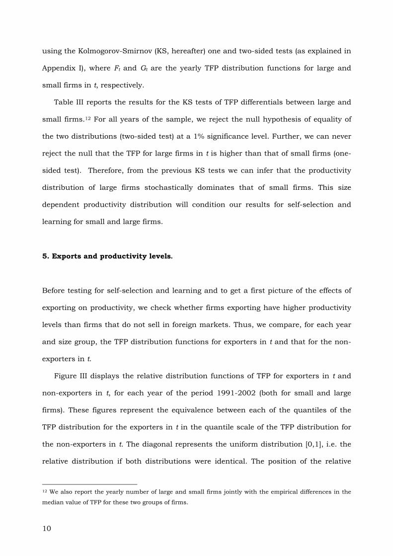
10

using the Kolmogorov-Smirnov (KS, hereafter) one and two-sided tests (as explained in

Appendix I), where Ft and Gt are the yearly TFP distribution functions for large and

small firms in t, respectively.

Table III reports the results for the KS tests of TFP differentials between large and

small firms.12 For all years of the sample, we reject the null hypothesis of equality of

the two distributions (two-sided test) at a 1% significance level. Further, we can never

reject the null that the TFP for large firms in t is higher than that of small firms (one-

sided test). Therefore, from the previous KS tests we can infer that the productivity

distribution of large firms stochastically dominates that of small firms. This size

dependent productivity distribution will condition our results for self-selection and

learning for small and large firms.

5. Exports and productivity levels.

Before testing for self-selection and learning and to get a first picture of the effects of

exporting on productivity, we check whether firms exporting have higher productivity

levels than firms that do not sell in foreign markets. Thus, we compare, for each year

and size group, the TFP distribution functions for exporters in t and that for the non-

exporters in t.

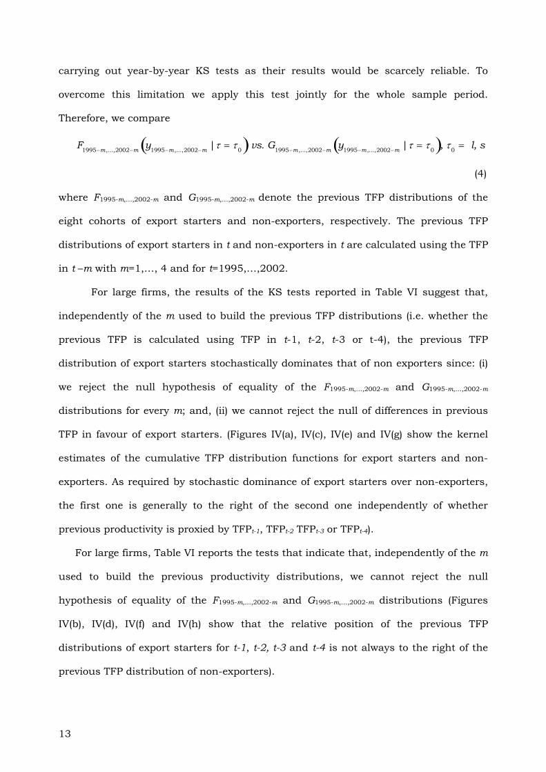
Figure III displays the relative distribution functions of TFP for exporters in t and

non-exporters in t, for each year of the period 1991-2002 (both for small and large

firms). These figures represent the equivalence between each of the quantiles of the

TFP distribution for the exporters in t in the quantile scale of the TFP distribution for

the non-exporters in t. The diagonal represents the uniform distribution [0,1], i.e. the

relative distribution if both distributions were identical. The position of the relative

12 We also report the yearly number of large and small firms jointly with the empirical differences in the

median value of TFP for these two groups of firms.

11

distribution below the diagonal suggests that the distribution represented in the

vertical axis stochastically dominates the distribution in the horizontal axis.

In the figure we can see that for small firms the relative TFP distributions are below

the diagonal for all years analysed (except for 1999 and 2002, for which the

distributions are partly above the diagonal), suggesting that the TFP distribution for

exporters in t stochastically dominates that for the non-exporters in t. For large firms,

the results are not so clearly defined as the relative distribution functions for a

majority of the years lie (totally or partially) above the diagonal. Therefore, for large

firms we can not conclude that the TFP distribution for exporters in t stochastically

dominates that for the non-exporters in t. On the basis of the observed differences in

the figures, we formally test whether the TFP distribution of exporters in t

stochastically dominates the TFP distribution of non-exporters in t. Thus, for each

time period and size group, we compare

Ft yt |τ = τ0( ) vs. Gt yt |τ = τ0( ), t = 1991,...,2002; τ0 = l(large), s(small) (3)

using the KS one and two-sided tests, where Ft and Gt are the yearly TFP distribution

functions for exporters and non-exporters in t, respectively.

Table IV shows the results for the KS tests for TFP differentials.13 For small firms,

we reject the null hypothesis of equality of the two distributions (at a 5% significance

level) for all years, except for 1991 and 2002. Further, we can never reject the null

that the TFP of exporters in t is higher than that of non-exporters. For large firms, we

only reject the null hypothesis of equality of the TFP distributions four years of the

sampling period (1994, 1995, 1997 and 1998). For these years we can not reject the

null that the TFP for exporters in t is higher than that for non-exporters.

Thus, we can draw two conclusions from the previous KS tests: (i) the TFP

distribution for small firms that export stochastically dominates that of non-exporters

13 We also report the yearly number of exporters and non-exporters jointly with the empirical differences

in the median value of TFP for these two groups of firms.

12

almost except for two years out of twelve (1991 and 2002); and, (ii) for large firms the

above conclusion only holds for four years of the sampling period (1994, 1995, 1997

and 1998).

6. Do firms self-select into exports?

According to self-selection, only the more efficient firms self select into exporting. To

provide empirical evidence on self-selection into exporting, we compare TFP previous

to start exporting of export starters and non-exporters. Export starters in t are firms

that did not exported for four years prior to year t and export in t; and non-exporters

in t are firms that neither exported for four years prior to period t nor in t. As our

sample covers the period 1991 to 2002 we can construct 8 cohorts of export starters

in t, from 1995 to 2002. The choice of four previous years without exporting to

consider a firm that export in t as an export starter in t is a compromise between the

willingness to ensure that the export starter TFP is not affected for previous exporting

experience, and the need of working with a reasonable number of exports starter to

carry out the analysis.14

To compare the previous TFP levels (TFPt-m) of export starters in t and non-

exporters in t we follow a sequential approach: first, we test, using KS tests, whether

the previous TFP of export starters in t stochastically dominates that of non-exporters

in t; and, second we use regression techniques to quantify the advantages in previous

TFP of export starters in t over non-exporters in t .

To carry out the first stage, we should compare for every t (for t = 1995,…, 2002),

the previous TFP distributions for export starters in t with that of non-exporters in t

using KS tests. However, the small size of the cohorts of exports starters between 1995

y 2002 (in table V we report the number of export starters each year) suggests not

14 Imposing larger periods without exporting reduces drastically the number of export starters.

13

carrying out year-by-year KS tests as their results would be scarcely reliable. To

overcome this limitation we apply this test jointly for the whole sample period.

Therefore, we compare

F1995−m,...,2002−m y1995−m,...,2002−m |τ = τ0( ) vs. G1995−m,...,2002−m y1995−m,...,2002−m |τ = τ0( ), τ0 = l, s

(4)

where F1995-m,…,2002-m and G1995-m,…,2002-m denote the previous TFP distributions of the

eight cohorts of export starters and non-exporters, respectively. The previous TFP

distributions of export starters in t and non-exporters in t are calculated using the TFP

in t –m with m=1,…, 4 and for t=1995,…,2002.

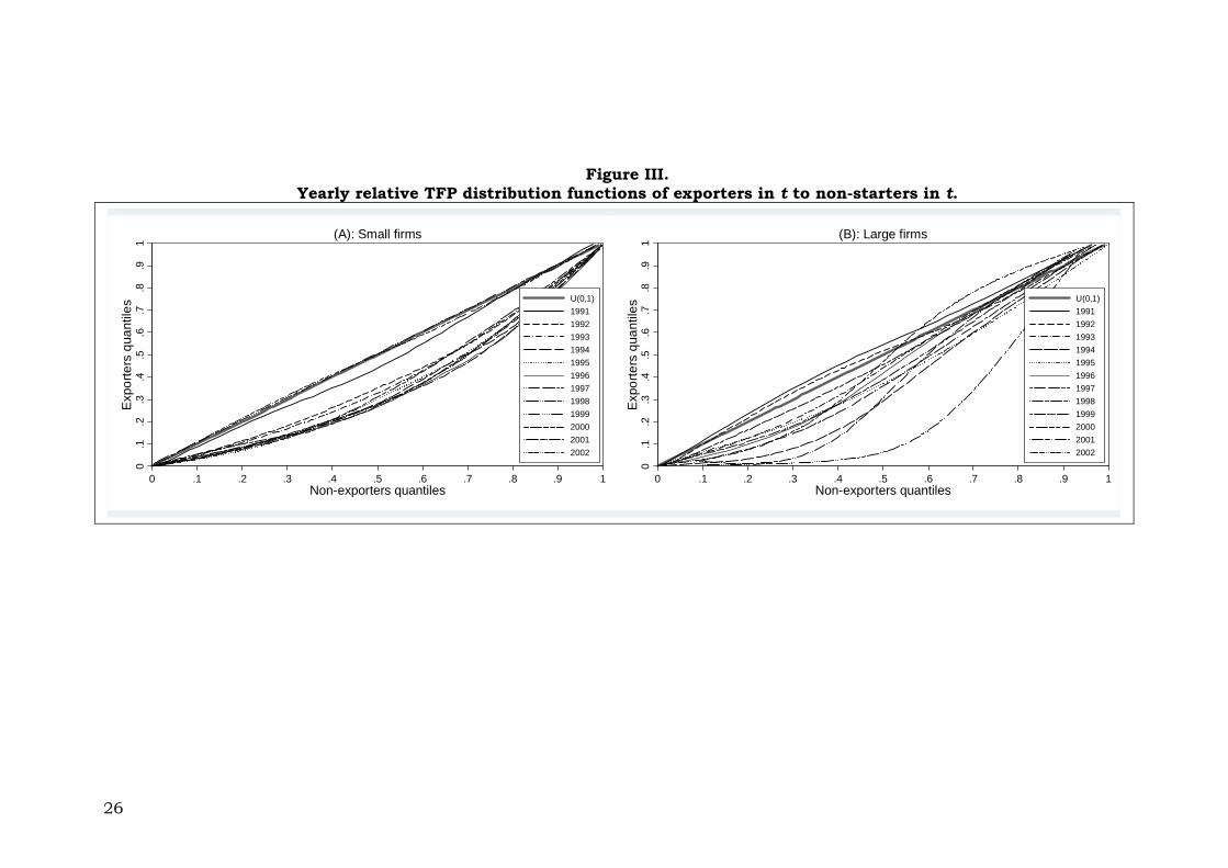
For large firms, the results of the KS tests reported in Table VI suggest that,

independently of the m used to build the previous TFP distributions (i.e. whether the

previous TFP is calculated using TFP in t-1, t-2, t-3 or t-4), the previous TFP

distribution of export starters stochastically dominates that of non exporters since: (i)

we reject the null hypothesis of equality of the F1995-m,…,2002-m and G1995-m,…,2002-m

distributions for every m; and, (ii) we cannot reject the null of differences in previous

TFP in favour of export starters. (Figures IV(a), IV(c), IV(e) and IV(g) show the kernel

estimates of the cumulative TFP distribution functions for export starters and non-

exporters. As required by stochastic dominance of export starters over non-exporters,

the first one is generally to the right of the second one independently of whether

previous productivity is proxied by TFPt-1, TFPt-2 TFPt-3 or TFPt-4).

For large firms, Table VI reports the tests that indicate that, independently of the m

used to build the previous productivity distributions, we cannot reject the null

hypothesis of equality of the F1995-m,…,2002-m and G1995-m,…,2002-m distributions (Figures

IV(b), IV(d), IV(f) and IV(h) show that the relative position of the previous TFP

distributions of export starters for t-1, t-2, t-3 and t-4 is not always to the right of the

previous TFP distribution of non-exporters).

14

After detecting differences in previous productivity in favour of export starters

(as compared with non-exporters) for small firms but not for large firm, we proceed to

quantify the extent of these productivity differentials estimating the following reduced

form equation:

β β β β β ε− = + + + + +i t m L S L S i iy D D D D X, 0 1 2 3 4 (5)

where yi,t-m is the TFP for firm i in period t-m (for m=1,.., 4) of the cohort of export

starters and non-exporters in t (for t=1995,…,2002). DL is a dummy variable that takes

the value one for large firms, and DS is a dummy variable that takes the value one for

export starters (as opposed to non-exporters). Xi is a vector of control variables that

includes the log of firm age and its square.

By construction, β0 is the average previous TFP of small non-exporters, and

β0+β1 the average previous TFP of large non-exporters. β2 and β2+β3 are the average

export premia for small firms and large firms, respectively (export premium is defined

as the differential in previous TFP between export starters and non-exporters).

Further, β1 and β1+β3 are the average differentials in previous TFP between large and

small non-exporters, and large and small export starters, respectively.

To facilitate the interpretation of our results, the estimated coefficients (or

combination of coefficients), measuring average export premia and previous TFP

differentials between small and large firms, have been transformed to be interpreted as

percentages.15 These transformed coefficients are shown in Table VII and indicate that:

(i) export premium for small firms is within a 5.2% to 6.6% range (depending on

whether previous TFP is calculated with TFP in t-1, t-2, t-3 or t-4); and, (ii) for large

firms there is no difference between the previous TFP of export starters and non-

exporters. Further, our estimates show that previous TFP of large firms (either export

15 The estimated coefficient β̂ have been transformed by ( )( )β −ˆ100 exp 1 .

15

starters or non-exporters) is about 50% higher than that of small firms, confirming the

already noted relationship between productivity and size.

Hence, our results confirm the existence of a process of self-selection into export

markets for small firms but not for large firms. These results can be interpreted within

Melitz (2003) framework that allows for within industry heterogeneous productivity of

firms. The exporting threshold as defined by Melitz (2003) could be acting as a self-

selection mechanism for small firms but not for large firms. Previous productivity

levels of most large firms could be above of the common exporting threshold for large

and small firms, and the exporting threshold could be not binding for large firms.

7. Post-entry productivity growth: does export entry boost productivity growth?

Once we have empirically confirmed that there is a process of self-selection into

exporting, the next step is to check if exporting improves firm productivity. In the

absence of any information about the counterfactual situation for export starters

(what would have happened to export starters if they had not started to export), a first

stream in the literature has been to use as control group all the remaining firms

(Bernard and Jensen, 1995 or Delgado et al., 2002). However, the fact that the best

firms self-select to entry into export markets provides evidence that the sample of

firms starting to export is not a random sample. Thus, the simple comparison of the

TFP growth of export starters and non-exporters, after the former start to export, does

not allow to actually asses if the observed differences are due to learning-by-exporting

or to self-selection.

In order to control for the non-random nature of selection to enter into export

markets, a second stream of the literature (see Table I for a compendium of the most

relevant works) uses matching techniques to select a control group, from the pool of

non-exporters, to be compared with the exports starters, in which the distribution of

16

observed variables in the pre-entry period is as similar as possible to the distribution

in the starter group.

More formally, let ∆y denote the growth rate of TFP and Dit ∈ {0, 1} be an

indicator of whether firm i is an export starter in period t (as opposed to non-exporter

in t as defined in the former section). Thus, we can use +∆ 1it sy to define the TFP growth

between t and t+s, s≥0, for firm i classified as export starter in t, and +∆ 0it sy as the

outcome for firm i if it had not started to export. Thus, the causal effect of exporting

for firm i at time period t+s can be defined as

+ +∆ − ∆1 0it s it sy y (6)

Following the evaluation literature (see Heckman et al., 1997), we can define the

average effect of exporting on firms who start to export as

( )( ) ( ) ( )+ + + +∆ − ∆ = = ∆ = − ∆ =it s it s it it s it it s itE y y D E y D E y D1 0 1 01 1 1 (7)

The main problem of causal inference is that in observational studies the

counterfactual +∆ 0it sy is not observed, and therefore it has to be generated. Thus,

causal inference relies on the construction of the counterfactual for this term, which is

the average productivity growth that export starters would have experienced had they

not started to export. We overcome this problem using matching techniques to identify

among the pool of non-exporters in t those with a distribution of observable variables

affecting productivity growth and the probability of exporting as similar as possible to

that of export starters in t. It is then assumed that, conditional on X, firms with the

same characteristics are randomly exposed to the export activities, i.e. conditional on

X the potential productivity growth of export starters is independent of their export

status. Thus, (7) can be rewritten as

( ) ( )+ +∆ = − ∆ =it s it it it s it itE y X D E y X D1 0, 1 , 0 (8)

17

Since the set of observable variables that can potentially affect firms probability of

exporting and their productivity growth is quite large a problem that is needed to deal

with is the choice of the appropriate variable to match firms, or in case of using more

than one variable the appropriate weights. We solve this problem using the propensity

score techniques proposed by Rosenbaum and Robin (1983). Adapted to exports, it can

be shown that if starting to export is random conditioning upon X, it is also random

conditioning on the probability of exporting that they call propensity score.

Therefore, before performing the matching itself we obtain the probability of

becoming an export starter (propensity score) as the predicted probability of the

following probit model

−= =it it itP D F X D1( 1) ( , ) (9)

where Dit is a set of industry and time dummies. The set of observable characteristics

included in Xit is detailed in Table AII.1 of Appendix II.16

In order to construct the counterfactual we have chosen kernel matching. This

method matches all the export starters with a weighted average of some (all) non-

exporters with weights inversely proportional to the distance between the propensity

score of export starters and non-exporters (Becker and Ichino, 2002).17 Matching is

performed using the psmatch2 command (Leuven and Sianesi, 2003).

Following the matching analysis, we compare the productivity growth export

starters and matched non-exporters for the period t-1 to t+4 and for the sub-periods t-

16 In estimating the propensity score we include in the probit model the following relevant variables: the

interactions of TPF in t-1 and a dummy variable for large firms and a dummy variable for small firms; log

of size and log of size squared, both in t-1; industry dummies in t-1; log of age and log of age squared,

both in t-1; a variable capturing the technological effort ratio of the firm in t-1; the proportion of qualified

workforce of the firm in t-1; a dummy variable accounting if the firm does any complementary R&D

activity, in t-1; firm advertising intensity in t-1; a dummy variable accounting for the fact that the firm

capital is participated in more than a 25% by a foreign firm, in t-1; industry dummies in t-1; and, time

dummies. 17 We use the Epanechnikov kernel since it is the more common when applying matching techniques.

Notwithstanding, to show the robustness of our results we show in Appendix III the results using

Gaussian and Biweight kernel instead (see Table A.III.1)

18

1/t, t-1/t+1, t-1/t+2 and t-1/t+3. Table VIII reports the results of these comparisons,

both for small and for large firms.18 For the whole period (t-1 to t+4), it is true that,

both for small and large firms, TFP growth is higher for export starters than for non-

starters. Furthermore, the productivity growth advantage is higher for large export

starters than for small export starters: 10.7% and 16.5%, respectively. This time span

of extra-productivity growth for starters seems to be in line with De Loecker (2007)

for Slovenia, Hanson and Lundin (2004) for Sweeden, Serti and Tomassi (2007) for

Italy. Further, Greenaway and Kneller (2007b) for the UK that provide evidence

supporting a period of extra-productivity growth not shorter than three years.

However, Greenaway and Kneller (2003, 2004) and Girma et al. (2004) for the UK

found that the period of extra productivity growth lasted just one year. It is also

important to note that our estimated extra-productivity growth is substantially higher

than that obtained in most papers using matching techniques (see Table I), although

similar to the 17% obtained by Tomassi and Serti (2007) for the case of Italy.

The analysis per sub-period also raises two interesting points. First, differently

from results for other countries, neither for small firms nor for large firms the extra

productivity growth start the year of entry in the export market. For small firms, it is

only from the sub-period t-1/t+1 that we detect that the productivity growth of export

starters is higher than that of non-exporters. For large firms, the length of the period

needed to detect extra-productivity growth is even longer since it starts in sub-period

t-1/t+2 (in this subperiod the productivity growth of export starters is significantly

higher than that of non-exporters at 10% level). Second, for large firms the extra

productivity growth increases with the time elapsed from entry in export markets,

18 Due to the fact that we have previously estimated the propensity scores, p-values are calculated

through bootstrapping techniques with 1000 replications.

19

suggesting the existence of a process of increasing returns to exporting. For small

firms we do not find such evidence.19

8. Concluding remarks.

This paper has examined both the self-selection into export markets and the post-

entry productivity changes explicitly considering the impact of firm size. Our main

empirical results may be summarised as follows. First, whereas we find evidence in

favor of the existence of a process of self-selection into exporting for small firms, we do

not find any evidence for their large counterparts. The joint consideration of this

evidence and the fact that pre-entry productivity is higher for large firms suggests that

the exporting threshold put forward by Melitz (2003) is binding for small firms but not

for large firms.

Second, we find evidence of post-entry productivity changes both for large and

small firms. Differently from previous research, we detect for both size groups that the

effect of exporting on productivity growth is not immediate, since for small firms starts

being significant one year after entry, and for large after two years. Further, we find

that for large firms the extent of the extra productivity growth increases along the time

since entry in export markets, suggesting the existence of increasing returns to

exporting. For small firms we do not find such evidence.

Our analysis clearly suggests that export subsidising in not the right policy

alternative. Since, especially for small firms, productivity seems a barrier to enter into

export markets, policies addressed to increase export participation should include

measures aimed to increase firm productivity such as easing the access to new

production technologies and qualified labour force. Further, as the beneficial effects of

exporting on productivity only materialize some time after entry, there is a need of 19 One should be cautious about some of the results obtained for large firms due to the small sample of

firms used.

20

policies addressed to ease the permanence of firms in foreign markets once they start

exporting.

21

REFERENCES.

Arnold, J. and K. Hussinger, 2005, “Exports versus FDI in German manufacturing:

firm performance and participation in international markets”, mimeo, World

Bank.

Aw, B.Y. and A. Hwang, 1995, “Productivity and the export market: A firm-level

analysis”, The World Bank Economic Review, 14, 1-65.

Baldwin, J.R. and W. Gu, 2004, “Trade liberalisation: export-market participation,

productivity growth and innovation”, Oxford Review of Economic Policy, 20,

372–92.

Becker, S. and A. Ichino, 2002, “Estimation of average treatment effects based on

propensity scores”, Stata Journal, 2, 358-377.

Bernard, A.B. and J.B. Jensen, 1995, “Exporters, jobs, and wages in US

manufacturing: 1976-1987”, Brookings papers on economic activity:

microeconomics, 67-112.

Bernard, A.B. and J.B. Jensen, 1999, “Exceptional exporter performance: cause,

effect, or both”, Journal of International Economics, 47, 1-25.

Bernard, A. and J. Wagner, 1997, “Exports and success in German manufacturing”,

Review of World Economics/Weltwirtschaftliches Archiv, 133, 134–57.

Castellani, D., 2002, “Export behaviour and productivity growth: evidence from Italian

manufacturing firms”, Weltwirtschaftliches Archiv, 138, 605-628.

Caves, D.W., L.R. Christensen and E. Diewert, 1982, ‘Multilateral comparisons of

output, input and productivity using superlative index numbers’, Economic

Journal 92, 73-86.

22

Clerides, S.K., S. Lach, and J.R. Tybout, 1998, “Is learning by exporting important?

Micro-dynamic evidence from Colombia, Mexico, and Morocco,” Quarterly

Journal of Economics, 113, 903-948.

Damijan, J., S. Polanec, J. and Prašnikar, 2007, “Self-selection, export market

heterogeneity and productivity improvements: firm level evidence from

Slovenia”, The World Economy, 30, 135–55.

De Loecker, J., 2007, “Do exports generate higher productivity? Evidence from

Slovenia”, Journal of International Economics, 73, 69-98.

Delgado, M.J., J.C. Fariñas, and S. Ruano, 2002, “Firms’ productivity and the export

markets,” Journal of International Economics, 57, 397-422.

Good, D., I.M. Nadiri and R. Sickles, 1996, ‘Index number and factor demand

approaches to the estimation of productivity’, NBER working paper 5790.

Girma, S., D. Greenaway, and R. Kneller, 2004, “Entry to export markets and

productivity: a microeconomic analysis of matched firms”, Review of

International Economics, 12, 855-866.

Greenaway, D., J. Gullstrand, and R. Kneller, 2005, “Exporting may not always boost

firm level productivity”, Weltwirtschaftliches Archiv, 141, 561–82.

Greenaway, D., and R. Kneller, 2003, “Exporting, productivity and agglomeration: a

matched difference in difference analysis of matched firms”, GEP Research

Paper 03/45, Leverhulme Centre for Research on Globalisation and Economic

Policy, University of Nottingham.

Greenaway, D., and R. Kneller, 2004, “Exporting and Productivity in the UK”, Oxford

Review of Economic Policy, 20, 429-439.

Greenaway, D and R. Kneller, 2007a, “Firm heterogeneity, exporting and foreign direct

investment”, The Economic Journal, 117, 134-161.

23

Greenaway, D and R. Kneller, 2007b, “Industry Differences in the Effect of Export

Market Entry: Learning by Exporting?”, Review of World Economics, 143, 416-

432.

Handcock, M.S. and M. Morris, 1999, “Relative distribution methods in the social

sciences”, New York: Springer-Verlag.

Hansson, P. and N. Lundin, 2004, “Exports as indicator on or a promoter of successful

Swedish manufacturing firms in the 1990s”, Weltwirtschaftliches Archiv, 140,

415–45.

Heckman, J., R.J. Lalonde and J.A. Smith, 1999, “The economics and econometrics of

active labour market programs”, in O.C. Ashenfelter and D. Card (Eds.).

Handbook of Labour Economics, vol 3A. North Holland, Amsterdam.

Heckman, J., H. Ichimura and P. Todd, 1997, “Matching as an econometric evaluation

estimator”, Review of Economic Studies, 65, 261-294.

Kolmogorov, A. N., 1933: “Sulla determinazione empirica di une legge di

distribuzione”, Giornale dell Istituto Italiano degli Attuari, 4, 83-91.

Leuven, E, and B. Sianesi, 2003. “PSMATCH2: Stata module to perform full

Mahalanobis and propensity score matching, common support graphing, and

covariate imbalance testing”, Statistical Software Components S432001, Boston

College Department of Economics, revised 28 Dec 2006.

Levinsohn, J. and A. Petrin, 2003, “Estimating production functions using inputs to

control for unobservables”, Review of Economic Studies, 70, 317-342.

Melitz, M.J., 2003, “The impact of trade in intra-industry reallocations and aggregate

industry productivity”, Econometrica, 71, 1695-1725.

Rosenbaum, P.R. and D. Rubin, 1983, “The central role of the propensity score in

observational studies for causal effects”, Biometrika, 70, 41-55.

24

Serti, F. and C. Tomasi, 2007, “Self-selection and post-entry effects of exports.

Evidence from Italian manufacturing firms”, Sant´ Anna School of Advanced

Studies, mimeo.

Smirnov, N. V., 1939: “On the estimation of the discrepancy between empirical curves

of distribution for two independent samples”, Bull. Math. University of Moscow,

2, 3-14.

Van Biesebroeck, J., 2005 “Exporting raises productivity in Sub-Saharan

manufacturing plants”, Journal of International Economics, 67, 373–91.

Wagner, J., 2002, “The causal effects of export on firm size and labour productivity:

first evidence from a matching approach”, Economics Letters, 77, 287-292.

Wagner, J., 2007, “Exports and productivity: a survey of the evidence from firm level

data”, The World Economy, 30, 60-82.

25

Figure I. TFP density functions of large firms to small firms.

0.5

11.

52

dens

ity

-6 -4 -2 0 2TFP

Large Firms Small firms

Figure II. Yearly relative TFP distribution functions of large firms to small firms.

0.1

.2.3

.4.5

.6.7

.8.9

1La

rge

firm

s qu

antil

es

0 .1 .2 .3 .4 .5 .6 .7 .8 .9 1Small firms quantiles

U(0,1)199119921993199419951996199719981999200020012002

26

Figure III. Yearly relative TFP distribution functions of exporters in t to non-starters in t.

0.1

.2.3

.4.5

.6.7

.8.9

1E

xpor

ters

qua

ntile

s

0 .1 .2 .3 .4 .5 .6 .7 .8 .9 1Non-exporters quantiles

U(0,1)199119921993199419951996199719981999200020012002

(A): Small firms

0.1

.2.3

.4.5

.6.7

.8.9

1E

xpor

ters

qua

ntile

s

0 .1 .2 .3 .4 .5 .6 .7 .8 .9 1Non-exporters quantiles

U(0,1)199119921993199419951996199719981999200020012002

(B): Large firms

27

Figure IV. Comparing previous TFP levels of export starters and non-exporters.

0.2

5.5

.75

1C

umul

ative

prob

abilit

y

-2 -1 0 1Productivity

Non exporters Export starters

(a): Small firms (TFP in t-1)

0.2

5.5

.75

1C

umul

ative

prob

abilit

y

-1 0 1Productivity

Non exporters Export starters

(b): Large firms (TFP in t-1)

0.2

5.5

.75

1C

umul

ativ

e pr

obab

ility

-2 -1 0 1Productivity

Non exporters Export starters

(c): Small firms (TFP in t-2)

0.2

5.5

.75

1C

umul

ative

prob

ability

-1 0 1Productivity

Non exporters Export starters

(d): Large firms (TFP in t-2)

0.2

5.5

.75

1C

umul

ativ

e pr

obab

ility

-2 -1 0 1Productivity

Non exporters Export starters

(e): Small firms (TFP in t-3)

0.2

5.5

.75

1C

umul

ativ

e pr

obab

ility

-1 0 1Productivity

Non exporters Export starters

(f): Large firms (TFP in t-3)

0.2

5.5

.75

1C

umul

ativ

e pr

obab

ility

-2 -1 0 1Productivity

Non exporters Export starters

(g): Small firms (TFP in t-4)

0.2

5.5

.75

1C

umul

ativ

e pr

obab

ility

-1 0 1Productivity

Non exporters Export starters

(h): Large firms (TFP in t-4)

28

Table I: Main results on post-entry productivity changes using matching techniques. Country Sample Productivity measure Matching method Results

Wagner (2002) Germany 10425 firms 1978-1989

Labour productivity (average sales per person)

Nearest-neighbour No evidence of a casual relationship from exporting to productivity growth

Arnold and Hussinger (2005) Germany 389 firms 1992-2000

TFP as residual from a Cobb-Douglas production function

One-to-one nearest-neighbour No evidence of higher productivity growth for exporters

Greenaway and Kneller (2003) UK 11225 firms 1989-2002

TFP as residuals from a production function

Nearest-neighbour Entry to export markets is associated with a significant increase in TFP (ranking from 2.7 to 5.5% in TFP and 2.7 in labour productivity). There is no robust evidence of extra-productivity growth after two years from entry.

Greenaway an Kneller (2004) UK 11225 firms 1989-2002

TFP as residuals from a production function Labour productivity

Nearest neighbour Differences in extra-productivity growth between export entrants and non-exporters are significant only the year of entry in export markets (extra productivity growth 3.6%)

Girma, Greenaway and Kneller (2004)

UK 8992 firms 1988-1999

TFP as residual from a Cobb-Douglas production function

Nearest-neighbour On the entry year, export starters experience a TFP growth rate 1.6% higher than non starters. TFP continues to grow by an extra percentage point in the following year.

Greenaway and Kneller (2007b) UK 12875 observations 1990-1998

TFP as residuals of an econometrically estimated production function

Nearest-neighbour After controlling for industry effects, Significant effect on TFP growth of firms following export market entry: on average, TFP growth of new exporters is 2.9% faster than that of non exporters for in each of the three years following entry.

Serti and Tomassi (2007) Italy 38771 firms 1989-1997

TFP (following Levinsohn and Petrin, 2003 semi-prametric technique) Labour productivity

Kernel matching (Epanenchnikov Kernel)

The effect of exports on productivity growth is immediate and enlarges after some years following the entry period (after one year exporting 2% after six years 17%)

De Loecker (2007) Slovenia 6391 firms 1994-2000

TFP (own modification of Levinsohn and Petrin, 2003)

Nearest-neighbour Exporters experience higher productivity growth than non-exporters. Productivity growth of starters is 12.4% higher after four years exporting.

Hanson and Lundin (2004) Sweden 3275 firms 1990-1999

Total Factor Productivity Index

Nearest-neighbour Exports starters productivity growth is on average 2.2% higher than that of non-exporters for three years after the entry.

29

Table II. Number of exporters and export intensity. 1991 1992 1993 1994 1995 1996 1997 1998 1999 2000 2001 2002 Total 1. Small firms Number of Exporters 272 349 385 413 431 475 594 582 584 593 541 539 5758 Number of Non-exporters 499 614 669 614 548 566 640 564 589 572 524 528 6927 % of Exporters 35.28% 36.24% 36.53% 40.21% 44.02% 45.63% 48.14% 50.79% 49.79% 50.90% 50.80% 50.52% 44.90% Export/Sales for exporters (%) 20.28% 20.92% 22.29% 24.51% 23.80% 23.53% 25.16% 25.09% 24.47% 25.02% 24.94% 24.94% 24.03% Export/Sales (%) 7.16% 7.58% 8.14% 9.86% 10.48% 10.74% 12.11% 12.73% 12.18% 12.74% 12.49% 12.60% 10.73% 2. Large firms Number of Exporters 341 412 432 481 450 429 444 422 423 518 446 434 5232 Number of Non-exporters 63 63 58 69 54 52 37 30 23 33 29 27 538 Export/Sales for exporters (%) 23.10% 24.60% 27.77% 29.65% 31.38% 32.56% 34.71% 35.67% 36.39% 36.84% 36.61% 37.55% 32.51% % of Exporters 84.41% 86.74% 88.16% 87.45% 89.29% 89.19% 92.31% 93.36% 94.84% 94.01% 93.89% 94.14% 90.65% Export/Sales (%) 19.50% 21.33% 24.48% 25.93% 28.40% 29.04% 32.04% 33.30% 34.51% 34.64% 34.38% 35.35% 29.41%

Table III. Yearly TFP differences between large and small firms.

Number of observations Equality of distributions Differences favourable to exporters

Year Large Small

TFP

differencesa Statistic p-value Statistic p-value

1991 407 773 0.300 7.191 0.000 0.000 1.000 1992 476 963 0.402 10.582 0.000 0.000 1.000 1993 493 1054 0.419 11.504 0.000 0.112 0.975 1994 553 1028 0.428 12.502 0.000 0.013 1.000 1995 508 984 0.420 11.932 0.000 0.000 1.000 1996 482 1041 0.426 12.617 0.000 0.000 1.000 1997 485 1236 0.453 13.915 0.000 0.000 1.000 1998 453 1146 0.448 13.829 0.000 0.000 1.000 1999 448 1175 0.440 13.792 0.000 0.000 1.000 2000 554 1165 0.461 15.269 0.000 0.000 1.000 2001 478 1067 0.450 14.344 0.000 0.000 1.000 2002 462 1067 0.340 10.231 0.000 0.005 1.000

a TFP differences (between both groups of firms) are calculated at the median of the distributions.

30

Table IV. Yearly TFP differences between exporters in t and non-exporters in t. Number of observations Equality of distributions Differences favourable to exporters

Year Exporters Non-exporters

TFP

differencesa Statistic p-value Statistic p-value

Small firms 1991 272 499 0.046 11.676 0.112 0.275 0.860 1992 349 614 0.076 2.324 0.000 0.049 0.995 1993 385 669 0.099 2.754 0.000 0.030 0.998 1994 413 614 0.109 3.567 0.000 0.001 1.000 1995 431 548 0.102 3.510 0.000 0.001 1.000 1996 475 566 0.129 4.100 0.000 0.011 1.000 1997 594 640 0.114 4.565 0.000 0.068 0.991 1998 582 564 0.122 4.114 0.000 0.056 0.994 1999 584 589 0.103 4.201 0.000 0.001 1.000 2000 593 572 0.107 4.300 0.000 0.001 1.000 2001 541 524 0.082 3.447 0.000 0.001 1.000 2002 539 528 0.006 0.552 0.908 0.552 0.543

Large firms 1991 341 63 -0.073 0.870 0.373 0.870 0.220 1992 412 63 -0.041 0.994 0.225 0.994 0.138 1993 432 58 0.025 0.729 0.599 0.579 0.512 1994 481 69 0.106 2.087 0.000 0.384 0.745 1995 450 54 0.092 1.358 0.035 0.222 0.907 1996 429 52 0.068 1.111 0.129 0.667 0.411 1997 444 37 0.105 1.527 0.011 0.579 0.511 1998 422 30 0.087 1.503 0.013 0.492 0.616 1999 423 23 0.029 0.770 0.499 0.691 0.385 2000 518 33 0.018 0.936 0.272 0.935 0.174 2001 446 29 0.075 1.031 0.177 0.333 0.800 2002 434 27 0.018 0.832 0.404 0.832 0.250

a TFP differences (between both groups of firms) are calculated at the median of the distributions.

31

Table V. Yearly number of export starters (small and large firms).

Year Large firms Small firms 1995 1 19 1996 2 18 1997 6 17 1998 2 21 1999 3 11 2000 2 13 2001 1 12 2002 1 10

Total 1992-2002 18 121 a We do not report data for 1994 and earlier as we need to start the test from 1995 onwards to calculate t-4 TFP.

32

Table VI. Comparison of ex-ante TFP between export starters and non exporters. Number of observations Equality of distributions Favourable difference to export

starters Export starters

Non-exporters

TFP differencesa Statistic p-value Statistic p-value

Small firms TFP in t-1 for export

121 2167 0.028 1.269 0.064 0.049 0.995

TFP in t-2 for export t t

121 2167 0.053 1.729 0.004 0.113 0.975 TFP in t-3 for export t

121 2167 0.067 1.555 0.012 0.113 0.975 TFP in t-4 for export t t

121 2167 0.064 1.639 0.007 0.173 0.942

Large firms TFP in t-1 for export

18 99 -0.011 0.375 0.998 0.256 0.877

TFP in t-2 for export t t

18 99 0.068 0.631 0.743 0.375 0.755 TFP in t-3 for export t t

18 99 0.055 0.690 0.633 0.355 0.777 TFP in t-4 for export t t

18 99 0.04 0.611 0.778 0.276 0.859 a TFP differences (between both groups of firms) are calculated at the median of the distributions. Definition of export starter:

33

Table VII. Export and size productivity premia in periods prior to export.a

Export productivity Premium Size productivity premium

Export premium

small firms p-value

Export premium

large firms p-value

Large firm premium non-

exporters p-value Large firm premium

export starters p-value TFP in t-1 for export starters 5.209 0.02 3.124 0.737 53.138 0.000 50.102 0.000

TFP in t-2 for export starters 6.331 0.003 2.867 0.788 53.410 0.000 48.413 0.000

TFP in t-3 for export starters 6.629 0.003 3.829 0.688 52.245 0.000 48.248 0.000

TFP in t-4 for export starters 6.578 0.005 3.409 0.718 52.428 0.000 47.895 0.000

34

Tabla VIII. Estimates of the extra productivity growth for export starters. Small firms t-1/t t-1/t+1 t-1/t+2 t-1/t+3 t-1/t+4 EPG 0.009 0.086 0.071 0.069 0.107 s.e. 0.036 0.033 0.032 0.035 0.055 p-value 0.814 0.009 0.024 0.048 0.052 Number of firms Treated 83 Controls 1110 Large firms t-1/t t-1/t+1 t-1/t+2 t-1/t+3 t-1/t+4 EPG 0.027 0.104 0.144 0.159 0.165 s.e. 0.065 0.067 0.085 0.074 0.081 p-value 0.679 0.126 0.095 0.035 0.046 Number of Firms Treated 14 Controls 48 Note: EPG stands for extra-productivity growth of export starters over matched non-starters. We report bootstrapped standard errors (1000) replications), P-values, the number of treated and the number of controls.

35

Appendix I. Stochastic dominance methodology.

We first present the concept of stochastic dominance. To define this

methodology let us assume that we have two independent and random

samples on firm productivity, y1,…, yn and yn+1, …, yn+m, with sizes n and m,

drawn from the cumulative distribution functions F(·) and G(·), respectively.

These distributions correspond to two comparison groups of firms with

different exporting trajectories. First order stochastic dominance of F with

respect to G is defined as F(y) - G(y) ≤ 0 uniformly in y ∈ ℜ, with strict

inequality for some y. Since this comparison considers all moments of the

distribution it is a stronger test of productivity differences between groups of

firms than just comparing mean/median productivity values.

To undertake the stochastic dominance analysis proposed in this study we

follow Delgado et al. (2002) and apply the one-sided and two-sided KS tests:

1. The two-sided test checks the hypothesis of equality of the two

distributions, and the null can be expressed as:

H0: F(y) – G(y) = 0 ∀ z ∈ ℜ vs. H1: F(y) - G(y) ≠ 0 for some y ∈ ℜ (A.1)

2. The one-sided test checks the sign of the difference between the two

distributions, and can be expressed as:

H0: F(y) - G(y) ≤ 0 ∀ y ∈ ℜ vs. H1: F(y) - G(y) > 0 for some y ∈ ℜ (A.2)

These tests can also be formulated as follows:

1. H0: ∈ℜ

=sup ( )- ( ) 0y

F y G y vs. H1: ∈ℜ

≠sup ( )- ( ) 0y

F y G y (A.3)

2. H0: { }∈ℜ

=sup ( )- ( ) 0y

F y G y vs. H1: { }∈ℜ

>sup ( )- ( ) 0y

F y G y (A.4)

The two-sided test indicates whether the two distributions are significantly

different whereas the one-sided test allows determining which distribution

dominates the other. Thus, if we reject the null hypothesis for the two sided

36

test and do not reject the null for the one sided test, we can conclude that F

stochastically dominates G.

The KS statistics to evaluate the two-sided and one-sided tests are,

respectively

≤ ≤ ++

⋅= −

+ 1 ( )( ) max ( ) ( )i n mn m n i m i

n m F y G yn m

δ (A.5)

{ }≤ ≤ ++

⋅= −

+ 1 ( )( ) max ( ) ( ) ,i n mn m n i m i

n m F y G yn m

η (A.6)

where Fn and Gm are the empirical distribution functions of F and G,

respectively. The corresponding p-values for these statistics are obtained

through the evaluation of its asymptotic distributions under the assumption of

independent observations. Kolmogorov (1933) and Smirnov (1939) show that

under the null these asymptotic distributions are:20

( )δ+ →∞

∞

+=

> = − − −∑( )

2 2( )

1

lim Pr 2 ( 1) exp( 2 )n m

kn m

kv k v (A.7)

( )η+ →∞ + > = −

( )

2( )lim Pr exp( 2 )

n m n m v v (A.8)

The stochastic dominance methodology has a graphical interpretation that

will be used in the results section. To describe it, let us assume that we want

to compare productivity distributions between firms that export, F(y), and

firms that do not export, G(y). We say that F(y) dominates G(y) if F(y) is located

to the right of G(y) in a graph where we represent productivity in the horizontal

axis and cumulated probability in the vertical axis. The distribution functions

represented in the graphs below are estimated non-parametrically using kernel

densities.21

20 The p-values for the two-sided test are calculated using the first five terms in expression (7).

21 We use a Gaussian kernel with a bandwidth parameter −= ⋅ ⋅ 1 50.9h A N , where

A=minimum (standard deviation, interquartile rank/1.34) is estimated from the sample.

37

Finally, a proper application of the KS tests using panel data requires

independence of observations both between the samples under comparison

and among the observations of a given sample. Thus, in the design of the KS

tests carried out along this paper we will take into account this methodological

issue.

38

Appendix II.

Table AII.1. Probit estimates to calculate the propensity score. Variable Coefficient p-value TFPt-1*dummy small firm 0.029 0.096 TFPt-1*dummy large firm 0.011 0.775 Log size 0.041 0.045 Log size squared -0.003 0.276 Log aget-1 -0.003 0.819 Log age squaredt-1 0.000 0.92 Quality of labourt-1 -0.038 0.48 Technological effort ratiot-1 0.171 0.443 Complementay R&Dt-1 0.027 0.001 Advertising intensityt-1 0.178 0.366 Foreign participationt-1 0.041 0.005 Industry dummies

Food and tobaccot-1 -0.039 0.015 Beveragest-1 -0.032 0.169 Textiles and clothingt-1 -0.024 0.166 Leather and shoest-1 0.016 0.545 Timbert-1 -0.013 0.575 Paper Industryt-1 0.019 0.527 Printing and printing productst-1 -0.014 0.481 Chemical productst-1 0.003 0.894 Rubber and plastic productst-1 0.002 0.927 Non metallic mineral productst-1 -0.033 0.042 Ferrous and non-ferrous metalst-1 -0.017 0.552 Metal productst-1 -0.013 0.466 Industrial and agricultural machineryt-1 -0.001 0.978 Office machinest-1 0.007 0.869 Electric and electronic machinery and materialt-1 -0.029 0.082 Vehicles, cars and motorst-1 0.055 0.088 Other transport equipmentt-1 0.019 0.612 Furnituret-1 -0.019 0.351 Other manufacturing productst-1 0.018 0.644

Time dummies Year 1996 0.005 0.725 Year 1997 0.020 0.16 Year 1998 0.001 0.911 Year 1999 -0.006 0.684 Year 200 -0.014 0.273 Year 2001 -0.027 0.03 Year 2002 -0.025 0.05

Log pseudolikelihood -872.143 - Number of observations 3928 Notes: Technological effort ratio: R&D and technical licences expenditures over sales. Complementay R&D: Dummy variable taking value one if the firm does any of the following activities: technical and scientific information services, quality normalization and control, imported technology assimilation efforts or design activities, and zero otherwise. Foreign participation: Dummy variable taking value 1 if the foreign participation in the firm capital is greater than 25% Quality of labour: proportion of qualified workers (engineers and graduates) in the total labour force.

39

Appendix III.

Table AIII.1. Estimates of the extra productivity growth of export starters. Small firms t-1/t t-1/t+1 t-1/t+2 t-1/t+3 t-1/t+4 EPG 0.021 0.106 0.093 0.083 0.081 Gaussian s.e. 0.033 0.043 0.042 0.044 0.050 p-value 0.515 0.013 0.025 0.061 0.103 EPG 0.012 0.082 0.070 0.067 0.081 Biweight s.e. 0.037 0.032 0.034 0.033 0.047 p-value 0.752 0.011 0.038 0.043 0.084 Number of firms Treated 83 Controls 1110 Large firms t-1/t t-1/t+1 t-1/t+2 t-1/t+3 t-1/t+4 EPG 0.059 0.098 0.144 0.156 0.156 Gaussian s.e. 0.045 0.071 0.086 0.073 0.079 p-value 0.201 0.173 0.100 0.038 0.053 EPG 0.028 0.103 0.144 0.159 0.144 Biweight s.e. 0.065 0.067 0.086 0.073 0.086 p-value 0.667 0.129 0.097 0.034 0.097 Number of Firms Treated 14 Controls 48 Note: EPG stands for extra-productivity growth of export starters over matched non-starters. We report bootstrapped standard errors (1000) replications), P-values, the number of treated and the number of controls.