Do Executives Behave Better When Dishonesty is More Salient?

David C. Cicero

Auburn University

Mi Shen

University of Alabama

October 2016

Abstract

In behavioral experiments, individuals are less likely to cheat at a task when the saliency of

dishonesty is increased [Mazar, Amir, and Ariely (2008), Gino, Ayal, and Ariely (2009)]. We

test a similar hypothesis in a real world setting by treating news about high-profile political

scandals as shocks to the salience of unethical/illegal behavior and its consequences. We find

that local corporate insiders engage in fewer suspect behaviors in the year after a political scandal

is revealed. Their stock sales are less profitable and they are less likely to sell stock ahead of

large price declines, suggesting less illegal insider trading. These patterns vary predictably with

the level of media attention to scandal-related events during the scandal years. Locally

headquartered firms also appear to engage in less earnings management following the revelation

of a political scandal. However, these changes in executives’ behaviors appear to be largely

transitory and the evidence of suspect behaviors resumes in following years.

1

I. Introduction

One cannot go long without learning of new instances of business executives engaging in

unethical or illegal behaviors. Recent examples include the large-scale frauds perpetrated by

public companies during the stock market run-up of the late 1990s, the alleged misbehaviors of

bankers who securitized and sold mortgage-backed securities, and corporate insiders who

either traded on private information or passed it along to their outside associates. Previous

literature has shown that executives’ wrongdoings are costly to both shareholders and society.

Karpoff, Lee and Martin (2009) estimate a loss of $4.08 in reputational penalty for every dollar

a company misleadingly inflates its market value. Kedia and Philippon (2009) show how

earnings manipulations can amplify business cycles and cause the misallocation of resources.

The ubiquity and costliness of illegal corporate activity has motivated a great deal of effort to

understand and, hopefully, minimize these behaviors.

With this paper, we attempt to further our understanding of the factors that impact

executive behaviors. Experimental studies in psychology show that people modify their actions

when the ethical content of behaviors is more salient to them; i.e., when ethical considerations

are made to stand out in an obvious way. Mazar, Amir, and Ariely (2008) showed that

individuals are less likely to cheat on a task that could lead to a monetary reward when they

were first asked to write down the Ten Commandments. Gino, Ayal, and Ariely (2009) find

that when a person’s attention is merely drawn to ethical considerations before playing a game

they cheat less. In that case, an actor pretending to be one of the participants asked aloud

before the game began, “So, is it okay to cheat?” to which the experimenter responded “You

can do whatever you want.” However, works like these are routinely confined to contrived

2

settings with small rewards at stake, and it is unclear the extent to which the results can help

explain the actions of corporate executives in the business world.

We test whether executives in real world settings also appear to act more ethically/legally

when their attention is drawn to real world examples of bad behavior and its consequences. To

identify a quasi-experimental setting where this question can be evaluated, we focus on

executives located in areas where a major political scandal is revealed publicly. We begin with

a list of scandals identified by Puglisi and Snyder (2008), and, in order to conduct the cleanest

difference-in-differences tests possible, limit our analysis to those states that experienced just

one major scandal over the period 1997 to 2006. This resulted in a sample of ten scandals that

occurred from 2001 to 2006. They are summarized in Table 1 and Figure 1, and include

recognizable cases such as former House Majority Leader Tom Delay’s relationship with

corrupt lobbyist Jack Abramoff, and former Alabama Governor Don Siegelman’s conviction

for bribery and mail fraud in relation to alleged kickbacks from former HealthSouth CEO

Richard Scrushy.

Political scandals receive a great deal of attention in the news and it is our expectation that

the amount of exposure to a scandal is increasing in geographic proximity to where it occurred.

These high profile ethical and/or legal missteps are therefore more salient to local executives.

According to the reasoning and evidence of Mazar et al. (2008) and Gino et al. (2009) that

individuals behave more ethically when the ethical considerations are made more salient, we

hypothesize that this will cause local executives to modify their behavior – for the better – to a

greater extent than those living further away, whose attention is not grabbed as tightly by

public discussion of the inappropriate acts of others.

3

To test this hypothesis, we focus on two suspect executive behaviors: insider trading and

earnings management. The fact that actions are being brought against a politician for illegal

acts associated with public office should not impact the amount of attention paid by authorities

to these white collar crimes. New cases against politicians may therefore represent an

exogenous shock to the saliency of illegal behaviors and their repercussions, but arguably do

not impact the actual probability of corporate insiders being prosecuted. It is thus plausible to

interpret any change in corporate executives’ trading behavior or in earnings management as

resulting from shocks to their level of attention to the illegal acts of others.

The first behavior examined is corporate insiders’ stock trading activities. Insiders

accumulate private information about their firms as they oversee its day-to-day operations, and,

at the same time, they own significant amounts of their companies’ stock. Thus, they have both

the ability and incentive to trade on private information. Previous research provides evidence

that insiders sometimes trade on private information and their trades often predict future

abnormal return.1 However, under U.S. securities laws, it is clearly illegal for anyone to trade a

stock based on private information that is relevant to its value. Because corporate insiders trade

often and there are reasonably straightforward methods for evaluating whether their trades are

informed, we can test whether their behavior changes when the inappropriateness and negative

consequences of breaking the law are made more salient.

We examine changes in insider trading in the twelve month periods beginning when a local

political scandal is revealed publicly. We start by evaluating the profits generated by insiders’

1 Previous research includes Lorie and Niederhoffer (1968); Jaffe (1974); Finnerty (1976); Seyhun (1986, 1992, 1998); Chowdhury, Howe, and Lin (1993); Bettis, Vickrey, and Vickery (1997); Lakonishok and Lee (2001); Jeng,

Metrick, and Zeckhauser (2003); Agrawal and Cooper (2008); Agrawal and Nasser (2012); Cohen, Malloy, and

Pomorski (2012); Alldredge and Cicero (2014), and Biggerstaff, Cicero and Wintoki (2015), among others.

4

trades, which can be viewed as a proxy for informed trading. In a difference-in-differences

setting, we find that the returns to insider stock sales declines after the revelation of a local

political scandal, suggesting that they are less likely to be motivated by private information. In

the univariate test, we find that local insiders’ sales are followed by average monthly abnormal

returns that are approximately 0.80% more positive in the year following revelation of a

political scandal. Controlling for month and firm fixed effects, we find that in scandal years the

abnormal returns are 0.74% more positive following trades made by the full sample of insiders,

and 2.14% more positive following the trades of top executives.

We also evaluate the likelihood that insiders trade when a profitable opportunity is

presented. Again implementing difference-in-differences tests, we find that the odds an insider

sells stock ahead of a large stock price decline is lower during the year following revelation of

a local scandal. On average, the probability to sell in a month followed with a large decrease in

price is 2% lower during the scandal periods.

Interestingly, we don’t find similar results when evaluating insiders’ stock purchases. In

fact, we find some mixed evidence that local insiders’ purchases are actually more profitable

during the year following the revelation of a political scandal. We offer the following twofold

explanation for this contrasting finding. For one, it is consistent with the general sentiment that

it isn’t as egregious for an insider to purchase their stock when they have information

suggesting it is undervalued as it is for them to sell it when it is overvalued. Indeed, other

researchers argue that there is greater litigation risk is associated with selling stock than with

purchasing it on private information (Skinner, 1994; Brochet, 2010; and Chen, Martin and

Wang, 2012). Given the contrasting risks associated with informed purchases and sales, it is

possible that insiders’ increased awareness of the ethical and legal content of their actions has

5

less of an impact on their informed stock purchasing activity. Second, it is also consistent with

a desire to diversify away from their firms because they now feel more constrained from

selling shares in the future ahead of price declines, which increases the costs of holding an

undiversified portfolio. As such, they may not want to purchase shares and increase their

holdings unless they are quite confident that it is a good investment. Consistent with these

explanations, we find that during scandal years insiders are less likely to purchases shares

ahead of price declines, but they are not more likely to purchase ahead of price increases. This

pattern of behavior could cause more positive abnormal returns following purchases on

average even though insiders were actually not more likely to buy their stock when in

possession of private positive information about their firm. We find further that following the

revelation of political scandals insiders indeed reduce their stock holdings in their firms by

approximately 3% on average, suggesting the costs of holding a concentrated position are

larger when profitable trading opportunities are restricted.

Further tests indicate that although insiders appear reluctant to sell their stock based on an

informational advantage when unethical acts are more salient, the effect is largely temporary.

This is demonstrated by regressions indicating that the evidence of restrained trading is

apparent in the year that follows the initial revelation of local political scandals, but they are

not evident in the second year following these events.

Unfortunately, it is difficult to identify a perfect setting to test social science hypotheses, so

we must evaluate the extent to which our results are robust to alternative explanations. It is

possible that corporate insiders may change their behavior in these settings in response to

either a real or perceived increase in the probability of being caught engaging in illegal acts

themselves. However, given that the authorities who investigate political corruption do not

6

generally also investigate corporate white collar crimes, we would not expect for there to be an

actual change in the likelihood of an insider trading or accounting fraud investigation.2

Alternatively, it could be that the revelation of a political scandal and the attendant negative

consequences causes corporate executives to become more acutely aware of the costs

associated with wrongdoing. To the extent that this is the mechanism causing changes in

observed behaviors, we would still classify it as a response to the increased salience of

consequences.

To evaluate whether changes in insiders’ trading behavior are in response to increases

in the probability of being caught, we evaluate whether trading patterns during scandal years

vary with the level of local media attention given to the scandal. In months with more local

news articles about the scandals, insiders are both less likely to sell their stock and their trades

are less profitable that sales in other months during the scandal year. During scandal revelation

years, insiders are approximately 16% less likely to sell stock during months when local

newspapers run an above median number of articles referencing the scandal. When they do sell

stock in these months, their trades are followed by abnormal returns that on average are

approximately 1.30% more positive than sales in other months during the scandal year. These

results suggest that any changes in insider behavior is not in response to changes in the odds of

being caught for wrongdoing since the level of law enforcement activities is unlikely to vary

across such short time periods.

2 Political corruption is normally investigated by the Department of Justice or congressional ethics committees,

whereas financial fraud and insider trading cases are normally brought by the S.E.C. and/or private parties. To the

extent that the Department of Justice also investigates financial frauds or insider trading these investigations are

conducted by different divisions than those prosecuting political corruption.

7

We turn next to whether insiders appear to also act more ethically on behalf of their firms

when dishonesty is more salient. To do so, we focus on indicators of earnings management.

Following prior literature, we focus on two different measures: the likelihood of just meeting

or beating earnings expectations, and the use of discretionary accruals. Prior research finds that

firms appear to opportunistically manage their earnings in order to just meet or beat analysts’

forecasts in order to maximize their stock valuations (Hayn, 1995; Degeorge et al, 1999). We find

less evidence of earnings management in the year following the revelation of a local political

scandal using both measures. Firms are 2.1% less likely to report quarterly earnings that just meet

or beat analysts’ forecasts during scandal years They also use significantly fewer discretionary

accruals when computing their reported earnings. Consistent with the analyses in insider trading,

these results are not persistent into the second year after a scandal is revealed, suggesting that

individuals may revert to prior behaviors once ethical considerations have faded from memory.

Overall, our analyses provide evidence that the results found in the labs of Mazar et al.

(2008) and Gino et al. (2009) carry over to the actions of corporate executives. This suggests

that the individuals in control of our public companies can change their behavior, and that they

appear to do so in response to certain stimuli. Even the suggestion that certain self-serving

actions are unethical and illegal appears to cause some executives to choose more appropriate

courses of action on behalf of themselves and the firms they run.

This work helps extend the literature on managerial misconduct. Much research aims to

understand why executives misbehave. Seminal work by Becker (1968) proposed a theoretical

model of rational crime where individuals are expected to commit illegal acts if the personal

benefits of doing so outweigh the expected costs. Kedia et al. (2010) empirically examined

contagion in corporate misconduct and argue that manager’s assessment of the benefits and

8

cost of cheating change when they observe others cheating. Parsons, Sulaeman and Titman

(2014) find that financial misconduct by firms is clustered geographically.

Our work is also related to research that examines the deterrent effects of law enforcement

activities. Several authors provide evidence that insider trading declines when countries begin

enforcing their insider trading laws (Bhattacharya and Daouk, 2002; Bushman, Piotrioski, and

Smith, 2005; DeFond, Hung and Trezevant, 2007; Fernandes and Ferreira, 2009). Recent work

provides indirect evidence that informed insider trading declines when U.S. legal authorities

allocate more resources to investigating insider trading (Del Guercio, Odders-White, and

Ready, 2015). There is also evidence of spillover effects such that cases dealing with financial

fraud or insider trading have a deterrent effect on the same type of behavior at other firms

(Kedia and Rajgopal, 2011; Jennings, Kedia and Rajgopal, 2011; Cheng, Huang and Li, 2013).

Kedia and Rajgopal (2011) also show that firms located closer to the SEC are less likely to

restate earnings. In contrast to these other works, this paper considers how litigation for

inappropriate acts in one context can have spillover effects in other contexts. The results

suggest that when more attention is paid to politicians’ inappropriate acts, the salience of

dishonesty is increased and this has a positive effect on corporate executives.

II. Data and Methodology

II.a. Methodologies

Our main hypothesis predicts that insiders will engage in less negative behavior after being

exposed to news of a local political scandal. To test this prediction, we employ a difference-in-

difference methodology, comparing corporate insiders’ actions in the years after a political

scandal is revealed to their behavior in other years. We focus on the year following the first

9

announcement of a scandal since the salience of illegal actions should be most acute during

this period, although we also test whether any change in behavior is more permanent. Insiders

at firms located in a scandal state during the years the scandal is revealed represent the

treatment group while firms in the other states3 during the same time-periods serve as a control

group of observations, allowing for a well-specified difference-in-differences approach.

We examine two activities where corporate insiders may misbehave: insider trading and

earnings manipulations. For the insider trading analysis, we evaluate the overall profitability

of insiders’ trades and the likelihood that insiders trade ahead of price swings. Similar to

Daniel, Grinblatt, Titman, and Wermers (1997), we calculate abnormal returns as the excess of

a firm’s one month total return relative to the return on a portfolio of firms formed similar in

size, market-to-book, and recent return momentum. Each month all U.S. firms in CRSP are

categorized into 125 portfolios based on size and book-market quintiles using the Daniel et al.

(1997) annual breakpoints, and quintiles of the rolling past 12-month returns. If the increased

salience of dishonesty deters executives from trading on private information, we expect to find

that their trades are less profitable during this period.

We next implement tests designed to identify whether insiders take advantage of profitable

trading opportunities when they arise. To test for changes in behavior, we consider whether the

odds of trading prior to large price changes are lower following the public revelation of a

political scandal. To do so, we employ linear probability models to predict the likelihood of

trading in the months prior to the price moves to a favorable direction.

3 We exclude states which have multiple scandals listed in Puglisi and Snyder (2008). As a result, our sample

includes 42 state which have either one or zero political scandal during sample period.

10

To examine whether corporate executives behave more ethically on behalf of their firms

when a local political scandal is revealed we test for whether there is less evidence of earnings

management during this time period. Following prior literature, we evaluate two measures of

earnings management: the likelihood of just meeting or beating earnings expectations, and the

level of discretionary accruals in reported earnings. Executives have direct private incentives to

meet or exceed the earnings expectations of analysts, since executive compensation is largely

comprised of equity-based components and stock prices are sensitive to meeting analysts’ forecasts

(Murphy, 2003; Bartov, Givoly, and Hayn, 2002). Prior research finds that a disproportionately

large number of firms just meet or beat analysts’ forecasts (Hayn, 1995; Degeorge et al, 1999) and

commonly interpret this as evidence that executives opportunistically manage earnings to attain

these thresholds. We test whether firms are less likely to engage in this particular form of earnings

management during the years when local political scandals are revealed by comparing firms’

reported earnings to analysts’ forecasts of earnings reported in the IBES unadjusted summary files

(Kasznik and McNichols, 2002; McVay, Nagar, and Tang, 2006). To generate an expected

earnings benchmark, we take the last analyst consensus mean or median earnings forecast prior to

the earnings announcement.

One of the ways that firms can manage their earnings to meet analysts’ expectations is by

manipulating the discretionary component of their accruals (Bergstresser and Philippon, 2006; Jiang,

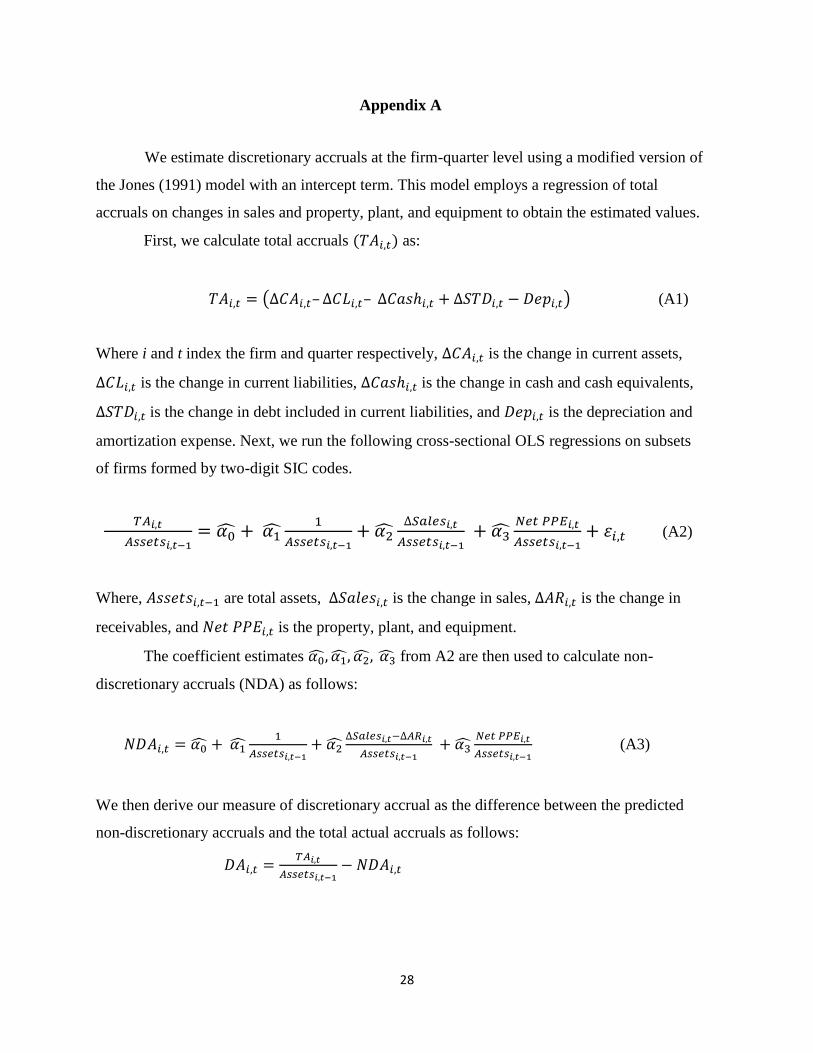
Petroni and Wang, 2010). We calculate quarterly discretionary accruals using the modified Jones

(1991) model that includes an intercept term (the specifics of this methodology are discussed in

Appendix A). We compare the use of discretionary accruals across scandal and non-scandal years by

regressing the absolute value of level of discretionary accruals onto a variety of control variables and

an indicator variable for whether the quarter fell in a scandal year.

11

We include several control variables in the earnings management tests. Following

Summers and Sweeney (1998), we control for standard firm characteristics that could be

related to the fraudulent misstatement of financial statements: Size, growth opportunities

(Market to Book), Leverage, and profitability (ROA). We also control for channels of external

monitoring, as previous literature has shown that outside monitoring affects earnings

management. Yu (2008) finds that firms followed by more analysts manage their earning less.

Institutional investors also play important roles in preventing suspect earnings manipulations

(Shleifer and Vishny, 1986; McConnell and Servaes, 1990; Chung, Firth and Kim 2002).

Therefore, we control for total shares of stock owned by institutional investors (Natural log of

Institutional Ownership) and the number of analysts following the firm (# Analyst Coverage).

Lastly, we control for extreme performance and cash flow volatility by including Growth Rate

of Assets and Cash flow volatility (Dechow and Dichev 2002, Yu 2008).

II.b. Data Sources

We obtain a list of political scandals from Puglisi and Snyder (2008)’s paper “Media Coverage

of Political Scandals.” They collected data on high profile political scandals from 1994 to 2006

involving U.S. senators, congressmen, governors and high-ranking members of public

administrations. These scandals involved various types of wrongful behaviors including

bribery, money laundering and bank fraud. Each of the scandal was investigated by either

federal or state law enforcement agencies. They identify 35 scandals in 19 states. However, in

order to have clearly identified shocks to executives’ attention, it is important to exclude states

that had multiple scandals in a short period of time from the analysis. We therefore focus our

analysis on states that only had one scandal during the sample period. After applying this

restriction, there are 10 scandals in 10 states over the time period 2001 to 2006. We also use

12

the other 32 “scandal-free” states which don’t have any political scandals listed from Puglisi

and Snyder (2008) as the control group.

-Table 1-

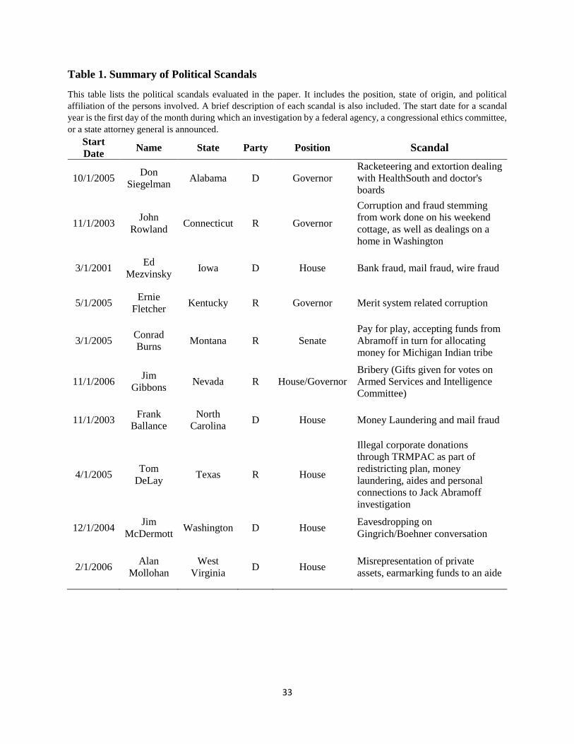
Table 1 provides a brief description of each of the scandals considered, including the

position, state of origin, and political affiliation of the political figures who were implicated.

Following Puglisi and Snyder (2008), we define the start date of a scandal as the first day of

the month when it was revealed that an investigation was being conducted by a federal agency,

a congressional ethics committee, or a state attorney general. A “Scandal Year” refers then to

the 12-month period beginning with the start date of a scandal, and the other years are

considered “Non-Scandal Years”. In order to measure changes in insiders’ trading behavior we

include observations from three years prior to, and two years after, the scandal starting dates.

As a result, the overall time period examined in this paper is from 1999 to 2008. Figure 1

presents a timeline of the begin dates for the scandals during this period.

-Figure 1-

The insider trading data comes from Thomson Reuters. Corporate insiders are required

to report their transactions to the Securities and Exchange Commission (SEC) and their trading

records are available to the public. These insiders include top executives who oversee day-to-

day operations of the firm, directors, and beneficial owners of 10% or more of a company’s

stock. Since we are interested in identifying evidence of illegal trading on private information,

we only evaluate their open market stock purchases and sales. To ensure that news about a

political scandal will be salient, we only include insiders in the sample if they also live in the

state where their firms are headquartered. Trades are aggregated at the firm-month, and trade

13

months are classified as either sale or purchase months based on the aggregate change in

insiders’ positions.

We obtain financial statement information and the addresses for firms’ headquarters

from Compustat, and return data from CRSP. In the final part of our analysis, we consider

whether firms change their financial reporting practices in response to the revelation of a local

political scandal. We use analysts’ forecasts of expected earnings and actual reported earnings

which are available in I/B/E/S for this analysis.

III. Empirical Results

III.A. Profitability of Insider Trades

We have hypothesized that corporate insiders will be less willing to trade on private

information during the year a local political scandal comes to light publicly. In this section, we

compare the abnormal returns following insiders’ trades during the scandal years to those that

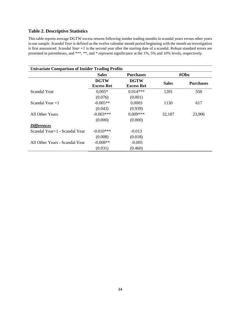
are apparent in non-scandal years. Table 2 reports a univariate analysis of the one-month

abnormal returns following insiders’ trading months. On average, insider sales are followed by

a -0.3% abnormal return in non-scandal years. In contrast, in the year following the

announcements of local political scandals, insiders’ sales are only followed by a 0.5%

abnormal return (the difference is significant at the 10% level). We also contrast the returns

following insiders’ trades during scandal years to those at the same firms in the year after the

scandal. In year t+1 following scandals, insiders’ sales are followed by abnormal returns of -

0.5% which are significantly lower than those following trades in year t at the 5 percent level.

These results indicate that insiders earn smaller abnormal returns in the year following the

14

revelation of local political scandals, but that the contrast is less pronounced in the second year

following the scandals.

A comparison of the abnormal returns following insiders’ purchases tell a different

story. Purchases are followed by positive abnormal returns during non-scandal years (0.9%

overall and 0.03% during year t+1 following a scandal), but they are followed by more

positive abnormal returns of 1.4% during scandal years. These differences, which are

significant at the 1 percent level, are not consistent with insiders being less likely to buy their

stock when they have private positive information when dishonesty is more salient. If

anything, they suggest the opposite.

-Table 2-

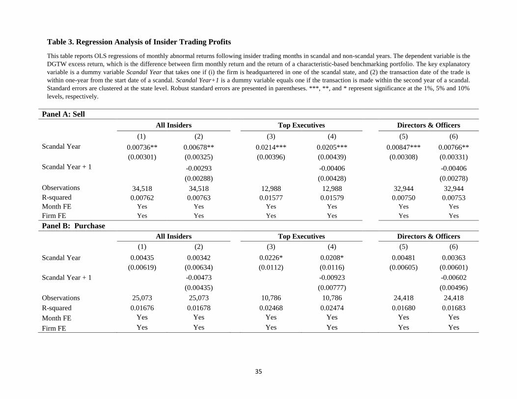
Our analysis continues with multivariate OLS regressions evaluating the returns

following insiders’ trade months in Table 3. To distinguish the treatment group for each

scandal, we include the indicator variable Scandal Year, which equals one if the firm is

headquartered in a scandal state (and the individual also resides in that state), and the

transaction is in the year following the date the scandal is revealed. Since the sample period

spans from 1999 to 2008 and includes firms in various industries, either a time trend or

unobserved firm characteristics could impact the results. We therefore also include both firm

and year fixed effects.

The multivariate regression results for insiders’ sales are reported in Panel A. The

regressions in Column 1 and 2 confirm the univariate results for the returns following insiders’

sales. The coefficients on Scandal Year are about 68 to 74 basis points after the tests include

month and firm effects. The regression in Columns 2 also includes an additional dummy,

Scandal Year + 1, that indicates trades executed in the same state as a scandal but in the

15

second year following it’s revelation. The coefficient on Scandal Year + 1 is negative and

insignificant, suggesting that any impact on executive behavior is limited to the year following

the revelation of the local political scandal. In Columns 3 and 4 we conduct the regressions on

just the sample of trades by top executives (CEO, CFO, COO, GC, President or Chairman of

the Board), and find a stronger effect. The coefficient on Scandal Year is around 2.1% in these

two regressions and each is significant at the 1% level. The larger magnitude of these results

suggests that the saliency of dishonesty has the greatest impact on firms’ top executives. The

samples for the regressions in Columns 5 and 6 are limited to the trades of directors and

officers other than the top executives, and the results are similar to those for the full sample.

Panel B presents a similar analysis of insiders’ purchases. Once we control for month,

and firm effects, the coefficients on Scandal Year are insignificant in the regressions including

the full sample of purchases (Columns 1 and 2) and those that evaluate the trades of directors

and lower level officers (Columns 5 and 6). However, the coefficients on Scandal Year in the

regressions evaluating stock sales by top executives are large and significant. It is 2.26% in the

Column 3 regression, and 2.08% in Column 4. The coefficients on the variable Scandal Year +

1 are insignificant across all specifications, again suggesting that any saliency effect is short-

lived.

-Table 3-

Why might this be the case? A possible explanation may be related to insiders’

incentives to diversify their portfolios if they perceive new limitations on their ability to trade

profitably. Insiders maintain large, undiversified positions in their firms’ stock and they also

have large human capital investments in their firms. One factor in their willingness to maintain

16

large equity stakes may be their ability to adjust that position downward when they receive

information indicating they may face losses. If, once there is an increase in the saliency of

dishonest behavior, they feel constrained in their willingness to sell shares when they have

negative information, then the costs of being undiversified will be higher, and they will have

incentives to limit the size of their positions in their firms. We would therefore only expect

them to purchase their stock when they are confident it will not decline in value, which could

be identified empirically as less buying ahead of price declines.

There is also reason to believe that insiders may be less deterred from purchasing their

shares based on private information when the salience of dishonesty is increased. Other

researchers have argued both that there is greater litigation risk is associated with selling stock

and it is easier to identify harm associated with insiders withholding bad news. If an insider

withholds negative information and trades, other investors will have identifiable losses when

they purchase at an inflated price and the stock subsequently declines in value. However, if an

insider purchases stock on private information, the only harm is to the investors who sold their

shares and therefore weren’t able to enjoy the extra gains the would have realized if the stock

had already reflected the positive information. Insider stock sales can also be used as evidence in

a suit claiming fraudulent financial reporting. However, it is less likely that shareholders will

bring a successful derivative lawsuit claiming insiders fraudulently withheld positive information

because their losses are best described merely as opportunity costs (Skinner, 1994; Brochet,

2010; and Chen, Martin and Wang, 2012).

The next sets of tests we present focus on the relationship between the distribution of

monthly returns and insiders’ trading activity in prior months. This analysis could indicate

whether during scandal years insiders are more likely to purchase shares ahead of price

17

increases, or if they are merely more likely to avoid purchasing ahead of price declines as our

reasoning above would predict. Following that, we test whether insiders change their level of

holdings in their firms following the revelation of a local political scandal. If they are more

likely to reduce their holdings, this would further support our analysis above.

Regardless, it remains possible that an alternative explanation drives the similar

abnormal return patterns that we find for both sales and purchases under these circumstances.

This concern provides additional motivation for our analysis of earnings management

practices. If those results are also in line with our expectations under the salience of dishonesty

hypothesis, it will lend confidence to our interpretation of the insider trading results.

III.B. Likelihood of Trading

It is possible that the results from the prior section reflect differences in the monthly

return distributions across years as opposed to changes in insiders’ willingness to trade on

private information. In this section, we present a supporting analysis that evaluates more

directly whether insiders are less likely to trade when it would be profitable to do so.

Under the assumption that insiders have private information about the expected return

distribution in the following month, we should find a greater likelihood of trading when the

return in the following month is favorable to the trading strategy. Thus, after the outbreak of a

local political scandal, we expect insiders to execute less trades in the direction which would

be profitable.

We start with plotting the distributions of insiders’ trades based on their monthly

returns. As shown in Figure 2, during scandal years, insiders only allocate 22.06% of their

18

sales in the months before a big decline in price (more than 5% decreases), whereas they

execute 6.81% more sales in the months ahead of large decreases in price during non-scandal

years. The chi-square comparing these two frequencies suggests that they are statistically

different at the 1% significance level (Chi(1) =32.58; P-value=0.000). This result indicates that

insiders are less likely to sell before a negative price movement after a local political scandal is

revealed, suggesting less willingness to trade on private information.

The plots for purchase trades have a similar pattern. Insiders are less likely to purchase

before a price decline during scandal years, with a frequency of 17.82% during scandal years

and 28.95% outside of the scandal periods (Chi(1)=32.58; P-value=0.000). In contrast, there is

no evidence showing that insiders are more likely to purchase in the months which would yield

large positive returns (5% or more) during scandal periods. The chi-square is 6.15 and is not

statistically significant with a p-value equals to 0.013. As we predicted, insiders avoid to

purchase ahead of a loss in order to keep their diversification risk low when the willingness of

opportunistic trading is deterred.

-Figure 2-

To further investigate whether insiders trade before the prices move in a favorable

direction, we estimate multivariate linear probability models, predicting the likelihood of

trading when a profitable opportunity is presented. Again, we implement difference-in-

difference framework to focus on the effects on trading behavior that is imposed by the

revelation of a political scandal. In particular, we categorize firm-months into three categories

based on the returns in the following month: (1) the abnormal returns in the following month is

less than -5%; (2) the abnormal returns in the following month is between +5% and -5%; (3)

19

the abnormal returns in the following month is greater than 5%. All calendar firm-months

during the full time period are included as observations in these regressions. We run separate

regressions by defining the dependent variable as a dummy variable which equals 1 if a month

is in one of the above categories, 0 otherwise. Under this setting, we are able to estimate the

likelihood of trading ahead of different return outcomes. We then include a dummy variable

Trade, which equals one if it is a trading month, and 0 other. By interacting Trade with the

dummy variable indicating that the month was during a scandal year, we can determine

whether insiders had a different propensity to trade ahead of different outcomes when

dishonesty was more salient.

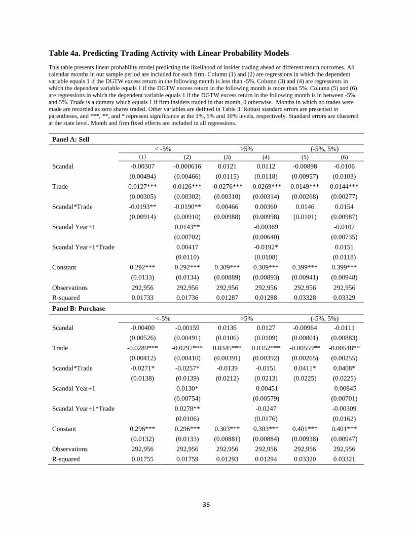
Panel A of Table 4a reports the estimates of the linear probability models. The

insignificant coefficients on Scandal Year*Trade in Columns 3 and 4 show no evidence of a

change in insiders’ selling activity ahead of large positive returns during scandal years.

However, the consistently negative and significant coefficients on Scandal Year*Trade in

Columns 1 and 2 indicate less insider selling ahead of large price declines in scandal years. On

average, insiders are about 2% less likely to sell before the price moves towards a negative

direction (5% significance level).

-Table 4a-

These regressions also include interactions of Scandal Year+1 with the Trade dummy.

The coefficients indicate that in the second year after a scandal breaks local insiders are

actually less likely to sell shares ahead of a large positive return, but the lower level of selling

activity ahead of price declines is no longer apparent. These results are also consistent with

20

those from the returns to trading analysis presented above suggesting that any shift away from

bad behaviors during the scandal years do not persistent.

The patterns shown in the purchase trades confirm our expectations discussed above. In

Panel B of Table 4a, the insignificant coefficients on Scandal Year*Trade across specifications

in columns 3 and 4 indicate that insiders are not purchasing more shares ahead of large positive

returns. In contrast, the negative and significant coefficients on Scandal Year*Trade in

Columns 1 and 2 indicate a decrease in purchasing activity ahead of large price declines in

scandal years. On average, the probability to purchase ahead of an increases in prices are 3%

lower after a local political scandal is revealed. This result is consistent with the observed

distribution in trading and also further confirms our prediction in the prior section.

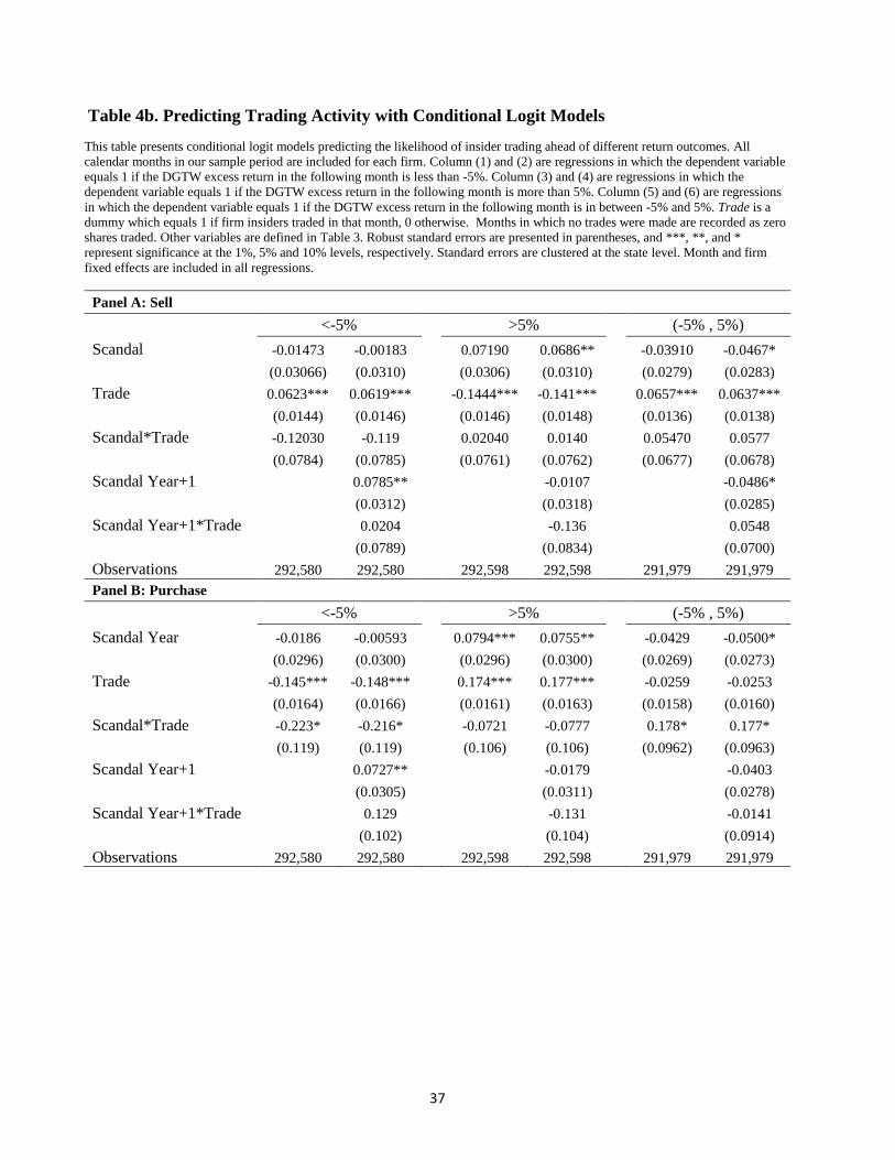
Given that the linear probability model may introduce estimating problems such as

non-normality of the error terms or heteroscedasticity, we also estimate similar regressions

using conditional logit models. As shown in Table 4b, the results are largely consistent with

the ones estimated in the linear probability models.

-Table 4b-

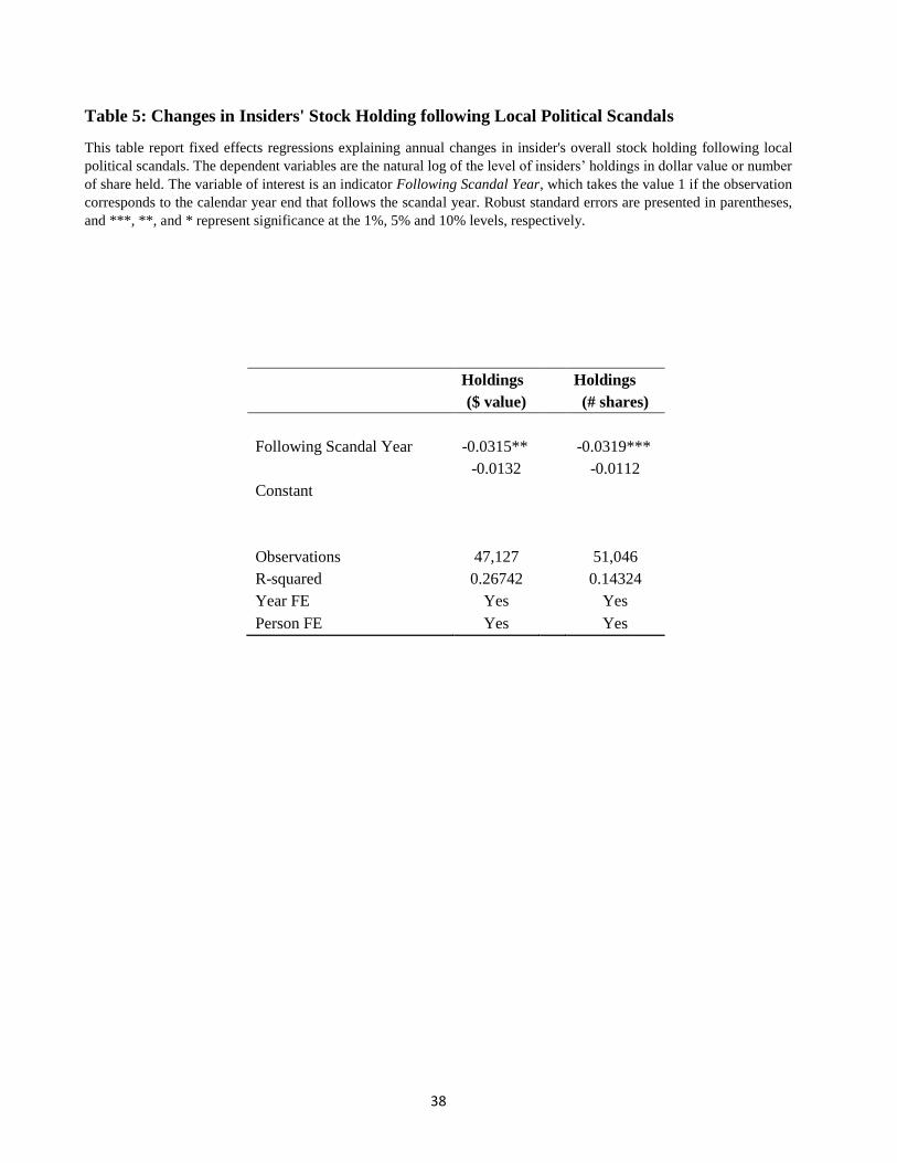
We next consider whether insiders adjust their ownership of their firms’ stock

following the revelation of a local political scandal. As discussed above, we expect that

insiders will diversify away from their companies if they feel restricted in their ability to trade

their stock profitably. Table 5 presents OLS regressions explaining of the natural log of the

number of shares insiders hold (or the dollar value held) that include year and individual fixed

effects. The observations for this test include the calendar year-end holdings for each insider

based on their trading records and stock grants reported in the Thomson data. If insiders are

21

diversifying, we expect their holdings following the scandal year to be lower than in other

years4 The variable of interest is therefore the indicator Following Scandal Year, which takes

the value 1 if the observation corresponds to the calendar year end that follows the scandal

year. The coefficient on this variable is negative and significant in both regressions. The

coefficient of -0.0315 in the first regression indicates that insiders reduce the dollar value of

their holdings by 3.1% during the year. Similarly, the coefficient of -0.0319 in the second

specification indicates a 3.13% reduction in the number of shares they hold.

-Table 5-

III.C. Media Coverage of Scandals and Insider Trading Behavior

The evidence thus far supports a conclusion that corporate insiders are less likely to sell

stock based on private information when the saliency of dishonest behavior is higher. In this

section, we evaluate whether insiders’ trading patterns and returns during scandal years vary as

a function of the level of media coverage of the scandals. This analysis can possibly help rule

out the alternative explanation that local insiders are merely responding to an increase (either

actual or perceived) in the odds of being caught for white collar crime during these time

periods because of higher levels of attention by law enforcement.

We begin by counting the number of local newspaper articles referencing the scandals

in each state. For example, Figure 3 plots the number of articles in Texas newspapers that

reference the scandal involving Tom Delay in each of the twelve months beginning in April,

4 The level of holdings is established using the values reported by insiders on Forms 4 when they are granted

shares or trade. The levels are measured as of calendar year ends due to the great amount of variation in the timing

of trading across months during a year.

22

2005. As would be expected, a large number of articles reference the scandal when Delay’s

ties to lobbyist Jack Abramoff is first reported in April (about 400 articles), but the coverage in

other months ranges from around 150 to over 500 articles on the topic. The highest volumes

of articles came when he was indicted in October, 2005, and when he plead guilty in January,

2006.

-Figure 3-

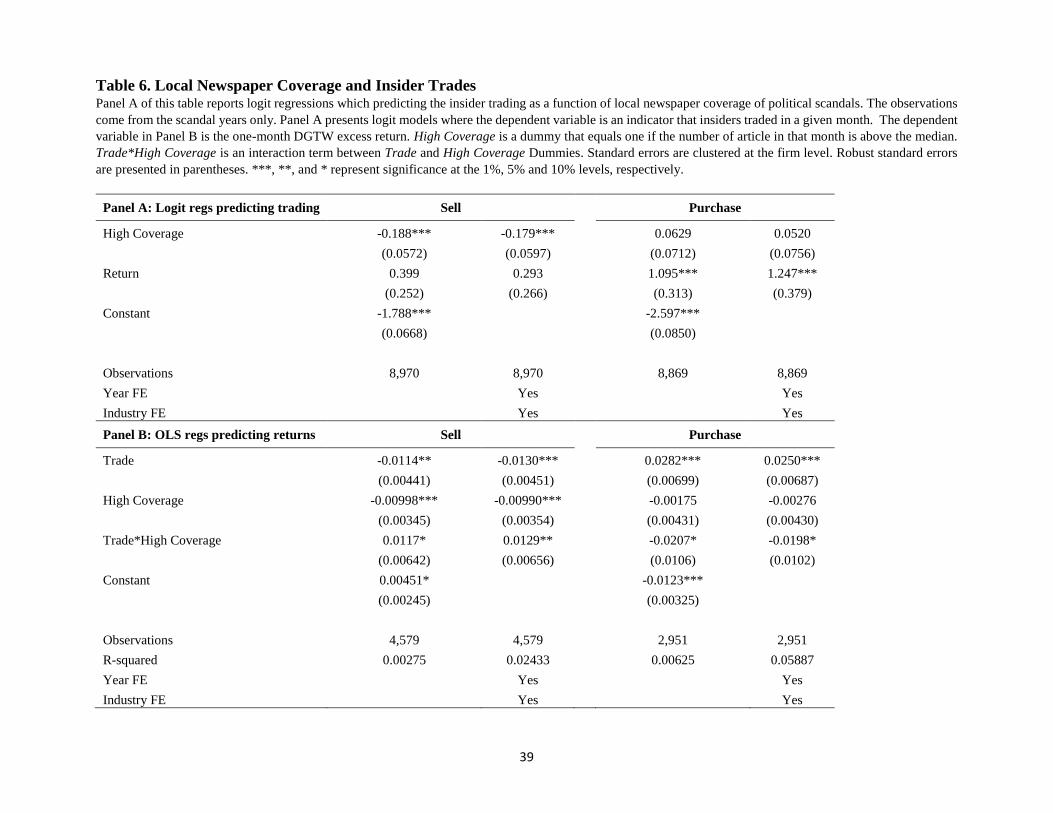
Table 6 presents regressions evaluating whether local insiders behave differently when

there is more news coverage of a political scandal. Panel A reports Logit regressions

explaining the likelihood that insiders trade in months during scandal years as a function of the

level of media coverage, and Panel B reports OLS regressions of the relationship between

media coverage and the returns to insiders’ trades. The logit regressions include as

observations each firm month (12) for each local company in the sample in the scandal year,

and the dummy variable High Coverage indicates if insiders at that firm traded in that month.

The Panel A regressions indicate that insiders are less likely to sell shares in months with

above median media coverage of the local scandal. For example, the coefficient on High

Coverage in column (1) indicates that insiders are 17% less likely to sell shares in a scandal

year month with above median media coverage of the scandal. However, the result is

insignificant with respect to stock purchases.

-Table 6 -

23

The return regressions in Panel B also include as observations each local firm month in

the scandal years.5 Abnormal returns are regressed onto a dummy Trade that indicates that

insiders traded in that month, High Coverage, and the interaction term Trade*High Coverage.

The regressions indicate that when insiders do trade in high media coverage months, the trades

are not as profitable. This can be determined by the significant coefficients on the interaction

term Trade*High Coverage, which is positive and significant in the regressions explaining the

returns to insiders’ sales, and negative and significant in the regressions for purchases. The

returns following sales (purchases) are about 120 bps higher (200 bps lower) when media

coverage is high. The negative and significant coefficient on High Coverage in the regressions

analyzing insiders’ sales also confirms that these months are generally bad for local firms, and

confirm the importance of controlling for this condition separately.

The results discussed in this section indicate that corporate insiders at local firms are

less likely to sell their stock in months when media coverage of scandal-related events is

elevated. The evidence that earn smaller abnormal returns when they do trade their stock in

months with high media coverage suggests that they are less likely to be trading on private

information. These results help to rule out alternative explanations for the main results above

based on expectations of elevated law enforcement because this type of activity would not

likely vary from month to month within the scandal years. These results provide stronger

evidence in favor of the salience of dishonesty hypothesis.

III.E. Earnings Management

5 For the regressions explaining the returns following sales (purchases), firms are only included in the regressions

if at least one of the months could be classified as a sale (purchase) month. This explains the different number of

observations in these regressions.

24

Up to this point, we have shown that suspect insider trading behavior declines after the

revelation of a local political scandal. Those results suggest that insiders modify their personal

behavior in response to an increase in the saliency of dishonest behavior. In this section, we

extend the analysis to consider whether corporate executives also change the way they act on

behalf of their firms under similar circumstances. Our focus is on earnings management,

which, as discussed in the introduction, is one of the more egregious ways that managers may

mislead investors about firm performance and value.

We begin this section with a difference-in-differences analysis of firms’ earnings

surprises. As demonstrated by prior research, firms appear to manage their earnings in order to

just meet or beat analysts’ forecasts in order to either keep investors from pushing their stock

price downward (if they manage earnings up to the threshold) or to reserve slack that can be

used to attain thresholds in the future (when they manage earnings down to the threshold).

Figure 4 plots the distribution of local firms’ quarterly earnings surprises in scandal years

versus other years. A strikingly smaller fraction of surprises in the scandal years either just

meet analysts’ expectations or exceed expectations by 1 penny. It is also evident that firms

report more earnings that either miss expectations by up to 5 cents or exceed expectations by 3

or more cents. These patterns are consistent with prior research showing that firms manage

their earnings either up or down to narrowly attain analysts’ expected earnings.

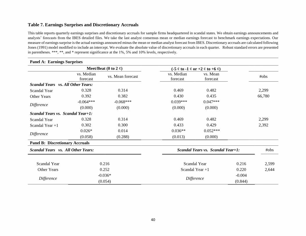
In Panel A of Table 7 we evaluate the statistical significance of these patterns. In years

when scandals are revealed, local firms just meet or beat the median earnings forecast 32.8%

of the time compared to 39.2% of the time in other years, and the difference is statistically

significant at the 1 percent level. Similar results obtain when considering surprises relative to

the mean of analysts’ forecast. The reversed pattern for earnings falling just outside of this

25

window during scandal years is also significant. During scandal years, firms report earnings

that either miss analysts’ expectations by 1 to 5 cents or beat expectations by 2 to 6 cents

approximately 4 percent more often (one percent significance). These results suggest that firms

are less likely to manage earnings into the narrow range of just meeting or beating analysts’

expectations when wrongdoing and its consequences are more salient.

-Figure 4-

We also compare firms’ likelihood of just meeting or beating analysts’ forecasts in

scandal years to the likelihood in the following year. They are actually slightly less likely to

report earnings in this narrow range in the second year after a local scandal is revealed, but the

difference is not statistically significant.

A multivariate regression analysis of earnings surprises is presented in Table 8. Using

both linear probability model and conditional logit model, we predict whether firms report

earnings that meet or just beat earnings forecasts after controlling for common determinants of

earnings surprises identified by prior researchers and discussed in Section 2. We also present

specifications that include quarter and firm fixed effects. The results are largely consistent with

the univariate analysis of earnings surprises. The coefficients on Scandal Year are consistently

negative and significant across all specifications, indicating that local firms are less likely to

report earnings that fall into this narrow range in the year when a political scandal is first

publicized. Consistent with results from insider trades, this effect does not hold in the year

following the scandal year, as evidenced by the insignificant coefficient on Scandal Year + 1 in

all specifications.

-Tables 7 and 8-

26

The greater dispersion of earnings surprises in scandal years suggests that firms are

managing their reported earnings towards targets less aggressively during these years. To

evaluate this proposition further, we analyze firms’ use of discretionary accruals to generate their

reported earnings, a practice that prior researchers have argued may implicate inappropriate

earnings manipulations.

Panel B of Table 7 presents the univariate analyses of discretionary accruals.

Comparing to non-scandal years, firms use less discretionary accruals when a political scandal

is revealed. The difference is 0.036 and significant at 10% level. In Table 9, we observe

similar patterns in discretionary accruals using a multivariate linear regression. The

independent variable of interest is again Scandal Year. The coefficients on Scandal Year are

statistically significant when including common determinants found to be related to the use of

discretionary accruals (Column 2). However, after controlling for firm and quarter fixed

effects, the coefficient on Scandal Year becomes insignificant but remains negative (Column

3). Consistent with earnings surprises, this analysis also suggests that firms are less likely to

manipulate earnings by using greater discretionary accruals in the year following public

revelation of a local political scandal.

-Table 9-

IV. Conclusion

We present evidence that corporate insiders react to the public revelation of the unethical

behaviors of others by acting more honestly themselves. We show that the saliency effect

proposed and supported by Mazar, Amir, and Ariely (2008) and Gino, Ayal, and Ariely (2009)

in their experimental work appears to hold in the real world as well. In particular, corporate

27

insiders appear to execute fewer informed stock sales and to engage in less earnings

management on behalf of their firms after the revelation of a local political scandal. However,

the salience of dishonesty appears to have only a temporary effect on insiders, as the evidence

of informed stock sales and earnings management pick back up in the second year after a

political scandal has been revealed.

This paper furthers our understanding of the reasons why individuals engage in illegal or

antisocial behaviors. It sheds light on whether and how the actions taken by business

professionals reflect the extent to which their attention is drawn to societal rules about the

appropriateness of behavior and the consequences to engaging in illegal actions. It may also

provide guidance on how to develop regulatory or legal regimes that more effectively deter

unwanted behaviors in the business community. For example, it suggests that it be reasonable

to use taxpayer funds to advertise public service announcements in city centers and around

corporate headquarters that remind the public about acts that are illegal or inappropriate. This

tactic -- or other similar alternatives -- may in fact serve as low-cost means of deterring

unwanted and costly behaviors, and, in turn, reduce the cost of investigating and prosecuting

such actions after they occur.

28

Appendix A

We estimate discretionary accruals at the firm-quarter level using a modified version of

the Jones (1991) model with an intercept term. This model employs a regression of total

accruals on changes in sales and property, plant, and equipment to obtain the estimated values.

First, we calculate total accruals (𝑇𝐴𝑖,𝑡) as:

𝑇𝐴𝑖,𝑡 = (∆𝐶𝐴𝑖,𝑡– ∆𝐶𝐿𝑖,𝑡– ∆𝐶𝑎𝑠ℎ𝑖,𝑡 + ∆𝑆𝑇𝐷𝑖,𝑡 − 𝐷𝑒𝑝𝑖,𝑡) (A1)

Where i and t index the firm and quarter respectively, ∆𝐶𝐴𝑖,𝑡 is the change in current assets,

∆𝐶𝐿𝑖,𝑡 is the change in current liabilities, ∆𝐶𝑎𝑠ℎ𝑖,𝑡 is the change in cash and cash equivalents,

∆𝑆𝑇𝐷𝑖,𝑡 is the change in debt included in current liabilities, and 𝐷𝑒𝑝𝑖,𝑡 is the depreciation and

amortization expense. Next, we run the following cross-sectional OLS regressions on subsets

of firms formed by two-digit SIC codes.

𝑇𝐴𝑖,𝑡

𝐴𝑠𝑠𝑒𝑡𝑠𝑖,𝑡−1= 𝛼0̂ + 𝛼1̂

1

𝐴𝑠𝑠𝑒𝑡𝑠𝑖,𝑡−1+ 𝛼2̂

∆𝑆𝑎𝑙𝑒𝑠𝑖,𝑡

𝐴𝑠𝑠𝑒𝑡𝑠𝑖,𝑡−1 + 𝛼3̂

𝑁𝑒𝑡 𝑃𝑃𝐸𝑖,𝑡

𝐴𝑠𝑠𝑒𝑡𝑠𝑖,𝑡−1+ 𝜀𝑖,𝑡 (A2)

Where, 𝐴𝑠𝑠𝑒𝑡𝑠𝑖,𝑡−1 are total assets, ∆𝑆𝑎𝑙𝑒𝑠𝑖,𝑡 is the change in sales, ∆𝐴𝑅𝑖,𝑡 is the change in

receivables, and 𝑁𝑒𝑡 𝑃𝑃𝐸𝑖,𝑡 is the property, plant, and equipment.

The coefficient estimates 𝛼0̂, 𝛼1̂, 𝛼2̂, 𝛼3̂ from A2 are then used to calculate non-

discretionary accruals (NDA) as follows:

𝑁𝐷𝐴𝑖,𝑡 = 𝛼0̂ + 𝛼1̂1

𝐴𝑠𝑠𝑒𝑡𝑠𝑖,𝑡−1+ 𝛼2̂

∆𝑆𝑎𝑙𝑒𝑠𝑖,𝑡−∆𝐴𝑅𝑖,𝑡

𝐴𝑠𝑠𝑒𝑡𝑠𝑖,𝑡−1 + 𝛼3̂

𝑁𝑒𝑡 𝑃𝑃𝐸𝑖,𝑡

𝐴𝑠𝑠𝑒𝑡𝑠𝑖,𝑡−1 (A3)

We then derive our measure of discretionary accrual as the difference between the predicted

non-discretionary accruals and the total actual accruals as follows:

𝐷𝐴𝑖,𝑡 =𝑇𝐴𝑖,𝑡

𝐴𝑠𝑠𝑒𝑡𝑠𝑖,𝑡−1− 𝑁𝐷𝐴𝑖,𝑡

29

References

Agrawal, Anup, and Tommy Cooper, 2015, Insider trading before accounting scandals,

Journal of Corporate Finance 34, 169–190.

Agrawal, Anup, and Tareque Nasser, 2012, Insider trading in takeover targets, Journal of

Corporate Finance 18, 598–625.

Alldredge, Dallin M, and David C Cicero, 2015, Attentive insider trading, Journal of Financial

Economics 115, 84–101.

Bartov, Eli, Dan Givoly, and Carla Hayn, 2002, The rewards to meeting or beating earnings

expectations, Journal of Accounting and Economics 33, 173–204.

Becker, Gary S, 1968, Crime and Punishment: An Economic Approach, Journal of Political

Economy 76, 169–217.

Beny, Laura Nyantung, and H Nejat Seyhun, Has illegal insider trading become more rampant

in the United States? Empirical evidence from takeovers, Research Handbook on

Insider Trading (Edward Elgar Publishing).

Bergstresser, D., and T. Philippon. 2006. CEO incentives and earnings management. Journal of

Financial Economics 80 (3): 511-529.

Bettis, Carr, Don Vickrey, and Donn W Vickrey, 1997, Mimickers of Corporate Insiders Who

Make Large-Volume Trades, Financial Analysts Journal 53, 57–66.

Bhattacharya, U., and H. Daouk, 2002, The World Price of Insider Trading, Journal of

Finance 57, 75-108.

Brochet, Francois, 2010,Information content of insider trades before and after the Sarbanes-

Oxley Act. The Accounting Review 85.2: 419-446.

Bushman, R., J. Piotrioski, and A. Smith, 2005, Insider Trading Restrictions and Analysts’

Incentives to Follow Firms, Journal of Finance 60, 35-66.

Chowdhury, Mustafa, John S Howe, and Ji-Chai Lin, 1993, The Relation between Aggregate

Insider Transactions and Stock Market Returns, The Journal of Financial and

Quantitative Analysis 28, 431.

Chung, Richard, Michael Firth, and Jeong-Bon Kim, 2002, Institutional monitoring and

opportunistic earnings management, Journal of Corporate Finance 8, 29–48.

Cheng, C.S.A., H. H. Huang, and Y. Li, 2013, Does shareholder litigation deter insider

trading?, working paper.

30

Chen, Chen, Xiumin, and Xin Wang, 2012, Insider trading, litigation concerns, and auditor

going-concern opinions, The Accounting Review 88.2 (2012): 365-393.

Cicero, David C, and M Babajide Wintoki, Insider Trading Patterns, SSRN Electronic Journal.

Cohen, L., C. Malloy, and L. Pomorski, 2012, Decoding Inside Information, The Journal of

Finance 67, 1009–1043.

Daniel, K., M. Grinblatt, S. Titman, and R. Wermers, 1997, Measuring Mutual Fund

Performance with Characteristic-Based Benchmarks, The Journal of Finance 52, 1035–

1058.

Dechow, Patricia M, and Ilia D Dichev, 2002, The Quality of Accruals and Earnings: The Role

of Accrual Estimation Errors, The Accounting Review 77, 35–59.

DeFond, M., M. Hung, and R. Trezevant, 2007, Investor Protection and the Information

Content of Annual Earnings Announcements: International Evidence, Journal of

Accounting and Economics 43, 37-67.

Degeorge, Francois, Jayendu Patel, and Richard Zeckhauser, 1999, Earnings Management to

Exceed Thresholds, The Journal of Business 72, 1–33.

Del Guercio, Diane, Elizabeth R. Odders-White, and Mark J. Ready, 2015 ,The Deterrence

Effect of SEC Enforcement Intensity on Illegal Insider Trading: Evidence from Run-up

before News Events, SSRN Electronic Journal.

Fernandes, N., and M. Ferreira, 2009, Insider Trading Laws and Stock Price Informativeness,

Review of Financial Studies 22, 1845-1887.

Finnerty, Joseph E, 1976, Insiders and Market Efficiency, The Journal of Finance 31, 1141.

Gino, Francesca, Shahar Ayal, and Dan Ariely, 2009, Contagion and Differentiation in

Unethical Behavior: The Effect of One Bad Apple on the Barrel, Psychological Science

20, 393–398.

Hayn, Carla, 1995, The information content of losses, Journal of Accounting and Economics

20, 125–153.

Jaffe, Jeffrey F, 1974, Special Information and Insider Trading, The Journal of Business 47,

410.

Jeng, Leslie A, Andrew Metrick, and Richard Zeckhauser, 2003, Estimating the Returns to

Insider Trading: A Performance-Evaluation Perspective, Review of Economics and

Statistics 85, 453–471.

31

Jennings, J., Simi Kedia, and Shivaram Rajgopal, 2011, The detterent effects of SEC

enforcement and class action litigation, SSRN working paper.

Jiang, J, Kathy Petroni and Isabel Wang, 2010, CFOs and CEOs: Who Have the Most

Influence on Earnings Management?. Journal of Financial Economics. 96: 3. 513-526.

Jones, Jennifer J, 1991, Earnings Management During Import Relief Investigations, Journal of

Accounting Research 29, 193.

Karpoff, Jonathan M, D Scott Lee, and Gerald S Martin, 2008, The Cost to Firms of Cooking

the Books, Journal of Financial and Quantitative Analysis 43, 581.

Kasznik, Ron, and Maureen F McNichols, 2002, Does Meeting Earnings Expectations Matter?

Evidence from Analyst Forecast Revisions and Share Prices, J Accounting Res 40,

727–759.

Kedia, S, and T Philippon, 2007, The Economics of Fraudulent Accounting, Review of

Financial Studies 22, 2169–2199.

Kedia, Simi, Kevin Koh, and Shivaram Rajgopal, Evidence on Contagion in Corporate

Misconduct, SSRN Electronic Journal.

Kedia, S., and S. Rajgopal, 2011, Do the SEC’s enforcement preferences affect corporate

misconduct?, Journal of Accounting and Economics, 51, 259-278.

Lakonishok, J, and I Lee, 2001, Are Insider Trades Informative?, Review of Financial Studies

14, 79–111.

Limmack, Robin John, 1985, Analysis of Accounting Statements, Financial Accounting and

Reporting (Springer Science + Business Media).

Lorie, James H, and Victor Niederhoffer, 1968, Predictive and Statistical Properties of Insider

Trading, The Journal of Law and Economics 11, 35–53.

Mazar, Nina, On Amir, and Dan Ariely. 2008. The Dishonesty of Honest People: A Theory of

Self-Concept Maintenance. Journal of Marketing Research Vol. XLV, 633-644.

McConnell, John J, and Henri Servaes, 1990, Additional evidence on equity ownership and

corporate value, Journal of Financial Economics 27, 595–612.

McVay, Sarah, Venky Nagar, and Vicki Wei Tang, 2006, Trading incentives to meet the

analyst forecast, Rev Acc Stud 11, 575–598.

Murphy, Kevin J, 2003, Stock-based pay in new economy firms, Journal of Accounting and

Economics 34, 129–147.

32

Park, Myung Seok, and Taewoo Park, 2004, Insider sales and earnings management, Journal

of Accounting and Public Policy 23, 381–411.

Parsons, Christopher, Johan Sulaeman, and Sheridan Titman, 2014, The Geography of

Financial Misconduct, National Bureau of Economic Research.

Puglisi, Riccardo, and James Snyder, 2008, Media Coverage of Political Scandals, National

Bureau of Economic Research.

Seyhun, H N, 1992, Why Does Aggregate Insider Trading Predict Future Stock Returns?, The

Quarterly Journal of Economics 107, 1303–1331.

Seyhun, H.Nejat, 1986, Insiders’ profits, costs of trading, and market efficiency, Journal of

Financial Economics 16, 189–212.

Seyhun, Hasan Nejat, 2000, Investment Intelligence from Insider Trading (MIT press).

Shleifer, Andrei, and Robert W Vishny, 1986, Large Shareholders and Corporate Control,

Journal of Political Economy 94, 461–488.

Skinner, Douglas J., 1994, Why firms voluntarily disclose bad news. Journal of accounting

research 32.1 (1994): 38-60.

Summers, Scott L, John T Sweeney, and T Sweeney, John, 1998, Fraudulently Misstated

Financial Statements and Insider Trading: An Empirical Analysis, The Accounting

Review 73, 131–146.

Tamersoy, Acar, Bo Xie, Stephen L Lenkey, Bryan R Routledge, Duen Horng Chau, and

Shamkant B Navathe, 2013, Inside insider trading, Proceedings of the 2013 IEEE/ACM

International Conference on Advances in Social Networks Analysis and Mining -

ASONAM ’13 (Association for Computing Machinery (ACM)).

Yu, Fang (Frank), 2008, Analyst coverage and earnings management, Journal of Financial

Economics 88, 245–271.

33

Table 1. Summary of Political Scandals

This table lists the political scandals evaluated in the paper. It includes the position, state of origin, and political

affiliation of the persons involved. A brief description of each scandal is also included. The start date for a scandal

year is the first day of the month during which an investigation by a federal agency, a congressional ethics committee,

or a state attorney general is announced.

Start

Date Name State Party Position Scandal

10/1/2005 Don

Siegelman Alabama D Governor

Racketeering and extortion dealing

with HealthSouth and doctor's

boards

11/1/2003 John

Rowland Connecticut R Governor

Corruption and fraud stemming

from work done on his weekend

cottage, as well as dealings on a

home in Washington

3/1/2001 Ed

Mezvinsky Iowa D House Bank fraud, mail fraud, wire fraud

5/1/2005 Ernie

Fletcher Kentucky R Governor Merit system related corruption

3/1/2005 Conrad

Burns Montana R Senate

Pay for play, accepting funds from

Abramoff in turn for allocating

money for Michigan Indian tribe

11/1/2006 Jim

Gibbons Nevada R House/Governor

Bribery (Gifts given for votes on

Armed Services and Intelligence

Committee)

11/1/2003 Frank

Ballance

North

Carolina D House Money Laundering and mail fraud

4/1/2005 Tom

DeLay Texas R House

Illegal corporate donations

through TRMPAC as part of

redistricting plan, money

laundering, aides and personal

connections to Jack Abramoff

investigation

12/1/2004 Jim

McDermott Washington D House

Eavesdropping on

Gingrich/Boehner conversation

2/1/2006 Alan

Mollohan

West

Virginia D House

Misrepresentation of private

assets, earmarking funds to an aide

34

Table 2. Descriptive Statistics

This table reports average DGTW excess returns following insider trading months in scandal years versus other years

in our sample. Scandal Year is defined as the twelve calendar month period beginning with the month an investigation

is first announced. Scandal Year +1 is the second year after the starting date of a scandal. Robust standard errors are

presented in parentheses, and ***, **, and * represent significance at the 1%, 5% and 10% levels, respectively.

Univariate Comparison of Insider Trading Profits

Sales Purchases #Obs

DGTW

Excess Ret

DGTW

Excess Ret Sales Purchases

Scandal Year 0.005* 0.014*** 1201 550

(0.076) (0.001)

Scandal Year +1 -0.005** 0.0003 1130 617

(0.043) (0.939)

All Other Years -0.003*** 0.009*** 32,187 23,906

(0.000) (0.000)

Differences

Scandal Year+1 - Scandal Year -0.010*** -0.013

(0.008) (0.018)

All Other Years - Scandal Year -0.008** -0.005

(0.031) (0.460)

35

Table 3. Regression Analysis of Insider Trading Profits

This table reports OLS regressions of monthly abnormal returns following insider trading months in scandal and non-scandal years. The dependent variable is the

DGTW excess return, which is the difference between firm monthly return and the return of a characteristic-based benchmarking portfolio. The key explanatory

variable is a dummy variable Scandal Year that takes one if (i) the firm is headquartered in one of the scandal state, and (2) the transaction date of the trade is

within one-year from the start date of a scandal. Scandal Year+1 is a dummy variable equals one if the transaction is made within the second year of a scandal.

Standard errors are clustered at the state level. Robust standard errors are presented in parentheses. ***, **, and * represent significance at the 1%, 5% and 10%

levels, respectively.

Panel A: Sell

All Insiders Top Executives Directors & Officers

(1) (2) (3) (4) (5) (6)

Scandal Year 0.00736** 0.00678** 0.0214*** 0.0205*** 0.00847*** 0.00766**

(0.00301) (0.00325) (0.00396) (0.00439) (0.00308) (0.00331)

Scandal Year + 1 -0.00293 -0.00406 -0.00406

(0.00288) (0.00428) (0.00278)

Observations 34,518 34,518 12,988 12,988 32,944 32,944

R-squared 0.00762 0.00763 0.01577 0.01579 0.00750 0.00753

Month FE Yes Yes Yes Yes Yes Yes

Firm FE Yes Yes Yes Yes Yes Yes

Panel B: Purchase

All Insiders Top Executives Directors & Officers

(1) (2) (3) (4) (5) (6)

Scandal Year 0.00435 0.00342 0.0226* 0.0208* 0.00481 0.00363

(0.00619) (0.00634) (0.0112) (0.0116) (0.00605) (0.00601)

Scandal Year + 1 -0.00473 -0.00923 -0.00602

(0.00435) (0.00777) (0.00496)

Observations 25,073 25,073 10,786 10,786 24,418 24,418

R-squared 0.01676 0.01678 0.02468 0.02474 0.01680 0.01683

Month FE Yes Yes Yes Yes Yes Yes

Firm FE Yes Yes Yes Yes Yes Yes

36

Table 4a. Predicting Trading Activity with Linear Probability Models

This table presents linear probability model predicting the likelihood of insider trading ahead of different return outcomes. All

calendar months in our sample period are included for each firm. Column (1) and (2) are regressions in which the dependent

variable equals 1 if the DGTW excess return in the following month is less than -5%. Column (3) and (4) are regressions in

which the dependent variable equals 1 if the DGTW excess return in the following month is more than 5%. Column (5) and (6)

are regressions in which the dependent variable equals 1 if the DGTW excess return in the following month is in between -5%

and 5%. Trade is a dummy which equals 1 if firm insiders traded in that month, 0 otherwise. Months in which no trades were

made are recorded as zero shares traded. Other variables are defined in Table 3. Robust standard errors are presented in

parentheses, and ***, **, and * represent significance at the 1%, 5% and 10% levels, respectively. Standard errors are clustered

at the state level. Month and firm fixed effects are included in all regressions.

Panel A: Sell

< -5% >5% (-5%, 5%)

(1) (2) (3) (4) (5) (6)

Scandal -0.00307 -0.000616 0.0121 0.0112 -0.00898 -0.0106

(0.00494) (0.00466) (0.0115) (0.0118) (0.00957) (0.0103)

Trade 0.0127*** 0.0126*** -0.0276*** -0.0269*** 0.0149*** 0.0144***

(0.00305) (0.00302) (0.00310) (0.00314) (0.00268) (0.00277)

Scandal*Trade -0.0193** -0.0190** 0.00466 0.00360 0.0146 0.0154

(0.00914) (0.00910) (0.00988) (0.00998) (0.0101) (0.00987)

Scandal Year+1 0.0143** -0.00369 -0.0107

(0.00702) (0.00640) (0.00735)

Scandal Year+1*Trade 0.00417 -0.0192* 0.0151

(0.0110) (0.0108) (0.0118)

Constant 0.292*** 0.292*** 0.309*** 0.309*** 0.399*** 0.399***

(0.0133) (0.0134) (0.00889) (0.00893) (0.00941) (0.00948)

Observations 292,956 292,956 292,956 292,956 292,956 292,956

R-squared 0.01733 0.01736 0.01287 0.01288 0.03328 0.03329

Panel B: Purchase

<-5% >5% (-5%, 5%)

Scandal -0.00400 -0.00159 0.0136 0.0127 -0.00964 -0.0111

(0.00526) (0.00491) (0.0106) (0.0109) (0.00801) (0.00883)

Trade -0.0289*** -0.0297*** 0.0345*** 0.0352*** -0.00559** -0.00548**

(0.00412) (0.00410) (0.00391) (0.00392) (0.00265) (0.00255)

Scandal*Trade -0.0271* -0.0257* -0.0139 -0.0151 0.0411* 0.0408*

(0.0138) (0.0139) (0.0212) (0.0213) (0.0225) (0.0225)

Scandal Year+1 0.0130* -0.00451 -0.00845

(0.00754) (0.00579) (0.00701)

Scandal Year+1*Trade 0.0278** -0.0247 -0.00309

(0.0106) (0.0176) (0.0162)

Constant 0.296*** 0.296*** 0.303*** 0.303*** 0.401*** 0.401***

(0.0132) (0.0133) (0.00881) (0.00884) (0.00938) (0.00947)

Observations 292,956 292,956 292,956 292,956 292,956 292,956

R-squared 0.01755 0.01759 0.01293 0.01294 0.03320 0.03321

37

Table 4b. Predicting Trading Activity with Conditional Logit Models

This table presents conditional logit models predicting the likelihood of insider trading ahead of different return outcomes. All

calendar months in our sample period are included for each firm. Column (1) and (2) are regressions in which the dependent variable

equals 1 if the DGTW excess return in the following month is less than -5%. Column (3) and (4) are regressions in which the

dependent variable equals 1 if the DGTW excess return in the following month is more than 5%. Column (5) and (6) are regressions

in which the dependent variable equals 1 if the DGTW excess return in the following month is in between -5% and 5%. Trade is a

dummy which equals 1 if firm insiders traded in that month, 0 otherwise. Months in which no trades were made are recorded as zero

shares traded. Other variables are defined in Table 3. Robust standard errors are presented in parentheses, and ***, **, and *

represent significance at the 1%, 5% and 10% levels, respectively. Standard errors are clustered at the state level. Month and firm

fixed effects are included in all regressions.

Panel A: Sell

<-5% >5% (-5% , 5%)

Scandal -0.01473 -0.00183 0.07190 0.0686** -0.03910 -0.0467*

(0.03066) (0.0310) (0.0306) (0.0310) (0.0279) (0.0283)

Trade 0.0623*** 0.0619*** -0.1444*** -0.141*** 0.0657*** 0.0637***

(0.0144) (0.0146) (0.0146) (0.0148) (0.0136) (0.0138)

Scandal*Trade -0.12030 -0.119 0.02040 0.0140 0.05470 0.0577

(0.0784) (0.0785) (0.0761) (0.0762) (0.0677) (0.0678)

Scandal Year+1 0.0785** -0.0107 -0.0486*

(0.0312) (0.0318) (0.0285)

Scandal Year+1*Trade 0.0204 -0.136 0.0548

(0.0789) (0.0834) (0.0700)

Observations 292,580 292,580 292,598 292,598 291,979 291,979

Panel B: Purchase

<-5% >5% (-5% , 5%)

Scandal Year -0.0186 -0.00593 0.0794*** 0.0755** -0.0429 -0.0500*

(0.0296) (0.0300) (0.0296) (0.0300) (0.0269) (0.0273)

Trade -0.145*** -0.148*** 0.174*** 0.177*** -0.0259 -0.0253

(0.0164) (0.0166) (0.0161) (0.0163) (0.0158) (0.0160)

Scandal*Trade -0.223* -0.216* -0.0721 -0.0777 0.178* 0.177*

(0.119) (0.119) (0.106) (0.106) (0.0962) (0.0963)

Scandal Year+1 0.0727** -0.0179 -0.0403

(0.0305) (0.0311) (0.0278)

Scandal Year+1*Trade 0.129 -0.131 -0.0141

(0.102) (0.104) (0.0914)

Observations 292,580 292,580 292,598 292,598 291,979 291,979

38

Table 5: Changes in Insiders' Stock Holding following Local Political Scandals

This table report fixed effects regressions explaining annual changes in insider's overall stock holding following local

political scandals. The dependent variables are the natural log of the level of insiders’ holdings in dollar value or number

of share held. The variable of interest is an indicator Following Scandal Year, which takes the value 1 if the observation

corresponds to the calendar year end that follows the scandal year. Robust standard errors are presented in parentheses,

and ***, **, and * represent significance at the 1%, 5% and 10% levels, respectively.

Holdings Holdings

($ value) (# shares)

Following Scandal Year -0.0315** -0.0319***

-0.0132 -0.0112

Constant

Observations 47,127 51,046

R-squared 0.26742 0.14324

Year FE Yes Yes

Person FE Yes Yes

39

Table 6. Local Newspaper Coverage and Insider Trades Panel A of this table reports logit regressions which predicting the insider trading as a function of local newspaper coverage of political scandals. The observations

come from the scandal years only. Panel A presents logit models where the dependent variable is an indicator that insiders traded in a given month. The dependent

variable in Panel B is the one-month DGTW excess return. High Coverage is a dummy that equals one if the number of article in that month is above the median.

Trade*High Coverage is an interaction term between Trade and High Coverage Dummies. Standard errors are clustered at the firm level. Robust standard errors

are presented in parentheses. ***, **, and * represent significance at the 1%, 5% and 10% levels, respectively.

Panel A: Logit regs predicting trading Sell Purchase

High Coverage -0.188*** -0.179*** 0.0629 0.0520

(0.0572) (0.0597) (0.0712) (0.0756)

Return 0.399 0.293 1.095*** 1.247***

(0.252) (0.266) (0.313) (0.379)

Constant -1.788*** -2.597***

(0.0668) (0.0850)

Observations 8,970 8,970 8,869 8,869

Year FE Yes Yes

Industry FE Yes Yes

Panel B: OLS regs predicting returns Sell Purchase

Trade -0.0114** -0.0130*** 0.0282*** 0.0250***

(0.00441) (0.00451) (0.00699) (0.00687)

High Coverage -0.00998*** -0.00990*** -0.00175 -0.00276

(0.00345) (0.00354) (0.00431) (0.00430)

Trade*High Coverage 0.0117* 0.0129** -0.0207* -0.0198*

(0.00642) (0.00656) (0.0106) (0.0102)

Constant 0.00451* -0.0123***

(0.00245) (0.00325)

Observations 4,579 4,579 2,951 2,951

R-squared 0.00275 0.02433 0.00625 0.05887

Year FE Yes Yes

Industry FE Yes Yes

40

Table 7. Earnings Surprises and Discretionary Accruals

This table reports quarterly earnings surprises and discretionary accruals for sample firms headquartered in scandal states. We obtain earnings announcements and

analysts’ forecasts from the IBES detailed files. We take the last analyst consensus mean or median earnings forecast to benchmark earnings expectations. Our

measure of earnings surprise is the actual earnings announced minus the mean or median analyst forecast from IBES. Discretionary accruals are calculated following

Jones (1991) model modified to include an intercept. We evaluate the absolute value of discretionary accruals in each quarter. Robust standard errors are presented

in parentheses. ***, **, and * represent significance at the 1%, 5% and 10% levels, respectively.

Panel A: Earnings Surprises

Meet/Beat (0 to 2 ¢) (-5 ¢ to -1 ¢ or +2 ¢ to +6 ¢)

vs. Median

forecast vs. Mean forecast

vs. Median

forecast

vs. Mean

forecast #obs

Scandal Years vs. All Other Years:

Scandal Year 0.328 0.314 0.469 0.482 2,299

Other Years 0.392 0.382 0.430 0.435 66,780

Difference -0.064*** -0.068*** 0.039*** 0.047***

(0.000) (0.000) (0.000) (0.000)

Scandal Years vs. Scandal Year+1:

Scandal Year 0.328 0.314 0.469 0.482 2,299

Scandal Year +1 0.302 0.300 0.433 0.429 2,392

Difference 0.026* 0.014 0.036** 0.052***

(0.058) (0.288) (0.013) (0.000)

Panel B: Discretionary Accruals

Scandal Years vs. All Other Years: Scandal Years vs. Scandal Year+1: #obs

Scandal Year 0.216 Scandal Year 0.216 2,599

Other Years 0.252 Scandal Year +1 0.220 2,644

Difference -0.036*

Difference -0.004

(0.054) (0.844)

41

Table 8. Regression Analysis of Earnings Surprises

This Table presents linear probability regressions and conditional logit regressions of BEAT (an indicator that a firm reported a quarterly earnings surprise of 0¢,

1¢ or 2¢) onto independent variables that control for firm characteristics. The sample of observation includes earnings announcements from 1999 to 2008. Earnings

surprises are calculated as the difference between firm actual earnings and analysts’ consensus median forecast. Scandal Year is an indicator variable equals one if

observations are in the first four quarters (0, 1, 2, and 3) after revelation of a political scandal. Scandal Year+1 equals one for the second four quarters (4, 5, 6, 7)

after a scandal is first publicized. Size is the nature log of market cap. Market to Book is the natural log of market to book ratio. ROA is the return on assets. # of

analyst coverage is the number of analyst covering the firm. Institutional Ownership is the natural log of total share of stock owned by institutional investor.

Leverage is calculated as total liabilities scaled by total assets. Growth rate of assets is calculated by the change of assets scaled by lagged assets. Cash flow

volatility is estimated by standard deviations of cash flow of a firm in the entire sample period, scaled by lagged assets. All non-binary independent variables are

lagged one year. Robust standard errors in parentheses***, **, and * represent significance at the 1%, 5% and 10% levels, respectively.

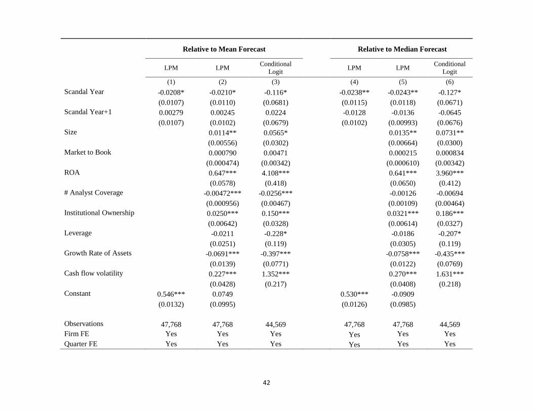
42

Relative to Mean Forecast

Relative to Median Forecast

LPM LPM Conditional

Logit LPM LPM

Conditional

Logit

(1) (2) (3) (4) (5) (6)

Scandal Year -0.0208* -0.0210* -0.116* -0.0238** -0.0243** -0.127*

(0.0107) (0.0110) (0.0681) (0.0115) (0.0118) (0.0671)

Scandal Year+1 0.00279 0.00245 0.0224 -0.0128 -0.0136 -0.0645

(0.0107) (0.0102) (0.0679) (0.0102) (0.00993) (0.0676)

Size 0.0114** 0.0565* 0.0135** 0.0731**

(0.00556) (0.0302) (0.00664) (0.0300)

Market to Book 0.000790 0.00471 0.000215 0.000834

(0.000474) (0.00342) (0.000610) (0.00342)

ROA 0.647*** 4.108*** 0.641*** 3.960***

(0.0578) (0.418) (0.0650) (0.412)

# Analyst Coverage -0.00472*** -0.0256*** -0.00126 -0.00694

(0.000956) (0.00467) (0.00109) (0.00464)

Institutional Ownership 0.0250*** 0.150*** 0.0321*** 0.186***

(0.00642) (0.0328) (0.00614) (0.0327)

Leverage -0.0211 -0.228* -0.0186 -0.207*

(0.0251) (0.119) (0.0305) (0.119)

Growth Rate of Assets -0.0691*** -0.397*** -0.0758*** -0.435***

(0.0139) (0.0771) (0.0122) (0.0769)

Cash flow volatility 0.227*** 1.352*** 0.270*** 1.631***

(0.0428) (0.217) (0.0408) (0.218)

Constant 0.546*** 0.0749 0.530*** -0.0909

(0.0132) (0.0995) (0.0126) (0.0985)

Observations 47,768 47,768 44,569 47,768 47,768 44,569

Firm FE Yes Yes Yes Yes Yes Yes

Quarter FE Yes Yes Yes Yes Yes Yes

43

Table 9. Regression Analysis of Discretionary Accruals

This Table presents OLS regressions of discretionary accruals onto independent variables that control for firm characteristics. The sample of observation includes

earnings announcements for firm quarters from 1999 to 2008. Discretionary accruals are calculated following Jones (1991) modified model that includes an

intercept. Scandal Year is an indicator variable equals one if observations are in the first four quarters (0,1,2,3) after a political scandal is first reported. Scandal

Year+1 equals one for the second four quarters (0,1,2,3) after a scandal is first publicized. Size is the nature log of market cap. Market to Book is the natural log of

market to book ratio. ROA is the return on assets. # of analyst coverage is the number of analyst covering the firm. Institutional Ownership is the natural log of

total share of stock owned by institutional investor. Leverage is calculated as total liabilities scaled by total assets. Growth rate of assets is calculated by the change

of assets scaled by lagged assets. Cash flow volatility is estimated by standard deviations of cash flow of a firm in the entire sample period, scaled by lagged assets.

All non-binary independent variables are lagged one year. Robust standard errors in parentheses***, **, and * represent significance at the 1%, 5% and 10% levels,

respectively.

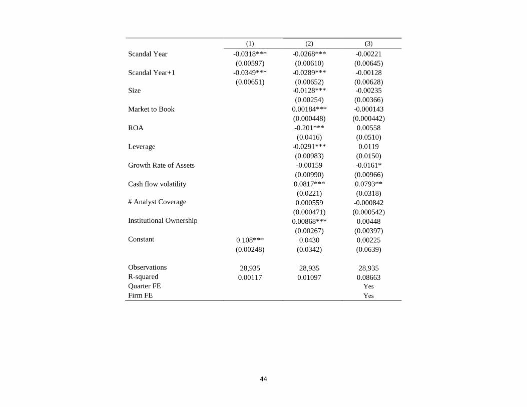
44

(1) (2) (3)

Scandal Year -0.0318*** -0.0268*** -0.00221

(0.00597) (0.00610) (0.00645)

Scandal Year+1 -0.0349*** -0.0289*** -0.00128

(0.00651) (0.00652) (0.00628)

Size -0.0128*** -0.00235

(0.00254) (0.00366)

Market to Book 0.00184*** -0.000143

(0.000448) (0.000442)

ROA -0.201*** 0.00558

(0.0416) (0.0510)

Leverage -0.0291*** 0.0119

(0.00983) (0.0150)

Growth Rate of Assets -0.00159 -0.0161*

(0.00990) (0.00966)

Cash flow volatility 0.0817*** 0.0793**

(0.0221) (0.0318)

# Analyst Coverage 0.000559 -0.000842

(0.000471) (0.000542)

Institutional Ownership 0.00868*** 0.00448

(0.00267) (0.00397)

Constant 0.108*** 0.0430 0.00225

(0.00248) (0.0342) (0.0639)

Observations 28,935 28,935 28,935

R-squared 0.00117 0.01097 0.08663

Quarter FE Yes

Firm FE Yes

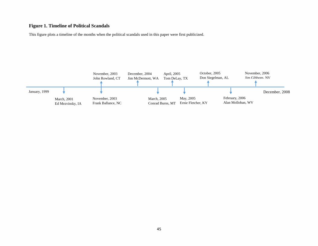
45

Figure 1. Timeline of Political Scandals

This figure plots a timeline of the months when the political scandals used in this paper were first publicized.

March, 2001

Ed Mezvinsky, IA

November, 2003

John Rowland, CT

November, 2003

Frank Ballance, NC

December, 2004

Jim McDermott, WA

March, 2005

Conrad Burns, MT

April, 2005

Tom DeLay, TX

May, 2005

Ernie Fletcher, KY

October, 2005

Don Siegelman, AL

February, 2006

Alan Mollohan, WV

November, 2006

Jim Gibbons, NV

January, 1999 December, 2008

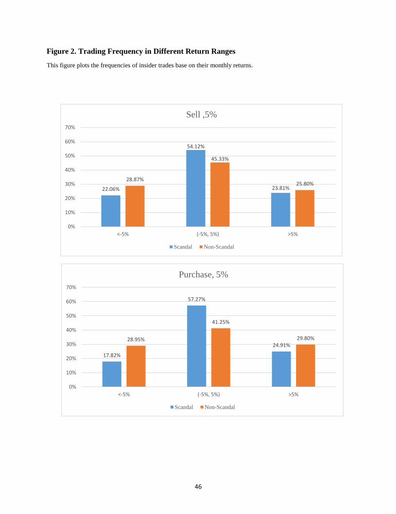
46

Figure 2. Trading Frequency in Different Return Ranges

This figure plots the frequencies of insider trades base on their monthly returns.

22.06%

54.12%

23.81%

28.87%

45.33%

25.80%

0%

10%

20%

30%

40%

50%

60%

70%

<-5% (-5%, 5%) >5%

Sell ,5%

Scandal Non-Scandal

17.82%

57.27%

24.91%28.95%

41.25%

29.80%

0%

10%

20%

30%

40%

50%

60%

70%

<-5% (-5%, 5%) >5%

Purchase, 5%

Scandal Non-Scandal

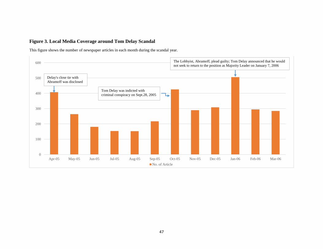
47

Figure 3. Local Media Coverage around Tom Delay Scandal

This figure shows the number of newspaper articles in each month during the scandal year.

0

100

200

300

400

500

600

Apr-05 May-05 Jun-05 Jul-05 Aug-05 Sep-05 Oct-05 Nov-05 Dec-05 Jan-06 Feb-06 Mar-06

No. of Article

Delay's close tie with

Abramoff was disclosed

Tom Delay was indicted with

criminal conspiracy on Sept.28, 2005

The Lobbyist, Abramoff, plead guilty; Tom Delay announced that he would

not seek to return to the position as Majority Leader on January 7, 2006

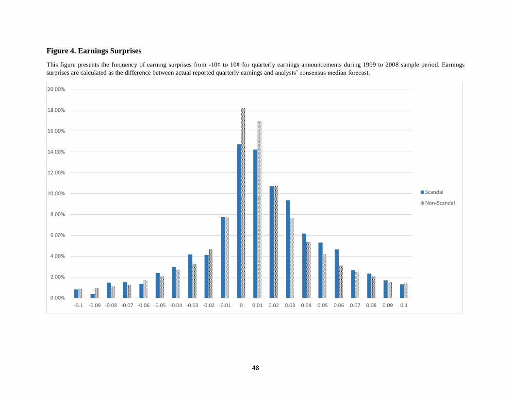
48

Figure 4. Earnings Surprises

This figure presents the frequency of earning surprises from -10¢ to 10¢ for quarterly earnings announcements during 1999 to 2008 sample period. Earnings

surprises are calculated as the difference between actual reported quarterly earnings and analysts’ consensus median forecast.

0.00%

2.00%

4.00%

6.00%

8.00%

10.00%

12.00%

14.00%

16.00%

18.00%

20.00%

-0.1 -0.09 -0.08 -0.07 -0.06 -0.05 -0.04 -0.03 -0.02 -0.01 0 0.01 0.02 0.03 0.04 0.05 0.06 0.07 0.08 0.09 0.1

Scandal

Non-Scandal