Embed Size (px)
Citation preview
Do Executive Stock Options Generate Incentives for Earnings Management? Evidence
from Accounting Restatements 1
Simi Kedia
Harvard Business School & Ohio State University Tel: (614) 292-0363 Fax: (614) 292-2418
E-mail: [email protected]
First Draft: March 2003 This Draft: October 2003
Abstract
In a sample of 224 firms that announced restating their financial statements from January 1997 to June 2002 due to accounting irregularities and a control group of all non-restating firms with data on ExecuComp, we examine the effect of pay for performance incentives on the incentives for earnings management. Controlling for the endogeneity of pay for performance incentives, we find a significant positive effect of incentives on the probability of restating. In our sample, average value of executive option holdings increases by $21 for every $1000 change in equity value. Increasing incentives by 90 cents or 4.3% from the above mean increases the probability of restatement by 1%. We find that stock and options differ in the incentives generated for earnings management. There is no evidence that equity holdings generate incentives for earnings management. Further, large managerial ownership mitigates the positive effect of stock options on the incentive to manage earnings.
Keywords: Executive Stock Options, Compensation, Accounting Restatements, Earnings Management.
1 I would like to thank Kose John, Nagpurnanand Prabhala, Jeremy Stein, Siew Hong Teoh, Ralph Walking, Karen Wruck, David Yermack, participants at the 2003 NBER Universities Research Conference on Corporate Governance, and seminar participants at Indiana University, University of Georgetown, and Ohio State University for their comments. I would like to thank Kim Haufrect for excellent research assistance and the General Account Office for sharing the data on announcements of restatements. I gratefully acknowledge financial support from the Division of Research at the Harvard Business School. All errors are mine.

Principal-agent theory suggests that stock-based compensation is one of the natural
mechanisms to tie manager’s pay to firm performance and therefore give him incentives to
take actions, often unobservable, in line with shareholder wealth maximization. Since
Jensen and Murphy (1990) documented that despite this central tenet of the principal-agent
theories, the pay for performance sensitivities of CEOs in modern corporations remains low,
there has been a surge in the use of stock options for compensating executives (See Hall and
Leibman (1998), Murphy (1999)).
As managerial pay for performance incentives have increased, managerial wealth is
increasing sensitive to firm performance. This increasing sensitivity of managerial wealth to
firm performance focuses managerial attention on share price. This focus on share price has
the intended affect of making managers choose actions that increase firm’s intrinsic value.
However, it may also have the unintended effect of making managers choose actions that will
increase the share price irrespective of its effect on the firm’s intrinsic value. Understanding
these unintended consequences of pay for performance incentives is important to inform the
predictions of agency theory and design efficient compensation mechanisms.
In this paper, we examine one such unintended consequence of increasing pay for
performance incentives of managers. Earnings manipulation is one example where
aggressive accounting practices may allow managers to prop up the share price by reporting
performance estimates that do not accurately reflect the firm’s underlying economics.2 We
study a very specific instance of this possible incentive to “manage earnings” by examining
firms that restate their financial statements due to accounting irregularities over the period
2 Another example of the unintended effects of stock options is on the incentives to manipulate voluntary disclosures. Aboody and Kasznik (2000) document that managers delay the announcement of good news and rush the announcement of bad news. Such a disclosure strategy ensures that negative price reactions to bad news occur before option awards and positive price reactions to good news after option grants.
2
January 1997 to June 2002. This sample of restating firms is based on a Lexis Nexus search
and was compiled by the General Accounting Office (GAO) for a study of accounting
restatements requested by the Chairman, Committee on Banking, Housing and Urban Affairs
of the U.S. Senate. This list of 919 announcements of restatements includes only
restatements due to accounting irregularities. We match this list of restating firms to firms for
which compensation data is available on ExecuComp to obtain a sample of 224 unique firms
that make 257 announcements of restatements.
We estimate the probability of a firm restating its financial statement with pay for
performance incentives as an endogenous explanatory behavior. Pay for performance
incentives are measured as, 1) the change in the value of stock options held for a dollar
change in equity value, and 2) the change in the value of stock options held for a percentage
change in equity value. We also control for other motivations of earnings management
proposed in prior literature. In particular, we control for the incentives to manage earnings
arising from debt covenants, pressure to maintain earnings momentum, beat analyst forecasts,
firm characteristics and weak governance.
We examine incentives for the top five executives in the years prior to the
announcement of the restatement, i.e., for the years prior to and during the alleged
manipulation. We find significant evidence that pay for performance incentives are
endogenous. Controlling for endogeneity, pay for performance incentives from stock options
have a significant positive effect on the probability of restatement. This effect is both
statistically and economically significant. In our sample, average value of executive option
holdings increases by $21 for every $1000 increase in equity value. Increasing incentives by
90 cents or 4.3% from the above mean increases the probability of restatement by 1%. Using
3

the second measure, we find that average value of executive option holdings increases by
$446,000 for every 1% increase in equity value. Increasing these incentives by $52,000 or
11.7% increases the probability of restatement by 1%. Firm characteristics also significantly
effect the probability of restatement. There is little evidence in our sample to support the
other proposed motivations of earnings management.
We find that stock and options differ in the incentives generated for earnings
management, though both provide pay for performance incentives. There is no evidence that
equity holdings generate any incentive to manage earnings. Further, large equity holdings
by managers are found to mitigate the positive effect of stock options on the incentive to
manage earnings. This difference between stock and stock options might be due to control
benefits associated with large equity stakes. Executives with large equity stakes are not likely
to unwind their holdings to realize gains from a higher stock price achieved as a result of
earnings management. As these executives bear the expected costs of earnings management,
their motivation for managing earnings is likely to be lower.
The remainder of the paper is organized as follows. We examine related literature in
Section II, describe our sample in Section III, and discuss the econometric and economic
model in Sections IV and V respectively. We present results in Section VI, discuss the effect
of managerial ownership in Section VII, and conclude in Section VIII.
II. Earnings Management and Related Literature
Healy (1986) first documented that accruals are related to managerial bonus schemes.
Subsequently, Dechow, Sloan and Sweeney (1996) and Beneish (1999) examine the effect of
gains from insider sales as a motivation of earning management in a sample of firms that are
charged by SEC of violating Generally Accepted Accounting Principles (GAAP). Though
4
Beneish (1999) finds that gains from stock sales are a factor motivating earnings
management, Dechow et al (1996) find no such evidence. These papers do not examine the
effect of pay for performance incentives partly due to their sample predating the rapid rise in
these incentives.3
Some recent papers ask questions similar to ours but take different approaches.
Bergstresser and Philippon (2002) use accruals to proxy for earnings management and find
that the use of discretionary accruals is more pronounced in firms where stock options
constitute a larger fraction of CEO compensation. Johnson, Ryan and Tian (2003) examine a
sample of firms charged of GAAP violations by the SEC and also find evidence of higher
equity based incentives in these firms. Burns (2003) finds evidence that CEO incentives
affect the probability of restatement.4 Bar-Gill and Bebchuck (2003) develop a model for the
incentives to misreport corporate performance. Agarwal and Chadha (2002) also examine a
sample of restating firms but study the effect of board characteristics on the probability of
restatement.
Prior literature has used estimates of abnormal or unexpected accruals to detect and
capture earnings management. Pay for performance incentives will effect earnings
management only if earnings management has price effects. It is not clear when accruals can
be regarded as abnormal or unexpected. If capital markets see through accruals then they
should have no price effects. In contrast, there is no doubt that restatements have a price
effect. The GAO (2002) study documents - 10% return over two days around announcement
of restatements. This makes restatements a desirable venue to examine the effect of pay for
3 Beneish (1999) does find evidence of higher exercises of stock appreciation rights (SARs) in firms charged by SEC of GAAP violations. 4 Burns (2003) has a sample very similar to ours. Our papers differs in: 1) methodology as we correct for the endogeneity of incentives, and 2) she examine CEO incentives while we study the incentives of the executive team.
5

performance incentives on earnings management. As our sample consists of firms that
announce restatements due to accounting irregularities, it focuses our attention on the errant
firm rather than on the firm that has “legitimate” high accruals (or of having to fit a model of
“abnormal” accruals).5 An alternate way to study earnings management is to examine a
sample of firms that are charged of GAAP violations by the SEC. This has the advantage of
selecting firms that have a higher probability of having managed earnings. Though this
increases the power of tests it limits the generalizibility of results to less obvious forms of
earnings management that have been widespread over this time period.
III. Sample Selection and Data Description
The General Accounting Office (GAO) October 2002 report to the Chairman,
Committee on Banking, Housing and Urban Affairs of the U.S. Senate, titled “Financial
Statement Restatements: Trends, Market Impacts, Regulatory Response, and Remaining
Challenges,” identifies 919 announcements of accounting restatements by 845 firms over the
period January 1997 to June 30, 2002. These announcements were identified by the GAO
through a Lexus-Nexus search with variations of the word ‘restate’. These announced
restatements were due to accounting irregularities resulting in material misstatements of
financial reports.6 I use this list as the basis of this study.
5 Richardson et. al (2002) find that firms that restate have large accruals. This does not however imply that all firms with large accruals will restate. Restatements thus allow us a natural way to identify dramatic and “irregular” cases of earnings management. 6 GAO defined accounting irregularity as an instance where the company restates is financial statements because they were not fairly presented in accordance with GAAP. This includes material errors as well as fraud. Portions of this list were cross-checked with lists compiled by the SEC, the Congressional Research Service and others at the GAO, when this information was available. As many restatements are routine and on account of acquisitions, divestitures and other corporate restructuring activities, it is important to isolate the firms that restate due of accounting irregularities. Wu (2002) also identifies a similar sample over a different time period, 1971-2000.
6
I match these 845 firms with the firms included in the ExecuComp database to get a
sample of firms for which compensation data is available. Of the 845 firms, 224 firms were
covered in ExecuComp. These 224 firms make 257 announcements of restatements. The
distribution of these restatement announcements over time for sample firms and the GAO
sample is displayed in Table 1. For firms that make multiple announcements we include only
the first announcement. As compensation often comes under intense scrutiny after the
announcement of a restatement the years after the first announcement and before the second
announcement may not be representative of the pre-detection compensation effects we would
like to document.
Data on options and stock outstanding for the top five most highly paid executives
were obtained from ExecuComp. Data on compensation for the individual executives was
aggregated to obtain firm level values of options to be referred to as executive compensation
from now on. We focus on the pay for performance incentives of all five executives, as
opposed to only CEO incentives. Managing earnings most likely requires consent and
participation of at least some of executives other than the CEO.7 To the extent that we
include executives not involved in earnings management we potentially bias the results
against us.
As we wish to study the effect of pay for performance incentives on the incentives to
manage earnings, we focus on incentives in place prior to and during the period of earnings
management. We include the year prior to the years of alleged manipulation, as managers
are likely to enter the earnings management years with high incentives. The incentives in
place prior to the manipulation might explain the decision to manage earnings to begin with.
7 This has been borne out in several cases like Enron, Tyco where executives other than the CEO were involved. Section 302 of the Sarbanes-Oxley (2002) act requires CEO and CFO certification of quarterly financial statements also pointing to the importance of executives, other than the CEO, for earnings management.
7

We do not know the years over which our sample firms managed earnings only the
announcement of these restatements. However, Richardson et al. (2002) report that in their
sample of 225 restating firms over the period 1971-2000, median number of days between
the announcement of the restatement and the end of the fiscal year of alleged manipulation is
564 days. The firms in their sample are typically required to restate one to two years of
financial statements. Burns (2003) reports a mean of 456 days (1.25 years) between
manipulation and announcement in a sample that is very similar to ours.8 If the fiscal year in
which the firm announced an accounting restatement is called year 0, we examine average
incentives outstanding at the end of years –5 to years –2. We do not include the year of
announcement and the year before that. This is likely to be a period after the alleged earning
management.9 This window captures the year prior to and the years of alleged earnings
manipulation.
For non-restating firms we randomly select a four-year window over which to
examine executive incentives. Random event dates where generated between 1997 and 2002
from a discrete probability distribution with the probabilities being the fraction of
restatements announced in that year. This ensures that the yearly distribution of random
event dates among non-restating firms matches that of the restating firms and controls for
time trends in executive compensation.
8 Burns (2003) sample is also based on the sample of restating firms identified by the GAO with data in ExecuComp. She augments the sample by also including restatement in 1994 and 1995 and from June to end of 2002. She excludes financial firms. 9 We have also done the whole analysis including year –1, i.e., the year prior to the announcement of the accounting restatement. It does not make any qualitative difference to our results.
8
IV. Endogeneity and the Econometric Model
Firms with large pay for performance incentives are not a random set of firms. There
are firm characteristics, both observable and unobservable, that cause firms to grant high pay
for performance incentives to their managers. These firm characteristics could also influence
the probability of restatement. One such firm characteristic is the variance of firm value.
Principal agent models predict that incentives are a function of firm variance. As executives
are risk averse, high variance firms provide lower pay for performance incentives (See
Agarwal and Samwick (1999) for empirical evidence). However, high variance firms have a
higher probability of managing earnings. This higher probability could be due to greater
opportunity to “smooth” earnings. It could also be due to a higher likelihood of being in a
bad state of the world with greater pressures to manage earnings. Other firm characteristics
that effect both incentives and earnings management are firm performance, presence of
growth options and CEO ability.10
If firm characteristics that impact both incentives and earnings management cannot be
adequately controlled for, their effect on earnings management is captured by the coefficient
of managerial incentives. The estimated coefficient of managerial incentives therefore
captures not only the effect of pay for performance incentives but also of other firm
characteristics that effect both incentives and earnings management. To estimate whether
incentives effect earnings management and by how much, it is important to test and control
10 Well performing firms have little incentive to fraudulently manage earnings. These firms are also likely to have high incentives on account of having a competent management team and as a reward for good performance. Similarly, firms with growth opportunities are likely to restate less as they risk destroying their growth options. Pay for performance incentives are likely to be high for growth firms. Or consider executives with higher ability. These executives are more likely to accept performance contingent compensation to signal higher ability. Higher ability executives are less likely to need to fraudulently manage earnings
9
for this endogeneity. We model this endogeneity as a non-zero correlation between the
endogenous variable, i.e., incentives, and the error term in the restatement equation.
The standard two-stage estimation of models that deals with endogeneity (See Achen
1986, Amemiya 1978, Maddala 1983) is not applicable here as the dependent variable is
binary.11 We estimate a probit model with a continuous endogenous explanatory variable
that is proposed by Rivers and Vuong (1988) (See Wooldridge 2001 for a simple discussion
of the procedure and Alvarez and Glasgow (2000) for properties of the Rivers and Vuong
(1988) estimator).12 Several papers use Rivers and Vuong (1988) estimation procedure to test
for the presence of endogeneity (See for e.g. McGranahan (2000)) and to control for
endogeneity (See Costa (1995), Glewwe and Jacoby (1995)).
Consider the following model
12111*1 µαδ ++= yXy (1)
]0[1 *11 >= yy (2)
]0[0 *11 <= yy (3)
where is the unobserved latent variable, is a set of exogenous variables, is the
continuous endogenous variable, and
*1y 1X 2y
1µ is the error term. The continuous endogenous
variable, is modeled as 2y
22221212 υδδ ++= XXy (4)
11 If the dependent variable is continuous the estimated standard errors in the second stage can be corrected (see Achen 1986). Unfortunately, there is no simple correction for the coefficient standard errors when the second stage estimation involves a binary equation. The asymptotic covariance matrix of the probit estimates have been derived by Amemiya (1978) but is complex and difficult to estimate. 12 The Rivers and Vuong (1988) two-stage conditional maximum likelihood estimator produces consistent and asymptotically efficient estimates for the probit equation.
10

where and are a set of exogenous variables. The exogenous variables not
included in equation (1) serve as instruments for the endogenous variable . The
endogeneity in the model arises from the correlation of with
1X 2X 2X
2y
2y 1µ . Rivers and Vuong
(1988) formalize this by assuming that ( 21 ,υµ ), the errors in equation (1) and (4) have zero
mean, bivariate normal distribution, are independent of X and Var( 1µ ) = 1. Under these
conditions, Rivers and Vuong (1988) show that 111 e2 += υθµ , i.e.,
(5) 1212111*1 eyXy +++= υθαδ
where 2211 ,,| υyXe is Normal( ) and 21,0 ρ− ),( 21 υµρ Corr= .
Rivers and Vuong (1988) develop a two-step approach to estimate equation 5. Step 1
involves estimating equation (4) to get residuals 2υ̂ . This involves an OLS regression of ,
the endogenous variable, on the full set of exogenous variables, and and saving the
residuals
2y
1X 2X
2υ̂ . In Step 2, run the probit on , and 1y 1 yX 2 2υ̂ to get consistent estimators of
the probit equation. Note, that this is different from instrumental variables method where the
fitted value of the endogenous variable is included in the second stage.
The parameters of equation 5 are however estimated only upto a scale. The two-step
approach produces consistent estimates 21211 )1( ρδδ ρ −= , 212
11 )1( ραα ρ −= , and
21211 )1( ρθθ ρ −= . An advantage of the Rivers and Vuong (1988) two-step approach is that
the usual probit t statistic on 2υ̂ is a valid test of the null hypothesis that is exogenous,
i.e., :
2y
0H 01 =θ .
If 01 ≠θ , i.e., there is evidence of endogeneity the usual probit standard errors are
not valid. The asymptotic variance of the estimated probit parameters needs to be adjusted to
11

account for the first stage estimation. Rivers and Vuong (1988) derive the asymptotic
covariance matrix of their estimator. The standard errors in the paper adjust for the two-step
estimation. Even when 01 ≠θ , it is possible to consistently estimate the marginal effects.
The scaled probit coefficients need to be divided by a factor, where
before computing derivatives with respect to the elements of . We
estimate and report these marginal effects in our empirical results section.
5.0221 )1ˆˆ( +τθ p
)( 222 υτ Var= ),( 21 yX
1X
2X
V. The Empirical Model
In this section, we discuss the empirical model and describe the construction of the
various explanatory variables. We begin with a discussion of the probit equation and the
various motivations proposed for earnings management, i.e., a description of . We then
examine the variables in that will serve as instruments for executive incentives.
5.1 Probit Model
The dependent variable is a dummy variable that takes the value one if the firm
restates its earning from January 1997 to June 2002 and zero otherwise. There are broadly
five factors proposed as motivations for earnings management: 1) managerial compensation
and self interest, 2) avoidance of penalties associated with debt covenants, 3) capital market
pressures, 4) firm characteristics, and 5) weak governance. We discuss each briefly and
describe empirical proxies used for each.
5.1.1 Managerial Compensation and Self Interest
Executives have an incentive to manage earnings if this earnings management leads
to private gain. As discussed earlier, prior literature documents that managers manipulate
accruals to maximize their bonus (Healy (1985)) and to maximize gains from insider sales
12

(Beneish (1999) and Dechow et. al (1996)). We study a related question of whether pay for
performance incentives in executive compensation generates incentives for earnings
management. The higher the pay for performance incentives the larger will be the gain to
executives from stock price changes achieved through earnings management.
We use two measures to capture the sensitivity of executive compensation to equity
value. The first measure, referred to as PAYPERF1, captures the change in the value of
options held for a dollar change in equity value (see Jensen and Murphy (1990) and Yermack
(1995)). This measure is obtained by multiplying the option delta with the ratio of options
outstanding to shares outstanding. Delta for options outstanding is the partial derivative of
the option value with respect to stock price. The second measure, referred to as PAYPERF2,
captures the change in the value of options for a 1% change in equity value (see Core and
Guay (2001)) It is obtained by multiplying the option delta with 1% of the stock price and the
number of options held. 13 Baker and Hall (1998) argue that the right measure depends on
the kind of activity under consideration. For activities where the dollar impact does not
depend on firm size, PAYPERF1 is the right measure. For activities that affect the whole
firm PAYPERF2 is the right measure. In our case, PAYPERF2 is more appropriate. We
report results with both measures. If pay for performance incentives generate incentives to
manage earnings, the coefficients of PAYPERF1 and PAYPERF2 should be positive.
13 Consistent with prior literature, (See Yermack (1995), Jensen and Murphy (1990)), we use the Black-Scholes model (Black and Scholes (1973), adjusted for dividend payouts (Merton (1973)) to value the options though many assumptions of the model (no vesting period, and no restrictions on trading) are violated. See Carpenter (1998) and Meulbroek (2001) for valuation under restricted assumptions. To estimate the Black-Scholes value and the option delta we have assumed that the maturity of all options outstanding is five years and the exercise price is equal to the stock price. The dividend yield and historical volatility were obtained from ExecuComp along with the other compensation data.
13
5.1.2 Debt Covenants
Several studies examine whether firms close to violating lending covenants manage
earnings (Sweeney (1994), DeFond and Jiambalvo (1994)), and Dechow et al. (1996)).
These studies find some evidence that avoidance of penalties associated with the violations
of debt covenants is a motivation to manage earnings. Dechow et al. (1996) have data on
debt covenant violations for the 92 firms in their sample.14 As our sample is much larger we
are unable to collect this data. In line with Richardson et al (2002), we use total firm debt to
proxy for the pressure firms feel to manage earnings. We use the ratio of long-term debt
(Item 9) and short-term debt (Item 34) to total assets (Item 6), to be referred to as
DEBT_TA, as a proxy.15
5.1.3 Pressure from Capital Markets
The third motivation for earnings management is the pressure firms face from capital
markets to maintain earnings momentum and retain valuations. This literature is vast (See
Healy and Wahlen (1999) for a survey) with more recent literature concentrating on
documenting abnormal accruals prior to capital market transactions, like management buy-
outs (Deangelo (1988)), IPOs (Teoh, Welch, and Wong (1998a)), seasoned equity offerings
(Teoh, Welch and Wong (1998b)) and when earnings fall below analyst forecasts
(Burgstahler and Eames (1998)).
We use several proxies used by prior literature to capture this effect. Firstly, the
proxy, cash flow shortfall, captures the ex ante financing need. This proxy, referred to as
HIGHCASHSHORT, is a dummy variable and takes the value one when the cash flow
14 Dechow et al. (1996) use the National Automated Accounting Research System (NAARS) for technical violations of debt covenants. They hypothesize that if earnings management prevents violations of debt covenants, then firms would find themselves in technical default when earnings management is reversed. 15 We have also used interest coverage to proxy for the likelihood of violating debt covenants. It not make a qualitative difference of our results.
14

shortfall exceeds 0.2. 16 Approximately, 17% of the sample is categorized as having high cash
shortfall. Firms with ex ante financing need are more likely to feel pressure from capital
markets and consequently to manage their earnings.
Prior literature, see Healy and Wahlen (1999), documents that firms feel pressure to
maintain earnings momentum and beat analyst expectations. We follow Richardson et al.
(2002) in the construction of the proxies of earnings momentum and the pressure to beat
analyst expectations. Pressure to maintain earnings momentum is captured by a dummy
variable EPSDUM that takes the value one if the firm reports earnings that exceed the
earnings of the last quarter, for all four quarters in the year. If firm’s manage earnings to
maintain positive earnings momentum the coefficient of EPSDUM should be positive.
Pressure to beat analyst expectations is similarly captured. The dummy variable
SMALLFORDUM takes the value one if the firm has a small positive forecast error for all
four quarters in the year. Forecast errors are estimated as the difference between announced
earnings per share and the consensus analyst earnings forecast. Data on consensus earnings
forecast was obtained from I/B/E/S. Forecast errors are classified as small if they are less
than 3 cents. This is in line with Richardson et al. (2002) who hypothesize that firms with
small forecast errors are most likely to feel pressure to manage earnings. Firms where
earning exceeds the consensus forecast by a large amount are more likely to have had a
positive earnings surprise rather than managed earnings. The dummy HIGHFORDUM takes
the value one when the forecast errors are large (greater than 3 cents) for all four quarters in
the year. We expect the coefficient of SMALLFORDUM to be positive and that of
HIGHFORDUM to be negative.
16 Cash flow shortfall is defined as (common dividends (item 21) + preferred dividends (item 19) + cash flow from investing (item 311)– cash flow from operations (Item 308))/total assets.
15

5.1.4 Firm Characteristics
Fourthly, we consider firm characteristics that might be related to the probability of
restating financial statements. In particular, we control for growth opportunities. The cost of
earnings management is likely to be greater for growth firms. These firms might find it
difficult to raise external financing subsequent to restating and risk loosing the value of their
growth options. This might make growth firms less likely to restate. Firm’s expenses on
research, development and advertising normalized by sales (RND_SALES) is used to proxy
for a firm’s growth opportunities.17 We control for firm age. Though younger firms face
more uncertainty causing them to restate more, these firms are also more likely to be
examined by the SEC.18 This higher probability of being examined may make several
younger firms cautious, reducing the likelihood of managing earnings. We also include the
ratio of net income to sales (NI_SALES) to control for firm profitability, and log of total
assets to control for firm size.
5.1.4 Governance Characteristics
Lastly, firms with weak governance are more likely to restate. Agarwal and Chadha
(2002) examine, in a sample of 172 restating firms, the effect of several board characteristics
on the probability of restating. They find that though several key characteristics are
unrelated, the nature of audit committee does affect the probability of restating. We are
unable to collect detailed data on board characteristics for our large sample. We therefore
use one variable on board characteristic, available on ExecuComp, to proxy for weak
17 We have also used Tobin’s Q to proxy for growth opportunities, with little qualitative difference. 18 The SEC does a full review of all firms going public. A full review consists of an in depth examination of the accounting, financial and legal aspects of an issuers filing. They are also more likely to review firms raising external financing. The SEC staff screen other filings for review. The SEC 2001 goal was to do a full review of 1/3 of all public companies. They reviewed approximately half of their stated goal.
16

governance. The variable INTERLOCK is the fraction of executives that have an
interlocking relationship with the board compensation committee.19
As mentioned earlier we focus on the period prior to and during the earnings
management process. We examine average incentives in place over the –5 year to –2 year
period, where year 0 is the fiscal year in which the firm announces an accounting
restatement. Average values of all explanatory variables are calculated over this time period
to estimate a cross-sectional probit (See Table 2 for descriptive statistics).
5.2 The Incentives Equation: Construction of the Instrument
In this section, we briefly discuss our instrument. To reiterate, the instrument should
be correlated with the endogenous variable while not being correlated with the error in
equation 1. Our instrument is based on the effect of labor markets on executive incentives.
Nature of labor markets effects compensation but is unlikely to effect earnings management.
2y
Firms often cite the ability to attract and retain managerial talent as one of the
important reasons for granting stock options. (See Ittner, Lambert and Larker (2001), Kedia
and Mozumdar (2002) and Oyer and Schaefer (2002)). Oyer (2000) formalizes this intuition
and shows that stock options allow manager’s compensation to be correlated with his outside
opportunities, and therefore serves as a retention tool. Firms operating in environments
where other firms grant large incentives will find it effective to use stock options for
retention purposes. This award of large incentives is independent of firm and industry
characteristics. With the assumption that executives have some geographical preferences,
this implies that when firms operate in states where other firms have high managerial
19 ExecuComp has an interlock variable that takes the value 1 if the executive is involved in a relationship that requires disclosure in the “Compensation Committee Interlocks and Insider Participation” section of the proxy. We aggregate the flag for all the executives to come up with the proxy for weak governance. Such interlocks often involve the executive having board membership of a firm, one of whose officers is on his compensation committee. See ExecuComp for further details on relationships that are regarded as interlocked relationships.
17

incentives, they will have high managerial incentives as well.20 We refer to such states,
where labor market opportunities are correlated with the stock market, as “high incentive
states”.
For e.g., California has a higher fraction of firms in the computer and software
industry, that has been documented as awarding large stock options grants. A firm operating
in California, irrespective of whether it belongs to the computer and software industry, would
find itself offering more options to compete in the labor market. A similar firm operating in
Idaho will have lower stock option grants.
States were categorized as “high incentive states” if the percentage of employees in
“high incentive industries” was greater than 3% and if the total number of paid employees in
the state was greater than 1.5 million.21 The data on employment in different sectors of the
state was obtained from the 1997 Economic Census. Industries were categorized as “high
incentive industries” if they belonged to the following four NAICS:22 334 ( computer and
electronic product manufacturing), 514 (information services and data processing services),
5415 (computer system design and related services) and 5417 (scientific research and
development services). The choice of these NAICS was based on prior evidence on industry
patterns in the grant of incentives (See Core and Guay (2001), Ittner, Lambert and Larker
(2001) and Kedia and Mozumdar (2002)).23
20 There is some evidence of geographical preferences. Of the 23,171 executives covered in ExecuComp approximately 1216 or 5.2% are employed by more than one firm in ExecuComp over 1992 to 2002. About 38% of these executives stay in the same state after changing their jobs. About 46% continue to work in the same industry, as captured by two digit SIC. 21 The restriction on the number of paid employees in the state was to ensure that the state had a large enough labor market for the instrument to be valid. 22 NAICS is the North American Industry Classification System. We use NAICS to classify industries as The 1997 Economic Census presents data by NAICS. The data is available on the website www.census.gov. 23 Core and Guay (2001) find the maximum usage of options in Software, Pharmaceuticals and Computers. Ittner, Lambert and Larker (2001) find larger option grants in New Economy Industries, i.e., Computers, Software, Semiconductor Manufacturing, Telecommunications, Networking and Internet. Kedia and Mozumdar
18
By the above criteria, 11 states were designated as “high incentive states.” These
states are Massachusetts, California, Virginia, Colorado, Maryland, Minnesota, Arizona,
Washington, New Jersey, Texas, and New York. A dummy HIGHSTATE, takes the value
one for firms with headquarters in one of these 11 states. This dummy serves as an
instrument for executive incentives. The 1997 Economic Census also matches the NAICS
with the 1987 Standard Industrial Classification system (SIC).24 We match the four “high
incentive” NAICS to the corresponding “high incentive” SIC. The dummy variable
SIC_DUMMY takes the value one if the firm’s primary SIC is a “high incentive” SIC, and is
also included as an instrument.
To examine the effectiveness of our instrument, we present some preliminary
statistics. Average executive options outstanding for firms in “high incentive states” but
operating in “low incentive industries” is 3.2%. This is significantly higher (at the 1%) than
the average value of 2.3% for firms in “low incentive states” and in “low incentive
industries” (See Table 3). As predicted by the labor market hypothesis, controlling for
industry, firms in “high incentives states” have more incentives than firms in “low incentive
states”. Industry is also important in determining managerial incentives. Average options
outstanding for firms in “high incentive industries” is 3.4% and significantly higher than
2.75% for “low incentive industries”. This difference in the two industry groups, however, is
significant only in “low incentive” states. There is no significant difference in incentives
between the two industry groups in “high incentive states”. This suggests that once labor
(2002) find the highest option usage is in Semi conductors, Pre packaged Software, Pharmaceutical preparations and biological diagnostics. 24 Based on the 1997 Census matching, (See Website www.census.gov) NAICS 334 was matched to the SICs 3571, 3572, 3576, 3578, 3579, 3600, 3651,3661,3663,3669, 3672, 3670, 3672, 3679, 3695, 3812, 3823, 3825, 3826, 3829, 3842, 3844, 3845, and 3873. NAICS 514 was matched to SICs 7370 and 7374, NAICS 5415 to 7371 and 7373 and lastly NAICS 5417 to 8731 and 8700. This is not the full set of matched SICs but only the ones that are relevant for the sample.
19
market pressures are controlled for, industry is less relevant in determining the level of
executive incentives.
VI Empirical Results
We begin by documenting univariate differences in restating firms and non-restating
firms in the variables that affect the motivations for earnings management.
6.1 Univariate Results
The mean (median) value of options outstanding to shares outstanding for the years
prior to the announcement of a restatement is 3.7% (2.4%) for restating firms and 2.8%
(2.1%) for non-restating firms (See Table 4). The difference between the means as well as
the medians is significant. On average executive wealth changes by $25 for every $1000
change in equity value for restating firms, which is higher than the $23 for non-restating
firms though this difference is not significant. Executive wealth changes on average by $545
thousand for a 1% change in equity value for restating firms in comparison to $381 thousand
for non-restating firms. This difference in two groups is significant for both means as well as
medians.
There is some evidence that restating firms have higher research and development
expenses. Overall, there is little evidence of differences between restating firms and non-
restating firms in univariate tests. This is in contrast to the results reported by Richardson et
al (2002) who find significant differences between restating and non-restating firms. The
difference in results could be due to the difference in the construction of the sample.
Richardson et al (2002) have firms that restate over the period 1971 to 2000, though most of
the restatements are in the nineties. Their non-restating sample consists of all firms with data
on Compustat over the period 1971 to 2000. As restatements are not evenly spread out over
20
time, this leads to a higher proportion of non-restating firms in the early part of the sample.
Part of the difference between restating and non-restating firms documented by Richardson et
al. (2002) would be due to time trends in the data. Our control sample is much smaller due to
the requirement that the firm be covered on ExecuComp and the process of assigning random
event dates to non-restating firms controls for time trends in the data. Though the overall
univariate evidence is weak it suggests that the major difference between the restating and
non-restating firms is managerial incentives.
6.2 Discussion of Results from the Two-Step Estimation
We begin by briefly discussing stage one of the estimation. Stage one consists of an
OLS regression of executive incentives on all the exogenous variables. As seen in Table 5,
the coefficient of HIGHSTATE is positive and highly significant, at the 1% level, in both
specifications.25 A $1000 (1%) change in equity value causes the value of options holdings
to increase by $5 ($223,000) more for firms headquartered in “high incentive states”. The
coefficient of SIC_DUMMY is positive as expected but significant in only one of the
specifications. This is consistent with results in Section 5.2 that industry effects are not
significant after we control for labor markets.
There is some evidence that firms that are strapped for cash, substitute cash
compensation for stock option based compensation. Firms with high cash short fall and with
low profitability have higher incentives outstanding. The coefficient of DEBT_TA is
positive and significant. This is somewhat surprising, as firms with large stock options
should have lower debt, due to lower need for tax shields (Graham, Lang and Shackelford
(2003)). We find that the positive coefficient is due to the inclusion of short-term debt. As
25 This significance of the coefficient of HIGHSTATE satisfies one of the requirements for a valid instrument, i.e., that the instrument be correlated with the endogenous variable.
21
this includes bank acceptances, overdrafts and other short-term debt it proxies for firms with
cash flow shortfalls and is positively related to the use of stock options.26
As expected, the coefficient of firm age is negative and significant. Younger firms
have higher incentives. The coefficient of firm size is negative and significant when the
dependent variable is PAYPERF1 and positive and significant for PAYPERF2. This is due to
the difference in the two measures of pay for performance. Executives of smaller firms are
likely to have a larger fraction of options outstanding and therefore also a higher value of
PAYPERF1. However, as equity value is lower (than for large firms), the change in the value
of these option holdings for a 1% change in equity value, i.e., PAYPERF2 is going to be
smaller than that for large firms. On the other hand, the executives of larger firms are likely
to own a smaller fraction of the firm, but the change in the value of these options for a 1%
change in share price is likely to be larger.
The results for the second stage of the estimation, i.e., the probit equation, are
displayed in Table 6. The coefficient, θ , of the residuals from the first stage regression is
negative and significant in both specifications. As mentioned in Section IV, the test of 0=θ
is also a test for the existence of endogeneity. As the coefficient is significant, we can reject
the null of no endogeneity. The estimated coefficient, , is negative as expected. A negative
coefficient implies that firm characteristics that lead to higher incentives, lead to a lower
probability of restatement. As discussed in section IV firm risk, firm performance, growth
options and CEO ability all imply a negative correlation between executive incentives and
earnings management. Not correcting for endogeneity of incentives would underestimate the
effect of pay for performance incentives on the probability of restatement.
θ̂
26 When we estimate the equation with the ratio of long-term debt to total assets the estimated coefficient is negative as expected, though it is not significant. We report the results with DEBT_TA as this is the variable of interest in predicting the probability of restatement, the equation of primary interest in the paper.
22
The coefficient of incentives from options is positive and significant for both
measures. Higher values of incentives from stock options are associated with a higher
likelihood of managing earnings and of restating financial statements. The effect of pay for
performance incentives on the probability of restatement is also economically significant. In
our sample, average value of executive option holdings increases by $21 for every $1000
increase in equity value. Increasing incentives by 90 cents or 4.3% from the above mean
increases the probability of restatement by 1%. Using the second measure, we find that
average value of executive option holdings increases by $446,000 for every 1% increase in
equity value. Increasing these incentives by $52,000 or 11.7% increases the probability of
restatement by 1%.
There is little evidence in support of the other motivations for earnings management
in our sample. The coefficient of cashflow shortfall (HIGHCASHSHORT), earnings
momentum (EPSDUM), small positive forecast errors (SMALLFORDUM), and large
forecast errors (LARGEFORDUM) are all not significant. To summarize, there is little
support that firms in our sample manage earnings due to capital market pressures. This is
broadly consistent with the findings of the literature on the effect of capital markets pressures
on abnormal accruals (See Healy and Wahlen (1999)).
There is no evidence that debt covenants, as proxied by total firm leverage, has any
affect on the probability of restatement. This is not surprising given our weak proxy for the
proximity of firms to violations of covenants. Firm characteristics do appear to affect the
probability of restating. The coefficient of RND_SALES is negative though not significant
at conventional levels. The coefficient of AGE is positive and significant. Older firms are
more likely to restate. An increase in firm age by 2.7 years or 13% from its mean of 20.8
23

years increases the probability of restatement by 1%. Lastly, the coefficient of board
interlocks (INTERLOCK) is positive but not significant in any of the specifications. This is
suggestive that firms with weak governance may be more likely to restate. Overall, the major
factors that affect the probability of restatement in our sample appear to be pay for
performance incentives and firm characteristics.
VII The Effect of Managerial Ownership
In this section, we examine the effect of managerial equity holdings on the incentives
to manage earnings. Managerial ownership also links managerial wealth to firm performance
providing strong pay for performance incentives. Managing earnings to prop up the share
price has the effect of increasing the value of manager’s equity holdings. Much like
incentives from options, equity holdings should also provide incentives to manage earnings.
However, unlike options large equity stakes generate private benefits of control.
These private benefits of control may make managers, holding large equity stakes, reluctant
to unwind their holdings to realize gains from a higher stock price achieved due to earnings
management. These managers, consequently, bear the expected costs of earnings
management. Earnings management is accompanied by a positive probability of detection.
Detection of earnings management is costly as firms are likely to loose some of their growth
opportunities and reputational capital. For large enough equity stakes, the expected costs of
earnings management might outweigh the gains to their option portfolio due to earnings
management. Large equity stakes are therefore likely to: 1) mitigate the positive effect of
options on the incidence of earning management, and 2) provide disincentives to manage
earnings.
24

However, managers with low ownership stakes are not constrained by the loss of
private benefits. They can sell equity to realize gains due to a higher stock price achieved as
a result of earnings management. Equity, like options, should positively effect the
probability of restatement for the low ownership group.
To examine the effect of ownership, we partition the sample into low and high
ownership groups. Low ownership group consists of firms where executives own less than
2.5% of the firm. 27 The high ownership group consists of firms where executives own more
than 2.5% of the firm. About, 37% of firms were classified as having high ownership.
Table 7, presents summary results of the effect of options on the probability of
restatement, separately for the two ownership groups. For the low ownership group, there is a
significant positive effect of incentives on the probability of restatement. The coefficients of
both measures of pay for performance incentives are positive and significant. The estimated
marginal effects are higher than that estimated for the whole sample. Increasing executive
incentives by 58 cents (or 3% from the mean) for every $1000 change in equity value, or by
$39,000 (or 8.0% from the mean) for a 1% change in equity value increases the probability of
restatement by 1%. This is lower than 90 cents and $52,000 estimated for the whole sample.
As hypothesized, there is no evidence that incentives from stock options effect the
probability of restatement for the high ownership group. Large equity stakes mitigate the
positive effect of options on earnings management for the high ownership group.
Next, we examine the effect of equity stakes on the incentives to manage earnings.
To examine the incentives from equity stakes, we include the fraction of the firm owned by
the executives as one of the explanatory variables. We do not find any evidence that large
27 Average executive ownership over years –5 to –2 was considered for the construction of these two subsamples. Executive ownership for any given year was the sum of shares owned by the top five executives of the firm.
25
equity stakes reduce the probability of restatement (See Table 8). The coefficient of
executive ownership is insignificant. The expected cost of earnings management borne by
the executives is not large enough to negatively effect the probability of restatement.
Surprisingly, we do not find any evidence that equity holdings effect the probability
of restatement for the low ownership group. Though, both stock and options provide pay for
performance incentives they have different effects on the incentives to manage earnings.
This difference between stock and options could be due to differences in features, other than
the sensitivity to equity value, that effect managerial behavior as suggested by Kole (1997).
For e.g., managers may be constrained to hold equity due to restrictions placed at time of the
equity award or because of minimum ownership requirements. This difference between
stock and options could also arise if managers do not sell equity to shield themselves against
profiteering charges (See Noe (1999) and Kedia (2003).
In summary, we find large equity stakes mitigate the positive effect of stock options
on the probability of restatement. Though both stock and stock options provide pay for
performance incentives, they appear to differ in the incentives generated to manage earnings.
There is no evidence that gains to equity holdings provide any incentive to manage earnings.
This difference between stock and options highlights the importance of taking dimensions
other than pay for performance into consideration in the evaluation of different compensation
mechanisms (See Kole (1997)). The results have implications for the form and structuring of
managerial incentives in the aftermath of these restatements.
VIII. Conclusions
In this paper, we examine the effect of pay for performance incentives on the
incentives to manage earnings and the probability of restating financial statements. Pay for
26

performance incentives arising from stock options may give executives incentives to manage
earnings, and therefore boost the share price, in order to maximize their personal gains. We
find evidence consistent with this. High pay for performance incentives arising from stock
options significantly increase the probability of restatement.
Further we find that there is a difference between stock and stock options in how they
effect the incentives to manage earnings. There is no evidence that equity holdings generate
significant incentives to manage earnings. Further, large equity stakes mitigate the positive
effect of stock options on earnings management. This difference between stock and stock
options has implications for the form pay for performance incentives will take in the
aftermath of these restatements.
The consequences of the rapid increase in stock options in the recent past are not well
understood. This paper contributes by documenting one drawback of using stock options to
provide large pay for performance incentives. As understanding the “dark side” of high-
powered managerial incentives is crucial for the design of optimal compensation
mechanisms, this paper helps the move towards creating more effective compensation and
governance systems.
27

References Aboody, David. and R. Kasznik, 2000, “CEO Stock Option Awards and the Timing of Corporate Voluntary Disclosure,” Journal of Accounting and Economics, 73-100 Agarwal, A., and S. Chadha, 2002, “Corporate Governance and Accounting Scandals,” Working Paper, University of Alabama Achen, C.,1986, “The Statistical Analysis of Quasi-Experiments,” University of California Press. Amemiya, T, 1978, “The Estimation of a Simultaneous Equation Generalized Probit Model,” Econometrica 46, 1193-1205. Alvarez, M. and G. Glasgow, 2000, “Two-Stage Estimation of Non-Recursive Choice Models,” Political Analysis, 8(Spring) 147-165. Bar-Gill, O. and L. Bebchuck, 2003, “Misreporting Corporate Performance,” Harvard Law School Working Paper. Baker, G., and B. Hall, 1998, “CEO incentives and firm size,” NBER Working Paper 6868. Black and Scholes, 1973, “The pricing of options and corporate liabilities,” Journal of Political Economy 81, 637-654. Beneish, Messod D., 1999, “Incentives and Penalties Related to Earning Overstatements that Violate GAAP,” The Accounting Review, Vol. 74, 425-457. Bergstresser, D., and T. Philippon, 2002, “CEO Incentives and Earnings Management: Evidence from the 1990s,” MIT working Paper. Burns, N., 2003, “Does Performance-Based Incentives Explain Restatements,” Ph.D Dissertation, Ohio State University. Carpenter, J., 1998, “The exercise and valuation of executive stock options,” Journal of Financial Economics 48, 127-158. Core, J., and W. Guay, 2001, “Stock option plans for non-executive employees,” Journal of Financial Economics, Vol. 61, 253-287. Costa, Dora. L., 1995, “Pensions and Retirement: Evidence from Union Army Veterans,” The Quarterly Journal of Economics, Vol. 110., No. 2, pp 297-319. Dechow, P., R. Sloan and A. Sweeney, 1996, “Causes and Consequences of Earnings Manipulation: An analysis of Firms subject to Enforcement Action by the SEC,” Contemporary Accounting Research 13, 1-36.
28
DeFond, M. and J. Jiambalva, 1994, “Debt Covenant Effects and the Manipulation of Accruals,” Journal of Accounting and Economics, 17, 145-176. GAO Report 03-138, 2002, “Financial Statement Restatements: Trends, Market Impacts, Regulatory Responses and Remaining Challenges” Glewwe, P. and H.G. Jacoby, 1995, “An Economic Analysis of Delayed Primary School Enrollment in a Low Income Country: The Role of Early Childhood Nutrition,” The Review of Economics and Statistics, Vol. 77, No. 1, pp 156-169. Graham. J., M. Lang and D. Shackelford, 2003, “Employee Stock Options, Corporate Taxes and Debt Policy,” Working Paper, Duke University. Hall, B and J. Leibman, 1998, “Are CEOs Really Paid Like Bureaucrats?” Quarterly Journal of Economics, 113, 653-691. Healy, P., 1985, “The Effect of Bonus Schemes on Accounting Policies,” Journal of Accounting and Economics, 7, 85-107. Healy, P. and J. Wahlen, 1999, “A Review of Earnings Management Literature and its Implications for Standard Setting,” Accounting Horizons, 365-383. Ittner, C, R. Lambert, and D. Larker, 2001, “The structure and performance consequences of equity grants to Employees of New Economy Firms,” University of Pennsylvania Working Paper. Johnson, S., H. Ryan and Y. Tian, 2003, “Executive Compensation and Corporate Fraud,” Louisiana State University, Working Paper. Jensen, M and Murphy, 1990, “Performance pay and top management incentives,” Journal of Political Economy 98, 225-264. Kedia, S and A. Mozumdar, 2002, “The Performance Impact of Employee Stock Options,” Harvard Business School Working Paper. Kedia, S., 2003, “Do Executives Time their Stock Options Exercises,” Harvard Business School Working Paper. Kole, S. R., 1997, “The Complexity of Compensation Contracts,” Journal of Financial Economics, 43, 79-104. Maddala, G., 1983, “Limited-Dependent and Qualitative Variables in Econometrics,” Cambridge: Cambridge University Press.
29
McGranahan, L.M., 2000, “Charity and the Bequest Motive: Evidence from Seventeenth Century Wills,” Journal of Political Economy, Vol. 108, No. 6., pp 1270-1291. Merton, R., 1973, “Theory of rational option pricing,” Bell Journal of Economics Vol. 4, 141-183. Muelbroek, L., 2001, “The Efficiency of equity-linked compensation: Understanding the full cost of awarding executive stock options,” Financial Management, Vol. 30. Murphy, K., 1999, “Executive compensation,” in Olrey Ashenfilter and David Card (eds), Handbook of Labor Economics, Vol. 3, North Holland. Noe, C., 1999, “Voluntary Disclosures and Insider Transactions,” Journal of Accounting and Economics, Vol. 27, 305-326. Oyer, P., 2000, “Why do firms use incentives that have no incentive effects?,” Working paper, Stanford University. Oyer, P. and S. Schaefer, 2002, “Why do some firms give stock options to all Employees? An Empirical Examination of Alternative Theories,” Stanford University Working Paper. Richardson, S., I. Tuna and M. Wu, 2002,”Predicting Earnings Management: The case of earnings restatements, Working Paper, University of Pennsylvania. Rivers, D and Q. Vuong, 1988, “Limited Information Estimators and Exogeneity Tests for Simultaneous Probit Models,” Journal of Econometrics, 39, 347-366. Sweeney, A.P., 1994, “Debt Covenant Violations and Manager’s Accounting Responses,” Journal of Accounting and Economics, 17, 281-308. Teoh, S.H., I. Welch, and T Wong, 1998a, “Earnings Management and the Post-Issue Performance of Seasoned Equity Offerings,” Journal of Financial Economics, 50, 63-99. Teoh, S.H., I. Welch, and T Wong, 1998b, “Earnings Management and the Long Term Market Performance of Initial Public Offerings,” Journal of Finance, 53, 1935-1974. Wooldridge, J, 2001, “Econometric Analysis of Cross Section and Panel Data,” MIT Press. Yermack, D., 1995, “Do corporations award CEO stock options effectively?, Journal of Financial Economics” Volume 39, Issues 2-3, October-November 1995, Pages 237-269
30

TABLE 1 Distribution of Restatement Announcements over Time
Year of Announced Restatement
Number of firms identified by GAO
Number of firms in the Sample
% of identified restating firms included in sample
1997 92 18 19.6 1998 102 18 17.6 1999 174 49 28.2 2000 201 46 22.9 2001 225 84 37.3 2002 125 42 33.6
TABLE 2
Data Description This table presents summary statistics for the data. OPTOUT is the ratio of options outstanding to shares outstanding, PAYPERF1 is the change in the value of options held for a dollar change in value of equity, PAYPERF2 is the change in the value of the options for a 1% change in value of equity, TOTALOUT is the ratio of stock and options held to shares outstanding, TOTPERF1 is the change in the value of stock and options held for a dollar change in value of equity, TOTPERF2 is the change in the value of stock and options held for a 1% change in value of equity, INTERLOCK is the fraction of top five executives that are interlocked relationship with the board compensation committee, HIGHCASHSHORT is a dummy which takes the value one when cash flow shortfall is greater than 0.2. Cash flow shortfall is defined as (common dividends + preferred dividends + cash flow from investing - cash flow from operations) /total assets. RND_SALES is the ratio of research and development and advertising expenses to sales. DEBT_TA is the ratio of debt to total assets, AGE is the number of years the firm has data on CRSP, SMALLFORDUM (LARGEFORDUM) is a dummy that takes the value one when there is a small (large) i.e., less (greater) than 3 cents, positive forecast error for all four quarter in the year. EPSDUM is a dummy that takes the value one if all four quarters in the years had increasing earnings per share. The variables have been averaged over the four years, t = -5 to t = -2 where t = 0 is the year the restatement was announced .
Mean Median Minimum Maximum Std. Dev Number of Observations
OPTOUT 0.029 0.022 0 0.943 0.035 2218 PAYPERF1 0.023 0.016 0 0.219 0.023 2048 PAYPERF2 398 161 0 10910 801 2047 TOTALOUT 0.083 0.046 0 0.968 0.108 2219 TOTPERF1 0.073 0.039 0 0.789 0.099 2044 TOTPERF2 1431 378 0.379 284971 7454 2043 INTERLOCK 0.035 0 0 1 0.103 2304 HIGHCASHSHORT 0.167 0 0 1 0.373 2506 RND_SALES 0.082 0.005 0 9.508 0.451 2379 DEBT_TA 0.233 0.213 0 1.342 0.186 2373 FIRM AGE 19.4 13.5 -3.5 48.50 15.483 2502 SMALLFORDUM 0.099 0 0 1 0.219 1774 LARGEFORDUM 0.066 0 0 1 0.188 1774 EPSDUM 0.076 0 0 1 0.175 2231
31
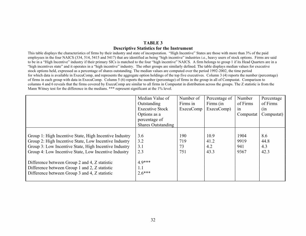
TABLE 3
Descriptive Statistics for the Instrument This table displays the characteristics of firms by their industry and state of incorporation. “High Incentive” States are those with more than 3% of the paid employees in the four NAICS (334, 514, 5415 and 5417) that are identified as being “high incentive” industries i.e., heavy users of stock options. Firms are said to be in a “High Incentive” industry if their primary SICs is matched to the four “high incentive” NAICS. A firm belongs to group 1 if its Head Quarters are in a “high incentives state” and it operates in a “high incentive” industry. The other groups are similarly defined. The table displays median values for executive stock options held, expressed as a percentage of shares outstanding. The median values are computed over the period 1992-2002, the time period for which data is available in ExecuComp, and represents the aggregate option holdings of the top five executives. Column 3 (4) reports the number (percentage) of firms in each group with data in ExecuComp. Column 5 (6) reports the number (percentage) of firms in the group in all of Compustat. Comparison to columns 4 and 6 reveals that the firms covered by ExecuComp are similar to all firms in Compustat in distribution across the groups. The Z statistic is from the Mann Witney test for the difference in the medians. *** represent significant at the 1% level. Median Value of
Outstanding Executive Stock Options as a percentage of Shares Outstanding
Number of Firms in ExecuComp
Percentage of Firms (in ExecuComp)
Number of Firms in Compustat
Percentage of Firms (in Compustat)
Group 1: High Incentive State, High Incentive Industry 3.6 190 10.9 1904 8.6 Group 2: High Incentive State, Low Incentive Industry 3.2 719 41.2 9919 44.8 Group 3: Low Incentive State, High Incentive Industry 3.1 73 4.2 941 4.3 Group 4: Low Incentive State, Low Incentive Industry 2.3 751 43.3 9367 42.3 Difference between Group 2 and 4, Z statistic 4.9*** Difference between Group 1 and 2, Z statistic 1.1 Difference between Group 3 and 4, Z statistic 2.6***
32
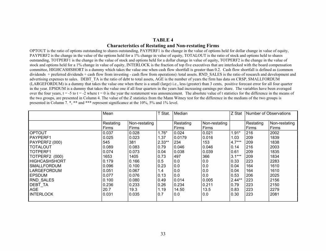
TABLE 4 Characteristics of Restating and Non-restating Firms
OPTOUT is the ratio of options outstanding to shares outstanding, PAYPERF1 is the change in the value of options held for dollar change in value of equity, PAYPERF2 is the change in the value of the options held for a 1% change in value of equity, TOTALOUT is the ratio of stock and options held to shares outstanding, TOTPERF1 is the change in the value of stock and options held for a dollar change in value of equity, TOTPERF2 is the change in the value of stock and options held for a 1% change in value of equity, INTERLOCK is the fraction of top five executives that are interlocked with the board compensation committee, HIGHCASHSHORT is a dummy which takes the value one when cash flow shortfall is greater than 0.2. Cash flow shortfall is defined as (common dividends + preferred dividends + cash flow from investing - cash flow from operations) /total assets. RND_SALES is the ratio of research and development and advertising expenses to sales. DEBT_TA is the ratio of debt to total assets, AGE is the number of years the firm has data on CRSP, SMALLFORDUM (LARGEFORDUM) is a dummy that takes the value one when there is a small (large) i.e., less (greater) than 3 cents, positive forecast error for all four quarter in the year. EPSDUM is a dummy that takes the value one if all four quarters in the years had increasing earnings per share. The variables have been averaged over the four years, t = -5 to t = -2 where t = 0 is the year the restatement was announcement. The absolute value of t statistics for the difference in the means of the two groups, are presented in Column 4. The value of the Z statistics from the Mann Witney test for the difference in the medians of the two groups is presented in Column 7. *, ** and *** represent significance at the 10%, 5% and 1% level.
Mean T Stat. Median Z Stat Number of Observations
RestatingFirms
Non-restating Firms
RestatingFirms
Non-restating Firms
RestatingFirms
Non-restating Firms
OPTOUT 0.037 0.028 1.76* 0.024 0.021 1.91* 216 2002PAYPERF1 0.025 0.023 1.37 0.0179 0.016 1.03 209 1839PAYPERF2 (000) 545 381 2.33** 234 153 4.7*** 209 1838TOTALOUT 0.089 0.083 0.79 0.046 0.046 0.14 216 2003TOTPERF1 0.074 0.073 0.04 0.038 0.039 0.61 209 1835TOTPERF2 (000) 1653 1405 0.73 497 366 3.1*** 209 1834 HIGHCASHSHORT 0.179 0.166 0.5 0.0 0.0 0.33 223 2283SMALLFORDUM 0.096 0.100 0.23 0.0 0.0 0.04 164 1610LARGEFORDUM 0.051 0.067 1.4 0.0 0.0 0.04 164 1610EPSDUM 0.077 0.076 0.13 0.0 0.0 0.53 206 2025RND_SALES 0.100 0.080 0.49 0.014 0.005 2.44** 223 2156DEBT_TA 0.236 0.233 0.26 0.234 0.211 0.79 223 2150AGE 20.7 19.3 1.19 14.50 13.5 0.83 2279223INTERLOCK 0.031 0.035 0.7 0.0 0.0 0.30 223 2081
33
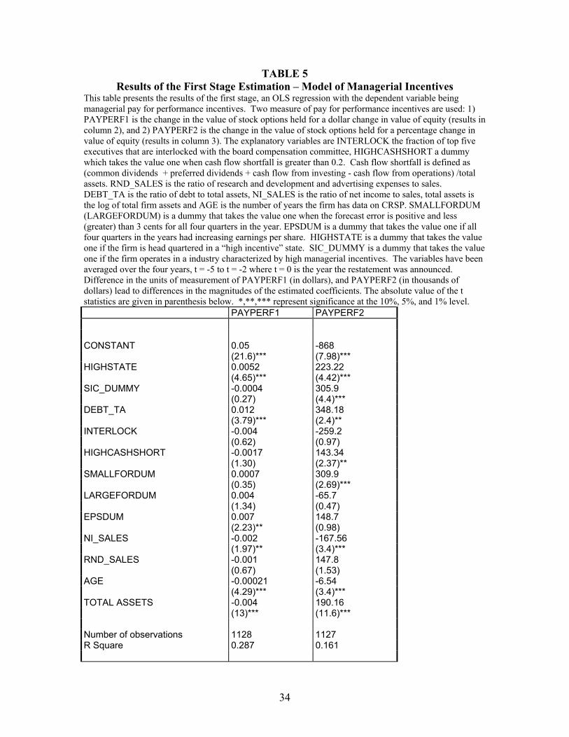
TABLE 5 Results of the First Stage Estimation – Model of Managerial Incentives
This table presents the results of the first stage, an OLS regression with the dependent variable being managerial pay for performance incentives. Two measure of pay for performance incentives are used: 1) PAYPERF1 is the change in the value of stock options held for a dollar change in value of equity (results in column 2), and 2) PAYPERF2 is the change in the value of stock options held for a percentage change in value of equity (results in column 3). The explanatory variables are INTERLOCK the fraction of top five executives that are interlocked with the board compensation committee, HIGHCASHSHORT a dummy which takes the value one when cash flow shortfall is greater than 0.2. Cash flow shortfall is defined as (common dividends + preferred dividends + cash flow from investing - cash flow from operations) /total assets. RND_SALES is the ratio of research and development and advertising expenses to sales. DEBT_TA is the ratio of debt to total assets, NI_SALES is the ratio of net income to sales, total assets is the log of total firm assets and AGE is the number of years the firm has data on CRSP. SMALLFORDUM (LARGEFORDUM) is a dummy that takes the value one when the forecast error is positive and less (greater) than 3 cents for all four quarters in the year. EPSDUM is a dummy that takes the value one if all four quarters in the years had increasing earnings per share. HIGHSTATE is a dummy that takes the value one if the firm is head quartered in a “high incentive” state. SIC_DUMMY is a dummy that takes the value one if the firm operates in a industry characterized by high managerial incentives. The variables have been averaged over the four years, t = -5 to t = -2 where t = 0 is the year the restatement was announced. Difference in the units of measurement of PAYPERF1 (in dollars), and PAYPERF2 (in thousands of dollars) lead to differences in the magnitudes of the estimated coefficients. The absolute value of the t statistics are given in parenthesis below. *,**,*** represent significance at the 10%, 5%, and 1% level. PAYPERF1 PAYPERF2 CONSTANT 0.05 -868 (21.6)*** (7.98)*** HIGHSTATE 0.0052 223.22 (4.65)*** (4.42)*** SIC_DUMMY -0.0004 305.9 (0.27) (4.4)*** DEBT_TA 0.012 348.18 (3.79)*** (2.4)** INTERLOCK -0.004 -259.2 (0.62) (0.97) HIGHCASHSHORT -0.0017 143.34 (1.30) (2.37)** SMALLFORDUM 0.0007 309.9 (0.35) (2.69)*** LARGEFORDUM 0.004 -65.7 (1.34) (0.47) EPSDUM 0.007 148.7 (2.23)** (0.98) NI_SALES -0.002 -167.56 (1.97)** (3.4)*** RND_SALES -0.001 147.8 (0.67) (1.53) AGE -0.00021 -6.54 (4.29)*** (3.4)*** TOTAL ASSETS -0.004 190.16 (13)*** (11.6)*** Number of observations 1128 1127 R Square 0.287 0.161
34

TABLE 6 Results of the Second Stage – Determinants of the Probability of Restatement
This table reports the results of the second stage probit estimation. The dependent variable is a binary variable that is equal to one if the firm announced a restatement to its financial statement from January 1997 to June 2002 and zero otherwise. Panel A reports the results with the proxy for managerial incentives being PAYPERF1 and Panel B with PAYPERF2. PAYPERF1 is the change in the value of option holdings for a dollar change in value of equity and PAYPERF2 is the change in the value of options held for a 1% change in value of equity. The explanatory variables are HIGHCASHSHORT a dummy that takes the value one when cash flow shortfall is greater than 0.2 and zero otherwise. Cash flow shortfall is defined as (common dividends + preferred dividends + cash flow from investing - cash flow from operations) /total assets. INTERLOCK is the fraction of top executives that are interlocked with the board compensation committee. RND_SALES is the ratio of research and development and advertising expenses to sales. DEBT_TA is the ratio of debt to total assets, NI_SALES is the ratio of net income to sales, TOTAL ASSETS is the log of total firm assets and AGE is the number of years the firm has data on CRSP. SMALLFORDUM (LARGEFORDUM) is a dummy that takes the value one when the forecast error is positive and less (greater) than 3 cents for all four quarters in the year. EPSDUM is a dummy that takes the value one if all four quarters in the years had increasing earnings per share. The variables have been averaged over the four years, t = -5 to t = -2 where t = 0 is the year the firm announced a restatement. RESID is the residuals from the first stage of the estimation. The t statistics and the marginal effects are displayed in the requisite columns. Difference in the units of measurement of PAYPERF1 (in dollars), and PAYPERF2 (in thousands of dollars) lead to differences in the magnitudes of the estimated coefficient. Absolute value of T statistics is displayed in Columns 3,6 and 9. *,**,*** represent significance at the 10%, 5% and 1% level. The standard errors have been adjusted for the two-step estimation. PANEL A PANEL B
ProbitCoefficients
T- Stat Marginal Effects Probit Coefficients
T- Stat Marginal Effects
Constant -4.37 2.82*** -0.851 -0.69 2.11** -0.138PAYPERF1 56.6 2.05** 11.02 PAYPERF2 0.00096 2.65*** 0.00019DEBT_TA -0.61 1.14 -0.118 0.54 1.34 0.108INTERLOCK 0.62 0.86 0.121 0.67 1.04 0.133HIGHCASHSHORT 0.097 0.55 0.019 -0.15 0.98 -0.03SMALLFORDUM -0.24 0.69 -0.0458 -0.50 1.52 -0.099LARGEFORDUM -0.42 0.99 -0.083 -0.1 0.26 -0.019EPSDUM -0.65 1.28 -0.126 -0.41 1.1 -0.083NI_SALES -0.02 0.14 -0.004 0.01 0.1 0.003RND_SALES -0.26 0.83 -0.052 -0.53 1.64 -0.106FIRM AGE 0.019 2.45** 0.0037 0.012 2.77*** 0.003TOTAL ASSETS 0.26 1.88 0.051 -0.18 2.37 -0.037RESID -53.5 1.92* -0.00087 2.36**
Number of observations 1128 1127 Maximized Likelihood Function -400.56 -398.69 Psuedo R Square 0.026 0.03 % of positive observations 11.87 11.88
35
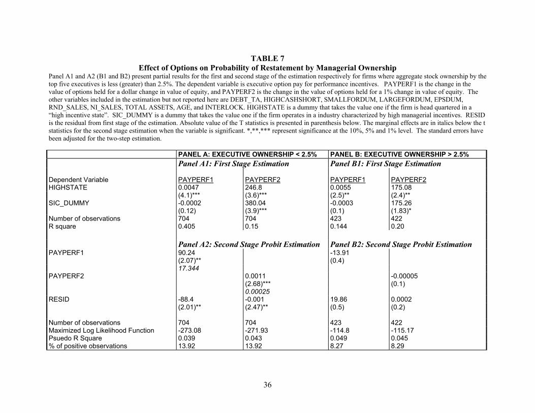
TABLE 7 Effect of Options on Probability of Restatement by Managerial Ownership
Panel A1 and A2 (B1 and B2) present partial results for the first and second stage of the estimation respectively for firms where aggregate stock ownership by the top five executives is less (greater) than 2.5%. The dependent variable is executive option pay for performance incentives. PAYPERF1 is the change in the value of options held for a dollar change in value of equity, and PAYPERF2 is the change in the value of options held for a 1% change in value of equity. The other variables included in the estimation but not reported here are DEBT_TA, HIGHCASHSHORT, SMALLFORDUM, LARGEFORDUM, EPSDUM, RND_SALES, NI_SALES, TOTAL ASSETS, AGE, and INTERLOCK. HIGHSTATE is a dummy that takes the value one if the firm is head quartered in a “high incentive state”. SIC_DUMMY is a dummy that takes the value one if the firm operates in a industry characterized by high managerial incentives. RESID is the residual from first stage of the estimation. Absolute value of the T statistics is presented in parenthesis below. The marginal effects are in italics below the t statistics for the second stage estimation when the variable is significant. *,**,*** represent significance at the 10%, 5% and 1% level. The standard errors have been adjusted for the two-step estimation. PANEL A: EXECUTIVE OWNERSHIP < 2.5% PANEL B: EXECUTIVE OWNERSHIP > 2.5% Panel A1: First Stage Estimation Panel B1: First Stage Estimation
Dependent Variable PAYPERF1 PAYPERF2 PAYPERF1 PAYPERF2 HIGHSTATE 0.0047 246.8 0.0055 175.08
(4.1)*** (3.6)*** (2.5)** (2.4)**SIC_DUMMY -0.0002 380.04 -0.0003 175.26
(0.12) (3.9)*** (0.1) (1.83)*Number of observations 704 704 423 422 R square 0.405 0.15 0.144 0.20 Panel A2: Second Stage Probit Estimation Panel B2: Second Stage Probit Estimation PAYPERF1 90.24 -13.91
(2.07)** (0.4) 17.344 PAYPERF2 0.0011 -0.00005
(2.68)*** (0.1)0.00025
RESID -88.4 -0.001 19.86 0.0002(2.01)** (2.47)** (0.5) (0.2)
Number of observations 704 704 423 422 Maximized Log Likelihood Function -273.08 -271.93 -114.8 -115.17 Psuedo R Square 0.039 0.043 0.049 0.045 % of positive observations 13.92 13.92 8.27 8.29
36
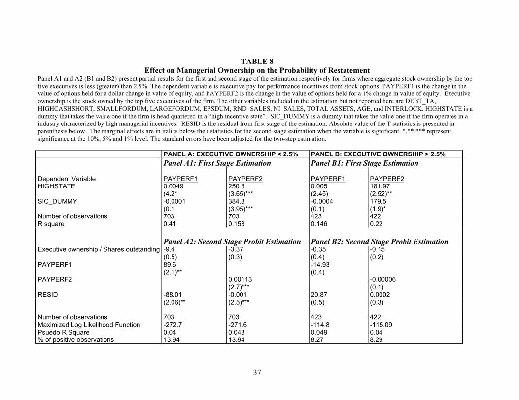
TABLE 8 Effect on Managerial Ownership on the Probability of Restatement
Panel A1 and A2 (B1 and B2) present partial results for the first and second stage of the estimation respectively for firms where aggregate stock ownership by the top five executives is less (greater) than 2.5%. The dependent variable is executive pay for performance incentives from stock options. PAYPERF1 is the change in the value of options held for a dollar change in value of equity, and PAYPERF2 is the change in the value of options held for a 1% change in value of equity. Executive ownership is the stock owned by the top five executives of the firm. The other variables included in the estimation but not reported here are DEBT_TA, HIGHCASHSHORT, SMALLFORDUM, LARGEFORDUM, EPSDUM, RND_SALES, NI_SALES, TOTAL ASSETS, AGE, and INTERLOCK. HIGHSTATE is a dummy that takes the value one if the firm is head quartered in a “high incentive state”. SIC_DUMMY is a dummy that takes the value one if the firm operates in a industry characterized by high managerial incentives. RESID is the residual from first stage of the estimation. Absolute value of the T statistics is presented in parenthesis below. The marginal effects are in italics below the t statistics for the second stage estimation when the variable is significant. *,**,*** represent significance at the 10%, 5% and 1% level. The standard errors have been adjusted for the two-step estimation. PANEL A: EXECUTIVE OWNERSHIP < 2.5% PANEL B: EXECUTIVE OWNERSHIP > 2.5% Panel A1: First Stage Estimation Panel B1: First Stage Estimation
Dependent Variable PAYPERF1 PAYPERF2 PAYPERF1 PAYPERF2 HIGHSTATE 0.0049 250.3 0.005 181.97
(4.2* (3.65)*** (2.45) (2.52)**SIC_DUMMY -0.0001 384.8 -0.0004 179.5
(0.1 (3.95)*** (0.1) (1.9)*Number of observations 703 703 423 422 R square 0.41 0.153 0.146 0.22 Panel A2: Second Stage Probit Estimation Panel B2: Second Stage Probit Estimation Executive ownership / Shares outstanding -9.4 -3.37 -0.35 -0.15 (0.5) (0.3) (0.4) (0.2)PAYPERF1 89.6 -14.93
(2.1)** (0.4)PAYPERF2 0.00113 -0.00006
(2.7)*** (0.1)RESID -88.01 -0.001 20.87 0.0002
(2.06)** (2.5)*** (0.5) (0.3)
Number of observations 703 703 423 422 Maximized Log Likelihood Function -272.7 -271.6 -114.8 -115.09 Psuedo R Square 0.04 0.043 0.049 0.04 % of positive observations 13.94 13.94 8.27 8.29
37