Do Banks Take Unusual Risks When Interest Rates are Ex-

pected to Stay Low for a Long Time?

February 21, 2017

Abstract: The financial woes that initiated the financial crisis of 2007/08 have, at least in part,been traced to excessive bank risk-taking. What induced this behavior? One explanation arepersistently low short-term interest rates during the mid-2000s. We exploit an extensive panel ofmatched Austrian banks and firms during 2000–2008 to investigate the effects of the ECB’s policyof persistently low interest rates during 2003q3-2005q3. Our analysis suggests that this periodlikely caused Austrian banks to hold risker loan portfolios than they would have in the absence ofthis policy.

JEL: E44, E52, E58, G28Keywords: monetary policy, risk-taking, financial stability

Paul Gaggl1

University of North Carolina at Charlotte

Belk College of Business

Department of Economics

9201 University City Blvd

Charlotte, NC 28223-0001

Email: pgaggl@uncc.edu

Maria Teresa Valderrama1

Oesterreichische Nationalbank

Economic Analysis Division

Otto-Wagner-Platz 3

1090 Wien, Austria

Email: maria.valderrama@oenb.at

1Any results presented in this paper reflect our personal opinion and do not represent the official stance of theOesterreichische Nationalbank (OeNB). In particular, any mistakes or misprints are entirely our responsibility. We areextremely grateful to the OeNB for providing our main dataset. In particular, we are greatly indebted to Gerhard Fiamfor compiling the raw dataset and sharing invaluable know-how with respect to the various underlying data sources.We are further grateful to Costas Arkolakis, Maya Eden, Thanasis Geromichalos, Oscar Jorda, Michal Kowalik, JohnLeahy, David Marques Ibanez, Rob Roy McGregor, Steven Ongena, Ankur Patel, Giovanni Peri, Martine Quinzii,Katheryn N. Russ, Kevin D. Salyer, Alan M. Taylor, as well as participants of the 2011 Western Economic Assosiac-tion Meetings, the 2011 European Economic Association Meetings, the 2011 Day Ahead Conference at the Swedish

1

1. IntroductionIn the wake of the financial crisis of 2007/08, there has been growing interest in the relation-

ship between the stance of monetary policy and the amount of risk taken in financial markets. Inparticular, researchers and policy makers have been discussing the possibility that a lower costof external funds may increase banks’ risk appetite and thereby cause an increase in the ex-anterisk taken in the market (e.g., Diamond and Rajan, 2012).2 Within a growing body of empiricalresearch on this so-called “risk-taking channel” of monetary policy, Jimenez et al. (2014) provideperhaps the most convincing evidence from Spain, finding that “a lower overnight interest rate in-duces lowly capitalized banks to grant more loan applications to ex ante risky firms and to commitlarger loan volumes with fewer collateral requirements to these firms, yet with a higher ex postlikelihood of default.”3

Our paper contributes to this literature along two dimensions: first, we exploit an extensive,matched firm-bank panel from Austria over the period 2000–2008, allowing us to study a lendingmarket that is dominated by predominantly locally operating banks, that is exposed to largelyexogenous monetary policy, and that experienced neither a major housing bubble nor massiveinflux of foreign capital.4 We therefore argue that this market provides an ideal setup to disentanglethe effects of monetary policy from other major factors that affected banks’ cost of external fundsin many countries around the globe (especially for real estate lending), far and foremost the UnitedStates.5

Second, we particularly focus on the effects of the ECB’s stance of policy throughout 2003q3-2005q3 on the realized ex-ante risk in banks’ loan portfolios, as opposed to the average effects ofshort term changes in the policy rate. This period was special in at least two respects: the ECBkept its main refinancing rate constant at a then unprecedented low of 2% and there was widespreadperception that policy interest rates would remain low for an extended period of time.6

Riksbank, the 2011 Graduate Student Conference at Washington University St. Louis, as well as seminar participantsat the Federal Reserve Bank of Kansas City, the ECB, and UC Davis for extremely helpful comments and suggestions.

2For similar arguments see Allen and Gale (2000) as well as broader discussions of this so-called “risk-takingchannel” of monetary policy by Borio and Zhu (2008) and Adrian and Shin (2010).

3Similar empirical studies include, for example, Delis and Kouretas (2011), Maddaloni and Peydro (2011),Altunbaset al. (2014), Buch et al. (2014a,b), Paligorova and Santos (2016), or Dell’Ariccia et al. (2016) and references therein.

4The dataset is strictly confidential and was provided by the Oesterreichische Nationalbank (OeNB, Austrian Cen-tral Bank). Access to the anonymized individual data is granted by the OeNB’s credit department on a case-by-casebasis. Contact information can be found at www.oenb.at/.

5See for example Schneider (2013), who documents stagnant Austrian housing prices during our sample period.Moreover, Redak and Weiss (2004) show that the use of credit derivatives at that time was very limited in Austria,particularly compared to other countries.

6Despite the fact that the ECB never explicilty announced to keep its main refinancing rate constant for an extendedperiod, there is evidence that markets were expecting overnight rates to stay low for an extended period. For example,

2

To accomplish this, we first estimate the average impact of changes in the cost of short-termfunds on ex-ante default risk within Austrian banks’ business loan portfolios, confirming a nowwell documented result (e.g., Jimenez et al., 2014):3 a lower cost of short term funds tends to inducemore ex-ante risk in loan portfolios throughout the period 2000-2008, on average. In a second step,we then show that this average effect is almost entirely driven by the period 2003q3-2005q3. Infact, during the periods immediately before and immediately after this episode, Austrian banks(a) showed approximately the same response to changes in the cost of short term funds and (b) areduction in the cost of funds during these periods either had no statistically significant impact or,if anything, a slightly negative impact on the amount of ex-ante risk held in loan portfolios. Takentogether, these results suggest that Austrian banks were likely taking differentially more ex-anterisk during the period of persistently low ECB policy rates.

Diamond and Rajan (2012) as well as Farhi and Tirole (2012) have recently argued that per-fectly rational bank behavior may lead to such developments. Both studies argue that anticipatedexpansive monetary policy may serve as insurance against expected future liquidity risk and thusspur excessive investment into risky long term assets. Moreover, Diamond and Rajan (2012) stressthat the optimal policy to avoid inefficient risk buildup is “[raising] rates in normal times [beyondthe level predicted by standard theory] to offset distortions from reducing rates in adverse times”.While we cannot test whether Austrian banks’ outcomes were efficient or not, we note that our re-sults are in principle consistent with these theories, as they suggest that Austrian banks were likelytaking differentially more ex-ante loan portfolio risk during the period of low and stable ECBrefinancing rates (2003q3-2005q3), compared to the remaining periods throughout 2000-2008.

Despite its policy relevance and intuitive theoretical foundations, there are several challenges toa clean identification of such a mechanism. Our empirical strategy rests on three main identifyingassumptions: first, the ECB conducts policy with the goal of stabilizing the euro area as a whole,and does not exclusively focus on the performance of individual member states. Second, we arguethat the majority of Austrian banks predominantly focus on the local business cycle. Therefore,whenever the Austrian business cycle is sufficiently “out of sync” with the overall euro area cycle,the ECB’s policy decisions are likely exogenous to Austrian banks. Under these assumptions, thedifference between a Taylor (1993) rule for Austria and the euro area should then capture largelyexogenous variation in the effective cost of short term funds for Austrian banks, since a Taylor rule

the 1-year euro overnight swap rate was on average 2.2% during 2003q3-2005q3. Based on monthly observations andNewey-West standard errors, this average was significantly below 2.25%. This implies that, up until the end of 2005,markets were expecting overnight rates to remain on average below 2.25% for at least one more year. See for exampleTaylor and Williams (2009) for an explicit formulation of the no-arbitrage argument underlying this interpretation ofovernight swap rates.

3

can be interpreted as both a measure of economic conditions and a prediction for the short-termpolicy rate. Third, we estimate the differential impact on lowly capitalized banks, as these banksface the largest moral hazard problems, and should therefore have the strongest incentive to takelarger risks in response to changes in the cost of short-term funds (Holmstrom and Tirole, 1997;Jimenez et al., 2014).7

We show that our qualitative results neither depend on a specific measure of the cycle nor dowe have to assume any particular ECB policy rule, beyond the assertion that the ECB seeks togenerally support the macroeconomy in the overall euro area. However, for comparability withprevious studies and because of its convenient dual interpretation as predicted policy rates, we usea Taylor rule—a weighted average of output and inflation gaps—as our main measure of the cycle.We also provide a variety of robustness checks and arguments for why our main results are likelynot driven by any other policy or particular event during 2003q3-2005q3, beyond the stance ofECB policy.

Our work is most closely related to Altunbas et al. (2014), Dell’Ariccia et al. (2016), as wellas Delis and Kouretas (2011), who focus on the effect of a bank’s cost of external funds on the riskcomposition of its loan portfolio. These studies utilize an array of measures for banks’ portfolio-risk—like expected default frequencies or risk-weighted assets—and postulate that changes inthese measures capture changes in banks’ risk-taking behavior. They then test whether changesin short term interest rates have an effect on these measures of risk.

What differentiates our study is a unique dataset from the Austrian business lending registryand our focus on the effect of policy interest rates that are (and are expected to remain) low andunchanged for an extended period, as opposed to the average effect of short term adjustments tothe policy rate. Maddaloni and Peydro’s (2011) work is most closely related in the latter respect.They find that the number of quarters, that short term interest rates stay below the prediction ofa Taylor rule, significantly decrease banks’ lending standards. Instead, we interpret the period2003q3-2005q3 as a “unique episode” of persistently low policy rates and ask whether bank-risk-taking in response to changes in the short-term cost of funds during this period is substantiallydifferent from other periods. Again, this episode was “special” not only because the ECB kept itsmain refinancing rate at a then unprecedented low of 2%, but also because there was widespreadperception that this policy rate would remain low and stable for an extended period.6

Finally, despite the many benefits of our dataset, we note that our analysis does not allowus to directly disentangle supply of credit from demand for credit, as we do not have access to

7The main argument is that lowly capitalized banks have the least “skin in the game” and therefore have a largerincentive to place riskier bets. This amplifies the moral hazard problems described by Diamond and Rajan (2012).

4

loan applications. However, there are several reasons for why we believe that our results arenevertheless insightful: first, our estimates for the average impact of changes in the cost of shortterm funds are fully consistent with other studies that do have access to loan applications (e.g.,Jimenez et al., 2014). Second, we find that our results are almost exclusively driven by lowlycapitalized banks. Thus, unless we believe that there were systematic changes in the compositionof Austrian credit demand precisely during 2003q3-2005q3, that were also systematically biasedtoward lowly capitalized banks, our estimates likely capture responses in credit supply, rather thancredit demand. Finally, while the goal of this paper is to study loan portfolio risk at the bank level,we also confirm that an analogous analysis of risk at the firm-bank level, which allows us to controlfor unobserved firm heterogeneity, delivers qualitatively equivalent results.

The remainder of this paper is organized as follows: Section 2 describes the details of ourempirical strategy and the dataset, while Section 3 presents the main empirical results. We offersome concluding remarks in Section 4.8

2. Empirical StrategyOur empirical strategy is a variation of that employed by Maddaloni and Peydro (2011). They

ask how changes in the short-term policy rate affect banks’ lending standards. Moreover, theyalso ask whether persistence in low short-term interest rates matters for lending standards. Todo so, they exploit arguably exogenous variation in Taylor rule residuals (relative to the observedpolicy rate) across European countries and the U.S., to estimate the impact of changes in shortterm interest rates. The main difference in our approach is that we ask a slightly different question:we treat the ECB’s stance of policy during 2003q3-2005q3 as a unique event and ask whether theaverage effect identified by Maddaloni and Peydro (2011) is predominantly driven by this particularepisode.

Another difference in our strategy is that we use the difference in Taylor rules between Austriaand the euro area to proxy plausibly exogenous variation in the short term cost of funds for Austrianbanks, rather than the residual of an Austrian Taylor rule relative to the ECB policy rate. While thedifference in the two measures is not substantial, we prefer ours for two reasons: first, it capturesthe idea that ECB policy actions are exogenous, whenever the euro area cycle is sufficiently outof sync with that in Austria. Second, we do not need to postulate that the ECB’s policy decisionsactually adhere to a Taylor rule. We simply assert that the ECB aims to stabilize the euro area

8Appendix A presents the construction of the main empirical measure of portfolio-risk (based on logit modelsfor firms’ probability of default), and detailed regression tables are provided in Appendix E. Appendix B throughAppendix D report other supplementary materials.

5

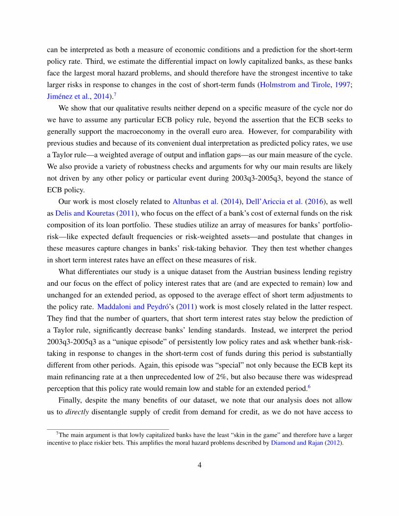
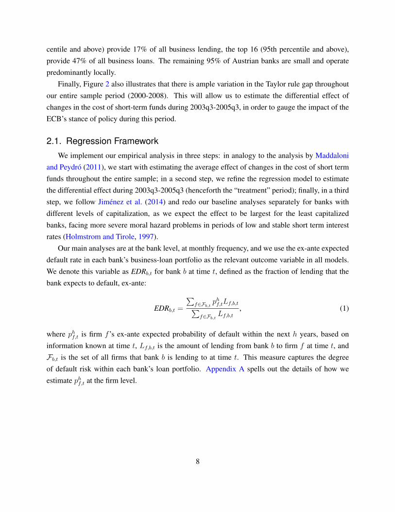
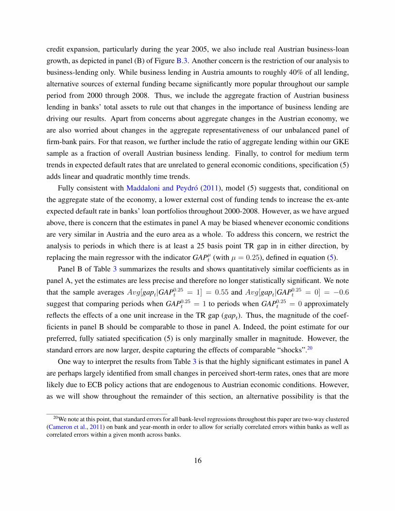
Figure 1: Taylor Rules for Austria and the Euro Area

02

46

8

AP

R

2000q3 2002q3 2004q3 2006q3 2008q3

Quarter

ECB Refi. Rate

Taylor Rule (AT Data)

Taylor Rule (EA Data)

Notes: The figure displays the a Taylor Rule for Austria (AT) and the Euro Area (EA), as utilized in equation(2). The thick solid line represents the ECB’s main refinancing rate. All three measures are expressedin annual percentage rates (APR), where the Taylor rules are interpreted as the policy rate predicted byoutput gaps and inflation. The lightly shaded rectangular area illustrates the period during which the ECBrefinancing rate was constant at 2%.

economy. While a Taylor rule—a weighted average of output and inflation gaps—is clearly ameasure of overall business conditions, the convenient dual interpretation as predicted interestrates will make it much easier to comment on the magnitude of the estimated effects.9

To illustrate the variation used in our empirical analysis, Figure 1 shows Taylor rules for Austriaand the euro area, as well as the ECB’s main refinancing rate, highlighting that the Taylor rulefor Austria deviates substantially from both the euro area Taylor rule as well as the ECB’s mainrefinancing rate.10 In stark contrast, the Taylor rule for the euro area is almost always very close tothe ECB’s refinancing rate.

The main source of independent variation used in our analysis is the difference between these

9In Appendix C we present qualitatively equivalent results for several alternative measures of economic conditions.However, the magnitudes of the effects are obviously harder to interpret.

10Our sensitivity analysis in Appendix D shows that this feature does not depend on the particular parameterizationof the Taylor Rule.

6

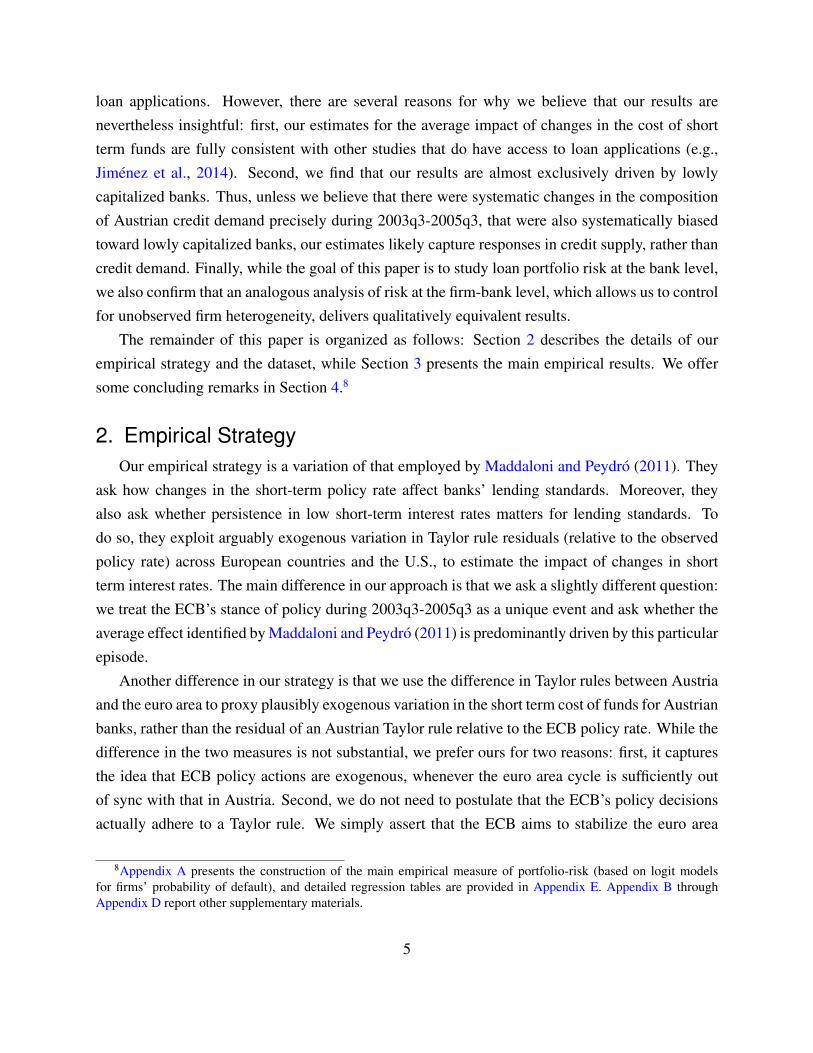
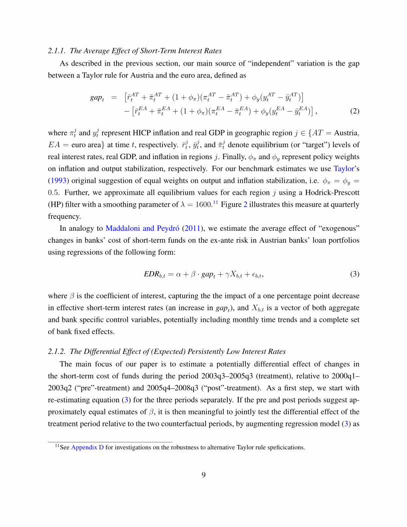
Figure 2: Economic Conditions: Austria vs. Euro Area

23

45

AP

R

−1

−.5

0.5

11.5

% G

ap

: A

ustr

ia −

Eu

ro A

rea

2000m1 2002m1 2004m1 2006m1 2008m1

Month

Gap: AT Taylor Rule − EA Taylor Rule (left)

EA Refi. Rate (right)

25bp Gap (left)

Notes: The dark shaded areas display the gap between economic conditions in Austria (AT) and the EuroArea (EA), as specified in equation (2). The dashed lines indicate when this gap is 25 basis points inabsolute value. The solid line is the ECB’s main refinancing rate, expressed as an annual percentage rate(APR). The lightly shaded rectangular area illustrates the period during which the ECB refinancing rate wasconstant at 2%.

two alternative Taylor rules, depicted in Figure 2. We note that whenever this gap is very small, thestance of policy is as if the ECB was conducting policy to specifically stabilize Austria. Given thatAustria is one of the “core” euro area countries, ECB policy decisions may thus be endogenousto Austria in such scenarios. Hence, an additional refinement to the empirical strategy used byMaddaloni and Peydro (2011) is to focus on episodes during which this gap is “sufficiently” large.Interpreting the Taylor rules as predicted nominal policy rates, a gap of 25 basis points in absolutevalue is a natural threshold, since the ECB typically changes its policy rate in increments of 25basis points. The dashed horizontal lines in Figure 2 indicates this threshold.

Under the assumptions made above, the Taylor rule gap serves as a proxy for plausibly ex-ogenous variation in the cost of funds for banks that predominantly focus on business conditionsin Austria. Thus, one important aspect of the market we study is that, indeed, the vast majorityof Austrian banks is small and operates predominantly locally. Specifically, when ranked by theamount of outstanding business loans, the top 4 out of the 316 banks in our sample (99th per-

7

centile and above) provide 17% of all business lending, the top 16 (95th percentile and above),provide 47% of all business loans. The remaining 95% of Austrian banks are small and operatepredominantly locally.

Finally, Figure 2 also illustrates that there is ample variation in the Taylor rule gap throughoutour entire sample period (2000-2008). This will allow us to estimate the differential effect ofchanges in the cost of short-term funds during 2003q3-2005q3, in order to gauge the impact of theECB’s stance of policy during this period.

2.1. Regression FrameworkWe implement our empirical analysis in three steps: in analogy to the analysis by Maddaloni

and Peydro (2011), we start with estimating the average effect of changes in the cost of short termfunds throughout the entire sample; in a second step, we refine the regression model to estimatethe differential effect during 2003q3-2005q3 (henceforth the “treatment” period); finally, in a thirdstep, we follow Jimenez et al. (2014) and redo our baseline analyses separately for banks withdifferent levels of capitalization, as we expect the effect to be largest for the least capitalizedbanks, facing more severe moral hazard problems in periods of low and stable short term interestrates (Holmstrom and Tirole, 1997).

Our main analyses are at the bank level, at monthly frequency, and we use the ex-ante expecteddefault rate in each bank’s business-loan portfolio as the relevant outcome variable in all models.We denote this variable as EDRb,t for bank b at time t, defined as the fraction of lending that thebank expects to default, ex-ante:

EDRb,t =

∑f∈Fb,t p

hf,tLf,b,t∑

f∈Fb,t Lf,b,t, (1)

where phf,t is firm f ’s ex-ante expected probability of default within the next h years, based oninformation known at time t, Lf,b,t is the amount of lending from bank b to firm f at time t, andFb,t is the set of all firms that bank b is lending to at time t. This measure captures the degreeof default risk within each bank’s loan portfolio. Appendix A spells out the details of how weestimate phf,t at the firm level.

8

2.1.1. The Average Effect of Short-Term Interest Rates

As described in the previous section, our main source of “independent” variation is the gapbetween a Taylor rule for Austria and the euro area, defined as

gapt =[rATt + πATt + (1 + φπ)(πATt − πATt ) + φy(y

ATt − yATt )

]−[rEAt + πEAt + (1 + φπ)(πEAt − πEAt ) + φy(y

EAt − yEAt )

], (2)

where πjt and yjt represent HICP inflation and real GDP in geographic region j ∈ {AT = Austria,EA = euro area} at time t, respectively. rjt , y

jt , and πjt denote equilibrium (or “target”) levels of

real interest rates, real GDP, and inflation in regions j. Finally, φπ and φy represent policy weightson inflation and output stabilization, respectively. For our benchmark estimates we use Taylor’s(1993) original suggestion of equal weights on output and inflation stabilization, i.e. φπ = φy =

0.5. Further, we approximate all equilibrium values for each region j using a Hodrick-Prescott(HP) filter with a smoothing parameter of λ = 1600.11 Figure 2 illustrates this measure at quarterlyfrequency.

In analogy to Maddaloni and Peydro (2011), we estimate the average effect of “exogenous”changes in banks’ cost of short-term funds on the ex-ante risk in Austrian banks’ loan portfoliosusing regressions of the following form:

EDRb,t = α + β · gapt + γXb,t + εb,t, (3)

where β is the coefficient of interest, capturing the the impact of a one percentage point decreasein effective short-term interest rates (an increase in gapt), and Xb,t is a vector of both aggregateand bank specific control variables, potentially including monthly time trends and a complete setof bank fixed effects.

2.1.2. The Differential Effect of (Expected) Persistently Low Interest Rates

The main focus of our paper is to estimate a potentially differential effect of changes inthe short-term cost of funds during the period 2003q3–2005q3 (treatment), relative to 2000q1–2003q2 (“pre”-treatment) and 2005q4–2008q3 (“post”-treatment). As a first step, we start withre-estimating equation (3) for the three periods separately. If the pre and post periods suggest ap-proximately equal estimates of β, it is then meaningful to jointly test the differential effect of thetreatment period relative to the two counterfactual periods, by augmenting regression model (3) as

11See Appendix D for investigations on the robustness to alternative Taylor rule speficications.

9

follows:

EDRb,t = α0 + α1TREAT t + α2 · gapt + β [gapt × TREAT t] + γXb,t + εb,t, (4)

where TREAT t is an indicator variable for the treatment period, and again, β is the coefficient ofinterest, now capturing the differential impact of a one percentage point decrease in effective short-term interest rates during the treatment period, relative to the two control periods. Put differently,it measures whether Austrian banks reacted more/less strongly to perceived changes in the costof short-term funding, during a period when the ECB kept the policy rate fixed and at a thenunprecedented low.

Due to the potential endogeneity concerns discussed in the previous section, we propose anadditional refinement to our baseline estimates, by focusing explicitly on periods during which theTaylor rule gap was “sufficiently” large. To do so, we define an additional indicator variable:

GAPµt =

{1 if gapt ≥ µ

0 if gapt ≤ −µ, (5)

isolating periods during which gapt is at least µ in either direction. Thus, conditional on a particularthreshold level µ, a modified version of regression model (4) is then

EDRb,t = αµ0 + αµ1TREAT t + αµ2GAPµt + βµ [TREAT t × GAPµt ] + γµ′Xb,t + εµb,t, (6)

where βµ is the coefficient of interest. We will illustrate in Section 3, that the interpretation ofthe estimated coefficient within our baseline analysis (with µ = 0.25) will again (approximately)correspond to the differential effect of a one percentage point decrease in the short term rate duringthe treatment period, relative to the two counterfactual periods.

2.1.3. The Differential Effect of Capitalization

Finally, we make use of the cross-sectional dimension in our dataset and investigate the impactof capitalization on the effects identified above. Based on theoretical arguments by Holmstrom andTirole (1997), Jimenez et al. (2014) make the case that due to both moral hazard and search foryield considerations, lowly capitalized banks should have a larger incentive to take on more riskin response to low interest rates than well capitalized banks. Thus, if the effects identified by theanalyses described above are driven by the same mechanism envisioned by Jimenez et al. (2014),then we should expect to see a significantly larger effect for lowly capitalized banks. To assessthis hypothesis, we simply run regressions (6) separately for banks with low, medium, and high

10

capitalization.

2.2. The DatasetOur empirical analysis draws on four main data sources. First, in order to assess individual

borrowers’ creditworthiness, we utilize annual balance sheets and income statements from an un-balanced panel of 8,653 Austrian firms over the years 1993 to 2009. This data is collected by theAustrian National Bank (OeNB) in the course of its refinancing activities and is stored in a balancesheet register (BILA). The dataset also records various auxiliary characteristics, such as the firms’age, legal form, industry classification, and the number of employees. Furthermore, we observewhether a firm went bankrupt and, if so, on which date it filed for bankruptcy protection. Oursample records a total of 533 bankruptcies, which we employ as a proxy for the event of default.

Table 1 displays summary statistics of the firm-level characteristics utilized in this study. Onecan see that our sample consists of relatively large business whose total assets range from 5 millionto 20 billion euros. Further, 72% of the firms in the sample are limited liability companies (GmbH)and 36% operate in the manufacturing sector. On average, firms’ liabilities amount to 66% of totalassets while bank-liabilities make up 26% of total assets.

Another variable of key importance for our analysis is the ratio of interest expenditure to “grossdebt”.12 We interpret this ratio as a proxy for an average firm-level interest rate on firms’ debt. Inthat sense, Austrian businesses in our sample, on average (over time and across different types ofdebt), paid a real interest rate of 2.9% during our sample period.13

In addition to annual firm specific information, the OeNB collects monthly data on individ-ual loans between Austrian firms and banks in its central credit register (GKE).14 The sampleincludes the stocks of credit by Austrian banks to Austrian firms whose total liabilities to Aus-trian banks exceed EUR 350,000, recorded at monthly frequency. We have access to a matchedBILA-GKE sample for the years 2000 through 2009 which covers 316 Austrian banks and 6,815firms whose detailed characteristics are also recorded in BILA. Table 2 reports summary statistics

12We define “gross debt” as liabilities net of long term reserves as well as provisions for pensions and other socialtransfers.

13In order to reduce the impact of measurement error on our results we drop “implausible” observations, such asnegative values for total assets, entries where detailed balance sheet positions don’t correctly sum up to reported ag-gregates, etc. Further, we identify observations that exceed five times the distance between the 5th and 95th percentileof the cross-sectional distribution in either direction as statistical outliers. We run our empirical analyses with andwithout the identified outliers and find no significant qualitative differences.

14Details on the data collection criteria can be found in the official standards for reporting to the central creditregister (Großkreditevidenz), which are publicly available at http://www.oenb.at/. The individual data on both firmsand banks are strictly confidential. Access to the anonymized individual data, as employed in this study, is granted bythe OeNB’s credit department on a case-by-case basis. Contact information can be found at www.oenb.at/.

11

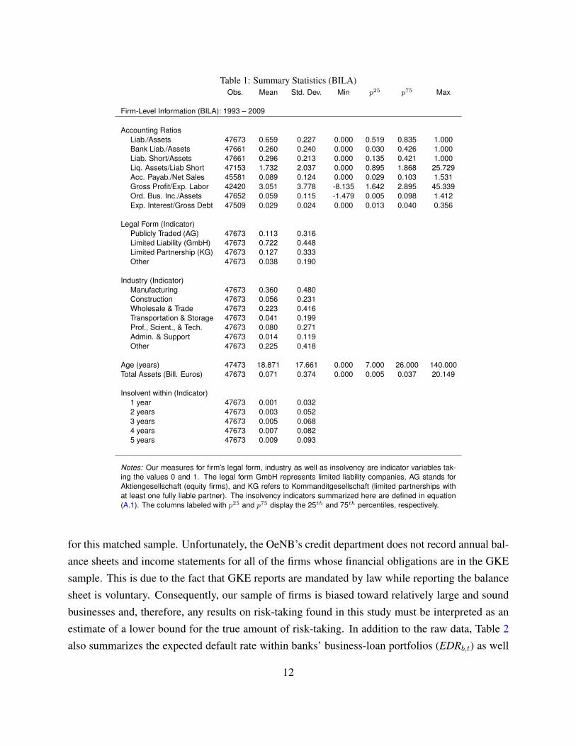
Table 1: Summary Statistics (BILA)Obs. Mean Std. Dev. Min p25 p75 Max

Firm-Level Information (BILA): 1993 – 2009

Accounting RatiosLiab./Assets 47673 0.659 0.227 0.000 0.519 0.835 1.000Bank Liab./Assets 47661 0.260 0.240 0.000 0.030 0.426 1.000Liab. Short/Assets 47661 0.296 0.213 0.000 0.135 0.421 1.000Liq. Assets/Liab Short 47153 1.732 2.037 0.000 0.895 1.868 25.729Acc. Payab./Net Sales 45581 0.089 0.124 0.000 0.029 0.103 1.531Gross Profit/Exp. Labor 42420 3.051 3.778 -8.135 1.642 2.895 45.339Ord. Bus. Inc./Assets 47652 0.059 0.115 -1.479 0.005 0.098 1.412Exp. Interest/Gross Debt 47509 0.029 0.024 0.000 0.013 0.040 0.356

Legal Form (Indicator)Publicly Traded (AG) 47673 0.113 0.316Limited Liability (GmbH) 47673 0.722 0.448Limited Partnership (KG) 47673 0.127 0.333Other 47673 0.038 0.190

Industry (Indicator)Manufacturing 47673 0.360 0.480Construction 47673 0.056 0.231Wholesale & Trade 47673 0.223 0.416Transportation & Storage 47673 0.041 0.199Prof., Scient., & Tech. 47673 0.080 0.271Admin. & Support 47673 0.014 0.119Other 47673 0.225 0.418

Age (years) 47473 18.871 17.661 0.000 7.000 26.000 140.000Total Assets (Bill. Euros) 47673 0.071 0.374 0.000 0.005 0.037 20.149

Insolvent within (Indicator)1 year 47673 0.001 0.0322 years 47673 0.003 0.0523 years 47673 0.005 0.0684 years 47673 0.007 0.0825 years 47673 0.009 0.093

Notes: Our measures for firm’s legal form, industry as well as insolvency are indicator variables tak-ing the values 0 and 1. The legal form GmbH represents limited liability companies, AG stands forAktiengesellschaft (equity firms), and KG refers to Kommanditgesellschaft (limited partnerships withat least one fully liable partner). The insolvency indicators summarized here are defined in equation(A.1). The columns labeled with p25 and p75 display the 25th and 75th percentiles, respectively.

for this matched sample. Unfortunately, the OeNB’s credit department does not record annual bal-ance sheets and income statements for all of the firms whose financial obligations are in the GKEsample. This is due to the fact that GKE reports are mandated by law while reporting the balancesheet is voluntary. Consequently, our sample of firms is biased toward relatively large and soundbusinesses and, therefore, any results on risk-taking found in this study must be interpreted as anestimate of a lower bound for the true amount of risk-taking. In addition to the raw data, Table 2also summarizes the expected default rate within banks’ business-loan portfolios (EDRb,t) as well

12

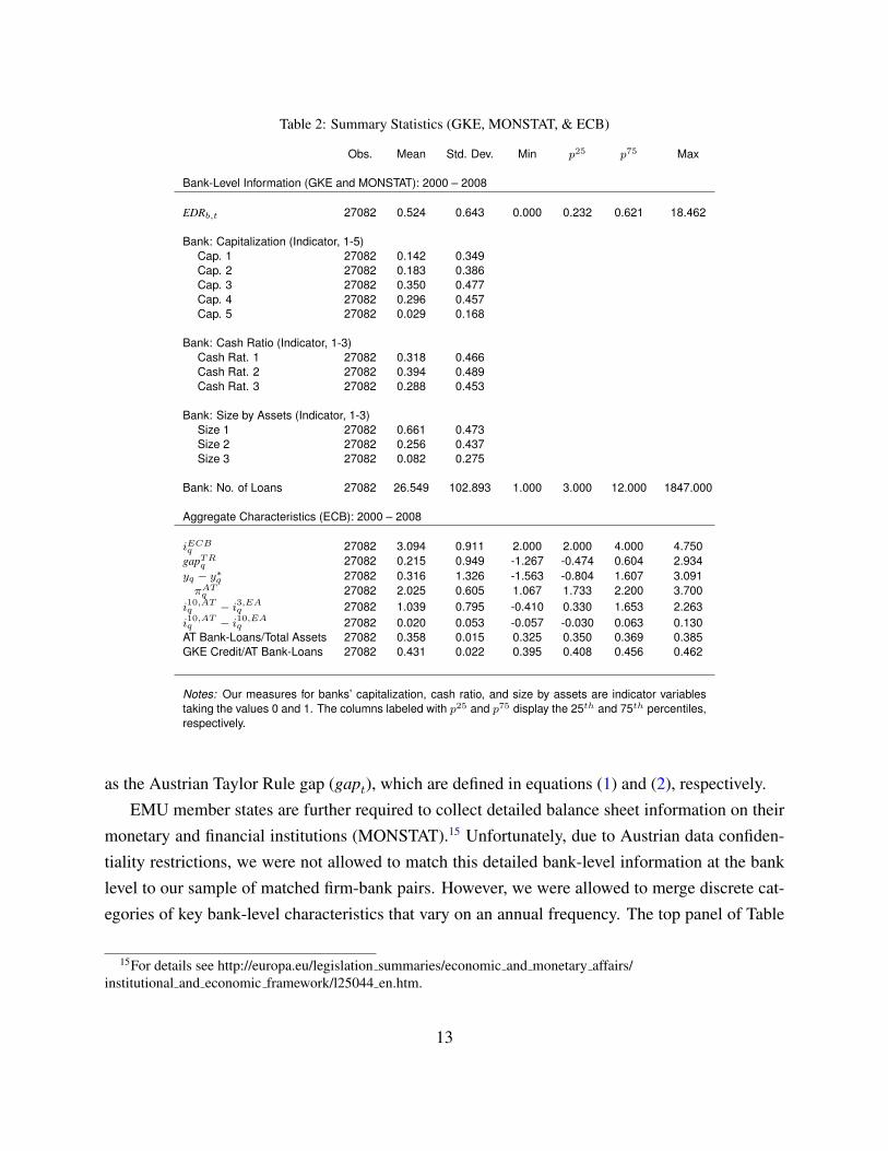
Table 2: Summary Statistics (GKE, MONSTAT, & ECB)

Obs. Mean Std. Dev. Min p25 p75 Max

Bank-Level Information (GKE and MONSTAT): 2000 – 2008

EDRb,t 27082 0.524 0.643 0.000 0.232 0.621 18.462

Bank: Capitalization (Indicator, 1-5)Cap. 1 27082 0.142 0.349Cap. 2 27082 0.183 0.386Cap. 3 27082 0.350 0.477Cap. 4 27082 0.296 0.457Cap. 5 27082 0.029 0.168

Bank: Cash Ratio (Indicator, 1-3)Cash Rat. 1 27082 0.318 0.466Cash Rat. 2 27082 0.394 0.489Cash Rat. 3 27082 0.288 0.453

Bank: Size by Assets (Indicator, 1-3)Size 1 27082 0.661 0.473Size 2 27082 0.256 0.437Size 3 27082 0.082 0.275

Bank: No. of Loans 27082 26.549 102.893 1.000 3.000 12.000 1847.000

Aggregate Characteristics (ECB): 2000 – 2008

iECBq 27082 3.094 0.911 2.000 2.000 4.000 4.750gapTRq 27082 0.215 0.949 -1.267 -0.474 0.604 2.934yq − y∗q 27082 0.316 1.326 -1.563 -0.804 1.607 3.091πATq 27082 2.025 0.605 1.067 1.733 2.200 3.700

i10,ATq − i3,EAq 27082 1.039 0.795 -0.410 0.330 1.653 2.263i10,ATq − i10,EAq 27082 0.020 0.053 -0.057 -0.030 0.063 0.130AT Bank-Loans/Total Assets 27082 0.358 0.015 0.325 0.350 0.369 0.385GKE Credit/AT Bank-Loans 27082 0.431 0.022 0.395 0.408 0.456 0.462

Notes: Our measures for banks’ capitalization, cash ratio, and size by assets are indicator variablestaking the values 0 and 1. The columns labeled with p25 and p75 display the 25th and 75th percentiles,respectively.

as the Austrian Taylor Rule gap (gapt), which are defined in equations (1) and (2), respectively.EMU member states are further required to collect detailed balance sheet information on their

monetary and financial institutions (MONSTAT).15 Unfortunately, due to Austrian data confiden-tiality restrictions, we were not allowed to match this detailed bank-level information at the banklevel to our sample of matched firm-bank pairs. However, we were allowed to merge discrete cat-egories of key bank-level characteristics that vary on an annual frequency. The top panel of Table

15For details see http://europa.eu/legislation summaries/economic and monetary affairs/institutional and economic framework/l25044 en.htm.

13

2 illustrates our measures for banks’ capitalization, liquidity, and size for the matched BILA-GKEsample.16

Finally, all aggregate data are drawn from the ECB’s statistical data warehouse.17 The bottompanel of Table 2 reports summary statistics on these aggregate variables. An important statistic forthe purpose of this study is the average proportion of business loans within banks’ balance sheets,which was 36%, on average, and was ranging between 33% and 39% between 2000 and 2008.

3. Empirical ResultsAs a baseline, we begin our empirical analysis with estimates based on regression model (3),

which are summarized in Table 3.18 Panel A effectively confirms the results by Maddaloni andPeydro (2011) for the case of Austrian business lending, suggesting that lower perceived short-term interest rates induce significantly higher expected default rates throughout 2000-2008, onaverage. While Maddaloni and Peydro (2011) specifically focus on lending standards, their resultson weakened lending standards are fully consistent with our finding of increased expected defaultrates. These baseline results are also consistent with a host of other studies that estimate theeffect of changes in short term interest rates on various measures of bank-risk (e.g., Jimenez et al.,2014).19

Column (1) of Table 3 illustrates the unconditional relationship between ex-ante expected de-fault rates at the bank level and the Taylor rule gap (TR gap) described in Section 2. As discussedin Section 2, a rise in this gap captures a perceived decrease in the short term cost of externalfunds from the perspective of Austrian banks. Columns (2) - (5) consecutively add bank-level andaggregate control variables, a full set of bank fixed effects, as well as linear and quadratic timetrends. Specifically, to control for bank-level heterogeneity, column (2) includes control variablesfor banks’ capitalization, cash ratio, and size by total assets. On top of that, we add a complete setof bank fixed effects in column (3), in order to absorb any additional time-invariant, unobservedbank heterogeneity. These bank-level control variables in part capture the effects of changes in fi-nancial regulation that were going on during this period—first and foremost the structural changesdue to (the preparation for) the Basel II accord, which became legally binding in Austria as of

16The matching of the two datasets was conducted by the OeNB’s credit department and the matched version wasdelivered to us in completely anonymized form.

17See http://sdw.ecb.europa.eu/.18Throughout the paper we show summary tables reporting only the key coefficients of interest but we provide

detailed tables with all coefficient estimates in Appendix E.19For other examples see Delis and Kouretas (2011),Altunbas et al. (2014), Buch et al. (2014a,b), Paligorova and

Santos (2016),Dell’Ariccia et al. (2016).

14

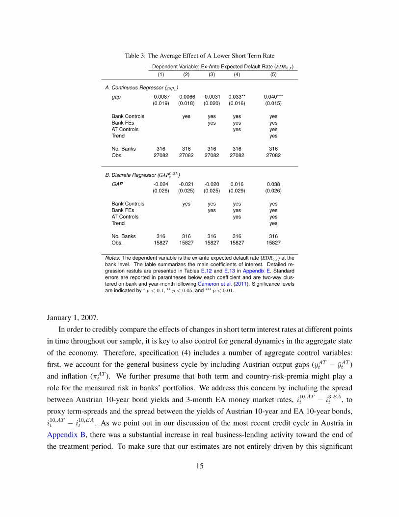
Table 3: The Average Effect of A Lower Short Term Rate

Dependent Variable: Ex-Ante Expected Default Rate (EDRb,t)(1) (2) (3) (4) (5)

A. Continuous Regressor (gapt)

gap -0.0087 -0.0066 -0.0031 0.033** 0.040***(0.019) (0.018) (0.020) (0.016) (0.015)

Bank Controls yes yes yes yesBank FEs yes yes yesAT Controls yes yesTrend yes

No. Banks 316 316 316 316 316Obs. 27082 27082 27082 27082 27082

B. Discrete Regressor (GAP0.25t )

GAP -0.024 -0.021 -0.020 0.016 0.038(0.026) (0.025) (0.025) (0.029) (0.026)

Bank Controls yes yes yes yesBank FEs yes yes yesAT Controls yes yesTrend yes

No. Banks 316 316 316 316 316Obs. 15827 15827 15827 15827 15827

Notes: The dependent variable is the ex-ante expected default rate (EDRb,t) at thebank level. The table summarizes the main coefficients of interest. Detailed re-gression restuls are presented in Tables E.12 and E.13 in Appendix E. Standarderrors are reported in parantheses below each coefficient and are two-way clus-tered on bank and year-month following Cameron et al. (2011). Significance levelsare indicated by * p < 0.1, ** p < 0.05, and *** p < 0.01.

January 1, 2007.In order to credibly compare the effects of changes in short term interest rates at different points

in time throughout our sample, it is key to also control for general dynamics in the aggregate stateof the economy. Therefore, specification (4) includes a number of aggregate control variables:first, we account for the general business cycle by including Austrian output gaps (yATt − yATt )and inflation (πATt ). We further presume that both term and country-risk-premia might play arole for the measured risk in banks’ portfolios. We address this concern by including the spreadbetween Austrian 10-year bond yields and 3-month EA money market rates, i10,ATt − i3,EAt , toproxy term-spreads and the spread between the yields of Austrian 10-year and EA 10-year bonds,i10,ATt − i10,EAt . As we point out in our discussion of the most recent credit cycle in Austria inAppendix B, there was a substantial increase in real business-lending activity toward the end ofthe treatment period. To make sure that our estimates are not entirely driven by this significant

15

credit expansion, particularly during the year 2005, we also include real Austrian business-loangrowth, as depicted in panel (B) of Figure B.3. Another concern is the restriction of our analysis tobusiness-lending only. While business lending in Austria amounts to roughly 40% of all lending,alternative sources of external funding became significantly more popular throughout our sampleperiod from 2000 through 2008. Thus, we include the aggregate fraction of Austrian businesslending in banks’ total assets to rule out that changes in the importance of business lending aredriving our results. Apart from concerns about aggregate changes in the Austrian economy, weare also worried about changes in the aggregate representativeness of our unbalanced panel offirm-bank pairs. For that reason, we further include the ratio of aggregate lending within our GKEsample as a fraction of overall Austrian business lending. Finally, to control for medium termtrends in expected default rates that are unrelated to general economic conditions, specification (5)adds linear and quadratic monthly time trends.

Fully consistent with Maddaloni and Peydro (2011), model (5) suggests that, conditional onthe aggregate state of the economy, a lower external cost of funding tends to increase the ex-anteexpected default rate in banks’ loan portfolios throughout 2000-2008. However, as we have arguedabove, there is concern that the estimates in panel A may be biased whenever economic conditionsare very similar in Austria and the euro area as a whole. To address this concern, we restrict theanalysis to periods in which there is at least a 25 basis point TR gap in in either direction, byreplacing the main regressor with the indicator GAPµt (with µ = 0.25), defined in equation (5).

Panel B of Table 3 summarizes the results and shows quantitatively similar coefficients as inpanel A, yet the estimates are less precise and therefore no longer statistically significant. We notethat the sample averages Avg[gapt|GAP0.25

t = 1] = 0.55 and Avg[gapt|GAP0.25t = 0] = −0.6

suggest that comparing periods when GAP0.25t = 1 to periods when GAP0.25

t = 0 approximatelyreflects the effects of a one unit increase in the TR gap (gapt). Thus, the magnitude of the coef-ficients in panel B should be comparable to those in panel A. Indeed, the point estimate for ourpreferred, fully satiated specification (5) is only marginally smaller in magnitude. However, thestandard errors are now larger, despite capturing the effects of comparable “shocks”.20

One way to interpret the results from Table 3 is that the highly significant estimates in panel Aare perhaps largely identified from small changes in perceived short-term rates, ones that are morelikely due to ECB policy actions that are endogenous to Austrian economic conditions. However,as we will show throughout the remainder of this section, an alternative possibility is that the

20We note at this point, that standard errors for all bank-level regressions throughout this paper are two-way clustered(Cameron et al., 2011) on bank and year-month in order to allow for serially correlated errors within banks as well ascorrelated errors within a given month across banks.

16

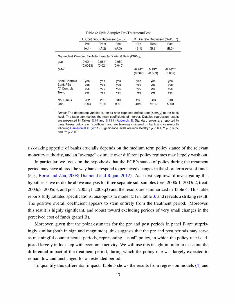
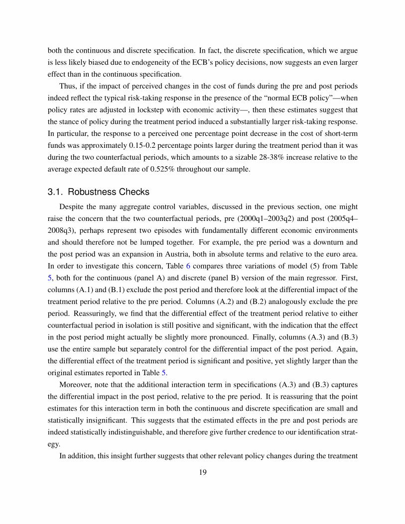
Table 4: Split Sample: Pre/Treatment/Post

A. Continuous Regressor (gapt) B. Discrete Regressor (GAP0.25t )

Pre Treat Post Pre Treat Post(A.1) (A.2) (A.3) (B.1) (B.2) (B.3)

Dependent Variable: Ex-Ante Expected Default Rate (EDRb,t)

gap -0.024** 0.064** 0.050(0.0093) (0.024) (0.040)

GAP -0.24** 0.19** -0.46***(0.087) (0.083) (0.067)

Bank Controls yes yes yes yes yes yesBank FEs yes yes yes yes yes yesAT Controls yes yes yes yes yes yesTrend yes yes yes yes yes yes

No. Banks 282 288 310 280 288 310Obs. 9903 7186 9991 4950 5616 5260

Notes: The dependent variable is the ex-ante expected default rate (EDRb,t) at the banklevel. The table summarizes the main coefficients of interest. Detailed regression restulsare presented in Tables E.14 and E.13 in Appendix E. Standard errors are reported inparantheses below each coefficient and are two-way clustered on bank and year-monthfollowing Cameron et al. (2011). Significance levels are indicated by * p < 0.1, ** p < 0.05,and *** p < 0.01.

risk-taking appetite of banks crucially depends on the medium term policy stance of the relevantmonetary authority, and an “average” estimate over different policy regimes may largely wash out.

In particular, we focus on the hypothesis that the ECB’s stance of policy during the treatmentperiod may have altered the way banks respond to perceived changes in the short term cost of funds(e.g., Borio and Zhu, 2008; Diamond and Rajan, 2012). As a first step toward investigating thishypothesis, we re-do the above analysis for three separate sub-samples (pre: 2000q1–2003q2, treat:2003q3–2005q3, and post: 2005q4–2008q3) and the results are summarized in Table 4. This tablereports fully satiated specifications, analogous to model (5) in Table 3, and reveals a striking result.The positive overall coefficient appears to stem entirely from the treatment period. Moreover,this result is highly significant, and robust toward excluding periods of very small changes in theperceived cost of funds (panel B).

Moreover, given that the point estimates for the pre and post periods in panel B are surpris-ingly similar (both in sign and magnitude), this suggests that the pre and post periods may serveas meaningful counterfactual periods, representing “usual” policy, in which the policy rate is ad-justed largely in lockstep with economic activity. We will use this insight in order to tease out thedifferential impact of the treatment period, during which the policy rate was largely expected toremain low and unchanged for an extended period.

To quantify this differential impact, Table 5 shows the results from regression models (4) and

17

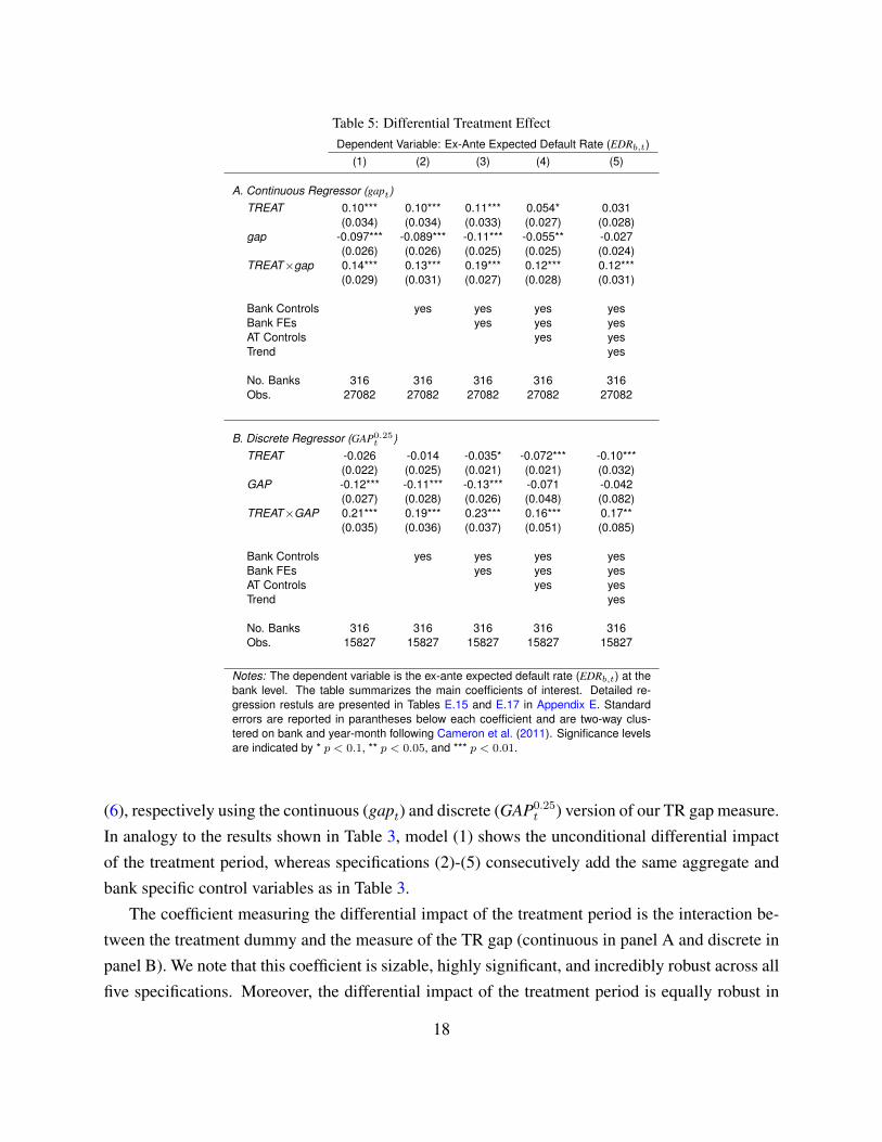
Table 5: Differential Treatment EffectDependent Variable: Ex-Ante Expected Default Rate (EDRb,t)

(1) (2) (3) (4) (5)

A. Continuous Regressor (gapt)TREAT 0.10*** 0.10*** 0.11*** 0.054* 0.031

(0.034) (0.034) (0.033) (0.027) (0.028)gap -0.097*** -0.089*** -0.11*** -0.055** -0.027

(0.026) (0.026) (0.025) (0.025) (0.024)TREAT×gap 0.14*** 0.13*** 0.19*** 0.12*** 0.12***

(0.029) (0.031) (0.027) (0.028) (0.031)

Bank Controls yes yes yes yesBank FEs yes yes yesAT Controls yes yesTrend yes

No. Banks 316 316 316 316 316Obs. 27082 27082 27082 27082 27082

B. Discrete Regressor (GAP0.25t )

TREAT -0.026 -0.014 -0.035* -0.072*** -0.10***(0.022) (0.025) (0.021) (0.021) (0.032)

GAP -0.12*** -0.11*** -0.13*** -0.071 -0.042(0.027) (0.028) (0.026) (0.048) (0.082)

TREAT×GAP 0.21*** 0.19*** 0.23*** 0.16*** 0.17**(0.035) (0.036) (0.037) (0.051) (0.085)

Bank Controls yes yes yes yesBank FEs yes yes yesAT Controls yes yesTrend yes

No. Banks 316 316 316 316 316Obs. 15827 15827 15827 15827 15827

Notes: The dependent variable is the ex-ante expected default rate (EDRb,t) at thebank level. The table summarizes the main coefficients of interest. Detailed re-gression restuls are presented in Tables E.15 and E.17 in Appendix E. Standarderrors are reported in parantheses below each coefficient and are two-way clus-tered on bank and year-month following Cameron et al. (2011). Significance levelsare indicated by * p < 0.1, ** p < 0.05, and *** p < 0.01.

(6), respectively using the continuous (gapt) and discrete (GAP0.25t ) version of our TR gap measure.

In analogy to the results shown in Table 3, model (1) shows the unconditional differential impactof the treatment period, whereas specifications (2)-(5) consecutively add the same aggregate andbank specific control variables as in Table 3.

The coefficient measuring the differential impact of the treatment period is the interaction be-tween the treatment dummy and the measure of the TR gap (continuous in panel A and discrete inpanel B). We note that this coefficient is sizable, highly significant, and incredibly robust across allfive specifications. Moreover, the differential impact of the treatment period is equally robust in

18

both the continuous and discrete specification. In fact, the discrete specification, which we argueis less likely biased due to endogeneity of the ECB’s policy decisions, now suggests an even largereffect than in the continuous specification.

Thus, if the impact of perceived changes in the cost of funds during the pre and post periodsindeed reflect the typical risk-taking response in the presence of the “normal ECB policy”—whenpolicy rates are adjusted in lockstep with economic activity—, then these estimates suggest thatthe stance of policy during the treatment period induced a substantially larger risk-taking response.In particular, the response to a perceived one percentage point decrease in the cost of short-termfunds was approximately 0.15-0.2 percentage points larger during the treatment period than it wasduring the two counterfactual periods, which amounts to a sizable 28-38% increase relative to theaverage expected default rate of 0.525% throughout our sample.

3.1. Robustness ChecksDespite the many aggregate control variables, discussed in the previous section, one might

raise the concern that the two counterfactual periods, pre (2000q1–2003q2) and post (2005q4–2008q3), perhaps represent two episodes with fundamentally different economic environmentsand should therefore not be lumped together. For example, the pre period was a downturn andthe post period was an expansion in Austria, both in absolute terms and relative to the euro area.In order to investigate this concern, Table 6 compares three variations of model (5) from Table5, both for the continuous (panel A) and discrete (panel B) version of the main regressor. First,columns (A.1) and (B.1) exclude the post period and therefore look at the differential impact of thetreatment period relative to the pre period. Columns (A.2) and (B.2) analogously exclude the preperiod. Reassuringly, we find that the differential effect of the treatment period relative to eithercounterfactual period in isolation is still positive and significant, with the indication that the effectin the post period might actually be slightly more pronounced. Finally, columns (A.3) and (B.3)use the entire sample but separately control for the differential impact of the post period. Again,the differential effect of the treatment period is significant and positive, yet slightly larger than theoriginal estimates reported in Table 5.

Moreover, note that the additional interaction term in specifications (A.3) and (B.3) capturesthe differential impact in the post period, relative to the pre period. It is reassuring that the pointestimates for this interaction term in both the continuous and discrete specification are small andstatistically insignificant. This suggests that the estimated effects in the pre and post periods areindeed statistically indistinguishable, and therefore give further credence to our identification strat-egy.

In addition, this insight further suggests that other relevant policy changes during the treatment

19

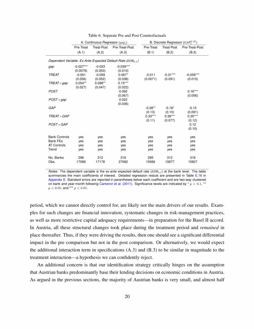
Table 6: Separate Pre and Post Counterfactuals

A. Continuous Regressor (gapt) B. Discrete Regressor (GAP0.25t )

Pre-Treat Treat-Post Pre-Treat-Post Pre-Treat Treat-Post Pre-Treat-Post(A.1) (A.2) (A.3) (B.1) (B.2) (B.3)

Dependent Variable: Ex-Ante Expected Default Rate (EDRb,t)

gap -0.027*** -0.023 -0.039***(0.0079) (0.053) (0.010)

TREAT -0.051 -0.059 0.067* -0.011 -0.31*** -0.059***(0.056) (0.052) (0.038) (0.0071) (0.091) (0.015)

TREAT×gap 0.054** 0.098** 0.15***(0.027) (0.047) (0.022)

POST 0.092 0.16***(0.067) (0.056)

POST×gap 0.022(0.036)

GAP -0.28** -0.18* -0.15(0.13) (0.10) (0.091)

TREAT×GAP 0.33*** 0.38*** 0.35***(0.11) (0.077) (0.12)

POST×GAP 0.12(0.10)

Bank Controls yes yes yes yes yes yesBank FEs yes yes yes yes yes yesAT Controls yes yes yes yes yes yesTrend yes yes yes yes yes yes

No. Banks 296 312 316 295 312 316Obs. 17089 17178 27082 10566 10877 15827

Notes: The dependent variable is the ex-ante expected default rate (EDRb,t) at the bank level. The tablesummarizes the main coefficients of interest. Detailed regression restuls are presented in Table E.16 inAppendix E. Standard errors are reported in parantheses below each coefficient and are two-way clusteredon bank and year-month following Cameron et al. (2011). Significance levels are indicated by * p < 0.1, **p < 0.05, and *** p < 0.01.

period, which we cannot directly control for, are likely not the main drivers of our results. Exam-ples for such changes are financial innovation, systematic changes in risk-management practices,as well as more restrictive capital adequacy requirements—in preparation for the Basel II accord.In Austria, all these structural changes took place during the treatment period and remained inplace thereafter. Thus, if they were driving the results, then one should see a significant differentialimpact in the pre comparison but not in the post comparison. Or alternatively, we would expectthe additional interaction term in specifications (A.3) and (B.3) to be similar in magnitude to thetreatment interaction—a hypothesis we can confidently reject.

An additional concern is that our identification strategy critically hinges on the assumptionthat Austrian banks predominantly base their lending decisions on economic conditions in Austria.As argued in the previous sections, the majority of Austrian banks is very small, and almost half

20

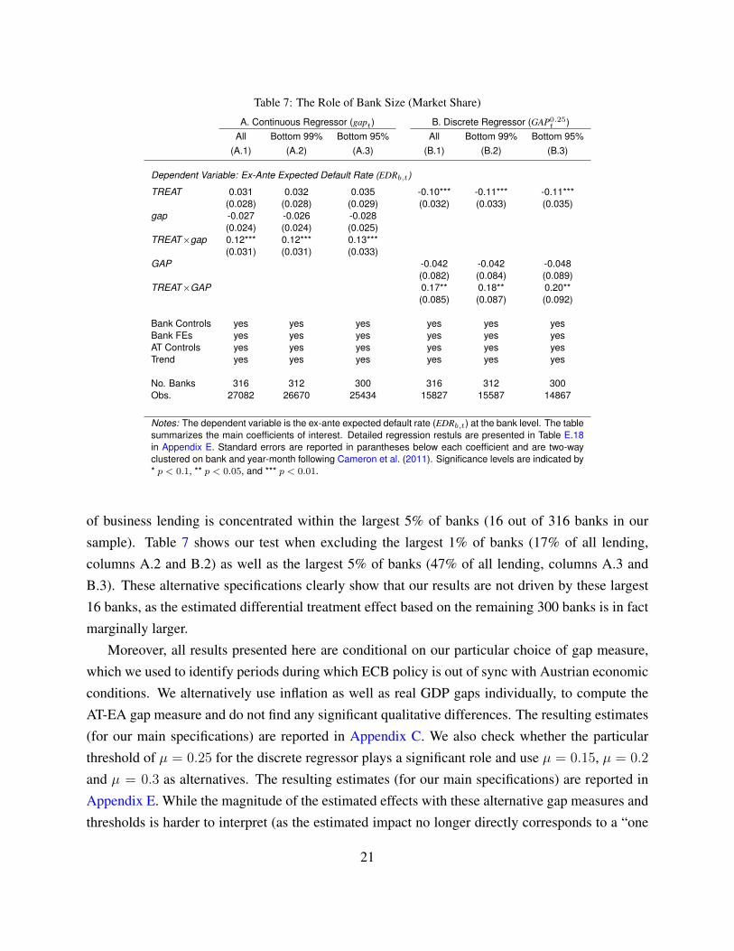
Table 7: The Role of Bank Size (Market Share)

A. Continuous Regressor (gapt) B. Discrete Regressor (GAP0.25t )

All Bottom 99% Bottom 95% All Bottom 99% Bottom 95%(A.1) (A.2) (A.3) (B.1) (B.2) (B.3)

Dependent Variable: Ex-Ante Expected Default Rate (EDRb,t)

TREAT 0.031 0.032 0.035 -0.10*** -0.11*** -0.11***(0.028) (0.028) (0.029) (0.032) (0.033) (0.035)

gap -0.027 -0.026 -0.028(0.024) (0.024) (0.025)

TREAT×gap 0.12*** 0.12*** 0.13***(0.031) (0.031) (0.033)

GAP -0.042 -0.042 -0.048(0.082) (0.084) (0.089)

TREAT×GAP 0.17** 0.18** 0.20**(0.085) (0.087) (0.092)

Bank Controls yes yes yes yes yes yesBank FEs yes yes yes yes yes yesAT Controls yes yes yes yes yes yesTrend yes yes yes yes yes yes

No. Banks 316 312 300 316 312 300Obs. 27082 26670 25434 15827 15587 14867

Notes: The dependent variable is the ex-ante expected default rate (EDRb,t) at the bank level. The tablesummarizes the main coefficients of interest. Detailed regression restuls are presented in Table E.18in Appendix E. Standard errors are reported in parantheses below each coefficient and are two-wayclustered on bank and year-month following Cameron et al. (2011). Significance levels are indicated by* p < 0.1, ** p < 0.05, and *** p < 0.01.

of business lending is concentrated within the largest 5% of banks (16 out of 316 banks in oursample). Table 7 shows our test when excluding the largest 1% of banks (17% of all lending,columns A.2 and B.2) as well as the largest 5% of banks (47% of all lending, columns A.3 andB.3). These alternative specifications clearly show that our results are not driven by these largest16 banks, as the estimated differential treatment effect based on the remaining 300 banks is in factmarginally larger.

Moreover, all results presented here are conditional on our particular choice of gap measure,which we used to identify periods during which ECB policy is out of sync with Austrian economicconditions. We alternatively use inflation as well as real GDP gaps individually, to compute theAT-EA gap measure and do not find any significant qualitative differences. The resulting estimates(for our main specifications) are reported in Appendix C. We also check whether the particularthreshold of µ = 0.25 for the discrete regressor plays a significant role and use µ = 0.15, µ = 0.2

and µ = 0.3 as alternatives. The resulting estimates (for our main specifications) are reported inAppendix E. While the magnitude of the estimated effects with these alternative gap measures andthresholds is harder to interpret (as the estimated impact no longer directly corresponds to a “one

21

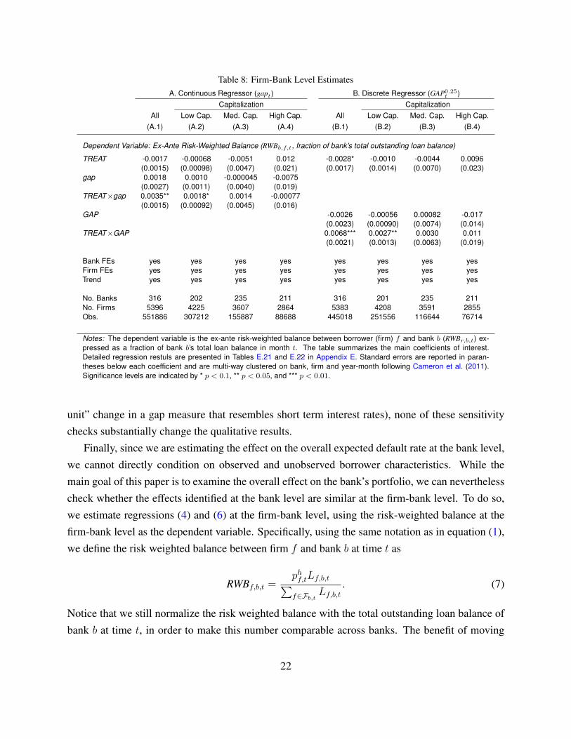
Table 8: Firm-Bank Level EstimatesA. Continuous Regressor (gapt) B. Discrete Regressor (GAP0.25

t )Capitalization Capitalization

All Low Cap. Med. Cap. High Cap. All Low Cap. Med. Cap. High Cap.(A.1) (A.2) (A.3) (A.4) (B.1) (B.2) (B.3) (B.4)

Dependent Variable: Ex-Ante Risk-Weighted Balance (RWBb,f,t, fraction of bank’s total outstanding loan balance)

TREAT -0.0017 -0.00068 -0.0051 0.012 -0.0028* -0.0010 -0.0044 0.0096(0.0015) (0.00098) (0.0047) (0.021) (0.0017) (0.0014) (0.0070) (0.023)

gap 0.0018 0.0010 -0.000045 -0.0075(0.0027) (0.0011) (0.0040) (0.019)

TREAT×gap 0.0035** 0.0018* 0.0014 -0.00077(0.0015) (0.00092) (0.0045) (0.016)

GAP -0.0026 -0.00056 0.00082 -0.017(0.0023) (0.00090) (0.0074) (0.014)

TREAT×GAP 0.0068*** 0.0027** 0.0030 0.011(0.0021) (0.0013) (0.0063) (0.019)

Bank FEs yes yes yes yes yes yes yes yesFirm FEs yes yes yes yes yes yes yes yesTrend yes yes yes yes yes yes yes yes

No. Banks 316 202 235 211 316 201 235 211No. Firms 5396 4225 3607 2864 5383 4208 3591 2855Obs. 551886 307212 155887 88688 445018 251556 116644 76714

Notes: The dependent variable is the ex-ante risk-weighted balance between borrower (firm) f and bank b (RWBr,b,t) ex-pressed as a fraction of bank b’s total loan balance in month t. The table summarizes the main coefficients of interest.Detailed regression restuls are presented in Tables E.21 and E.22 in Appendix E. Standard errors are reported in paran-theses below each coefficient and are multi-way clustered on bank, firm and year-month following Cameron et al. (2011).Significance levels are indicated by * p < 0.1, ** p < 0.05, and *** p < 0.01.

unit” change in a gap measure that resembles short term interest rates), none of these sensitivitychecks substantially change the qualitative results.

Finally, since we are estimating the effect on the overall expected default rate at the bank level,we cannot directly condition on observed and unobserved borrower characteristics. While themain goal of this paper is to examine the overall effect on the bank’s portfolio, we can neverthelesscheck whether the effects identified at the bank level are similar at the firm-bank level. To do so,we estimate regressions (4) and (6) at the firm-bank level, using the risk-weighted balance at thefirm-bank level as the dependent variable. Specifically, using the same notation as in equation (1),we define the risk weighted balance between firm f and bank b at time t as

RWBf,b,t =phf,tLf,b,t∑f∈Fb,t Lf,b,t

. (7)

Notice that we still normalize the risk weighted balance with the total outstanding loan balance ofbank b at time t, in order to make this number comparable across banks. The benefit of moving

22

the analysis to the firm-bank level is that we can now include firm fixed effects, to control for anytime invariant unobserved firm characteristics, beyond the expected default rate phf,t. We note thatwe cannot include other relevant firm characteristics as regressors, as these have been used in theestimation of phf,t, and would therefore be endogenous.

Reassuringly, columns (A.1) and (B.1) of Table 8 reveal that the firm-bank level estimatesqualitatively mirror the bank level results. However, while the bank-level estimates of the treatmentinteraction (reported in Table 5) suggest a 28-38% differential increase relative to the averageexpected default rate of 0.525%, the firm-bank level estimates indicate a slightly smaller 13.5-26.3% differential increase relative to the average risk-weighted balance at the firm-bank level of0.0258%. This suggests that our main results at the bank level are likely not exclusively driven bythe fact that we aggregate to the bank level or by unobserved firm heterogeneity.

3.2. The Role of Bank CapitalizationThe analysis in the previous sections has exclusively relied on variation over time in order to

identify the differential impact of the treatment period on expected default rates within Austrianbanks’ business loan portfolios. While we have controlled for a variety of potentially confoundingaggregate developments, it is still possible that other, unobserved, time-specific events may bebiasing our results. In order to address this concern, we conduct one final test that exploits thecross-section of our bank panel. In particular, we appeal to the argument that more pronouncedmoral hazard problems may cause lowly capitalized banks to react more strongly to the risk-takingincentive from cheap short term funds, compared to other, better capitalized banks (Holmstromand Tirole, 1997; Jimenez et al., 2014).

Within our framework, we can check this hypothesis by splitting our sample into banks withlow, medium, and high capitalization. Table 9 shows this analysis for both the continuous anddiscrete specifications, revealing that the estimated effect for lowly capitalized banks (columnsA.1 and B.1) are very close to the overall estimated effects in column (5) of Table 5. To thecontrary, the estimated treatment effect for banks with medium capitalization is about half the sizeand insignificant (columns A.2 and B.2) while it is marginally negative and insignificant for highlycapitalized banks (columns A.3 and B.3). Reassuringly, these results are mirrored by the analogousfirm-bank level estimates reported in columns (A.2)-(A.4) and (B.2)-(B.4) of Table 8.

This alternative test also suggests that our estimates are likely due to credit supply, i.e. thebank’s choice, rather than credit demand. We make this argument because we think it is unlikelythat loan applications during the treatment period were both systematically more risky and system-atically biased toward lowly capitalized banks, relative to the control periods. Thus, we concludethat the estimates shown throughout Section 3 are likely due to a risk-taking incentive for banks,

23

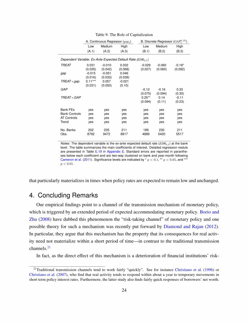
Table 9: The Role of Capitalization

A. Continuous Regressor (gapt) B. Discrete Regressor (GAP0.25t )

Low Medium High Low Medium High(A.1) (A.2) (A.3) (B.1) (B.2) (B.3)

Dependent Variable: Ex-Ante Expected Default Rate (EDRb,t)

TREAT 0.031 -0.010 0.032 -0.029 -0.060 -0.18*(0.035) (0.042) (0.068) (0.027) (0.060) (0.092)

gap -0.015 -0.051 0.046(0.016) (0.033) (0.039)

TREAT×gap 0.11*** 0.057 -0.021(0.031) (0.050) (0.10)

GAP -0.12 -0.16 0.33(0.075) (0.094) (0.30)

TREAT×GAP 0.25** 0.14 -0.11(0.094) (0.11) (0.23)

Bank FEs yes yes yes yes yes yesBank Controls yes yes yes yes yes yesAT Controls yes yes yes yes yes yesTrend yes yes yes yes yes yes

No. Banks 202 235 211 189 230 211Obs. 8792 9472 8817 4889 5420 5517

Notes: The dependent variable is the ex-ante expected default rate (EDRb,t) at the banklevel. The table summarizes the main coefficients of interest. Detailed regression restulsare presented in Table E.19 in Appendix E. Standard errors are reported in paranthe-ses below each coefficient and are two-way clustered on bank and year-month followingCameron et al. (2011). Significance levels are indicated by * p < 0.1, ** p < 0.05, and ***p < 0.01.

that particularly materializes in times when policy rates are expected to remain low and unchanged.

4. Concluding RemarksOur empirical findings point to a channel of the transmission mechanism of monetary policy,

which is triggered by an extended period of expected accommodating monetary policy. Borio andZhu (2008) have dubbed this phenomenon the “risk-taking channel” of monetary policy and onepossible theory for such a mechanism was recently put forward by Diamond and Rajan (2012).In particular, they argue that this mechanism has the property that its consequences for real activ-ity need not materialize within a short period of time—in contrast to the traditional transmissionchannels.21

In fact, as the direct effect of this mechanism is a deterioration of financial institutions’ risk-

21Traditional transmission channels tend to work fairly “quickly”. See for instance Christiano et al. (1996) orChristiano et al. (2007), who find that real activity tends to respond within about a year to temporary movements inshort term policy interest rates. Furthermore, the latter study also finds fairly quick responses of borrowers’ net worth.

24

positions, it might not result in any significant implications for the real economy under “normal”circumstances. However, in the unlikely event of a significant disruption of financial markets—like the failure of Lehman Brothers in the fall of 2008, which resulted in a global panic amonginvestors roughly 3 years after the deterioration of banks’ balance sheets had taken place—more“fragile” bank balance sheets might significantly amplify the repercussions of a “shock” to thefinancial system. Diamond and Rajan (2012) not only argue that the additional portfolio risk isinefficient but also that it increases the probability for future bailouts. The former is becauseprivate agents do not internalize the social cost of future policy interventions, while the latter isdue to increased aggregate risk exposure. While our results offer no insights regarding efficiency,they are nevertheless consistent with these theories, as they suggest differentially more risk-takingamong Austrian banks during the period of low and constant ECB policy rates.

In light of these arguments it is not surprising that Nouriel Roubini and Stephen Mihm comparethe mechanisms that lead to the 2007/2008 financial turmoil to the fault lines that eventually leadto an earthquake (Roubini and Mihm, 2010, p. 62):

[...] [T]he pressures build for many years, and when the shock finally comes, it canbe staggering. [...] The collapse revealed a frightening truth: the homes of subprimeborrowers were not the only structures standing on the proverbial fault line; countlesstowers of leverage and debt had been built there too.

Moreover, the deterioration of banks’ balance sheets during the mid 2000s was likely amplifiedby the substantial increase in the quantity of lending, that is consistent with traditional channels ofmonetary policy. This amplification is likely to have happened, as the outstanding boom in lendingactivity during the 2000s significantly increased the size of the financial sector, and hence, madeany sudden failure of this market even more detrimental to the overall economy.

Thus, the peculiar nature of this so-called “risk-taking channel” suggests that future monetarypolicy should perhaps take possible effects on financial stability more explicitly into account. Inparticular, Diamond and Rajan (2012) argue that central banks should preempt this channel and“raise rates in normal times [beyond the level predicted by standard theory] to offset distortionsfrom reducing rates in adverse times.” Farhi and Tirole (2012) make a similar case, yet they favor“macro-prudential supervision” over undirected interest rate policy.

25

ReferencesAdrian T, Shin HS. 2010. Financial Intermediaries and Monetary Economics. In Friedman BM, Woodford

M (eds.) Handbook of Monetary Economics, volume 3 of Handbook of Monetary Economics, chapter 12.Elsevier, 601–650.URL https://ideas.repec.org/h/eee/monchp/3-12.html

Allen F, Gale D. 2000. Bubbles and crises. The Economic Journal 110: 236–255. ISSN 00130133,14680297.URL http://www.jstor.org/stable/2565656

Altunbas Y, Gambacorta L, Marques-Ibanez D. 2014. Does Monetary Policy Affect Bank Risk? InternationalJournal of Central Banking 10: 95–136.URL https://ideas.repec.org/a/ijc/ijcjou/y2014q1a3.html

Bernanke BS, Gertler M. 1995. Inside the black box: The credit channel of monetary policy transmission.Journal of Economic Perspectives 9: 27–48.URL http://ideas.repec.org/a/aea/jecper/v9y1995i4p27-48.html

Borio C, Zhu H. 2008. Capital regulation, risk-taking and monetary policy: a missing link in the transmissionmechanism? BIS Working Papers 268, Bank for International Settlements.URL http://ideas.repec.org/p/bis/biswps/268.html

Buch CM, Eickmeier S, Prieto E. 2014a. In search for yield? Survey-based evidence on bank risk taking.Journal of Economic Dynamics and Control 43: 12–30.URL https://ideas.repec.org/a/eee/dyncon/v43y2014icp12-30.html

Buch CM, Eickmeier S, Prieto E. 2014b. Macroeconomic Factors and Microlevel Bank Behavior. Journal ofMoney, Credit and Banking 46: 715–751.URL https://ideas.repec.org/a/wly/jmoncb/v46y2014i4p715-751.html

Cameron AC, Gelbach JB, Miller DL. 2011. Robust Inference With Multiway Clustering. Journal of Business& Economic Statistics 29: 238–249.URL https://ideas.repec.org/a/taf/jnlbes/v29y2011i2p238-249.html

Christiano LJ, Eichenbaum M, Evans C. 1996. The effects of monetary policy shocks: Evidence from theflow of funds. The Review of Economics and Statistics 78: 16–34.URL http://ideas.repec.org/a/tpr/restat/v78y1996i1p16-34.html

Christiano LJ, Trabandt M, Walentin K. 2007. Introducing financial frictions and unemployment into a smallopen economy model. Working Paper Series 214, Sveriges Riksbank (Central Bank of Sweden).URL http://ideas.repec.org/p/hhs/rbnkwp/0214.html

Delis MD, Kouretas GP. 2011. Interest rates and bank risk-taking. Journal of Banking & Finance 35: 840–855.URL http://ideas.repec.org/a/eee/jbfina/v35y2011i4p840-855.html

26

Dell’Ariccia G, Laeven L, Suarez GA. 2016. Bank leverage and monetary policy’s risk-taking channel:Evidence from the united states. Forthcoming in The Journal of Finance .URL http://dx.doi.org/10.1111/jofi.12467

Diamond DW, Rajan RG. 2012. Illiquid banks, financial stability, and interest rate policy. Journal of PoliticalEconomy 120: 552 – 591.URL http://ideas.repec.org/a/ucp/jpolec/doi10.1086-666669.html

Farhi E, Tirole J. 2012. Collective moral hazard, maturity mismatch, and systemic bailouts. AmericanEconomic Review 102: 60–93.URL http://ideas.repec.org/a/aea/aecrev/v102y2012i1p60-93.html

Hayden E. 2003. Are credit scoring models sensitive with respect to default definitions? evidence from theaustrian market. Efma 2003 helsinki meetings, University of Vienna - Department of Business Adminis-tration.

Holmstrom B, Tirole J. 1997. Financial intermediation, loanable funds, and the real sector. The QuarterlyJournal of Economics 112: 663–91.URL http://ideas.repec.org/a/tpr/qjecon/v112y1997i3p663-91.html

Jimenez G, Ongena S, Peydro JL, Saurina J. 2014. Hazardous times for monetary policy: What do twenty-three million bank loans say about the effects of monetary policy on credit risk-taking? Econometrica 82:463–505. ISSN 1468-0262.URL http://dx.doi.org/10.3982/ECTA10104

Maddaloni A, Peydro J. 2011. Bank risk-taking, securitization, supervision, and low interest rates: Evidencefrom the euro-area and the us lending standards. Review of Financial Studies 24: 2121–2165.

Paligorova T, Santos JA. 2016. Monetary policy and bank risk-taking: Evidence from the corporate loanmarket. Journal of Financial Intermediation : –ISSN 1042-9573.URL http://www.sciencedirect.com/science/article/pii/S1042957316300626

Redak V, Weiss E. 2004. Innovative Credit Risk Transfer Instruments and Financial Stability in Austria.Financial Stability Report : 64–76.URL https://ideas.repec.org/a/onb/oenbfs/y2004i7b2.html

Roubini N, Mihm S. 2010. Crisis Economics: A Crash Course in the Future of Finance. New York: ThePenguin Press.

Schneider M. 2013. Are Recent Increases of Residential Property Prices in Vienna and Austria Justified byFundamentals? Monetary Policy & the Economy : 29–46.URL https://ideas.repec.org/a/onb/oenbmp/y2013i4b1.html

Taylor JB. 1993. Discretion versus policy rules in practice. Carnegie-Rochester Conference Series onPublic Policy 39: 195 – 214. ISSN 0167-2231.URL http://www.sciencedirect.com/science/article/B6V8D-4593CYN-V/2/

cb131b9059003dff66ea79b0830837b3

27

Taylor JB, Williams JC. 2009. A black swan in the money market. American Economic Journal: Macroeco-nomics 1: 58–83.URL http://ideas.repec.org/a/aea/aejmac/v1y2009i1p58-83.html

Woodford M. 2010. Financial intermediation and macroeconomic analysis. Journal of Economic Perspec-tives 24: 21–44.

Appendix A. An Empirical Measure of Banks’ Loan-Portfolio RiskWe use borrowers’ annual balance sheets and income statements to estimate a probability of

default (PD) for each of the firms in our sample. We proxy the event of default, using the 533bankruptcies observed within our unbalanced panel of 8,653 Austrian firms observed between1993 and 2009. More precisely, to indicate the event that a firm declares insolvency within h yearsfrom year y, we define

INShf,y =

1 if firm f declares bankruptcy

in any of the years y ∈ {y, y + 1, ..., y + h}0 otherwise

(A.1)

Further, we construct

LOf,y = γ0 + γ′1 · ARf,y + γ′2 · LFf,y + γ′3 · INDf,y + γ′4 · Zf,y, (A.2)

where ARf,y is a k1 × 1 vector of accounting ratios derived from firms’ annual balance sheetsand income statements, LFf,y is a k2 × 1 vector of dummies for the firm’s legal form, INDf,y

is a k3 × 1 vector of industry dummies, and Zf,y represents a k4 × 1 vector of additional firmspecific characteristics including the firm’s age. The vector γ = (γ0, γ

′1, ..., γ

′4)′ ∈ RK is a vector

of coefficients with K = 1+∑4

i=1 ki. The particular choice of accounting ratios in ARf,y is guidedby results in Hayden’s (2003) earlier work on predicting Austrian firms’ PDs. Thus, based on theabove definitions we estimate the logit models

phf,y∗ ≡ Pr[

˜INSh,y∗

f,y = 1∣∣∣ARf,y,LFf,y, INDf,y, Zf,y, y ≤ y∗

]=

exp(LOf,y)

1 + exp(LOf,y), (A.3)

for the years y∗ ∈ {2000, ..., 2009}, where

˜INSh,y∗

f,y =

{INShf,y if firm f declares bankruptcy before y∗ + 1

undefined otherwise.

28

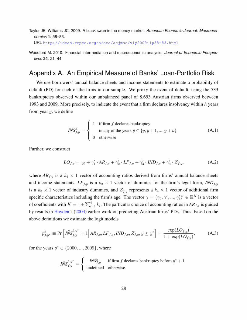
Table A.10: Logit Regressions for Predicting the Probability of Default

Dependent Variable: Insolvency within the next 3 years

Year 2000 2001 2002 2003 2004 2005 2006 2007 2008 2009

Accounting Ratios

Liab./Assets 4.392*** 3.697*** 3.683*** 3.405*** 2.966*** 3.280*** 3.390*** 3.545*** 3.619*** 3.697***(1.363) (1.172) (1.060) (1.087) (0.995) (1.007) (1.000) (0.987) (0.977) (0.980)

Bank Liab./Assets 1.469 1.753 1.735* 1.472 1.701* 1.351 1.355* 1.306* 1.281* 1.275*(1.363) (1.136) (1.022) (0.934) (0.868) (0.839) (0.823) (0.791) (0.777) (0.772)

Liab. Short/Assets 0.778 1.004 0.874 0.759 1.112 0.820 0.821 0.676 0.634 0.621(1.523) (1.273) (1.162) (1.076) (0.985) (0.942) (0.926) (0.898) (0.879) (0.874)

Liq. Assets/Liab Short 0.051 0.038 0.053 0.048 0.079* 0.070 0.068 0.056 0.052 0.055(0.093) (0.072) (0.061) (0.060) (0.046) (0.049) (0.046) (0.045) (0.044) (0.043)

Acc. Payab./Net Sales 1.988*** 1.738*** 2.136*** 2.095*** 2.084*** 2.061*** 2.058*** 1.980*** 2.015*** 2.043***(0.569) (0.551) (0.487) (0.433) (0.385) (0.372) (0.354) (0.348) (0.340) (0.336)

Gross Profit/Exp. Labor -0.322** -0.108 -0.139 -0.125 -0.126 -0.142 -0.155 -0.140 -0.149* -0.150*(0.136) (0.107) (0.117) (0.101) (0.089) (0.093) (0.097) (0.086) (0.088) (0.087)

Ord. Bus. Inc./Assets -1.906 -3.091*** -3.015*** -3.023*** -3.113*** -3.090*** -2.997*** -2.943*** -2.883*** -2.790***(1.288) (0.944) (0.839) (0.760) (0.683) (0.669) (0.639) (0.629) (0.604) (0.606)

Exp. Interest/Gross Debt 16.559*** 14.346*** 13.666*** 14.596*** 14.099*** 14.583*** 15.372*** 14.936*** 14.696*** 14.359***(3.206) (2.960) (2.901) (2.486) (2.306) (2.236) (2.035) (1.959) (1.902) (1.921)

Legal Form (relative to GmbH)

AG 0.466 0.641* 0.620* 0.623* 0.534* 0.505 0.552* 0.609* 0.635** 0.618*(0.450) (0.385) (0.365) (0.333) (0.319) (0.321) (0.322) (0.321) (0.320) (0.322)

KG 0.571* 0.485 0.520* 0.435 0.290 0.273 0.285 0.303 0.321 0.319(0.313) (0.297) (0.284) (0.279) (0.269) (0.267) (0.267) (0.267) (0.267) (0.267)

Other -0.040 -0.152 0.266 0.083 0.003 0.009 0.058 0.276 0.301 0.304(0.736) (0.731) (0.609) (0.613) (0.609) (0.609) (0.609) (0.551) (0.556) (0.554)

Industry (relative to Manufacturing)

Construction -0.121 -0.110 -0.186 -0.223 -0.170 -0.254 -0.285 -0.286 -0.302 -0.314(0.553) (0.528) (0.527) (0.513) (0.442) (0.441) (0.435) (0.429) (0.427) (0.427)

Wholesale & Trade -0.509 -0.462 -0.234 -0.264 -0.386 -0.408 -0.414 -0.423 -0.434 -0.431(0.342) (0.328) (0.303) (0.296) (0.278) (0.275) (0.273) (0.272) (0.272) (0.272)

Prof., Scient., & Tech. 0.108 -0.082 0.011 -0.141 -0.394 -0.518 -0.587 -0.721 -0.751* -0.740*(0.487) (0.476) (0.429) (0.421) (0.417) (0.424) (0.427) (0.445) (0.441) (0.438)

Admin. & Support 1.561* 1.518** 1.481** 1.306** 1.061* 0.902 0.812 0.672 0.630 0.642(0.821) (0.621) (0.625) (0.619) (0.596) (0.587) (0.584) (0.590) (0.585) (0.582)

Other 0.035 0.064 0.067 0.040 -0.112 -0.174 -0.209 -0.254 -0.290 -0.287(0.339) (0.307) (0.299) (0.285) (0.274) (0.272) (0.271) (0.270) (0.271) (0.271)

Transportation & Storage -1.102 -1.185 -1.286 -1.504 -1.585 -1.631 -1.707* -1.753* -1.751*(1.029) (1.030) (1.027) (1.019) (1.020) (1.019) (1.021) (1.021) (1.021)

Age -0.014 -0.011 -0.004 -0.025 -0.020 -0.025 -0.025 -0.025 -0.027 -0.029*(0.025) (0.024) (0.024) (0.018) (0.017) (0.016) (0.016) (0.017) (0.017) (0.017)

Age2 -0.000 -0.000 -0.000 0.000 0.000 0.000 0.000 0.000 0.000 0.000(0.000) (0.000) (0.000) (0.000) (0.000) (0.000) (0.000) (0.000) (0.000) (0.000)

Constant -8.936*** -8.775*** -8.802*** -8.327*** -8.101*** -8.101*** -8.288*** -8.427*** -8.485*** -8.540***(0.937) (0.897) (0.846) (0.796) (0.715) (0.717) (0.724) (0.726) (0.731) (0.737)

Obs. 15261 17692 19608 21794 24582 28027 32093 36294 40063 41380Model p-value 0.000 0.000 0.000 0.000 0.000 0.000 0.000 0.000 0.000 0.000AUC Ex-Ante 0.757 0.756 0.774 0.768 0.756 0.832 0.797 0.873 . .AUC Ex-Post 0.806 0.809 0.809 0.818 0.823 0.828 0.834 0.838 0.841 0.842

Notes: The table reports the maximum likelihood estimates of coefficient vector γ in equation (A.2) based on logit models (A.3).Standard errors, reported in parentheses below each coefficient estimate, are corrected for serial correlation and clustered on firm.Coefficients that are significantly different from zero are indicated with ∗∗∗ for a p-value p < 0.01, ∗∗ for p < 0.05, and ∗ for p < 0.1.The omitted legal form are limited liability companies (GmbH), AG stands for Aktiengesellschaft (equity firms), and KG refers toKommanditgesellschaft (limited partnerships with at least one fully liable partner). The omitted industry is the manufacturing sector.Ex-ante AUC values for the years 2008 through 2009 could not be computed since we observe too few bankruptcies for those yearswithin our sample of firms.

29

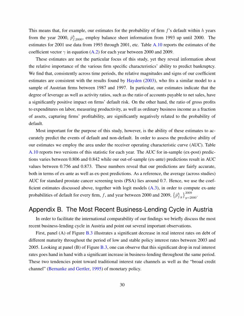
This means that, for example, our estimates for the probability of firm f ’s default within h yearsfrom the year 2000, phf,2000, employ balance sheet information from 1993 up until 2000. Theestimates for 2001 use data from 1993 through 2001, etc. Table A.10 reports the estimates of thecoefficient vector γ in equation (A.2) for each year between 2000 and 2009.

These estimates are not the particular focus of this study, yet they reveal information aboutthe relative importance of the various firm specific characteristics’ ability to predict bankruptcy.We find that, consistently across time periods, the relative magnitudes and signs of our coefficientestimates are consistent with the results found by Hayden (2003), who fits a similar model to asample of Austrian firms between 1987 and 1997. In particular, our estimates indicate that thedegree of leverage as well as activity ratios, such as the ratio of accounts payable to net sales, havea significantly positive impact on firms’ default risk. On the other hand, the ratio of gross profitsto expenditures on labor, measuring productivity, as well as ordinary business income as a fractionof assets, capturing firms’ profitability, are significantly negatively related to the probability ofdefault.

Most important for the purpose of this study, however, is the ability of these estimates to ac-curately predict the events of default and non-default. In order to assess the predictive ability ofour estimates we employ the area under the receiver operating characteristic curve (AUC). TableA.10 reports two versions of this statistic for each year. The AUC for in-sample (ex-post) predic-tions varies between 0.806 and 0.842 while our out-of-sample (ex-ante) predictions result in AUCvalues between 0.756 and 0.873. These numbers reveal that our predictions are fairly accurate,both in terms of ex-ante as well as ex-post predictions. As a reference, the average (across studies)AUC for standard prostate cancer screening tests (PSA) lies around 0.7. Hence, we use the coef-ficient estimates discussed above, together with logit models (A.3), in order to compute ex-anteprobabilities of default for every firm, f , and year between 2000 and 2009,

{phf,y}2009y=2000

.

Appendix B. The Most Recent Business-Lending Cycle in AustriaIn order to facilitate the international comparability of our findings we briefly discuss the most

recent business-lending cycle in Austria and point out several important observations.First, panel (A) of Figure B.3 illustrates a significant decrease in real interest rates on debt of

different maturity throughout the period of low and stable policy interest rates between 2003 and2005. Looking at panel (B) of Figure B.3, one can observe that this significant drop in real interestrates goes hand in hand with a significant increase in business-lending throughout the same period.These two tendencies point toward traditional interest rate channels as well as the “broad creditchannel” (Bernanke and Gertler, 1995) of monetary policy.

30

Figure B.3: The Most Recent Business-Lending Cycle in Austria (2000 - 2010)

(A) Financing Conditions (B) Aggregate Business-Lending

02

46

AP

R

1999q1 2002q1 2005q1 2008q1 2011q1

Quarter

ECB Refi. Rate AT Loan Term−Spread

AT Loan Rate (< 1 year) AT Loan Rate (> 5 years)

20

02

20

24

02

60

28

03

00

Real B

ank−

Loans to n

on−

MF

Is

01

02

03

0

Real B

ank−

Loan G

row

th (

AP

R)

1999q1 2002q1 2005q1 2008q1 2011q1

Quarter

AT Real Bank−Loan Growth

AT Real Bank−Loans to non−MFIs

Notes: Panel (A) illustrates nominal interest rates on the ECB’s main refinancing facility as well as real interest rates for Austrian (AT)bank-credit of different maturity. Real rates are computed by subtracting AT HICP inflation. Further, we report the term-spread betweenloan rates for the two reported maturities. Panel (B) depicts levels and annualized quarterly growth rates of Austrian real bank-lendingto non monetary and financial institutions (non-MFIs). A real series is constructed by dividing nominal bank-lending (in billions of Euros)by the AT GDP deflator (2005q1=100). All data are drawn from the ECB’s statistical data warehouse (http://sdw.ecb.europa.eu). Thegray areas indicate the period during which ECB refinancing rates were kept at 2%.

Second, Figure B.3 further hints at a channel recently emphasized by Woodford (2010). Heargues that a strong amplification mechanism in the transmission of monetary policy is triggeredwhenever the spread between long-term and short-term interest rates decreases. This is motivatedby the fact that investment decisions—and hence real activity—generally depend mostly on long-term rather than short-term financing conditions. One can see that the biggest spike in business-lending growth, during 2005, precisely coincides with the onset of a decline in the spread betweenloans of maturity greater than 5 years and loans with maturity less than 1 year.

Furthermore, it appears that these mechanisms were also likely to be at work at the end of 2007,in mid 2008, as well as in the year 2010. Thus, we argue that these channels are important featuresof the monetary transmission mechanism but do not seem to be phenomena that are restricted toperiods of extremely low and stable policy interest rates.

Appendix C. Alternative Measures of Economic ConditionsFigure C.4 illustrates the main thought experiment based on two alternative measures of the

cycle: HICP inflation, and the real output gap. Since these two measures do not have a natural in-terpretation in terms of interest rates, it is not obvious what an appropriate value for µ is. Choosingµ = 0.15 delivers a thought experiment that is very similar to our main specification. In fact, whenusing these two measures, the main regression results are qualitatively equivalent to those in our

31

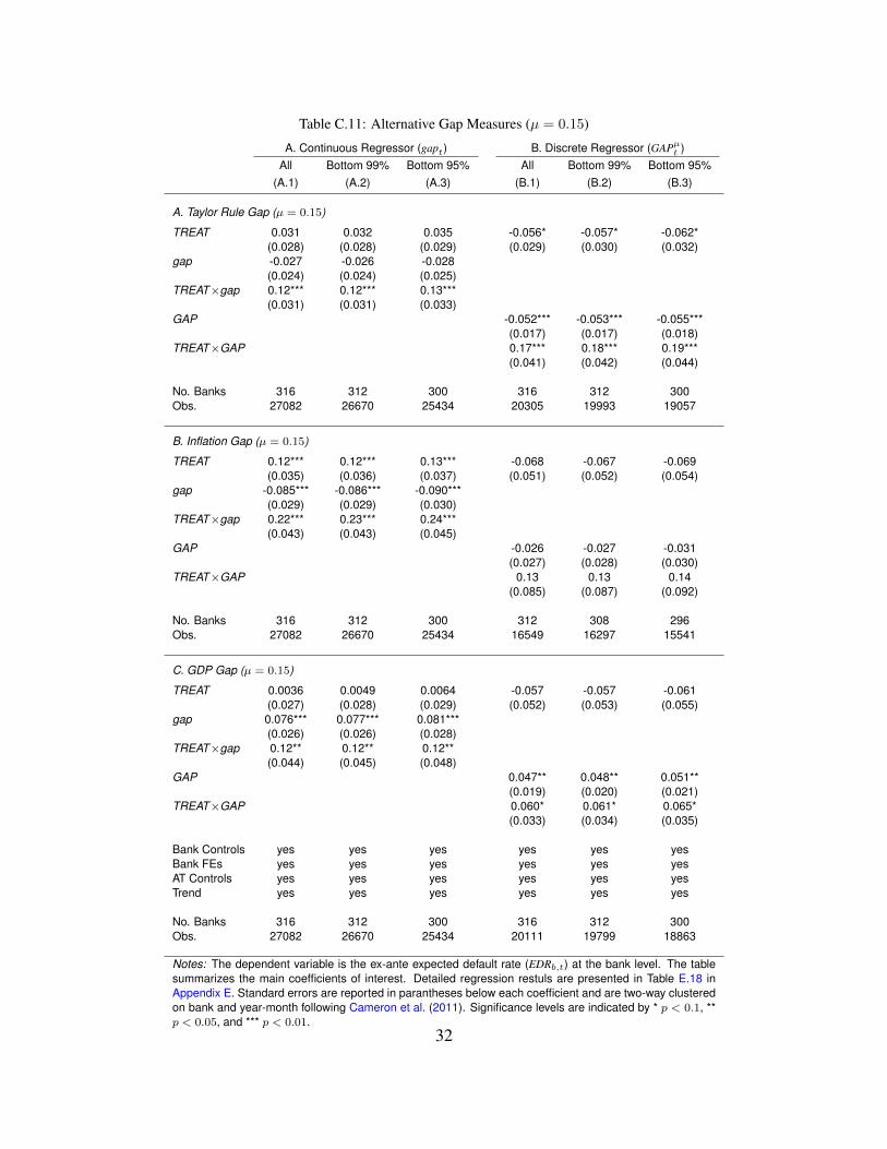
Table C.11: Alternative Gap Measures (µ = 0.15)

A. Continuous Regressor (gapt) B. Discrete Regressor (GAPµt )All Bottom 99% Bottom 95% All Bottom 99% Bottom 95%

(A.1) (A.2) (A.3) (B.1) (B.2) (B.3)

A. Taylor Rule Gap (µ = 0.15)

TREAT 0.031 0.032 0.035 -0.056* -0.057* -0.062*(0.028) (0.028) (0.029) (0.029) (0.030) (0.032)

gap -0.027 -0.026 -0.028(0.024) (0.024) (0.025)

TREAT×gap 0.12*** 0.12*** 0.13***(0.031) (0.031) (0.033)

GAP -0.052*** -0.053*** -0.055***(0.017) (0.017) (0.018)

TREAT×GAP 0.17*** 0.18*** 0.19***(0.041) (0.042) (0.044)

No. Banks 316 312 300 316 312 300Obs. 27082 26670 25434 20305 19993 19057

B. Inflation Gap (µ = 0.15)

TREAT 0.12*** 0.12*** 0.13*** -0.068 -0.067 -0.069(0.035) (0.036) (0.037) (0.051) (0.052) (0.054)

gap -0.085*** -0.086*** -0.090***(0.029) (0.029) (0.030)

TREAT×gap 0.22*** 0.23*** 0.24***(0.043) (0.043) (0.045)

GAP -0.026 -0.027 -0.031(0.027) (0.028) (0.030)

TREAT×GAP 0.13 0.13 0.14(0.085) (0.087) (0.092)

No. Banks 316 312 300 312 308 296Obs. 27082 26670 25434 16549 16297 15541

C. GDP Gap (µ = 0.15)

TREAT 0.0036 0.0049 0.0064 -0.057 -0.057 -0.061(0.027) (0.028) (0.029) (0.052) (0.053) (0.055)

gap 0.076*** 0.077*** 0.081***(0.026) (0.026) (0.028)

TREAT×gap 0.12** 0.12** 0.12**(0.044) (0.045) (0.048)

GAP 0.047** 0.048** 0.051**(0.019) (0.020) (0.021)

TREAT×GAP 0.060* 0.061* 0.065*(0.033) (0.034) (0.035)

Bank Controls yes yes yes yes yes yesBank FEs yes yes yes yes yes yesAT Controls yes yes yes yes yes yesTrend yes yes yes yes yes yes

No. Banks 316 312 300 316 312 300Obs. 27082 26670 25434 20111 19799 18863

Notes: The dependent variable is the ex-ante expected default rate (EDRb,t) at the bank level. The tablesummarizes the main coefficients of interest. Detailed regression restuls are presented in Table E.18 inAppendix E. Standard errors are reported in parantheses below each coefficient and are two-way clusteredon bank and year-month following Cameron et al. (2011). Significance levels are indicated by * p < 0.1, **p < 0.05, and *** p < 0.01.

32

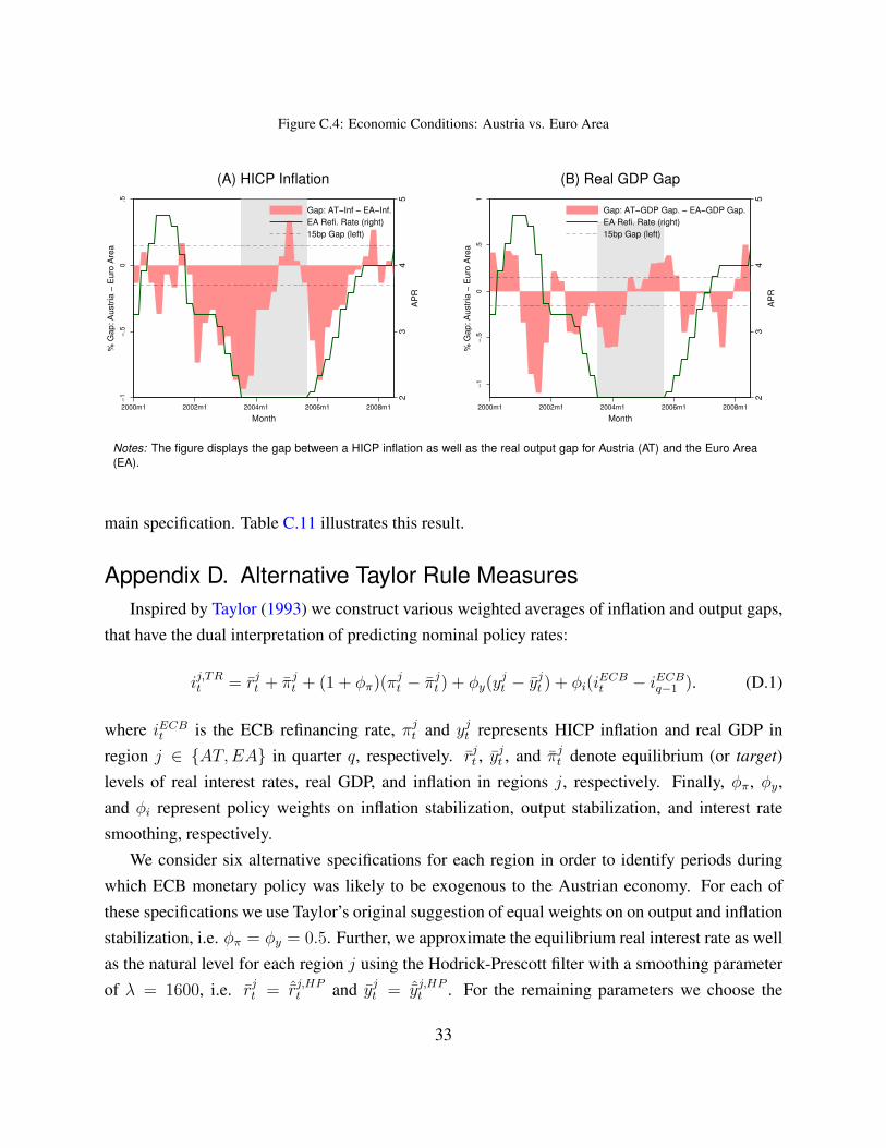
Figure C.4: Economic Conditions: Austria vs. Euro Area

(A) HICP Inflation (B) Real GDP Gap

23

45

AP

R

−1

−.5

0.5

% G

ap

: A

ustr

ia −

Eu

ro A

rea

2000m1 2002m1 2004m1 2006m1 2008m1

Month

Gap: AT−Inf − EA−Inf.

EA Refi. Rate (right)

15bp Gap (left)

23

45

AP

R

−1

−.5

0.5

1

% G

ap

: A

ustr

ia −

Eu

ro A

rea

2000m1 2002m1 2004m1 2006m1 2008m1

Month

Gap: AT−GDP Gap. − EA−GDP Gap.

EA Refi. Rate (right)

15bp Gap (left)

Notes: The figure displays the gap between a HICP inflation as well as the real output gap for Austria (AT) and the Euro Area(EA).

main specification. Table C.11 illustrates this result.

Appendix D. Alternative Taylor Rule MeasuresInspired by Taylor (1993) we construct various weighted averages of inflation and output gaps,

that have the dual interpretation of predicting nominal policy rates:

ij,TRt = rjt + πjt + (1 + φπ)(πjt − πjt ) + φy(y

jt − y

jt ) + φi(i

ECBt − iECBq−1 ). (D.1)

where iECBt is the ECB refinancing rate, πjt and yjt represents HICP inflation and real GDP inregion j ∈ {AT,EA} in quarter q, respectively. rjt , y

jt , and πjt denote equilibrium (or target)

levels of real interest rates, real GDP, and inflation in regions j, respectively. Finally, φπ, φy,and φi represent policy weights on inflation stabilization, output stabilization, and interest ratesmoothing, respectively.

We consider six alternative specifications for each region in order to identify periods duringwhich ECB monetary policy was likely to be exogenous to the Austrian economy. For each ofthese specifications we use Taylor’s original suggestion of equal weights on on output and inflationstabilization, i.e. φπ = φy = 0.5. Further, we approximate the equilibrium real interest rate as wellas the natural level for each region j using the Hodrick-Prescott filter with a smoothing parameterof λ = 1600, i.e. rjt = ˆrj,HPt and yjt = ˆyj,HPt . For the remaining parameters we choose the

33

Figure D.5: Alternative Taylor Rule Specifications

(A.1) Average Inflation (A.2) Average Inflation (Dynamic)−

20

24

6

AP

R

1999q1 2002q1 2005q1 2008q1 2011q1

Quarter

ECB Refi. Rate

Taylor Rule (AT Data)

Taylor Rule (EA Data)

−2

02

46

AP

R

1999q1 2002q1 2005q1 2008q1 2011q1

Quarter

ECB Refi. Rate

Taylor Rule (AT Data)

Taylor Rule (EA Data)

(B.1) Inflation Target of 2% (B.2) Inflation Target of 2% (Dynamic)

−2

02

46

8

AP

R

1999q1 2002q1 2005q1 2008q1 2011q1

Quarter

ECB Refi. Rate

Taylor Rule (AT Data)

Taylor Rule (EA Data)

−2

02

46

8

AP

R

1999q1 2002q1 2005q1 2008q1 2011q1

Quarter

ECB Refi. Rate

Taylor Rule (AT Data)

Taylor Rule (EA Data)

(C.1) HP Trend Inflation (C.2) HP Trend Inflation (Dynamic)

−2

02

46

8

AP

R

1999q1 2002q1 2005q1 2008q1 2011q1

Quarter

ECB Refi. Rate

Taylor Rule (AT Data)

Taylor Rule (EA Data)

−2

02

46

8

AP

R

1999q1 2002q1 2005q1 2008q1 2011q1

Quarter

ECB Refi. Rate

Taylor Rule (AT Data)

Taylor Rule (EA Data)

following six alternative specifications:

(A.1) We proxy the target inflation with average HICP inflation in Austria and the euro area, πATt =

34

2.23125 and πEAt = 2.6086905, taken over the pre EMU period 1991-1998. Further, weassume the ECB does not care about interest rate smoothing, i.e. φi = 0

(A.2) πATt = 2.23125, πEAt = 2.6086905, and φi = 0.9

(B.1) We set target inflation to 2%, i.e. πATt = πEAt = 2, and φi = 0

(B.2) πATt = πEAt = 2, and φi = 0.9

(C.1) We proxy equilibrium inflation in each region with an HP trend, i.e. πjt = ˆrj,HPt , and φi = 0

(C.2) πjt = ˆrj,HPt , and φi = 0.9

The alternative specifications highlight several important phenomena. First, Taylor’s basicspecification of φπ = φy = 0.5 does fairly well in predicting ECB refinancing rates between 1999and 2008. Second, interest smoothing motives, i.e. specifications with φi > 0, do not seem to playa significant role for the purpose of our thought experiment. Finally, and most importantly for ouranalysis, the difference between the predictions for Austria and the euro area, iAT,TRt − iEA,TRt , isvery robust across specifications.

35

Appendix E. Full Regression Tables

Table E.12: Average Effect of Lower Short Term Rate (Continuous Regressor, gapt)

Dependent Variable: Ex-Ante Expected Default Rate (EDRb,t)(1) (2) (3) (4) (5)

gap -0.0087 -0.0066 -0.0031 0.033** 0.040***(0.019) (0.018) (0.020) (0.016) (0.015)

Bank Chash: 2 0.024 -0.0029 -0.0070 -0.0061(0.035) (0.035) (0.034) (0.034)

Bank Chash: 3 0.069* 0.015 0.00094 0.0016(0.041) (0.052) (0.050) (0.050)

Bank Size: 2 0.066* -0.040 0.014 0.0069(0.040) (0.060) (0.058) (0.058)

Bank Size: 3 0.050 -0.076 0.0057 -0.012(0.041) (0.083) (0.075) (0.075)

Bank Capital: 2 0.043 0.017 0.012 0.0093(0.043) (0.037) (0.038) (0.038)

Bank Capital: 3 0.070 -0.036 -0.025 -0.032(0.044) (0.043) (0.046) (0.046)

Bank Capital: 4 0.087* -0.023 0.0092 -0.0027(0.051) (0.054) (0.060) (0.060)

Bank Capital: 5 0.039 -0.37 -0.30 -0.31(0.080) (0.23) (0.21) (0.22)

AT: Real GDP Gap -0.040*** -0.0098(0.014) (0.020)

AT: HICP Inflation 0.022 0.025(0.016) (0.019)

AT: 10-year yieald spread 0.032 0.037*(0.021) (0.021)

Diff. 10-yr. spr. (AT vs. EA) -0.37* -0.011(0.22) (0.15)

AT: Frac. Business Loans 0.014* 0.023**(0.0078) (0.0099)

AT: GKE/Total AT Loans -0.63 -0.86(0.62) (0.63)

AT: loan growth 0.0061* 0.0038(0.0036) (0.0041)

t 0.0070**(0.0029)

t2 -0.000060**(0.000029)

Constant 0.52*** 0.41***(0.021) (0.048)

Bank FEs yes yes yes

No. Banks 316 316 316 316 316Obs. 27082 27082 27082 27082 27082

Notes: The dependent variable is the ex-ante expected default rate (EDRb,t) at the banklevel. Standard errors are reported in parantheses below each coefficient and are two-wayclustered on bank and year-month following Cameron et al. (2011). Significance levels areindicated by * p < 0.1, ** p < 0.05, and *** p < 0.01.

36

Table E.13: Average Effect of Lower Short Term Rate (Discrete Regressor, GAP0.25t )

Dependent Variable: Ex-Ante Expected Default Rate (EDRb,t)(1) (2) (3) (4) (5)

GAP -0.024 -0.021 -0.020 0.016 0.038(0.026) (0.025) (0.025) (0.029) (0.026)

Bank Chash: 2 0.019 -0.0088 -0.0022 -0.0017(0.039) (0.043) (0.043) (0.043)

Bank Chash: 3 0.066 0.0032 0.0075 0.0083(0.048) (0.059) (0.058) (0.058)

Bank Size: 2 0.088** -0.0060 0.020 0.019(0.042) (0.065) (0.062) (0.062)

Bank Size: 3 0.071 -0.029 -0.0076 -0.011(0.045) (0.093) (0.079) (0.080)

Bank Capital: 2 0.050 0.034 0.018 0.018(0.040) (0.038) (0.038) (0.038)

Bank Capital: 3 0.096** -0.00063 -0.022 -0.024(0.042) (0.042) (0.046) (0.047)

Bank Capital: 4 0.13** 0.044 0.012 0.010(0.050) (0.053) (0.058) (0.058)

Bank Capital: 5 0.073 -0.31 -0.33 -0.33(0.079) (0.25) (0.24) (0.24)

AT: Real GDP Gap -0.097*** -0.056(0.022) (0.056)

AT: HICP Inflation 0.070*** 0.049**(0.026) (0.019)

AT: 10-year yieald spread 0.0080 0.018(0.031) (0.039)

Diff. 10-yr. spr. (AT vs. EA) -0.27 -0.13(0.29) (0.28)

AT: Frac. Business Loans 0.0036 0.014*(0.0094) (0.0071)

AT: GKE/Total AT Loans -2.95*** -2.76**(0.79) (1.18)

AT: loan growth 0.0031 0.00072(0.0044) (0.0037)

t 0.0052(0.0046)

t2 -0.000045(0.000048)

Constant 0.56*** 0.42***(0.024) (0.052)

Bank FEs yes yes yes

No. Banks 316 316 316 316 316Obs. 15827 15827 15827 15827 15827

Notes: The dependent variable is the ex-ante expected default rate (EDRb,t) at the banklevel. Standard errors are reported in parantheses below each coefficients and are two-wayclustered on bank and year-month following Cameron et al. (2011). Significance levels areindicated by * p < 0.1, ** p < 0.05, and *** p < 0.01.

37

Table E.14: Split Sample: Pre/Treatment/Post

A. Continuous Regressor (gapt) B. Discrete Regressor (GAP0.25t )

Pre Treat Post Pre Treat Post(A.1) (A.2) (A.3) (B.1) (B.2) (B.3)

gap -0.024** 0.064** 0.050(0.0093) (0.024) (0.040)

GAP -0.24** 0.19** -0.46***(0.087) (0.083) (0.067)

Bank Chash: 2 -0.026 -0.043 -0.053* 0.084 -0.046 -0.066(0.082) (0.083) (0.027) (0.089) (0.073) (0.040)

Bank Chash: 3 0.054 -0.13 -0.024 0.063 -0.11 -0.037(0.11) (0.11) (0.051) (0.13) (0.098) (0.068)

Bank Size: 2 -0.073 -0.10 -0.0024 -0.12 -0.068 -0.033(0.076) (0.074) (0.077) (0.093) (0.075) (0.086)

Bank Size: 3 -0.15 -0.23** -0.057 -0.17 -0.22* -0.076(0.10) (0.10) (0.082) (0.12) (0.12) (0.087)

Bank Capital: 2 -0.022 0.060 0.071* 0.018 0.040 0.074(0.046) (0.064) (0.039) (0.050) (0.061) (0.046)

Bank Capital: 3 -0.024 -0.032 0.014 0.011 -0.053 -0.00070(0.062) (0.080) (0.058) (0.078) (0.082) (0.068)

Bank Capital: 4 -0.10 0.069 -0.040 0.016 0.013 -0.033(0.12) (0.13) (0.096) (0.13) (0.15) (0.12)

Bank Capital: 5 -0.25* -0.94 -0.18* -0.89 -0.26*(0.14) (0.74) (0.10) (0.67) (0.13)

AT: Real GDP Gap 0.034 -0.024 -0.16*** 0.019* -0.12 -0.29(0.022) (0.061) (0.015) (0.010) (0.14) (0.24)

AT: HICP Inflation 0.058*** -0.029 -0.0094 0.0052 -0.16 0.19*(0.017) (0.044) (0.041) (0.028) (0.16) (0.10)

AT: 10-year yieald spread 0.071** 0.013 -0.15** 0.0082* -0.056 -0.46(0.027) (0.018) (0.059) (0.0043) (0.084) (0.33)

Diff. 10-yr. spr. (AT vs. EA) 0.81* 0.23 3.67*** 0.21 -0.54 3.17(0.45) (0.62) (0.048) (0.31) (0.54) (3.85)

AT: Frac. Business Loans -0.0081 -0.020 0.012 0.0089 -0.015 -0.035***(0.0071) (0.029) (0.020) (0.023) (0.017) (0.0098)

AT: GKE/Total AT Loans 0.64*** -0.84*** -2.52*** 0.26*** -0.90*** -1.73(0.16) (0.049) (0.018) (0.043) (0.092) (1.30)

AT: loan growth -0.012** 0.0010 -0.018 0.0034 0.00011 0.0053(0.0046) (0.0026) (0.013) (0.0024) (0.0011) (0.010)

t 0.0083 -0.028 -0.023 -0.0042*** 0.0063 -0.047(0.0051) (0.039) (0.045) (0.0014) (0.012) (0.030)

t2 -0.000040 0.00028 0.00010 0.000039 -0.000011 0.00024(0.00014) (0.00039) (0.00027) (0.00011) (0.00012) (0.00022)

Bank FEs yes yes yes yes yes yes

No. Banks 282 288 310 280 288 310Obs. 9903 7186 9991 4950 5616 5260

Notes: The dependent variable is the ex-ante expected default rate (EDRb,t) at the bank level. Standard errorsare reported in parantheses below each coefficient and are two-way clustered on bank and year-month followingCameron et al. (2011). Significance levels are indicated by * p < 0.1, ** p < 0.05, and *** p < 0.01.

38

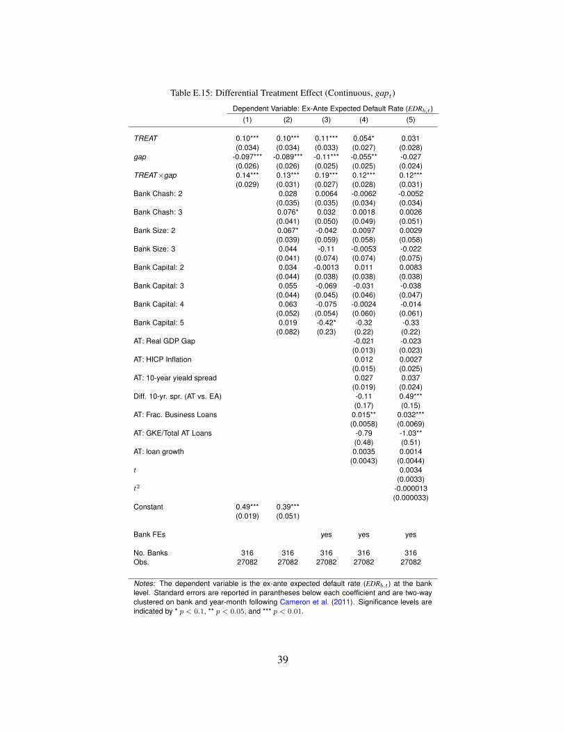
Table E.15: Differential Treatment Effect (Continuous, gapt)

Dependent Variable: Ex-Ante Expected Default Rate (EDRb,t)(1) (2) (3) (4) (5)

TREAT 0.10*** 0.10*** 0.11*** 0.054* 0.031(0.034) (0.034) (0.033) (0.027) (0.028)

gap -0.097*** -0.089*** -0.11*** -0.055** -0.027(0.026) (0.026) (0.025) (0.025) (0.024)

TREAT×gap 0.14*** 0.13*** 0.19*** 0.12*** 0.12***(0.029) (0.031) (0.027) (0.028) (0.031)

Bank Chash: 2 0.028 0.0064 -0.0062 -0.0052(0.035) (0.035) (0.034) (0.034)

Bank Chash: 3 0.076* 0.032 0.0018 0.0026(0.041) (0.050) (0.049) (0.051)

Bank Size: 2 0.067* -0.042 0.0097 0.0029(0.039) (0.059) (0.058) (0.058)

Bank Size: 3 0.044 -0.11 -0.0053 -0.022(0.041) (0.074) (0.074) (0.075)

Bank Capital: 2 0.034 -0.0013 0.011 0.0083(0.044) (0.038) (0.038) (0.038)

Bank Capital: 3 0.055 -0.069 -0.031 -0.038(0.044) (0.045) (0.046) (0.047)

Bank Capital: 4 0.063 -0.075 -0.0024 -0.014(0.052) (0.054) (0.060) (0.061)

Bank Capital: 5 0.019 -0.42* -0.32 -0.33(0.082) (0.23) (0.22) (0.22)

AT: Real GDP Gap -0.021 -0.023(0.013) (0.023)

AT: HICP Inflation 0.012 0.0027(0.015) (0.025)

AT: 10-year yieald spread 0.027 0.037(0.019) (0.024)

Diff. 10-yr. spr. (AT vs. EA) -0.11 0.49***(0.17) (0.15)

AT: Frac. Business Loans 0.015** 0.032***(0.0058) (0.0069)

AT: GKE/Total AT Loans -0.79 -1.03**(0.48) (0.51)

AT: loan growth 0.0035 0.0014(0.0043) (0.0044)

t 0.0034(0.0033)

t2 -0.000013(0.000033)

Constant 0.49*** 0.39***(0.019) (0.051)

Bank FEs yes yes yes

No. Banks 316 316 316 316 316Obs. 27082 27082 27082 27082 27082

Notes: The dependent variable is the ex-ante expected default rate (EDRb,t) at the banklevel. Standard errors are reported in parantheses below each coefficient and are two-wayclustered on bank and year-month following Cameron et al. (2011). Significance levels areindicated by * p < 0.1, ** p < 0.05, and *** p < 0.01.

39

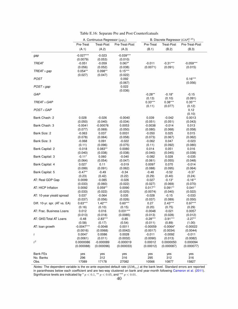
Table E.16: Separate Pre and Post Counterfcatuals

A. Continuous Regressor (gapt) B. Discrete Regressor (GAP0.25t )

Pre-Treat Treat-Post Pre-Treat-Post Pre-Treat Treat-Post Pre-Treat-Post(A.1) (A.2) (A.3) (B.1) (B.2) (B.3)

gap -0.027*** -0.023 -0.039***(0.0079) (0.053) (0.010)

TREAT -0.051 -0.059 0.067* -0.011 -0.31*** -0.059***(0.056) (0.052) (0.038) (0.0071) (0.091) (0.015)

TREAT×gap 0.054** 0.098** 0.15***(0.027) (0.047) (0.022)

POST 0.092 0.16***(0.067) (0.056)

POST×gap 0.022(0.036)

GAP -0.28** -0.18* -0.15(0.13) (0.10) (0.091)

TREAT×GAP 0.33*** 0.38*** 0.35***(0.11) (0.077) (0.12)

POST×GAP 0.12(0.10)

Bank Chash: 2 0.028 -0.026 -0.0040 0.039 -0.042 0.0013(0.050) (0.040) (0.034) (0.051) (0.051) (0.043)

Bank Chash: 3 -0.0041 -0.00076 0.0053 -0.0038 -0.014 0.013(0.077) (0.069) (0.050) (0.080) (0.068) (0.058)

Bank Size: 2 -0.063 0.037 0.0031 -0.050 0.025 0.015(0.078) (0.064) (0.058) (0.073) (0.067) (0.062)

Bank Size: 3 -0.068 0.091 -0.022 -0.062 0.047 -0.023(0.11) (0.096) (0.075) (0.11) (0.092) (0.080)

Bank Capital: 2 -0.018 0.083** 0.0080 0.014 0.051 0.016(0.040) (0.038) (0.038) (0.040) (0.045) (0.038)

Bank Capital: 3 -0.11* 0.060 -0.040 -0.082 0.028 -0.035(0.064) (0.054) (0.047) (0.061) (0.055) (0.048)

Bank Capital: 4 0.027 0.11 -0.019 0.0097 0.070 -0.014(0.099) (0.091) (0.062) (0.088) (0.095) (0.064)

Bank Capital: 5 -0.47** -0.49 -0.34 -0.48 -0.52 -0.37(0.23) (0.42) (0.22) (0.29) (0.40) (0.24)

AT: Real GDP Gap 0.0099 -0.085 -0.026 -0.027 -0.13* -0.16**(0.033) (0.060) (0.022) (0.027) (0.069) (0.070)

AT: HICP Inflation 0.0092 0.059** 0.0090 0.017** 0.091** 0.041*(0.033) (0.022) (0.025) (0.0074) (0.040) (0.022)

AT: 10-year yieald spread 0.037 -0.064 0.035 -0.028 -0.15 -0.033(0.037) (0.056) (0.026) (0.037) (0.089) (0.050)

Diff. 10-yr. spr. (AT vs. EA) 0.63*** 1.42*** 0.60*** 0.27 2.43*** 0.97***(0.16) (0.10) (0.15) (0.20) (0.75) (0.29)

AT: Frac. Business Loans 0.012 0.016 0.031*** -0.0048 -0.021 0.0057(0.013) (0.018) (0.0085) (0.013) (0.028) (0.012)

AT: GKE/Total AT Loans -0.48 -2.83*** -0.85 -0.28*** -3.91*** -2.27**(0.58) (0.17) (0.54) (0.011) (0.89) (1.00)

AT: loan growth -0.0047*** -0.0048 0.0011 -0.00059 -0.0064* -0.00022(0.0016) (0.0068) (0.0042) (0.0017) (0.0034) (0.0044)

t 0.0047 0.0086 0.0028 -0.011 -0.0092 -0.011(0.0061) (0.011) (0.0032) (0.0090) (0.013) (0.0082)

t2 0.0000086 -0.000089 -0.000019 0.00012 0.0000050 0.000094(0.000088) (0.000096) (0.000033) (0.00012) (0.000087) (0.000077)

Bank FEs yes yes yes yes yes yesNo. Banks 296 312 316 295 312 316Obs. 17089 17178 27082 10566 10877 15827

Notes: The dependent variable is the ex-ante expected default rate (EDRb,t) at the bank level. Standard errors are reportedin parantheses below each coefficient and are two-way clustered on bank and year-month following Cameron et al. (2011).Significance levels are indicated by * p < 0.1, ** p < 0.05, and *** p < 0.01.

40

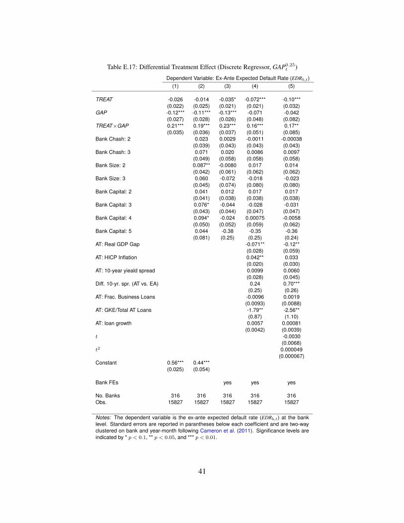
Table E.17: Differential Treatment Effect (Discrete Regressor, GAP0.25t )

Dependent Variable: Ex-Ante Expected Default Rate (EDRb,t)(1) (2) (3) (4) (5)

TREAT -0.026 -0.014 -0.035* -0.072*** -0.10***(0.022) (0.025) (0.021) (0.021) (0.032)

GAP -0.12*** -0.11*** -0.13*** -0.071 -0.042(0.027) (0.028) (0.026) (0.048) (0.082)

TREAT×GAP 0.21*** 0.19*** 0.23*** 0.16*** 0.17**(0.035) (0.036) (0.037) (0.051) (0.085)

Bank Chash: 2 0.023 0.0029 -0.0011 -0.00038(0.039) (0.043) (0.043) (0.043)

Bank Chash: 3 0.071 0.020 0.0086 0.0097(0.049) (0.058) (0.058) (0.058)

Bank Size: 2 0.087** -0.0080 0.017 0.014(0.042) (0.061) (0.062) (0.062)

Bank Size: 3 0.060 -0.072 -0.018 -0.023(0.045) (0.074) (0.080) (0.080)

Bank Capital: 2 0.041 0.012 0.017 0.017(0.041) (0.038) (0.038) (0.038)

Bank Capital: 3 0.076* -0.044 -0.028 -0.031(0.043) (0.044) (0.047) (0.047)

Bank Capital: 4 0.094* -0.024 0.00075 -0.0058(0.050) (0.052) (0.059) (0.062)

Bank Capital: 5 0.044 -0.38 -0.35 -0.36(0.081) (0.25) (0.25) (0.24)

AT: Real GDP Gap -0.071** -0.12**(0.028) (0.059)

AT: HICP Inflation 0.042** 0.033(0.020) (0.030)

AT: 10-year yieald spread 0.0099 0.0060(0.028) (0.045)

Diff. 10-yr. spr. (AT vs. EA) 0.24 0.70***(0.25) (0.26)

AT: Frac. Business Loans -0.0096 0.0019(0.0093) (0.0088)

AT: GKE/Total AT Loans -1.79** -2.56**(0.87) (1.10)

AT: loan growth 0.0057 0.00081(0.0042) (0.0039)

t -0.0030(0.0068)

t2 0.000049(0.000067)

Constant 0.56*** 0.44***(0.025) (0.054)

Bank FEs yes yes yes

No. Banks 316 316 316 316 316Obs. 15827 15827 15827 15827 15827

Notes: The dependent variable is the ex-ante expected default rate (EDRb,t) at the banklevel. Standard errors are reported in parantheses below each coefficient and are two-wayclustered on bank and year-month following Cameron et al. (2011). Significance levels areindicated by * p < 0.1, ** p < 0.05, and *** p < 0.01.

41

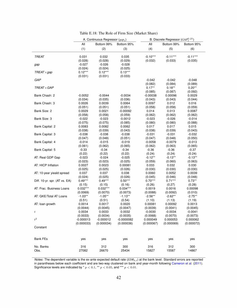
Table E.18: The Role of Firm Size (Market Share)

A. Continuous Regressor (gapt) B. Discrete Regressor (GAP0.25t )

All Bottom 99% Bottom 95% All Bottom 99% Bottom 95%(1) (2) (3) (4) (5) (6)

TREAT 0.031 0.032 0.035 -0.10*** -0.11*** -0.11***(0.028) (0.028) (0.029) (0.032) (0.033) (0.035)

gap -0.027 -0.026 -0.028(0.024) (0.024) (0.025)

TREAT×gap 0.12*** 0.12*** 0.13***(0.031) (0.031) (0.033)

GAP -0.042 -0.042 -0.048(0.082) (0.084) (0.089)

TREAT×GAP 0.17** 0.18** 0.20**(0.085) (0.087) (0.092)

Bank Chash: 2 -0.0052 -0.0044 -0.0034 -0.00038 0.00096 0.0029(0.034) (0.035) (0.036) (0.043) (0.043) (0.044)

Bank Chash: 3 0.0026 0.0039 0.0064 0.0097 0.012 0.016(0.051) (0.051) (0.051) (0.058) (0.058) (0.059)

Bank Size: 2 0.0029 0.0021 -0.00092 0.014 0.013 0.0087(0.058) (0.058) (0.059) (0.062) (0.062) (0.062)

Bank Size: 3 -0.022 -0.023 -0.0012 -0.023 -0.026 -0.014(0.075) (0.075) (0.085) (0.080) (0.080) (0.088)

Bank Capital: 2 0.0083 0.0082 0.0062 0.017 0.017 0.015(0.038) (0.039) (0.043) (0.038) (0.039) (0.043)

Bank Capital: 3 -0.038 -0.038 -0.038 -0.031 -0.031 -0.032(0.047) (0.048) (0.051) (0.047) (0.048) (0.050)

Bank Capital: 4 -0.014 -0.015 -0.019 -0.0058 -0.0079 -0.013(0.061) (0.062) (0.065) (0.062) (0.063) (0.065)

Bank Capital: 5 -0.33 -0.34 -0.34 -0.36 -0.36 -0.37(0.22) (0.22) (0.22) (0.24) (0.24) (0.24)

AT: Real GDP Gap -0.023 -0.024 -0.025 -0.12** -0.13** -0.13**(0.023) (0.023) (0.025) (0.059) (0.060) (0.063)

AT: HICP Inflation 0.0027 0.0023 0.00081 0.033 0.032 0.030(0.025) (0.025) (0.026) (0.030) (0.030) (0.030)

AT: 10-year yieald spread 0.037 0.037 0.038 0.0060 0.0052 0.0039(0.024) (0.025) (0.026) (0.045) (0.046) (0.048)

Diff. 10-yr. spr. (AT vs. EA) 0.49*** 0.49*** 0.50*** 0.70*** 0.71*** 0.73**(0.15) (0.15) (0.16) (0.26) (0.27) (0.28)

AT: Frac. Business Loans 0.032*** 0.032*** 0.034*** 0.0019 0.0016 0.00098(0.0069) (0.0070) (0.0073) (0.0088) (0.0092) (0.010)

AT: GKE/Total AT Loans -1.03** -1.05** -1.13** -2.56** -2.62** -2.75**(0.51) (0.51) (0.54) (1.10) (1.13) (1.19)

AT: loan growth 0.0014 0.0017 0.0020 0.00081 0.00092 0.0013(0.0044) (0.0045) (0.0047) (0.0039) (0.0041) (0.0045)

t 0.0034 0.0033 0.0032 -0.0030 -0.0034 -0.0041(0.0033) (0.0034) (0.0035) (0.0068) (0.0070) (0.0073)

t2 -0.000013 -0.000012 -0.0000082 0.000049 0.000053 0.000062(0.000033) (0.000034) (0.000036) (0.000067) (0.000069) (0.000072)

Constant

Bank FEs yes yes yes yes yes yes

No. Banks 316 312 300 316 312 300Obs. 27082 26670 25434 15827 15587 14867

Notes: The dependent variable is the ex-ante expected default rate (EDRb,t) at the bank level. Standard errors are reportedin parantheses below each coefficient and are two-way clustered on bank and year-month following Cameron et al. (2011).Significance levels are indicated by * p < 0.1, ** p < 0.05, and *** p < 0.01.

42

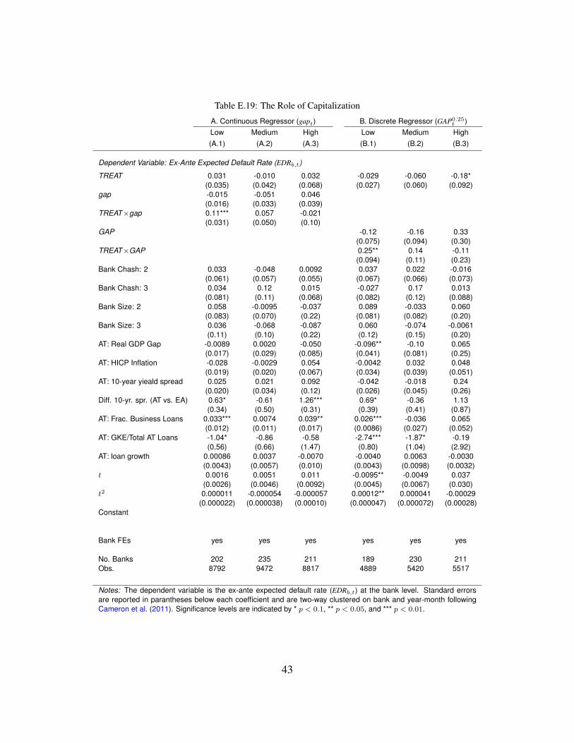
Table E.19: The Role of Capitalization

A. Continuous Regressor (gapt) B. Discrete Regressor (GAP0.25t )

Low Medium High Low Medium High(A.1) (A.2) (A.3) (B.1) (B.2) (B.3)

Dependent Variable: Ex-Ante Expected Default Rate (EDRb,t)

TREAT 0.031 -0.010 0.032 -0.029 -0.060 -0.18*(0.035) (0.042) (0.068) (0.027) (0.060) (0.092)

gap -0.015 -0.051 0.046(0.016) (0.033) (0.039)

TREAT×gap 0.11*** 0.057 -0.021(0.031) (0.050) (0.10)

GAP -0.12 -0.16 0.33(0.075) (0.094) (0.30)

TREAT×GAP 0.25** 0.14 -0.11(0.094) (0.11) (0.23)

Bank Chash: 2 0.033 -0.048 0.0092 0.037 0.022 -0.016(0.061) (0.057) (0.055) (0.067) (0.066) (0.073)

Bank Chash: 3 0.034 0.12 0.015 -0.027 0.17 0.013(0.081) (0.11) (0.068) (0.082) (0.12) (0.088)

Bank Size: 2 0.058 -0.0095 -0.037 0.089 -0.033 0.060(0.083) (0.070) (0.22) (0.081) (0.082) (0.20)

Bank Size: 3 0.036 -0.068 -0.087 0.060 -0.074 -0.0061(0.11) (0.10) (0.22) (0.12) (0.15) (0.20)

AT: Real GDP Gap -0.0089 0.0020 -0.050 -0.096** -0.10 0.065(0.017) (0.029) (0.085) (0.041) (0.081) (0.25)

AT: HICP Inflation -0.028 -0.0029 0.054 -0.0042 0.032 0.048(0.019) (0.020) (0.067) (0.034) (0.039) (0.051)

AT: 10-year yieald spread 0.025 0.021 0.092 -0.042 -0.018 0.24(0.020) (0.034) (0.12) (0.026) (0.045) (0.26)

Diff. 10-yr. spr. (AT vs. EA) 0.63* -0.61 1.26*** 0.69* -0.36 1.13(0.34) (0.50) (0.31) (0.39) (0.41) (0.87)

AT: Frac. Business Loans 0.033*** 0.0074 0.039** 0.026*** -0.036 0.065(0.012) (0.011) (0.017) (0.0086) (0.027) (0.052)

AT: GKE/Total AT Loans -1.04* -0.86 -0.58 -2.74*** -1.87* -0.19(0.56) (0.66) (1.47) (0.80) (1.04) (2.92)

AT: loan growth 0.00086 0.0037 -0.0070 -0.0040 0.0063 -0.0030(0.0043) (0.0057) (0.010) (0.0043) (0.0098) (0.0032)

t 0.0016 0.0051 0.011 -0.0095** -0.0049 0.037(0.0026) (0.0046) (0.0092) (0.0045) (0.0067) (0.030)

t2 0.000011 -0.000054 -0.000057 0.00012** 0.000041 -0.00029(0.000022) (0.000038) (0.00010) (0.000047) (0.000072) (0.00028)

Constant

Bank FEs yes yes yes yes yes yes

No. Banks 202 235 211 189 230 211Obs. 8792 9472 8817 4889 5420 5517

Notes: The dependent variable is the ex-ante expected default rate (EDRb,t) at the bank level. Standard errorsare reported in parantheses below each coefficient and are two-way clustered on bank and year-month followingCameron et al. (2011). Significance levels are indicated by * p < 0.1, ** p < 0.05, and *** p < 0.01.

43

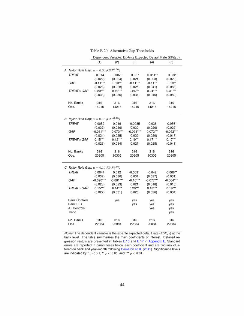
Table E.20: Alternative Gap Thresholds

Dependent Variable: Ex-Ante Expected Default Rate (EDRb,t)(1) (2) (3) (4) (5)

A. Taylor Rule Gap: µ = 0.30 (GAP0.30t )

TREAT -0.014 -0.0079 -0.027 -0.051** -0.032(0.022) (0.024) (0.021) (0.023) (0.029)

GAP -0.11*** -0.10*** -0.11*** -0.11** -0.19**(0.028) (0.028) (0.025) (0.041) (0.088)

TREAT×GAP 0.20*** 0.19*** 0.24*** 0.24*** 0.31***(0.033) (0.036) (0.034) (0.046) (0.089)

No. Banks 316 316 316 316 316Obs. 14215 14215 14215 14215 14215

B. Taylor Rule Gap: µ = 0.15 (GAP0.15t )

TREAT 0.0052 0.016 -0.0085 -0.036 -0.056*(0.032) (0.036) (0.030) (0.026) (0.029)

GAP -0.081*** -0.070*** -0.098*** -0.072*** -0.052***(0.024) (0.025) (0.022) (0.020) (0.017)

TREAT×GAP 0.15*** 0.12*** 0.19*** 0.17*** 0.17***(0.028) (0.034) (0.027) (0.025) (0.041)

No. Banks 316 316 316 316 316Obs. 20305 20305 20305 20305 20305

C. Taylor Rule Gap: µ = 0.10 (GAP0.10t )

TREAT 0.0044 0.012 -0.0091 -0.042 -0.066**(0.032) (0.036) (0.031) (0.027) (0.031)

GAP -0.090*** -0.081*** -0.10*** -0.077*** -0.064***(0.023) (0.023) (0.021) (0.018) (0.015)

TREAT×GAP 0.15*** 0.14*** 0.20*** 0.18*** 0.19***(0.027) (0.031) (0.026) (0.026) (0.034)

Bank Controls yes yes yes yesBank FEs yes yes yesAT Controls yes yesTrend yes

No. Banks 316 316 316 316 316Obs. 22884 22884 22884 22884 22884

Notes: The dependent variable is the ex-ante expected default rate (EDRb,t) at thebank level. The table summarizes the main coefficients of interest. Detailed re-gression restuls are presented in Tables E.15 and E.17 in Appendix E. Standarderrors are reported in parantheses below each coefficient and are two-way clus-tered on bank and year-month following Cameron et al. (2011). Significance levelsare indicated by * p < 0.1, ** p < 0.05, and *** p < 0.01.

44

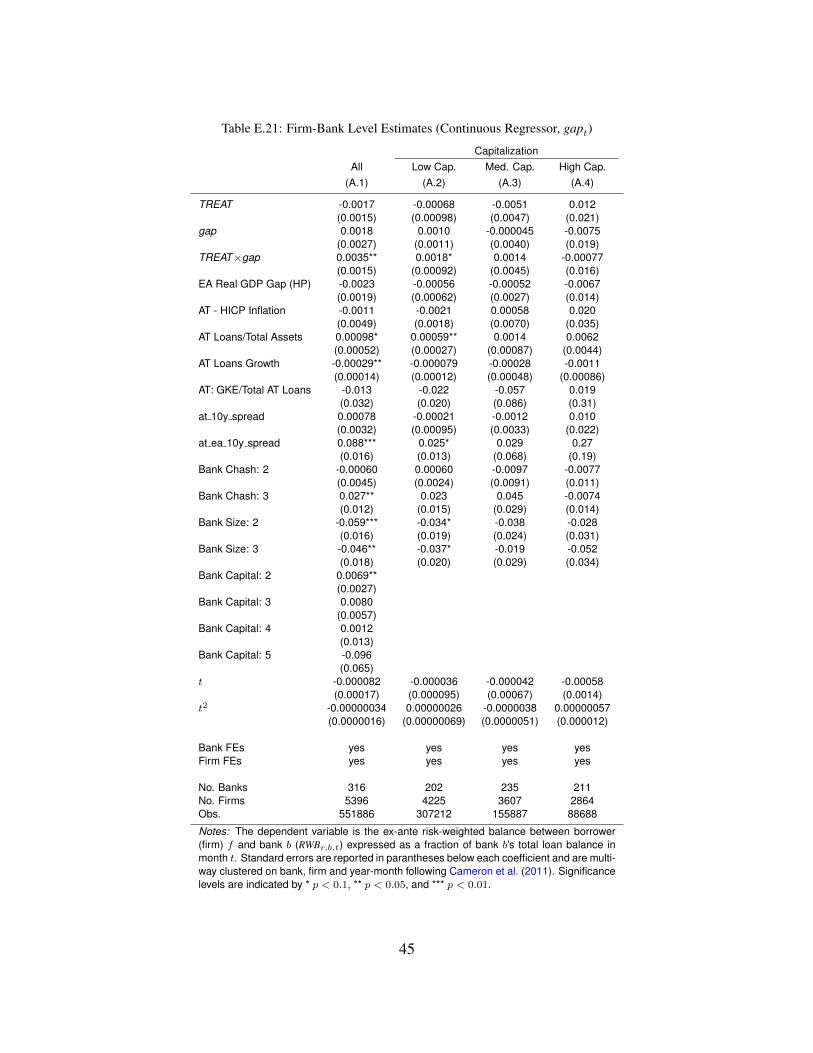
Table E.21: Firm-Bank Level Estimates (Continuous Regressor, gapt)

CapitalizationAll Low Cap. Med. Cap. High Cap.

(A.1) (A.2) (A.3) (A.4)

TREAT -0.0017 -0.00068 -0.0051 0.012(0.0015) (0.00098) (0.0047) (0.021)

gap 0.0018 0.0010 -0.000045 -0.0075(0.0027) (0.0011) (0.0040) (0.019)

TREAT×gap 0.0035** 0.0018* 0.0014 -0.00077(0.0015) (0.00092) (0.0045) (0.016)

EA Real GDP Gap (HP) -0.0023 -0.00056 -0.00052 -0.0067(0.0019) (0.00062) (0.0027) (0.014)

AT - HICP Inflation -0.0011 -0.0021 0.00058 0.020(0.0049) (0.0018) (0.0070) (0.035)

AT Loans/Total Assets 0.00098* 0.00059** 0.0014 0.0062(0.00052) (0.00027) (0.00087) (0.0044)

AT Loans Growth -0.00029** -0.000079 -0.00028 -0.0011(0.00014) (0.00012) (0.00048) (0.00086)

AT: GKE/Total AT Loans -0.013 -0.022 -0.057 0.019(0.032) (0.020) (0.086) (0.31)

at 10y spread 0.00078 -0.00021 -0.0012 0.010(0.0032) (0.00095) (0.0033) (0.022)

at ea 10y spread 0.088*** 0.025* 0.029 0.27(0.016) (0.013) (0.068) (0.19)

Bank Chash: 2 -0.00060 0.00060 -0.0097 -0.0077(0.0045) (0.0024) (0.0091) (0.011)

Bank Chash: 3 0.027** 0.023 0.045 -0.0074(0.012) (0.015) (0.029) (0.014)

Bank Size: 2 -0.059*** -0.034* -0.038 -0.028(0.016) (0.019) (0.024) (0.031)

Bank Size: 3 -0.046** -0.037* -0.019 -0.052(0.018) (0.020) (0.029) (0.034)

Bank Capital: 2 0.0069**(0.0027)

Bank Capital: 3 0.0080(0.0057)

Bank Capital: 4 0.0012(0.013)

Bank Capital: 5 -0.096(0.065)

t -0.000082 -0.000036 -0.000042 -0.00058(0.00017) (0.000095) (0.00067) (0.0014)

t2 -0.00000034 0.00000026 -0.0000038 0.00000057(0.0000016) (0.00000069) (0.0000051) (0.000012)

Bank FEs yes yes yes yesFirm FEs yes yes yes yes

No. Banks 316 202 235 211No. Firms 5396 4225 3607 2864Obs. 551886 307212 155887 88688

Notes: The dependent variable is the ex-ante risk-weighted balance between borrower(firm) f and bank b (RWBr,b,t) expressed as a fraction of bank b’s total loan balance inmonth t. Standard errors are reported in parantheses below each coefficient and are multi-way clustered on bank, firm and year-month following Cameron et al. (2011). Significancelevels are indicated by * p < 0.1, ** p < 0.05, and *** p < 0.01.

45

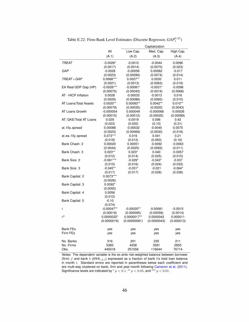
Table E.22: Firm-Bank Level Estimates (Discrete Regressor, GAP0.25t )

CapitalizationAll Low Cap. Med. Cap. High Cap.

(A.1) (A.2) (A.3) (A.4)

TREAT -0.0028* -0.0010 -0.0044 0.0096(0.0017) (0.0014) (0.0070) (0.023)

GAP -0.0026 -0.00056 0.00082 -0.017(0.0023) (0.00090) (0.0074) (0.014)

TREAT×GAP 0.0068*** 0.0027** 0.0030 0.011(0.0021) (0.0013) (0.0063) (0.019)

EA Real GDP Gap (HP) -0.0026*** -0.00081* -0.0031* -0.0096(0.00070) (0.00042) (0.0019) (0.0068)

AT - HICP Inflation 0.0028 -0.00033 -0.0013 0.016(0.0029) (0.00086) (0.0060) (0.010)

AT Loans/Total Assets 0.0020** 0.00083** 0.0042** 0.010**(0.00079) (0.00035) (0.0020) (0.0043)

AT Loans Growth -0.000054 0.000049 -0.000068 -0.00026(0.00015) (0.00012) (0.00035) (0.00089)

AT: GKE/Total AT Loans 0.029 -0.0019 0.096 0.42(0.023) (0.020) (0.10) (0.31)

at 10y spread 0.00088 -0.00032 -0.0045 0.0075(0.0023) (0.00069) (0.0030) (0.018)

at ea 10y spread 0.073*** 0.016 0.041 0.21(0.018) (0.012) (0.063) (0.16)

Bank Chash: 2 0.00020 0.00051 -0.0092 -0.0063(0.0044) (0.0025) (0.0083) (0.011)

Bank Chash: 3 0.023** 0.023* 0.040 -0.0057(0.012) (0.014) (0.025) (0.015)

Bank Size: 2 -0.061*** -0.029* -0.043* -0.037(0.015) (0.016) (0.024) (0.033)

Bank Size: 3 -0.045** -0.031* -0.021 -0.064*(0.017) (0.017) (0.028) (0.036)

Bank Capital: 2 0.0073***(0.0026)

Bank Capital: 3 0.0092*(0.0055)

Bank Capital: 4 0.0056(0.012)

Bank Capital: 5 -0.10(0.074)

t -0.00047** -0.00020** -0.00081 -0.0015(0.00019) (0.000095) (0.00058) (0.0014)

t2 0.0000032* 0.0000017** 0.0000043 0.000011(0.0000019) (0.00000081) (0.0000043) (0.000013)

Bank FEs yes yes yes yesFirm FEs yes yes yes yes

No. Banks 316 201 235 211No. Firms 5383 4208 3591 2855Obs. 445018 251556 116644 76714

Notes: The dependent variable is the ex-ante risk-weighted balance between borrower(firm) f and bank b (RWBr,b,t) expressed as a fraction of bank b’s total loan balancein month t. Standard errors are reported in parantheses below each coefficient andare multi-way clustered on bank, firm and year-month following Cameron et al. (2011).Significance levels are indicated by * p < 0.1, ** p < 0.05, and *** p < 0.01.

46