DocumentsÅdne Cappelen, Robin Choudhuryand Torfinn Harding

A small macroeconomic modelfor Malawi

Statistics NorwayResearch Department

2006/3 Februar 2006 Documents

1

Table of content 1. Introduction ...................................................................................................................................... 3

2. Main features of the model .............................................................................................................. 3

3. Detailed specification of sub-models ............................................................................................... 5 3.1. Introduction ................................................................................................................................ 5 3.2. Government sector...................................................................................................................... 5 3.3. Household sector ........................................................................................................................ 8 3.4. The external sector.................................................................................................................... 10 3.5. The business sector ................................................................................................................... 11 3.6. National accounts identities and adding up .............................................................................. 14 3.7. Financial programming............................................................................................................. 16

4. The baseline scenario ..................................................................................................................... 17

5. Model performance ........................................................................................................................ 19

6. Multiplier analyses ......................................................................................................................... 21 6.1. Increase in government spending ............................................................................................. 21 6.2. Increase in import price ............................................................................................................ 24

References ............................................................................................................................................ 26

Appendix 1. List of variables........................................................................................................ 27

Appendix 2. Some data issues....................................................................................................... 32 Appendix 2.1. Capital stocks ........................................................................................................ 32 Appendix 2.2. Employment .......................................................................................................... 32

Appendix 3. The model ................................................................................................................. 33

Appendix 4. Estimation results .................................................................................................... 36 Appendix 4.1. Introduction ........................................................................................................... 36 Appendix 4.2. Private consumption .............................................................................................. 37 Appendix 4.3. Price of export ....................................................................................................... 38 Appendix 4.4. Volume of exports ................................................................................................. 40 Appendix 4.5. Private sector employment .................................................................................... 41 Appendix 4.6. Factor price............................................................................................................ 43 Appendix 4.7. Consumer price ..................................................................................................... 44 Appendix 4.8. Price of investments .............................................................................................. 46

2

List of figures

Figure 1 Schematic outline of the model................................................................................... 4 Figure 2 Historical and simulated values: GDP private sector................................................ 19 Figure 3 Historical and simulated values: Private consumption.............................................. 19 Figure 4 Historical and simulated values: Wage earners private sector .................................. 20 Figure 5 Historical and simulated values: GDP deflator factor costs private sector ............... 20 Figure 6 Historical and simulated values: Deflator private consumption ............................... 20 Figure 7 Historical and simulated values: Deflator private investments ................................. 20 Figure 8 GDP, consumption, imports. ..................................................................................... 21 Figure 9 Employment and labour costs. .................................................................................. 21 Figure 10 Government revenues and expenditures. ................................................................ 22 Figure 11 Current accounts and government savings.............................................................. 22 Figure 12 Price deflators.......................................................................................................... 22 Figure 13 Simplified flow chart of the model ......................................................................... 23 Figure 14 GDP, consumption, imports. ................................................................................... 24 Figure 15 Employment and labour costs. ................................................................................ 24 Figure 16 Government revenues and expenditures. ................................................................ 25 Figure 17 Current account and government savings. .............................................................. 25 Figure 18 Price deflators.......................................................................................................... 25 Figure 19 Actual and fitted values: Non-smallholders consumption ...................................... 38 Figure 20 Actual and fitted values: Export price..................................................................... 39 Figure 21 Actual and fitted values: Volume of exports........................................................... 41 Figure 22 Actual and fitted values: Number of wage earners, private sector.......................... 42 Figure 23 Actual and fitted values: Factor price deflator, GDP private sector........................ 44 Figure 24 Actual and fitted values: Deflator non-smallholders consumption ......................... 45 Figure 25 Actual and fitted values: Deflator private investment............................................. 46

List of tables

Table 1 Baseline scenario: Main macroeconomic figures ....................................................... 17 Table 2 Baseline scenario: Central government operations..................................................... 18 Table 3 Baseline scenario: Prices and costs ............................................................................ 18 Table 4 Baseline scenario: Balance of payments .................................................................... 18 Table 5 Statistics from estimation in TROLL ......................................................................... 37

3

1. Introduction In meetings between representatives of the Malawian government and Statistics Norway in May 2004, we agreed upon developing a small and aggregated model of the Malawian economy as a first step in efforts to construct a disaggregated model based on new national accounts data for Malawi expected to become available sometime during 2006. A model project consists of many components of which one is knowledge of the software used for programming and solving the model. In order to gain some experience with the TROLL software, we agreed to start with a small model as a testing ground for later work. Also there may be delays in creating a database for a large-scale model so the project would benefit from proceeding along several independent tracks to avoid being potentially held up by delays in other parts of the overall project. A third reason is that many of the issues in econometrics and economic theory that one encounters in modelling are more or less the same irrespective of the level of aggregation. So there is a general learning potential for modelling, even by starting off by developing an aggregated model. Ending up with a small model of some hundred equations is rather on the big side, and perhaps not the best starting point. A much smaller model would serve the purpose as a training ground for learning the TROLL software. However, as applied economists we like to have some feeling of relevance when modelling. Thus the model easily becomes larger than originally contemplated even though issues relating fiscal policy and its impact on monetary conditions as well as interest rates etc. are not modelled in a satisfactory way in the present small model. On the other hand and referring back to what was said earlier, the present model of the real side of the economy (but clearly not the monetary side) is perhaps not far from how one will model various sectors later on. Hopefully many of the adding up equations and identities will be useful for a disaggregated model as well. In this document we first present the main features of model, before the various blocks of the model is more thoroughly described in Chapter 3. In Chapter 4 we present the main variables in the baseline scenario for the period 2005-2011. In Chapter 5 we study the models tracking performance by means of a historical simulation. In Chapter 6 we have used the model to simulate a fiscal shift. In Appendix 1 there is a list of all the variables in the model, and some data issues are discussed in Appendix 2. In Appendix 3 all the equations in the model is presented, and in Appendix 4 we present detailed information from estimating the econometric equations.

2. Main features of the model The structure of the small macroeconomic model can be illustrated schematically as in Figure 1. The model user will have to make assumptions with respect to a number of fiscal policy variables such as government employment and purchases, the average government wage rate, direct and indirect tax rates incl. import duties. Among the monetary variables the model user will have to fix interest rates and some financial assets such as government net lending abroad. Some variables are determined outside the Malawian economy such as demand for Malawian export produce, world market prices, foreign grants etc. Finally some other variables such as the Malawian labour force will have to be fixed. Also private investments are an exogenous variable in this model but should clearly be made endogenous at a later stage. Given these assumptions, the model will calculate a number of national account variables such as value added, price indices for value added as well as for final demand components. Financial balances in addition to the government budget balance will be determined along with some very aggregated monetary variables, like money supply and total domestic lending.

4

Figure 1 Schematic outline of the model

Fiscal policy

The macro economic model

Exogenous variables

Monetary policy

World economy

Other exogenous variables

Government expenditures and revenues

Prices, incomes, value added/GDP,

employment, exports imports, consumption

Current account, Financial balances

System of equations Endogenous variables

The model works like a simple Keynesian model if taken very literally. This means that a change in demand such as government purchases will increase incomes, employment and private consumption and thereby also GDP in the private sector. Tax revenues will increase as a consequence but not sufficient to eliminate the expenditure increase so that the government budget balance will deteriorate and increase government domestic lending. Increased demand will increase imports and increase the current account deficit. This will be financed by an increase in private net lending abroad because government lending is exogenous. If the model user does not think this is feasible he/she may have to reduce the foreign exchange reserves in order to finance the increased deficit on the current account. If world demand for Malawian exports increases for a given terms of trade, exports will increase and so will GDP. Increased incomes will again increase employment and household incomes and thereby private consumption. Tax revenues will now increase while expenditures remain unchanged so the government budget balance improves. Thus net domestic lending is reduced. Export revenues will increase but so will imports because of higher domestic demand, but the current account will also improve. This may either reduce private lending or be counteracted by increasing foreign exchange reserves. A worsening term of trade, say as a result of higher import prices, will worsen the current account and increase prices also on domestic components of demand, reduce real household incomes and private consumption. Lower real incomes will on the one hand reduce some direct tax revenues but may increase some indirect taxes due to the increase in nominal values (but again this may be counteracted due to lower volumes of consumption and imports). Our choice of how the model is closed, that is how we have chosen which variables are exogenous and which are endogenous (and is solved by the equations of the model), can easily be changed if the model user thinks another closure or solution is more realistic. We have simply made a very traditional choice in order to have a working model. If one chooses to have a fixed value of the government budget balance due to say financing restrictions or targets on domestic borrowing, parts of government spending can be made endogenous in order meet that target. Similarly, if one chooses to impose a current account target, the exchange rate or volume of imports will have to be determined so that this is achieved. If imports are to be controlled, some components of domestic demand must be adjusted for this to take place. This can be achieved through spending limits or tax rate hikes. The macro model has more than one hundred equations but most of these equations are not part of a simultaneous system. In fact the largest block constitute of 29 simultaneous equations. This should be considered the core of the model.

5

Here we explain the structure of the model in some detail to give an overview of the structure. First of all the model is solved recursively through time. This means that for a given set of exogenous variables that the model user will have to determine before the computer can solve anything, the set of endogenous variables is solved for each year chronologically. Given these input data for exogenous variables, the model first (for each year) solves an equation for the wage rate in the private sector (WP). This rate is simply proportional to the exogenous wage rate in the government sector (WG). Then government consumption in constant prices (CG) is determined given exogenous input values for government employment (LWP) and purchases of goods and services (MG). Total investments are determined as the sum of various fixed investments as well as stockbuilding. Value added in the government sector (YG) is assumed to be proportional to the input of labour in the government sector. Based on the solution of the variables in these four equations, the software then solves the largest simultaneous block of 28 variables. This block contains most of the main macroeconomic variables such as demand components, employment, and price indices. Given values for these macro variables a number of other variables such as government revenues and expenditures are determined. Then government saving, lending and interest payments are determined in a small block consisting of four equations. Later a similar small block containing the current account and non-factor services and private foreign borrowing and interest payments are determined. Finally, the macroeconomic variables are used to determine the industry structure in a "top down" system of recursive equations. If one should chose another way of closing the model, the block structure will change, so the structure above pertains to this special version of the model. We illustrate numerically the workings of the model in Chapter 6 by carrying out a simple multiplier study.

3. Detailed specification of sub-models

3.1. Introduction In what follows, we have tried to separate the presentation into equation for the various model blocks. The financial programming part is clearly the most undeveloped of these in the present model. For some equations we suggest alternatives that would result in additional equations. These equations are not implemented in the first model version.

3.2. Government sector We assume the government has no assets abroad. Further, government owned enterprises are assumed to be part of the business sector implying that the government sector is considered mainly as a functional unit rather than an institutional sector. Government revenue (GREV) is disaggregated into tax revenue (TREV) and other non-tax revenue (ONTR) Eq. 1 GREV = TREV+ONTR Total government revenue (GRTOT) includes further transfers to the government from abroad or foreign grants (TRFG) Eq. 2 GRTOT = GREV+TRFG Gross tax revenue is decomposed into direct taxes (TD), indirect taxes (TIT), and miscellaneous taxes (TOT) comprised of miscellaneous duties, export levy, other taxes, tax refunds, and collection of arrears Eq. 3 TREV = TD+TIT+TOT Then total direct tax revenue (TD) is the sum of taxes from households (TDH) and from companies (TDB) Eq. 4 TD = TDH+TDB Indirect taxes (TIT) is modelled as the sum of import duties (TITID) and an aggregate of value added tax and excise duty (TIVATED)

6

Eq. 5 TIT = TITID+TIVATED while import duties is linked to the value of import by a rate Eq. 6 TITID = TIDRATE*VI Value added tax is determined by a rate to the value of private consumption (PCPO*CPO) Eq. 7 TIVATED = TIVATRATE*PCPO*CPO Total government expenditure (GEXP) is divided into government consumption and gross investment (VCG and VJG respectively), transfers to households (TRGH), government interest payment (INTG), and other government expenditures (OEG). Eq. 8 GEXP = VCG+VJG+TRGH+INTG+OEG It is relevant to try to specify equations determining each of these variables as functions of relevant explanatory variables. We split the government interest payments into domestic and foreign public debt (INTGF and INTGF respectively) Eq. 9 INTG = INTGF+INTGD We now define government gross savings (GSAV) as Eq. 10 GSAV = GRTOT+VJG-GEXP where GEXP - VJG is current government expenditures. Notice that it is the value of investment and consumption that enter into the budget equations. Government consumption can be divided into labour costs, capital costs and material costs. Wage costs per employee are denoted as WG and the number of employees as LWG. Call the volume of material costs for consumption purposes MG and the corresponding price index PMG. Capital costs are often set equal to depreciation costs (DG) multiplied by the price index for government gross investment (PJG) but are not included in the Malawian national accounts at the present. Thus Eq. 11 VCG = WG*LWG + PMG*MG + RVCG RVCG is a residual term. If the government finances its expenditures partly by using fees, these fees should be subtracted in Eq. 11. At this stage we define material purchases net of fees. Government consumption in fixed prices (CG) is given by Eq. 12 CG = WG.0*LWG + MG + RCG Here WG.0 is the wage rate in the base year of the model (when all price indices are unity) and is equal to 0.01259. RCG is a residual that makes the equation fit the national accounts data outside the base year. Value added produced by the government is determined from the income or supply side and equals labour costs (and in principle also capital costs). The latter consist usually only of depreciation costs (in spite of the fact that cost benefit analysis would often require a positive rate of return on capital). Define the capital stock in the government sector as KG and suppose that there is a constant rate of depreciation DELTAG. We then define the usual capital accumulations formulae as Eq. 13 KG = JG + KG(-1) - DG and the depreciation (DG) is determined by Eq. 14 DG = DELTAG*KG(-1) The volume of government value added (YG) is determined by Eq. 15 YG = LWG*RYG RYG is an exogenous calibration variable used to secure that the equation fits the national accounts data. In current prices government value added is determined by Eq. 16 VYG = WG*LWG*RVYG RVYG is a calibration variable. Gross investment in the government sector in current prices is

7

Eq. 17 VJG = PJG*JG In order to determine fiscal policy sustainability it is useful to make the financing and costs of fiscal deficits endogenous. Let government gross domestic debt (LGD), government gross foreign debt (LGF) and government financial assets (LDG) have corresponding and possibly different interest rates (IRxx). Then interest payments (INTxx) can be determined respectively by Eq. 18 INTGD = IRGD*(LGD + LGD(-1))/2

Eq. 19 INTGF = IRGF*(LGF + LGF(-1))/2 The government budget and financing constraint can be written as Eq. 20 GSAV = VJG + (LDG - LDG(-1)) - (LGD - LGD(-1)) - (LGF - LGF(-1)) This equation states that gross savings plus domestic and foreign borrowing equals the accumulation of physical assets (VJG) or financial assets by lending to domestic residents (again assuming that the government does not accumulate foreign assets). If one considers foreign borrowing as somehow restricted (meaning that LGF is exogenous), this equation can be regarded as determining the government’s net domestic borrowing. Whether to include variables in gross terms as we have done, or in net terms, is not very important at this stage, but it is probably easier to obtain reasonable figures for the interest rates used in Eq. 18 and Eq. 19 if we specify the variables in gross terms. If we consider government lending to domestic residents (LDG) as a policy variable, it is perhaps most relevant to treat LGD as endogenous and determined by Eq. 20, while GSAV is determined by Eq. 10. LGD could also be disaggregated further into lending from the central bank and domestic banks as well as the issuing of bonds bought by the private sector (incl. the domestic financial sector). In the present version of the model, LGD is endogenous. As already mentioned, tax revenues should be described by the model as well. Direct taxes can be decomposed into taxation of household income and companies’ profits. Indirect taxes could be disaggregated into import duties (levied on either import volume or value, or both) and sales taxes (VAT, sales tax, or on certain goods such as petrol, alcohol, tobacco, cars or other goods that governments typically tax heavily). At present we assume that net indirect taxes consist only of a sales tax per volume unit of private sector value added (YP) so that the purchasing price (PYP) is Eq. 21 PYP = (1+TP)*PYPF/(1+TP.0)*RPYP PYPF is the value added price at factor costs and TP is the net indirect tax rate, while RPYP is a calibration variable (that equals one in the base year). In the base year both price indices are one by definition so we must divide by the value of the tax factor in the base year (TP.0), which is equal to 0.1406. Note that import duties have been included in the TP-factor for simplicity. We treat the import price (in Kwacha) as an exogenous variable in the present model but this clearly depends both on foreign prices, the exchange rate as well as import duties. Let us define household taxable income as YH. Assume that the business sector taxation (TDB) is exogenous and that the average direct tax rate on household gross income is TH. We simply postulate Eq. 22 TDH = TH*YH An alternative to simply using an average tax rate in Eq. 22 is to use a linear formulation in order to separate between marginal and average tax effects. Disregarding Eq. 21, this model block consist of 21 equations that determines 21 variables: GREV, GRTOT, TREV, TD, TIT, TITID, TIVATED, GEXP, INTG, GSAV, VCG, CG, KG, DG, YG, VYG, VJG, INTGD, INTGF, LGD and TDH.

8

The exogenous variables pertaining to the government sector are: ONTR, TRFG, TRGH, OEG, LWG, MG, JG, LGF, LDG, TDB, TH, TD and interest rates. In addition, a number of price indices and other variables enter this block. They will be made endogenous in other model blocks presented below.

3.3. Household sector The specification of the household sector will to some extent depend on the detailing level in the income accounts of the national accounts. At present the national accounts do not contain income account by institutional sectors, thus we must define household income using the available relevant data. Of importance in this section is the separation of the private sector into a smallholder sector that almost completely produce for own consumption, and the rest of the private sector which we may call the formal, or monetary, part of the private economy. Let us now consider how to model household consumption. In general a typical macro econometric consumption function would include an income term, a wealth term and a real interest term. Due to weak data we exclude the wealth-term, and the real interest term was not found to have significant impact in describing consumption1. As the income term we use disposable income in the household sector adjusted for inflation. The consumption function applies only to “monetary consumption”, i.e. households that are not smallholders, and their consumption is called CPO. Eq. 23 LOG(CPO/CPO(-1)) = 0.0536 + 0.9848*LOG(YHDR/YHDR(-1))

-0.2869*LOG(CPO (-1)/YHDR(-1))-0.6002*DUM94+RCPO The economic interpretation of this specification is that consumption will rise in the short run if real disposable income is increasing, and if the gap between the level of the consumption and real disposable income is negative (i.e. positive saving), and this is adjusted by increasing the consumption level to its long term level. The fact that the coefficient in the long term (the error correction term of LOG(CPO(-1)/ YHDR(-1))) is one, reflects that consumption follow the income level in the long run. We now focus on smallholder consumption. Let us denote this CPS and the corresponding price index PCPS. Smallholder consumption is, as already mentioned, assumed equal to smallholder production. This sector consists of self-employed so the value of production and consumption is all operating surplus. In view of the fact that the production is not marketed, but consumed by the households themselves, the operating surplus is not taxed. We further make the perhaps drastic assumption that output of the smallholder sector is proportional to the total number of self-employed in the economy. Actually there are many self-employed people that are not smallholders but we have no information on how to separate the number of self-employed smallholders and those that are part of the market economy. Note that the total labour force is exogenous also in this model. In a previous version of the model an increase in the number of wage earners either in government or the private economy would reduce the number of self-employed (i.e. they were really regarded as hidden unemployment). In this model version the self-employed will reduce the smallholder production when employed in the market economy. Thus increased employment in the market economy, will partly “crowd out” (or “in” depending on your point of view) employment of the smallholder sector. The consumption function of smallholder household is not estimated, but rather postulated as

1 Musila (2002) pp. 299 estimated a consumption function where wealth and real interest rate were tested as arguments but the

equation did not perform satisfactorily.

9

Eq. 24 CPS = LS*RCPS The idea behind this function is that smallholders consume all they produce (as is the case also with the rest of the households in the long term, but not necessarily in the short term). I.e. they have no savings or borrowing. Since smallholder consumption follows smallholder production we can model the consumption level directly as a production function. The overall dominating input factor in the smallholder sector is labour (LS), and we simplify be assuming that only labour is used in their production. The term RCPS is a residual. To implement the assumption that smallholders consume all they produce (YFAGS) we specify Eq. 25 YFAGS = CPS This equation is needed in the breakdown of total GDP into sectors using historical weights. We include an equation summing monetary consumption and smallholders consumption (CPO and CPS), which is equal to total private consumption Eq. 26 CP = CPO + CPS PCP is the price index for private consumption defined as Eq. 27 PCP = VCP/CP We further assume that consumer prices for the smallholders (PCPS) follow consumer prices for total private consumption. The price indices are in fact not very different, in spite of the fact that PCP covers much more than what one would expect enters into the consumption basket of smallholders. We have therefore assumed that PCPS is equal to PCP, but include an error term (RPCPS) in order to reproduce the history of PCPS exactly. Eq. 28 PCPS = PCP*RPCPS We also need private consumption in current value (VCP), defined as Eq. 29 VCP = PCPO*CPO + PCPS*CPS This disaggregation of the private sector is in accordance with the Malawian national accounts, where smallholder production and consumption are specified as separate items in fixed and current prices. The two are almost the same but the smallholder sector has a marginal sale (of maize) to Admarc. In 2000 this sale amounted to little over 3 % of total smallholder production and is ignored here for simplicity. Household disposable income (YHD) is defined as gross income minus direct taxes Eq. 30 YHD = YH – TDH To get real disposable income we divide by the price deflator Eq. 31 YHDR = YHD/PCPO Household gross income (YH) is simply the sum of wages and salaries (WH), Part of operating surplus that accrues to households (OSH), and transfers (pensions) from the government (TRGH) Eq. 32 YH = WH + OSH + TRGH Note that we in the tax equation (Eq. 22) have used YH also as taxable income. This could be discussed. Income such as government transfers (TRGH) may be wholly or partly untaxed. There may be a different tax structure for wage and salary income (WH) compared to capital and property income or income for self-employment (part of OSH). This can be handled by specifying separate tax equations for different (groups of) income components. For now, this very simple specification has been chosen. The terms entering Eq. 32 should be linked to other model variables. We start with wage income. We have earlier specified government wages and employment cf. Eq. 11. By defining similar variables for private sector wage rate (WP) and employment (LWP) we have

10

Eq. 33 WH = WG*LWG + WP*LWP As we can see from Eq. 33 we assume that all wage costs are income for household. This is reasonable only if there are no taxes on labour paid by business i.e., no employment taxes for financing pension funds or similar incomes (or that such schemes are paid for by the employees themselves). The part of operating surplus, which is income for self-employed etc., is simply a share (OSHRATE) of total operating surplus (OS). The last-mentioned will be define later, so for the moment we have Eq. 34 OSH = OSHRATE*OS - PCPS*CPS + ROSH Note that we have deducted the value of smallholder consumption from the operating surplus (of other households). ROSH is a residual term (set to zero at the moment) that could simply be considered as an exogenous income component for households. Household saving (HSAV) is defined as disposable income minus private consumption (VCP) Eq. 35 HSAV = YHD - VCP Savings are equal to accumulation of net financial and physical assets. At the moment we have no data for this and HSAV is simply a "dead end" in the model. The household block consists of 12 equations that determine YH, YHD, WH, OSH, CP, VCP, HSAV, YHDR, CPO, CPS, PCP and PCPS. The exogenous variable that relate to the household sector is OSHRATE. The block also includes variables that need to be determined elsewhere in the model such as price indices and possibly wage rates.

3.4. The external sector The trade balance is defined as the value of exports minus the value of imports (VX-VI). The volume of total exports (X) times the price index of exports (in domestic currency) yields the value of exports VX Eq. 36 VX = PX*X Similarly for imports Eq. 37 VI = PI*I where PI, the price of import, is exogenous in the model. The price of exports depends on price of imports (reflecting cost of input factors and world market prices) and the price on domestic value added (reflecting wages and other domestic cost drivers). In the long run export prices follow the price on domestic value added. In the short run we will see increasing export prices as the import and/or value added prices increases. Eq. 38 LOG(PX/PX(-1)) = -0.0714 + 0.2309*LOG(PI/PI(-1))+0.7814*LOG(PYP/PYP(-1))

-0.3026*LOG(PX(-1)/PYP(-1))+0.3353*DUM9498+RPX The current account (CA) includes also factor payments and transfers. We specify Eq. 39 CA = VX - VI + NTRFP + NFS NTRFP is net transfers to the private sector and NFS is net factor services. NTRFP should possibly be included in the household income definition if the transfers mainly go to households. We have not done that at this stage but this issue should be considered. NFS is determined by Eq. 40 NSF = - INTGF - INTPF + INTFER + RNFS Net factor services include interest payments on foreign debt and other factor services captured by the residual RNFS. Interest income on the foreign exchange reserves (FER) is given by Eq. 41 INTFER = IRFER*(FER + FER(-1))/2 IRFER is the average interest rate. Interest payment on foreign government debt and private debt are captured by INTGF and INTPF respectively. Eq. 19 determine INTGF, while INTPF is determined by

11

Eq. 42 INTPF = IRPF*(LPF + LPF(-1))/2 Note that liabilities of the private sector to foreign financial institutions are denominated in local currency in Eq. 42. If we value them in foreign currency we must introduce a number of exchange rates since the import weighted exchange rate used earlier may not be relevant for calculating the value of foreign loans in domestic currency. Finally, the current account and the capital account are related through Eq. 43 CA+TRFG = FER-FER(-1)-(LPF-LPF(-1))-(LGF-LGF(-1))+ERROM This equation says that a current account surplus (deficit) can be used to increase (decrease) foreign exchange reserves, or to reduce (increase) private or public foreign debt given a level of foreign transfers (grants) to the government (TRFG) that also is included in Eq. 2. ERROM is a residual called errors and omission in the balance of payments. We have suggested an export equation of the so-called Armington type where exports depend on relative prices between domestic export prices (PX) and world market prices, as well as an indicator of markets size or market growth (YUSWORLD). An alternative would be to introduce a so-called transformation function (the CET-form is one example) where total output is made a function of output to the domestic market and export markets and that profit maximizing behaviour determines how output is distributed between these two markets depending only on the price on the domestic market relative to that on the export market. This would make exports more supply determined than the Armington-approach does, although this will depend on other aspects of modelling as well. The estimated Armington function is Eq. 44 DEL(LOG(X))=-28.73+0.29*DEL(LOG(PI/PX)) + 0.85*LOG(YUSWORLD(-1) / X(-1))

+ 0.41*LOG(YUSWORLD(-2)/X(-2))+ 0.17*LOG(PI(-2)/PX(-2))+RX and says that exports increases in the short term if imports gets relatively more expensive than exports, i.e. Malawian goods are increasing their market share on the world market. In the long term, exports will grow at the same speed as the world market size, for given relative prices. If Malawian exports become relatively cheaper than other countries exports, exports from Malawi will grow faster than the world market, and gain market share. Musila (2002) found that estimated income elasticities for some export equations had negative sign, indicating that some of Malawi’s export products are inferior. For imports it is common to introduce an import function of some form. The simplest is I = ISHARE*Y making total imports a share of GDP in constant prices. An alternative would be to make imports a constant share of total demand for goods (DEM) Eq. 45 DEM = CPO + MG + JG + JP + X + JS where private gross investment in fixed capital (JP) and changes in stocks (JS) are introduced. We now specify Eq. 46 I = ISHARE*DEM A sophistication of this would be to introduce different weights to the demand components in Eq. 46 based on differences in import-intensities. One could also make the ISHARE-variable endogenous by letting it depend on relative prices between imported and domestic goods and services. We leave this for discussion and assume for the time being that ISHARE is exogenous and use Eq. 45 and Eq. 46 to determine the total volume of imports.

3.5. The business sector We now turn to modelling of private sector value added. This sector comprises not only standard businesses with profit maximization as the objective, but also publicly owned companies that operates as

12

independent institutional units. The borderline between the latter companies and the government sector can be difficult to draw. We suggest that we specify a constant return to scale productions function for the private non-smallholders sector, relating the volume of private value added in factor prices (YPFO) to employment (LWP) and the private sector capital stock at the beginning of the year (KP(-1))

YPF = TFP*LWPαKP(-1)1-α

where the parameter α is the income share of labour, and TFP is total factor productivity. We use a gestation lag of one year for the capital stock. This implies that it is the stock at the beginning of the year that is actively used in production so that current year net investment only affects demand not supply. For short and medium term analyses, it is often the case that one specifies an inverted production function that determines labour demand. We suggest doing so for the time being. The inverted labour demand function derived from the production function includes non-smallholder value added in factor prices (YPFO).

By inverting the production function and assuming a labour share of 0.5,2 we have

Eq. 47 DEL(LOG(LWP)) = 2.06 + 0.43*DEL(LOG(YPFO)) - 0.46*(LOG(LWP(-1))

– 2*log(YPFO(-1)) + log(KP(-2)))-0.01*TREND + RLWP

RLWP is an error term or a calibration variable. In the data appendix we discuss the calculation of total factor productivity and the capital stock. We can interpret Eq. 47 as indicating the desired level of employment. This is reflected in the long run solution (defined as when all changes in variables are zero) build into Eq. 47. I.e. in the long run, labour demand follows output, adjusted for a constant growth in the capital stock and total factor productivity. In the short run, due to hiring and firing costs etc., actual labour demand will typically differ from the desired level. This is reflected in the lag behaviour in Eq. 47, which says that adjustment of employed labour lags somewhat on output. The long run term implies that the adjustment of labour demand will continue until the employment again is consistent with its long run level. The trend variable is, as the equation now is estimated, both a part of the long run solution and a part of the short-term dynamics. This makes the interpretation a bit challenging. It is, however, most convenient to use this set up in the specification of the model. Since we have assumed that smallholder consumption equals production the sum of value added in the private non-smallholder sector (YPFO) and CPS is equal to the total private sector value added at factor costs

Eq. 48 YPF = YPFO + CPS The capital stock accumulates according to the standard formulae Eq. 49 KP = JP - DP + KP(-1) Depreciation (DP) is again assumed to be geometric Eq. 50 DP = DELTAP*KP(-1) We should discuss how to model gross investment in the private (non-housing) sector. A simple way would be to introduce a flexible accelerator type of equation relating changes in the capital stock (and thereby investment via Eq. 49) to changes in output or value added. Another issue is the introduction of relative factor prices and possibly introducing a role for credit policy in the investment equation. We leave that for discussion. A simple solution at this stage would be the following. Let

KP = DELTA* YPFO

2 The labour share was determined by estimating the production function as a static equation.

13

where DELTA is the capital output ratio. Given the production function this ratio is not exogenous or a parameter but rather a variable. Let us ignore that for now. In equilibrium JP = DELTAP*KP so that gross investment is just enough to replace depreciation. Thus one alternative is to postulate

JP = DELTAP* DELTA*YPFO.

In this case the capital stock will evolve according to

KP = DELTAP* DELTA*(YPF-YPF(-1)) + DELTAP2 *DELTA*YPF(-1)

Here an increase in YPF will increase JP immediately but very moderately (typically 0.2) and the capital stock will increase very slowly to its new equilibrium level. Another alternative is the following. By insert the equation between KP and YPF above into Eq. 49 and solve for JP, we have

JP = σ*YPF - (1- δP)*σ*YPF(-1) = σ*(YPF-YPF(-1)) + δP* σ*YPF(-1)

Here investment depends on two terms; the first makes investment jumps as output changes while the second tells what the new equilibrium level of investment will be. There is instantaneous adjustment of the capital stock from its previous level. This is unrealistic due to costs of adjusting the capital stock. Normally the capital output ratio is in the range of 2-3. The above equation says that if output increases by say 1 bill. Kwacha, investment will increase at least twice as much the same year to reach the desired capital stock by the end of that year. Next year investment will return to its long run level which is much lower as DELTAP is typically less than 0.1. These are two quite different alternatives. Intermediary cases can be found by reducing or increasing the coefficient in front of the change in output to a desired level, one can in an ad hoc way take adjustment costs into account. The third alternative at this stage is to let JP be exogenous (that is why we have not given any number to the equations above). Alternative solutions can be discussed and tested as part of the model as a whole. The next issue is the modelling of prices. The deflator of private sector value added at factor costs (PYPF) is a central price index. We define gross operating surplus (OS) by Eq. 51 OS = PYPF*YPF - WP*LWP Assume further that firms maximize this operating surplus and that markets are characterized by imperfect competition. Then prices are set as a mark-up over marginal costs. Marginal costs in our case could be interpreted as short-run marginal costs and will in the case of the production function we have postulated, be proportional to labour unit costs (LUC) Eq. 52 LUC = WP*LWP/YPFO The mark-up will be a function of all variables entering the demand function for goods such as income and relative prices (in our aggregated case PYPF/PI). Thus in general we can postulate:3

PYPF = f (LUC, PI, DEM)

Given the data available, the following empirical version of the general function is estimated:

3 If the functional form is log-linear we need to determine two coefficients (as the sum of the coefficients for LUC and PI sum to unity) in order to determine the model. An assumption in an earlier version of the model was: PYPF = MARKUP*LUC. Notice that this solution cannot be distinguished from the simple first order condition for profit maximization under price-taking behavior (in which case the mark-up is equal to the inverse of α). In the current version of the model, also relative prices (represented by import prices) are taken into account.

14

Eq. 53 LOG(PYPF/PYPF(-1)) = 0.10 + 0.71*LOG(PYPF(-1)/PYPF(-2)) + 0.48*LOG(PI/PI(-1)) +

0.24*LOG(LUC/LUC(-1)) - 0.36*LOG(PYPF(-1)/PI(-1)) +

0.15*LOG(LUC(-1)/PI(-1)) + RPYPF In the short run, changes in PYPF are given by changes in labour unit costs and changes in import prices. The inclusion of change in PYPF with one lag on the right hand side reflects some persistence in these prices. In the long run, PYPF is positively affected by import prices, reflecting partly that some inputs are imported and partly that domestic products to some extent compete with internationally produced products. Secondly, PYPF is positively affected by labour unit costs, mirroring that producers must cover increased wage costs by increasing their prices on produced goods. The business sector model block so far consists of 6 equations that determine LWP, KP, DP, OS, LUC, and PYPF. The main exogenous variables are gross investment JP and the wage rate WP. In addition total factor productivity (TFP) as estimated partly by the trend term in the labour demand equation is important. In practice shifts in TFP must be entered into simulations using the error term RLWP. YP and YPF are determined from the demand side by the national accounts identities to be presented below. The deflator for private consumption is modelled as determined by prices on domestically and foreign produced goods, reflecting that both type of goods are included in the consumption basket: 4 Eq. 54 LOG(PCPO/PCPO(-1)) = 0.05 + 0.29*LOG(PI/PI(-1)) + 0.61*LOG(PYP/PYP(-1)) –

0.53*LOG(PCP(-1)/PI(-1)) + 0.24*LOG(PYP(-1)/ PI(-1)) + RPCPO The formulation is analogous to the equation for PYPF. As mentioned earlier, we have included a breakdown of GDP into production sectors in the model. This breakdown is in accordance with that of the national accounts. Apart from Eq. 25, where we stated that smallholder consumption is equal to their production, we have distributed GDP to the various sectors using historical weights. This has been done for GDP at factor costs and in current value.

3.6. National accounts identities and adding up In constant and current prices supply of goods and services (value added plus imports) is equal to the use or demand for goods and services. So Eq. 55 Y + I = C + J + X + JS where stock building (JS) are assumed to be exogenous. Total GDP at constant prices (Y) is given by adding up the private (YP) and government (YG) value added components Eq. 56 Y = YG +YP Correspondingly for consumption (C), where government and private consumption is denoted CG and CP respectively Eq. 57 C = CG + CP Total consumption in current value (VC) is the sum of government and private consumption in current prices, and are denoted VCG and VCP respectively

4 A theoretical formulation of the deflator for private consumption (PCP) is:

**** PCP = PYPγ * PI1-γ *RPCP

where 1≥γ≥0. In an earlier model version, the weight on PYP was 0.75. RPCP is a calibration variable that is equal to one in the base year when both PYP and PI are one. Using a price such as **** also for other price indices allows for some final demand price indices to be more dependent on imported inputs (or import competition in final goods markets). Notice that the formulation in equation **** also covers the special case where world market prices determine the final good price - a case that could be relevant for the export price (PX).

15

Eq. 58 VC = VCP + VCG Total investments (J) is the sum of investment in the private and the government sector Eq. 59 J = JG + JP Total value added in current prices (VY) is the sum value added of in private and government sectors (VYP and VYG respectively) Eq. 60 VY = VYG + VYP where VYG is defined by Eq. 16 (no PYG is specified but could be so simply by defining PYG = VYG/YG). For total GDP in current prices we have Eq. 61 PY*Y +VI = VCG + VCP + VJ + PJS*JS – VX This implies that in order for Eq. 61 to hold with equality, the price index for total GDP (PY) will be residually determined. Now, private value added in current prices is defined as Eq. 62 VYP = PYP*VYP Private sector value added at factor costs (YPF) are defines as Eq. 63 YPF = YP/(1+TP.0) where TP.0 is the value of the tax factor in the base year and equal to 0.1406. Total gross investment in fixed capital in current prices is given by Eq. 64 VJ = PJG*JG + PJP*JP For the private investment price we have estimated the following relationship Eq. 65 LOG(PJP/PJP(-1)) = 0.11+0.8*LOG(PI/PI(-1)) - 0.56*LOG(PJP(-1)/PI(-1))

– 0.19*DUM9403+RPJP There was no significant effect from prices on domestically produced goods, which is plausible if most capital goods are imported. The deflator for gross investment in fixed capital in government sector is identical to PJP so we simply have Eq. 66 PJG = PJP The deflator for government purchase of goods and services is determined as Eq. 67 PMG = PYP*RPMG Where RPMG is a residual. The deflator for the price deflator for stock building is simply Eq. 68 PJS = PYP*RPJS The equation PJS = PYP fits data well up to 1986 but then there is a big jump in PJS that is captured by the residual RPJS. We also added a few other equations that could be useful when judging results from model runs. Total capital stock (K) Eq. 69 K = KG + KP Total employment or labour force (LABFORCE) is exogenous so this equation determines the number Eq. 70 LABFORCE = LWG + LWP + LS of self employed (LS). We have not discussed how wages (WG and WP) are determined. They are now treated as exogenous variables but linked in order to have only one of them exogenous. We have postulated

16

Eq. 71 WP = WPRATE*WG

3.7. Financial programming Until now we have specified a model where a number of important financial variables are exogenous. Most importantly this relates to the exchange rate and various interest rates. These variables are undoubtedly related and may be described by a money market interest rate. This will still leave the question on how to determine this money market rate unanswered. The differences between short and long term interest rates on assets are also issues to be considered. For now we propose a minimum framework that could be extended later. Money supply (M) broadly defined consists of domestic credit and foreign exchange reserves (FER) introduced earlier. We have Eq. 72 M = LD + FER Domestic credit can be disaggregated into a number of variables some of which have already been introduced earlier. Government gross domestic debt (LGD) minus domestic assets (LDG) is part of LD as well as household assets and loans. These variables could therefore be linked but as long as we have not specified the total credit market, we may simply disaggregate into private and government. So Eq. 73 LD = LGD - LDG + LPD LPD is net private domestic debt and LGD-LDG is net government debt. Foreign debt can also be disaggregated into private and government debt. These variables were introduced earlier. The government budget balance is also relevant at this stage. The logic of the model presented so far is as follows. As long as net foreign lending is the sum of two exogenous components, the balance of payment restriction will determine changes in net foreign reserves. This value enters the money supply equation. We let most of the credit terms entering Eq. 73 exogenous, thus money supply is determined by Eq. 72. We may then proceed by introducing a money demand function or at least an equation showing how the velocity of money changes Eq. 74 VM = VY/M If one wants to move beyond this simple framework by assuming a money demand function including interest rate(s) in order to determine a money market interest rate(s), this can be discussed. The relevance of such a model will of course depend on how stable one thinks a money demand function is for an economy like Malawi. We have no information or knowledge about this issue, so we leave it for discussion. Note also that we have assumed that the exchange rate is exogenous. This is probably not realistic, but we suggest that we do not try to address this issue at this stage. Prices (and consequently inflation) are determined in the model as a function of monetary variables (foreign prices and exchange rate) and domestic cost and demand variables that again are influenced by these variables.

17

4. The baseline scenario Because this is a technical documentation rather than an economic analysis we will not elaborate on the assumptions and outcome from the model. However, in this chapter we will give a brief description of the main assumptions and results in the baseline scenario, which is the basis for the chapter on model performance (Chapter 5 below) and the chapter on policy shifts (Chapter 6 below). Table 1 Baseline scenario: Main macroeconomic figures

2004 2005 2006 2007 2008 2009 2010 2011Per cent growth Total consumption 4.3 2.5 5.8 1.4 2 2 2.2 2.6 - Private consumption 5.5 2.7 6.4 1.3 2 2 2.3 2.8 - - Smallholders 3.9 -11 31.4 1.5 1.5 1.4 1.5 1.5 - - Others 6.1 8 -1.5 1.2 2.3 2.3 2.7 3.4 - Government consumption -3.2 1.7 1.7 1.7 1.7 1.7 1.7 1.2 Total investments -6.9 5 9 3 3 2.9 3 2.9 - Government investments -6.9 5 8.9 3 3 3 3 2.9 - Private investments -6.9 5 9 3 3 3 2.9 3 - Stock building 4.6 0 0 0 0 0 0 0 Exports 7.9 8.9 0.6 3.9 5.3 3.3 2.2 2.8 Imports 4.2 7.4 0 2 3 2.5 2.5 3 GDP 3.9 1.8 7.8 1.8 2.4 2.1 2.1 2.5 GDP at factor costs 5.1 1.3 7.7 1.8 2.4 2.1 2.1 2.5 - Value added in government 2.3 1 1 1 0.9 1 0.9 0.9 - Private sector total 5.4 1.4 8.4 1.9 2.5 2.2 2.2 2.6 - - Private sector monetary 6.1 7.9 -1.5 2.1 3.1 2.7 2.6 3.2 We have, to some extent, tried to implement the knowledge of the economic conditions prevailing for the Malawian economy as of October 2005. Most important in this matter is the drop in Smallholders consumption in 2005 due to the conditions in the agricultural sector (see Table 1). Constituting almost 30 per cent of total GDP this will affect the total output accordingly. For 2006 however, there is better prospects for the agricultural sector. When it comes to the government sector (see) revenues as share of current GDP are fairly constant at about 21 per cent. Total expenditures are declining from a 38 per cent share of GDP in 2005 to 28 per cent in 2011. This is mainly due to reduced government domestic debt, easing the burden of debt, but also by assumptions for the government wage bill. We have assumed the government wage rate to be roughly constant in real terms, and a one per cent growth path of government employment. We have further assumed a 2 per cent annual increase in government purchases of goods and services.

18

Table 2 Baseline scenario: Central government operations

2004 2005 2006 2007 2008 2009 2010 2011In millions of Malawi Kwacha Tot. Rev incl. Grants 65015 75826 82647 91595 102141 114138 128078 148001 - Revenue 45222 54054 58698 65250 73163 82261 93014 105924 - - Tax revenue 40089 48407 52486 58418 65647 73994 83920 95920 - - Non-tax revenue 5133 5646 6211 6832 7515 8267 9093 10003 - Grants 19792 21772 23949 26344 28978 31876 35064 42076 Total expenditure 78306 86388 88302 92887 102877 114127 126841 140524 - Wages and salaries 14067 15912 18000 19998 22218 24684 27424 30468 - Interest payments 21889 21756 14726 10578 10848 11069 11210 10999 - Other current expenditures 9778 10756 11832 13015 14316 15748 17323 19055 - Purchases of goods and services 15663 17773 19873 22118 24647 27664 31288 35173 - Pensions and transfers 1798 2014 2255 2526 2829 3169 3549 3975 - Government fixed investments 15108 18174 21612 24650 28017 31790 36044 40851 Overall balance -13290 -10561 -5654 -1292 -735 10 1237 7476 Government saving 1818 7612 15958 23357 27281 31801 37281 48327

From Table 3 we see that a considerable reduction in the GDP deflator brings it well below the double-digit inflation in 2006 – 2008, after that it increases somewhat to reach about 10 per cent annual growth. Consumer prices also drops considerably from 2005 to 2006, but thereafter is quite stable at around 10 per cent. This is mainly due to the growth assumption for import prices and roughly constant real wages. Table 3 Baseline scenario: Prices and costs

2004 2005 2006 2007 2008 2009 2010 2011Per cent growth GDP Deflator 15.9 14.1 8.7 8.5 8.8 9.6 10.5 10.8 Consumer prices 11.3 14.7 10.2 9.6 9.7 10.1 10.6 10.7 Import prices 12 8.9 6 9.9 10 9.9 9.9 9.9 Export prices 22.7 1.6 2.6 5.2 6.4 7.9 9.2 10 Wage rate private sector 14.1 11.9 12 9.9 9.9 10 10 9.9 Labour unit cost private sector 10.1 12.3 23 12.8 11.8 12.5 12.1 11.4 From Table 4 we can see that the Current Accounts are quite stable at about 20 per cent of current GDP (about 12 per cent when including grants). Table 4 Baseline scenario: Balance of payments

2004 2005 2006 2007 2008 2009 2010 2011 In per cent of nominal GDP Exports 27 26.4 23 22.7 22.7 22.5 22.2 22.1 Imports 43.8 45.3 40.6 40.9 41.4 41.6 41.4 41.2 Current account balance -18.2 -19.9 -18.6 -19.5 -20 -20.4 -20.6 -20.6 Government transfers 9.6 9.4 8.7 8.6 8.4 8.3 8 8.5

19

5. Model performance A model's performance is often judged on the basis of its capability to produce accurate forecasts for the endogenous variables in the model, when they are compared against the actual outcome. However, the results of such a test do not only depend on the model, but also of the estimates given as exogenous input to the model. Also time is needed to collect observed variables to check the outcome. An alternative way to test the model itself is to see how well the simulation tracks the historical data when actual values for the exogenous variables are input to the model. By this way errors will not be due to incorrect assumptions for the exogenous variables as these are known for the period considered, i.e. it is solely the model properties that are tested. A historical test should preferably be done as a "post-sample" test, i.e. for a historic period after the period used for estimating the model's equations. However, since we have incorporated all available historical information in estimating the coefficients of the equations, the test of the model is done as an "in-sample" test, i.e. simulation outcome is compared against the historical data within the estimation period.

The use of an "in-sample" test rather than a "post-sample" test means that we assist the model in tracking the outcome for the endogenous variables by eliminating possibilities for structural breaks in econometric equations. On the other side, the model is simulated dynamically, which means that actual numbers for endogenous variables are used only for lagged variables in the years before the simulation period starts. For years within the simulation period only simulated values are used. In this way, accumulation of simulation errors can take place and the simulation is therefore a test of the ability of the model to keep on track. This test is also consistent with the actual forecasting situation, where endogenous variables are (for the most) known up to the year when the simulation starts.

In this test of the model, the residuals in the 7 econometric equations in the model were fixed at zero, and the model was simulated for the period from 1998 to 2004. The results from the simulation are presented in Figure 2 to Figure 7. Figure 2 Historical and simulated values: GDP private sector

GDP Private sector

02000400060008000

10000120001400016000

1997 1998 1999 2000 2001 2002 2003 2004

Historical

Simulated

Figure 3 Historical and simulated values: Private consumption

Private consumption

02000400060008000

1000012000140001600018000

1997 1998 1999 2000 2001 2002 2003 2004

Historical

Simulated

20

For GDP in the private sector (c.f. Figure 2) the model is not on track in the period 1999 – 2001, the simulation error in 2001 being more than 11 per cent. From Figure 3 we realise that private consumption looks like a contributor to this pattern of being on the low side in 1999, and then overshoot the actual values in 2000 and 2001. In fact, going into more details, private consumption for non-smallholders is 14.8 percent below its historical value in 1999, and then in 2000-1 becoming 12.8 and 34.8 per cent above its historical values respectively. Based on these results in general, we can conclude that more work is needed for us to be satisfied. This applies to both looking into the econometrics, but also ensuring a consistent database. Figure 4 Historical and simulated values: Wage earners private sector

Wage earners private sector

0100000200000300000400000500000600000700000800000

1997 1998 1999 2000 2001 2002 2003 2004

Historical

Simulated

Figure 5 Historical and simulated values: GDP deflator factor costs private sector

GDP deflator factor costs private sector

02468

10121416

1997 1998 1999 2000 2001 2002 2003 2004

Historical

Simulated

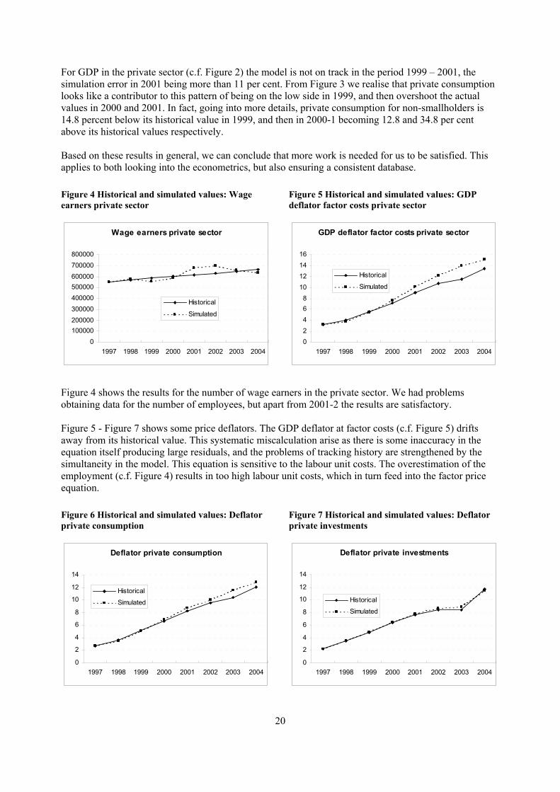
Figure 4 shows the results for the number of wage earners in the private sector. We had problems obtaining data for the number of employees, but apart from 2001-2 the results are satisfactory. Figure 5 - Figure 7 shows some price deflators. The GDP deflator at factor costs (c.f. Figure 5) drifts away from its historical value. This systematic miscalculation arise as there is some inaccuracy in the equation itself producing large residuals, and the problems of tracking history are strengthened by the simultaneity in the model. This equation is sensitive to the labour unit costs. The overestimation of the employment (c.f. Figure 4) results in too high labour unit costs, which in turn feed into the factor price equation. Figure 6 Historical and simulated values: Deflator private consumption

Deflator private consumption

0

2

4

6

8

10

12

14

1997 1998 1999 2000 2001 2002 2003 2004

Historical

Simulated

Figure 7 Historical and simulated values: Deflator private investments

Deflator private investments

0

2

4

6

8

10

12

14

1997 1998 1999 2000 2001 2002 2003 2004

Historical

Simulated

21

The simulation inaccuracy in the GDP deflator at factor cost is directly linked to the private sector GDP deflator at market prices. This in turn, determines the deflator for private consumption, shown in Figure 6, resulting in the same pattern of overestimation. The deflator for private investments (see Figure 7) is not affected by the GDP factor price and labour unit costs, but is a function of the import price, which is exogenous to the model.

6. Multiplier analyses In this section we shall illustrate how the model behaves quantitatively when subjected to two shifts. We have created a baseline simulation extending from 2004 (the final year of the historical database at present) to 2011. This baseline is quite smooth in terms of economic development (see chapter 4 above). In our simulations we first study the effects of a fiscal shift, where we have implemented a permanent increase in government purchases of goods and services (MG) by 10 per cent from 2005 to 2011. In the second simulation we increase the price of imports by 10 per cent from 2005 to 2011.

6.1. Increase in government spending The increase in MG will feed directly into government consumption, increasing it by almost 4.8 per cent (see Figure 8). The increased demand is met by higher domestic production and imports. There will be an immediate increase in the demand component (DEM), which increases imports by about 2 per cent in the long run. Private sector GDP increases by 0.8 per cent the first year and to 1.2 per cent after 7 years. This increase in GDP brings along a rise in operating surplus and wage income (see Figure 9) that lead to higher disposable income and non-smallholders consumption. The increase in demand and private sector GDP cause an increase in the number of wage earners in the private sector. Since the labour force and government employment are exogenous, the number of self-employed is falling, i.e. surplus of labour from (mainly) agriculture is employed in the formal sector.

Figure 8 GDP, consumption, imports. Per cent deviation from baseline scenario

0

1

2

3

4

5

2004 2005 2006 2007 2008 2009 2010 2011

Government consumption Imports

non-Smallholder consumption Private sector GDP

Figure 9 Employment and labour costs. Per cent deviation from baseline scenario

-1

0

1

2

3

4

2004 2005 2006 2007 2008 2009 2010 2011

Labor unit costs Wage earners private sector

Self employed Wage income households

The increase in government consumption will lead to higher government expenditures (see Figure 10), increasing 2.2 per cent the first year. Also revenues increase due to income from direct taxes and taxes on international trade. In Figure 11 we see that government savings as share of current GDP drops 0.68 percentage points (from 3.3 to 2.6), then stabilising at this difference. The government budget deficit is financed solely from domestic borrowing, resulting in increased government interest payments.

22

Increasing private foreign debt finances the current accounts deficit, as government lending abroad is exogenous. We also see that the trade balance and the current accounts are shifted downwards about 0.4 percentage points. Figure 10 Government revenues and expenditures. Per cent deviation from baseline scenario

0

1

2

3

4

2004 2005 2006 2007 2008 2009 2010 2011

Revenue Expenditure

Figure 11 Current accounts and government savings (share of GDP) p.p. deviation from baseline scenario

-0.8

-0.7

-0.6

-0.5

-0.4

-0.3

-0.2

-0.1

0.0

2004 2005 2006 2007 2008 2009 2010 2011

Current accounts Trade balance Government savings

In Figure 12 we show the effects on some of the price deflators in the model. The principal driving forces of the price deflators are import prices and labour costs. Import price is exogenous in the model and the baseline assumptions are presented in Table 3. The J-shaped development occurs because the labour costs declines the first year (see Figure 9) due to non-smallholder GDP (YPFO) increasing more than the wage costs. Private sector wage rate being virtually exogenous the adjustment in labour cost comes entirely from increased employment. In the long run however, labour costs follows the number of employees and the non-smallholders value added. Also the deflator for GDP at factor costs (PYPF) is important to the nominal picture. This deflator depends on import price and labour unit costs (weights of about 2/3 and 1/3 respectively in the long run). Figure 12 Price deflators Per cent deviation from baseline scenario

-0.2

0.0

0.2

0.4

0.6

0.8

1.0

2004 2005 2006 2007 2008 2009 2010 2011

Private consumption Export Private GDP

23

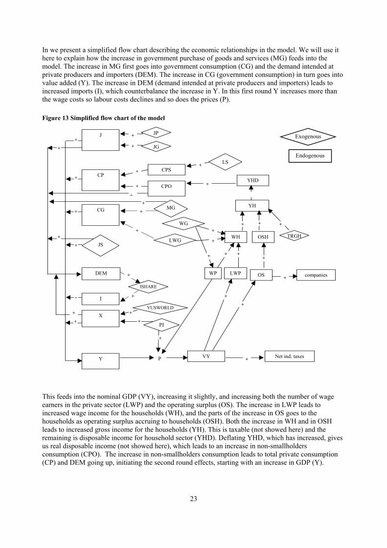
In we present a simplified flow chart describing the economic relationships in the model. We will use it here to explain how the increase in government purchase of goods and services (MG) feeds into the model. The increase in MG first goes into government consumption (CG) and the demand intended at private producers and importers (DEM). The increase in CG (government consumption) in turn goes into value added (Y). The increase in DEM (demand intended at private producers and importers) leads to increased imports (I), which counterbalance the increase in Y. In this first round Y increases more than the wage costs so labour costs declines and so does the prices (P). Figure 13 Simplified flow chart of the model

CP CPS

Y

I

J

CG

JS

ISHARE

CPO

VY

DEM

LS

Net ind. taxes

WH

YH

YHD

OSH TRGH

OS

JG

JP

P

MG

LWG

companies WP

Exogenous

Endogenous

+

+

+

+

+

+

+

+

+ + +

X +

-

++

+

+

+

+

+

+

+

+

+

+WG

+

LWP

+ +

+

+

+

+

+

+ YUSWORLD

+

+PI

+

This feeds into the nominal GDP (VY), increasing it slightly, and increasing both the number of wage earners in the private sector (LWP) and the operating surplus (OS). The increase in LWP leads to increased wage income for the households (WH), and the parts of the increase in OS goes to the households as operating surplus accruing to households (OSH). Both the increase in WH and in OSH leads to increased gross income for the households (YH). This is taxable (not showed here) and the remaining is disposable income for household sector (YHD). Deflating YHD, which has increased, gives us real disposable income (not showed here), which leads to an increase in non-smallholders consumption (CPO). The increase in non-smallholders consumption leads to total private consumption (CP) and DEM going up, initiating the second round effects, starting with an increase in GDP (Y).

24

6.2. Increase in import price An increase in import price will reduce non-smallholders consumption by more than 4 per cent the first year, ending up at a more than 12 per cent reduction in 2011 (c.f. Figure 14). Both the short term and long term effects are mainly due to reduced real disposable income in the household sector. Real disposable income decreases because the consumer price increases following the increase in the price of imported goods. The consumption function has been designed so that private consumption follows real disposable income in the long run. Import volume is assumed a share of domestic demand, in which non-smallholders consumption constitutes more than 60 per cent. It is the reduction in consumption that leads to the reduced volume of imports by 7 per cent in the long run. Although the isolated effect from lower imports on GDP is positive, this lowers the GDP in the private sector by more than 4 per cent in the long run. In the private sector the amount of labor is linked to output through a Cobb-Douglas production function. From Figure 15 we can see that the number of wage earners goes down by 11 per cent relative to the baseline scenario in the long run. This number is outweighed by an increase in the number of self-employed, which in turn leads to an increase in smallholder’s consumption. In 2005 and 2006 the decline in the number of employees in the private sector is stronger than that in value added, so labor unit costs increases temporarily. After that however, reduction in employment is greater then that of value added (the wage rate is unchanged) and the labor unit costs decreases. The wage income to the households drops with the employment in the private sector. Figure 14 GDP, consumption, imports. Per cent deviation from baseline scenario

-13-12-11-10-9-8-7-6-5-4-3-2-10

2004 2005 2006 2007 2008 2009 2010 2011

Imports non-Smallholder consumption Private sector GDP

Figure 15 Employment and labour costs. Per cent deviation from baseline scenario

-12-11-10-9-8-7-6-5-4-3-2-101234

2004 2005 2006 2007 2008 2009 2010 2011

Labor unit costs Wage earners private sector

Self employed Wage income households

In Figure 16 we see that there is an increase in nominal tax revenues the first 5 years. Thereafter tax revenues are lower than in the baseline scenario. The government revenues are affected by the increase in import prices and taxes on international trade (import duties), value added tax and direct taxes on households. Import duties are based on the value of imports, which increases in the whole period, though somewhat less in the long run. The value of import increases by 7.4 per cent the first year, thereafter gradually declining to 2.2 per cent in 2011. It is only when the volume of imports has declined enough to offset the effects from the import duties that total tax revenues goes down. The value added tax is based on the value of consumption. As is evident from Figure 14 and Figure 18 the volume is decreasing while the price increases. The value of consumption, the “tax base”, increases until 2008 (including), thereafter declining. The government income from direct taxes on households follow the same pattern as the value added tax. It first increases before it gradually becomes less than in the baseline scenario. The reduction in the employment (c.f. Figure 15) and the increase in nominal GDP (over the period 2005-10) leads to an

25

increase in the operating surplus. This in turn, leads to an increase in the gross income in the household sector, which is the tax base for direct taxes on the households.

Figure 16 Government revenues and expenditures. Per cent deviation from baseline scenario

-5

-4

-3

-2

-1

0

1

2

3

4

5

6

2004 2005 2006 2007 2008 2009 2010 2011

Revenue Expenditure

Figure 17 Current account and government savings. (Share of GDP) p.p. deviation from baseline scenario

-2.0

-1.5

-1.0

-0.5

0.0

0.5

1.0

2004 2005 2006 2007 2008 2009 2010 2011

Current accounts Trade balance Government savings

The government depends upon imports both for consumption and investments, so the increase in import price will affect their spending. The increase in government expenditures comes from increases in investments and consumption, and is financed by increasing the domestic debt, leading to increased interest payment on the government domestic debt. The increase in expenditures is solely due to increases in prices on investments and consumption, leaving the quantities unchanged. In Figure 18 we see the effects on some of the price indices. Note that the price deflator for private investment is closely related to the (shift in) import price, because of the high import share of investment goods. The other price indices are influenced by the domestic prices, which in turn is linked to the costs of domestic production (labour unit costs).

Figure 18 Price deflators. Per cent deviation from baseline scenario

0.0

2.0

4.0

6.0

8.0

10.0

2004 2005 2006 2007 2008 2009 2010 2011

Private consumption Export

Private GDP Private investment

26

References Malawi Government. Ministry of Economic Planning and Development: Mid-Year Economic Review, July-December 2004. National Statistical Office of Malawi: Various tables and websites (http://www.nso.malawi.net/). Musila, J.W. (2001), An econometric model of the Malawian economy, Economic Modelling 19, 295-330. Reserve Bank of Malawi (2005): Financial and Economic Review, Volume 37, Number 2, 2005.

27

Appendix 1. List of variables Type N = endogenous, X = exogenous Symbol Type Explanation

C N Total consumption

CA N Current account

CG N Government consumption

CP N Private consumption

CPO N Private consumption non smallholders

CPS N Private consumption smallholders

DELTAG X Depreciation rate government capital

DELTAP X Depreciation rate private sector capital

DEM N Demand facing private producers and importers

DG N Depreciation government capital

DP N Depreciation private sector capital

DUM94 X Dummy = 1 in 1994, otherwise = 0

DUM9403 X Dummy = 1 in 1994 and 2003, otherwise = 0

DUM9498 X Dummy = 1 in 1994 and 1998, otherwise = 0

ERROM X Errors and omissions (in capital balance)

FER X Foreign exchange reserves

GEXP N Government expenditures (current accounts)

GREV N Total government revenue

GRTOT N Total government revenue including grants

GSAV N Government saving

HSAV N Household saving

I N Total imports of goods and services

INTFER N Interest payment on foreign exchange reserves

INTG N Interest payment on government debt (domestic and foreign)

INTGD N Interest payment on government domestic debt

INTGF N Interest payment on government debt to foreigners

INTPF N Interest payment on private debt to foreigners

IRFER X Interest rate earned on foreign exchange reserves

IRGD X Interest rate on government domestic debt

IRGF X Interest rate on government foreign debt

IRPF X Interest rate on private debt to foreigners

ISHARE X Share of imports in total demand

J N Total gross investment in fixed capital

JG X Gross investment government sector

JP X Gross investment private sector

JS X Stock building

K N Total stock of fixed capital

KG N Stock of fixed capital government sector

KP N Stock of fixed capital private sector

LABFORCE X Total labour force

LD N Total domestic credit

LDG X Domestic debt to the government

LGD N Domestic government debt

LGF X Government foreign debt

LPD X Private domestic debt

LPF N Private foreign debt

28

LS N Number of self employed

LUC N Labour unit costs

LWG X Number of wage earners government sector

LWP N Number of wage earners private sector

M N Money stock

MG X Government purchase of goods and services (1994-prices)

NFS N Net financial services

NTRFP X Net transfers to private from abroad

OEG X Other expenditures government

ONTR X Other non-tax revenue

OS N Operating surplus

OSH N Operating surplus accruing to households

OSHRATE X Share of operating surplus accruing to households

PCP N Deflator private consumption

PCPO N Deflator private consumption smallholder

PCPS N Deflator private consumption other

PI X Import deflator

PJG N Deflator government investment in fixed capital

PJP N Deflator private investment in fixed capital

PJS N Deflator stockbuilding

PMG N Deflator government purchases of goods and services

PX N Export deflator

PY N GDP-deflator

PYFAG N Deflator GDP agricultural sector in factor prices

PYFAGL N Deflator GDP agricultural large scale sector in factor prices

PYFAGS N Deflator GDP agricultural small scale sector in factor prices

PYFCO N Deflator GDP construction sector in factor prices

PYFDI N Deflator GDP distribution sector in factor prices

PYFEW N Deflator GDP electricity and water sector in factor prices

PYFFP N Deflator GDP financial and professional sector in factor prices

PYFMA N Deflator GDP manufacturing sector in factor prices

PYFMQ N Deflator GDP mining and quarrying sector in factor prices

PYFOD N Deflator GDP ownership of dwelling sector in factor prices

PYFPS N Deflator GDP priv. and social com. services sector in factor prices

PYFSE N Deflator GDP services sector in factor prices

PYFTC N Deflator GDP transport and communication sector in factor prices

PYFUC N Deflator GDP agricultural sector in factor prices

PYP N Deflator GDP private sector in market prices

PYPF N Deflator GDP private sector in factor prices

RCG X Residual government consumption

RCPO X Residual consumption non smallholders sector

RCPS X Residual consumption smallholders sector

RLWP X Residual labour demand

RNFS X Residual net factor services

ROSH X Residual operating surplus to households

RPCPO X Residual deflator non smallholders sector

RPCPS X Residual deflator smallholders sector

RPJP X Residual deflator for private investment

RPJS X Residual deflator for stockbuilding

RPMG X Residual deflator for government purchases of goods

RPX X Residual deflator for exports

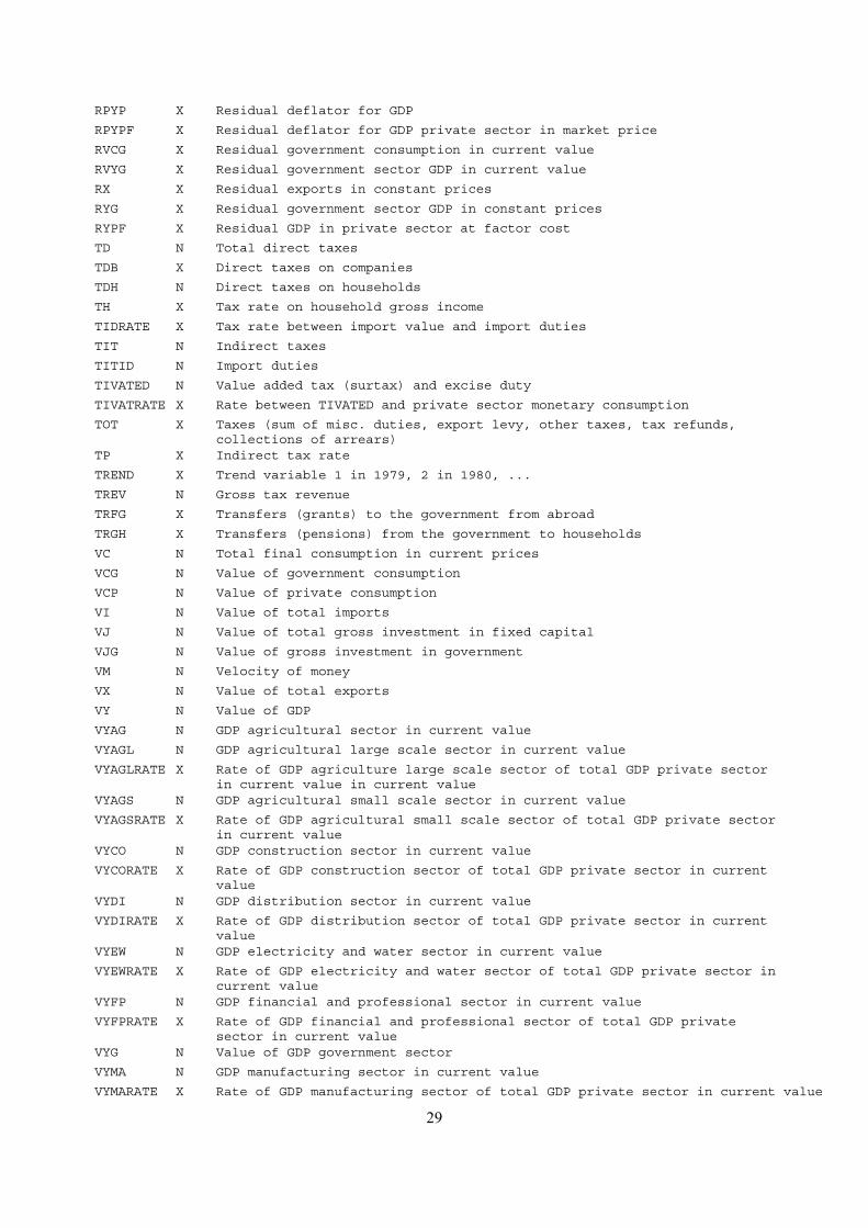
29

RPYP X Residual deflator for GDP

RPYPF X Residual deflator for GDP private sector in market price

RVCG X Residual government consumption in current value

RVYG X Residual government sector GDP in current value

RX X Residual exports in constant prices

RYG X Residual government sector GDP in constant prices

RYPF X Residual GDP in private sector at factor cost

TD N Total direct taxes

TDB X Direct taxes on companies

TDH N Direct taxes on households

TH X Tax rate on household gross income

TIDRATE X Tax rate between import value and import duties

TIT N Indirect taxes

TITID N Import duties

TIVATED N Value added tax (surtax) and excise duty

TIVATRATE X Rate between TIVATED and private sector monetary consumption

TOT X Taxes (sum of misc. duties, export levy, other taxes, tax refunds, collections of arrears)

TP X Indirect tax rate

TREND X Trend variable 1 in 1979, 2 in 1980, ...

TREV N Gross tax revenue

TRFG X Transfers (grants) to the government from abroad

TRGH X Transfers (pensions) from the government to households

VC N Total final consumption in current prices

VCG N Value of government consumption

VCP N Value of private consumption

VI N Value of total imports

VJ N Value of total gross investment in fixed capital

VJG N Value of gross investment in government

VM N Velocity of money

VX N Value of total exports

VY N Value of GDP

VYAG N GDP agricultural sector in current value

VYAGL N GDP agricultural large scale sector in current value

VYAGLRATE X Rate of GDP agriculture large scale sector of total GDP private sector in current value in current value

VYAGS N GDP agricultural small scale sector in current value

VYAGSRATE X Rate of GDP agricultural small scale sector of total GDP private sector in current value

VYCO N GDP construction sector in current value

VYCORATE X Rate of GDP construction sector of total GDP private sector in current value

VYDI N GDP distribution sector in current value

VYDIRATE X Rate of GDP distribution sector of total GDP private sector in current value

VYEW N GDP electricity and water sector in current value

VYEWRATE X Rate of GDP electricity and water sector of total GDP private sector in current value

VYFP N GDP financial and professional sector in current value

VYFPRATE X Rate of GDP financial and professional sector of total GDP private sector in current value

VYG N Value of GDP government sector

VYMA N GDP manufacturing sector in current value

VYMARATE X Rate of GDP manufacturing sector of total GDP private sector in current value

30

VYMQ N GDP mining and quarrying sector in current value

VYMQRATE X Rate of GDP mining and quarrying sector of total GDP private sector in current value

VYOD N GDP ownership of dwelling sector of total GDP private sector in current value

VYODRATE X Rate of GDP ownership of dwelling sector of total GDP private sector in current value

VYP N Value of private sector GDP

VYPS N GDP private and social community services sector in current value

VYPSRATE X Rate of GDP private and social community services sector of total GDP private sector in current value

VYSE N GDP services sector in current value

VYTC N GDP transport and communication sector in current value

VYTCRATE X Rate of GDP transport and communication sector of total GDP private sector in current value

VYUC N GDP unallocable finance charges sector in current value

WG X Wage rate government sector employees

WH N Total wage income for households

WP N Wage rate private sector employees

X N Volume of total exports

Y N GDP in constant 1994-prices

YF N GDP at 1994 factor cost

YFAG N GDP agricultural scale sector at constant 1994 factor cost

YFAGL N GDP agricultural large scale sector at constant 1994 factor cost

YFAGLRATE X Rate of GDP agricultural large scale sector of total GDP private sector at constant 1994 factor cost

YFAGS N GDP agricultural small scale sector at constant 1994 factor cost

YFAGSRATE X Rate of GDP agricultural small scale sector of total GDP private sector at constant 1994 factor cost

YFCO N GDP construction sector at constant 1994 factor cost

YFCORATE X Rate of GDP construction sector of total GDP private sector at constant 1994 factor cost

YFDI N GDP distribution sector at constant 1994 factor cost

YFDIRATE X Rate of GDP distribution sector of total GDP private sector at constant 1994 factor cost

YFEW N GDP electricity and water sector at constant 1994 factor cost

YFEWRATE X Rate of GDP electricity and water sector of total GDP private sector at constant 1994 factor cost

YFFP N GDP financial and professional sector at constant 1994 factor cost

YFFPRATE X Rate of GDP financial and professional sector of total GDP private sector at constant 1994 factor cost

YFMA N GDP manufacturing sector at constant 1994 factor cost

YFMARATE X Rate of GDP manufacturing sector of total GDP private sector at constant 1994 factor cost

YFMQ N GDP mining and quarrying sector at constant 1994 factor cost

YFMQRATE X Rate of GDP mining and quarrying sector of total GDP private sector at constant 1994 factor cost

YFOD N GDP ownership of dwelling sector at constant 1994 factor cost

YFODRATE X Rate of GDP ownership of dwelling sector of total GDP private sector at constant 1994 factor cost

YFPS N GDP private and social community services sector at constant 1994 factor cost

YFPSRATE X Rate of GDP private and social community services sector of total GDP private sector at constant 1994 factor cost

YFSE N GDP services sector at constant 1994 factor cost

YFTC N GDP transport and communication sector at constant 1994 factor cost

YFTCRATE X Rate of GDP transport and communication sector of total GDP private sector at constant 1994 factor cost

YFUC N GDP unallocable finance charges sector at constant 1994 factor cost

31

YG N GDP in government sector in 1994-prices

YH N Gross income household sector

YHD N Disposable income household sector

YHDR N Real disposable income household sector

YP N GDP in fixed 1994-market prices, private sector

YPF N GDP in fixed 1994-factor prices, private sector

YPFO N GDP in fixed 1994-factor prices, private sector non smallholder sector

YUSWORLD X GDP World

32

Appendix 2. Some data issues Most of the data used in the model are taken directly from the national accounts of Malawi. As in the current Malawian National Accounts the base year in the model is 1994 implying that values in fixed and current prices are equal in that year. Thus all price indices are equal to unity in 1994. Malawian data for some important variables do not exist and have to be estimated for each year. In what follows we will describe how this was done.

Appendix 2.1. Capital stocks The national accounts do not include capital stock estimates. We have used the standard perpetual inventory method. First we have looked at the series for gross investment in fixed capital by sector (private and government). For the private sector gross investment (JP) is a stationary variable although it fluctuates a lot. We thus estimated the average investment over the entire period 1979 to 2002 and divided it by an assumed depreciation rate (set to 0.1) in order to get an estimate of the initial capital stock KP(0) where year 0 is the end of 1978. Then assuming the equations included in the model, a series of capital stock data can easily be estimated. For the government sector we have used the same method. In this case, however, the investment series are not necessarily stationary (a formal test has not been carried out). There is a high investment level in the early years dropping to about half the level in the early 1980s before increasing back to initial levels during the later 1990s. Thus it is far from obvious how to chose a representative and "stationary" level. We have simply chosen the average investment level again using data for the period 1979 to 2002. Then calculated the initial capital stock as explained above using the same depreciation rate as for the private sector. Then the formulas in the model handle the rest. Note however, that the data for depreciation and capital stock in the government sector is not really used for anything in the model as it now stands as capital costs is not included in the construction of government consumption and value added. Also since we are mainly interested in the period starting in the mid 1990s and onwards, the importance of our guesstimate of the initial capital stock diminishes quite quickly when the assumed depreciation rate is as high as 0.1. Thus the capital stock in the latter part of our historical period is not very sensitive to our initial estimate.

Appendix 2.2. Employment We have data for employment of wage earners (employees) from 1979 to 1995, but not for more recent years. The data for employees in the government sector (LWG) are extended assuming virtually no change in government employment from 1995 to 2003. We have the wage sum (wages and salaries in government sector) from the national accounts. Thus given WG*LWG and our estimate for LWG, we calculate WG. To determine private sector employment of wage earners a more elaborate procedure has been used. Using the postulated Cobb-Douglas production function and using first order conditions for profit maximization, we now that the share of wages in factor income is equal to the parameter α in the production function. We use data for the period where data do exist, to estimate α. Using this estimate for years after 1995 together with data for factor income in current prices, we can calculate the sum of wages and salaries in the private sector (WP*LWP). We then assumed a constant ratio between government and private wage rates per employee in order to get an estimate of WP. Then LWP can be calculated. This procedure gave unreasonably large fluctuations in LWP, so the initial estimate was somewhat smoothed (using a centred moving average) to produce the final estimate of LWP. Given this smoothing procedure, the initial estimate of WP*LWP is changed due to changes in LWP so that the factor share has a cyclical development as opposed to the constant level chosen initially using the production function parameter.

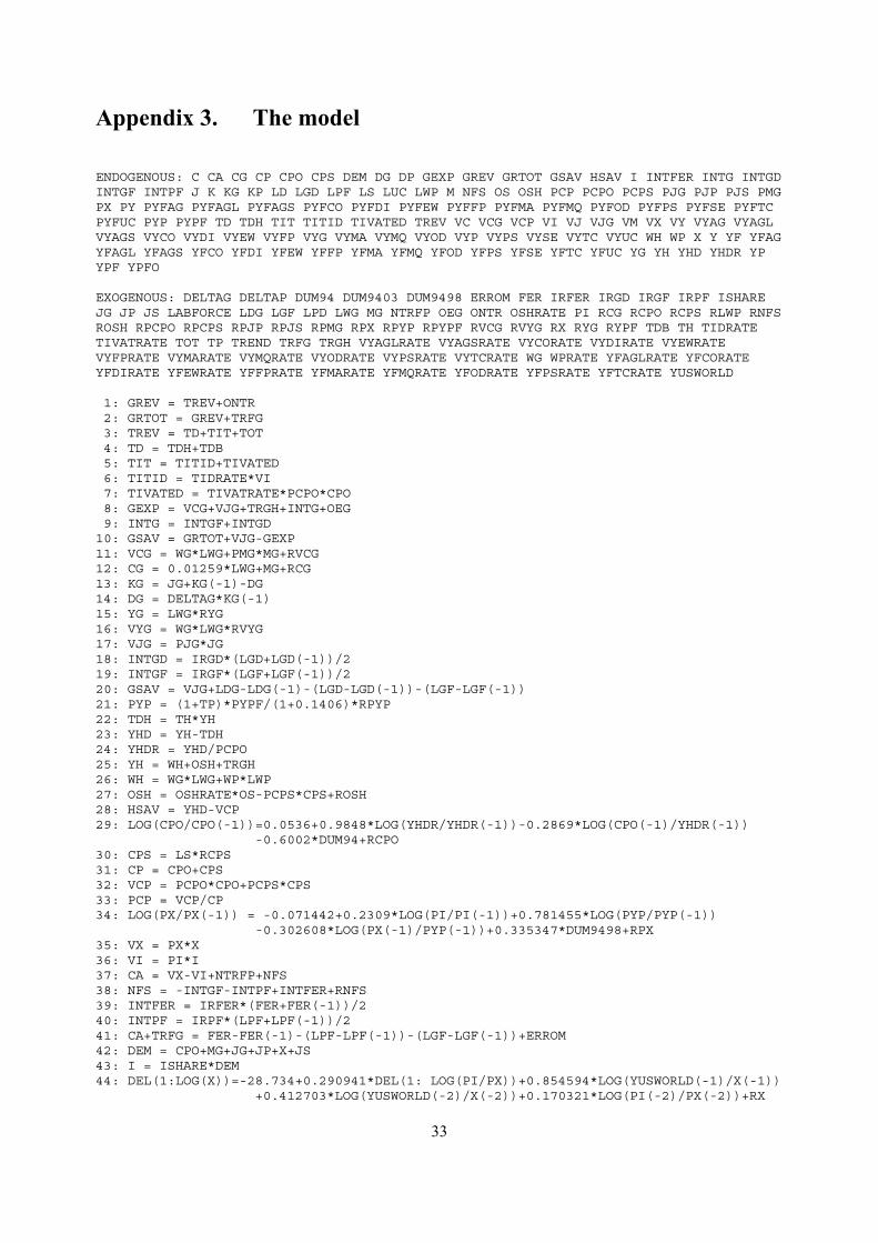
33

Appendix 3. The model ENDOGENOUS: C CA CG CP CPO CPS DEM DG DP GEXP GREV GRTOT GSAV HSAV I INTFER INTG INTGD INTGF INTPF J K KG KP LD LGD LPF LS LUC LWP M NFS OS OSH PCP PCPO PCPS PJG PJP PJS PMG PX PY PYFAG PYFAGL PYFAGS PYFCO PYFDI PYFEW PYFFP PYFMA PYFMQ PYFOD PYFPS PYFSE PYFTC PYFUC PYP PYPF TD TDH TIT TITID TIVATED TREV VC VCG VCP VI VJ VJG VM VX VY VYAG VYAGL VYAGS VYCO VYDI VYEW VYFP VYG VYMA VYMQ VYOD VYP VYPS VYSE VYTC VYUC WH WP X Y YF YFAG YFAGL YFAGS YFCO YFDI YFEW YFFP YFMA YFMQ YFOD YFPS YFSE YFTC YFUC YG YH YHD YHDR YP YPF YPFO EXOGENOUS: DELTAG DELTAP DUM94 DUM9403 DUM9498 ERROM FER IRFER IRGD IRGF IRPF ISHARE JG JP JS LABFORCE LDG LGF LPD LWG MG NTRFP OEG ONTR OSHRATE PI RCG RCPO RCPS RLWP RNFS ROSH RPCPO RPCPS RPJP RPJS RPMG RPX RPYP RPYPF RVCG RVYG RX RYG RYPF TDB TH TIDRATE TIVATRATE TOT TP TREND TRFG TRGH VYAGLRATE VYAGSRATE VYCORATE VYDIRATE VYEWRATE VYFPRATE VYMARATE VYMQRATE VYODRATE VYPSRATE VYTCRATE WG WPRATE YFAGLRATE YFCORATE YFDIRATE YFEWRATE YFFPRATE YFMARATE YFMQRATE YFODRATE YFPSRATE YFTCRATE YUSWORLD 1: GREV = TREV+ONTR 2: GRTOT = GREV+TRFG 3: TREV = TD+TIT+TOT 4: TD = TDH+TDB 5: TIT = TITID+TIVATED 6: TITID = TIDRATE*VI 7: TIVATED = TIVATRATE*PCPO*CPO 8: GEXP = VCG+VJG+TRGH+INTG+OEG 9: INTG = INTGF+INTGD 10: GSAV = GRTOT+VJG-GEXP 11: VCG = WG*LWG+PMG*MG+RVCG 12: CG = 0.01259*LWG+MG+RCG 13: KG = JG+KG(-1)-DG 14: DG = DELTAG*KG(-1) 15: YG = LWG*RYG 16: VYG = WG*LWG*RVYG 17: VJG = PJG*JG 18: INTGD = IRGD*(LGD+LGD(-1))/2 19: INTGF = IRGF*(LGF+LGF(-1))/2 20: GSAV = VJG+LDG-LDG(-1)-(LGD-LGD(-1))-(LGF-LGF(-1)) 21: PYP = (1+TP)*PYPF/(1+0.1406)*RPYP 22: TDH = TH*YH 23: YHD = YH-TDH 24: YHDR = YHD/PCPO 25: YH = WH+OSH+TRGH 26: WH = WG*LWG+WP*LWP 27: OSH = OSHRATE*OS-PCPS*CPS+ROSH 28: HSAV = YHD-VCP 29: LOG(CPO/CPO(-1))=0.0536+0.9848*LOG(YHDR/YHDR(-1))-0.2869*LOG(CPO(-1)/YHDR(-1))

-0.6002*DUM94+RCPO 30: CPS = LS*RCPS 31: CP = CPO+CPS 32: VCP = PCPO*CPO+PCPS*CPS 33: PCP = VCP/CP 34: LOG(PX/PX(-1)) = -0.071442+0.2309*LOG(PI/PI(-1))+0.781455*LOG(PYP/PYP(-1))

-0.302608*LOG(PX(-1)/PYP(-1))+0.335347*DUM9498+RPX 35: VX = PX*X 36: VI = PI*I 37: CA = VX-VI+NTRFP+NFS 38: NFS = -INTGF-INTPF+INTFER+RNFS 39: INTFER = IRFER*(FER+FER(-1))/2 40: INTPF = IRPF*(LPF+LPF(-1))/2 41: CA+TRFG = FER-FER(-1)-(LPF-LPF(-1))-(LGF-LGF(-1))+ERROM 42: DEM = CPO+MG+JG+JP+X+JS 43: I = ISHARE*DEM 44: DEL(1:LOG(X))=-28.734+0.290941*DEL(1: LOG(PI/PX))+0.854594*LOG(YUSWORLD(-1)/X(-1))

+0.412703*LOG(YUSWORLD(-2)/X(-2))+0.170321*LOG(PI(-2)/PX(-2))+RX

34

45: DEL(1:LOG(LWP)) = 2.0578+0.4321*DEL(1: LOG(YPFO))-0.4586*(LOG(LWP(-1)) -2*LOG(YPFO(-1))+LOG(KP(-2)))-0.0101*TREND+RLWP

46: KP = JP-DP+KP(-1) 47: DP = DELTAP*KP(-1) 48: OS = PYPF*YPF-WP*LWP 49: YPF = YPFO+YFAGS 50: LUC = WP*LWP/YPFO 51: LOG(PYPF/PYPF(-1)) = 0.104321+0.708408*LOG(PYPF(-1)/PYPF(-2))+

0.475095*LOG(PI/PI(-1))+0.235742*LOG(LUC/LUC(-1)) -0.364528*LOG(PYPF(-1)/PI(-1))+0.146252*LOG(LUC(-1)/PI(-1))+RPYPF

52: LOG(PCPO/PCPO(-1)) = 0.052753+0.286583*LOG(PI/PI(-1))+0.613581*LOG(PYP/PYP(-1)) -0.531505*LOG(PCPO(-1)/PI(-1))+0.236691*LOG(PYP(-1)/PI(-1))+RPCPO

53: LOG(PJP/PJP(-1)) = 0.102279+0.810991*LOG(PI/PI(-1))-0.5266*LOG(PJP(-1)/PI(-1)) -0.193706*DUM9403+RPJP

54: PJG = PJP 55: PMG = PYP*RPMG 56: PJS = PYP*RPJS 57: PCPS = PCP*RPCPS 58: Y+I = C+J+JS+X 59: Y = YG+YP 60: C = CG+CP 61: J = JG+JP 62: PY*Y+VI = VCG+VCP+VJ+PJS*JS+VX 63: VY = VYG+VYP 64: VYP = PYP*YP 65: YPF = YP/(1+0.1406)+RYPF 66: VC = VCP+VCG 67: VJ = PJG*JG+PJP*JP 68: K = KG+KP 69: LABFORCE = LWG+LWP+LS 70: WP = WPRATE*WG 71: M = LD+FER 72: LD = LGD-LDG+LPD 73: VM = VY/M 74: YFAGS = CPS 75: YFAGL = YFAGLRATE*YPF 76: YFMQ = YFMQRATE*YPF 77: YFMA = YFMARATE*YPF 78: YFEW = YFEWRATE*YPF 79: YFCO = YFCORATE*YPF 80: YFOD = YFODRATE*YPF 81: YFDI = YFDIRATE*YPF 82: YFTC = YFTCRATE*YPF 83: YFFP = YFFPRATE*YPF 84: YFPS = YFPSRATE*YPF 85: YFUC = YPF-YFAGS-YFAGL-YFMQ-YFMA-YFEW-YFCO-YFOD-YFDI-YFTC-YFFP-YFPS 86: YFAG = YFAGS+YFAGL 87: YFSE = YFDI+YFTC+YFFP+YFPS+YG+YFUC 88: YF = YFAG+YFMQ+YFMA+YFEW+YFCO+YFOD+YFSE 89: VYAGS = VYAGSRATE*VYP 90: VYAGL = VYAGLRATE*VYP 91: VYMQ = VYMQRATE*VYP 92: VYMA = VYMARATE*VYP 93: VYEW = VYEWRATE*VYP 94: VYCO = VYCORATE*VYP 95: VYOD = VYODRATE*VYP 96: VYDI = VYDIRATE*VYP 97: VYTC = VYTCRATE*VYP 98: VYFP = VYFPRATE*VYP 99: VYPS = VYPSRATE*VYP 100: VYUC = VYP-VYAGS-VYAGL-VYMQ-VYMA-VYEW-VYCO-VYOD-VYDI-VYTC-VYFP-VYPS 101: VYAG = VYAGS+VYAGL 102: VYSE = VYDI+VYTC+VYFP+VYPS+VYG+VYUC 103: PYFAGS = VYAGS/YFAGS 104: PYFAGL = VYAGL/YFAGL 105: PYFMQ = VYMQ/YFMQ 106: PYFMA = VYMA/YFMA

35

107: PYFEW = VYEW/YFEW 108: PYFCO = VYCO/YFCO 109: PYFOD = VYOD/YFOD 110: PYFDI = VYDI/YFDI 111: PYFTC = VYTC/YFTC 112: PYFFP = VYFP/YFFP 113: PYFPS = VYPS/YFPS 114: PYFUC = VYUC/YFUC 115: PYFAG = VYAG/YFAG 116: PYFSE = VYSE/YFSE

36

Appendix 4. Estimation results

Appendix 4.1. Introduction The selection of equations for estimation is based on a desirability to cover main parts of the private sector economic behaviour and the availability of data. One obvious candidate is the equation describing private consumption, due to its large contribution to GDP. The equation for volume of exports is also estimated using a so-called Armington function. A labour demand function has been estimated using an inverted Cobb-Douglas production function. In addition we have estimated four price equations; export price, consumer price, factor price and the price of private investments. Our estimation methods have been Ordinary Least Squares (OLS). Some effort has been put into the dynamic specification of the equations. Together with the simultaneous modelling approach for the model as a whole, this should gain the macroeconomic modelling efforts considerably. Building a model concentrating for the most on analysing short to medium terms effects of policy shocks and forecasts, a good description of the dynamic process is needed. Having said that, the dynamic specification of the model requires more effort by the model users to obtain a sound knowledge of the workings of the model than in the case of static equations. The general econometric approach is often named “general to specific”, because we start with a fairly general model including all relevant variables according to economic theory. The econometric specification at this stage should be quite flexible. During the estimation process variables whose coefficients are not considered significant is removed and restrictions are tested and imposed in order to obtain a specification without to many coefficients to estimate. All equations in this section are specified as log-linear, giving the advantage that the elasticities are easily calculated from estimated results. The dynamic specification is the so-called error-correction model in which both the long run properties and short run dynamics can be specified explicitly. When simulating these equations, the error-correction mechanism will force the endogenous variables towards the long run (steady state) solution. In the true economy there will always be short-term shocks pushing the economy outside this steady-state path. The error correction formulation opens up for this shocks and in the same time ensures that the economy is drawn back towards the (more structural) long run solution. One particular advantage with this specification is that it is easy to impose and test theoretical assumptions, and the structural economic theory build into the equation can be read out of the so called error correction term. For a simple two variable model, the log-linear specification can be written as follows: A5 1 log(y)-log(y-1) = a + b*log(y-1) + c*log(x-1) + d*(log(x)-log(x - 1)) + e*log((y - 1)-log(y - 2)) + u

where y is the endogenous variable, x is the exogenous variable, u is the error term and a, b, c, d and e are coefficients. The highlighted part of the equation is the long run solution, while the underlined part is the short run dynamics. The estimate of b should always be negative and the long run elasticity is given by –c/b. If the estimate of c is negative, the elasticity is accordingly positive and vice versa. If estimates c and d are equal, the (long run) elasticity is equal to 1 and the restriction b = c can be imposed explicitly in the equation and tested as in the following regression (where difference terms are omitted for simplicity): A5 2 log(y)-log(y-1) = a + b*(log(y-1) + log(x-1)) + f* log(y-1) + u If f is significant, the restriction b = c is accepted. For a three variable model the restriction will be imposed somewhat differently. For ease of exposition, we omit difference and error terms. The model without restrictions is:

37

A5 3 log(y)-log(y-1) = a + b*log(y-1) + c*log(x-1) + d* log(z-1) The following specification impose the restriction that the sum of the long run elasticities are unity, the elasticity of y with respect to x being c/c+d, and the elasticity with respect to z is equal to d/c+d: A5 4 log(y)-log(y-1) = a + c*(log(y-1) - log(x-1)) + d*(log(y-1) - log(z-1)) Tests of restrictions and the procedure leading from the general to the preferred equation are not presented here, but explanation of the chosen spesification are attached to each equation. The final version of each equation is presented, based on estimation of the implemented equation in TROLL. The most important output from TROLL estimation is as follows: Table 5 Statistics from estimation in TROLL

Output statistics Explanation Output statistics Explanation NOB Number of observations NOVAR Number of variables NOCOEF Number of coefficients RANGE Estimation period RSQ R2 SER Standard error of regression DW Durbin-Watson statistic ESTIMATE Estimated values STER Standard deviation TSTAT T-statistic

Appendix 4.2. Private consumption A typical consumption function would include an income term, a wealth term and a real interest term. Due to weak data we exclude the wealth-term. Due to estimation results we have also discarded the real interest variable from the equation. As the income term we use disposable income in households, adjusted for inflation. The consumption function applies only to households that are not smallholders, and their consumption is called CPO. The equation in the model is LOG(CPO/CPO(-1))=0.0536+0.9848*LOG(YHDR/YHDR(-1))-0.2869*LOG(CPO(-1)/YHDR(-1))

-0.6002*DUM94+RCPO

Symbols in the equation CPO Private consumption non-smallholders YHDR Real disposable income household sector DUM94 Dummy = 1 in 1994, otherwise = 0 RCPO Residual term consumption non-smallholders sector In the short term consumption will rise if the real disposable income is increasing, this is the term 0.9848*LOG(YHDR/YHDR(-1)). If the gap between the level of consumption and real disposable income is negative (i.e. positive saving), that is, if LOG(CPO(-1)/YHDR(-1)) is negative, this is adjusted by increasing the consumption level to its long run level. The fact that the coefficient in the long term is one reflects that consumption in the long run follows the income level. To isolate the long run solution we eliminate all lags and replace all delta terms with zeros. Then we get:

0 = -0.2869*LOG(CPO/YHDR)-0.6002*DUM94, or (removing the dummy)

0.2869*LOG(CPO) = 0.2869*LOG(YHDR), or (dividing and taking anti-log)

CPO = YHDR, which is the long run solution.

38

Figure 19 Actual and fitted values: Non-smallholders consumption

ORDINARY LEAST SQUARES

LHS VARIABLE: LOG(CPO/CPO(-1)) NOB = 23 NOVAR = 4 NCOEF = 4 RANGE: 1982A to 2004A RSQ = 0.45038 CRSQ = 0.363598 F(3/19) = 5.189786 PROB>F = 0.008683 SER = 0.131651 SSR = 0.329306 DW(0) = 1.597949 COND = 2.798646 MAX:HAT = 1 RSTUDENT = NA DFFITS = NA COEF ESTIMATE STER TSTAT PROB>|T| LOG(YHDR/YHDR(-1)) 0.984823 0.268847 3.663136 0.001653 LOG(CPO(-1)/YHDR(-1)) -0.286946 0.149176 -1.923542 0.069527 DUM94 -0.600209 0.193611 -3.100076 0.005894 CONST 0.053583 0.028319 1.892128 0.073814

Appendix 4.3. Price of export The price of exports depends on price of imports, reflecting cost of input factors and world market prices, and the price on domestic value added, reflecting wages and other domestic cost drivers. The export estimated price equation is: LOG(PX/PX(-1)) = -0.0714 + 0.2309*LOG(PI/PI(-1))+0.7814*LOG(PYP/PYP(-1)) -0.3026*LOG(PX(-1)/PYP(-1))+0.3353*DUM9498+RPX

39

Symbols in the equation PX Export deflator PI Import deflator PYP Deflator GDP in the private sector in market prices DUM9498 Dummy = 1 in 1994 and 1998, otherwise = 0 RPX Residual term deflator for exports From the long run version of this equation, given as 0 = -0.302608*LOG(PX/PYP)+0.335347*DUM9498

we realise that in the long run export prices follow the price on domestic value added. In the short run export prices will increase as the import and/or value added prices increases. Figure 20 Actual and fitted values: Export price

ORDINARY LEAST SQUARES LHS VARIABLE: LOG(PX/PX(-1)) NOB = 24 NOVAR = 5 NCOEF = 5 RANGE: 1981A to 2004A RSQ = 0.79274 CRSQ = 0.749106 F(4/19) = 18.168057 PROB>F = 0 SER = 0.095838 SSR = 0.174513 DW(0) = 1.913695 COND = 7.176143 MAX:HAT = 0.68038 RSTUDENT = -2.27693 DFFITS = 2.668272 COEF ESTIMATE STER TSTAT PROB>|T| LOG(PI/PI(-1)) 0.226913 0.167065 1.358232 0.190301 LOG(PYP/PYP(-1)) 0.785573 0.203952 3.851759 0.001075

40

LOG(PX(-1)/PYP(-1)) -0.297663 0.161375 -1.844541 0.080753 DUM9498 0.337171 0.08596 3.92242 0.000915 CONST -0.070908 0.06036 -1.174751 0.254608

Appendix 4.4. Volume of exports We have estimated an export equation of the so-called Armington type (exports depend on relative prices between domestic export prices and world market prices, as well as an indicator of markets size or market growth. The estimated function is DEL(LOG(X)) = -28.734 + 0.2909*DEL(1: LOG(PI/PX))+0.8545*LOG(YUSWORLD(-1)/X(-1))

+0.4127*LOG(YUSWORLD(-2)/X(-2))+0.1703*LOG(PI(-2)/PX(-2))+RX

Symbols in the equation X Volume of total exports YUSWORLD GDP World PI Import deflator PX Export deflator In the short run, exports increase if imports get relatively more expensive than exports, i.e. if PI increases more than PX, which means Malawian goods are increasing their market share on the world market. In the long run, exports will grow at the same speed as the world market size, for given relative prices. If Malawian exports become relatively cheaper than other countries exports, exports from Malawi will grow faster than the world market, and gain market share. This is clear from studying the long run part of the equation, given as 0 = 0.854594*LOG(YUSWORLD/X)+0.412703*LOG(YUSWORLD/X)+0.170321*LOG(PI/PX)

or, LOG(X) = LOG(YUSWORLD) + (0.1703/1.2672)*[LOG(PI)- LOG (PX)]

41

Figure 21 Actual and fitted values: Volume of exports

ORDINARY LEAST SQUARES LHS VARIABLE: DEL(1: LOG(X)) NOB = 24 NOVAR = 5 NCOEF = 5 RANGE: 1981A to 2004A RSQ = 0.673979 CRSQ = 0.605343 F(4/19) = 9.819625 PROB>F = 0.000176 SER = 0.082183 SSR = 0.128327 DW(0) = 1.5545 COND = 712.45195 MAX:HAT = 0.608422 RSTUDENT = -2.136748 DFFITS = 0.797582 COEF ESTIMATE STER TSTAT PROB>|T| DEL(1: LOG(PI/PX)) 0.289729 0.112437 2.576804 0.018476 LOG(YUSWORLD(-1)/X(-1)) 0.85468 0.1642 5.205109 5.03739239e-005 LOG(YUSWORLD(-2)/X(-2)) 0.411276 0.178479 2.304343 0.03266 LOG(PI(-2)/PX(-2)) 0.170506 0.067115 2.540513 0.019956 CONST -28.703678 5.401225 -5.31429 3.95803661e-005

Appendix 4.5. Private sector employment We have modeled private sector employment by the following equation: DEL(1: LOG(LWP)) = 2.0578+0.4321*DEL(1: LOG(YPFO))-0.4586*(LOG(LWP(-1)) -2*LOG(YPFO(-1))

+ LOG(KP(-2)))-0.0101*TREND+RLWP

Symbols in the equation LWP Number of wage earners in the private sector

42

YPFO GDP in fixed 1994-factor prices, private sector non-smallholder sector KP Stock of fixed capital in the private sector TREND Trend variable 1 in 1979, 2 in 1980, etc. RLWP Residual term number of wage earners in the private sector It is an inverted production function, and the change in labour employed is determined by the change in value added, the level of employment relative to value added and capital, and a trend variable. In the short run labour demand is only affected by changes in output. In the long run we have the following relationship: 0 = -0.4586*(LOG(LWP)-2*LOG(YPFO)+LOG(KP))-0.0101*TREND

where the specification of the long run solution LOG(LWP) = 2*LOG(YPFO)+LOG(KP), implies that we have imposed constant returns to scale and the labour and capital share is set to 0.5. This assumption is roughly in line with tests and results from the estimation process. Note that the trend variable is the same as an inverted total factor productivity-factor. The error correction mechanism of the equation can be written as YPFO = e0.11TREND * LWP0.5 * KP0.5

Figure 22 Actual and fitted values: Number of wage earners, private sector

ORDINARY LEAST SQUARES LHS VARIABLE: DEL(1: LOG(LWP)) NOB = 23 NOVAR = 4 NCOEF = 4 RANGE: 1982A to 2004A RSQ = 0.460683 CRSQ = 0.375527 F(3/19) = 5.409911 PROB>F = 0.007322

43

SER = 0.052963 SSR = 0.053296 DW(0) = 2.680604 COND = 130.089647 MAX:HAT = 0.482737 RSTUDENT = 3.213222 DFFITS = 1.344543 COEF ESTIMATE STER TSTAT PROB>|T| DEL(1: LOG(YPFO)) 0.468785 0.217879 2.151584 0.044504 LOG(LWP(-1)) -0.49184 0.132586 -3.709585 0.001487 -2*LOG(YPFO(-1)) +LOG(KP(-2)) TREND -0.011944 0.003353 -3.562346 0.002079 CONST 2.225925 0.587017 3.791929 0.001232

Appendix 4.6. Factor price The equation for value added at factor prices is estimated as: LOG(PYPF/PYPF(-1)) = 0.104321+0.708408*LOG(PYPF(-1)/PYPF(-2))+

0.475095*LOG(PI/PI(-1))+0.235742*LOG(LUC/LUC(-1)) -0.364528*LOG(PYPF(-1)/PI(-1))+0.146252*LOG(LUC(-1)/PI(-1)) +RPYPF

Symbols in the equation PYPF Deflator GDP in the private sector in factor prices PI Import deflator LUC Labour unit costs RPYPF Residual term deflator for GDP in the private sector at factor cost In the short run, changes in PYPF are given by changes in labour unit costs and changes in import prices. The inclusion of change in PYPF with one lag on the right hand side reflects some persistence in these prices. In the long run, PYPF is positively affected by import prices, reflecting partly that some inputs are imported and partly that domestic products to some extent compete with internationally produced products. Secondly, PYPF is positively affected by labour unit costs, mirroring that producers must cover increased wage costs by increasing their prices on produced goods. In the long run we have LOG(PYPF) = 0.598790*LOG(PI)+ 0.401209*LOG(LUC)

44

Figure 23 Actual and fitted values: Factor price deflator, GDP private sector

ORDINARY LEAST SQUARES LHS VARIABLE: LOG(PYPF/PYPF(-1)) NOB = 23 NOVAR = 6 NCOEF = 6 RANGE: 1982A to 2004A RSQ = 0.791617 CRSQ = 0.730328 F(5/17) = 12.916105 PROB>F = 0 SER = 0.065226 SSR = 0.072326 DW(0) = 2.435739 COND = 15.802914 MAX:HAT = 0.825065 RSTUDENT = 2.249119 DFFITS = 2.381552 COEF ESTIMATE STER TSTAT PROB>|T| LOG(PYPF(-1)/PYPF(-2)) 0.703712 0.119244 5.901457 1.74119835e-005 LOG(PI/PI(-1)) 0.495126 0.103012 4.806474 0.000165 LOG(LUC/LUC(-1)) 0.183297 0.085492 2.144021 0.046783 LOG(PYPF(-1)/PI(-1)) -0.368342 0.097561 -3.775496 0.001509 LOG(LUC(-1)/PI(-1)) 0.112088 0.065132 1.720935 0.10341 CONST 0.073053 0.075288 0.97032 0.345491

Appendix 4.7. Consumer price The deflator for private, non-smallholders consumption is estimated as a function of prices on domestically and foreign produced goods, reflecting that both type of goods are included in the consumption basket. The equation is: LOG(PCPO/PCPO(-1)) = 0.052753+0.286583*LOG(PI/PI(-1))+0.613581*LOG(PYP/PYP(-1))

-0.531505*LOG(PCPO(-1)/PI(-1))+0.236691*LOG(PYP(-1)/PI(-1))+RPCPO

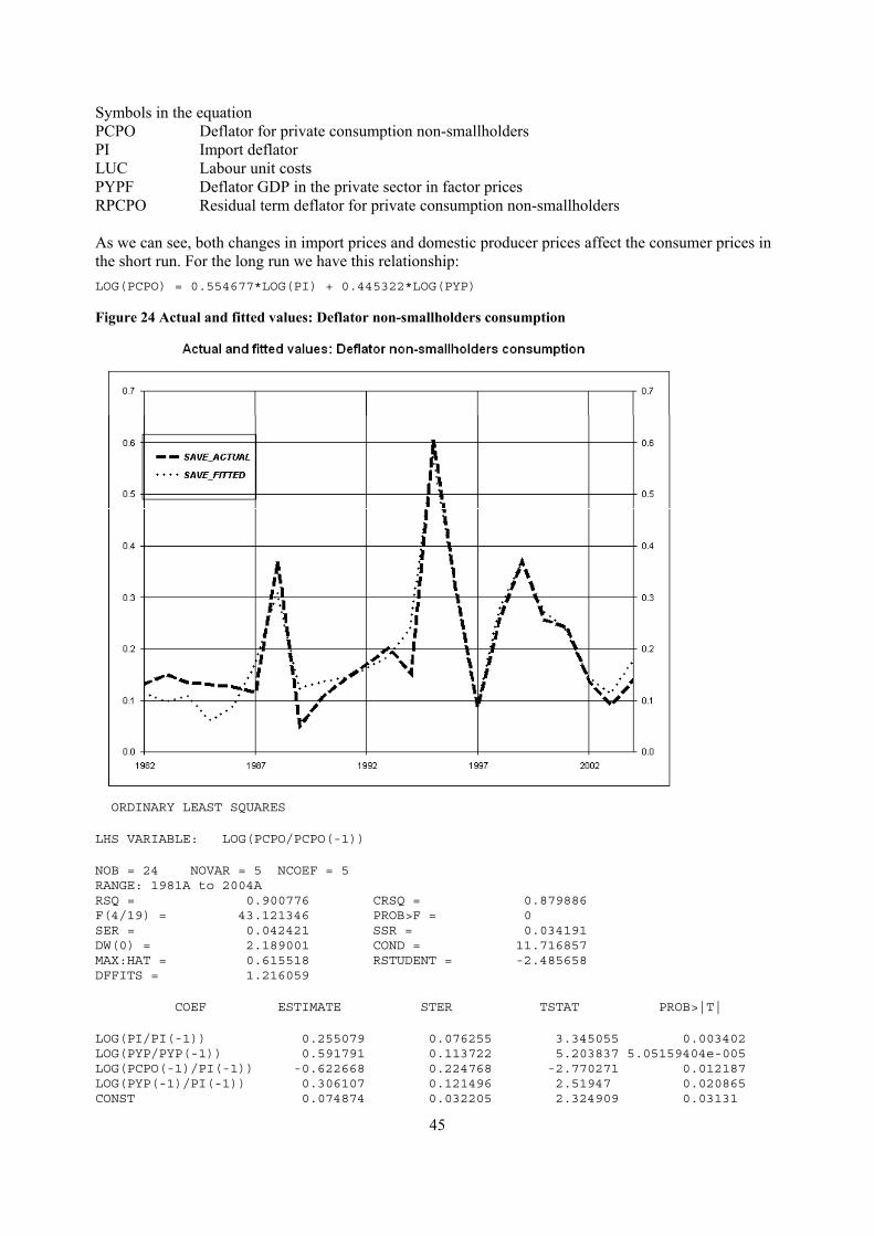
45

Symbols in the equation PCPO Deflator for private consumption non-smallholders PI Import deflator LUC Labour unit costs PYPF Deflator GDP in the private sector in factor prices RPCPO Residual term deflator for private consumption non-smallholders As we can see, both changes in import prices and domestic producer prices affect the consumer prices in the short run. For the long run we have this relationship: LOG(PCPO) = 0.554677*LOG(PI) + 0.445322*LOG(PYP)

Figure 24 Actual and fitted values: Deflator non-smallholders consumption

ORDINARY LEAST SQUARES LHS VARIABLE: LOG(PCPO/PCPO(-1)) NOB = 24 NOVAR = 5 NCOEF = 5 RANGE: 1981A to 2004A RSQ = 0.900776 CRSQ = 0.879886 F(4/19) = 43.121346 PROB>F = 0 SER = 0.042421 SSR = 0.034191 DW(0) = 2.189001 COND = 11.716857 MAX:HAT = 0.615518 RSTUDENT = -2.485658 DFFITS = 1.216059 COEF ESTIMATE STER TSTAT PROB>|T| LOG(PI/PI(-1)) 0.255079 0.076255 3.345055 0.003402 LOG(PYP/PYP(-1)) 0.591791 0.113722 5.203837 5.05159404e-005 LOG(PCPO(-1)/PI(-1)) -0.622668 0.224768 -2.770271 0.012187 LOG(PYP(-1)/PI(-1)) 0.306107 0.121496 2.51947 0.020865 CONST 0.074874 0.032205 2.324909 0.03131

46

Appendix 4.8. Price of investments For the investment prices we have the following estimated relationship: LOG(PJP/PJP(-1)) = 0.107607+0.800961*LOG(PI/PI(-1))-0.5563*LOG(PJP(-1)/PI(-1)) -0.191998*DUM9403+RPJP

There was no significant effect from prices on domestically produced goods, which is plausible if most capital goods are imported.

Figure 25 Actual and fitted values: Deflator private investment

ORDINARY LEAST SQUARES LHS VARIABLE: LOG(PJP/PJP(-1)) NOB = 25 NOVAR = 4 NCOEF = 4 RANGE: 1980A to 2004A RSQ = 0.931511 CRSQ = 0.921727 F(3/21) = 95.206104 PROB>F = 0 SER = 0.03937 SSR = 0.03255 DW(0) = 1.464798 COND = 3.461825 MAX:HAT = 0.512993 RSTUDENT = 2.527708 DFFITS = -1.578176 COEF ESTIMATE STER TSTAT PROB>|T| LOG(PI/PI(-1)) 0.800961 0.051951 15.417535 0 LOG(PJP(-1)/PI(-1)) -0.55636 0.099674 -5.581809 1.53740126e-005 DUM9403 -0.191998 0.029873 -6.427132 2.25969887e-006 CONST 0.107607 0.013835 7.777737 0

47

Recent publications in the series Documents

2004/5 S. Glomsrød and L. Lindholt: The petroleum business environment.

2004/6 H.V. Sæbø: Statistical Metadata on the Internet Revised.

2004/7 M.Bråthen: Collecting data on wages for the Labour - pilot

2004/8 A.L. Brathaug and E. Fløttum: Norwegian Experiences on Treatment of Changes in Methodologies and Classifications when Compiling Long Time Series of National Accounts.

2004/9 L. Røgeberg, T. Skoglund and S. Todsen: Report on the Project Quality Adjusted Input Price Indicies for Collective Services in the Norwegian National Accounts. Report from a Project Co-financed by Eurostat.

2004/10 A-K. Mevik: Uncertainty in the Norwegian Business Tendency Survey.

2004/11 A.G. Hustoft, J. Linnerud and H.V. Sæbø: Quality and metadata in Statistics Norway.

2004/12 E. Engelien, R. Klæboe and Margrete Steinnes: Neighbourhood sonoscapes. Context sensitive noise impact mapping .

2004/13 P. V. Hansen: Regional electricity spot price responses in Norway.

2004/14 A.G. Hustoft and J. Linnerud: Development of a variables documentation system in Statistics Norway. International Statistical Conference "Investment in the future", Prague, Czech Republic, 6-7 September 2004.

2004/15 J.L. Hass: Compilation of data on expenditure in Environmental protection by businesses. Report to the European Commission DG for Environment.

2004/16 A. Raknerud, J. Rønningen og T. Skjerpen: Documentation of the capital database. A database with data for tagible fixed assets and economic data at the firm level.

2004/17 B.K. Wold D. Roll-Hansen A. Mathiassen and S. Opdahl: A Sustainable Household Survey Based Poverty Monitoring System. A Poverty Monitoring System Based upon Household Survey Estimation of Total Consumption. A Preliminary Paper Asking for Cooperation

2004/18 T. Karlsen, D. Quang Pham and T. Skjerpen: Seasonal adjustment and smoothing of manufacturing investments series from the quartely Norwegian national accounts

2005/1 V. Skirbekk: The Impact of a Lower School Leaving Age and a Later Retirement on the

Financing of the Norwegian Public Pension System.

2005/2 H. Utne: The Population and Housing Censushandbook 2001.

2005/3 J. L.Hass and R. Straumann: Environmental Protection Expenditure: Methodological work for the Oil and Gas Extraction Industry. Report to Eurostat.

2005/4 L. Hobbelstad Simpson: National Accounts Supply and Use Tables (SUT) in Constant Prices SNA-NT "SUT/CONSTANT"

2005/5 L. Hobbelstad Simpson: National Accounts Supply and Use Tables (SUT) in Current Prices. SNA-NT "SUT/STARTER"

2005/6 S. Todsen: SNA-NT User's Guide for Supply and Use Tables in Current and Constant Prices.

2005/7 E. Ugreninov, T.M. Normann and A. Andersen: Intermediate Quality Report EU-SILC 2003 Statistics Norway.

2005/8 H.V. Sæbø: Metadata strategy in Statistics Norway. Eurostat Metadata Working Group Luxembourg, 6-7 June 2005.

2005/9 J.L. Hass, K.Ø. Sørensen , K. Erlandsen and T. Smith: Norwegian Economic and Environment Accounts (NOREEA). Project Report 2002.

2005/10 A. Benedictow and T. Harding: Modeling Norwegian balances of financial capital.

2005/11 A.L. Mathiassen,J.B Musoke, P.Opio and P. Schøning: Energy and Poverty A feasibility study on statistics on access and use of energy in Uganda.

2005/12 E. Vinju, R. Strauman, Ø. Skullerud, J. Hass and B. K Frøyen: Statistics on pre-treatment of waste. Pilot study - Norway 2004. Report to Eurostat

2005/13 H. Skullerud, Ø. Skullerud and S. Homstvedt: Pilot study: Treatment of Hazardous Waste. Final report to Eurostat.

2005/14 H. Skiri, B. Strand, M. Talka and H. Brunborg: Selected Documents on the modernisation of the Civil Registration System in Albania Vol. II.

2006/2 T. Åvistland: The problem with a risk premium in a non-stochastic CGE model.