Doc-StartDLBI: Deep learning guided Bayesian inference for structure reconstructionof super-resolution fluorescence microscopyYu Li1,†, Fan Xu2,†, Fa Zhang2, Pingyong Xu3, Mingshu Zhang3, Ming Fan4, Lihua Li4, Xin Gao1,∗, Renmin Han1,∗

1King Abdullah University of Science and Technology (KAUST), Computational Bioscience Research Center (CBRC), Computer,Electrical and Mathematical Sciences and Engineering (CEMSE) Division, Thuwal, 23955-6900, Saudi Arabia. 2High PerformanceComputer Research Center, Institute of Computing Technology, Chinese Academy of Sciences, Beijing 100190, China. 3KeyLaboratory of RNA Biology, Institute of Biophysics, Chinese Academy of Sciences, Beijing 100101, China. 4Institute of BiomedicalEngineering and Instrumentation, Hangzhou Dianzi University, Hangzhou, 310018, China.

ABSTRACTMotivation: Super-resolution fluorescence microscopy, with aresolution beyond the diffraction limit of light, has become anindispensable tool to directly visualize biological structures in livingcells at a nanometer-scale resolution. Despite advances in high-density super-resolution fluorescent techniques, existing methods stillhave bottlenecks, including extremely long execution time, artificialthinning and thickening of structures, and lack of ability to capturelatent structures.Results: Here we propose a novel deep learning guided Bayesianinference approach, DLBI, for the time-series analysis of high-densityfluorescent images. Our method combines the strength of deeplearning and statistical inference, where deep learning captures theunderlying distribution of the fluorophores that are consistent with theobserved time-series fluorescent images by exploring local featuresand correlation along time-axis, and statistical inference further refinesthe ultrastructure extracted by deep learning and endues physicalmeaning to the final image. In particular, our method contains threemain components. The first one is a simulator that takes a high-resolution image as the input, and simulates time-series low-resolutionfluorescent images based on experimentally calibrated parameters,which provides supervised training data to the deep learning model.The second one is a multi-scale deep learning module to captureboth spatial information in each input low-resolution image as wellas temporal information among the time-series images. And the thirdone is a Bayesian inference module that takes the image from thedeep learning module as the initial localization of fluorophores andremoves artifacts by statistical inference. Comprehensive experimentalresults on both real and simulated datasets demonstrate that ourmethod provides more accurate and realistic local patch and large-field reconstruction than the state-of-the-art method, the 3B analysis,while our method is more than two orders of magnitude faster.Availability: The main program is available at https://github.com/lykaust15/DLBI.

1 INTRODUCTIONFluorescence microscopy with a resolution beyond the diffraction limit oflight (i.e., super-resolution) has played an important role in biologicalsciences. The application of super-resolution fluorescence microscopetechniques to living-cell imaging promises dynamic information oncomplex biological structures with nanometer-scale resolution.

Recent development of fluorescence microscopy takes advantages ofboth the development of optical theories and computational methods.Living cell stimulated emission depletion (STED) (Hein et al., 2008),reversible saturable optical linear fluorescence transitions (RESOLFT)(A Schwentker et al., 2007), and structured illumination microscopy(SIM) (Gustafsson, 2005) mainly focus on the innovation of instruments,which requires sophisticated, expensive optical setups and specialized

†These authors contributed equally to this work.∗All correspondence should be addressed to Xin Gao(xin.gao@kaust.edu.sa) and Renmin Han (renmin.han@kaust.edu.sa).

expertise for accurate optical alignment. The time-series analysisbased on localization microscopy techniques, such as photoactivatablelocalization microscopy (PALM) (Hess et al., 2006) and stochastic opticalreconstruction microscopy (STORM) (Rust et al., 2006), is mainly basedon the computational methods, which build a super-resolution imagefrom the localized positions of single molecules in a large number ofimages. Though compared with STED, RESOLFT and SIM, PALM andSTORM do not need specialized microscopes, the localization techniquesof PALM and STORM require the fluorescence emission from individualfluorophores to not overlap with each other, leading to long imaging timeand increased damage to live samples (Lippincott-Schwartz and Manley,2009). More recent methods (Holden et al., 2011; Huang et al., 2011;Quan et al., 2011; Zhu et al., 2012) alleviate the long exposure problemby developing multiple-fluorophore fitting techniques to allow relativelydense fluorescent data, but still do not solve the problem completely.

Bayesian-based time-series analysis of high-density fluorescentimages (Cox et al., 2012; Xu et al., 2015, 2017) further pushes thelimit. By using data from overlapping fluorophores as well as informationfrom blinking and bleaching events, it extends the super-resolutionimaging to the large-field imaging of living cells. Despite its potentialto resolve ultrastructures and fast cellular dynamics in living cells,several bottlenecks still remain. The state-of-the-art methods, such asBayesian analysis of the blinking and bleaching (i.e., the 3B analysis)(Cox et al., 2012), are computationally expensive, and may causeartificial thinning and thickening of structures due to local sampling.Significant improvements on runtime and accuracy have been achieved bysingle molecule-guided Bayesian localization microscopy (SIMBA) (Xuet al., 2017) with the introduction of dual-channel fluorescent imagingand single molecule-guided Bayesian inference. However, the enhancedprocess is severely limited by the specialized class of proteins.

Deep learning has accomplished great success in various fields,including super-resolution imaging (Ledig et al., 2016; Kim et al., 2016;Lim et al., 2017). Among different deep learning architectures, thegenerative adversarial network (GAN) (Goodfellow et al., 2014) achievedthe state-of-the-art performance on single image super-resolution (SISR)(Ledig et al., 2016). However, there are two fundamental differencesbetween the SISR and super-resolution fluorescence microscopy. First,the input of SISR is a downsampled (i.e., low-resolution) image ofa static high-resolution image and the expected output is the originalimage, whereas the input of super-resolution fluorescence microscopy isa time-series of low-resolution fluorescent images and the output is thehigh-resolution image containing estimated locations of the fluorophores(i.e., the reconstructed structure). Second, the nature of SISR ensures thatthere are readily a huge amount of existing data to train deep learningmodels, whereas for fluorescence microscopy, there are only limitedtime-series datasets. Furthermore, most of these datasets do not havethe ground-truth high-resolution images, which make supervised deeplearning infeasible.

In this paper, we propose a novel deep learning guided Bayesianinference framework, DLBI, for structure reconstruction of high-resolution fluorescent microcopy. Our framework combines the strengthof stochastic simulation, deep learning and statistical inference. Toour knowledge, this is the first deep learning-based super-resolution

c© The Author 2017. 1

arX

iv:1

805.

0777

7v2

[cs

.CV

] 2

2 M

ay 2

018

2 Li et al.

fluorescent microscopy method. In particular, the stochastic simulationmodule simulates time-series low-resolution images from high-resolutionimages based on experimentally calibrated parameters of fluorophoresand stochastic modeling, which provides supervised training data fordeep learning models. The deep learning module takes the simulatedtime-series low-resolution images as inputs, captures the underlyingdistribution that generates the ground-truth super-resolutions images byexploring local features and correlation along time-axis of the low-resolution images, and outputs a predicted high-resolution image. Toachieve this goal, we develop a generative adversarial network (GAN)in which a generator network and a discriminator network contest witheach other. The generator network tries to learn the distribution of thehigh-resolution images in a multi-scale manner, whereas the discriminatornetwork tries to discriminate the ground-truth images and the imagesproduced by the generator network. In order to capture the deep featuresin the images, we further ease the degradation issue by integrating residualnetworks (He et al., 2016) into our GAN model, where degradationmeans that stacking more network layers does not lead to better accuracy.The high-resolution image produced by the deep learning module isoften very close to the ground-truth image. However, it can still containsome artifacts, and more importantly, lacks the physical meaning. Thus,we develop the Bayesian inference module to take the predicted high-resolution image from deep learning, run Bayesian inference from theinitial locations of fluorophores in the predicted image, and predict a moreaccurate high-resolution image.

Comprehensive experimental results on two simulated and threereal-world datasets demonstrate that DLBI provides more accurate andrealistic local-patch as well as large-field reconstruction than the state-of-the-art method, the 3B analysis (Cox et al., 2012). Meanwhile, ourmethod is more than 100 times faster than the 3B analysis.

2 MATERIALS AND METHODSAs shown in Fig. 1, DLBI contains three modules: (i) stochasticsimulation (Section 2.1), (ii) deep neural networks (Section 2.2), and (iii)Bayesian inference (Section 2.3).

Fig. 1: The overall workflow of DLBI. The three modules are shown in solid boxes: thesimulation module (green), the deep learning module (red), and the Bayesian inferencemodule (blue). The training (orange) and testing (purple) procedures are shown in dashedboxes. For training, time-series low-resolution images simulated from the simulationmodule are used to train the deep learning module in a multi-scale manner, from 2X,4X, to 8X resolution. For testing, given certain time-series low-resolution images, thedeep learning module predicts the 2X to 8X super-resolution images, and the Bayesianinference module takes the predicted 8X image (which contains artifacts) and produces thefinal high-resolution image.

Although deep learning has proved its great superiority in variousfields, it has not been used for fluorescent microscopy image analysis.One of the possible reasons is the lack of supervised training data,which means the number of time-series low-resolution image datasetsis limited and even for the existing datasets, the ground-truth high-resolution images are often unknown. Here, a stochastic simulation basedon the experimentally calibrated parameters is designed to solve thisissue, without the need of collecting a massive amount of real fluorescentimages. This empowers our deep neural networks to effectively learnthe latent structures under the low-resolution, high-noise and stochasticfluorescing conditions. The primitive super-resolution images produced

by deep neural networks still contain artifacts and lack physical meaning,we finally develop a Bayesian inference module based on the mechanismof fluorophore switching to produce high-confident images.

Our method combines the strength of deep learning and statisticalinference, where deep learning captures the underlying distribution thatgenerates the training super-resolution images by exploring local featuresand correlation along time-axis, and statistical inference removes artifactsand refines the ultrastructure extracted by deep learning, and furtherendues physical meaning to the final image.

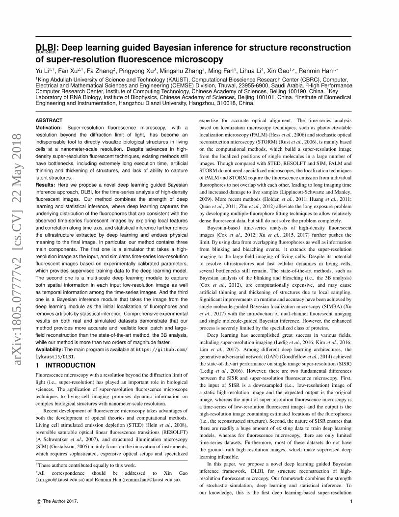
2.1 The stochastic simulation moduleThe input of our simulation module is a high-resolution image that depictsthe distribution of the fluorophores and the output is a time-series of low-resolution fluorescent images with different fluorescing states. We referthe readers to Section S1 for terminologies in fluorescence microscopy.

In our simulation, Laplace-filtered natural images and sketchesare used as the ground-truth high-resolution images that contain thefluorophore distribution. If a gray-scale image is given, the depictedshapes are considered as the distribution of fluorophores and each pixelvalue on the image is considered as the density of fluorophores at thelocation. We then create a number of simulated fluorophores that aredistributed according to the distribution and the densities. For eachfluorophore, it switches according to a Markov model, i.e., amongstates of emitting (activated), not emitting (inactivated), and bleached.The emitting state means that the fluorophore emits photons and aspot according to the point spread function (PSF) is depicted on thecanvas. All the spots of the emitting fluorophores thus result in a high-resolution fluorescent image. Applying the Markov model on the initialhigh-resolution image generates a time-series of high-resolution images.After adding the background to the high-resolution images, they aredownsampled to low-resolution images and noise is finally added. Fig.2 summarizes the stochastic simulation procedure.

Here, the success of simulation relies on three factors: (i) the principalof the linear optical system, (ii) experimentally calibrated parameters offluorophores, and (iii) stochastic modeling.

2.1.1 Linear optics A fluorescence microscope is considered as alinear optical system, in which the superposition principle is valid, i.e.,Image(Obj1 + Obj2) = Image(Obj1) + Image(Obj2). The behavior offluorophores is considered invariant to mutual interaction. Therefore,for high-density fluorescent images, the pixel density can be directlycalculated from the light emitted from its surrounding fluorophores.

When a fluorophore is activated, an observable spot can be recordedby the sensor, the shape of which is called the point spread function (PSF).Considering the limitation of sensor capability, the PSF of an isotropicpoint source is often approximated as a Gaussian function:

I(x, y) = I0 exp(−1

2σ2 ((x − x0)2 + (y − y0)2)), (1)

where σ is calculated from the fluorophore in the specimen that specifiesthe width of the PSF, I0 is the peak intensity and is proportional to the

Fig. 2: The workflow of stochastic simulation. Firstly, a high-resolution image is inputtedas the distribution and density of fluorophores. Then, the emitting of photons is simulatedbased on the stochastic parameters for each time frame. A random background (DC offset)is added to each image. The images are then downsampled to low-resolution and noise isadded, which results in a time-series of low-resolution images.

Deep learning guided Bayesian inference for super-resolution fluorescence microscopy 3

photon emission rate and the single-frame acquisition time, (x0, y0) is thelocation of the fluorophore.

While PSF describes the shape, the full width at half maximum(FWHM) describes the distinguishability. It is defined to be the half widthof the maximum amplitude of PSF. If PSF is modeled as a Gaussianfunction, the relationship between FWHM and σ is given by

FWHM = 2√

2 ln 2 σ ≈ 2.355 σ. (2)

Considering the probability of linear optics, a high-density fluorescentimage is composed by PSFs of the fluorophores.

2.1.2 Calibrated parameters of fluorophores In most imaging systems,the characteristics of a fluorescent protein can be calibrated byexperimental techniques. With all the calibrated parameters, it is notdifficult to describe and simulate the fluorescent switching of a specializedprotein.

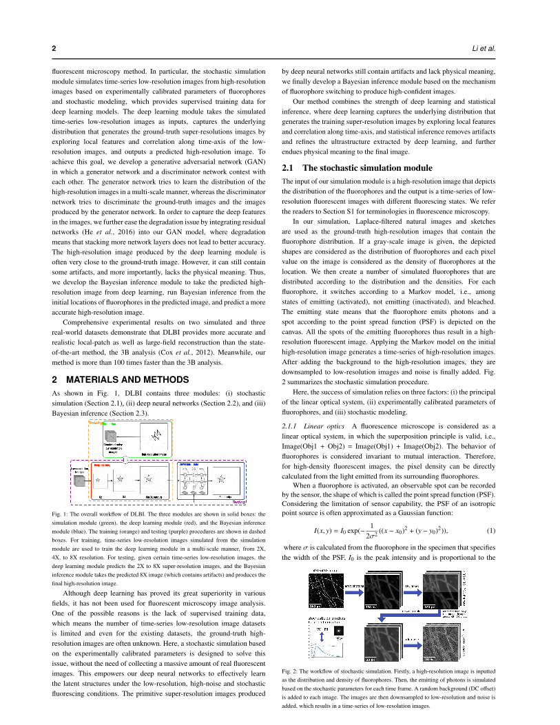
The first characteristic of a fluorophore is its switching probability. Afluorophore always transfers among three states, emitting, not emittingand bleached, which can be specified by a Markov model (Fig. 3). Ifthe fluorophore transfers from not emitting to bleached, it will not emitany photon anymore. As linear optics, each fluorophore’s transitions areassumed to be independent.

Fig. 3: The Markov model describing state transition of a fluorophore.The second characteristic of a fluorophore is its PSF. When a real-

world fluorophore is activated, the emitted photons and its correspondingPSF will not stay unchanged over time. The stochasticity of the PSFand photon strength describes the characteristics of a fluorescent protein.To simulate the fluorescence, we should not ignore these properties.Fortunately, the related parameters can be well-calibrated. The PSF andFWHM of a fluorescent protein can be measured in low molecule density.In an instrument for PALM or STORM, the PSF of the microscope canbe measured by acquiring image frames, fitting the fluorescent spotsparameter, normalizing and then averaging the aligned single-moleculeimages. The distribution of FWHM can be obtained from statisticalanalysis. The principle of linear optics ensures that the parametersmeasured in single-molecule conditions is also applicable to high-densityconditions.

In our simulation, a log-normal distribution (Cox et al., 2012; Zhuet al., 2012) is used to approximate the experimentally measured singlefluorophore photon number distribution. Firstly, a table of fluorophore’sexperimentally calibrated FWHM parameters is used to initialize thePSF table in our simulation, according to Eq.1 and Eq.2. Then for eachfluorophore recorded in the high-resolution image, the state of the currentimage frame is calculated according to the transfer table [P1, P2, P3, P4,P5] (Fig. 3) and a random PSF shape is produced if the correspondingfluorophore is at the “emitting” state. This procedure is repeated for eachfluorophore, which results in the final fluorescent image.

2.1.3 Stochastic modeling The illumination of real-world objects isdifferent at different time. In general, the illumination change of real-world objects can be suppressed by high-pass filtering with a largeGaussian kernel. However, this operation will sharpen the randomnoise and cannot remove the background (or DC offset1). To makeour simulation more realistic, several stochastic factors are introduced.First, for a series of simulated fluorescent images, a background valuecalculated from the multiplication between a random strength factor

1 DC offset, DC bias or DC component denotes the mean value of asignal. If the mean amplitude is zero, there is no DC offset. For mostmicroscopy, the DC offset can be calibrated but cannot be completelyremoved.

and the average image intensity is added to the fluorescent images tosimulate the DC offset. For the same time-series, the strength factorremains unchanged but the background strength changes with the imageintensity. Second, the high-resolution fluorescent image is downsampledand random Gaussian noise is added to the low-resolution image. Here,the noise is also stochastic for different time-series and close to the noisestrength that is measured from the real-world microscopy.

The default setting of our simulation takes a 480 × 480 pixel high-resolution image as the input and simulates 200 frames of 60 × 60 pixel(i.e., 8× binned) low-resolution images.

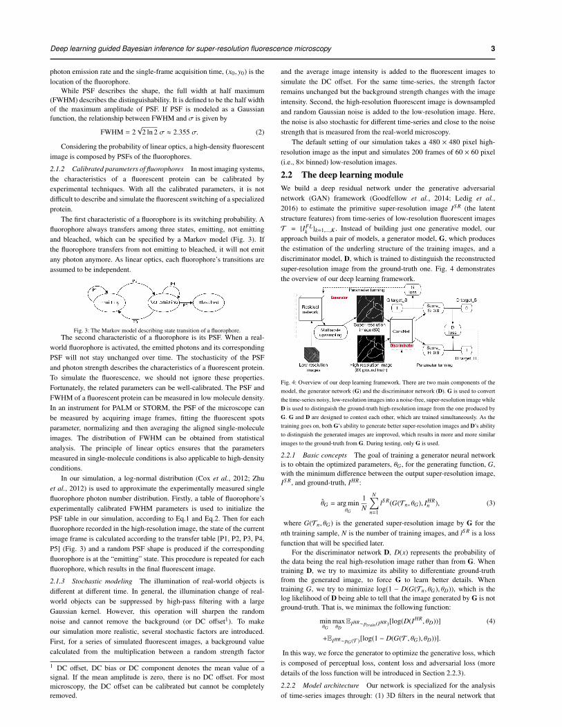
2.2 The deep learning moduleWe build a deep residual network under the generative adversarialnetwork (GAN) framework (Goodfellow et al., 2014; Ledig et al.,2016) to estimate the primitive super-resolution image IS R (the latentstructure features) from time-series of low-resolution fluorescent imagesT = {IFL

k }k=1,...,K . Instead of building just one generative model, ourapproach builds a pair of models, a generator model, G, which producesthe estimation of the underling structure of the training images, and adiscriminator model, D, which is trained to distinguish the reconstructedsuper-resolution image from the ground-truth one. Fig. 4 demonstratesthe overview of our deep learning framework.

Fig. 4: Overview of our deep learning framework. There are two main components of themodel, the generator network (G) and the discriminator network (D). G is used to convertthe time-series noisy, low-resolution images into a noise-free, super-resolution image whileD is used to distinguish the ground-truth high-resolution image from the one produced byG. G and D are designed to contest each other, which are trained simultaneously. As thetraining goes on, both G’s ability to generate better super-resolution images and D’s abilityto distinguish the generated images are improved, which results in more and more similarimages to the ground-truth from G. During testing, only G is used.

2.2.1 Basic concepts The goal of training a generator neural networkis to obtain the optimized parameters, θG , for the generating function, G,with the minimum difference between the output super-resolution image,IS R, and ground-truth, IHR:

θG = arg minθG

1N

N∑n=1

lS R(G(Tn, θG), IHRn ), (3)

where G(Tn, θG) is the generated super-resolution image by G for thenth training sample, N is the number of training images, and lS R is a lossfunction that will be specified later.

For the discriminator network D, D(x) represents the probability ofthe data being the real high-resolution image rather than from G. Whentraining D, we try to maximize its ability to differentiate ground-truthfrom the generated image, to force G to learn better details. Whentraining G, we try to minimize log(1 − D(G(Tn, θG), θD)), which is thelog likelihood of D being able to tell that the image generated by G is notground-truth. That is, we minimax the following function:

minθG

maxθDEIHR∼ptrain(IHR)[log(D(IHR, θD))] (4)

+EIHR∼pG (T )[log(1 − D(G(T , θG), θD))].

In this way, we force the generator to optimize the generative loss, whichis composed of perceptual loss, content loss and adversarial loss (moredetails of the loss function will be introduced in Section 2.2.3).

2.2.2 Model architecture Our network is specialized for the analysisof time-series images through: (1) 3D filters in the neural network that

4 Li et al.

take all the image frames into consideration, which extracts the timedependent information naturally, (2) two specifically designed modulesin the generator residual network, i.e., Monte Carlo dropout (Gal andGhahramani, 2015) and denoise shortcut, to cope with the stochasticswitching of fluorophores and random noise, and (3) a novel incrementalmulti-scale architecture and parameter tuning scheme, which is designedto suppress the error accumulation in large upscaling factor neuralnetworks.

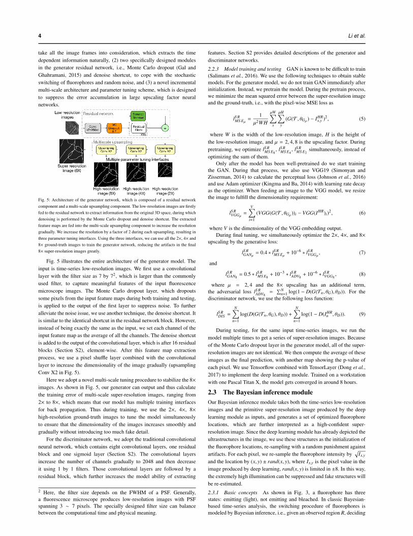
Fig. 5: Architecture of the generator network, which is composed of a residual networkcomponent and a multi-scale upsampling component. The low-resolution images are firstlyfed to the residual network to extract information from the original 3D space, during whichdenoising is performed by the Monte Carlo dropout and denoise shortcut. The extractedfeature maps are fed into the multi-scale upsampling component to increase the resolutiongradually. We increase the resolution by a factor of 2 during each upsampling, resulting inthree parameter tuning interfaces. Using the three interfaces, we can use all the 2×, 4× and8× ground-truth images to train the generator network, reducing the artifacts in the final8× super-resolution images greatly.

Fig. 5 illustrates the entire architecture of the generator model. Theinput is time-series low-resolution images. We first use a convolutionallayer with the filter size as 7 by 72, which is larger than the commonlyused filter, to capture meaningful features of the input fluorescencemicroscope images. The Monte Carlo dropout layer, which dropoutssome pixels from the input feature maps during both training and testing,is applied to the output of the first layer to suppress noise. To furtheralleviate the noise issue, we use another technique, the denoise shortcut. Itis similar to the identical shortcut in the residual network block. However,instead of being exactly the same as the input, we set each channel of theinput feature map as the average of all the channels. The denoise shortcutis added to the output of the convolutional layer, which is after 16 residualblocks (Section S2), element-wise. After this feature map extractionprocess, we use a pixel shuffle layer combined with the convolutionallayer to increase the dimensionality of the image gradually (upsamplingConv X2 in Fig. 5).

Here we adopt a novel multi-scale tuning procedure to stabilize the 8×images. As shown in Fig. 5, our generator can output and thus calculatethe training error of multi-scale super-resolution images, ranging from2× to 8×, which means that our model has multiple training interfacesfor back propagation. Thus during training, we use the 2×, 4×, 8×high-resolution ground-truth images to tune the model simultaneouslyto ensure that the dimensionality of the images increases smoothly andgradually without introducing too much fake detail.

For the discriminator network, we adopt the traditional convolutionalneural network, which contains eight convolutional layers, one residualblock and one sigmoid layer (Section S2). The convolutional layersincrease the number of channels gradually to 2048 and then decreaseit using 1 by 1 filters. Those convolutional layers are followed by aresidual block, which further increases the model ability of extracting

2 Here, the filter size depends on the FWHM of a PSF. Generally,a fluorescence microscope produces low-resolution images with PSFspanning 3 ∼ 7 pixels. The specially designed filter size can balancebetween the computational time and physical meaning.

features. Section S2 provides detailed descriptions of the generator anddiscriminator networks.

2.2.3 Model training and testing GAN is known to be difficult to train(Salimans et al., 2016). We use the following techniques to obtain stablemodels. For the generator model, we do not train GAN immediately afterinitialization. Instead, we pretrain the model. During the pretrain process,we minimize the mean squared error between the super-resolution imageand the ground-truth, i.e., with the pixel-wise MSE loss as

lS RMS Eµ =

1µ2WH

µW∑x

µH∑y

(G(T , θGµ ) − IHRx,y )2, (5)

where W is the width of the low-resolution image, H is the height ofthe low-resolution image, and µ = 2, 4, 8 is the upscaling factor. Duringpretraining, we optimize lS R

MS E8, lS R

MS E4, lS R

MS E2simultaneously, instead of

optimizing the sum of them.Only after the model has been well-pretrained do we start training

the GAN. During that process, we also use VGG19 (Simonyan andZisserman, 2014) to calculate the perceptual loss (Johnson et al., 2016)and use Adam optimizer (Kingma and Ba, 2014) with learning rate decayas the optimizer. When feeding an image to the VGG model, we resizethe image to fulfill the dimensionality requirement:

lS RVGGµ

=

V∑i=1

(VGG(G(T , θGµ ))i − VGG(IHR)i)2, (6)

where V is the dimensionality of the VGG embedding output.During final tuning, we simultaneously optimize the 2×, 4×, and 8×

upscaling by the generative loss:

lS RGANµ = 0.4 ∗ lS R

MS Eµ + 10−6 ∗ lS RVGGµ

, (7)

and

lS RGAN8

= 0.5 ∗ lS RMS E8

+ 10−3 ∗ lS RADV8

+ 10−6 ∗ lS RVGG8

, (8)

where µ = 2, 4 and the 8× upscaling has an additional term,the adversarial loss lS R

ADV8=

∑Nn=1 log(1 − D(G(Tn, θG), θD)). For the

discriminator network, we use the following loss function:

lS RDIS =

N∑n=1

log(D(G(Tn, θG), θD)) +

N∑n=1

log(1 − D(IHRn , θD)). (9)

During testing, for the same input time-series images, we run themodel multiple times to get a series of super-resolution images. Becauseof the Monte Carlo dropout layer in the generator model, all of the super-resolution images are not identical. We then compute the average of theseimages as the final prediction, with another map showing the p-value ofeach pixel. We use Tensorflow combined with TensorLayer (Dong et al.,2017) to implement the deep learning module. Trained on a workstationwith one Pascal Titan X, the model gets converged in around 8 hours.

2.3 The Bayesian inference moduleOur Bayesian inference module takes both the time-series low-resolutionimages and the primitive super-resolution image produced by the deeplearning module as inputs, and generates a set of optimized fluorophorelocations, which are further interpreted as a high-confident super-resolution image. Since the deep learning module has already depicted theultrastructures in the image, we use these structures as the initialization ofthe fluorophore locations, re-sampling with a random punishment againstartifacts. For each pixel, we re-sample the fluorophore intensity by

√Ix,y

and the location by (x, y) ± rand(x, y), where Ix,y is the pixel value in theimage produced by deep learning, rand(x, y) is limited in ±8. In this way,the extremely high illumination can be suppressed and fake structures willbe re-estimated.

2.3.1 Basic concepts As shown in Fig. 3, a fluorophore has threestates: emitting (light), not emitting and bleached. In classic Bayesian-based time-series analysis, the switching procedure of fluorophores ismodeled by Bayesian inference, i.e., given an observed region R, deciding

Deep learning guided Bayesian inference for super-resolution fluorescence microscopy 5

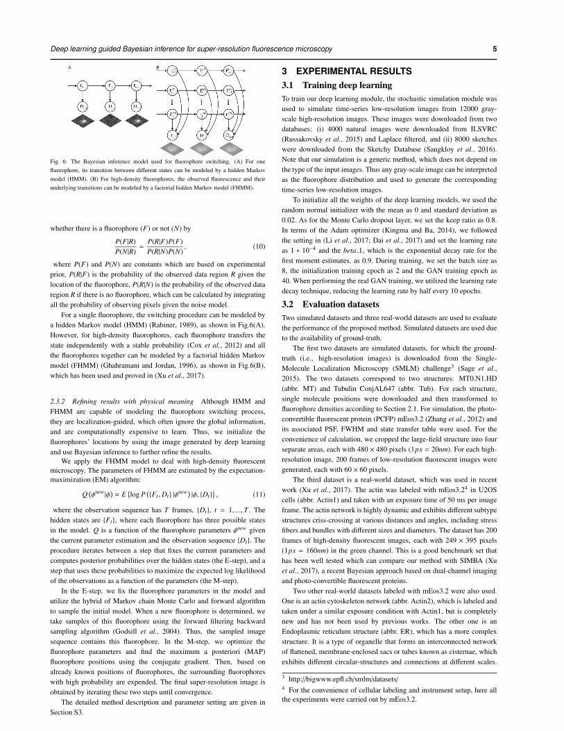
Fig. 6: The Bayesian inference model used for fluorophore switching. (A) For onefluorophore, its transition between different states can be modeled by a hidden Markovmodel (HMM). (B) For high-density fluorophores, the observed fluorescence and theirunderlying transitions can be modeled by a factorial hidden Markov model (FHMM).

whether there is a fluorophore (F) or not (N) by

P(F|R)P(N |R)

=P(R|F)P(F)P(R|N)P(N)

, (10)

where P(F) and P(N) are constants which are based on experimentalprior, P(R|F) is the probability of the observed data region R given thelocation of the fluorophore, P(R|N) is the probability of the observed dataregion R if there is no fluorophore, which can be calculated by integratingall the probability of observing pixels given the noise model.

For a single fluorophore, the switching procedure can be modeled bya hidden Markov model (HMM) (Rabiner, 1989), as shown in Fig.6(A).However, for high-density fluorophores, each fluorophore transfers thestate independently with a stable probability (Cox et al., 2012) and allthe fluorophores together can be modeled by a factorial hidden Markovmodel (FHMM) (Ghahramani and Jordan, 1996), as shown in Fig.6(B),which has been used and proved in (Xu et al., 2017).

2.3.2 Refining results with physical meaning Although HMM andFHMM are capable of modeling the fluorophore switching process,they are localization-guided, which often ignore the global information,and are computationally expensive to learn. Thus, we initialize thefluorophores’ locations by using the image generated by deep learningand use Bayesian inference to further refine the results.

We apply the FHMM model to deal with high-density fluorescentmicroscopy. The parameters of FHMM are estimated by the expectation-maximization (EM) algorithm:

Q(φnew |φ

)= E

{log P

({Ft ,Dt} |φ

new)|φ, {Dt}

}, (11)

where the observation sequence has T frames, {Dt}, t = 1, ...,T . Thehidden states are {Ft}, where each fluorophore has three possible statesin the model. Q is a function of the fluorophore parameters φnew giventhe current parameter estimation and the observation sequence {Dt}. Theprocedure iterates between a step that fixes the current parameters andcomputes posterior probabilities over the hidden states (the E-step), and astep that uses these probabilities to maximize the expected log likelihoodof the observations as a function of the parameters (the M-step).

In the E-step, we fix the fluorophore parameters in the model andutilize the hybrid of Markov chain Monte Carlo and forward algorithmto sample the initial model. When a new fluorophore is determined, wetake samples of this fluorophore using the forward filtering backwardsampling algorithm (Godsill et al., 2004). Thus, the sampled imagesequence contains this fluorophore. In the M-step, we optimize thefluorophore parameters and find the maximum a posteriori (MAP)fluorophore positions using the conjugate gradient. Then, based onalready known positions of fluorophores, the surrounding fluorophoreswith high probability are expended. The final super-resolution image isobtained by iterating these two steps until convergence.

The detailed method description and parameter setting are given inSection S3.

3 EXPERIMENTAL RESULTS3.1 Training deep learningTo train our deep learning module, the stochastic simulation module wasused to simulate time-series low-resolution images from 12000 gray-scale high-resolution images. These images were downloaded from twodatabases: (i) 4000 natural images were downloaded from ILSVRC(Russakovsky et al., 2015) and Laplace filtered, and (ii) 8000 sketcheswere downloaded from the Sketchy Database (Sangkloy et al., 2016).Note that our simulation is a generic method, which does not depend onthe type of the input images. Thus any gray-scale image can be interpretedas the fluorophore distribution and used to generate the correspondingtime-series low-resolution images.

To initialize all the weights of the deep learning models, we used therandom normal initializer with the mean as 0 and standard deviation as0.02. As for the Monte Carlo dropout layer, we set the keep ratio as 0.8.In terms of the Adam optimizer (Kingma and Ba, 2014), we followedthe setting in (Li et al., 2017; Dai et al., 2017) and set the learning rateas 1 ∗ 10−4 and the beta 1, which is the exponential decay rate for thefirst moment estimates, as 0.9. During training, we set the batch size as8, the initialization training epoch as 2 and the GAN training epoch as40. When performing the real GAN training, we utilized the learning ratedecay technique, reducing the learning rate by half every 10 epochs.

3.2 Evaluation datasetsTwo simulated datasets and three real-world datasets are used to evaluatethe performance of the proposed method. Simulated datasets are used dueto the availability of ground-truth.

The first two datasets are simulated datasets, for which the ground-truth (i.e., high-resolution images) is downloaded from the Single-Molecule Localization Microscopy (SMLM) challenge3 (Sage et al.,2015). The two datasets correspond to two structures: MT0.N1.HD(abbr. MT) and Tubulin ConjAL647 (abbr. Tub). For each structure,single molecule positions were downloaded and then transformed tofluorophore densities according to Section 2.1. For simulation, the photo-convertible fluorescent protein (PCFP) mEos3.2 (Zhang et al., 2012) andits associated PSF, FWHM and state transfer table were used. For theconvenience of calculation, we cropped the large-field structure into fourseparate areas, each with 480 × 480 pixels (1px = 20nm). For each high-resolution image, 200 frames of low-resolution fluorescent images weregenerated, each with 60 × 60 pixels.

The third dataset is a real-world dataset, which was used in recentwork (Xu et al., 2017). The actin was labeled with mEos3.24 in U2OScells (abbr. Actin1) and taken with an exposure time of 50 ms per imageframe. The actin network is highly dynamic and exhibits different subtypestructures criss-crossing at various distances and angles, including stressfibers and bundles with different sizes and diameters. The dataset has 200frames of high-density fluorescent images, each with 249 × 395 pixels(1px = 160nm) in the green channel. This is a good benchmark set thathas been well tested which can compare our method with SIMBA (Xuet al., 2017), a recent Bayesian approach based on dual-channel imagingand photo-convertible fluorescent proteins.

Two other real-world datasets labeled with mEos3.2 were also used.One is an actin cytoskeleton network (abbr. Actin2), which is labeled andtaken under a similar exposure condition with Actin1, but is completelynew and has not been used by previous works. The other one is anEndoplasmic reticulum structure (abbr. ER), which has a more complexstructure. It is a type of organelle that forms an interconnected networkof flattened, membrane-enclosed sacs or tubes known as cisternae, whichexhibits different circular-structures and connections at different scales.

3 http://bigwww.epfl.ch/smlm/datasets/4 For the convenience of cellular labeling and instrument setup, here allthe experiments were carried out by mEos3.2.

6 Li et al.

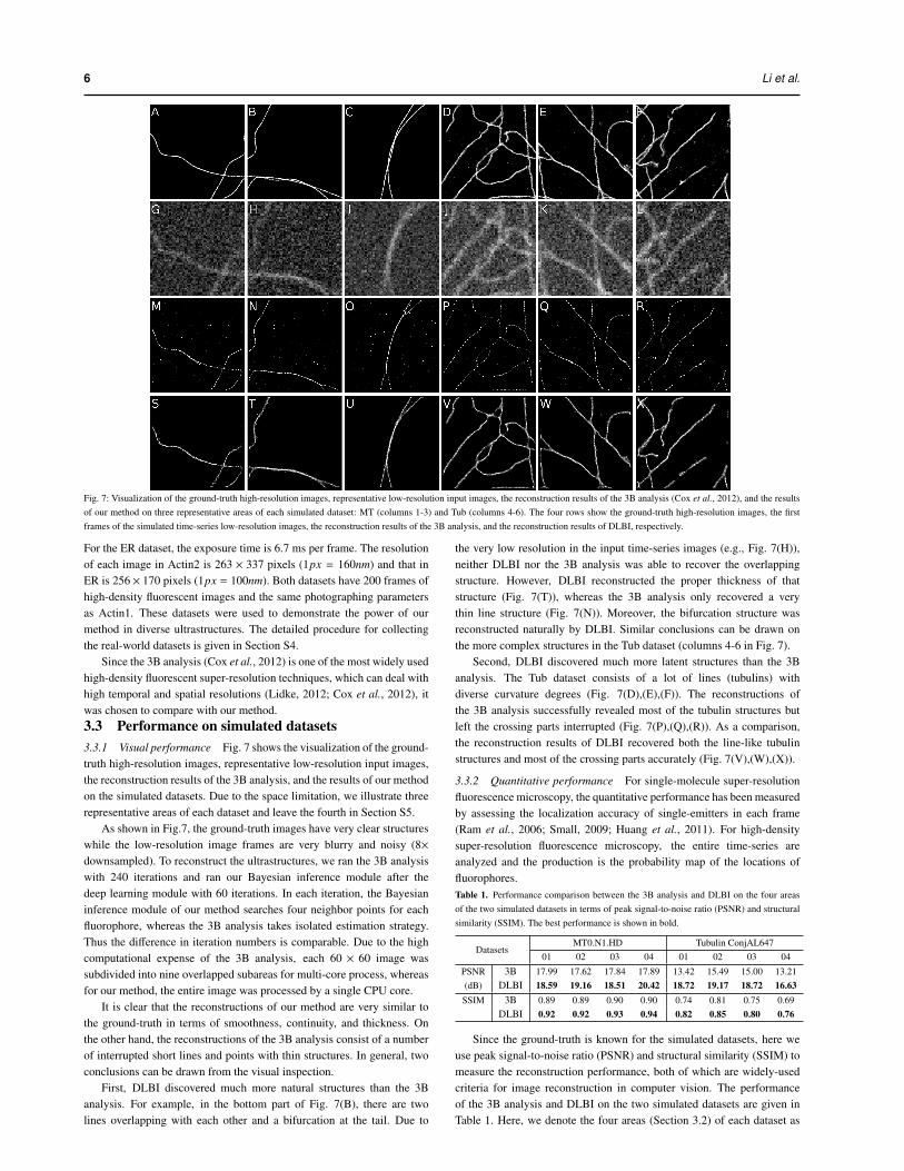
Fig. 7: Visualization of the ground-truth high-resolution images, representative low-resolution input images, the reconstruction results of the 3B analysis (Cox et al., 2012), and the resultsof our method on three representative areas of each simulated dataset: MT (columns 1-3) and Tub (columns 4-6). The four rows show the ground-truth high-resolution images, the firstframes of the simulated time-series low-resolution images, the reconstruction results of the 3B analysis, and the reconstruction results of DLBI, respectively.

For the ER dataset, the exposure time is 6.7 ms per frame. The resolutionof each image in Actin2 is 263 × 337 pixels (1px = 160nm) and that inER is 256 × 170 pixels (1px = 100nm). Both datasets have 200 frames ofhigh-density fluorescent images and the same photographing parametersas Actin1. These datasets were used to demonstrate the power of ourmethod in diverse ultrastructures. The detailed procedure for collectingthe real-world datasets is given in Section S4.

Since the 3B analysis (Cox et al., 2012) is one of the most widely usedhigh-density fluorescent super-resolution techniques, which can deal withhigh temporal and spatial resolutions (Lidke, 2012; Cox et al., 2012), itwas chosen to compare with our method.3.3 Performance on simulated datasets3.3.1 Visual performance Fig. 7 shows the visualization of the ground-truth high-resolution images, representative low-resolution input images,the reconstruction results of the 3B analysis, and the results of our methodon the simulated datasets. Due to the space limitation, we illustrate threerepresentative areas of each dataset and leave the fourth in Section S5.

As shown in Fig.7, the ground-truth images have very clear structureswhile the low-resolution image frames are very blurry and noisy (8×downsampled). To reconstruct the ultrastructures, we ran the 3B analysiswith 240 iterations and ran our Bayesian inference module after thedeep learning module with 60 iterations. In each iteration, the Bayesianinference module of our method searches four neighbor points for eachfluorophore, whereas the 3B analysis takes isolated estimation strategy.Thus the difference in iteration numbers is comparable. Due to the highcomputational expense of the 3B analysis, each 60 × 60 image wassubdivided into nine overlapped subareas for multi-core process, whereasfor our method, the entire image was processed by a single CPU core.

It is clear that the reconstructions of our method are very similar tothe ground-truth in terms of smoothness, continuity, and thickness. Onthe other hand, the reconstructions of the 3B analysis consist of a numberof interrupted short lines and points with thin structures. In general, twoconclusions can be drawn from the visual inspection.

First, DLBI discovered much more natural structures than the 3Banalysis. For example, in the bottom part of Fig. 7(B), there are twolines overlapping with each other and a bifurcation at the tail. Due to

the very low resolution in the input time-series images (e.g., Fig. 7(H)),neither DLBI nor the 3B analysis was able to recover the overlappingstructure. However, DLBI reconstructed the proper thickness of thatstructure (Fig. 7(T)), whereas the 3B analysis only recovered a verythin line structure (Fig. 7(N)). Moreover, the bifurcation structure wasreconstructed naturally by DLBI. Similar conclusions can be drawn onthe more complex structures in the Tub dataset (columns 4-6 in Fig. 7).

Second, DLBI discovered much more latent structures than the 3Banalysis. The Tub dataset consists of a lot of lines (tubulins) withdiverse curvature degrees (Fig. 7(D),(E),(F)). The reconstructions ofthe 3B analysis successfully revealed most of the tubulin structures butleft the crossing parts interrupted (Fig. 7(P),(Q),(R)). As a comparison,the reconstruction results of DLBI recovered both the line-like tubulinstructures and most of the crossing parts accurately (Fig. 7(V),(W),(X)).

3.3.2 Quantitative performance For single-molecule super-resolutionfluorescence microscopy, the quantitative performance has been measuredby assessing the localization accuracy of single-emitters in each frame(Ram et al., 2006; Small, 2009; Huang et al., 2011). For high-densitysuper-resolution fluorescence microscopy, the entire time-series areanalyzed and the production is the probability map of the locations offluorophores.Table 1. Performance comparison between the 3B analysis and DLBI on the four areasof the two simulated datasets in terms of peak signal-to-noise ratio (PSNR) and structuralsimilarity (SSIM). The best performance is shown in bold.

DatasetsMT0.N1.HD Tubulin ConjAL647

01 02 03 04 01 02 03 04

PSNR 3B 17.99 17.62 17.84 17.89 13.42 15.49 15.00 13.21(dB) DLBI 18.59 19.16 18.51 20.42 18.72 19.17 18.72 16.63

SSIM 3B 0.89 0.89 0.90 0.90 0.74 0.81 0.75 0.69DLBI 0.92 0.92 0.93 0.94 0.82 0.85 0.80 0.76

Since the ground-truth is known for the simulated datasets, here weuse peak signal-to-noise ratio (PSNR) and structural similarity (SSIM) tomeasure the reconstruction performance, both of which are widely-usedcriteria for image reconstruction in computer vision. The performanceof the 3B analysis and DLBI on the two simulated datasets are given inTable 1. Here, we denote the four areas (Section 3.2) of each dataset as

Deep learning guided Bayesian inference for super-resolution fluorescence microscopy 7

“01”, “02”, “03” and “04”, respectively. It can be seen that DLBI clearlyoutperforms the 3B analysis in terms of both PSNR and SSIM on all theareas of the two datasets.

3.4 Performance on real datasetsFig. 8 shows the first frame of the time-series fluorescent images foreach of the three real-world datasets. Here we evaluate the performanceof our method for both local-patch reconstruction (areas selected bygreen rectangles) and large-field reconstruction (areas selected by yellowrectangles).

Fig. 8: The first frame of the time-series fluorescent images for each of the three real-worlddatasets: (A) Actin1 (Xu et al., 2017), (B) Actin2, and (C) ER.

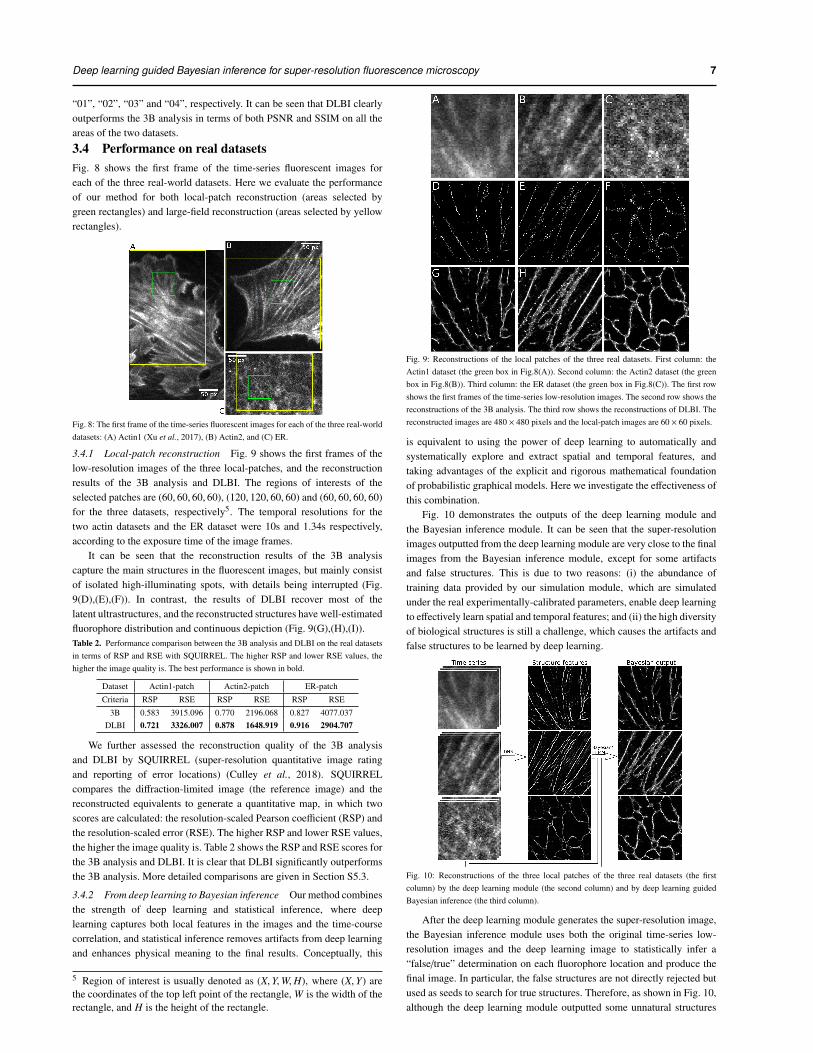
3.4.1 Local-patch reconstruction Fig. 9 shows the first frames of thelow-resolution images of the three local-patches, and the reconstructionresults of the 3B analysis and DLBI. The regions of interests of theselected patches are (60, 60, 60, 60), (120, 120, 60, 60) and (60, 60, 60, 60)for the three datasets, respectively5. The temporal resolutions for thetwo actin datasets and the ER dataset were 10s and 1.34s respectively,according to the exposure time of the image frames.

It can be seen that the reconstruction results of the 3B analysiscapture the main structures in the fluorescent images, but mainly consistof isolated high-illuminating spots, with details being interrupted (Fig.9(D),(E),(F)). In contrast, the results of DLBI recover most of thelatent ultrastructures, and the reconstructed structures have well-estimatedfluorophore distribution and continuous depiction (Fig. 9(G),(H),(I)).Table 2. Performance comparison between the 3B analysis and DLBI on the real datasetsin terms of RSP and RSE with SQUIRREL. The higher RSP and lower RSE values, thehigher the image quality is. The best performance is shown in bold.

Dataset Actin1-patch Actin2-patch ER-patch

Criteria RSP RSE RSP RSE RSP RSE

3B 0.583 3915.096 0.770 2196.068 0.827 4077.037DLBI 0.721 3326.007 0.878 1648.919 0.916 2904.707

We further assessed the reconstruction quality of the 3B analysisand DLBI by SQUIRREL (super-resolution quantitative image ratingand reporting of error locations) (Culley et al., 2018). SQUIRRELcompares the diffraction-limited image (the reference image) and thereconstructed equivalents to generate a quantitative map, in which twoscores are calculated: the resolution-scaled Pearson coefficient (RSP) andthe resolution-scaled error (RSE). The higher RSP and lower RSE values,the higher the image quality is. Table 2 shows the RSP and RSE scores forthe 3B analysis and DLBI. It is clear that DLBI significantly outperformsthe 3B analysis. More detailed comparisons are given in Section S5.3.

3.4.2 From deep learning to Bayesian inference Our method combinesthe strength of deep learning and statistical inference, where deeplearning captures both local features in the images and the time-coursecorrelation, and statistical inference removes artifacts from deep learningand enhances physical meaning to the final results. Conceptually, this

5 Region of interest is usually denoted as (X,Y,W,H), where (X,Y) arethe coordinates of the top left point of the rectangle, W is the width of therectangle, and H is the height of the rectangle.

Fig. 9: Reconstructions of the local patches of the three real datasets. First column: theActin1 dataset (the green box in Fig.8(A)). Second column: the Actin2 dataset (the greenbox in Fig.8(B)). Third column: the ER dataset (the green box in Fig.8(C)). The first rowshows the first frames of the time-series low-resolution images. The second row shows thereconstructions of the 3B analysis. The third row shows the reconstructions of DLBI. Thereconstructed images are 480 × 480 pixels and the local-patch images are 60 × 60 pixels.

is equivalent to using the power of deep learning to automatically andsystematically explore and extract spatial and temporal features, andtaking advantages of the explicit and rigorous mathematical foundationof probabilistic graphical models. Here we investigate the effectiveness ofthis combination.

Fig. 10 demonstrates the outputs of the deep learning module andthe Bayesian inference module. It can be seen that the super-resolutionimages outputted from the deep learning module are very close to the finalimages from the Bayesian inference module, except for some artifactsand false structures. This is due to two reasons: (i) the abundance oftraining data provided by our simulation module, which are simulatedunder the real experimentally-calibrated parameters, enable deep learningto effectively learn spatial and temporal features; and (ii) the high diversityof biological structures is still a challenge, which causes the artifacts andfalse structures to be learned by deep learning.

Fig. 10: Reconstructions of the three local patches of the three real datasets (the firstcolumn) by the deep learning module (the second column) and by deep learning guidedBayesian inference (the third column).

After the deep learning module generates the super-resolution image,the Bayesian inference module uses both the original time-series low-resolution images and the deep learning image to statistically infer a“false/true” determination on each fluorophore location and produce thefinal image. In particular, the false structures are not directly rejected butused as seeds to search for true structures. Therefore, as shown in Fig. 10,although the deep learning module outputted some unnatural structures

8 Li et al.

for the Actin2 and ER datasets, these structures were further corrected bythe Bayesian inference module.

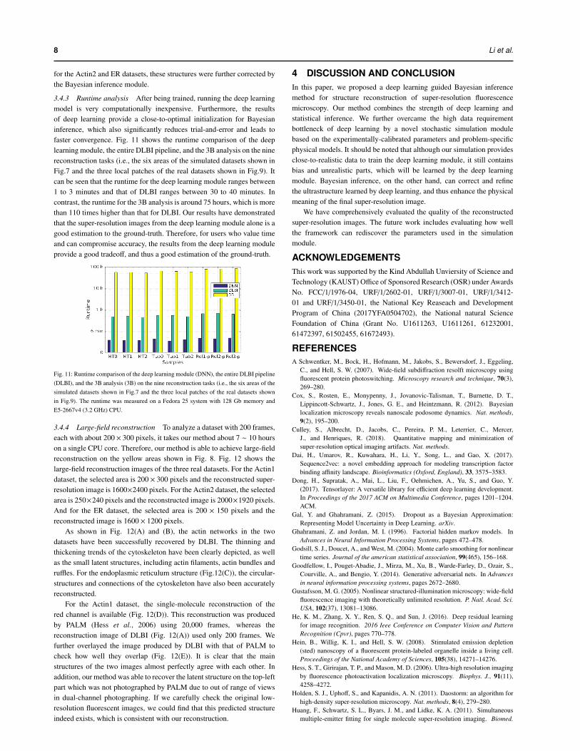
3.4.3 Runtime analysis After being trained, running the deep learningmodel is very computationally inexpensive. Furthermore, the resultsof deep learning provide a close-to-optimal initialization for Bayesianinference, which also significantly reduces trial-and-error and leads tofaster convergence. Fig. 11 shows the runtime comparison of the deeplearning module, the entire DLBI pipeline, and the 3B analysis on the ninereconstruction tasks (i.e., the six areas of the simulated datasets shown inFig.7 and the three local patches of the real datasets shown in Fig.9). Itcan be seen that the runtime for the deep learning module ranges between1 to 3 minutes and that of DLBI ranges between 30 to 40 minutes. Incontrast, the runtime for the 3B analysis is around 75 hours, which is morethan 110 times higher than that for DLBI. Our results have demonstratedthat the super-resolution images from the deep learning module alone is agood estimation to the ground-truth. Therefore, for users who value timeand can compromise accuracy, the results from the deep learning moduleprovide a good tradeoff, and thus a good estimation of the ground-truth.

Fig. 11: Runtime comparison of the deep learning module (DNN), the entire DLBI pipeline(DLBI), and the 3B analysis (3B) on the nine reconstruction tasks (i.e., the six areas of thesimulated datasets shown in Fig.7 and the three local patches of the real datasets shownin Fig.9). The runtime was measured on a Fedora 25 system with 128 Gb memory andE5-2667v4 (3.2 GHz) CPU.

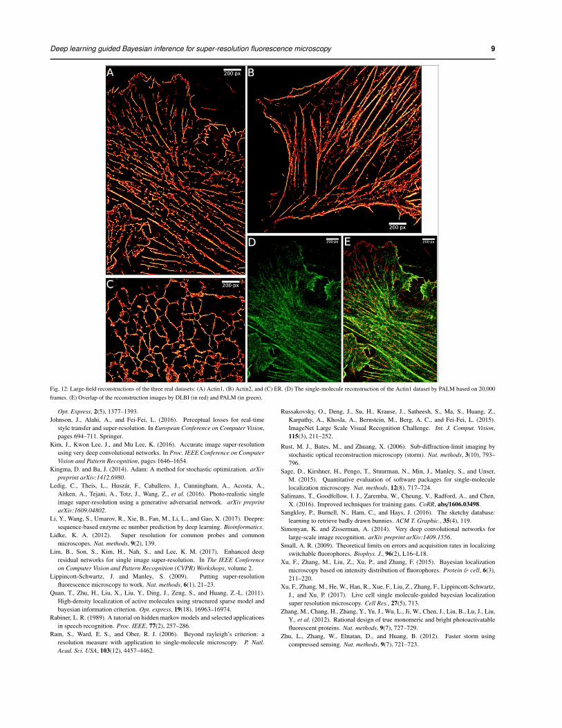
3.4.4 Large-field reconstruction To analyze a dataset with 200 frames,each with about 200 × 300 pixels, it takes our method about 7 ∼ 10 hourson a single CPU core. Therefore, our method is able to achieve large-fieldreconstruction on the yellow areas shown in Fig. 8. Fig. 12 shows thelarge-field reconstruction images of the three real datasets. For the Actin1dataset, the selected area is 200 × 300 pixels and the reconstructed super-resolution image is 1600×2400 pixels. For the Actin2 dataset, the selectedarea is 250×240 pixels and the reconstructed image is 2000×1920 pixels.And for the ER dataset, the selected area is 200 × 150 pixels and thereconstructed image is 1600 × 1200 pixels.

As shown in Fig. 12(A) and (B), the actin networks in the twodatasets have been successfully recovered by DLBI. The thinning andthickening trends of the cytoskeleton have been clearly depicted, as wellas the small latent structures, including actin filaments, actin bundles andruffles. For the endoplasmic reticulum structure (Fig.12(C)), the circular-structures and connections of the cytoskeleton have also been accuratelyreconstructed.

For the Actin1 dataset, the single-molecule reconstruction of thered channel is available (Fig. 12(D)). This reconstruction was producedby PALM (Hess et al., 2006) using 20,000 frames, whereas thereconstruction image of DLBI (Fig. 12(A)) used only 200 frames. Wefurther overlayed the image produced by DLBI with that of PALM tocheck how well they overlap (Fig. 12(E)). It is clear that the mainstructures of the two images almost perfectly agree with each other. Inaddition, our method was able to recover the latent structure on the top-leftpart which was not photographed by PALM due to out of range of viewsin dual-channel photographing. If we carefully check the original low-resolution fluorescent images, we could find that this predicted structureindeed exists, which is consistent with our reconstruction.

4 DISCUSSION AND CONCLUSIONIn this paper, we proposed a deep learning guided Bayesian inferencemethod for structure reconstruction of super-resolution fluorescencemicroscopy. Our method combines the strength of deep learning andstatistical inference. We further overcame the high data requirementbottleneck of deep learning by a novel stochastic simulation modulebased on the experimentally-calibrated parameters and problem-specificphysical models. It should be noted that although our simulation providesclose-to-realistic data to train the deep learning module, it still containsbias and unrealistic parts, which will be learned by the deep learningmodule. Bayesian inference, on the other hand, can correct and refinethe ultrastructure learned by deep learning, and thus enhance the physicalmeaning of the final super-resolution image.

We have comprehensively evaluated the quality of the reconstructedsuper-resolution images. The future work includes evaluating how wellthe framework can rediscover the parameters used in the simulationmodule.

ACKNOWLEDGEMENTSThis work was supported by the Kind Abdullah Unviersity of Science andTechnology (KAUST) Office of Sponsored Research (OSR) under AwardsNo. FCC/1/1976-04, URF/1/2602-01, URF/1/3007-01, URF/1/3412-01 and URF/1/3450-01, the National Key Reaseach and DevelopmentProgram of China (2017YFA0504702), the National natural ScienceFoundation of China (Grant No. U1611263, U1611261, 61232001,61472397, 61502455, 61672493).

REFERENCESA Schwentker, M., Bock, H., Hofmann, M., Jakobs, S., Bewersdorf, J., Eggeling,

C., and Hell, S. W. (2007). Wide-field subdiffraction resolft microscopy usingfluorescent protein photoswitching. Microscopy research and technique, 70(3),269–280.

Cox, S., Rosten, E., Monypenny, J., Jovanovic-Talisman, T., Burnette, D. T.,Lippincott-Schwartz, J., Jones, G. E., and Heintzmann, R. (2012). Bayesianlocalization microscopy reveals nanoscale podosome dynamics. Nat. methods,9(2), 195–200.

Culley, S., Albrecht, D., Jacobs, C., Pereira, P. M., Leterrier, C., Mercer,J., and Henriques, R. (2018). Quantitative mapping and minimization ofsuper-resolution optical imaging artifacts. Nat. methods.

Dai, H., Umarov, R., Kuwahara, H., Li, Y., Song, L., and Gao, X. (2017).Sequence2vec: a novel embedding approach for modeling transcription factorbinding affinity landscape. Bioinformatics (Oxford, England), 33, 3575–3583.

Dong, H., Supratak, A., Mai, L., Liu, F., Oehmichen, A., Yu, S., and Guo, Y.(2017). Tensorlayer: A versatile library for efficient deep learning development.In Proceedings of the 2017 ACM on Multimedia Conference, pages 1201–1204.ACM.

Gal, Y. and Ghahramani, Z. (2015). Dropout as a Bayesian Approximation:Representing Model Uncertainty in Deep Learning. arXiv.

Ghahramani, Z. and Jordan, M. I. (1996). Factorial hidden markov models. InAdvances in Neural Information Processing Systems, pages 472–478.

Godsill, S. J., Doucet, A., and West, M. (2004). Monte carlo smoothing for nonlineartime series. Journal of the american statistical association, 99(465), 156–168.

Goodfellow, I., Pouget-Abadie, J., Mirza, M., Xu, B., Warde-Farley, D., Ozair, S.,Courville, A., and Bengio, Y. (2014). Generative adversarial nets. In Advancesin neural information processing systems, pages 2672–2680.

Gustafsson, M. G. (2005). Nonlinear structured-illumination microscopy: wide-fieldfluorescence imaging with theoretically unlimited resolution. P. Natl. Acad. Sci.USA, 102(37), 13081–13086.

He, K. M., Zhang, X. Y., Ren, S. Q., and Sun, J. (2016). Deep residual learningfor image recognition. 2016 Ieee Conference on Computer Vision and PatternRecognition (Cpvr), pages 770–778.

Hein, B., Willig, K. I., and Hell, S. W. (2008). Stimulated emission depletion(sted) nanoscopy of a fluorescent protein-labeled organelle inside a living cell.Proceedings of the National Academy of Sciences, 105(38), 14271–14276.

Hess, S. T., Girirajan, T. P., and Mason, M. D. (2006). Ultra-high resolution imagingby fluorescence photoactivation localization microscopy. Biophys. J., 91(11),4258–4272.

Holden, S. J., Uphoff, S., and Kapanidis, A. N. (2011). Daostorm: an algorithm forhigh-density super-resolution microscopy. Nat. methods, 8(4), 279–280.

Huang, F., Schwartz, S. L., Byars, J. M., and Lidke, K. A. (2011). Simultaneousmultiple-emitter fitting for single molecule super-resolution imaging. Biomed.

Deep learning guided Bayesian inference for super-resolution fluorescence microscopy 9

Fig. 12: Large-field reconstructions of the three real datasets: (A) Actin1, (B) Actin2, and (C) ER. (D) The single-molecule reconstruction of the Actin1 dataset by PALM based on 20,000frames. (E) Overlap of the reconstruction images by DLBI (in red) and PALM (in green).

Opt. Express, 2(5), 1377–1393.Johnson, J., Alahi, A., and Fei-Fei, L. (2016). Perceptual losses for real-time

style transfer and super-resolution. In European Conference on Computer Vision,pages 694–711. Springer.

Kim, J., Kwon Lee, J., and Mu Lee, K. (2016). Accurate image super-resolutionusing very deep convolutional networks. In Proc. IEEE Conference on ComputerVision and Pattern Recognition, pages 1646–1654.

Kingma, D. and Ba, J. (2014). Adam: A method for stochastic optimization. arXivpreprint arXiv:1412.6980.

Ledig, C., Theis, L., Huszar, F., Caballero, J., Cunningham, A., Acosta, A.,Aitken, A., Tejani, A., Totz, J., Wang, Z., et al. (2016). Photo-realistic singleimage super-resolution using a generative adversarial network. arXiv preprintarXiv:1609.04802.

Li, Y., Wang, S., Umarov, R., Xie, B., Fan, M., Li, L., and Gao, X. (2017). Deepre:sequence-based enzyme ec number prediction by deep learning. Bioinformatics.

Lidke, K. A. (2012). Super resolution for common probes and commonmicroscopes. Nat. methods, 9(2), 139.

Lim, B., Son, S., Kim, H., Nah, S., and Lee, K. M. (2017). Enhanced deepresidual networks for single image super-resolution. In The IEEE Conferenceon Computer Vision and Pattern Recognition (CVPR) Workshops, volume 2.

Lippincott-Schwartz, J. and Manley, S. (2009). Putting super-resolutionfluorescence microscopy to work. Nat. methods, 6(1), 21–23.

Quan, T., Zhu, H., Liu, X., Liu, Y., Ding, J., Zeng, S., and Huang, Z.-L. (2011).High-density localization of active molecules using structured sparse model andbayesian information criterion. Opt. express, 19(18), 16963–16974.

Rabiner, L. R. (1989). A tutorial on hidden markov models and selected applicationsin speech recognition. Proc. IEEE, 77(2), 257–286.

Ram, S., Ward, E. S., and Ober, R. J. (2006). Beyond rayleigh’s criterion: aresolution measure with application to single-molecule microscopy. P. Natl.Acad. Sci. USA, 103(12), 4457–4462.

Russakovsky, O., Deng, J., Su, H., Krause, J., Satheesh, S., Ma, S., Huang, Z.,Karpathy, A., Khosla, A., Bernstein, M., Berg, A. C., and Fei-Fei, L. (2015).ImageNet Large Scale Visual Recognition Challenge. Int. J. Comput. Vision,115(3), 211–252.

Rust, M. J., Bates, M., and Zhuang, X. (2006). Sub-diffraction-limit imaging bystochastic optical reconstruction microscopy (storm). Nat. methods, 3(10), 793–796.

Sage, D., Kirshner, H., Pengo, T., Stuurman, N., Min, J., Manley, S., and Unser,M. (2015). Quantitative evaluation of software packages for single-moleculelocalization microscopy. Nat. methods, 12(8), 717–724.

Salimans, T., Goodfellow, I. J., Zaremba, W., Cheung, V., Radford, A., and Chen,X. (2016). Improved techniques for training gans. CoRR, abs/1606.03498.

Sangkloy, P., Burnell, N., Ham, C., and Hays, J. (2016). The sketchy database:learning to retrieve badly drawn bunnies. ACM T. Graphic., 35(4), 119.

Simonyan, K. and Zisserman, A. (2014). Very deep convolutional networks forlarge-scale image recognition. arXiv preprint arXiv:1409.1556.

Small, A. R. (2009). Theoretical limits on errors and acquisition rates in localizingswitchable fluorophores. Biophys. J., 96(2), L16–L18.

Xu, F., Zhang, M., Liu, Z., Xu, P., and Zhang, F. (2015). Bayesian localizationmicroscopy based on intensity distribution of fluorophores. Protein & cell, 6(3),211–220.

Xu, F., Zhang, M., He, W., Han, R., Xue, F., Liu, Z., Zhang, F., Lippincott-Schwartz,J., and Xu, P. (2017). Live cell single molecule-guided bayesian localizationsuper resolution microscopy. Cell Res., 27(5), 713.

Zhang, M., Chang, H., Zhang, Y., Yu, J., Wu, L., Ji, W., Chen, J., Liu, B., Lu, J., Liu,Y., et al. (2012). Rational design of true monomeric and bright photoactivatablefluorescent proteins. Nat. methods, 9(7), 727–729.

Zhu, L., Zhang, W., Elnatan, D., and Huang, B. (2012). Faster storm usingcompressed sensing. Nat. methods, 9(7), 721–723.