Embed Size (px)
Citation preview
DLA 1
New Jersey Institute of Technology
Monte Carlo Methods of Diffusion Limited Aggregation
Lucas Lamb
Antonio J. Jurko
Julia Porrino
Andrea Roeser
Sarp Uslu
Math 451H Spring 2015
Lou Kondic
May 12, 2015
DLA 2
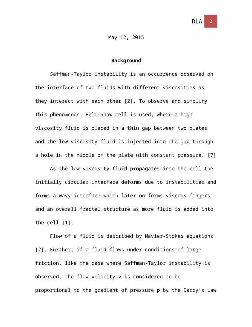
Background
Saffman-Taylor instability is an occurrence observed on the interface of two fluids
with different viscosities as they interact with each other [2]. To observe and simplify this
phenomenon, Hele-Shaw cell is used, where a high viscosity fluid is placed in a thin gap
between two plates and the low viscosity fluid is injected into the gap through a hole in the
middle of the plate with constant pressure. [7]
As the low viscosity fluid propagates into the cell the initially circular interface
deforms due to instabilities and forms a wavy interface which later on forms viscous fingers
and an overall fractal structure as more fluid is added into the cell [1].
Flow of a fluid is described by Navier-Stokes equations [2]. Further, if a fluid flows
under conditions of large friction, like the case where Saffman-Taylor instability is
observed, the flow velocity v is considered to be proportional to the gradient of
pressure p by the Darcy’s Law [2]. Along with the incompressibility assumption (div v =
0), thus the pressure field satisfies Laplace’s equation [6].
DLA simulation is a specific random walk and the limit of the random walk is
Brownian motion which describes diffusion [2]. Similar to the fluid velocity in Darcy’s
Law, the flux of random walkers (growth velocity) is considered to be proportional to the
gradient of probability field ϕ (probability of finding a walker at some point). Since the
walkers are only allowed to stick to the aggregate and not allowed to wander away
(boundary conditions such that ϕ = 0 on aggregate and ϕ = 1 where walkers are launched),
divergence of flux is zero [7]. Again, the Laplace’s equation is obtained.
Results that are obtained from the DLA simulations look like scale invariant
structures. Even though there is no way to prove that the results are fractals, one way to
DLA 3
analyze whether these simulations are accurate is to measure the fractal dimension and
compare it to the fractal dimension obtained from the experiments. This approach makes
sense because fractal dimension is considered to be a universal quantity, which is somewhat
independent of microscopic interactions during the growth of the aggregate.
Description of Method
The walkers begin walking from the outer edge of a circle whose center is the initial
seed. The place the walker starts from is random and the movement the walker follows is
also random— the walker moves north, south, east, or west until it reaches a previously
stuck walker. The only thing a walker cannot do is leave the circle and if they attempt to do
so, a new random movement is generated. As the aggregate of walkers grows larger, the
circle expands to contain the entire aggregate [7].
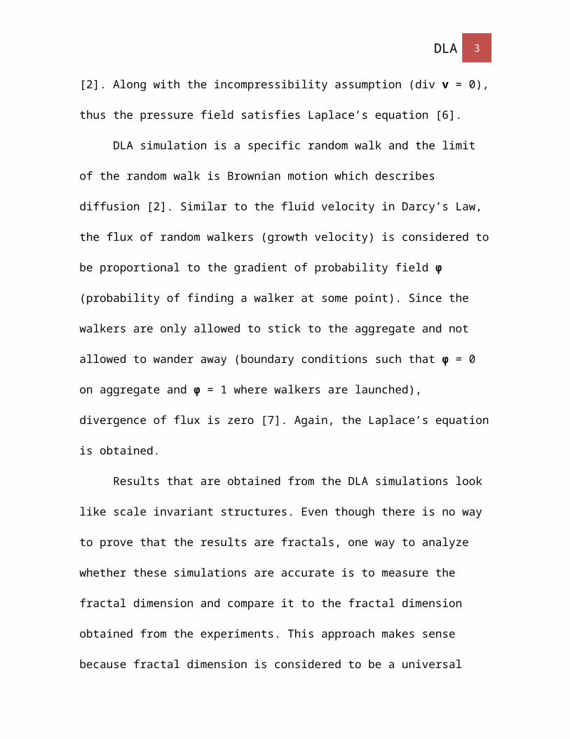
When the walkers arrive next to an already occupied space, the walker makes an
attempt to stick at this location. The probability of the walker sticking is based on the local
curvature, which simulates the surface tension of the fluid in the Hele-Shaw cell. This
probability is calculated in our code by the “findprob” function, which returns the sticking
probability P.
Figure 1: The gold boxes are occupied locations of the
aggregate. The green box is the walker moving randomly
around the space. The pink boxes represent the possible
locations the walker can stick to if the code allows it (by
calculating the sticking probability using the local curvature).
DLA 4
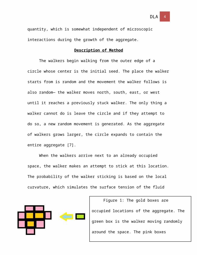
Calculation of the sticking probability follows the method proposed by Vicsek
closely; sticking probability is linearly dependent on the number of occupied spaces around
the current location (Nl), which is calculated by looking at a l by l matrix around the space
the walker wants to stick (for our simulations we mainly kept l=9) [7]. Thus, the quantity
N l
l2 represents the fraction of already occupied spaces within the l by l matrix. The value of
the fraction N l
l2 contains information about the curvature of the interface surrounding the
location where the walker is trying to stick. A larger N l
l2 value corresponds to negative
curvature and a smaller N l
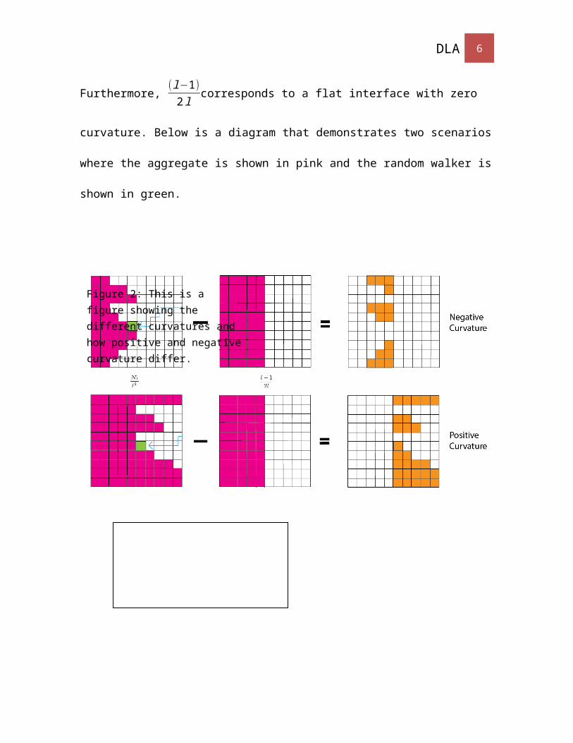
l2 value corresponds to positive curvature. Furthermore, (l−1)
2 l
corresponds to a flat interface with zero curvature. Below is a diagram that demonstrates
two scenarios where the aggregate is shown in pink and the random walker is shown in
green.
DLA 5
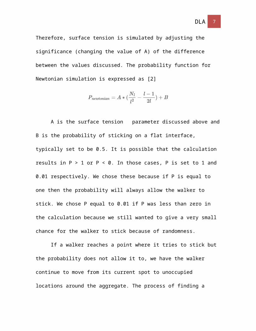
Therefore, surface tension is simulated by adjusting the significance (changing the value of
A) of the difference between the values discussed. The probability function for Newtonian
simulation is expressed as [2]
A is the surface tension parameter discussed above and B is the probability of
sticking on a flat interface, typically set to be 0.5. It is possible that the calculation results in
P > 1 or P < 0. In those cases, P is set to 1 and 0.01 respectively. We chose these because if
P is equal to one then the probability will always allow the walker to stick. We chose P
equal to 0.01 if P was less than zero in the calculation because we still wanted to give a
very small chance for the walker to stick because of randomness.
If a walker reaches a point where it tries to stick but the probability does not allow it
to, we have the walker continue to move from its current spot to unoccupied locations
around the aggregate. The process of finding a neighbor and calculating the sticking
probability is then repeated until the walker is able to stick or is discarded (discussed later).
As the value of “A” is increased the viscous fingers get thicker, whereas a smaller
value of “A” leads to more branches and skinnier fingers. This random process by itself
generates structures with holes of various sizes, which is not observed in experiments and
unrealistic. To prevent holes, each time a walker is able to stick at a point, we run a check
Figure 2: This is a figure showing the different curvatures and how positive and negative curvature differ.
DLA 6
to make sure that having the walker at this location will not create a hole. To do this, all
possible configurations around the particle that could lead to formation of a hole in a 3x3
box are considered. By induction, this method prevents holes of larger sizes.
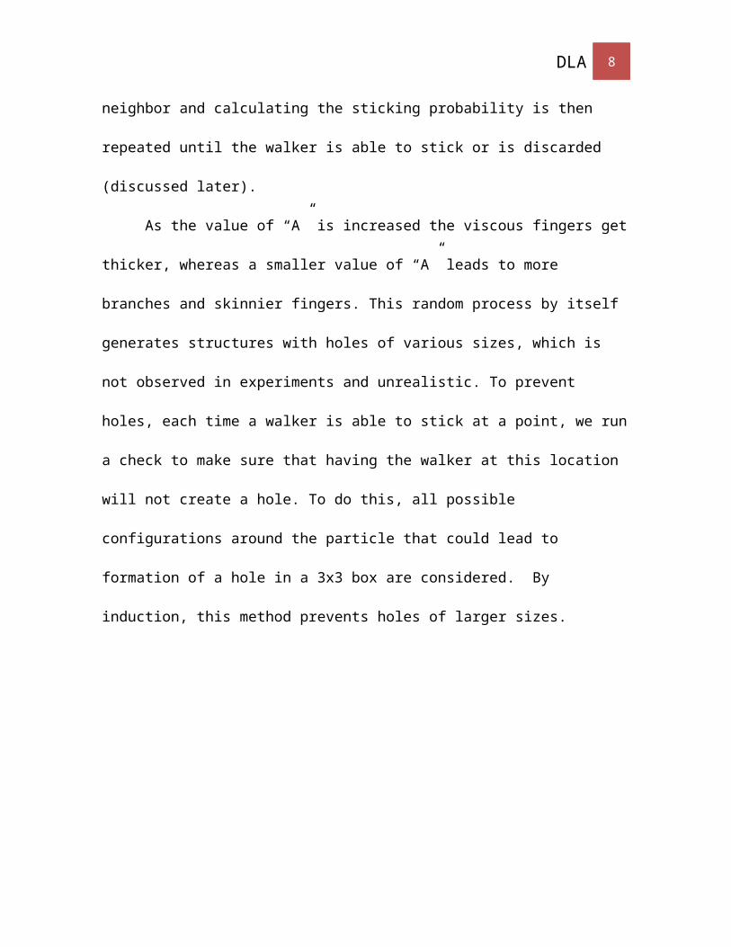
Based on the figure above, if the walker moves just the right way and attempts to
stick at the location of the gold space, this will create a hole. In our code, we have the
walker perform a check after each time it reaches a stuck walker. The function is called
holepreventTJ and essentially checks the number of neighbors to see if the new walker will
create a hole if it sticks there. The walker cannot have 4 neighbors because there is no way
it would have been able to move into such a location. If the number of neighbors is 3, then
the walker is fine to stick there because this location cannot form a hole no matter what. If
the number of neighbors is two, then the code will check if the neighbors are on opposite
sides of the walker. If this check proves true (the image above) the walker will not stick
there.
Figure 3: Shows a potential walker (pink) walking towards the aggregate (red).
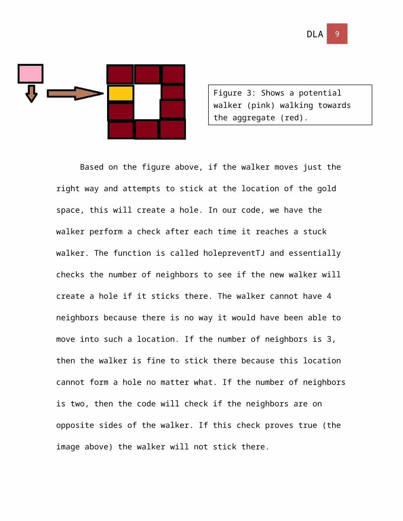
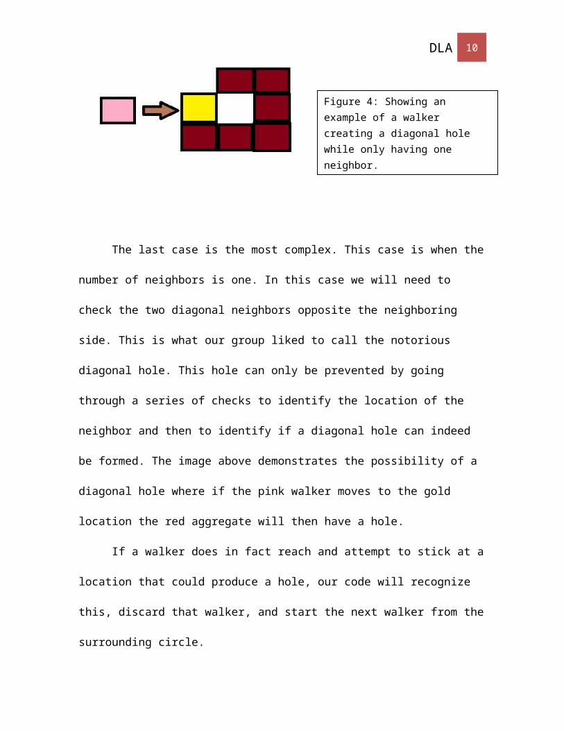
Figure 4: Showing an example of a walker creating a diagonal hole while only having one neighbor.
DLA 7
The last case is the most complex. This case is when the number of neighbors is
one. In this case we will need to check the two diagonal neighbors opposite the neighboring
side. This is what our group liked to call the notorious diagonal hole. This hole can only be
prevented by going through a series of checks to identify the location of the neighbor and
then to identify if a diagonal hole can indeed be formed. The image above demonstrates the
possibility of a diagonal hole where if the pink walker moves to the gold location the red
aggregate will then have a hole.
If a walker does in fact reach and attempt to stick at a location that could produce a
hole, our code will recognize this, discard that walker, and start the next walker from the
surrounding circle.
DLA 8
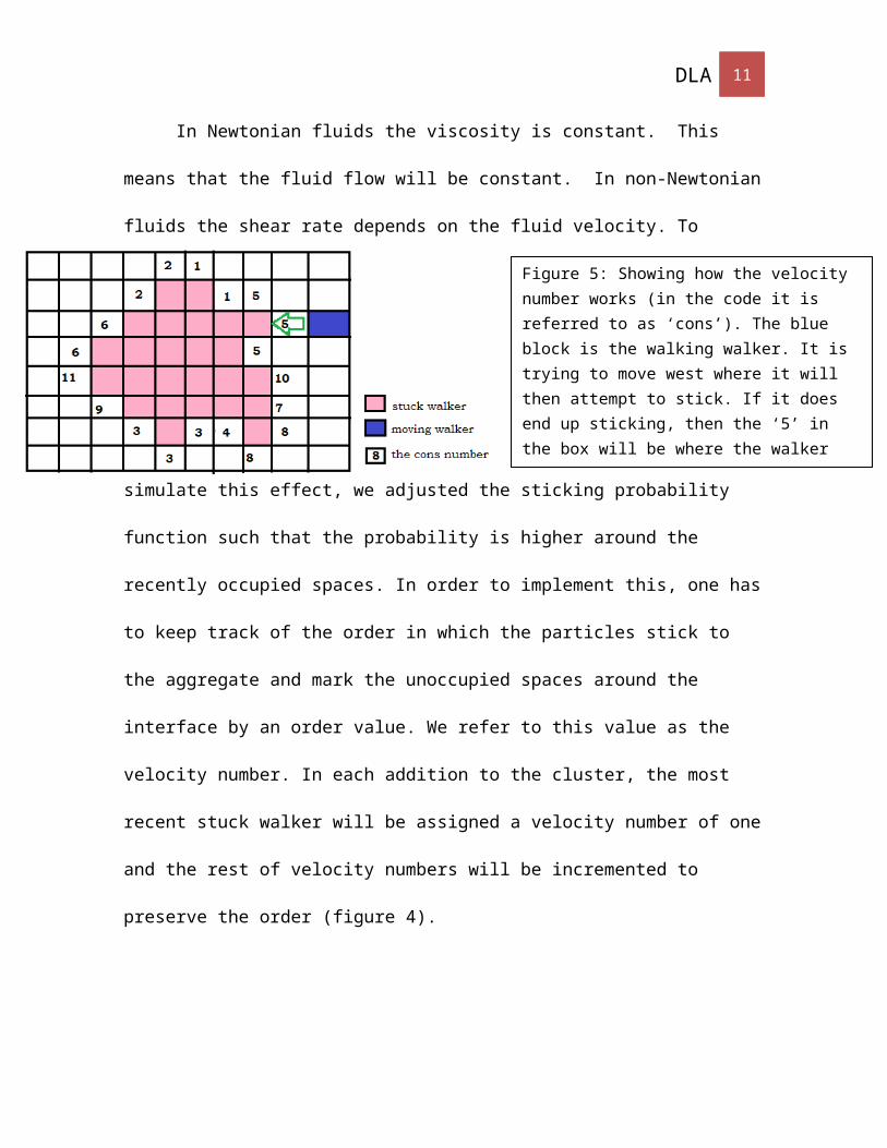
In Newtonian fluids the viscosity is constant. This means that the fluid flow will be
constant. In non-Newtonian fluids the shear rate depends on the fluid velocity. To simulate
this effect, we adjusted the sticking probability function such that the probability is higher
around the recently occupied spaces. In order to implement this, one has to keep track of
the order in which the particles stick to the aggregate and mark the unoccupied spaces
around the interface by an order value. We refer to this value as the velocity number. In
each addition to the cluster, the most recent stuck walker will be assigned a velocity
number of one and the rest of velocity numbers will be incremented to preserve the order
(figure 4).
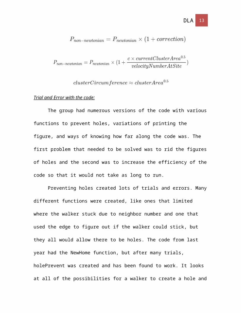
If the walker lands on the aggregate at a point where the velocity number is low, the
probability of sticking is larger. Therefore, this local value at the point where the walker
wants to stick appears in the denominator of the correction (see probability function below).
Furthermore, as the aggregate grows, the probability to stick on any spot on the interface
gets smaller, simply because there are more spots to stick. All unoccupied spots, around the
interface are approximately equal to the circumference of the cluster. However, calculating
the circumference of a structure each time a particle attempts to stick with fractal properties
Figure 5: Showing how the velocity number works (in the code it is referred to as ‘cons’). The blue block is the walking walker. It is trying to move west where it will then attempt to stick. If it does end up sticking, then the ‘5’ in the box will be where the walker sticks and the three boxes North, South, and East will then have a cons= 1 and every other cons number will increase by 1 (the highest number will then be 12).
DLA 9
is a difficult task. Therefore, we assume that the circumference is roughly equal to the
square root of the cluster area. In other words, we assume the cluster is a circle for this
calculation. This value appears on the numerator of the correction as shown below. Overall,
we expect the correction to create the desired effect to simulate Non-Newtonian fluid flow
[3].
Trial and Error with the code:
The group had numerous versions of the code with various functions to prevent
holes, variations of printing the figure, and ways of knowing how far along the code was.
The first problem that needed to be solved was to rid the figures of holes and the second
was to increase the efficiency of the code so that it would not take as long to run.
Preventing holes created lots of trials and errors. Many different functions were
created, like ones that limited where the walker stuck due to neighbor number and one that
used the edge to figure out if the walker could stick, but they all would allow there to be
holes. The code from last year had the NewHome function, but after many trials,
holePrevent was created and has been found to work. It looks at all of the possibilities for a
walker to create a hole and hinders the walker to stick there. The next question that needed
DLA 10
to be answered was if a walker would ever be discarded and not allowed to stick. There
ended up being three possibilities: 1) any walker that did not have a passing p-value would
not stick and the code would move on to the next walker, 2) if a walker had a failing p-
value, it would start to move again until it found a passing p-value, but if it failed to pass
holePrevent, it would not stick and the next walker would start, and 3) all of the walkers
would stick, so if a walker received a failing p-value or would have caused a hole according
to holePrevent, the walker would try moving again until it was allowed to stick. After
running many simulations, we decided to go with option (2) because it did not seem to
make much of a difference between the three situations and option (2) seemed like a happy
medium because most walkers still stuck. When running a simulation of 100,000
consistently more than 97% of the walkers would stick.
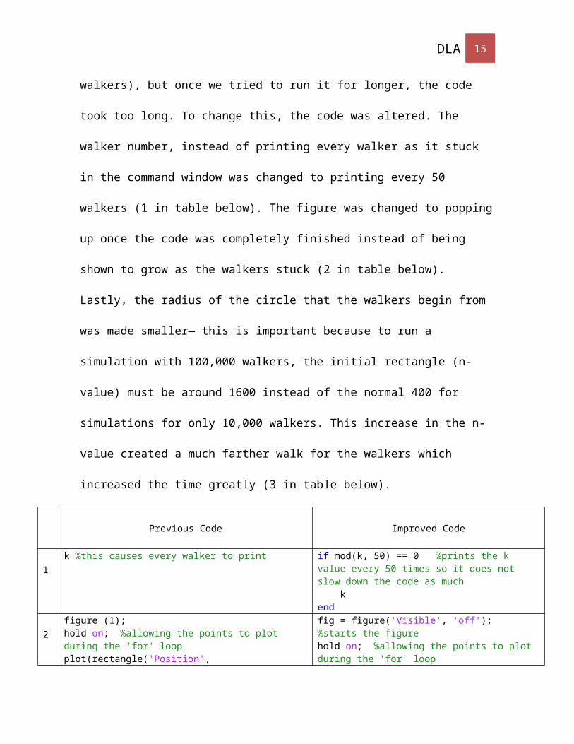
Once those issues were solved, the code took a reasonable time to run for shorter
simulations (about 10,000 walkers), but once we tried to run it for longer, the code took too
long. To change this, the code was altered. The walker number, instead of printing every
walker as it stuck in the command window was changed to printing every 50 walkers (1 in
table below). The figure was changed to popping up once the code was completely finished
instead of being shown to grow as the walkers stuck (2 in table below). Lastly, the radius of
the circle that the walkers begin from was made smaller— this is important because to run a
simulation with 100,000 walkers, the initial rectangle (n-value) must be around 1600
instead of the normal 400 for simulations for only 10,000 walkers. This increase in the n-
value created a much farther walk for the walkers which increased the time greatly (3 in
table below).
Previous Code Improved Code
DLA 11
1k %this causes every walker to print if mod(k, 50) == 0 %prints the k
value every 50 times so it does not slow down the code as much kend
2figure (1);hold on; %allowing the points to plot during the 'for' loop plot(rectangle('Position',[xo,yo,1,1],'FaceColor','m')); %makes the rectangles on the plot so the results can be seen with greater easedrawnow; %making it so you can see as the walkers stick
fig = figure('Visible', 'off'); %starts the figurehold on; %allowing the points to plot during the 'for' loop plot(rectangle('Position',[xo,yo,1,1],'FaceColor','m')); %makes the rectangles on the plot so the results can be seen with greater easedrawnow; %making it so you can see as the walkers stick…set(fig, 'visible', 'on');
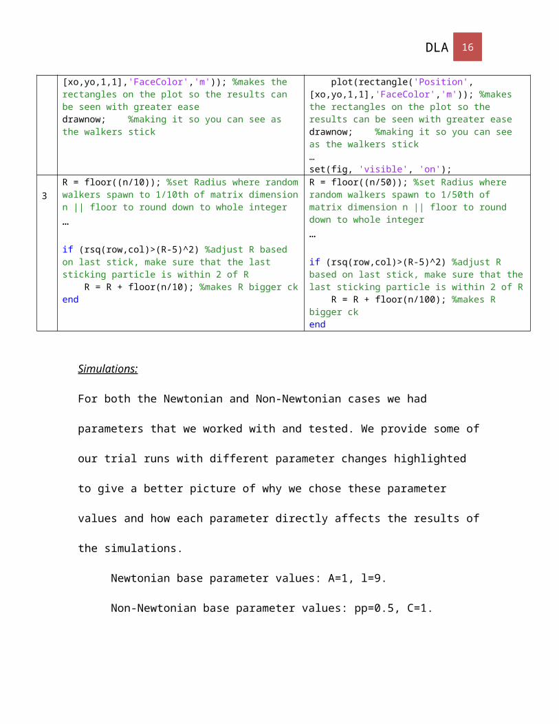
3R = floor((n/10)); %set Radius where random walkers spawn to 1/10th of matrix dimension n || floor to round down to whole integer…
if (rsq(row,col)>(R-5)^2) %adjust R based on last stick, make sure that the last sticking particle is within 2 of R R = R + floor(n/10); %makes R bigger ckend
R = floor((n/50)); %set Radius where random walkers spawn to 1/50th of matrix dimension n || floor to round down to whole integer…
if (rsq(row,col)>(R-5)^2) %adjust R based on last stick, make sure that the last sticking particle is within 2 of R R = R + floor(n/100); %makes R bigger ckend
Simulations:
For both the Newtonian and Non-Newtonian cases we had parameters that we worked with
and tested. We provide some of our trial runs with different parameter changes highlighted
to give a better picture of why we chose these parameter values and how each parameter
directly affects the results of the simulations.
Newtonian base parameter values: A=1, l=9.
Non-Newtonian base parameter values: pp=0.5, C=1.
Each figure was run for 10,000 walkers and the yellow highlight means this is the base
values of parameter.
DLA 12
Fluid A pp C Results
Non-
Newtonian
1.5 0.5 0.7
100 150 200 250 300
100
150
200
250
300
Non-Newtonian Fluid
x axis
y ax
is
Non-Newtonian 1 0.5 1
350 400 450 500 550 600 650
350
400
450
500
550
600
650
Non-Newtonian Fluid
x axis
y ax
is
DLA 13
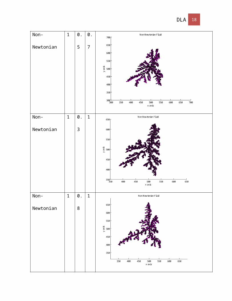
Non-Newtonian 1 0.5 0.7
300 350 400 450 500 550 600 650 700300
350
400
450
500
550
600
650
700Non-Newtonian Fluid
x axisy
axis
Non-Newtonian 1 0.3 1
350 400 450 500 550 600 650350
400
450
500
550
600
650Non-Newtonian Fluid
x axis
y ax
is
Non-Newtonian 1 0.8 1
350 400 450 500 550 600 650
350
400
450
500
550
600
650
Non-Newtonian Fluid
x axis
y ax
is
DLA 14
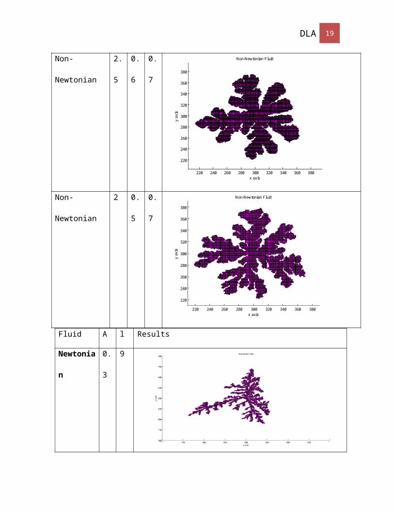
Non-Newtonian 2.5 0.6 0.7
220 240 260 280 300 320 340 360 380
220
240
260
280
300
320
340
360
380
Non-Newtonian Fluid
x axisy
axis
Non-Newtonian 2 0.5 0.7
220 240 260 280 300 320 340 360 380
220
240
260
280
300
320
340
360
380
Non-Newtonian Fluid
x axis
y ax
is
DLA 15
Fluid A l Results
Newtonian 0.3 9
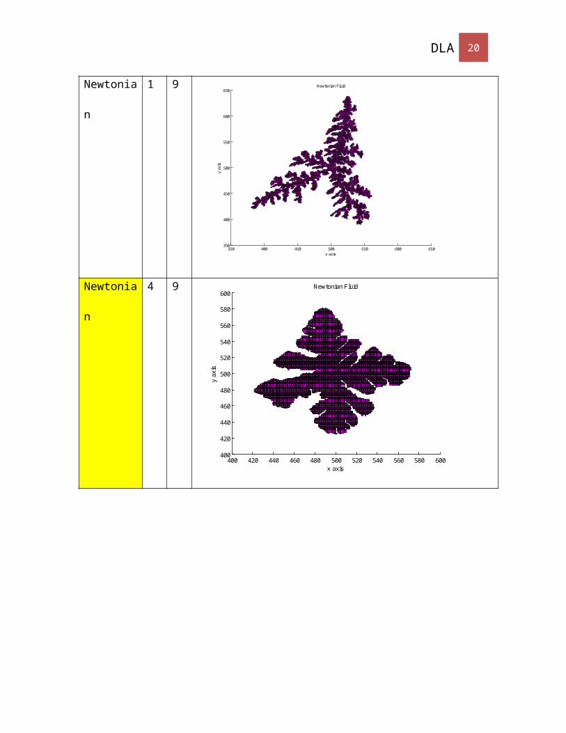
Newtonian 1 9
350 400 450 500 550 600 650350
400
450
500
550
600
650Newtonian Fluid
x axis
y ax
is
Newtonian 4 9
400 420 440 460 480 500 520 540 560 580 600400
420
440
460
480
500
520
540
560
580
600Newtonian Fluid
x axis
y ax
is
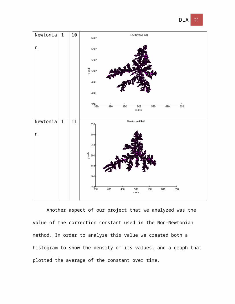
Newtonian 1 10
350 400 450 500 550 600 650350
400
450
500
550
600
650Newtonian Fluid
x axis
y ax
is
300 350 400 450 500 550 600 650 700300
350
400
450
500
550
600
650
700Newtonian Fluid
x axis
y ax
is
DLA 16
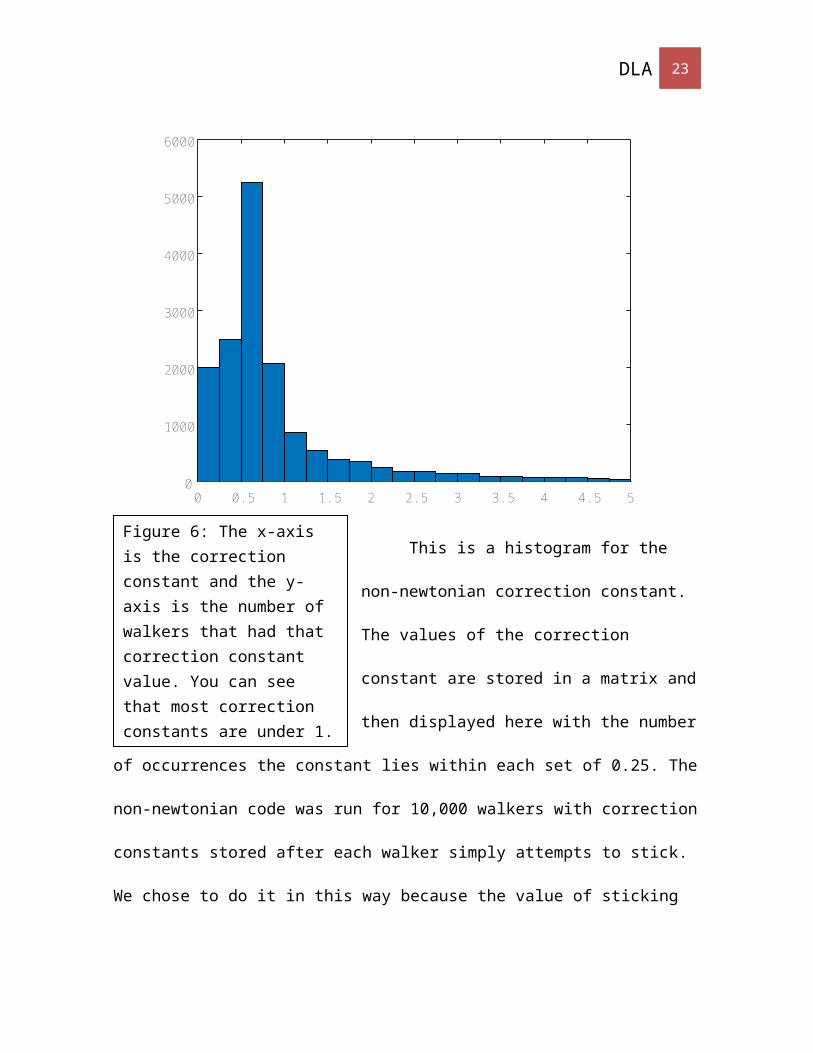
Another aspect of our project that we analyzed was the value of the correction
constant used in the Non-Newtonian method. In order to analyze this value we created both
a histogram to show the density of its values, and a graph that plotted the average of the
constant over time.
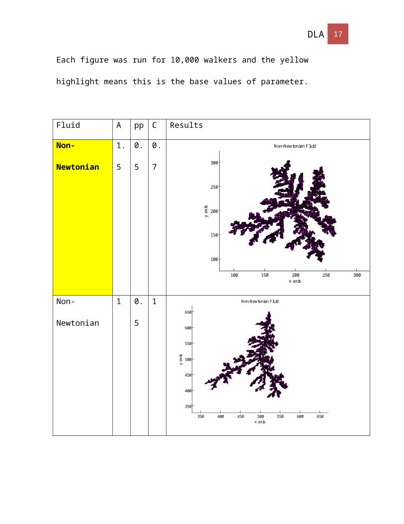
Figure 6: The x-axis is the correction constant and the y-axis is the number of walkers that had that correction constant value. You can see that most correction constants are under 1.
DLA 17
This is a histogram for the non-newtonian
correction constant. The values of the correction
constant are stored in a matrix and then displayed
here with the number of occurrences the constant lies
within each set of 0.25. The non-newtonian code was run for 10,000 walkers with
correction constants stored after each walker simply attempts to stick. We chose to do it in
this way because the value of sticking and not sticking both affect the image for non-
newtonian and therefore included all the calculated values.
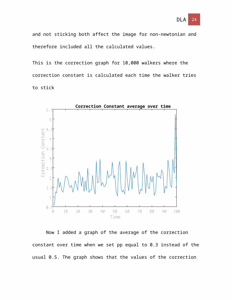
This is the correction graph for 10,000 walkers where the correction constant is calculated
each time the walker tries to stick
0 0.5 1 1.5 2 2.5 3 3.5 4 4.5 50
1000
2000
3000
4000
5000
6000
DLA 18
Time0 10 20 30 40 50 60 70 80 90 100
Cor
rect
ion
Con
stan
t
0.5
1
1.5
2
2.5
3
3.5
4
4.5
5
5.5Correction Constant average over time
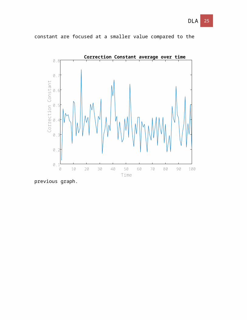
Now I added a graph of the average of the correction constant over time when we
set pp equal to 0.3 instead of the usual 0.5. The graph shows that the values of the
correction constant are focused at a smaller value compared to the previous graph.
DLA 19
Time0 10 20 30 40 50 60 70 80 90 100
Cor
rect
ion
Con
stan
t
0.1
0.2
0.3
0.4
0.5
0.6
0.7
0.8Correction Constant average over time
DLA 20
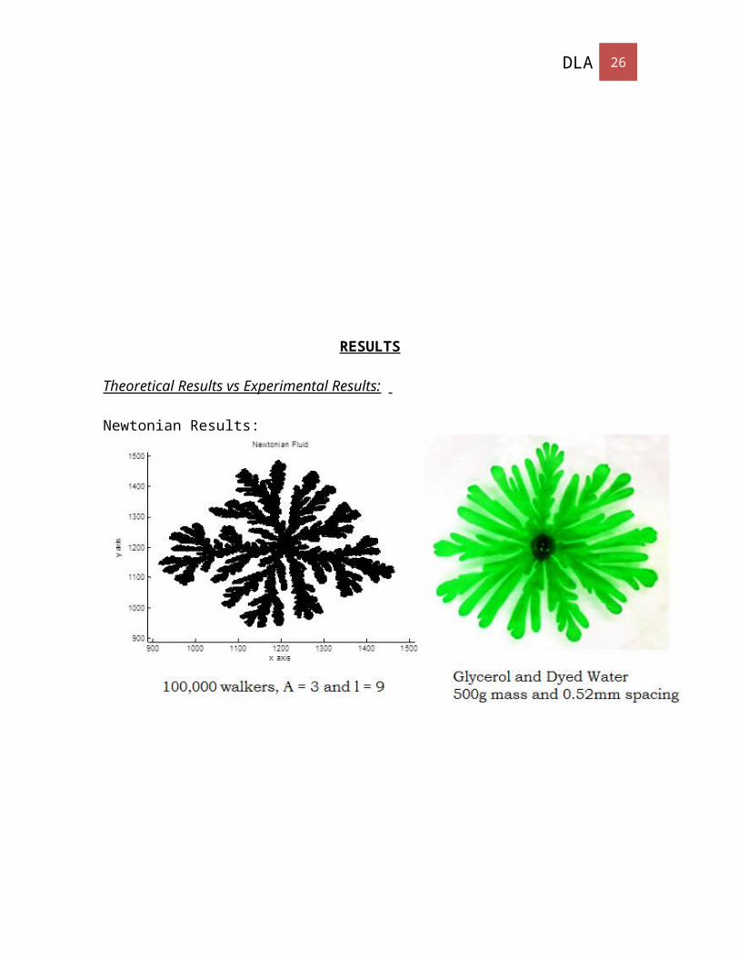
RESULTS
Theoretical Results vs Experimental Results:
Newtonian Results:
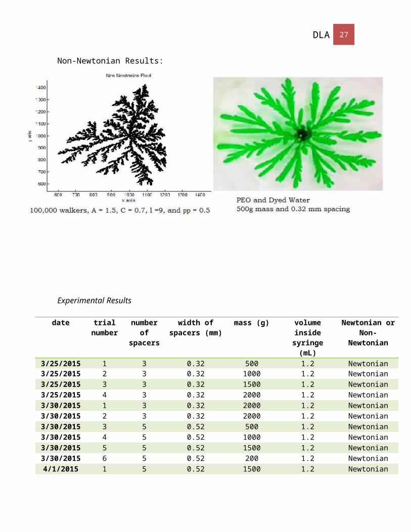
Non-Newtonian Results:
DLA 21
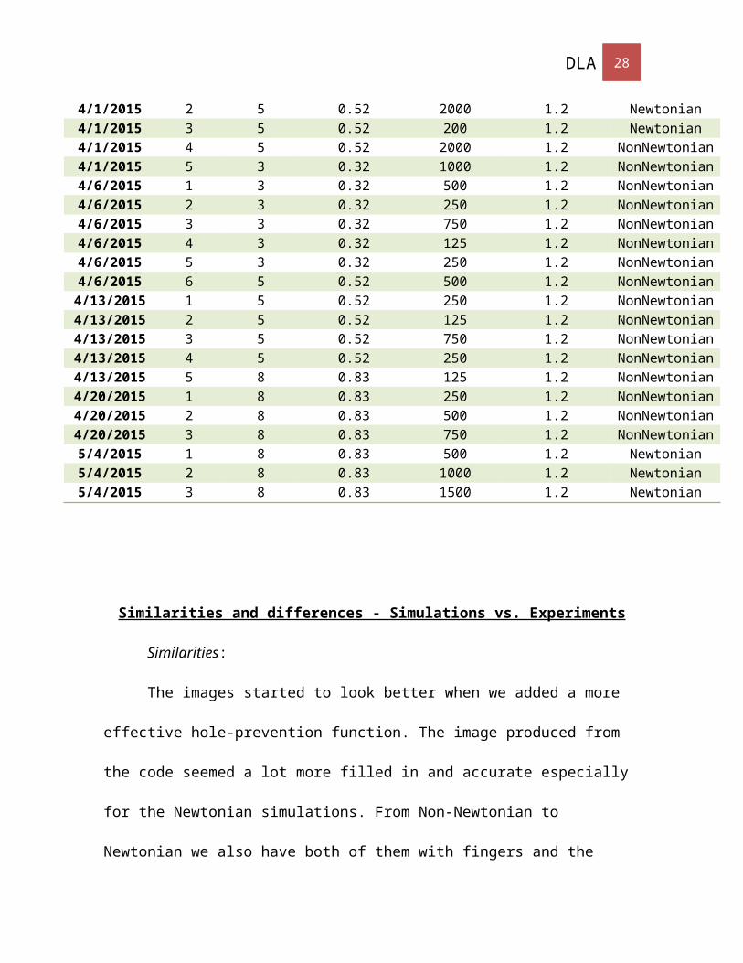
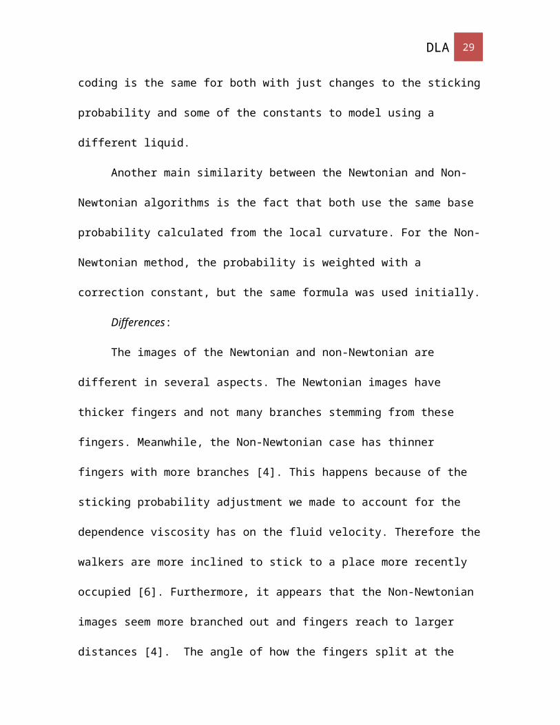
Experimental Results
date trial number
number of spacers
width of spacers (mm)
mass (g) volume inside syringe (mL)
Newtonian or Non-Newtonian
3/25/2015 1 3 0.32 500 1.2 Newtonian3/25/2015 2 3 0.32 1000 1.2 Newtonian3/25/2015 3 3 0.32 1500 1.2 Newtonian3/25/2015 4 3 0.32 2000 1.2 Newtonian3/30/2015 1 3 0.32 2000 1.2 Newtonian3/30/2015 2 3 0.32 2000 1.2 Newtonian3/30/2015 3 5 0.52 500 1.2 Newtonian3/30/2015 4 5 0.52 1000 1.2 Newtonian3/30/2015 5 5 0.52 1500 1.2 Newtonian3/30/2015 6 5 0.52 200 1.2 Newtonian4/1/2015 1 5 0.52 1500 1.2 Newtonian4/1/2015 2 5 0.52 2000 1.2 Newtonian4/1/2015 3 5 0.52 200 1.2 Newtonian4/1/2015 4 5 0.52 2000 1.2 NonNewtonian4/1/2015 5 3 0.32 1000 1.2 NonNewtonian4/6/2015 1 3 0.32 500 1.2 NonNewtonian4/6/2015 2 3 0.32 250 1.2 NonNewtonian4/6/2015 3 3 0.32 750 1.2 NonNewtonian4/6/2015 4 3 0.32 125 1.2 NonNewtonian4/6/2015 5 3 0.32 250 1.2 NonNewtonian4/6/2015 6 5 0.52 500 1.2 NonNewtonian4/13/2015 1 5 0.52 250 1.2 NonNewtonian4/13/2015 2 5 0.52 125 1.2 NonNewtonian4/13/2015 3 5 0.52 750 1.2 NonNewtonian4/13/2015 4 5 0.52 250 1.2 NonNewtonian4/13/2015 5 8 0.83 125 1.2 NonNewtonian4/20/2015 1 8 0.83 250 1.2 NonNewtonian4/20/2015 2 8 0.83 500 1.2 NonNewtonian4/20/2015 3 8 0.83 750 1.2 NonNewtonian5/4/2015 1 8 0.83 500 1.2 Newtonian5/4/2015 2 8 0.83 1000 1.2 Newtonian5/4/2015 3 8 0.83 1500 1.2 Newtonian
DLA 22
Similarities and differences - Simulations vs. Experiments
Similarities:
The images started to look better when we added a more effective hole-prevention
function. The image produced from the code seemed a lot more filled in and accurate
especially for the Newtonian simulations. From Non-Newtonian to Newtonian we also have
both of them with fingers and the coding is the same for both with just changes to the
sticking probability and some of the constants to model using a different liquid.
Another main similarity between the Newtonian and Non-Newtonian algorithms is
the fact that both use the same base probability calculated from the local curvature. For the
Non-Newtonian method, the probability is weighted with a correction constant, but the
same formula was used initially.
Differences:
The images of the Newtonian and non-Newtonian are different in several aspects.
The Newtonian images have thicker fingers and not many branches stemming from these
fingers. Meanwhile, the Non-Newtonian case has thinner fingers with more branches [4].
This happens because of the sticking probability adjustment we made to account for the
dependence viscosity has on the fluid velocity. Therefore the walkers are more inclined to
stick to a place more recently occupied [6]. Furthermore, it appears that the Non-Newtonian
images seem more branched out and fingers reach to larger distances [4]. The angle of how
the fingers split at the tips seem to be much more severe for non-Newtonian than for
Newtonian [6]. Non- Newtonian split at sharp angles rather than the rounded splitting of
Newtonian.
DLA 23
The simulated and experimental images for the Newtonian method are actually
quite similar. When we changed the value of A to 3 it really helped the image of the
Newtonian simulation look more like that of the experimental results. The fingers were
visually thicker to match that of the green images.
As for the Non-Newtonian images, the simulations still appeared to have thinner
fingers than that of the experimental images. Even with different variations in A, it did not
match as well as the Newtonian images did.
Fractal Dimension
Forms created between two liquids interacting have their shape effected by surface
tension. Randomly branched and sparse clusters are created in a wagon wheel spoke shape
as the two fluids interact with each other. As time continues the fingers formed will
randomly split and grow into less dense branch clusters. These created structures are in fact
fractals. Fractals are created when there is recursion [5]. It is a complex shape or pattern
that occurs as founding shape is repeated at different scale size during the picture [6].
Fractal dimension analysis helps us to examine shapes at different scales of size. To be
specific it measures the exact amount of space filled by the image. This can then be easily
compared to images in the same space. A Hausdorff dimension in particular measures the
size of an object while taking into account the fact that there is infinite numbers between
two endpoints [2]. It is show when parameters N=sd where d=ln N/ Ln s. In a Hele-Shaw
experiment fractional dimensions have been shown to be 1.70+/-0.05. This calculation is
not dependent on the flow rate or polymer concentration [6].
As the fluids interact there will only ever be growth on the tips of the clusters [8].
There will successive irregular splitting of the finger tips [6]. We are using wax paper to
DLA 24
try to reduce the tendency for liquid to form pools. This would complicate calculations for
fractal dimensions since the pooling in the middle would create more of a disk shape than
the fingers jutting out. Keeping the distance between the plates small on our experiments
will reduce air bubbles.
To compute the fractal dimensions on the theoretical results we are using a
computer code shown below. It is a function that pads the image with background pixels so
that the dimensions are a power of 2. The image is then sized (e). The function is then able
to count the number of boxes that contain one pixel from the image that is formed. The
points log (N(e))x log(1/e) and uses the least squared method to fit a line to the points. The
slope of the line computed is then the Haussdorf fractal dimension [2].
In computing the experimental fractal analysis we will use the high resolution video
taken with the experiment will be done. This video will then be imported into Matlab using
the video import file below. Each video is evaluated for its best beginning and ending
frame. The videos taken extend to when the dyed substances run over the circumference
where the first fluid is located. The last usable shot is several frames before the liquid
overflows. The first usable shot is the frame where a shape begins to form. To see the
change over time select ten frames evenly spaced between the usable images. Each image
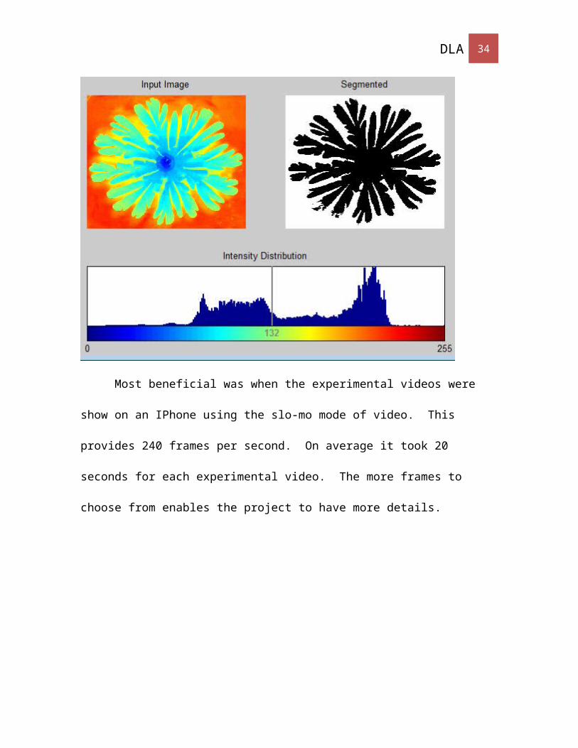
is then cropped to contain just the image, converted to black and white, and a threshold is
chosen that maintains the integrity of the image with the most detailing possible. This
required several trial and errors with a little bit of artistry. If the threshold is moved too
low detail is loss on the outermost fingers. However if it is too high the injection point of
dye at the center will be too large and not accurately reflect the image produced. This is
done with the video import file below.
DLA 25
Most beneficial was when the experimental videos were show on an IPhone using
the slo-mo mode of video. This provides 240 frames per second. On average it took 20
seconds for each experimental video. The more frames to choose from enables the project
to have more details.
DLA 26
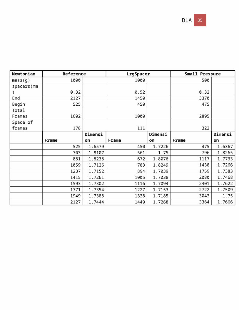
Newtonian Reference LrgSpacer Small Pressuremass(g) 1000 1000 500spacers(mm) 0.32 0.52 0.32End 2127 1450 3370Begin 525 450 475Total Frames 1602 1000 2895Space of frames 178 111 322
Frame Dimension Frame Dimension Frame Dimension525 1.6579 450 1.7226 475 1.6367703 1.8107 561 1.75 796 1.8265881 1.8238 672 1.8076 1117 1.7733
1059 1.7126 783 1.8249 1438 1.72661237 1.7152 894 1.7039 1759 1.73831415 1.7261 1005 1.7038 2080 1.74681593 1.7302 1116 1.7094 2401 1.76221771 1.7354 1227 1.7153 2722 1.75091949 1.7388 1338 1.7185 3043 1.752127 1.7444 1449 1.7268 3364 1.7666
0 500 1000 1500 2000 2500 3000 3500 40001.5
1.55
1.6
1.65
1.7
1.75
1.8
1.85
Newtonian Fractal Experimental Analysis Reference Small Pressure Large Spacing
Time (frames)
Frac
tal D
imen
sion
DLA 27
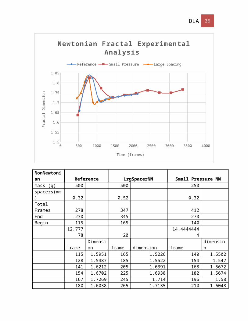
NonNewtonian Reference LrgSpacerNN Small Pressure NNmass (g) 500 500 250spacers(mm) 0.32 0.52 0.32Total Frames 278 347 412End 230 345 270Begin 115 165 140
12.77778 20 14.44444444
frameDimension frame dimension frame dimension
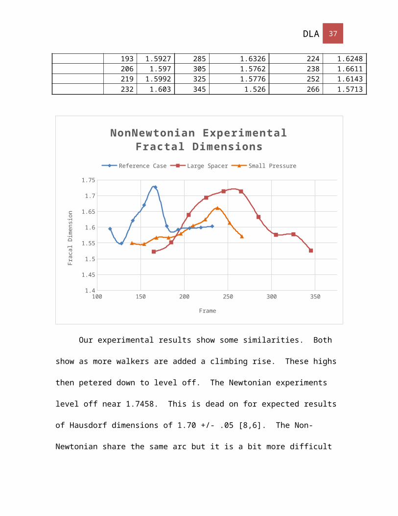
115 1.5951 165 1.5226 140 1.5502128 1.5487 185 1.5522 154 1.547141 1.6212 205 1.6391 168 1.5672154 1.6702 225 1.6938 182 1.5674167 1.7269 245 1.714 196 1.58180 1.6038 265 1.7135 210 1.6048193 1.5927 285 1.6326 224 1.6248206 1.597 305 1.5762 238 1.6611219 1.5992 325 1.5776 252 1.6143232 1.603 345 1.526 266 1.5713
DLA 28
100 150 200 250 300 3501.4
1.45
1.5
1.55
1.6
1.65
1.7
1.75
NonNewtonian Experimental Fractal Di-mensions
Reference Case Large Spacer Small Pressure
Frame
Frac
al D
imen
sion
Our experimental results show some similarities. Both show as more walkers are
added a climbing rise. These highs then petered down to level off. The Newtonian
experiments level off near 1.7458. This is dead on for expected results of Hausdorf
dimensions of 1.70 +/- .05 [8,6]. The Non-Newtonian share the same arc but it is a bit
more difficult to pinpoint the ending off point. Their last frame dimension results average
to 1.5667. Non-Newtonian expectations from last year are expected to be near 1.60 +/-.05.
These smaller dimensions can be explained because the crystals that form keep the image
created smaller and more compact than the sprawling Newtonian image.
In Newtonian the videos differed between all the different parameters for good
reason. The video frames chosen never lines up because growth is so different with
changing parameters. Small pressure achieved the highest density because it maintained
DLA 29
the smaller .32 mm plate separation. Large spacing with 1000 mg of pressure showed the
lowest amount of growth. However the symmetry remained in all experiments.
Non-Newtonian garnered some interesting experimental results. The reference
curve maintained the arc previously mentioned up growth and gradual decay to a point.
However the large spacing produce more of a bell curved shape. The small pressure
showed a spiky rise and sharp decline to a sudden stop. These varied results could be
attributed to the lack of slow-mo recording. There was less frames to choose from so any
change that occurred was much more sudden than it was gradual.
Simulations results of fractal dimensions were easier to complete. Inserted into our
already completed code without holes was the hausDim file. A plot was added to track the
dimension as the image grew. Initially we thought running the simulation for 10,000
walkers would near us to the desired 1.70 +/- 0.05 in Newtonian. However it did not. We
then expanded to evaluating at 100,000 walkers. While the images are listed on page 19 of
this paper, below is the graph showing growth. The code took somewhere near 6 hours to
run and the highest fractal dimension recorded was 1.4765.
DLA 30
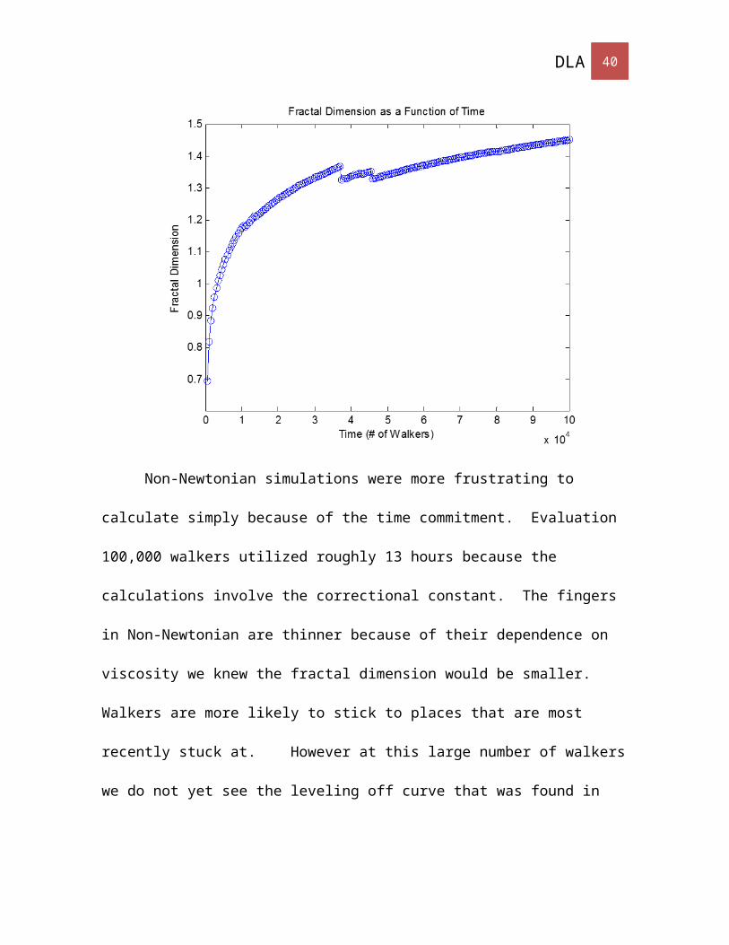
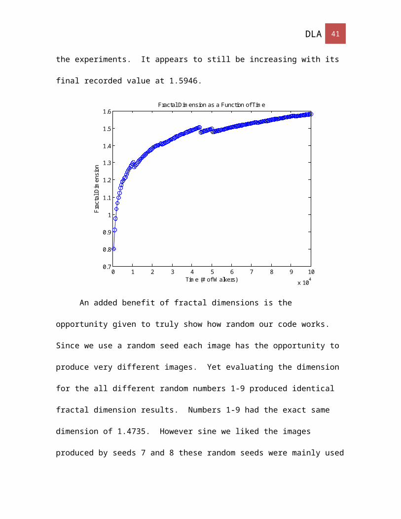
Non-Newtonian simulations were more frustrating to calculate simply because of
the time commitment. Evaluation 100,000 walkers utilized roughly 13 hours because the
calculations involve the correctional constant. The fingers in Non-Newtonian are thinner
because of their dependence on viscosity we knew the fractal dimension would be smaller.
Walkers are more likely to stick to places that are most recently stuck at. However at this
large number of walkers we do not yet see the leveling off curve that was found in the
experiments. It appears to still be increasing with its final recorded value at 1.5946.
DLA 31
0 1 2 3 4 5 6 7 8 9 10
x 104
0.7
0.8
0.9
1
1.1
1.2
1.3
1.4
1.5
1.6Fractal Dimension as a Function of Time
Time (# of Walkers)
Frac
tal D
imen
sion
An added benefit of fractal dimensions is the opportunity given to truly show how
random our code works. Since we use a random seed each image has the opportunity to
produce very different images. Yet evaluating the dimension for the all different random
numbers 1-9 produced identical fractal dimension results. Numbers 1-9 had the exact same
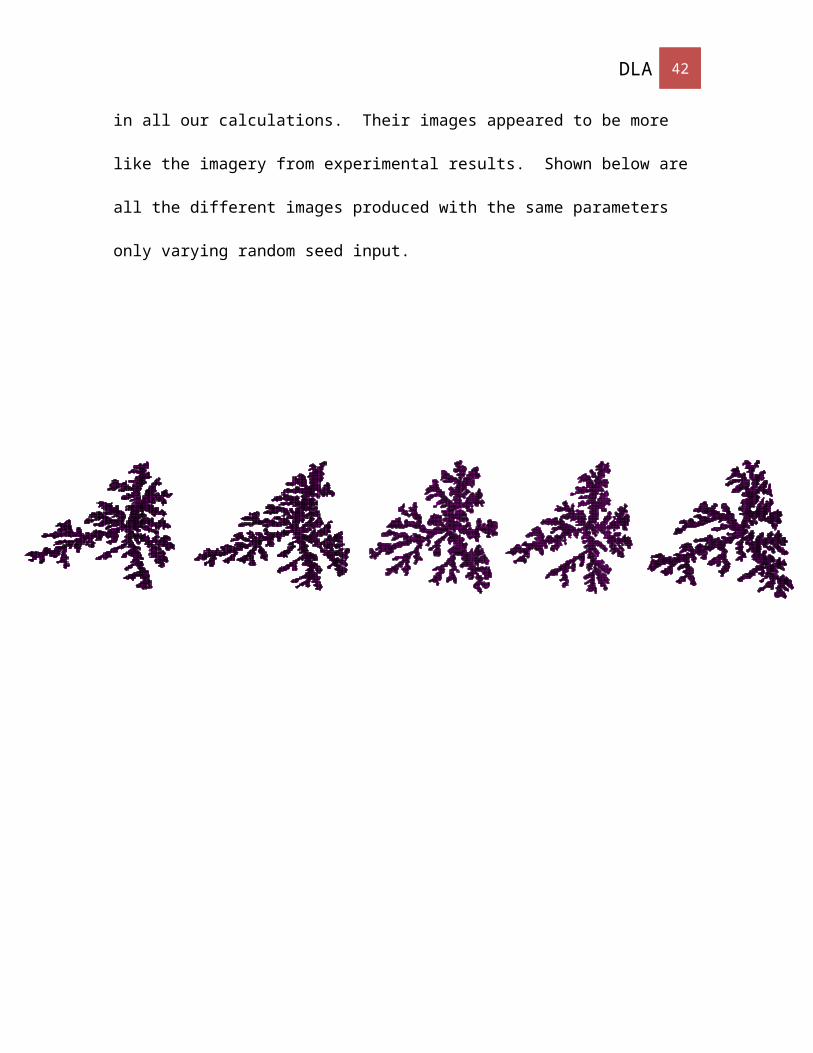
dimension of 1.4735. However sine we liked the images produced by seeds 7 and 8 these
random seeds were mainly used in all our calculations. Their images appeared to be more
like the imagery from experimental results. Shown below are all the different images
produced with the same parameters only varying random seed input.
DLA 32
100 150 200 250 300
100
150
200
250
300
Newtonian Fluid
x axis
y ax
is
100 150 200 250 300
100
150
200
250
300
Newtonian Fluid
x axis
y ax
is
100 120 140 160 180 200 220 240 260 280 300
100
120
140
160
180
200
220
240
260
280
300
Newtonian Fluid
x axis
y ax
is
100 150 200 250 300
100
150
200
250
300
Newtonian Fluid
x axis
y ax
is
100 150 200 250 300
100
150
200
250
300
Newtonian Fluid
x axis
y ax
is
DLA 33
A semester spent studying the one topic of DLA was very beneficial. It
involved working together as a team to solve a difficult problem from the ground up in a
way that had not been expected before in other classes. Learning from our experience there
are some suggestions for next years’ group to have their project go smoothly. The group
will be given our code the same as we received 2014 code. However it is critical to have a
solid understanding of the differences between the Newtonian and Non-Newtonian methods
before starting to code. Our code could stand to be improved regarding running times. The
Non-Newtonian code requires on average 15 hours to run 100,000 walkers. Each detail
restricting the movement is spelled out in the code. However maybe there is a way the
computer could check everything faster. It was discovered that for some reason running it
as a movie code sped the process up significantly. This only required 6 hours.
Another area that could stand some improvement is in larger simulations. At higher
number of walkers it appears that there are holes. Zooming in reveals that they are actually
just extremely narrow channels created and not actually holes. However in comparison
with experiments there should not be these extremely narrow channels. There should be a
way to fix this. In relation to the experiment as well the simulations do not maintain the
same symmetrical shape. Certain seeds tended to grow fingers in one particular direction.
If possible this should be addressed.
In the beginning our group struggled to understand exactly why parameter changes
effected the simulations. It would like better or worse depending on the A, l, c, pp
variables. Next year’s group should focus on these at the beginning so they can tell
whether the image is correctly showing what should be expecting from each variable
change. It is also important to have communication between DLA group and the
experimental group. The experimental group had to add on and redo certain steps to have
good comparing data for the simulation. It should be discussed beforehand exactly what
each team needs so that no time is waster.
Time also ran out on our group to be able to make further analysis of results.
Fractal dimension is hashed out but it would have been nice to have other values to
compare it with. We were unable to pin down wavelength analysis and density-density
100 150 200 250 300
100
150
200
250
300
Newtonian Fluid
x axis
y ax
is
100 150 200 250 300
100
150
200
250
300
Newtonian Fluid
x axis
y ax
is
100 150 200 250 300
100
150
200
250
300
Newtonian Fluid
x axis
y ax
is
100 120 140 160 180 200 220 240 260 280 300
100
120
140
160
180
200
220
240
260
280
300
Newtonian Fluid
x axis
y ax
is
DLA 34
correlation. Wavelengths involves tracking the boundary. Perhaps next year could utilize
code from the boundary integral group. Our boundary was identified but we were unable to
have the code pinpoint a start and end point so the complete area could be accurately
graphed. Density-density was difficult to graph regarding circular growth in a square
matrix of results. Overall this was a great learning experience and a fantastic year. We
wish next year’s graduation candidates well.
DLA 35
Newtonian Code:
function [Num_walk dimension] = SALTFunctionsNewtonianJULIA(n,num_part,A,B,l)%data = SALTFunctionsNewtonianJULIA(n,num_part,A,B,l)%n = the size of the rectangle that holds the circle%num_part= the amount of walkers you want, normally 10000%A = variable for probability, normally 1%B = variable for probability, normally 0.5%l = varible used to find local curvature, normally 9 %Muy Importante!!!!!!! If this is not commented out, then every time you run the code, it will have the same randomness, and make the same shape!!! s = RandStream('mcg16807','seed', 8); %to change to a different set randomness, change the last digit to something else RandStream.setGlobalStream(s); %comment this out too if want totally randomly different each time f = @(x,row) -2*x+row+1; %north and south: f=row+1 for south, f=row-1 for north || when a number is randomly generated, this function changes it into the correct movement: N or S g = @(x,col) -2*x+col+5; %west and east: g=col+1 for east g=col-1 for west || when a number is randomly generated, this function changes it into the correct movement: W or E fig = figure('Visible', 'off'); %starts the figure xo = floor(n/2); %center of circle (really finds the center of the square determined by the n value given to the function) yo = floor(n/2); %center of circle hold on; %allowing the points to plot during the 'for' loop plot(rectangle('Position',[xo,yo,1,1],'FaceColor','m')); %makes the rectangles on the plot so the results can be seen with greater ease drawnow; %making it so you can see as the walkers stick data = zeros(n,n,'int8'); %initializing data data(xo,yo,1) = 1; %making the first walker stick to the center rsq = @(x,y) (x-xo)^2+(y-yo)^2; %making the initial circle around the seed, using the equation for a circle R = floor((n/50)); %set Radius where random walkers spawn to 1/10th of matrix dimension n || floor to round down to whole integer dimension=[]; Num_walk = 0; for k = 1:num_part; %runs the function for the amount of walkers initally specified moveon = 0; if mod(k, 50) == 0 %prints the k value every 50 times so it does not slow down the code as much k
DLA 36
end theta =(2*pi)*rand; %modeled as a circle in first quadrant centered at (xo,yo) || rand randomly generates a number so each walker in theory will start from a different spot col = floor(xo+(R-1)*cos(theta)); %start the walker at a random position along the circle of radius R using the randomly generated theta value and the R value row = floor(yo+(R-1)*sin(theta)); columnflag = 0; %used to allow for a new walker to start walking while (columnflag == 0) move = randi([0 3],1,1); % 0 north 1 south 2 east 3 west, begin moving the walker randomly %returns a one-by-one matrix with a value of 0,1,2, or 3 which is later put into the g or f function above to determine which direction the walker is told to move occupiedflag = 0; if(move >= 2) %if walker is to be moved east or west (IE move= 2 or 3) check whether that "move" is ok to make (not equal to 1) if((rsq(row,g(move,col))< R^2) && (data(row, g(move,col))~= 1)) %make sure that move is not going to cross over our boundary determined by our R (Radius) value col = g(move,col); %make move if the walker will not move out of the circle else col = col; %if move not okay, then another randomly generated move is found end neigh = data(row,col+1) + data(row, col-1) + data(row-1,col) + data(row+1,col); %looking to see if the walker is next to a previously stuck walker if neigh >= 1 occupiedflag = 1; %if the walker is next to a stuck walker, then the 'if occupiedflag == 1' loop is begun and the walker has a chance of sticking there end else %if the move is south or north (0 or 1) check whether the move will be occupied if((rsq(f(move,row),col) < R^2)&&(data(f(move,row),col) ~= 1)) %make sure the move is not going to cross the circle determined by the Radius row = f(move,row); %make move else row = row; %if move not okay, then another randomly generated move is found end neigh = data(row,col+1) + data(row, col-1) + data(row-1,col) + data(row+1,col); %looking to see if the walker is next to a previously stuck walker
DLA 37
if neigh >= 1 occupiedflag = 1; %if the walker is next to a stuck walker, then the 'if occupiedflag == 1' loop is begun and the walker has a chance of sticking there end end if occupiedflag == 1 %we have reached the seed-- need to check the local curvature near the seed p = FindProb(data, row, col, A, B, l); %function used to determine the probability for the walker to stick where it is (takes in data, row, col, A, B, and l)(outputs p) if(rand <= p || p >= 1) %roll a dice (rand) and determine if walker sticks OR ( the '||' in the code ) if the proability is > 1 (high curvature) stick % if rand is greater than p, then that 'if' loop is broken, the occupied flag loop is broken, this walker will not stick and a new walker is begun [row, col] = NewHome(row,col,data);%function using a lxl box to count the number of 1s inside :kadanoff paper (http://m.njit.edu/~kondic/capstone/2014/vicsek_prl_84.pdf)(takes in row, col, and data)(returns col and row which might or might not have been updated) co = holePreventTJ(row, col, data); %function made to prevent holes using many conditionals (inputs row, col, and data)(outputs a value co, which is used below to determine whether the walker is allowed to stick or not) if co == 0; %the walker is finally allowed to stick Num_walk = Num_walk +1; columnflag = 1; % to break you out of the while loop so a new walker can start after this 'if' loop is finished data(row,col,1)=1; %walker has stuck (all spots where a walker has stuck have a value of '1', all other spots are '0') plot(rectangle('Position',[row,col,1,1],'FaceColor','m')); %plots that walker on the plot drawnow; title('Newtonian Fluid'); %adds the title to the graph xlabel('x axis'); %adds the x axis label to the graph ylabel('y axis'); %adds the y axis label to the graph axis([xo-R xo+R yo-R yo+R]); % makes the axises change according to how large the current Radius is (centered around the first walker) if (rsq(row,col)>(R-5)^2) %adjust R based on last stick, make sure that the last sticking particle is within 2 of R R = R + floor(n/100); %makes R bigger ck end else moveon = moveon + 1; end

DLA 38
if moveon >= 10 columnflag = 1; %does not allow that walker to stick because it got stuck end end end end if mod(k,500)==0, dimension(k/500,1)=k; dimension(k/500,2)=hausDim(data); end end figure(); plot(dimension(:,1),dimension(:,2),'-o'); title('Fractal Dimension as a Function of Time SEED=8'); xlabel('Time (# of Walkers)'); ylabel('Fractal Dimension'); figure(); plot(dimension(2:end,2)./dimension(1:(end-1),2),'-o'); title('Density Correlation as a Function of Time'); filename = sprintf('SALTFunctionsNewtonianJULIA(%d, %d, %g, %g, %g).fig', n, num_part, A, B, l); saveas(fig, filename); set(fig, 'visible', 'on');end
Published with MATLAB® R2014a
DLA 39
Newtonian Code to make Movies
function [Num_walk dimension] = SALTFunctionsNewtonianJULIAmovie(n,num_part,A,B,l)%data = SALTFunctionsNewtonianJULIAmovie(n,num_part,A,B,l)%n = the size of the rectangle that holds the circle%num_part= the amount of walkers you want, normally 10000%A = variable for probability, normally 1%B = variable for probability, normally 0.5%l = varible used to find local curvature, normally 9 filename = sprintf('movieNew(%d, %g, %g).avi', num_part, A, l); writerObj = VideoWriter(filename); open(writerObj); jj=1; %Muy Importante!!!!!!! If this is not commented out, then every time you run the code, it will have the same randomness, and make the same shape!!! s = RandStream('mcg16807','seed', 3); %to change to a different set randomness, change the last digit to something else RandStream.setGlobalStream(s); %comment this out too if want totally randomly different each time f = @(x,row) -2*x+row+1; %north and south: f=row+1 for south, f=row-1 for north || when a number is randomly generated, this function changes it into the correct movement: N or S g = @(x,col) -2*x+col+5; %west and east: g=col+1 for east g=col-1 for west || when a number is randomly generated, this function changes it into the correct movement: W or E xo = floor(n/2); %center of circle (really finds the center of the square determined by the n value given to the function) yo = floor(n/2); %center of circle data = zeros(n,n,'int8'); %initializing data data(xo,yo,1) = 1; %making the first walker stick to the center rsq = @(x,y) (x-xo)^2+(y-yo)^2; %making the initial circle around the seed, using the equation for a circle R = floor((n/50)); %set Radius where random walkers spawn to 1/10th of matrix dimension n || floor to round down to whole integer dimension=[]; Num_walk = 0; for k = 1:num_part; %runs the function for the amount of walkers initally specified moveon = 0; if mod(k, 50) == 0 %prints the k value every 50 times so it does not slow down the code as much k
DLA 40
end theta =(2*pi)*rand; %modeled as a circle in first quadrant centered at (xo,yo) || rand randomly generates a number so each walker in theory will start from a different spot col = floor(xo+(R-1)*cos(theta)); %start the walker at a random position along the circle of radius R using the randomly generated theta value and the R value row = floor(yo+(R-1)*sin(theta)); columnflag = 0; %used to allow for a new walker to start walking while (columnflag == 0) move = randi([0 3],1,1); % 0 north 1 south 2 east 3 west, begin moving the walker randomly %returns a one-by-one matrix with a value of 0,1,2, or 3 which is later put into the g or f function above to determine which direction the walker is told to move occupiedflag = 0; if(move >= 2) %if walker is to be moved east or west (IE move= 2 or 3) check whether that "move" is ok to make (not equal to 1) if((rsq(row,g(move,col))< R^2) && (data(row, g(move,col))~= 1)) %make sure that move is not going to cross over our boundary determined by our R (Radius) value col = g(move,col); %make move if the walker will not move out of the circle else col = col; %if move not okay, then another randomly generated move is found end neigh = data(row,col+1) + data(row, col-1) + data(row-1,col) + data(row+1,col); %looking to see if the walker is next to a previously stuck walker if neigh >= 1 occupiedflag = 1; %if the walker is next to a stuck walker, then the 'if occupiedflag == 1' loop is begun and the walker has a chance of sticking there end else %if the move is south or north (0 or 1) check whether the move will be occupied if((rsq(f(move,row),col) < R^2)&&(data(f(move,row),col) ~= 1)) %make sure the move is not going to cross the circle determined by the Radius row = f(move,row); %make move else row = row; %if move not okay, then another randomly generated move is found end neigh = data(row,col+1) + data(row, col-1) + data(row-1,col) + data(row+1,col); %looking to see if the walker is next to a previously stuck walker
DLA 41
if neigh >= 1 occupiedflag = 1; %if the walker is next to a stuck walker, then the 'if occupiedflag == 1' loop is begun and the walker has a chance of sticking there end end if occupiedflag == 1 %we have reached the seed-- need to check the local curvature near the seed p = FindProb(data, row, col, A, B, l); %function used to determine the probability for the walker to stick where it is (takes in data, row, col, A, B, and l)(outputs p) if(rand <= p || p >= 1) %roll a dice (rand) and determine if walker sticks OR ( the '||' in the code ) if the proability is > 1 (high curvature) stick % if rand is greater than p, then that 'if' loop is broken, the occupied flag loop is broken, this walker will not stick and a new walker is begun [row, col] = NewHome(row,col,data);%function using a lxl box to count the number of 1s inside :kadanoff paper (http://m.njit.edu/~kondic/capstone/2014/vicsek_prl_84.pdf)(takes in row, col, and data)(returns col and row which might or might not have been updated) co = holePrevent(row, col, data); %function made to prevent holes using many conditionals (inputs row, col, and data)(outputs a value co, which is used below to determine whether the walker is allowed to stick or not) if co == 0; %the walker is finally allowed to stick Num_walk = Num_walk +1; columnflag = 1; % to break you out of the while loop so a new walker can start after this 'if' loop is finished data(row,col,1)=1; %walker has stuck (all spots where a walker has stuck have a value of '1', all other spots are '0') if (rsq(row,col)>(R-5)^2) %adjust R based on last stick, make sure that the last sticking particle is within 2 of R R = R + floor(n/100); %makes R bigger ck end else moveon = moveon + 1; end if moveon >= 20 columnflag = 1; %does not allow that walker to stick because it got stuck end if mod(k,100)==1 colormap([0 0 0; 1 1 1 ]); image(data(:,:) .* 255); set(gca,'nextplot','replacechildren'); set(gcf,'Renderer','zbuffer'); M(jj)=getframe;
DLA 42
writeVideo(writerObj, M(jj)); jj=jj+1; end end end end if mod(k,500)==0, dimension(k/500,1)=k; dimension(k/500,2)=hausDim(data); end end figure(); plot(dimension(:,1),dimension(:,2),'-o'); title('Fractal Dimension as a Function of Time'); xlabel('Time (# of Walkers)'); ylabel('Fractal Dimension'); figure(); plot(dimension(2:end,2)./dimension(1:(end-1),2),'-o'); title('Density Correlation as a Function of Time'); close(writerObj);end
DLA 43
Non-Newtonian Code:
function [Num_walk data] = SALTNONNewtonianJULIAAR(n,num_part,A,l, pp, C)%data = SALTNONNewtonianJULIA(n,num_part,A,l, pp, C)%n = the size of the rectangle that holds the circle%num_part= the amount of walkers you want, normally 10000%A = variable for probability, normally 1%l = varible used to find local curvature, normally 9% pp is the exponent that k is raised to in the probability, normally 1/2%C is the velocity number used in probability, normally 1 %Muy Importante!!!!!!! If this is not commented out, then every time you run the code, it will have the same randomness, and make the same shape!!! s = RandStream('mcg16807','seed', 8); %to change to a different set randomness, change the last digit to something else RandStream.setGlobalStream(s); %comment this out too if want totally randomly different each time f=@(x,row) -2*x+row+1; %north and south: f=row+1 for south, f=row-1 for north || when a number is randomly generated, this function changes it into the correct movement: N or S g=@(x,col) -2*x+col+5; %west and east: g=col+1 for east g=col-1 for west || when a number is randomly generated, this function changes it into the correct movement: W or E fig = figure('Visible', 'off'); %starts the figure xo=floor(n/2); %center of circle (really finds the center of the square determined by the n value given to the function) yo=floor(n/2); %center of circle hold on; %allowing the points to plot during the for loop rectangle('Position',[xo yo 1 1],'FaceColor','m'); %makes the rectangles on the plot so the results can be seen with greater ease drawnow; %making it so you can see as they graph cons =zeros(n,n,'int8'); %initializing data data=zeros(n,n,'int8'); %initializing data data(xo,yo,1)=1; %making the first walker rsq=@(x,y) (x-xo)^2+(y-yo)^2; %making the initial circle around the seed, using the equation for a circle dimension=[]; Num_walk = 0; R=floor((n/50)); %set Radius where random walkers spawn to 1/10 th of matrix dimension n || floor to round down to whole integer for k=1:num_part;%runs the function for the amount of walkers initally specified moveon = 0; if mod(k, 50) == 0 %prints the k value every 50 times so it does not slow down the code as much k end
DLA 44
theta=(2*pi)*rand; %modeled as a circle in first quadrant centered at (xo,yo)|| rand randomly generates a number so each walker in theory will start from a different spot col=floor(xo+(R-1)*cos(theta)); %start the walker at a random position along the circle of radius R using the randomly generated theta value and the R value row=floor(yo+(R-1)*sin(theta)); columnflag =0; %used to allow for a new walker to start walking while (columnflag == 0) move=randi([0 3],1,1); % 0 north 1 south 2 east 3 west, begin moving the walker randomly %returns a one-by-one matrix with a value of 0,1,2, or 3 which is later put into the g or f function above to determine which direction the walker is told to move occupiedflag = 0; if(move >=2) %if walker is to be moved east or west (IE move= 2 or 3) check whether that "move" is ok to make (not equal to 1) if((rsq(row,g(move,col))< R^2) && (data(row, g(move,col))~= 1)) %make sure that move is not going to cross over our boundary determined by our R (Radius) value col = g(move,col); %make move if the walker will not move out of the circle else col = col; %if move not okay, then another randomly generated move is found end neigh= data(row,col+1) + data(row, col-1) + data(row-1,col) + data(row+1,col); %looking to see if the walker is next to a previously stuck walker if neigh >= 1 occupiedflag = 1;%if the walker is next to a stuck walker, then the 'if occupiedflag == 1' loop is begun and the walker has a chance of sticking there end else %if the move is south or north (0 or 1) check whether the move will be occupied if((rsq(f(move,row),col) < R^2)&&(data(f(move,row),col) ~= 1)) %make sure the move is not going to cross the circle determined by the Radius row=f(move,row); %make move else row = row; %if move not okay, then another randomly generated move is found end neigh= data(row,col+1) + data(row, col-1) + data(row-1,col) + data(row+1,col); if neigh >= 1 occupiedflag = 1; end end
DLA 45
if occupiedflag == 1 %we have reached the seed-- need to check the local curvature near the seed [p, constant] = FindProbNN(data, row, col, A, l, k, pp, cons, C);%function used to determine the probability for the walker to stick where it is (takes in data, row, col, A, l, k, pp, cons, and C)(outputs p) if(rand <= p || p >= 1) %roll a dice (rand) and determine if walker sticks OR ( the '||' in the code ) if the proability is > 1 (high curvature) stick % if rand is greater than p, then that 'if' loop is broken, the occupied flag loop is broken, this walker will not stick and a new walker is begun columnflag=1; %so if the walker wants to stick at a hole the code will restart and begin a new walker % correction=[correction,[constant]]; [row, col] = NewHome(row,col,data);%using a lxl box count the number of 1s inside :kadanoff paper (http://m.njit.edu/~kondic/capstone/2014/vicsek_prl_84.pdf) co = holePreventTJ(row,col,data); %function made to prevent holes using many conditionals (inputs row, col, and data)(outputs a value co, which is used below to determine whether the walker is allowed to stick or not) if co == 0; %the walker is finally allowed to stick Num_walk = Num_walk +1; columnflag = 1; % to break you out of the while loop so a new walker can start after this 'if' loop is finished data(row,col,1)=1; %walker has stuck for i = 1:n %looks at whole region and adds one to every place that already has a number for j = 1:n if cons(i,j)~= 0 cons(i,j) = cons(i,j)+ 1; end end end %these next four if loops set cons to 1 (say that the walker has stuck next to that space) as long as the space does not have a walker there already if data(row,col+1)== 1 && data(row,col-1)== 0 cons(row,col-1)= 1; end if data(row,col-1)==1 && data(row,col+1)==0 cons(row,col+1)= 1; end if data(row+1,col)==1 && data(row-1,col)==0
DLA 46
cons(row-1,col)= 1; end if data(row-1,col)==1 && data(row+1,col)==0 cons(row+1,col)= 1; end plot(rectangle('Position',[row,col,1,1],'FaceColor','m')); drawnow; title('Non-Newtonian Fluid'); xlabel('x axis'); ylabel('y axis'); axis([xo-R xo+R yo-R yo+R]); if (rsq(row,col)>(R-5)^2) %%adjust R based on last stick, make sure that the last sticking particle is within 2 of R R=R+floor(n/100); end else moveon = moveon + 1; end if moveon >= 50 columnflag = 1; end end end end % % for i=1:num_part/100% % average(i)=sum(correction(100*(i-1)+1:100*i))/100;% % end if mod(k,2000)==0, dimension(k/2000,1)=k; dimension(k/2000,2)= hausDim(data); end end figure(); plot(dimension(:,1),dimension(:,2),'-o'); title('Fractal Dimension as a Function of Time pp=.8'); xlabel('Time (# of Walkers)'); ylabel('Fractal Dimension'); figure(); plot(dimension(2:end,2)./dimension(1:(end-1),2),'-o'); title('Density Correlation as a Function of Time'); filename = sprintf('SALTNONNewtonianJULIAAR(%d, %d, %g, %g, %g, %g).fig', n, num_part, A, l, pp, C); saveas(fig, filename); set(fig, 'visible', 'on'); end
Published with MATLAB® R2014a

DLA 47
DLA 48
Functions within the Newtonian and Non-Newtonian codes:
function [row, col] = NewHome(row,col,data)%[row, col] = NewHome(row,col,data)%row is the row the walker wants to stick to%col is the column the walker wants to stick to%data is the matrix of 1's and 0's%move is a number[0 3] corresponding tothe last direction the walker moved % row0 = row;% col0 = col; max=0; for i=row-1:row+1 %using a lxl box count the number of 1s inside :kadanoff paper (http://m.njit.edu/~kondic/capstone/2014/vicsek_prl_84.pdf) for j=col-1:col+1 %move walker to place with least potential highest number of neighbors if data(i,j,1)==0 count=data(i+1,j)+data(i,j+1)+data(i+1,j+1)+data(i-1,j)+data(i,j-1)+data(i-1,j-1)+data(i-1,j+1)+data(i+1,j-1); if(max<count) max=count; row=i; col=j; end end end end %%% THIS WAS ADDED INCASE NEWHOME MOVED THE WALKER WHICH WOULD CAUSE STOPDIAGONALHOLES FROM WORKING CORRECTLY % DeltaRow = row-row0;% DeltaCol = col-col0;% if DeltaRow == 0 && DeltaCol ==0% move = move;% elseif DeltaRow == 0 && DeltaCol == 1% move = 2; %walker was moved east% elseif DeltaRow == 0 && DeltaCol == -1% move = 3; %walker was moved west% elseif DeltaRow == 1 && DeltaCol == 0% move = 0; %walker was moved north% elseif DeltaRow == -1 && DeltaCol == 0% move = 1; %walker was moved south% elseif DeltaRow == 1 && DeltaCol == 1% move = 2;% elseif DeltaRow == 1 && DeltaCol == -1% move = 3;% elseif DeltaRow == -1 && DeltaCol == 1% move = 2;% elseif DeltaRow == -1 && DeltaCol == -1% move = 3; % end endPublished with MATLAB® R2014a
DLA 49
function co = holePreventTJ (row, col, data) neigh = data(row,col+1) + data(row, col-1) + data(row-1,col) + data(row+1,col);%makes a count of how many stuck walkers are currently by the moving walker EWcount = data(row+1,col) + data(row-1,col); %finds if there are stuck walkers to the right or left NScount = data(row,col+1) + data(row,col-1); %finds if there are stuck walkers to the north or south if neigh == 1 %if the walker has ONE neighbor if (data(row,col+1) == 1 && data(row+1,col-1) == 1) co = 1;%stop the walker from forming hole elseif (data(row,col+1) == 1 && data(row-1,col-1) == 1) co = 1; elseif (data(row,col-1) == 1 && data(row+1,col+1) == 1) co = 1; elseif (data(row,col-1) == 1 && data(row-1,col+1) == 1) co = 1; elseif (data(row+1,col) == 1 && data(row-1,col-1) == 1) co = 1; elseif (data(row+1,col) == 1 && data(row-1,col+1) == 1) co = 1; elseif (data(row-1,col) == 1 && data(row+1,col-1) == 1) co = 1; elseif (data(row-1,col) == 1 && data(row+1,col+1) == 1) co = 1; else co = 0;%the walker can go here end elseif neigh == 2 if EWcount == 2 %walker can not wedge itself between two walkers unless there is a third one either North or South co = 1; elseif NScount == 2 %walker cannot wedge itself between two walkers unless there is a third one either West or East co = 1; elseif (data(row,col+1) == 1 && data(row+1,col) == 1 && data(row-1,col-1) == 1) co = 1; elseif (data(row,col+1) == 1 && data(row-1,col) == 1 && data(row+1,col-1) == 1) co = 1; elseif (data(row,col-1) == 1 && data(row+1,col) == 1 && data(row-1,col+1) == 1) co = 1; elseif (data(row,col-1) == 1 && data(row-1,col) == 1 && data(row+1,col+1) == 1) co = 1; elseif (data(row+1,col) == 1 && data(row,col+1) == 1 && data(row-1,col-1) == 1) co = 1; elseif (data(row+1,col) == 1 && data(row,col-1) == 1 && data(row-1,col+1) == 1) co = 1; elseif (data(row-1,col) == 1 && data(row,col+1) == 1 && data(row+1,col-1) == 1)
DLA 50
co = 1; elseif (data(row-1,col) == 1 && data(row,col-1) == 1 && data(row+1,col+1) == 1) co = 1; else co = 0; %walker can stick here end elseif neigh == 0 %happens if new home function moved the walker so it only has diagonal neighbors which will make a hole co = 1; else co = 0; %walker can stick here endendPublished with MATLAB® R2014a
DLA 51
function p = FindProb(data, row, col, A, B, l)%prob = FindProb(row, col, A, B, l)%data is the matrix of 0's and 1's%row is the row where the walker might stick%col is the column where the walker might stick%A is specificed from the input, for the probability equation%B is specificed from the input, for the probability equation%l is specificed from the input, for the probability equation Ni = 0; for i = row-4:row+4 %using a lxl box count the number of 1s inside :kadanoff paper (http://m.njit.edu/~kondic/capstone/2014/vicsek_prl_84.pdf) for j = col-4:col+4 if data(i,j) == 1 %if there is a walker already at that location, add one to Ni Ni = Ni+1; end end end C = .01; p = A*((Ni/l^2)-((l-1)/(2*l)))+ B; %probability of sticking based on number of 1s inside box %A = 1 and B = 0.5 if (p < C) %if the probability happens to be negative (small curvature) set p=C so the code doesnt get stuck p = C; %to get negatives, you need to make A and B different than 1 and 0.5 endend
DLA 52
function [p, constant] = FindProbNN(data, row, col, A, l, k, pp, cons, C)%prob = FindProbNN(row, col, A, B, l)%data is the matrix of 0's and 1's%row is the row where the walker might stick%col is the column where the walker might stick%A is specificed from the input, for the probability equation%l is specificed from the input, for the probability equation%k is the number of walkers that stuck so far%pp is the exponent NumOfWalkers is raised to, normally 1/2%cons helps walker know to stick or not%C is the velocity number, normally 1 Ni = 0; for i = row-4:row+4 %using a lxl box count the number of 1s inside :kadanoff paper (http://m.njit.edu/~kondic/capstone/2014/vicsek_prl_84.pdf) for j = col-4:col+4 if data(i,j)== 1 %if there is already a walker there, add one to Ni Ni = Ni+1; end end end if cons(row,col) == 0 %this is a number that helps the walker to stick, it is made one if the previous walker stuck there, two if it was two walkers ago, and so on constant = 0; else constant = (C*k^pp)/double(cons(row,col)); %helps to increase the probability of a walker sticking if another walker had stuck there previously (the more recent, the better) end cc = .01; p = A*((Ni/l^2)-((l-1)/(2*l)))+ 0.5; %probability of sticking based on number of 1s inside box p = p*(1+constant); if (p < cc) %if the probability happens to be negative (small curvature) set p=C so the code doesnt get stuck p = cc; end endPublished with MATLAB® R2014a

DLA 53
Fractal Dimension analysis code:
function [ D ] = hausDim( I )% HAUSDIM Returns the Haussdorf fractal dimension of an object represented by% a binary image.% Returns the Haussdorf fractal dimension D of an object represented by the% binary image I. Nonzero pixels belong to an object and 0 pixels% constitute the background.%% Algorithm% ---------% 1 - Pad the image with background pixels so that its dimensions are a% power of 2.% 2 - Set the box size 'e' to the size of the image.% 3 - Compute N(e), which corresponds to the number of boxes of size 'e'% which contains at least one object pixel.% 4 - If e > 1 then e = e / 2 and repeat step 3.% 5 - Compute the points log(N(e)) x log(1/e) and use the least squares% method to fit a line to the points.% 6 - The returned Haussdorf fractal dimension D is the slope of the line.
% Pad the image with background pixels so that its dimensions are a power of 2. maxDim = max(size(I)); newDimSize = 2^ceil(log2(maxDim)); rowPad = newDimSize - size(I, 1); colPad = newDimSize - size(I, 2); I = padarray(I, [rowPad, colPad], 'post');
boxCounts = zeros(1, ceil(log2(maxDim))); resolutions = zeros(1, ceil(log2(maxDim)));
boxSize = size(I, 1); boxesPerDim = 1; idx = 0; while boxSize >= 1 boxCount = 0;
for boxRow = 1:boxesPerDim for boxCol = 1:boxesPerDim minRow = (boxRow - 1) * boxSize + 1; maxRow = boxRow * boxSize; minCol = (boxCol - 1) * boxSize + 1; maxCol = boxCol * boxSize;
objFound = false; for row = minRow:maxRow for col = minCol:maxCol if I(row, col)
DLA 54
boxCount = boxCount + 1; objFound = true; % Break from nested loop. end;
if objFound break; % Break from nested loop. end; end;
if objFound break; % Break from nested loop. end; end; end; end;
idx = idx + 1; boxCounts(idx) = boxCount; resolutions(idx) = 1 / boxSize;
boxesPerDim = boxesPerDim * 2; boxSize = boxSize / 2; end;
D = polyfit(log(resolutions), log(boxCounts), 1); D = D(1);end
Published with MATLAB® R2014a
DLA 55
VIDEO IMPORT TEST FILE (for experiments)clc;%This file will help you to analyze individula frames of experimental%videos that are shot. this code is a gradual proccess though because its tedious %to examine individual frames. therefore each step is numbered and%described in detail because once one part of the code is determined that%step is no longer necessary and can be commented out %1) imports the video you want. make sure file name is same as downloaded%video name, never becomes uncommentedvideo = VideoReader('3-25-15 Trial 2.MOV'); %2)will give you all the basic details about the movie you downloaded. only%point of note is how many frames long the video is. you will want to%evaluate each frame to determine a beginning and ending point for your%calculations. after determining full frames number can be commented outget (video); %picks one specific frame. framenum=1200;%reads single frame of the video at the frame specified aboveimg = read(video,framenum); %opens a video cropping tool on the frame number specified. since a%typical video includes the space of the ruler that the experimental group%will need this is the chance to make the closest cutting square to where%the image actuall grows. it will then print in your workspace several%outputs but only need to focus on the dimensions of the rectangle. copy%and past those dimensions below into rect and comment out the line%[img,rect]=imcrop(img)[img,rect] = imcrop(img); %then uncomment the new rectangle value inserted below%rect=[4.465100000000000e+02,1.625100000000000e+02,5.499800000000000e+02,4.639800000000000e+02]; %cropped frame img=imcrop(img,rect); %converts to grayscaleimg = rgb2gray(img); %opens a threshold window to be manipulated until the image is as detailed%as possible without losing the integrity of the shape. once threshold is%picked it will publish in the command window and as part of the workspace.% place that number/level in the line below to specify the level and
DLA 56
% comment out thresh_toollevel=thresh_tool(img) % level=140.6706; %once the level is picked comment out things noted above and uncomment all%code underneath here to run fractal dimension analysis%want the level to be a decimal and the level didgets go up to 256 so%simply diving by thatlevel=level/256;%converts the image to black and white contract with the threshold level%chosenimg=im2bw(img,level);se_disk = strel('disk',1);img=imclose(img,se_disk);img=imcomplement(img);img=imclearborder(img);se_disk = strel('disk',1);img=imclose(img,se_disk);%prints evaluated imageimshow(img);%performs fractional dimension analysis with hausDim functionhausDim(img)
DLA 57
function [level,bw] = thresh_tool(im,cmap,defaultLevel) %this tool will enable you to import any experimental videos that you took%into matlab to be able to analyze the results%mainfunction%THRESH_TOOL Interactively select intensity level for image thresholding.% THRESH_TOOL launches a GUI (graphical user interface) for thresholding% an intensity input image, IM. IM is displayed in the top left corner. A% colorbar and IM's histogram are displayed on the bottom. A line on the% histogram indicates the current threshold level. A binary image is% displayed in the top right based on the selected level. To change the% level, click and drag the line. The output image updates automatically.%% There are two ways to use this tool.%%Mode 1 - nonblocking behavior:% THRESH_TOOL(IM) launches GUI tool. You can continue using the MATLAB% Desktop. Since no results are needed, the function does not block% execution of other commands.%% THRESH_TOOL(IM,CMAP) allows the user to specify the colormap, CMAP. If% not specified, the default colormap is used.%% THRESH_TOOL(IM,CMAP,DEFAULTLEVEL) allows the user to specify the% default threshold level. If not specified, DEFAULTLEVEL is determined% by GRAYTHRESH. Valid values for DEFAULTLEVEL must be consistent with% the data type of IM for integer intensity images: uint8 [0,255], uint16% [0,65535], int16 [-32768,32767].%% Example% x = imread('rice.png');% thresh_tool(x) %no return value, so MATLAB keeps running%%Mode 2 - blocking behavior:% LEVEL = THRESH_TOOL(...) returns the user selected level, LEVEL, and% MATLAB waits for the result before proceeding. This blocking behavior% mode allows the tool to be inserted into an image processing algorithm% to support an automated workflow.%% [LEVEL,BW] = THRESH_TOOL(...) also returns the thresholded binary % output image, BW.%% Example% x = imread('rice.png');% lev = thresh_tool(x) %MATLAB waits for GUI tool to finish%
DLA 58
%See also COLORMAP, GRAYTHRESH, IM2BW. %defensive programmingerror(nargchk(1,3,nargin))error(nargoutchk(0,2,nargout)) %validate defaultLevel within rangeif nargin>2 %uer specified DEFAULTLEVEL dataType = class(im); switch dataType case 'uint8','uint16','int16' if defaultLevel<intmin(dataType) | defaultLevel>intmax(dataType) error(['Specified DEFAULTLEVEL outside class range for ' dataType]) elseif defaultLevel<min(im(:)) | defaultLevel>max(im(:)) error('Specified DEFAULTLEVEL outside data range for IM') end case 'double','single' %okay, do nothing otherwise error(['Unsupport image type ' dataType]) end %switchend max_colors=1000; %practical limit %calculate bins centerscolor_range = double(limits(im));if isa(im,'uint8') %special case [0 255] color_range = [0 255]; num_colors = 256; di = 1;elseif isinteger(im) %try direct indices first num_colors = diff(color_range)+1; if num_colors<max_colors %okay di = 1; %inherent bins else %too many levels num_colors = max_colors; %practical limit di = diff(color_range)/(num_colors-1); endelse %noninteger %try infering discrete resolution first (intensities often quantized) di = min(diff(sort(unique(im(:))))); num_colors = round(diff(color_range)/di)+1; if num_colors>max_colors %too many levels num_colors = max_colors; %practical limit di = diff(color_range)/(num_colors-1); endendbin_ctrs = [color_range(1):di:color_range(2)];FmtSpec = ['%.' num2str(ceil(-log10(di))) 'f']; %new figure - interactive GUI tool for level segmentingh_fig = figure;
DLA 59
set(h_fig,'ToolBar','Figure')if nargin>1 && isstr(cmap) && strmatch(lower(cmap),'gray') full_map = gray(num_colors);elseif nargin>1 && isnumeric(cmap) && length(size(cmap))==2 && size(cmap,2)==3 full_map = cmap;else full_map = jet(num_colors);endsetappdata(h_fig,'im',im)setappdata(h_fig,'FmtSpec',FmtSpec) %top left - input imageh_ax1 = axes('unit','norm','pos',[0.05 0.35 0.4 0.60]);rgb = im2rgb(im,full_map); function rgb = im2rgb(im,full_map); %nested %coerce intensities into gray range [0,1] gray = imadjust(im,[],[0 1]); %generate indexed image num_colors = size(full_map,1); ind = gray2ind(gray,num_colors); %convert indexed image to RGB rgb = ind2rgb(ind,full_map); end %im2rgb image(rgb), axis image%subimage(im,full_map)axis off, title('Input Image') %top right - segmented (eventually)h_ax2 = axes('unit','norm','pos',[0.55 0.35 0.4 0.60]);axis offsetappdata(h_fig,'h_ax2',h_ax2) %next to bottom - intensity distributionh_hist = axes('unit','norm','pos',[0.05 0.1 0.9 0.2]);n = hist(double(im(:)),bin_ctrs);bar(bin_ctrs,n)axis([color_range limits(n(2:end-1))]) %ignore saturated end scalingset(h_hist,'xtick',[],'ytick',[])title('Intensity Distribution') %very bottom - colorbarh_cbar = axes('unit','norm','pos',[0.05 0.05 0.9 0.05],'tag','thresh_tool_cbar');subimage(color_range,[0.5 1.5],1:num_colors,full_map)set(h_cbar,'ytick',[],'xlim',color_range)axis normal v=version; if str2num(v(1:3))>=7 %link top axes (pan & zoom) linkaxes([h_ax1 h_ax2]) %link bottom axes (X only - pan & zoom) linkaxes([h_hist h_cbar],'x')
DLA 60
end %colorbar tick locationsset(h_cbar,'xtick',color_range) %threshold level - initial guess (graythresh)if nargin>2 %user specified default level my_level = defaultLevel;else %graythresh default lo = double(color_range(1)); hi = double(color_range(2)); norm_im = (double(im)-lo)/(hi-lo); norm_level = graythresh(norm_im); %GRAYTHRESH assumes DOUBLE range [0,1] my_level = norm_level*(hi-lo)+lo;end %display level as vertical lineaxes(h_hist)h_lev = vline(my_level,'-');set(h_lev,'LineWidth',2,'color',0.5*[1 1 1],'UserData',my_level)setappdata(h_fig,'h_lev',h_lev) %attach draggable behavior for user to change levelmove_vline(h_lev,@update_plot); axes(h_cbar)y_lim = get(h_cbar,'ylim'); % PLACE TEXT LOCATION ON COLORBAR (Laurens)%h_text = text(my_level,mean(y_lim),num2str(round(my_level)));h_text = text(my_level,mean(y_lim),'dummy','HorizontalAlignment','Center');if nargin<2 text_color = 0.5*[1 1 1];else text_color = 'm';endset(h_text,'FontWeight','Bold','color',text_color,'Tag','cbar_text')movex_text(h_text,my_level)%%%%%%%%%%%%%%%%%%%%%%%% %segmented imagebw = im>my_level;axes(h_ax2)hold onsubimage(bw), axis off, axis ijhold offtitle('Segmented') update_plot %add reset button (resort to initial guess)h_reset = uicontrol('unit','norm','pos',[0.0 0.95 .1 .05]);
DLA 61
set(h_reset,'string','Reset','callback',@ResetOriginalLevel) if nargout>0 %return result(s) h_done = uicontrol('unit','norm','pos',[0.9 0.95 0.1 0.05]); set(h_done,'string','Done','callback','delete(gcbo)') %better %inspect(h_fig) set(h_fig,'WindowStyle','modal') waitfor(h_done) if ishandle(h_fig) h_lev = getappdata(gcf,'h_lev'); level = mean(get(h_lev,'xdata')); if nargout>1 h_im2 = findobj(h_ax2,'type','image'); bw = logical(rgb2gray(get(h_im2,'cdata'))); end delete(h_fig) else warning('THRESHTOOL:UserAborted','User Aborted - no return value') level = []; endend end %thresh_tool (mainfunction) function ResetOriginalLevel(hObject,varargin) %subfunctionh_lev = getappdata(gcf,'h_lev');init_level = get(h_lev,'UserData');set(h_lev,'XData',init_level*[1 1])text_obj = findobj('Type','Text','Tag','cbar_text');movex_text(text_obj,init_level)update_plotend %ResetOriginalLevel (subfunction) function update_plot %subfunctionim = getappdata(gcf,'im');h_lev = getappdata(gcf,'h_lev');my_level = mean(get(h_lev,'xdata'));h_ax2 = getappdata(gcf,'h_ax2');h_im2 = findobj(h_ax2,'type','image');%segmented imagebw = (im>my_level);rgb_version = repmat(double(bw),[1 1 3]);set(h_im2,'cdata',rgb_version)end %update_plot (subfunction) %function rgbsubimage(im,map), error('DISABLED') %----------------------------------------------------------------------function move_vline(handle,DoneFcn) %subfunction%MOVE_VLINE implements horizontal movement of line.
DLA 62
%% Example:% plot(sin(0:0.1:pi))% h=vline(1);% move_vline(h)%%Note: This tools strictly requires MOVEX_TEXT, and isn't much good% without VLINE by Brandon Kuczenski, available at MATLAB Central.%<http://www.mathworks.com/matlabcentral/fileexchange/loadFile.do?objectId=1039&objectType=file> % This seems to lock the axes positionset(gcf,'Nextplot','Replace')set(gcf,'DoubleBuffer','on') h_ax=get(handle,'parent');h_fig=get(h_ax,'parent');setappdata(h_fig,'h_vline',handle)if nargin<2, DoneFcn=[]; endsetappdata(h_fig,'DoneFcn',DoneFcn)set(handle,'ButtonDownFcn',@DownFcn) function DownFcn(hObject,eventdata,varargin) %Nested--% set(gcf,'WindowButtonMotionFcn',@MoveFcn) % set(gcf,'WindowButtonUpFcn',@UpFcn) % end %DownFcn------------------------------------------% function UpFcn(hObject,eventdata,varargin) %Nested----% set(gcf,'WindowButtonMotionFcn',[]) % DoneFcn=getappdata(hObject,'DoneFcn'); % if isstr(DoneFcn) % eval(DoneFcn) % elseif isa(DoneFcn,'function_handle') % feval(DoneFcn) % end % end %UpFcn--------------------------------------------% function MoveFcn(hObject,eventdata,varargin) %Nested------% h_vline=getappdata(hObject,'h_vline'); % h_ax=get(h_vline,'parent'); % cp = get(h_ax,'CurrentPoint'); % xpos = cp(1); % x_range=get(h_ax,'xlim'); % if xpos<x_range(1), xpos=x_range(1); end % if xpos>x_range(2), xpos=x_range(2); end % XData = get(h_vline,'XData'); % XData(:)=xpos; % set(h_vline,'xdata',XData) % %update text % text_obj = findobj('Type','Text','Tag','cbar_text'); % movex_text(text_obj,xpos) % end %MoveFcn----------------------------------------------% end %move_vline(subfunction)
DLA 63
%----------------------------------------------------------------------function [x,y] = limits(a) %subfunction% LIMITS returns min & max values of matrix; else scalar value.%% [lo,hi]=LIMITS(a) returns LOw and HIgh values respectively.%% lim=LIMITS(a) returns 1x2 result, where lim = [lo hi] values if nargin~=1 | nargout>2 %bogus syntax error('usage: [lo,hi]=limits(a)')end siz=size(a); if prod(siz)==1 %scalar result=a; % valueelse %matrix result=[min(a(:)) max(a(:))]; % limitsend if nargout==1 %composite result x=result; % 1x2 vectorelseif nargout==2 %separate results x=result(1); % two scalars y=result(2);else %no result ans=result % display answerend end %limits (subfunction) %----------------------------------------------------------------------function movex_text(h_txt,x_pos) %subfunctionFmtSpec=getappdata(get(get(h_txt,'parent'),'parent'),'FmtSpec');msg=sprintf(FmtSpec,x_pos);pos=get(h_txt,'position');pos(1)=x_pos;set(h_txt,'Position',pos,'String',msg)end %movex_text %--------------------------------------------------------------------------------------------------------------function hhh=vline(x,in1,in2) %subfunction% function h=vline(x, linetype, label)% % Draws a vertical line on the current axes at the location specified by 'x'. Optional arguments are% 'linetype' (default is 'r:') and 'label', which applies a text label to the graph near the line. The% label appears in the same color as the line.%
DLA 64
% The line is held on the current axes, and after plotting the line, the function returns the axes to% its prior hold state.%% The HandleVisibility property of the line object is set to "off", so not only does it not appear on% legends, but it is not findable by using findobj. Specifying an output argument causes the function to% return a handle to the line, so it can be manipulated or deleted. Also, the HandleVisibility can be % overridden by setting the root's ShowHiddenHandles property to on.%% h = vline(42,'g','The Answer')%% returns a handle to a green vertical line on the current axes at x=42, and creates a text object on% the current axes, close to the line, which reads "The Answer".%% vline also supports vector inputs to draw multiple lines at once. For example,%% vline([4 8 12],{'g','r','b'},{'l1','lab2','LABELC'})%% draws three lines with the appropriate labels and colors.% % By Brandon Kuczenski for Kensington Labs.% [email protected]% 8 November 2001 % Downloaded 8/7/03 from MATLAB Central% http://www.mathworks.com/matlabcentral/fileexchange/loadFile.do?objectId=1039&objectType=file if length(x)>1 % vector input for I=1:length(x) switch nargin case 1 linetype='r:'; label=''; case 2 if ~iscell(in1) in1={in1}; end if I>length(in1) linetype=in1{end}; else linetype=in1{I}; end label=''; case 3 if ~iscell(in1) in1={in1}; end if ~iscell(in2) in2={in2}; end
DLA 65
if I>length(in1) linetype=in1{end}; else linetype=in1{I}; end if I>length(in2) label=in2{end}; else label=in2{I}; end end h(I)=vline(x(I),linetype,label); endelse switch nargin case 1 linetype='r:'; label=''; case 2 linetype=in1; label=''; case 3 linetype=in1; label=in2; end g=ishold(gca); hold on y=get(gca,'ylim'); h=plot([x x],y,linetype); if length(label) xx=get(gca,'xlim'); xrange=xx(2)-xx(1); xunit=(x-xx(1))/xrange; if xunit<0.8 text(x+0.01*xrange,y(1)+0.1*(y(2)-y(1)),label,'color',get(h,'color')) else text(x-.05*xrange,y(1)+0.1*(y(2)-y(1)),label,'color',get(h,'color')) end end if g==0 hold off end set(h,'tag','vline','handlevisibility','off')end % else if nargout hhh=h;end
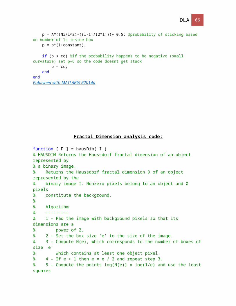
DLA 66
end %vline (subfunction)
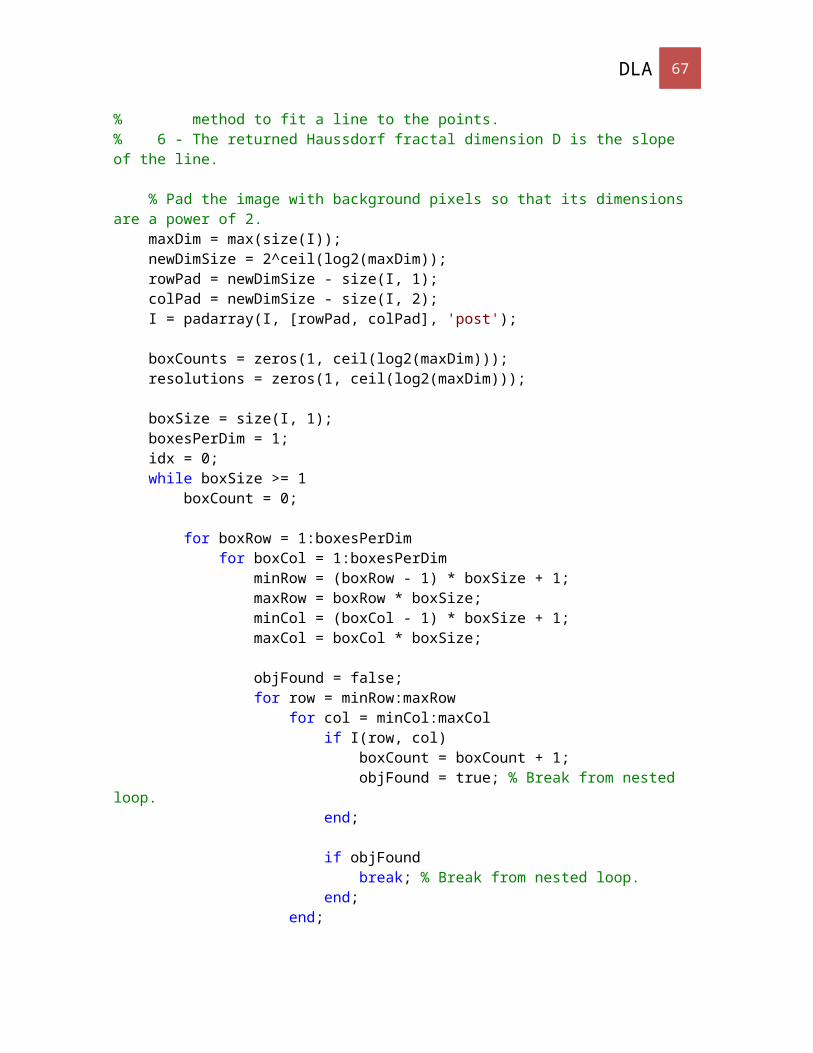
DLA 67
Works Cited
1. Daccord, Gerard, Johann Nittmann, and H. E. Stanley. "Radial Viscous Fingers and
Diffusion-Limited Aggregation: Fractal Dimension and Growth Sites." Physical Review
Letters 56.4 (1986): 336-41. Web.
2. Kadanoff, Leo P. "Simulating Hydrodynamics: A Pedestrian Model." Journal of
Statistical Physics 39.3 (1985): 267-83. Web.
3. Kondic, Ljubinko, Michael Shelley, and Peter Palffy-Muhoray. "Non-Newtonian Hele-
Shaw Flow and the Saffman-Taylor Instability." Physical Review Letters 80.7 (1998):
1433-436. Feb. 1998. Web. Mar.-Apr. 2015.
4. Kondic, Ljubinko, Peter Palffy-Muhoray, and Michael J. Shelley. "Models of Non-
Newtonian Hele-Shaw Flow." Physical Review E 54.5 (1996): R4536-4539. Nov. 1996.
Web. Mar.-Apr. 2015.
5. Mandelbrot, Benoit B. The Fractal Geometry of Nature. New York: Freeman, 1983.
Print.
6. Nittmann, Johann, Gerard Daccord, and H. E. Stanley. "When Are Viscous Fingers
Fractal?" Fractals in Physicals (1986): 193-201. Web.
7. Vicsek, Tamas. "Pattern Formation in Diffusion-Limited Aggregation." Physical Review
Letters 53.24 (1984): 2281-284. Web.
8. Witten, T. A., and L. M. Sander. "Diffusion-limited Aggregation." Physical Review
B 27.9 (1983): 5686-697. Web.