Embed Size (px)
Citation preview

dk Fermi National Accelerator Laboratory
FERMILAB-Pub-86139-T
April, 1986
CALCULATING HEAVY QUARK DISTRIBUTIONS
John c. conii Department of Physics, Illinois Institute of Technology,
Chicago, Illinois 60616, U.S.A. and
High Energy Physics Division Argonne National Laboratory
Argonne, Illinois 60439, U.S.A.
Wu-Ki Tung Department of Physics, Illinois Institute of Technology,
Chicago, Illi& 60616, U.S.A. and
Fermi National Accelerator Laboratory Batavia, Illiiois 60510, U.S.A.
A systematic calculation of the evolution of parton distribution functions including the effects of heavy quark mass~les is presented. The method involves the use of a special renormalization scheme which ensures ordinary massless evolution with the correct number of active quark tlavon at all stages, and specifies appropriate matching conditions at thresholds. This method is applicable to all orders of the perturbation expansion in principle, and it is simple to implement in practice. Results of this calculation using born distributions at low energies as input are examined and compared with published results. The heavy quark distribution functions are found to be about a factor of two larger then the well-known EHLQ results.
1. INTRODUCTION
Most interesting high energy processes shxiied at current accelerators as well as those pro-
jected for the future are described in terms of fundamental parton-parton (including gauge boson)
interactions. As the consequence of ‘factorization theorems, ’ l the cross-section for such a process
4s Operated by Universitler Research Association Inc. under contract with the United States Department of Energy
can typically be written as a sum of couvolution intcgmls. each consisting of a .bard xatteriux.
cross-section for elementary partons and a product of parton distribution functions ior the physical
hadrons. Thus reliable determination of the parton distribut.ion functions is a key element in the
study of all current and future high energy processes.
Published parameterizations of parton distribution functions are usually determined by fitting
xome set of data. Typically the data consists of structure functions from deep inelastic lepton
scattering, sometimes supplemented by cross-sections for Icpton-pair production in hadron-hadron
collisions. The lit is made to a set of QCD-motivated parametric functions which approximate the
required Qz-evolution in some mergy range. (Here Q is the scaie of the bard scatterinK. A typical
range of the kinematic variables covered in these fits is 0.05 < z < 0.8. 1.5 GeV < Q < 15 GeV).
Most work on the evolution of parton distribution functions applies the simple Altarclli-Parisi
equation with 3 or 4 massless quark flavon, and hence leaves out the direct and indirect effects of
the maples of heavy quarks. P&on distribution functions derived this way are clearly suspect for
use in the large Q domain (say of the order of the W- and Z-mass and beyond).
Not only are the distributions of the heavy quarks omitted, but the distributions of the light
quarks and of the gluon are affected by the neglect of the bcavy quarks. The effect is most
important in the small z region, where all the parton distributions (especially the gluon distribution)
accumulate at high energies. Reliable values of the parton distribution functions at small x are,
however, precisely what is needed in the calculation of most high energy processes in hadron
colliders?.
In this paper we describe a concrete calculation of the evolution of parton distributions using
the systematic methods of Refs. 3,4,5 to include the effects of heavy quark maaes. This method
employs a special renormalization scheme whose important property is that all subtractiona are
done either by minimal subtraction or at zero momentum with massless propagators. It therefore
has the distinctive advantage that massless evolution is used at all stages, with matching conditions
2

at the thresholds. Xs a result. the rules of calculation of renormalization group cocfficicnts and
hard scattering cross-sections are well-dr&ned to all orders. and they xc simpif* to carry ant, iu
practice. Herein is the improvement over the theta-function and other methods that have typicaliy
been used in other work.‘,“,’
The calculations are performed by a computer program that was also designed t,o provide ac-
curate calculations at small values of z. It carries out the evolution of the parton distributions.
given any specified set of parton distribution functions at a chosen initial scale Q = Qo, and given
a specified value of LJ~D. We have used the program to calculate the parton distributions ob-
t,ained by using various starting distributions corresponding to commonly rued parameterization?
We compare the results both v&h each other and with the results of Eichten et aL2 Above the
thresholds, our c&uIation yields considerably more heavy quarks than the calculation of Eichten
et al
in Sect. 2 we describe the renormalization procedure for crossing B quark flavor threshold. In
Sect. 3. we enumerate the QCD parameters which enter the calculation. We discuss in some detail
the definition of the running coupling o.(p) and the relationa between various definitions of &IJ
Sect. 4 spells out the numerical evolution procedure and Sect. 5 describes the main results of our
study. Sect. 6 contains summary remarks and discussion
2. Parton Evolution Across a Mass Threshold
In quantum field theory, parton distribution functions correspond’ to certain specialized
Green‘s functions. (Alternatively, moments of these functions correspond to hadronic matrix el-
ements of the twist-two operators of the theory.9) It follows that the precise definition of these
distribution functions must depend on the renormalization scheme adopted. The physical .&ucture
functiona for various experimentally measurable quantities are, of course, renormalization-scheme
3

independent. They are convolutions of parton diatributionfunctionr with hard acntlering ampiitudca
(corresponding to Wilson coefficients in the ianguage of the operator product expansion). Henrr.
the hard scattering amplitudes are also renormalization scheme dependent. and this dependeucc
compensates that of the parton distribution functions.
The methods of perturbative QCD are most simply applied either far below mass thresholds
(when the decoupling theorem ” ran be invoked) or far above thresholds (when the quarks can be
treated as massless). Our methods provide a systemat,ic way of working in threshold regions a4
well. The methods apply whatever the number of heavy quarks and irrespective of whether their
masses are close or far apart. Ry a heavy quark. we mean one whose renormalized maw parameter
is sufEciently larger than A. The charmed quark is presumably marginally heavy enough.
For the sake of clarity, let us focrls on one single flavor threshold, associated with a quark of
mass Mm+,. where n is the number of quarks with maSs less t,han M,+,. To define a perturbation
expansion in terms of renormalized quantities, we must introduce a scale parameter P. We let a.(a)
be the effective strong coupling at that scale. In a perturbative calculation of a hard-scattering
cross-section on an energy scale Q, /, must be chosrn to be of order Q.
Our parton distributions when calculated at a scale /J must rrflect the actual physics on scalrs
of order p. In particular, they must reflect the way in which the heavy quark appean. NOW. the
decoupling theorem tells us that when p < Mn+I, the effective number of flavors, net,, is n. On
the other hand, when p > M,+, , we should neglect the mass of the quark, so that nc,/ = n + 1:
the (n + l)th quark participates as fully in a hard scattering on such a scale as the lighter quarks.
Since the value of p does not correspond to exactly one particular value of a momentum, it
is not possible to find a precise value of /1 that correspond4 to the quark threshold. Rather we
will choose a threshold value p = pn+L by the natural convention that the effective coupling is
continuous. We will see below that in our scheme, with m renormalization for light quarks, this
threshold value is p,,+, = Ma+, Above this value. we define nc,, = n+ 1. while below it we defme
4

“c,, = n.
The renormaiization scheme we choose to we was first &lined by Collins. Vilczek. ad Zer.“.’
It applies the m prescription to Feynman diagrams without amy heavy quark lineu. ad zero-
momentum subtraction (BPHZ) otherwise. For t,his pwpose. n quark is treated as ireavy or light
according to whether p is greater or less than the associated threshold. as defined above. Thus
if the only relevant heavy quark is the one of mass Mnti, then the scheme amounts to witchiiq
between two schemes. R” and R’.
The scheme R” is rxactly the same as hhe osuai MS srheme: it is an appropriate xhrmc
when or > Mm+,. The formulas for the coupling I., Wilson roefficirnrs <and rmormniizatioo
group coefficients (including the Altarelli-Parisi evolution kern&) are ail st,andard. The number
of flavors which appears in these formulas is (n + 1). These results cannot be extended into the
p < M,+I region because the perturbation series contain terms such as [a.(/~) In(M,,+,/~)lt, so
that the higher-order terms would not be smaller than the lower-order terms.
In the R’ scheme, we only apply m subtractions to those graphs that have no heavy quark
lines. (For the cake at hand M,+, is heavy.) Other graphs are subtracted at zero external momen-
tum. and with the light-quark masses set to zero. It can be demonstrated that this scheme does not
induce extra infrared divergences, and that it preserves gauge invariance.3-‘.‘1 For Green‘s func-
tions whose external momenta are much less than M,+, , the (n + 1)th quark flavor is decoupled.
This is manifest in this scheme: the effective low-energy theory, with n quarks. is obtained merely
by dropping all graphs that contain heavy quark lines, without needing to adjust the value of the
coupling. The formulas for the running coupling o,(p), th e renormalization group coe&ients. the
Altarelli-Parisi evolution kernels, etc are the nme as in the KG scheme when the number of flavors
is n. The R’ scheme is not very useful for Green’s functions with momenta far above the threshold.
since there are logarithms of the ratio oi momenta to the heavy mass.
The overall renormaiization scheme. denoted by R. consists of combining the ii!’ scheme above
5

threshold with the R’ scheme below threshold. The implementation of this method require3 the
calculation of the (finite) renormalization coefficients needed for t,he transition R” ++ R’. and the
specification of the threshold where this transition takes place.
Now to first order in a,, the relation between the couplings in the two schemes is5
af(/4)=o;(p) l--$Ll~ [ Ir2 I
It is convenient to choose the threshold p,,+l such that the transition R” ++ R’ results in a
continuous effective running coupling
64. when P > hn+~> Q!(P), when p < b+,
From eq. (I), it is clear that the appropriate choice is
The relation between the parton distribntions must have the form
/,‘(Z,P) = fl(z,a) + */,I $-p::‘59 ~)~h). I
(2)
(3)
(4)
where f;(z, JL) is the distribution function of pa-ton i at scale /1. The coefficients C! can be found
in Ref. SQ. When p is below A+,, the distribution function for the (n + I)th quark is suppressed
by a power of its mass, and we therefore neglect it. TIms, the only coefficients Ci in eq. (4) which
concern us are C; and CL, where p denotes the gluon and H the heavy quark. The other coefficients
are either higher order in a, or else multiply into p,, which vanishes at threshold. At our chosen
threshold, /~,,+l = &&+I, both C; and C& vanish, as they are proportional to lnM,,+l/~, just like
the first order term in eq. (1). It follows that all our parton distribution functions are continuous
at the t.hreshold given by eq. (3).
G

3. QCD Parametenr
The basic QCD parametera are: the total number of quark flavora nf, the rna~s parameten
of the quarks, M,,(n = 1,2, . . . . n,), and the coupling, a.. Now the value of the coupling (and also
of the masses) depends on the scale parameter, p, introduced in the renormalization procedure.
It is generally convenient to parameterize the dependence on /, by a single parameter A with the
dimensions of rnas~‘~. Since the value of A is scheme dependent and we have chosen a somewhat
unusual renormalization scheme, it is necessary to explain our definition of A, as well aa its relation
to the conventional values quoted in the literature.
The parameter A enters QCD calculations only through the running coupling a.(p). When
we have one or more heavy quarks in the theory, the effective number of quark flavors depends
on the renormalization scale p (which is usually chosen to be equal to the momentum scale Q of
the application). For A4,, < p < &+I, the effective number of flavors is defined to be n. Then
the effective value of A in this region. denoted by A(n), is related to a.(p) by the second order
formula’*
h(n) a*(p) = h$,A(,,)Z
1 _ b,(n)z Inlnp*/A(,@
> b(n) h~*/A(n)’ ’ (5)
where
b,(n) = 12.7
33-2n’
b(n) = 24*
153 - 19n
The values of A(n) for different n are not independent. The relation between adjacent ones,
A(n) and A(n + I), is determined by the relation (I) between the corresponding couplings. Thus.
only one of the nf numbers {A(n)} can be independently chosen. We make the convention that
A(nf) is the independent variable and denote it simply by A. This is the conventional Am in the
complete theory, with n, quarks.
7

Given A (= A(n,), we can obtain the values of A(n),n = n, - 1. “1 - 2, . . . . 1 numerically. by
solving eq. (1) at the threshold. Alternatively, we can expand the two sides of the equation in
inverse powera of In($/A(n + 1)‘) and take the lead&most powers. This results in:
In [A;‘$] = [l - b,$‘L)] h [A(t?+$]
- b,(?;;;n: I)] lnln [A(tt+i)2] (6)
+ [ii%] Ln [“‘i:,:,“] + cJ (Ln(M.:l,b(J Each time a,(p) is needed, we Grst determine n by the condition M, < p < A&+,, and then use
eq. (5) to evaluate the running coupling (to second order).
A detinition of A that is often used in phenomenological analyses of data is the “leading order’
(or ‘first-order”) ALO, which is related to a.(p) by the first term of eq. (5) with a fixed number of
quark flavors n (usually taken to be 3 or 4).
This definition is simple but incorrect in principle. In particular, from the calculable correction
terms, it is known that ALO measured in different processes or at different energies will - in
value, although a properly defined A should be a constant in QCD. Furthermore, even in work
where the full formula eq. (5) is used, the number of quark flavors is often taken to be a constant
(typically 4).
It is useful to establish a correspondence between our A-parameter and the A-parameters used
in standard analyses, by requiring approximate equality between the functions o.(p) in the schemes
over a limited range of p. (It is not possible to enforce agreement for all p’*.) We choose this range
to be around /? - 10 GeV’. Since a.(p) only varies 81owIy, the res&s are not very sensitive to
this choice.
In fig. 1 we plot, aa functions of our A, the equivalent values of ALO and of Am with the usual
choice n = 4 for these last two values. For our prescription, we have set n, = 6 and have chosen
{M;. i = 1, .._, 6) to be equal to their conventional values. (We have assumed M, = 40 GeV.)
8

In iig. 2 we plot a.(p) as a function of p over the range 1.5 GeV < fi < 10’ CeV for the
three schemes described above. For the two schemes with fixed flavor number. we have set this
number to four. We choose ALO = 0.2 GeV and set the A-parameters for the other schemes to their
corresponding values determined from fig. 1. The graph is divided into two ranges of p in order
to show the details of the comparison. Since the function a.(p) for a fixed number of (massless)
quarks haa monotonic and continuous derivatives, the fir&-order and m curves cross only at one
point. On the other hand, our a.(p) feels the effect of the heavy quark thresholds. The function is
required to be continuous at the thresholds: but its first derivative changes its value going through
each threshold, reflecting the turning-on of the new flavor degree of freedom. This can be seen in
fig. 2 by the fact that our a.(p) curve oscillates around the first-order a,(p) curve aa we pass the
successive thresholds.
It is of obvious interest to compare our results with the widely used parameterieation given
by EHLQ’. So let us note the pertinent features of their procedure for treating heavy quark
masses. They choose the threshold, h in p for each heavy quark to be /our timea the quark’s mws
parameter. At the same time a.(p) is calculated by the lowest order formula and is required to
be continuous at P = IL.. The consistency of these choices appears to be questionable; however,
in practice. the two curves for a.(r) can be made very close, provided the value of A is adjusted
appropriately. If we plot a.(~) based on the EHLQ formula on Figs. 2 a,b, it will interpolate
between the first order II, (dashed curve) at low /I and our full formula (solid line). But the value
of A that will do this ia not the same as any of ours.
4. CALCULATIONS
We appiy the renormalization procedure describing in the previous two sections to the renor-
9

malization group equations obeyed by the parton distribution functions (Altareiii-Parisi equation):‘3j
p~f~(z,p) = y ’ du i C’ .Jj s+.bl’f$,Pi~ (7)
where i, j are parton labels, and {I’!} are renormalization group coefficients (‘evolution’ kernel
functions). The functions {P:} in our scheme coincide with the standard expressions” in the m
scheme, when the number of quark flavors is set to the effective number of flavors nefl at the scale
p. We solve these integro-differential equations numerically, starting from an initial value JL = Qiai
and evolving through successive thresholds to obtain the full set of {/i(z,p)} over the desired
range of z and ~1. At each of the intermediate thresholds. the parton distribution are continuous.
for reasons discussed in Sect. 2, but the evolution kernels change due to the opening up of the new
quark-flavor channel.
Since existing parton distribution function parameterizations appear to give an adequate repre-
sentation of experimental deep-inelastic structure functions in the currently available energy range,
ve do not make any attempt to fit data with our calculations. Our emphasis is on studying the ef-
fects of the opening of heavy quark flavor channels on the evolution of parton distribution functions
from current energies to those of interest in future accelerators. To this end. we use standard pa-
rameterizations of the parton distributions to provide the input set of parton distribution functions
at p = Qini , and then generate the full set of parton distribution functions over the desired range.
We then examine the heavy-quark distributions at high energies. We also compare our results with
some existing estimates of heavy quark distributions, and compare results obtained with different
sets of input with each other.
In solving eq. (7), we tint separate the (flavor) singlet and non-singlet parts of the quark
distribution functions. Let i = 1,2, ___, G denote the quark flavors, i = -I..., -6 the corresponding
anti-quarks, and i = 0 the gluon. Then we define the singlet-quark distribution function as
fS(Z? Pi = OK++’ + f-42, P)l. (8) I>0
10

The non-singlet part of each Eavor distribution function is then debed as
where n,fl(p) is the number of active quark fIavon, at scale p.
The singlet quark function fS and the gluon function f;=o satisfy a set of (two) coupled
equations. Each of the non-singlet function /,y” evolves independently by itself. Hence. the initial
functions f;(z,p = Qid) are split into singlet and non-singlet pieces according to eqs. (8) and (9);
the evolution in p is then performed for {fs, fo} and {fy’}. Fimily we reassemble the results to
obtain the full fi(z,p) for the desired range of z and b. We do not employ the usual separation
of parton distribution functions in terms of ‘valence’ and ‘sea’ distributions. Each of such schemes
presumes certain symmetries of the ‘sea’ distributions which are not necessarily n consequence of
QCD, and are subject to modifications in the light of improved experimental data.
5. RESULTS
Much recent work on high energy processes involving heavy quarks has used the parton dis-
tributions calculated by Eichten et aL2 It is therefore of interest to calculate parton distribution
functions in our renormalization scheme using the same input QCD parameters and initial distri-
butions as EHLQ, and to compare the results at high energies.
In general. we obtain heavy quark distribution functions that are substantially larger than the
corresponding ones obtained by EHLQ. For a first look, let us check the second moment of the
distribution function. It measures the momentum fraction carried by the parton. In fig. 3a we
show the second moments of the ‘sea-distributions’ (u, d, s, c, b, and t) from Set 1 of EHLQ as
functions of Q in the range 2.5 GeV < Q < 10’ GeV. To compare with these results, we plot
in fig. 3b these same moments obtained from our distribution functions computed with the same
input distributions at f&pi = 2.5 GeV and equivalent QCD parameters to those of EHLQ.
11

The moment of the distribution of a heavy quark (c, b, or t), as given by our calculations.
evolve at a similar rate in LnQ to that for a light quark (u, d. or a), once we are much above the
threshold for the heavy quark. On the other hand, the EHLQ moments show two distinct rates
of evolution, with the heavy flavors clearly growing more slowly. As a consequence, we obtain
substantially more heavy quarks than EHLQ. The ratios of corresponding (heavy quark) moments
from the two sets lie in the range 1.C to 2.0 from Q = 10’ GeV down to a few times the threshold
value for each flavor. The light sea-quark moments behave qualitatively similar for the two sets,
with our results somewhat lower than those of EHLQ. The II-, d- and gluon- moments are plotted
against In Q for the EHLQ distributions (dashed lies) alongside those from our distributions (solid
lines) in fig. 4. We we that the gluon momentum fractions have somewhat different evolution in
the intermediate energy range, and that our gluon fraction is smaller (reflecting more ‘leakage’ to
heavy quark flavors). The behavior of the u- and d- moments are similar in the two e&s, with our
results again being slightly smaller than the other set.
The trends indicated by the momentum fraction manifest themselves in other ways. In fig. 5
we present {h(z, Q)} aa functions of In Q in the same range as above, with z 6xed at IO-‘, a typical
value of interest at the next generation of accelerators.* Fig. 5a shows the sea distributions of EHLQ
set 1; and fig. 5b shows the corresponding curves of our calculation. The distinctive slower rate
of growth for heavy flavors in the EHLQ set is again apparent. This feature is more pronounced
at smaller z, e.g. z = 10m4, and less 80 at higher values of z. In fig. 6 we plot the distribution
functions Venus z in the range IO-’ < z < 5 x 10m2 for a f?xed value of Q = 83 GeV. Fig. 6a shows
the gluon-, u-, and d- curves from EHLQ set 1 and from our work. All three distributions from the
two sets behave similarly. Fig. 6b shows the u-, d-, s-. and c- distributions; and fig. Gc the b- and
t- distributions. We see that the difference in the size of corresponding heavy quark distributions
from the two sets (by about a factor of 2) is relatively uniform in this z range.
It should be noted that EHLQ adopt mass-dependent evolution kernels, following the prescrip-
12

tion oi Gliick. Hoffmann and Reyai5. The differences produced by t,he modified kemeis are insigniii-
rant except near the thresholds. Furthermore. these differences c~1. in principle. he compensated by
differences in the hard-scattering cross-sections, ii both schemes are applied self-consistently. The
prescription for calculating hard-scattering cross-sections appropriate to matching the prescription
for EHLQ’s parton distributions has not been explicitly discussed. to our knowiedge.
However, we do not believe that the di&rences in the heavy quark distribution functions
between the EHLQ set and OUA can be explained by differences in the choice of threshold points
and other detailed prescriptions near the thresholds. The reason is that far above the thresholds. the
logarithmic derivative of the sea distribution functions and of their moments should be dominated
by the gluon term. Thus they should be Ravor-independent. This feature is independent of the
prescriptions adopted near the thresholda. The logarithmic derivatives can he read off figs. 3,-S
simply aa the slopes of the curves. It is manifest that our distributions have flavor independent
SlOp?S.
We can also investigate the question: How much do our results on the partook distributions.
especially for the heavy quarks. depend on the input distributions? The answer can he obtained
by comparing results derived from different sets of inputs all of which fit low energy data. In
particular, we have systematically compared results derived from input functions of EHLQ set 2
nnd of the Duke-Owen@’ set 1, in addition to EHLQ set I as presented above. The predicted heavy
quark momentum fractions are almost the same in all three cases. This is perfectly understandable
as heavy quark evolution is driven mostly by the gluon distribution; the gluon momentum fraction
is similar in all sets of partan distribution functions.
We show in fig. 7 the momentum fraction carried by the sea distributions, u, d, s, c, h, and
t as functions of InQ in the same range as before. The curves of fig. ‘la are calculated using the
Duke-Owens parameterization: those of fig. 7b are our rcsuits ruing the Duke-Owens distributions
at Q = 2.5 GeV as input. The v&e of A used in the caiculation corresponds to that of Duke-
13

Owens in the sense described in sect. 3. We note that: (i) the c-, h-, and t- curves are almost
indistinguishable from the corresponding ones in fig. 3b; (ii) Duke-Owens uses a SU(3)-symmetric
sea, hence the u-, d-, and s-curves coalesce into one; (iii) there are no heavy quark lines in fig. 7a
since the Duke-Owens parameterization assumes four (6xed) flavors; and (iv) the abnormal behavior
of the two curves in fig. ‘la above Q N 800 GeV reveals the upper limit of the range of applicability
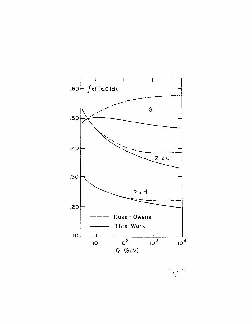
of this parameterization (note the change of scale in the ordinate). For completeness, we show, in
fig. 8, the momentum fraction carried by the gluon and the u- and d- quarks. Our curves (solid
lines), especially the gluon one, are consistently lower than those of Duke-Owens (dashed lines) due
to the creation of the heavy quark fiavors. In contrast to the second moment. the z-dependence
of the distribution functions for the various flavors and the gluon from the various sets can differ.
The difference diminishes, however, as Q increases.
6. DISCUSSION
We have men that the evolution of pm-ton distribution functions in p, incorporating quark flavor
threshold effects, can be formulated in a systematic way utilizing an appropriate renormalization
scheme. The scheme adopted here is the natural extension of the conventional m echeme, giving
the appropriate number of active quark flavors for any given scale F. In applying the parton
distribution functions calculated in this scheme to physical processes, it is necessary to fold in the
relevant hard scattering cross-sections (or Wilson coefficients) defined in the same scheme.
Most phenomenological applications in the literature use the leading order expressions for the
hard scattering amplitude and ignore quark masses. This is not a good approximation when large
coefficients in the first order QCD correction term are known to exist (e.g. z*.terms in lepton-pair
production), or when the relevant physical variable Q is not far above some heavy quark threshold.
Under the latter circumstance, inclusion of mass effects in the hard scattering amplitude is clearly
14

3ecded to properly account for the smooth turn&-on of a new thrcshoid for we spcciSc process.
Paying attention to both types of correction miil en.wre 3 more meaningi% comparison of theory
with experiments. Failure to do 80 can lead to misieading discrepancicv in fitted vaiues of QCD
parameters or in features of the parton distribution iunctions.
The heavy quark distribution functions in nucleons, derived from our calculations are roughly
a factor of 2 bigger then those obtained by EMLQ. RI ore heavy quarks (at smail z) will enhance
processes which are dominated by incoming heavy quarks. A typical case is Hiqgs production in
a mass raqe where it is made by quark annihilation. (Its coupiing to a qurk is proportionai to
the quark’s mass.) Even with our disttihution functions, however, the heavy quark flavor content
of the nucleon is still quite small compared to the values for gluons and valence quarks.
We have Seen that the method of generating parton distribution functions by direct numerical
solution of the evolution equations works easily for any chosen set of values of input distribution
functions and fundamental QCD parameters. They satisfy the QCD renormalization group equa-
tions and incorporate heavy flavor thresholds. This method provides a more Eexi’ole and more
powerful alternative to the nx of fixed parameterizations of the parton distributions in B wide
variety of applications to high energy processes.
The programs for these calculations are integrated into a package which also con&u (a)
routines which evaluate the widely used parameterizations for parton distribution functions, and
(h) an interactive module which allows the convenient comparison of various parton distribution
functions as functions of z and F, and of moments of parton distribution functions aa functions of
/A. The subprogram to solve the evolution equations contains parameters which control the desired
accuracy of the numerical calculations. For any given set of QCD parameters and input functions.
the calculation to generate the full set of {f;(z,p = Q)} for 10m4 < z < I and 2 GeV < Q <
IO’ GeV with less than 2 - 3% error takes a few minutes of CPU time on a VAX 780. (This
-rogram is available to interested users upon rrqwst.)
15

This work was supported in part hy the U.S. Department of Energy under contract DE-
FG02-85ER-40235 and hy the National Science Foundation under grant numbera PHY-82-17352
and PHY-85-07635. JCC would like to thank the Institute for Advanced Study at Princeton for
hospitality while part of this work was performed.
REFERENCES
[l] D. Am& R. Petmnzio, and G. Veneziano, Nucl. Phys. j&&j, 29 (1978); S.B. Libby and G. Sterman. Phys. Rev. m, 3252 (1978); A.H. Mueller, Phys. Rev. m, 3705 (1978); S. Gupta and AX. Mueller, Phys. Rev. m, 118 (1979); R.K. Ellis. H. Georgi, M. Machacek, H.D. Politzer and G.G. Ross, Nucl. Phys. Jj$& 285 (1979); J.C. Collins and G. Sterman. Nucl. Phys. j$l&, 172 (1981).
[2] E. Eichten, 1. Hiichliffe, K. Lane and C. Quigg, Rev. Mod. Phys. a, 579 (1984). [3] J.C. Collins, F. Wilczek and A. Zee, Phys. Rev. m, 242 (1978). [4] J.C. Collins, ‘Renormalization’, (Cambridge University Press, Cambridge, 1984). [S] S. Qian, Argonne preprint, ANGHEP-PR-84-72, and ‘I? 7 ‘Theis’s ( j98.7) [S] Y. Kacama and Y.P. Yao, Phys. Rev, m, 1605 (1982); W. Wentzel, Nucl. Phys. m, 259
(1982). [7] E.g., D.A. Ross, Nml. Phys. m, 1 (1978). [8] J.C. Collins and D.E. Soper), Nucl. Phys. u, 445 (1982). [9] D. Gross in ‘Methods in Field Theory’, R. B&an and J. Zinn-Justin (eds.) (North-Holland,
Amsterdam, 1976). [lo] T. Appelquist and J. Camezone. Phys. Rev. m, 2856 (1975); K. Symanzik, Common. Math.
Phys. a, 7 (1973); E. Witten, Nucl. Phys. m, 445 (1976. [ll] Kazama and Yao in Ref. 6. 1121 W. Bardeen et al., Phys. Rev. m, 3998 (1978). (131 V.N. Gribov and L.N. Lipatov, Sov. J. Nucl. Phys. s, 438, C75 (1972); Yu.L. Doksbitzer,
Sov. Phys. JETP 44, 641 (1977); G. Altarelli, and G. Parisi, Nucl. Phys. ElZ.& 298 (1977); P.W. Johnson and W.-K. Tung, Phys. Rev. m, 2769 (1977).
[14] W. Furmanski and R. Petronzio, Z. Phys. m, 293 (1982). [15] M. Gliick, E. Hoffmann and E. Reya, Z. Phys. m, 119 (1982). 1161 D. Duke and J.F. Owens, Phys, Rev. m, 49 (1984).
FIGURE CAPTIONS
Fig. 1 Equivalent values of Am and A ~0 (for 4 massless quark tlavors) as functions of A (the QCD
SC& parameter appropriate for 6 flavors with physical mass thresholds). Corresponding A’8
yield comparable a.(p) in the range 2 GeV < Q < 5 GeV when used in their respective
contexts
16

Fig. 2 The ruming coupling aa a function of p for three definitions of a.(p) : (i) the solid line
represents eq. (S), using 6 quark fiavors with decoupling taken into account at lower energies;
(ii) the dashed line represents the ‘i%st order’ o.(r) using 4 flavors: and (iii) the dotted line
corresponds to the second order QCD a.(p) evaluated in the MS scheme with (fixed) 4 flavors.
The A-v&m used are those corresponding to ALo = 0.2 GeV (fig. 1). The two parts of the
figures shows two separate ranges of p.
Fig. 3 Second moments of the ‘ma distributions’ as functions of In Q. Part (a) is for EHLQ distribution
functions; part (b) shows the same moments obtained from our calculation.
Fig. 4 Same as fig. 3 for the valence quarks and glum. EHLQ results are in dashed lines; our results
in solid lines.
Fig. 5 Parton Distribution Functions at f&d z = IO-’ plotted against IogQ: EHLQ results (dashed
lines) in part (a) and our results (solid lines) in part (b).
Fig. 6 Logarithm of Parton Distribution Functions at fixed Q = 83 GeV plotted against log%. Keys
to the curves are given on the graphs. Part ( ) h B 8 ows the glum and the valence quarks; part
(b) shows the lighter sea-quarks u, d, s, and c; part ( ) h c J ows the heavy quarks b and t.
Fig. 7 Second moments of sea-quark distributions from Duke-Owens parameterization set I (part a)
compared with our results (obtained with Duke-Owens input) (part b). Except for the break
in the vertical scale in part (a), these plots can be directly compared with fig. 3.
Fig. 8 Some M fig. 7 for the glum and the valence quarks. (cf., fig. 4).
I7

0.7
0.6
0.5
0.4 > $
0.3
0.2
0.1
C ,L 0
I I I I I
/
A (GeV)

1 I I I I I 1 1.5 2 3 5 7.5 IO
p
(G:“)
.06 I I
--- FIRST ORDER
THIS PAPER . . MS (Mi = 0)
IO' IO' p (GeV)

e 9 0 O.?
;: 3
-25 .+.
< I
\ \ 1 I ’ \
I \’ ’ \ \ \ \ ’ ‘\ \‘\Z \ \ y
\ \+\w- \ \ \ \ a\ \ ’ ‘1 ’ \ I-0 \ ‘\ ‘,
\ \ \ \ \ \
a I3 \
\ \
v, \ x
\ ‘1
\ \
\
w- \
\ \ ‘,-
I \ \
4
,
\
\,
\
“0
? 0 -
2
“0 52 -
0
-0
0

.60
.50
.4c
.3c
.2(
.I(
‘/ xf (x,o)dx
I ----v-
--- EHLQ
This Work
I I I
I I I
IO' IO2 IO3 IO4
Q (GeV)

I
‘\ \\ v IU ’ I
‘\ \ ‘\ ’ v \\\+ CJ v. \ i! .^
c
‘0 - i; I, x’ x
\,\., \ fi 4-i > ‘:\ \ - \\ ‘\
,’ Y2 \‘. -\\‘\ \ ~\\ ‘A 1
tL& c x
I I 0 0 u-l u-l oi oi
0 0 2 2
‘\\ ‘1 ‘\I \ I- \\ \ 2 ---I-l ‘3
In 0 d

50
40
30
20
IO
5
4
3
2
I
\ \
Q=83GeV
EHLQ This Work -- . . ..a -se U
x5 ----- --- d
10-4 10-3 10-Z X

0 In* Fl RI - Ei ti dd d d 6 d
I IIll 1 I I I I I ./ ’
0 In* Fl RI - Ei ti dd d d 6 d
IIll 1 I I I I I ./ ’ ./
.A ,(I
c3 /$jp-
/’ :. . .
_
II ./@-’ /,’ .:; /”
0 .//’
KY/, .(A.$ “.
. . .* &;,/
,;+y . .:- ,/B/’ / 2.
%- /T ‘. ’ \+
/;’ , ,’ . I I
III1 I I I I 1 . :Y/ ’ .z< /,A
Y 0 -
i) \i,
X q ri
: 0 -
c ‘0 -
./;;;2- / 2 u :
, ..2p ,/’ . ..g/
Y. / II .&’
u Jg’ ,’ / *ljI -
1 ,I
:g! 1 X
V’ //
0
- 2 /‘;< 0 . ‘0 -I : f I
5,,/ ,’ 1. I w: 1 I -
A, I I
.tiv / I-0 Iv) IV
1.z <I 1 ; vi 6 *
I I I I I . ‘0 0 10-3 0 N In -
dd d 6 0 d

I---- l I I
5, I I ‘* I $
\ /
‘\ \ 2 1-0 \ \* 2 1; \ ‘. nl A \ \ \ \ ;: \ G \ \ . -5 \ \
< l >%J \ \ -0
\ \ \ \ I \ \
;: m 9 5,
0
IO' IO2 IO3 IO4 Q (GeV)
![Cement and Concrete Researchdownload.xuebalib.com/xuebalib.com.18512.pdf · of the pore system, fly ash based GPC can passivate the reinforcement steel as efficiently as PCC [24–28]](https://img.pdfslide.us/doc/110x75/6063c27f36a6ff76995a685d/cement-and-concrete-of-the-pore-system-iy-ash-based-gpc-can-passivate-the-reinforcement.jpg)