Django-Jorek code: a numerical box for MHD discretization

Django-Jorek code: a numerical box for MHDdiscretization and JOREK

A. Ratnani2,B. Nkonga35, E. Franck1,C. Caldini-Queiros2,L. Mendoza2, G. Latu4, V. Grandgirard4, E. Sonnendrucker26,

M. Holzl2, H. Guillard 5

, ,16 September 2015

1INRIA Nancy Grand-Est and IRMA Strasbourg, TONUS team, France2Max-Planck-Institut fur Plasmaphysik, Garching, Germany3Nice university, Nice, France4CEA/DSM/IRFM, Cadarache, France5INRIA Sophia-Antipolis, CASTOR team, France6TUM center of mathematics, Garching, Germany

E. Franck Adaptive Preconditioning 1/20

1/20

Outline

Context and the Django code

Model in Django DJANGO

Spatial discretization and meshes in DJANGO

Preconditioning and solver in DJANGO


2/20

Context and the Django code


3/20

Physical context : MHD and ELM’s� In the tokamak plasma instabilities can appear.

� The simulation of these instabilities is an importantsubject for ITER.

� Examples of Instabilities in the tokamak :

� Disruptions: Violent instabilities which can seriouslydamage the tokamak.

� Edge Localized Modes (ELM’s): Periodic edgeinstabilities which can damage wall components dueto their extremely high energy transfer rate.

� These instabilities are described by MHD models like

∂tρ +∇ · (ρu) = 0

ρ∂tu + ρu · ∇u +∇p = J×B−∇ ·Π

1

γ− 1∂tp +

1

γ− 1u · ∇p +

γ

γ− 1p∇ · u +∇ · q

= 1γ−1

mieρ J ·

(∇pe − γpe

∇ρρ

)−Π : ∇u + η|J|2

∂tB = −∇×(−u×B + ηJ−mi

ρe∇pe +

mi

ρe(J×B)

)µ0∇×B = J, ∇ ·B = 0

� ELM’s Simulation


4/20

Aim and principle of DJANGO project

Aim of DJANGO project� Develop a library to test and validate the numerical methods which we use in the

MHD codes with

� more simple models,� more simple geometries and meshes,� more simple cases.

� Validate the future numerical heart for JOREK 3.0

Numerical heart of DJANGO� Full and reduced MHD with bi-fluids and diamagnetic terms.

� Arbitrary high-order and stable Splines on quadrangular and triangular meshes usingBernstein formalism with refinement.

� New toroidal basis or flexible toroidal discretization.

� Adaptive preconditioning and Jacobian-free method.

� Possible coupling with kinetic codes like Selalib.


5/20

Models in DJANGO


6/20

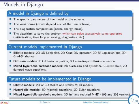
Models in Django

A model in Django is defined by� The specific parameters of the model or the scheme.

� The weak forms (which depend also of the time scheme).

� The diagnostics computation (norm, energy, mass).

� The algorithm to solve the problem which can solve successively some operators(initialization, time loop or solving, diagnostics, etc).

Current models implemented in Django� Elliptic models: 2D-3D Laplacian, 2D Grad-Div operator, 2D Bi-Laplacian and 2D

Grad-Shafranov

� Diffusion models: 2D diffusion equation, 3D anisotropic diffusion equation.

� Mixed hyperbolic-parabolic models: 2D Cartesian and cylindrical Current Hole, 2Ddamped wave equations.

Future models to be implemented in Django� Elliptic models: 2D or 3D stokes and stokes-MHD models.

� Hyperbolic models: 3D Maxwell equations, 2D Euler equations.

� Mixed hyperbolic-parabolic models: 3D full and reduced MHD (199 and 303 version).


7/20

Spatial discretization and meshes in DJANGO


8/20

Meshes and discretization in DJANGO

3D geometry� Currently the code allows to use 3D geometries: cylinder or torus.

� Current strategy: Tensor product between 2D poloidal meshes and 1D toroidaluniform meshes.

� Future strategies: Tensor product or real 3D triangular or quadrangular meshes.

2D poloidal Meshes� Triangular or quadrangular meshes generated by CAID (code of A. Ratnani) based on

isoparametric and isogeometric approach.

Remarks� Currently the poloidal and toroidal discretization are separated.

� future works and researches: would be realized on the non-singular meshes in theisoparametric or isogeometric context.


9/20

Current discretization in DJANGO

Philosophy of the discretization� Isoparametric and isogeometric approachs: the physical function are represented with

the same basis functions of used to represent the geometry.

� These approaches allow to align and adapt the meshes to the physical flows (surfacesaligned mesh).

Current discretization in Django� Hermite Bezier finite element basis (used in JOREK) with different quadrature rules

implemented.

� B-Splines finite element basis with arbitrary order (1 to 5 actually) and regularity (C0

to Cp−1).

� Remark: the B-Splines on triangles and quadrangles are unified using Bernsteinformalism (A. Ratnani)

� Box-Splines finite element: Splines with quasi-interpolation on triangle used also inSelalib for transport problems on Hexagonal meshes (L. Mendoza).


10/20

Results for B-Splines and Bezier elements in DJANGO� Convergence of poloidal discretizations.

Cells2D laplacian 2D Bi-Laplacian 2D-WaveErr Order Err Order Err Order

HBezier

16*16 2.9E-5 - 3.4E-5 - 2.8E-5 -32*32 1.9E-6 3.9 2.1E-6 4.0 1.8E-6 3.9564*64 1.2E-7 4.0 1.6E-7 3.8 1.2E-7 3.9

B-S2 c0

16*16 - - - - - -32*32 - - - - - -64*64 - - - - - -

B-S2 c1

16*16 - - - - - -32*32 - - - - - -64*64 - - - - - -

B-S5 c0

16*16 - - - - - -32*32 - - - - - -64*64 - - - - - -

B-S5 c4

16*16 - - - - - -32*32 - - - - - -64*64 - - - - - -

� Efficiency and conditioning of poloidal basis (Mesh 64*64).

Nb dof time solvingC0 Cp−1 C0 Cp−1

BS p=3 36481 4225 - -BS p=4 65205 4356 - -Hezier 16384 - 4.4E-3 -


11/20

Future poloidal discretization in DJANGO

Aim:� Arbitrary high-order and stable Splines on quadrangular and triangular mesh using

the Bernstein formalism with refinement.

Future works with new PhD student:� B-Splines on quadrangular and triangular mesh using Bernstein formalism (A.

Ratnani)

� Refinement of the mesh, order and regularity for B-Splines (A. Ratnani, E. Franck +PhD) also to construct low-order and adaptive preconditioning (next section).

� Compatible finite element using the DeRham sequence to obtain a stablediscretization for non-coercive problems or for problems with involutive constraints (A.Ratnani, E. Franck, E. Sonnendrucker + PhD).

� Theoretical study of the stability and convergence of these elements (A. Ratnani, E.Franck, E. Sonnendrucker + PhD).

Other works:� Stabilization for convective problems using Petrov-Galerkin methods (B. Nkonga).


12/20

Future and current toroidal discretization in DJANGO

Aim:� New toroidal basis or flexible toroidal discretization.

Current toroidal discretization in DJANGO:� 1D B-splines (the 3D basis is obtained by tensor product).

� Classical Fourier expansion.

Future toroidal discretization:� Two possibilities: find the more adapted basis (actually it is not clear) or propose

different toroidal discretizations and switch depending on the test case.

� Possible discretizations

� 3D B-Splines on triangular meshes.� 3D B-Splines on mixed triangular-quadrangular (aligned ?) meshes.� Fourier method. Classical Fourier method (current JOREK method) or Mapped

Fourier method (H. Guillard)


13/20

Preconditioning and solver in DJANGO


14/20

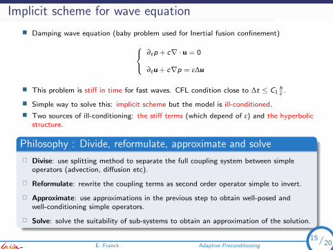
Implicit scheme for wave equation

� Damping wave equation (baby problem used for Inertial fusion confinement) ∂tp + c∇ · u = 0

∂tu + c∇p = ε∆u

� This problem is stiff in time for fast waves. CFL condition close to ∆t ≤ C1hc .

� Simple way to solve this: implicit scheme but the model is ill-conditioned.

� Two sources of ill-conditioning: the stiff terms (which depend of ε) and the hyperbolicstructure.

Philosophy : Divide, reformulate, approximate and solve

� Divise: use splitting method to separate the full coupling system between simpleoperators (advection, diffusion etc).

� Reformulate: rewrite the coupling terms as second order operator simple to invert.

� Approximate: use approximations in the previous step to obtain well-posed andwell-conditioning simple operators.

� Solve: solve the suitability of sub-systems to obtain an approximation of the solution.


15/20

Principle of the preconditioning� The implicit system is given by(

M UL D

)(pn+1

un+1

)=

(Rp

Ru

)

with M = Id , D =

(Id − cθε∆ 00 Id − cθε∆

), L =

(θc∆t∂xθc∆t∂y

)and U = Lt .

� The solution of the system is given by(pn+1

un+1

)=

(I M−1U0 I

)(M−1 00 P−1

schur

)(I 0−LM−1 I

)(Rp

Ru

)with Pschur = D − LM−1U.

� Using the previous Schur decomposition, we can solve the implicit wave equation withthe algorithm:

Predictor : Mp∗ = Rp

Velocity evolution : Pun+1 = (−Lp∗ + Ru)Corrector : Mpn+1 = Mhp

∗ −Uun+1

� with the matrices:� P discretize the positive and symmetric operator :

PSchur = Id − cεθ∆Id −∇(∇ · Id ) = Id − cθε∆Id − c2θ2∆t2

(∂xx ∂xy∂yx ∂yy

)E. Franck Adaptive Preconditioning 16/20

16/20

Results for the PC with pressure Schur� Results for classical Preconditioning (no diffusion).

CellsJacobi ILU(2) ILU(4) ILU(8)

iter Err iter Err iter Err iter Err

c∆t=1

16*16 - - 140 2.8E-1 55 4.8E-1 90 1.4E+032*32 - - - - - - 180 5.E+064*64 - - - - - - - -

c∆t=10016*16 - - 88 2.4E-1 58 4.9E-1 88 1.4E+032*32 - - - - - - 110 5.6E+064*64 - - - - - - 2000 8.8E+1

� Results for the new preconditioning.

CellsPBp PBu

iter Err iter Err

a∆t=116*16 4 4.9E-2 3 6.8E-232*32 2 9.2E-2 1 1.2E-164*64 2 4.2E-1 1 24

a∆t=10016*16 7 1.1E-1 8 4.5E-132*32 6 5.3E-1 6 2.8E+064*64 6 1.E+0 - -

� For each sub-system we use a CG+Jacobi solver.� Velocity Schur operator (coupled diffusion operator) not easy to invert and generate a

large additional cost.� On fine grid we use CG+MG 2-cycle for velocity Schur operator.


17/20

Some remarks� Schur complement on the velocity since In fluid mechanics and plasma physics the

velocity couple all the other equations.

� Problem : Schur complement on the velocity not so well-conditioned.

� Wave problem of the hyperbolic problem :� Pressure and (u, n) are propagated at the speed ±c,� (u× n) is propagated at the speed 0.

� Idea: split the propagation (static and non static waves) in the Schur complementusing the vorticity equation:

∂tu + c∇p = fu =⇒ ∂t (∇× u) = ∇× fuPredictor : Mp∗ = Rp

Vorticity evolution : wn+1 = R(Ru)Velocity evolution : Pun+1 =

(αR(wn+1)− Lp∗ + Ru

)Corrector : Mpn+1 = Mhp

∗ −Uun+1

� with R the matrix of the curl operator, α = c2θ2∆t2 and PSchur = Id − (εcθ + α)∆.

Remarks

� The method, the propagation properties and the vorticity prediction can begeneralized for compressible fluid mechanics.


18/20

Future solver in DJANGO

Aim:Adaptive and efficient preconditioning for mixte hyperbolic-parabolic problems and full orreduced MHD with free-jacobian matrix.

Possible evolution to have more efficiency� The Mass Lumping: replace the mass matrix (in the PC) by diagonal matrix.

� Optimization: algorithm where the matrices are assembled together.

� Jacobian Free: use the jacobian free method for the full matrix and for thesubsystems of the PC when it is possible.

� Additional Splitting: If an operator is to complex to invert we can use a operatorsplitting to invert easier operators.

� Geometric Multi-grid with B-Splines: to invert the subsystems in the PC.

Adaptive PC� Some matrices of the PC cannot be written with Jacobian-Free method.

� Idea: use discretization in the PC with a low memory consumption.

� Possible Solution: Adaptive preconditioning where the order and the type ofdiscretization is different between the model and the PC.


19/20

Conlusion

Conclusion� Basic models, discretizations and solvers are present and validated in the code.

� A basic MPI parallelization is present but lot of work must be realized to obtain aefficient code.

� Coupling with JOREK: The following important step is the coupling of Django andJOREK (using restart files) to validate the numerical method on realistic cases.

Peoples on Django for the new year� An engineer (ADT Nice, 2 years): triangular Powell-Sabin finite element, Mapped

Fourier method and parallelization.

� An engineer (Bavarian founding in IPP 6 mouth): Jacobian Free method,parallelization open-ACC.

� An PhD (IPP): Compatible B-Splines for Maxwell and MHD models, physic-basedpreconditioning and adaptivity.

� An Post-doc (IPP) : On the meshes construction.

� All the current developers and perhaps new peoples if you are interested.


20/20

Documents

Django-Jorek code: a numerical box for MHD discretization