DIVISION OF THE HUMANITIES AND SOCIAL SCIENCES

CALIFORNIA INSTITUTE OF TECHNOLOGYPASADENA, CALIFORNIA 91125

AMBIGUITY AVERSION IN ASSET MARKET: EXPERIMENTAL STUDYOF HOME BIAS

Noah Myung

1 8 9 1

CA

LIF

OR

NIA

I

NS T IT U T E O F T

EC

HN

OL

OG

Y

SOCIAL SCIENCE WORKING PAPER 1306

June 2009

Ambiguity Aversion in Asset Market: Experimental

Study of Home Bias

Noah Myung

Abstract

The equity market home bias occurs when the investors over-invest in their homecountry assets. The equity market home bias is a paradox because the investors are nothedging their risk optimally. Even with unrealistic levels of risk aversion, the equity mar-ket home bias cannot be explained using the standard mean-variance model. We proposeambiguity aversion to be the behavioral explanation. We design six experiments usingreal world assets and derivatives to show the relationship between ambiguity aversionand home bias. We tested for ambiguity aversion by showing that the investor’s subjec-tive probability is sub-additive. The result from the experiment provides support for theassertion that ambiguity aversion is related to the equity market home bias paradox.

JEL classification numbers: C91, G11, G15.

Key words: Equity Market Home Bias. Mean-Variance Model. Ambiguity Aversion.Experiments.

Ambiguity Aversion in Asset Market: Experimental

Study of Home Bias∗

Noah Myung†

1 Introduction

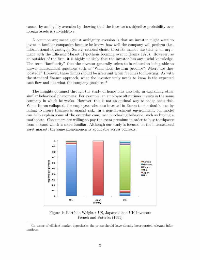
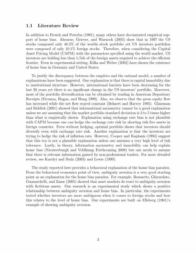
Equity Home Bias is a phenomenon in which investors over-invest in home country assetscompared to what the rational model predicts. Despite the fact that, in the past 4 years,foreign stocks have been outperforming domestic stocks on average, US investors stillmaintain a domestic-asset-heavy portfolio. Home bias is not limited to US investors butoccurs worldwide (Figure 1). There has been strong empirical support for the existenceof home bias paradox and many scholars have made various arguments trying to explainthis puzzle. The inflation rate, exchange rate, information asymmetry, and informationimmobility are some of the popular choices but none of these have been generally acceptedor empirically consistent. However, these explanations are all within a rational choiceframework. Here, we propose a behavioral framework, ambiguity aversion, to help betterunderstand the cause of equity market home bias. Simply put, we argue that ambiguityaversion inhibits people from investing in unfamiliar companies. Unlike previous studies,we use an experimental design with real world assets and test for ambiguity aversioninstead of using fictitious assets or simply showing home bias without an explanation.

Equity market home bias1 presents an interesting problem because the investors arebeing “irrational” in the sense that they are not investing in a pareto-optimal manner:there exists another portfolio allocation such that the investor does not face any higherrisk (variance) but receives higher expected return. If people are indeed being irrationalwith their portfolio selection, then this presents an arbitrage opportunity. In addition, theirrational behavior raises the question of why investors are not allocating risks efficiently.Our paper shows that 1) using real world assets there is home bias, and 2) the bias is

∗I owe many thanks to Ming Hsu, Colin Camerer, Peter Bossaerts, John O’Doherty, David Grether,Jaksa Cvitanic and Eileen Chou for their helpful comments and discussions. The experiments weregraciously funded by Colin Camerer. I also thank Walter Yuan for introducing me to the world of PHP,MySQL and Apache server. I am grateful to seminar participants at Caltech, ESA International Meetingand BDRM Conference. Existing errors are my sole responsibility.†Email: noah.myung@caltech.edu. Phone: 626-395-8772. Web: www.hss.caltech.edu/∼noah and at

the Naval Postgraduate School’s Graduate School of Business and Public Policy starting Fall 2009.1We will drop the term “equity” from here on out.

caused by ambiguity aversion by showing that the investor’s subjective probability overforeign assets is sub-additive.

A common argument against ambiguity aversion is that an investor might want toinvest in familiar companies because he knows how well the company will perform (i.e.,informational advantage). Surely, rational choice theorists cannot use that as an argu-ment with the Efficient Market Hypothesis looming over it (Fama 1970). However, asan outsider of the firm, it is highly unlikely that the investor has any useful knowledge.The term “familiarity” that the investor generally refers to is related to being able toanswer nontechnical questions such as “What does the firm produce? Where are theylocated?” However, these things should be irrelevant when it comes to investing. As withthe standard finance approach, what the investor truly needs to know is the expectedcash flow and not what the company produces.2

The insights obtained through the study of home bias also help in explaining othersimilar behavioral phenomena. For example, an employee often times invests in the samecompany in which he works. However, this is not an optimal way to hedge one’s risk.When Enron collapsed, the employees who also invested in Enron took a double loss byfailing to insure themselves against risk. In a non-investment environment, our modelcan help explain some of the everyday consumer purchasing behavior, such as buying atoothpaste. Consumers are willing to pay the extra premium in order to buy toothpastefrom a brand which is more familiar. Although our study is focused on the internationalasset market, the same phenomenon is applicable across contexts.

Figure 1: Portfolio Weights: US, Japanese and UK InvestorsFrench and Poterba (1991)

2In terms of efficient market hypothesis, the prices should have already incorporated relevant infor-mations.

2

1.1 Literature Review

In addition to French and Poterba (1991), many others have documented empirical sup-port of home bias. Ahearne, Griever, and Warnock (2003) show that in 1997 the USstocks composed only 48.3% of the worlds stock portfolio yet US investors portfolioswere composed of only 10.1% foreign stocks. Therefore, when considering the CapitalAsset Pricing Model (CAPM) with the parameters specified using the world market, USinvestors are holding less than 1/5th of the foreign assets required to achieve the efficientfrontier. Even in experimental setting, Kilka and Weber (2002) have shown the existenceof home bias in Germany and United States.

To justify the discrepancy between the empirics and the rational model, a number ofexplanations have been suggested. One explanation is that there is capital immobility dueto institutional structure. However, international barriers have been decreasing for thelast 30 years yet there is no significant change in the US investors’ portfolio. Moreover,most of the portfolio diversification can be obtained by trading in American DepositaryReceipts (Errunza, Hogan, and Hung 1999). Also, we observe that the gross equity flowhas increased while the net flow stayed constant (Bekaert and Harvey 1995). Glassmanand Riddick (2001) showed that informational asymmetry cannot be a good explanationunless we are assuming that the market portfolio standard deviation is 2 to 5 times higherthan what is empirically shown. Explanation using exchange rate bias is not plausiblewith CAPM because one can hedge the exchange rate risk by shorting risk free assets inforeign countries. Even without hedging, optimal portfolio shows that investors shoulddiversify even with exchange rate risk. Another explanation is that the investors aretrying to hedge the risk of inflation rate. However, Cooper and Kaplanis (1994) suggestthat this too is not a plausible explanation unless one assumes a very high level of risktolerance. Lastly, in theory, information asymmetry and immobility can help explainhome bias (Nieuwerburgh and Veldkamp Forthcoming 2008) but one needs to assumethat there is relevant information gained by non-professional traders. For more detailedreview, see Karolyi and Stulz (2003) and Lewis (1999).

The study reported here provides a behavioral explanation of the home bias paradox.From the behavioral economics point of view, ambiguity aversion is a very good startingpoint as an explanation for the home bias paradox. For example, Bossaerts, Ghirardato,Guanaschelli, and Zame (2005) showed that asset markets do react to ambiguity aversionwith fictitious assets. Our research is an experimental study which shows a positiverelationship between ambiguity aversion and home bias. In particular, the experimentstested whether investors are more ambiguous when it comes to foreign stocks and howthis relates to the level of home bias. Our experiments are built on Ellsberg (1961)’sexample of showing ambiguity aversion.

3

1.2 Agenda

We begin by introducing the theory behind the mean-variance model and its implications,followed by various theories of ambiguity aversion, and non-additive subjective probabil-ity model we used for the experimental design. We present experimental results directlyafter presenting the design for all six experiments. First two designs target decision-making over individual companies while the last two designs target decision-making overindices. We end with a summarizing conclusion.

4

2 Theory

A short review of ambiguity aversion and the mean-variance model is discussed in thefollowing two subsections. Readers who are familiar with the topic may go directly tothe experimental design section. However, our experimental design is heavily based onthe non-additive probability discussed in the Theory of Ambiguity Aversion section.

2.1 Mean-Variance Model and Empirical Data

We follow the argument made by Lewis (1999). The standard model used in finance isthe mean-variance model. The utility function is called the mean-variance utility whenit increases with respect to mean and decreases with respect to variance. In particular,it has the following form: U = U(EtWt+1, V ar(Wt+1)) where Wt is the wealth at timet, V ar(•) is the variance-covariance matrix and Et is the expectations operator takenat time t. Furthermore, assume that ∂U

∂Wt> 0 and ∂2U

∂W 2t< 0. Denote αt, βt as the

proportion of wealth held in domestic and foreign assets at time t, respectively. Henceαt + βt = 1. Define rt = (rDt , r

Ft ) as turn on domestic assets and foreign assets at

time t. For example, one may consider the following utility function with all the desiredproperties: Wt(1+Etrt+1)−γV ar(WtEtrt+1) where γ is the risk aversion parameter. Now,solving for the first order condition of the objective function, the optimal proportion offoreign holding is:

βt =(Etr

Ft+1 − EtrDt+1)/γ

var(rF − rD)+

σ2D − σ2

FD

var(rF − rD)(1)

where γ = −2WtU2

U1is the relative risk aversion.

Consider the result from Equation 1. As the level of relative risk aversion increases,foreign investment decreases. However, there is a bound on how little one should invest

in foreign companies. In particular, the bound isσ2

D−σ2FD

var(rF−rD), which is empirically greater

than zero. Table 1 shows how much one should hold in foreign assets for a given relativerisk aversion.

Using the empirical data provided from Table 1 and optimal foreign holdings byEquation 1, even as relative risk aversion goes to infinity, one should still invest 39.5%of his shares in foreign assets. However, we observe approximately only 8% of the totalinvestments are directed to foreign assets. Hence, using the mean-variance model, evenwith unrealistic amount of risk aversion, the level of home bias cannot be explained.

2.2 Theory of Ambiguity Aversion

Decision theorists have defined and modeled ambiguity in several ways. The most intu-itive way of defining ambiguity is that the individual is uncertain about the distributionof the risk (Knight 1921). More uncertain the individual is about the distribution implies

5

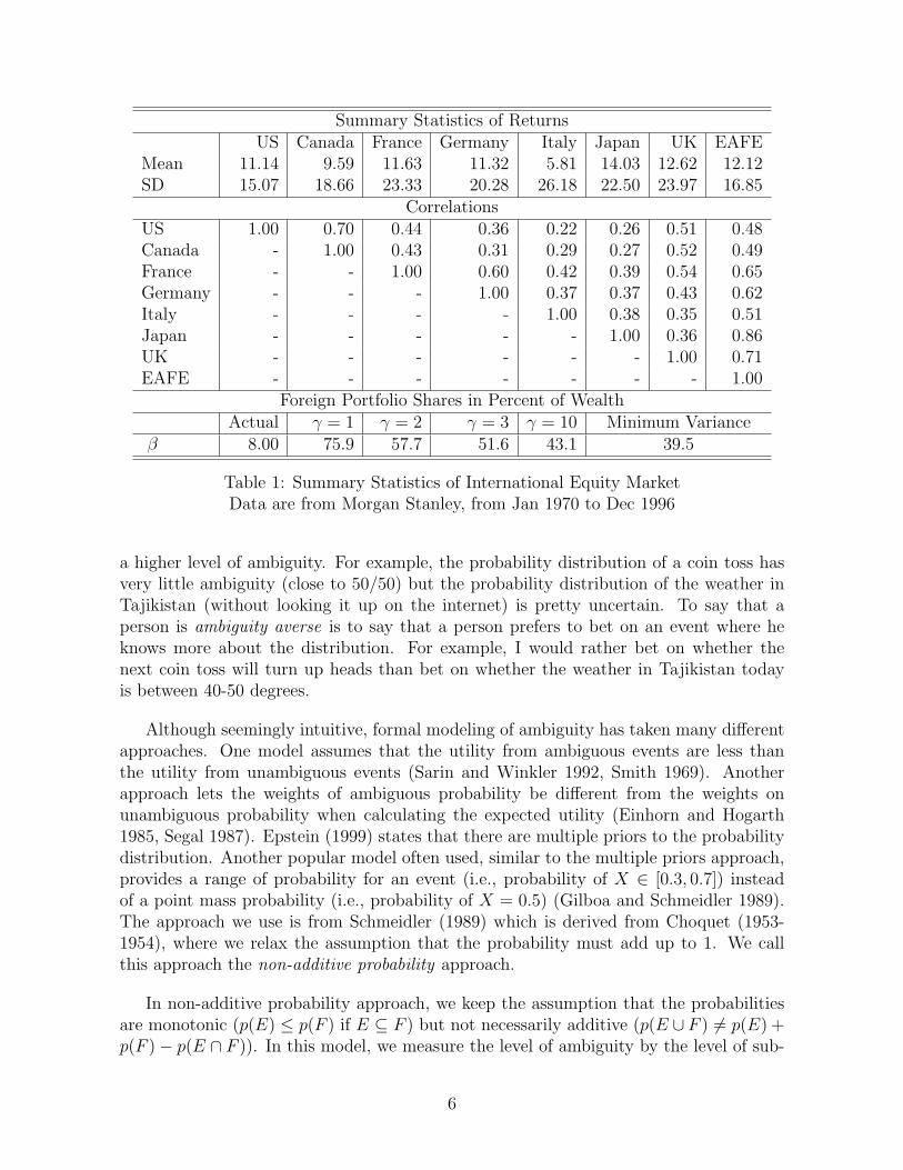
Summary Statistics of ReturnsUS Canada France Germany Italy Japan UK EAFE

Mean 11.14 9.59 11.63 11.32 5.81 14.03 12.62 12.12SD 15.07 18.66 23.33 20.28 26.18 22.50 23.97 16.85

CorrelationsUS 1.00 0.70 0.44 0.36 0.22 0.26 0.51 0.48Canada - 1.00 0.43 0.31 0.29 0.27 0.52 0.49France - - 1.00 0.60 0.42 0.39 0.54 0.65Germany - - - 1.00 0.37 0.37 0.43 0.62Italy - - - - 1.00 0.38 0.35 0.51Japan - - - - - 1.00 0.36 0.86UK - - - - - - 1.00 0.71EAFE - - - - - - - 1.00

Foreign Portfolio Shares in Percent of WealthActual γ = 1 γ = 2 γ = 3 γ = 10 Minimum Variance

β 8.00 75.9 57.7 51.6 43.1 39.5

Table 1: Summary Statistics of International Equity MarketData are from Morgan Stanley, from Jan 1970 to Dec 1996

a higher level of ambiguity. For example, the probability distribution of a coin toss hasvery little ambiguity (close to 50/50) but the probability distribution of the weather inTajikistan (without looking it up on the internet) is pretty uncertain. To say that aperson is ambiguity averse is to say that a person prefers to bet on an event where heknows more about the distribution. For example, I would rather bet on whether thenext coin toss will turn up heads than bet on whether the weather in Tajikistan todayis between 40-50 degrees.

Although seemingly intuitive, formal modeling of ambiguity has taken many differentapproaches. One model assumes that the utility from ambiguous events are less thanthe utility from unambiguous events (Sarin and Winkler 1992, Smith 1969). Anotherapproach lets the weights of ambiguous probability be different from the weights onunambiguous probability when calculating the expected utility (Einhorn and Hogarth1985, Segal 1987). Epstein (1999) states that there are multiple priors to the probabilitydistribution. Another popular model often used, similar to the multiple priors approach,provides a range of probability for an event (i.e., probability of X ∈ [0.3, 0.7]) insteadof a point mass probability (i.e., probability of X = 0.5) (Gilboa and Schmeidler 1989).The approach we use is from Schmeidler (1989) which is derived from Choquet (1953-1954), where we relax the assumption that the probability must add up to 1. We callthis approach the non-additive probability approach.

In non-additive probability approach, we keep the assumption that the probabilitiesare monotonic (p(E) ≤ p(F ) if E ⊆ F ) but not necessarily additive (p(E ∪ F ) 6= p(E) +p(F )− p(E ∩ F )). In this model, we measure the level of ambiguity by the level of sub-

6

additivity. In other words, while p(A) and p(B) are the likelihood of the events A andB, 1 − p(A) − p(B) measures the lack of “faith” in those likelihoods. Therefore, biggersub-additivity (1− p(A)− p(B)) implies higher levels of ambiguity.

Again, an interested reader may refer to Camerer and Weber (1992) for more detaileddiscussion and Epstein (1999) for more rigorous treatment.

7

3 Materials and Methods

A total of 55 people participated in this experiment; 47 were graduate and undergraduatestudents from the California Institute of Technology (Caltech) and 8 were not Caltechaffiliates. The participants were recruited using the Social Science Experimental Labo-ratory (SSEL) announcement system and public fliers. All participants were registeredsubjects with SSEL (signed a general consent form) and this experiment was approved asan exemption by the local research ethics committee. The experiment was conducted atthe SSEL located at Caltech, Pasadena, CA. The lab consists of 30 working computersdivided into a cubical setting. Subjects were physically prevented from viewing anotherstudent’s computer screen. The subjects were paid a show-up fee of $10 in addition toextra earnings based on their performance in the experiment.

The experimental designs dealing with individual companies (experiments 1-4) wereprogrammed using PHP3 and MySQL4 and are divided into four parts plus a survey sec-tion. The experimental designs dealing with indices (experiments 5-6) were programmedusing E-prime5 and are divided into two parts plus a survey section. Instructions weregiven prior to each section and were available both in print as well as on screen. Wequizzed the subjects after the instruction to insure they understood the experiment. Theinstructions provided to the participants are attached as an Appendix.

3www.php.net4www.mysql.com5www.pstnet.com/products/E-Prime

8

4 Control Experiment: Ellsberg Paradox

4.1 Experimental Summary and Motivation

We used the Ellsberg’s standard two urns and two colored balls experiment as the controltreatment (Ellsberg 1961). An ambiguous urn, urn 1, contains 100 balls with unknowndistribution of red and black. A risky urn, urn 2, contains 100 balls of which 50 arered and 50 are black. There is risk with urn 2 while uncertainty with urn 1. Thisbaseline treatment is conducted to obtain an approximation of which of the investors areambiguity averse and not ambiguity averse. The experimental structure below depictshow we go about in eliciting preference for ambiguity.

4.2 Experimental Structure

Ellsbergs experiment was administered to the investors in the following manner:

1. Investor is presented with two urns.

(a) Urn 1 contains 100 balls but the number of black or red balls is unknown.

(b) Urn 2 contains 100 balls, of which 50 are black and 50 are red.

2. Setting one: Investor is asked to pick from the following two gambles.

(a) $x dollar if red ball is drawn from urn 1.

(b) $x dollar if red ball is drawn from urn 2.

(c) Indifferent.

3. Setting two: Investor is asked to pick from the following two gambles.

(a) $x dollar if black ball is drawn from urn 1.

(b) $x dollar if black ball is drawn from urn 2.

(c) Indifferent.

We determined whether the investor is ambiguity averse or not by the choices hemakes in this Ellsberg experiment. In particular, if the investor chooses the gamble fromurn 2 (risky urn) in both settings, then we inferred that the investor was ambiguity averse.By choosing urn 2 in the first setting, it implies that the expected utility from gambletwo is greater than the expected utility from gamble one. If the investor chooses urn 2in the second setting, it implies that the expected utility from the gamble two is greaterthan gamble one. The following proposition will show why this leads to sub-additiveprobability, and therefore, ambiguity aversion.

Proposition 4.1 Under the expected utility maximization framework, choosing the riskyurn in both setting implies sub-additive probability measure.

9

Proof : Choosing gamble two in the first setting implies that

p(red ball|urn 2)u($x) > p(red ball|urn 1)u($x)

⇐⇒

p(red ball|urn 2) > p(red ball|urn 1) (2)

Choosing gamble two in the second setting implies that

p(black ball|urn 2)u($x) > p(black ball|urn 1)u($x)

⇐⇒

p(black ball|urn 2) > p(black ball|urn 1) (3)

Since urn 2 has 50 black and 50 red balls, it must be that p(black ball|urn 2)+p(red ball|urn 2) =1. From Equation 2 and 3, this implies that p(black ball|urn 1) + p(red ball|urn 1) < 1,which leads to a sub-additive probability measure.

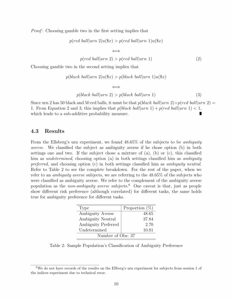
4.3 Results

From the Ellsberg’s urn experiment, we found 48.65% of the subjects to be ambiguityaverse. We classified the subject as ambiguity averse if he chose option (b) in bothsettings one and two. If the subject chose a mixture of (a), (b) or (c), this classifiedhim as undetermined, choosing option (a) in both settings classified him as ambiguitypreferred, and choosing option (c) in both settings classified him as ambiguity neutral.Refer to Table 2 to see the complete breakdown. For the rest of the paper, when werefer to an ambiguity averse subjects, we are referring to the 48.65% of the subjects whowere classified as ambiguity averse. We refer to the complement of the ambiguity aversepopulation as the non-ambiguity averse subjects.6 One caveat is that, just as peopleshow different risk preference (although correlated) for different tasks, the same holdstrue for ambiguity preference for different tasks.

Type Proportion (%)Ambiguity Averse 48.65Ambiguity Neutral 37.84Ambiguity Preferred 2.70Undetermined 10.81

Number of Obs: 37

Table 2: Sample Population’s Classification of Ambiguity Preference

6We do not have records of the results on the Ellberg’s urn experiment for subjects from session 1 ofthe indices experiment due to technical error.

10

5 Experiment 1: Portfolio Building

Definition 1 A derivative is called a Digital Option if it provides a fixed return afterreaching the strike price on the maturity date.

A digital option is often called an Arrow Security by economists. Consider the follow-ing example of a digital option. A digital call option with strike price k and payment r isdenoted as C(r, k) which pays zero if the stock price s < k and r if s ≥ k at the maturitydate. A digital put option with strike price k and payment r is denoted as P (r, k) whichpays zero if the stock price s > k and r if s ≤ k at the maturity date.

5.1 Setup for Individual Stocks, Experimental Summary, andMotivation

A motivation for this experiment is to test whether there is home bias in our sample, aswell as how the company choices are correlated with ambiguity aversion. We presenteda collection of 23 domestic and 27 foreign companies to the investor in a random order.These companies were all from the technology and semiconductor industry to minimizethe industry bias. In addition, these are companies listed as the 50 biggest companies inthe world with respect to their industry by Forbes 2004 magazine.7 Along with a companyname the investors were given their company’s ticker symbol, headquarter location, aswell as a brief list of company information which was provided by finance.google.com.Investors were asked to choose 15 companies to place a digital put option order and 15companies in a digital call option order. One option was given per company chosen bythe investor. These digital options had a maturity date of one week and strike price equalto the stock price at the day of the experiment. The investors were restricted from usingany tools other than the software required for the experiment. In addition, the investorswere not allowed to list a company for both a put and a call option. The investors werepaid based on the performance of their portfolio after the maturity date of the optionswhich paid $0.50 per option exercised.

This study answers two major questions. 1. Do investors show signs of home bias?2. What is the relationship between ambiguity aversion and home bias? We expect tosee the proportion of domestic companies chosen to be greater than 23/50 = 46%. Inaddition, we expect to see a positive correlation between the level of home biasness andambiguity.

7“Biggest company” was measured by a composite of sales, profits, assets, and market value. Thelist spans 51 countries and 27 industries.

11

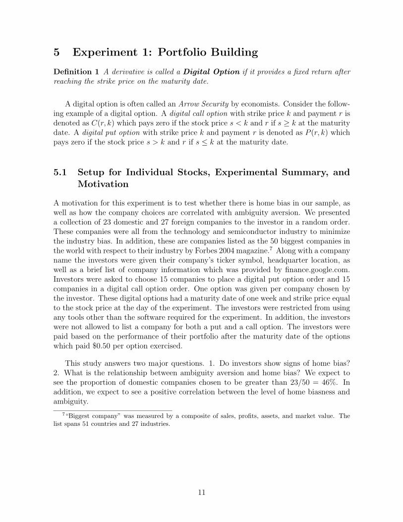
5.2 Results

Refer to Figure 2 for the average portfolio composition. We tested the hypothesis ofhome bias. On average, US companies comprised 52.70% (SE=3.05) of the call optionsand 49.21% (SE=2.54) of the put options, which gave a total of 50.95% (SE=1.30)investment in US companies. The investors were no more likely to choose call optionsfor US companies nor were they more likely to choose a put option for US companies.Given that the US companies consisted of only 46% of the possible companies availableto choose, this suggests that there is a home bias level of 4.95% where the differencesare significant at p < 0.01. This is a modest result but this may be caused by the factthat the experiment limits the industry choice and investors are required to choose 30companies.

Despite the fact that half of our subjects were considered to be ambiguity averse fromEllsberg’s experiment, we do not find a difference between the ambiguity averse and non-ambugity averse individual when it came to levels of home bias in their portfolio. In fact,we did not find any correlation between the result from the Ellsberg treatment and totalcomposition of one’s portfolio.

Figure 2: Share of US Companies in Portfolio

12

6 Experiment 2: Bond or Options?

6.1 Experimental Summary and Motivation

In this experimental design, the investor was shown one company at a time and was askedto choose one of the three gambles. Gamble 1 is to receive a bond which pays $1 one weeklater, Gamble 2 is to receive a digital call option with exercise value $1 and Gamble 3 isto receive a digital put option with exercise value $1. These options are identical to theprevious section minus the exercise value. However, the investor also faced a known riskin a sense that, having chosen gamble 1, he has P probability of actually receiving thebond. Also, by choosing a gamble 2 or 3, he has 1− P probability of actually receivingthe options. In this setting, the probability of receiving the security of choice becomesan implied cost: lower the probability implies a higher cost. (Refer to the experimentalinstructions for a detailed example.)

Each investor gets three domestic companies with P = 33%, three foreign companieswith P = 33%, three domestic companies with P = 29% and three foreign companieswith P = 29%. The companies were randomly selected for each investor. Investors werepaid based on the performance of every trial. After completing the entire experiment(after part 4), the investors were asked for the level of familiarity of these 12 companiesin the survey section.

Implied assumption is that the subjective probability belief over the stock prices isindependent of the probability of receiving the security (bond and options). With thisassumption, Proposition 2 claims that regardless of the belief over the performance ofthe stocks, choosing a bond will imply that the investor is exerting ambiguity aversion(via sub-additive probability).

Proposition 6.1 With any probability p < 33% in the above setting, selecting a bondwill lead to a sub-additive probability measure. In addition, as p decreases, the level ofsub-additivity of the probability measure increases, which implies higher level of ambiguityaversion.

Proof : Denote x as an event of receiving the bond and y as an event of receiving theoption. Denote v as an event of increase in price and w as an event of decrease in priceof the company’s stock. By assumption, p(y ∩ v) = p(y)p(v) and p(y ∩ w) = p(y)p(w).bond � put ⇐⇒ p(x)u($) > p(y ∩ v)u($)= p(y)p(v)u($) ⇒p(x) > p(y)p(v) hencep(x)/p(y) > p(v). Similarly, bond � call ⇐⇒ p(x)/p(y) > p(w). We observe thatp(w) + p(v) < 2p(x)/p(y). If p < 33%, then we have p(w) + p(v) <66/67 < 1, hence sub-additive probability measure. Notice as p decreases, 2p(x)/p(y) also decreases. Therefore,the level of sub-addivity of the probability measure increases as p decreases.

This section addresses four major questions: 1. Is there a difference in the level offamiliarity between domestic and foreign companies? 2. What is the relationship betweenthe level of familiarity and individual choices? 3. Are investors more likely to show higher

13

levels of ambiguity aversion in foreign companies compared to the domestic companies?And most importantly, 4. Are ambiguity averse investors more likely to choose bondsthan others?

6.2 Results

This section provides the most significant result out of all designs related to individualcompanies.

The familiarity of companies were coded using the following method. Investors wereasked during the survey section to state the level of familiarity from “never heard of it”,“not familiar”, “somewhat familiar”, “familiar”, and “very familiar.” We then coded thedummy variable using 1 to 5 from “never heard of it” to “very familiar” in increasingorder (µ = 2.18, σ = 1.30).

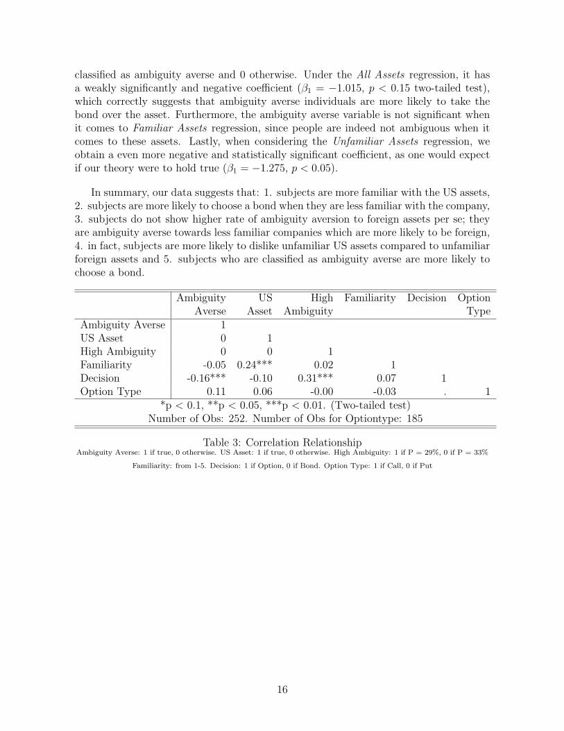
Table 3 presents a simple relationship from the experimental data. In particular, itaddresses whether there is a relationship between familiarity and individual choices. Wesee that investors are indeed more familiar with US companies than foreign companies(ρ = 0.24, p < 0.01). Next, we obtain a significant correlation between investmentdecision and ambiguity classification (ρ = −0.16, p < 0.01). This states that people whowere classified as ambiguity averse are more likely to choose to receive a bond in thisexperimental treatment. Table 3 suggests that the type of option chosen (call vs put)is not influenced by ambiguity aversion, country origin of asset, level of ambiguity, orfamiliarity.

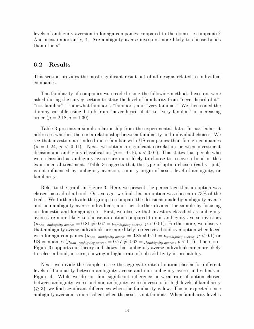
Refer to the graph in Figure 3. Here, we present the percentage that an option waschosen instead of a bond. On average, we find that an option was chosen in 73% of thetrials. We further divide the group to compare the decisions made by ambiguity averseand non-ambiguity averse individuals, and then further divided the sample by focusingon domestic and foreign assets. First, we observe that investors classified as ambiguityaverse are more likely to choose an option compared to non-ambiguity averse investors(µnon−ambiguity averse = 0.81 6= 0.67 = µambiguity averse, p < 0.01). Furthermore, we observethat ambiguity averse individuals are more likely to receive a bond over option when facedwith foreign companies (µnon−ambiguity averse = 0.85 6= 0.71 = µambiguity averse, p < 0.1) orUS companies (µnon−ambiguity averse = 0.77 6= 0.62 = µambiguity averse, p < 0.1). Therefore,Figure 3 supports our theory and shows that ambiguity averse individuals are more likelyto select a bond, in turn, showing a higher rate of sub-additivity in probability.

Next, we divide the sample to see the aggregate rate of option chosen for differentlevels of familiarity between ambiguity averse and non-ambiguity averse individuals inFigure 4. While we do not find significant difference between rate of option chosenbetween ambiguity averse and non-ambiguity averse investors for high levels of familiarity(≥ 3), we find significant differences when the familiarity is low. This is expected sinceambiguity aversion is more salient when the asset is not familiar. When familiarity level is

14

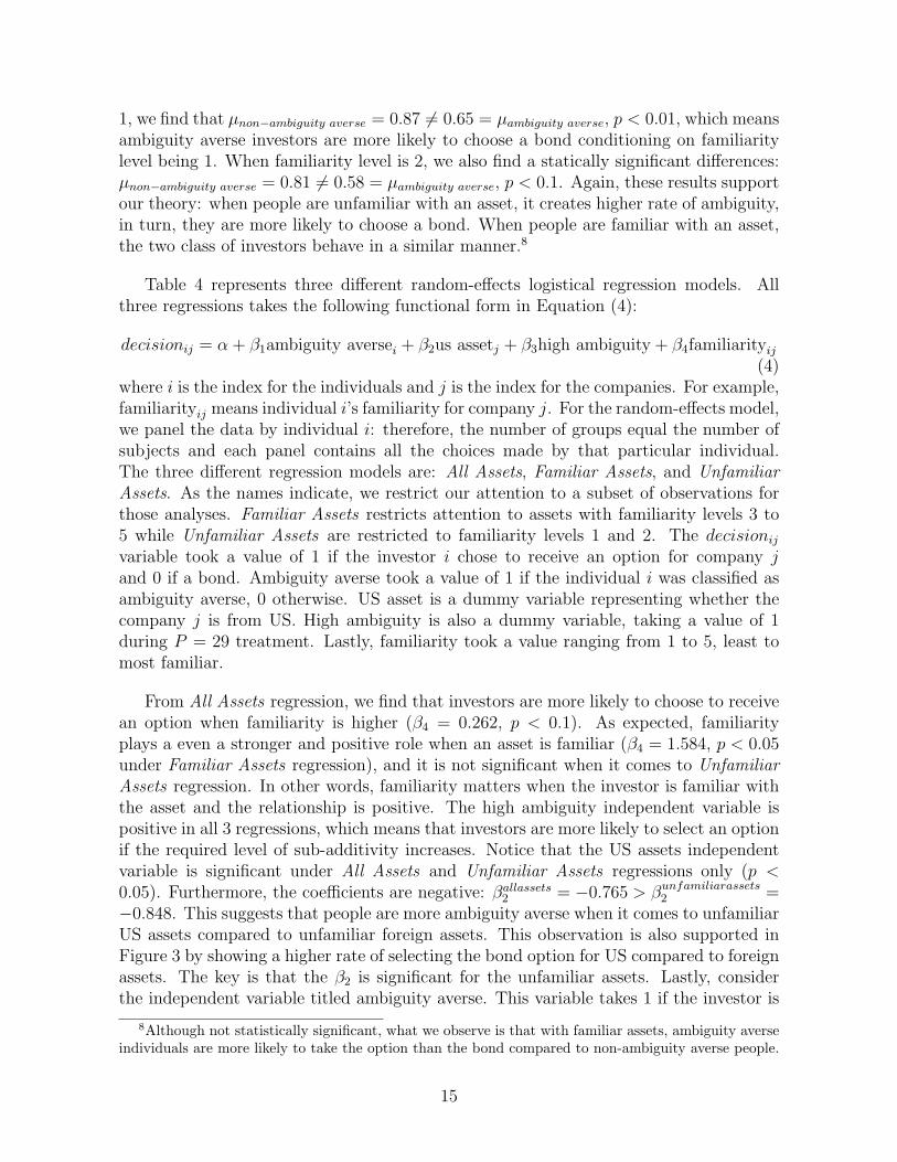
1, we find that µnon−ambiguity averse = 0.87 6= 0.65 = µambiguity averse, p < 0.01, which meansambiguity averse investors are more likely to choose a bond conditioning on familiaritylevel being 1. When familiarity level is 2, we also find a statically significant differences:µnon−ambiguity averse = 0.81 6= 0.58 = µambiguity averse, p < 0.1. Again, these results supportour theory: when people are unfamiliar with an asset, it creates higher rate of ambiguity,in turn, they are more likely to choose a bond. When people are familiar with an asset,the two class of investors behave in a similar manner.8

Table 4 represents three different random-effects logistical regression models. Allthree regressions takes the following functional form in Equation (4):

decisionij = α + β1ambiguity aversei + β2us assetj + β3high ambiguity + β4familiarityij(4)

where i is the index for the individuals and j is the index for the companies. For example,familiarityij means individual i’s familiarity for company j. For the random-effects model,we panel the data by individual i: therefore, the number of groups equal the number ofsubjects and each panel contains all the choices made by that particular individual.The three different regression models are: All Assets, Familiar Assets, and UnfamiliarAssets. As the names indicate, we restrict our attention to a subset of observations forthose analyses. Familiar Assets restricts attention to assets with familiarity levels 3 to5 while Unfamiliar Assets are restricted to familiarity levels 1 and 2. The decisionijvariable took a value of 1 if the investor i chose to receive an option for company jand 0 if a bond. Ambiguity averse took a value of 1 if the individual i was classified asambiguity averse, 0 otherwise. US asset is a dummy variable representing whether thecompany j is from US. High ambiguity is also a dummy variable, taking a value of 1during P = 29 treatment. Lastly, familiarity took a value ranging from 1 to 5, least tomost familiar.

From All Assets regression, we find that investors are more likely to choose to receivean option when familiarity is higher (β4 = 0.262, p < 0.1). As expected, familiarityplays a even a stronger and positive role when an asset is familiar (β4 = 1.584, p < 0.05under Familiar Assets regression), and it is not significant when it comes to UnfamiliarAssets regression. In other words, familiarity matters when the investor is familiar withthe asset and the relationship is positive. The high ambiguity independent variable ispositive in all 3 regressions, which means that investors are more likely to select an optionif the required level of sub-additivity increases. Notice that the US assets independentvariable is significant under All Assets and Unfamiliar Assets regressions only (p <0.05). Furthermore, the coefficients are negative: βallassets2 = −0.765 > βunfamiliarassets2 =−0.848. This suggests that people are more ambiguity averse when it comes to unfamiliarUS assets compared to unfamiliar foreign assets. This observation is also supported inFigure 3 by showing a higher rate of selecting the bond option for US compared to foreignassets. The key is that the β2 is significant for the unfamiliar assets. Lastly, considerthe independent variable titled ambiguity averse. This variable takes 1 if the investor is

8Although not statistically significant, what we observe is that with familiar assets, ambiguity averseindividuals are more likely to take the option than the bond compared to non-ambiguity averse people.

15

classified as ambiguity averse and 0 otherwise. Under the All Assets regression, it hasa weakly significantly and negative coefficient (β1 = −1.015, p < 0.15 two-tailed test),which correctly suggests that ambiguity averse individuals are more likely to take thebond over the asset. Furthermore, the ambiguity averse variable is not significant whenit comes to Familiar Assets regression, since people are indeed not ambiguous when itcomes to these assets. Lastly, when considering the Unfamiliar Assets regression, weobtain a even more negative and statistically significant coefficient, as one would expectif our theory were to hold true (β1 = −1.275, p < 0.05).

In summary, our data suggests that: 1. subjects are more familiar with the US assets,2. subjects are more likely to choose a bond when they are less familiar with the company,3. subjects do not show higher rate of ambiguity aversion to foreign assets per se; theyare ambiguity averse towards less familiar companies which are more likely to be foreign,4. in fact, subjects are more likely to dislike unfamiliar US assets compared to unfamiliarforeign assets and 5. subjects who are classified as ambiguity averse are more likely tochoose a bond.

Ambiguity US High Familiarity Decision OptionAverse Asset Ambiguity Type

Ambiguity Averse 1US Asset 0 1High Ambiguity 0 0 1Familiarity -0.05 0.24*** 0.02 1Decision -0.16*** -0.10 0.31*** 0.07 1Option Type 0.11 0.06 -0.00 -0.03 . 1

*p < 0.1, **p < 0.05, ***p < 0.01. (Two-tailed test)Number of Obs: 252. Number of Obs for Optiontype: 185

Table 3: Correlation RelationshipAmbiguity Averse: 1 if true, 0 otherwise. US Asset: 1 if true, 0 otherwise. High Ambiguity: 1 if P = 29%, 0 if P = 33%

Familiarity: from 1-5. Decision: 1 if Option, 0 if Bond. Option Type: 1 if Call, 0 if Put

16

Figure 3: Decision Comparison: By Ambiguity and Origin of Assets

Figure 4: Decision Comparison: By Ambiguity and FamiliarityAA: Ambiguity Averse. NA: Not Ambiguity Averse. Fi: Familiarity level i

17

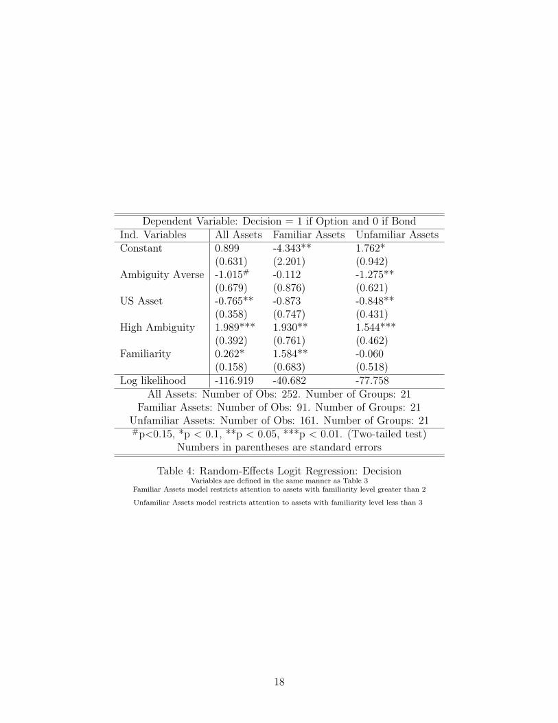
Dependent Variable: Decision = 1 if Option and 0 if BondInd. Variables All Assets Familiar Assets Unfamiliar AssetsConstant 0.899 -4.343** 1.762*

(0.631) (2.201) (0.942)Ambiguity Averse -1.015# -0.112 -1.275**

(0.679) (0.876) (0.621)US Asset -0.765** -0.873 -0.848**

(0.358) (0.747) (0.431)High Ambiguity 1.989*** 1.930** 1.544***

(0.392) (0.761) (0.462)Familiarity 0.262* 1.584** -0.060

(0.158) (0.683) (0.518)Log likelihood -116.919 -40.682 -77.758

All Assets: Number of Obs: 252. Number of Groups: 21Familiar Assets: Number of Obs: 91. Number of Groups: 21

Unfamiliar Assets: Number of Obs: 161. Number of Groups: 21#p<0.15, *p < 0.1, **p < 0.05, ***p < 0.01. (Two-tailed test)

Numbers in parentheses are standard errors

Table 4: Random-Effects Logit Regression: DecisionVariables are defined in the same manner as Table 3

Familiar Assets model restricts attention to assets with familiarity level greater than 2

Unfamiliar Assets model restricts attention to assets with familiarity level less than 3

18

7 Experiment 3: Company Preference

7.1 Experimental Summary and Motivation

In this part of the experiment, the investors are shown two companies (A and B) andasked to choose one of the three gambles: Gamble 1 : A outperforms B, Gamble 2 : Boutperforms A and Gamble 3: A equals B. The term outperform means that the percentchange in the company’s stock price is higher than the other companys percent changeone week from the day of the experiment. For the purpose of payment, we randomlyselected one of the trials the investor went through and paid $5 if he made the correctchoice.

The key to this experiment is how the two companies are populated. Recall that fromexperiment 1, the investor specified his portfolio. Using this portfolio, the experiment isprogrammed to ask for comparison between US companies with put requests and foreigncompanies with call requests. In addition, the experiment also asked for a comparisonbetween US companies with call requests and foreign companies with put requests. Giventhat the investor requested a put option for one company and a call option for anothercompany, he should take the gamble which states the call company will outperform theput company. If the investor selects the US company which he requested a put option forover the foreign company which he requested a call option for, by the proposition below,the investor is showing ambiguity aversion against the foreign company.

Proposition 7.1 After choosing a put option for company A and a call option for com-pany B, stating that company A will outperform company B leads to a sub-additivity inprobability measure.

Proof : Denote v as an event of increase in price and w as an event of decrease in priceof the company’s stock price. Having chosen a put option for company A implies thatp(w|A) > p(v|A). Having chosen a call option for company B implies that p(v|B) >p(w|B). Stating that company A will outperform company B implies that p(v|A) >p(v|B). Since p is a probability measure, highest p(v|A) can be is 1/2. Therefore,1/2 > p(v|B) > p(w|B) hence p(v|B) + p(w|B) < 1.

This design addresses the following major questions. 1. Do the investors consistentlyprefer the US companies over the foreign companies? 2. Are the investors who showedsigns of ambiguity aversion during the Ellsberg setting (experiment 1) more likely tochoose US (put) companies over foreign (call) companies?

7.2 Results

In short, we do not find any statistically significant results from this experimental study.

To support that there is sub-additive probability beliefs towards foreign companies,one would expect to see a higher rate of choosing US put over foreign call gambles

19

compared to choosing foreign put over US call gambles. In our data, when investors weremaking a decision between US put company and foreign call company, investors preferredthe US put over foreign call 22.59% (SE=4.58%) of the time (Figure 5). In other words,the investors exhibited sub-additivity 22.59% of the time. However, when faced with UScall and foreign put, investors preferred the foreign put 25.74% (SE=3.45%) of the time.The difference is not statistically significant.

As presented below, we further divided the observation by ambiguity category (Figure5), portfolio composition (Figure 6), and conducted various regression analyses (Table5). However, we did not find any significant result to support our theory.

The two possible explanation for the results we observed are: 1. familiarity and 2.risk hedging. The result we observe here may be due to higher familiarity of foreigncompanies shown over the US companies. The survey of familiarity of the companieschosen during the portfolio building section was not taken and cannot be tested.

Another possible explanation which we can infer from the data is that the investorswere hedging their risk. Since the mean share of US companies in the investor’s portfoliois 51%, we can split the investors into two types: US-heavy investors who have over51% of US companies in their portfolio and US-light investors who have less than 51%.Then, from Figure 6 we observe that among the US-heavy investors, they are much morelikely to prefer foreign put over US call (p < 0.1). However, this difference disappearswhen we only consider the US-light investors. Since the investors over-invested in USassets during the portfolio building section, they may have decided to under-invest incompany comparison section since these are exactly the same companies they previouslyinvested in. This type of experimental spill-over is a potential drawback of having thesame subject participate in the various treatments.

20

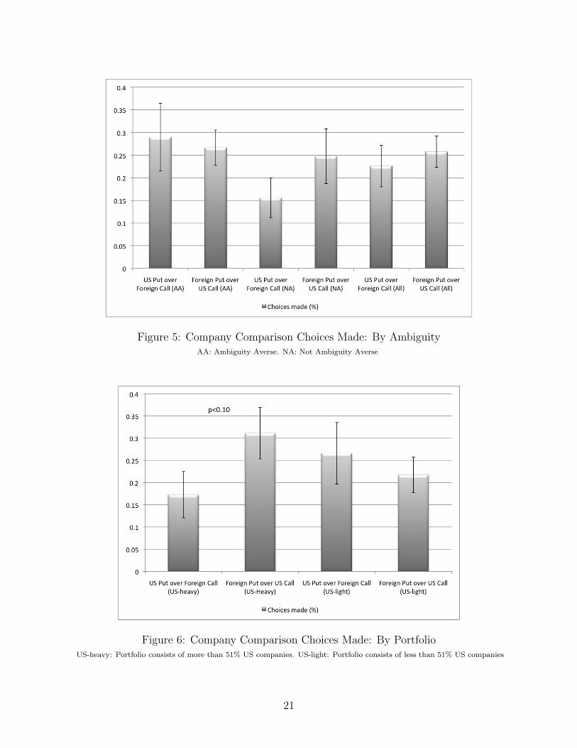
Figure 5: Company Comparison Choices Made: By AmbiguityAA: Ambiguity Averse. NA: Not Ambiguity Averse

Figure 6: Company Comparison Choices Made: By PortfolioUS-heavy: Portfolio consists of more than 51% US companies. US-light: Portfolio consists of less than 51% US companies

21

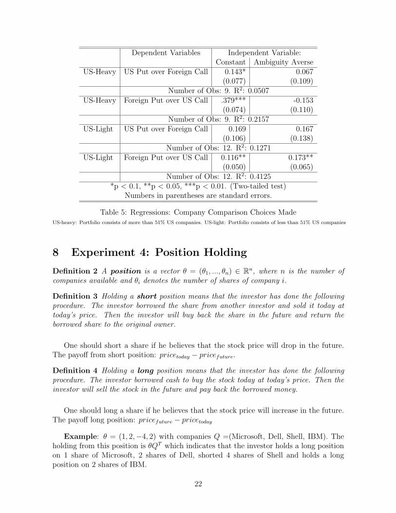
Dependent Variables Independent Variable:Constant Ambiguity Averse

US-Heavy US Put over Foreign Call 0.143* 0.067(0.077) (0.109)

Number of Obs: 9. R2: 0.0507US-Heavy Foreign Put over US Call .379*** -0.153

(0.074) (0.110)Number of Obs: 9. R2: 0.2157

US-Light US Put over Foreign Call 0.169 0.167(0.106) (0.138)

Number of Obs: 12. R2: 0.1271US-Light Foreign Put over US Call 0.116** 0.173**

(0.050) (0.065)Number of Obs: 12. R2: 0.4125

*p < 0.1, **p < 0.05, ***p < 0.01. (Two-tailed test)Numbers in parentheses are standard errors.

Table 5: Regressions: Company Comparison Choices MadeUS-heavy: Portfolio consists of more than 51% US companies. US-light: Portfolio consists of less than 51% US companies

8 Experiment 4: Position Holding

Definition 2 A position is a vector θ = (θ1, ..., θn) ∈ Rn, where n is the number ofcompanies available and θi denotes the number of shares of company i.

Definition 3 Holding a short position means that the investor has done the followingprocedure. The investor borrowed the share from another investor and sold it today attoday’s price. Then the investor will buy back the share in the future and return theborrowed share to the original owner.

One should short a share if he believes that the stock price will drop in the future.The payoff from short position: pricetoday − pricefuture.

Definition 4 Holding a long position means that the investor has done the followingprocedure. The investor borrowed cash to buy the stock today at today’s price. Then theinvestor will sell the stock in the future and pay back the borrowed money.

One should long a share if he believes that the stock price will increase in the future.The payoff long position: pricefuture − pricetoday

Example: θ = (1, 2,−4, 2) with companies Q =(Microsoft, Dell, Shell, IBM). Theholding from this position is θQT which indicates that the investor holds a long positionon 1 share of Microsoft, 2 shares of Dell, shorted 4 shares of Shell and holds a longposition on 2 shares of IBM.

22

Definition 5 The preference relation � satisfies the sure-thing principle if for anysubset E ⊂ S, (x1, ..., xS), (x′1, ..., x

′S), (x1, ..., xS) and (x′1, ..., x′S) are such that 1. For

all s /∈ E: xs = x′s and xs = x′s and 2. For all s ∈ E: xs = xs and x′s = x′s then(x1, ..., xS) � (x′1, ..., x′S) ⇐⇒ (x1, ..., xS) � (x′1, ..., x

′S).

8.1 Experimental Summary and Motivation

This experiment provides a method for testing the behavior of the investor in the multiplecompanies setting. This can be seen as investing in funds (such as mutual funds). In thisexperiment, the investor was asked to choose between taking a position that is shownor taking a bond. We will first discuss the concept behind this experiment and thendiscuss the exact implementation in the experimental structure section. This experimentis structured in the following manner. The investor was given a list of domestic posi-tions θD 6= (0, ...0) ∈ Rn. We then went through several iterations and determined theinvestor’s preference between the position and bond. Then we asked for the investor’spreference between θ = (θD, θF ) and a bond, where θF ∈ RM is a position in foreigncompanies. Again we went through several iterations in this setting. Lastly, we askedfor the investor’s preference between θ∗ = (θD,−θF ) and a bond. For the purpose ofpayment, an investor was paid from a randomly selected trial and was paid based onthe performance of the choice. If a position was selected, investor was paid based onthe performance of the position. We capped the earnings at $10 while the minimum wasbounded at $0 for the purpose of the experiment.

The data allows us to test whether the investor’s preferences are consistent. In otherwords, if the investor preferred θD over the bond but preferred the bond over θ = (θD, θF ),then he should prefer θ∗ = (θD,−θF ) over the bond. Otherwise, he is violating the sure-thing principle (Savage 1954).9 Same argument applies to the setting in which the investorprefers bond over θD, θ = (θD, θF ) over the bond and θ∗ = (θD,−θF ) over the bond.

8.2 Experimental Structure

This is divided into two phases. This section is written to provide a detailed explanationof what actually occurred during the experiment and may be skipped. The overview wasexplained in the previous section.

Phase 1: Single US and Single Foreign Company

1. Randomly select a US company listed under the call option from experiment 1.

(a) Ask for preference between the positive position of this company and a bond.

(b) Repeat this procedure until “position” choice is selected.

9Note that the violation of the sure-thing principle is a necessary but not a sufficient condition forambiguity aversion.

23

2. Randomly select a foreign company.

(a) Ask for preference between a positive position from the US company from 1-band negative position from the foreign company.

(b) Repeat this procedure until the “bond” choice is selected.

3. Reverse the position for the foreign company from 2-b and ask for preference be-tween the bond and the position.

Phase 2: Two US and Two Foreign Companies

1. Randomly select 2 US companies (without replacement) and give one a positiveand one a negative position.

(a) Compare the position with a bond.

(b) Repeat this 4 times.

2. Randomly select 2 foreign companies (without replacement), give one positive andone negative position, and pair this with one of the pairs from 1 (without replace-ment).

(a) Compare the position with a bond.

(b) Do this for all 4 pairs

3. Reverse the foreign company’s position from 2.

(a) Compare the position with a bond.

(b) Do this for all 4 pairs

This section addresses the following two major questions: 1. Do investors violate thesure-thing principle in the multiple companies setting? 2. If so, who are more likely toviolate the sure-thing principle?

8.3 Results

In this section, each investors provided 5 data points.10 Each data point is a binary resultof whether the investor violated the sure-thing principle. On average, investors violatedthe sure-thing principle 0.81 times (SE = 0.164), hence violated the sure thing principleapproximately 1 out of 5 times. These violations of sure-thing principle supports theargument that investors are ambiguity averse towards foreign assets.

Judging by the regression in Table 6, investors are more likely to violate the sure-thingprinciple in the position experiment if they are ambiguity averse (β = 4.920, p < 0.10).

10This is because a series of choices only provides 1 observation.

24

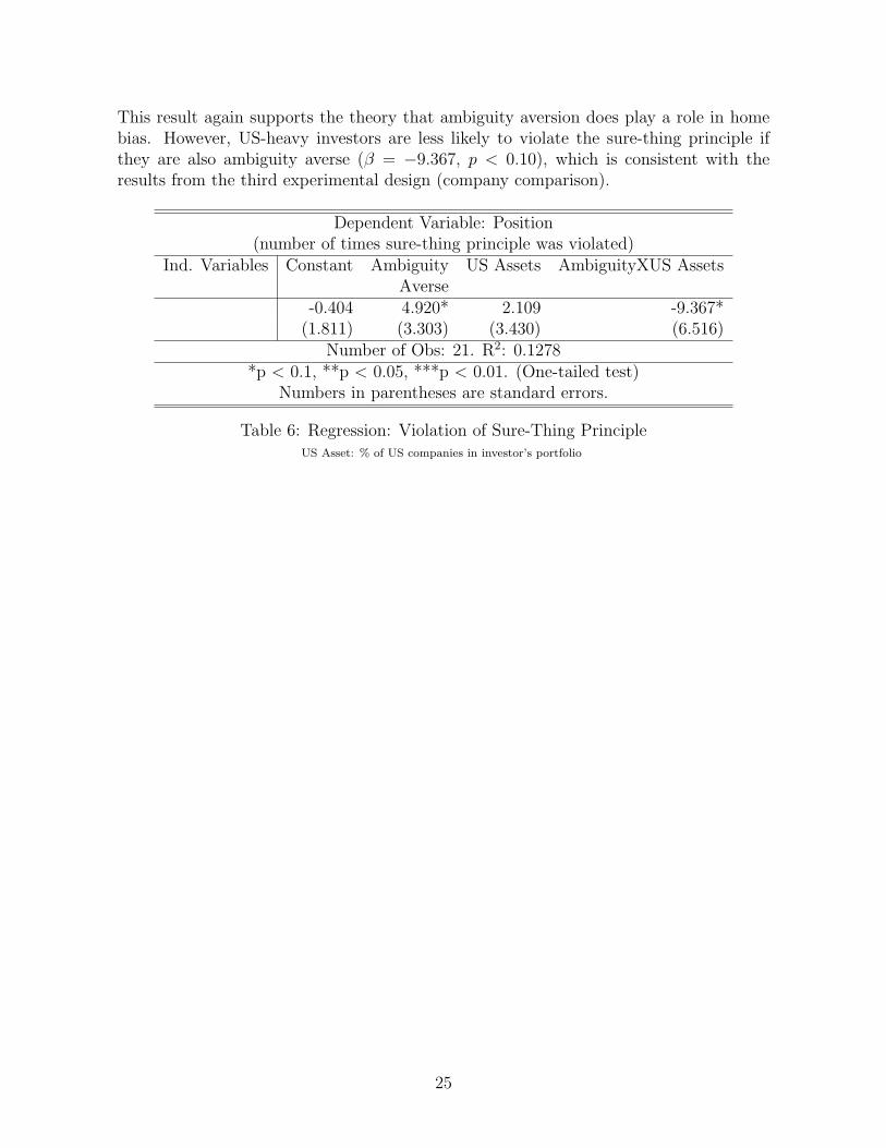
This result again supports the theory that ambiguity aversion does play a role in homebias. However, US-heavy investors are less likely to violate the sure-thing principle ifthey are also ambiguity averse (β = −9.367, p < 0.10), which is consistent with theresults from the third experimental design (company comparison).

Dependent Variable: Position(number of times sure-thing principle was violated)

Ind. Variables Constant Ambiguity US Assets AmbiguityXUS AssetsAverse

-0.404 4.920* 2.109 -9.367*(1.811) (3.303) (3.430) (6.516)

Number of Obs: 21. R2: 0.1278*p < 0.1, **p < 0.05, ***p < 0.01. (One-tailed test)

Numbers in parentheses are standard errors.

Table 6: Regression: Violation of Sure-Thing PrincipleUS Asset: % of US companies in investor’s portfolio

25

9 Experiment 5: Portfolio Building with Indices

9.1 Setup for Indices

Thus far we have focused on individual companies. We will shift our focus to indicesfor the next two experimental designs. Both setup and the experimental designs for theindices treatment are similar to the setup and the designs for the individual companies.There are several reasons why we need to consider both indices as well as individualcompanies. First, average investors tend to discuss and invest at a company level for dailytrading. However, when the average investors are planning a retirement plan throughfinancial advisors, they tend to invest in indices that are provided by the holding company.Secondly, people are more familiar with the companies than indices. In other words, thereis less of a company-level effect or company-level informational advantage, since indicesare composed of hundreds of different companies. Therefore, showing ambiguity aversionat the indices level may provide a stronger case of home bias. We are interested to learnwhether the ambiguity aversion is concentrated only at the individual company level orif it is also present at the index level.

For the indices treatment, we have selected 25 domestic and 25 foreign major indicesdefined by Bloomberg11 which varied in capitalization size as well as industry focus. Allthe investors were initially provided with a web-based prospectus. The prospectus wascreated using data provided by Bloomberg which included summarization of the index,value of the index for the past three months and their trading volume. The sampleinstructions, screen shots, and the list of indices are provided in the appendix.

9.2 Experimental Summary and Motivation

A motivation for this design is to test whether there is home bias in investment behaviorwhen dealing with indices. Investors were shown indices one by one and were asked tobuild their portfolio. A total of 25 domestic and 25 foreign indices were shown in arandom order. For each of the indices, they were given 3 options: buy the index, sell theindex, or receive a bond instead. The investors were paid based on the performance oftheir portfolio 7 days after the experiment was concluded. The payment structure was:

• If bond: $1.00

• If buy: $1.00 + (20× r)

• If sell: $1.00− (20× r)

where r is the return from the index. Although we did not use the term, they wereactually going long or short on the indices. The returns were multiplied by a factor of20 to stimulate long term investment.

11www.bloomberg.com

26

This study answers the following major questions: 1. Is there home bias when invest-ing in indices? 2. Are investors more familiar with US indices? 3. Are people more likelyto buy, sell, or receive a bond with US assets? 4. Do ambiguity averse investors havedifferent portfolio composition? Overall, what is the relationship between familiarity,ambiguity aversion, and investment choices?

9.3 Results

First, just as with the individual company treatment, investors are indeed more familiarwith the US indices than the foreign indices. When investors were asked to rate thefamiliarity of each index from 1-6, 1 being least and 6 being most familiar, the averagefamiliarity for US indices was 2.057 (SE = 0.032) and for foreign indices was 1.268(SE = 0.018), significantly different at p < 0.01. In fact, the correlation of familiarityis stronger for indices (ρ = 0.364, p < 0.01) than for individual companies (ρ = 0.24,p < 0.01).

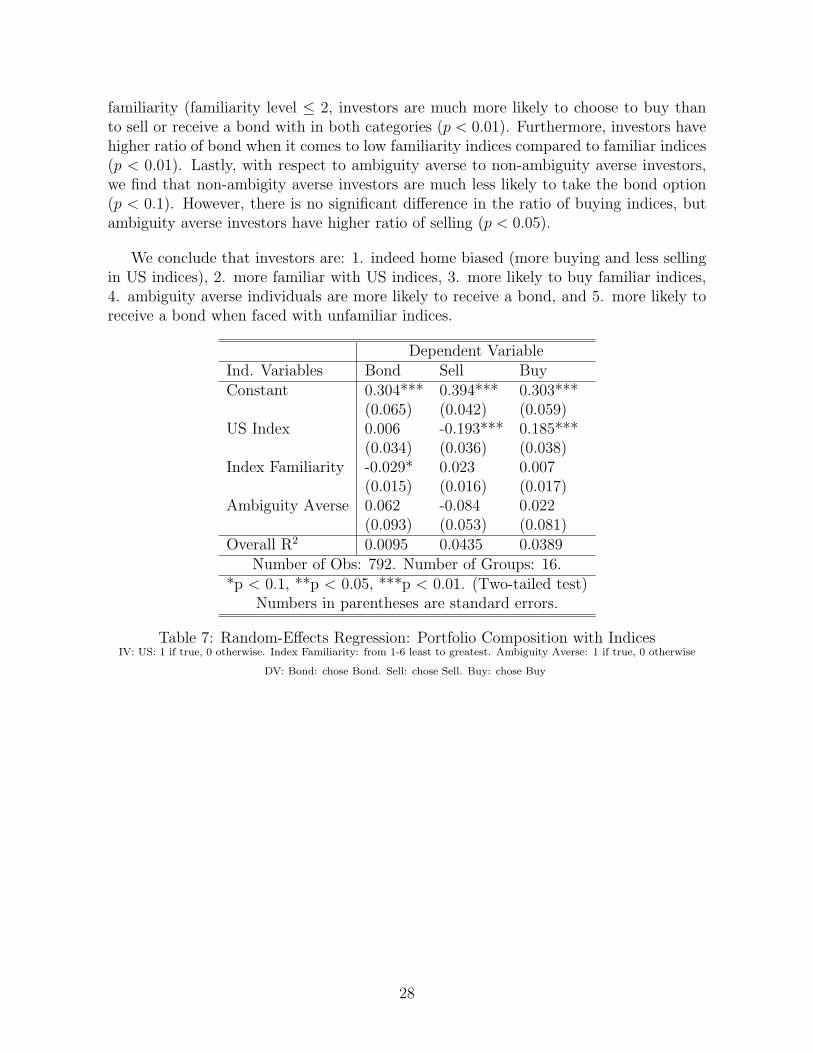
Three random-effects regressions are presented in Table 7 for Bond, Sell and Buy asthe functional form in Equation (5):

choiceij = α + β1us indexj + β2index familiarityij + β3ambiguity aversej (5)

where i is the index for the individuals and j is the index for the indices. Bond, Sell andBuy variables take 1 if the investor chose to receive the respective choice, 0 otherwise.US index is a dummy variable taking 1 for an US index. Index familiarity ranged from1-6 as stated above. The ambiguity averse variable takes 1 if the investor was classifiedas ambiguity averse via Ellsberg’s experiment, 0 otherwise.

The Bond regression’s significant coefficient is only for the index familiarity (β2 =−0.029, p < 0.1), which states that investors are more likely to take the bond choice ifthey are less familiar with the index. This is consistent with findings from the individualcompany treatment. The Sell regression and the Buy regressions also have one variablethat is statistically significant and it is for dummy variable US Index: β1 = −0.193,p < 0.01 for Sell and β1 = 0.185, p < 0.01 for Buy. This suggests that investors are muchmore likely to buy a US asset while less likely to sell a US asset. This is consistent witha home biased investor.

Figure 7 and Figure 8 presents the composition of investor’s portfolio. Overall, wefind that investors are more likely to buy than to receive a bond or sell (p < 0.01)although the difference in bond and selling is not significantly different. The biggestcontrast appears when comparing US indices to foreign indices. There is no significantdifferences when comparing the ratio of selling and bond for US indices but investorsare much more likely to buy US indices: composed over 50% of the portfolio (p < 0.01).However, the investment ratio is more evenly spread out when it comes to foreign indices.There is no significant difference when comparing buying and selling behavior for the USindices. When we divide the observation to high familiarity (familiarity level > 2) to low

27

familiarity (familiarity level ≤ 2, investors are much more likely to choose to buy thanto sell or receive a bond with in both categories (p < 0.01). Furthermore, investors havehigher ratio of bond when it comes to low familiarity indices compared to familiar indices(p < 0.01). Lastly, with respect to ambiguity averse to non-ambiguity averse investors,we find that non-ambigity averse investors are much less likely to take the bond option(p < 0.1). However, there is no significant difference in the ratio of buying indices, butambiguity averse investors have higher ratio of selling (p < 0.05).

We conclude that investors are: 1. indeed home biased (more buying and less sellingin US indices), 2. more familiar with US indices, 3. more likely to buy familiar indices,4. ambiguity averse individuals are more likely to receive a bond, and 5. more likely toreceive a bond when faced with unfamiliar indices.

Dependent VariableInd. Variables Bond Sell BuyConstant 0.304*** 0.394*** 0.303***

(0.065) (0.042) (0.059)US Index 0.006 -0.193*** 0.185***

(0.034) (0.036) (0.038)Index Familiarity -0.029* 0.023 0.007

(0.015) (0.016) (0.017)Ambiguity Averse 0.062 -0.084 0.022

(0.093) (0.053) (0.081)Overall R2 0.0095 0.0435 0.0389

Number of Obs: 792. Number of Groups: 16.*p < 0.1, **p < 0.05, ***p < 0.01. (Two-tailed test)

Numbers in parentheses are standard errors.

Table 7: Random-Effects Regression: Portfolio Composition with IndicesIV: US: 1 if true, 0 otherwise. Index Familiarity: from 1-6 least to greatest. Ambiguity Averse: 1 if true, 0 otherwise

DV: Bond: chose Bond. Sell: chose Sell. Buy: chose Buy

28

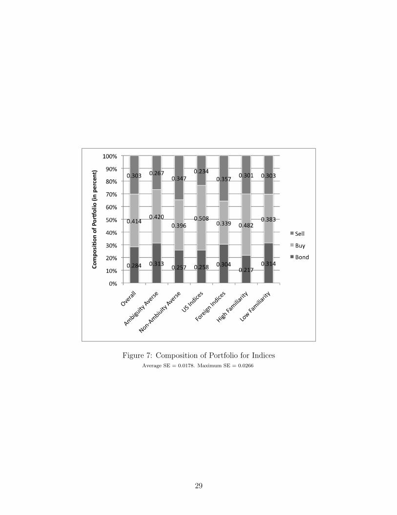
Figure 7: Composition of Portfolio for IndicesAverage SE = 0.0178. Maximum SE = 0.0266

29

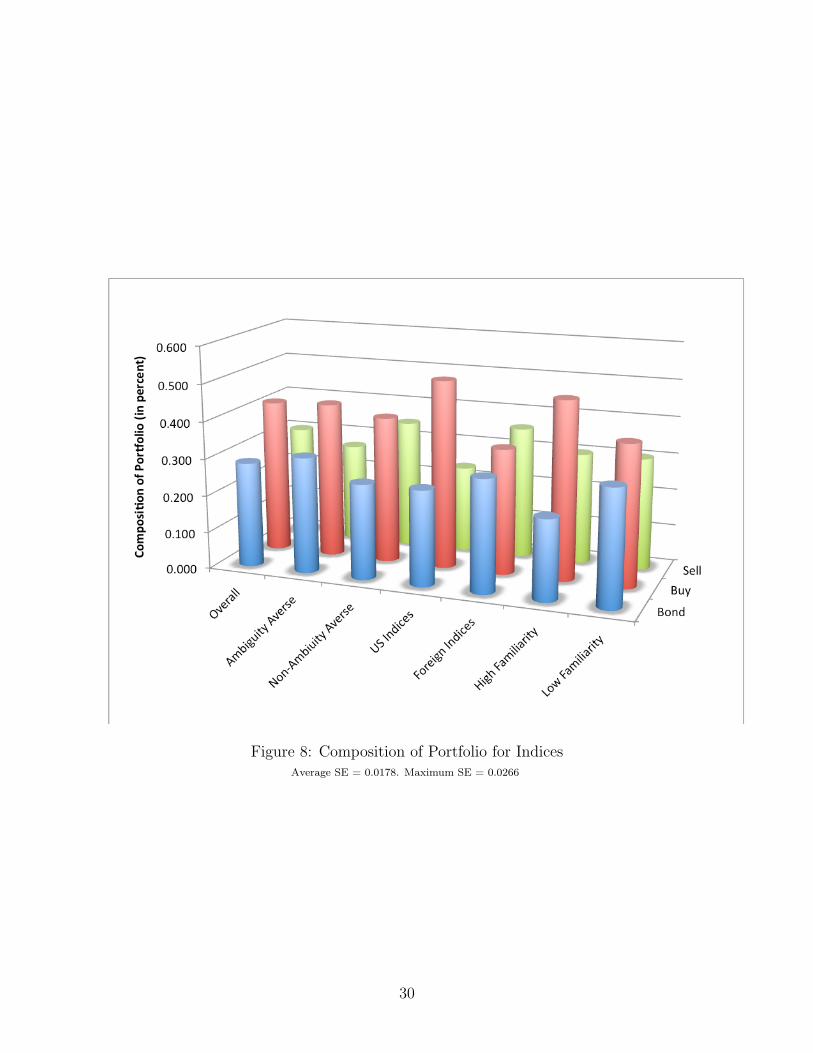
Figure 8: Composition of Portfolio for IndicesAverage SE = 0.0178. Maximum SE = 0.0266

30

10 Experiment 6: Bond or Options with Indices

10.1 Experimental Summary and Motivation

The design for this experiment is similar to the Bond or Options experiment under theindividual companies treatment. The investors were shown series of indices one at a timeand were given three possible choices just as in the stock treatment:

• Receive a bond which pays $1.00 with probability P .

• Receive a digital call option with exercise value of $1.00 with probability 1− P .

• Receive a digital put option with exercise value of $1.00 with probability 1− P .

However, there are two differences. First, we used indices instead of companies: 25domestic and 25 foreign, which were presented in random order. Second, we variedthe value of P , the known risk of receiving the actual derivative. Instead of focusingonly on P = 33% or P = 29% as in the individual companies treatment, we variedthe P ∈ {30, 32, 34, 36} for the indices treatment. Note that we are in a super-additivesubjective probability measure once P ≥ 34%.

This study answers the following major questions. What is the relationship betweenfamiliarity, ambiguity aversion, and investment choice?

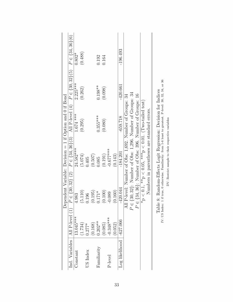
10.2 Results

Table 8 presents several random-effects logistical regression models. We regress sub-additive cases, super-additive cases, and all cases with the following two functional forms:

decisionij = α + β1us indexj + β2familiarityij + β3P-level (6)

anddecisionij = α + β2familiarityij (7)

Table 8 details the dependent variables. Consistent with our findings thus far, we findthat people are more likely to take the option with more familiar indices (see model (1),(2), (4), and (5)). The significance disappears once we focus only on the super-additivecases and this is expected (see model (3) and (6) in Table 8). Furthermore, model (1)shows that people are also more likely to take the option with a US index compared toforeign index.

Unlike the case with the individual companies, we do not get a strong result when an-alyzing the data by ambiguity and origin of indices (see Figure 9). The difference in rateof choosing an option is not statistically different when we divide our observation by US

31

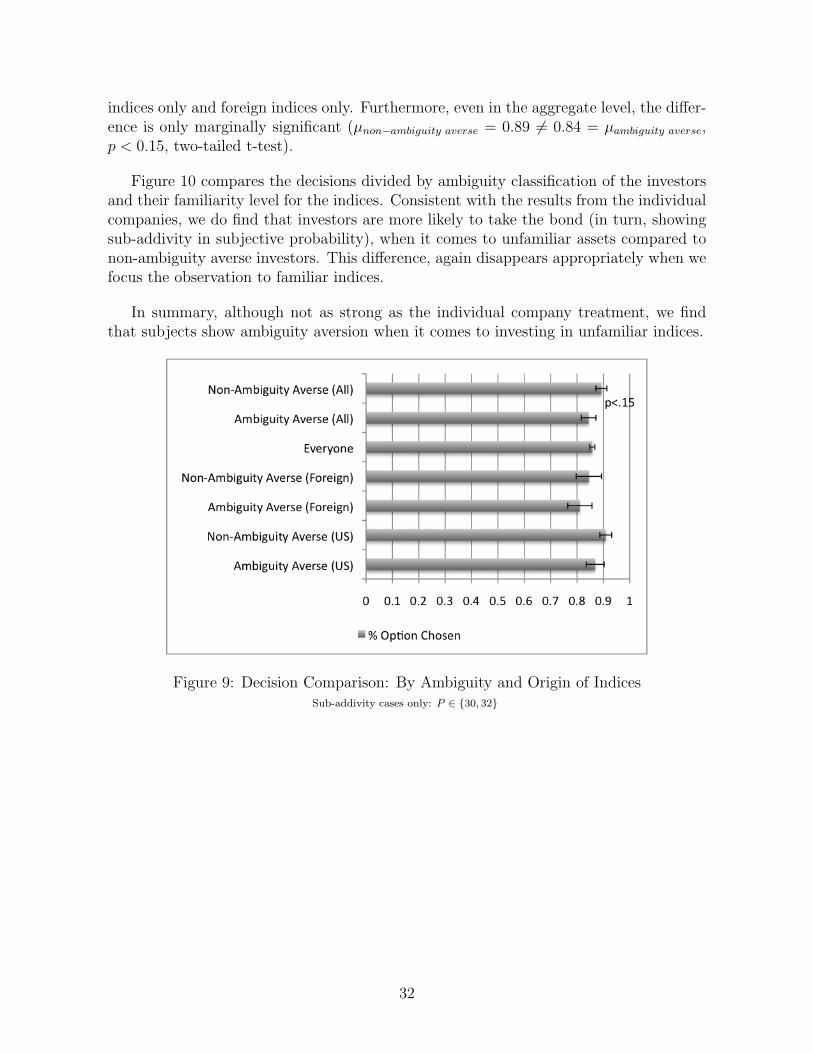
indices only and foreign indices only. Furthermore, even in the aggregate level, the differ-ence is only marginally significant (µnon−ambiguity averse = 0.89 6= 0.84 = µambiguity averse,p < 0.15, two-tailed t-test).

Figure 10 compares the decisions divided by ambiguity classification of the investorsand their familiarity level for the indices. Consistent with the results from the individualcompanies, we do find that investors are more likely to take the bond (in turn, showingsub-addivity in subjective probability), when it comes to unfamiliar assets compared tonon-ambiguity averse investors. This difference, again disappears appropriately when wefocus the observation to familiar indices.

In summary, although not as strong as the individual company treatment, we findthat subjects show ambiguity aversion when it comes to investing in unfamiliar indices.

Figure 9: Decision Comparison: By Ambiguity and Origin of IndicesSub-addivity cases only: P ∈ {30, 32}

32

Dep

enden

tV

aria

ble

:D

ecis

ion

=1

ifO

pti

onan

d0

ifB

ond

Ind.

Var

iable

sA

llP

-lev

el(1

)P∈{3

0,32}

(2)

P∈{3

4,36}(

3)A

llP

-lev

el(4

)P∈{3

0,32}(

5)P∈{3

4,36}(

6)C

onst

ant

13.0

45**

*4.

983

24.5

82**

*1.

674

***

2.22

5***

0.80

2*(1

.734

)(5

.110

)(5

.074

)(0

.295

)(0

.262

)(0

.488

)U

SIn

dex

0.27

7*0.

196

0.40

5(0

.168

)(0

.195

)(0

.507

)F

amilia

rity

0.20

2**

0.17

1*0.

085

0.35

5***

0.19

8**

0.19

2(0

.085

)(0

.100

)(0

.191

)(0

.080

)(0

.098

)0.

164

P-l

evel

-0.3

48**

*-0

.089

-0.6

77**

*(0

.052

)(0

.160

)(0

.143

)L

oglike

lihood

-627

.066

-420

.044

-184

.201

-659

.718

-420

.661

-196

.493

All

P-l

evel

:N

um

ber

ofO

bs:

1,69

2.N

um

ber

ofG

roups:

34P∈{3

0,32}:

Num

ber

ofO

bs:

1,29

6.N

um

ber

ofG

roups:

34P∈{3

4,36}:

Num

ber

ofO

bs:

396.

Num

ber

ofG

roups:

16*p

<0.

1,**

p<

0.05

,**

*p<

0.01

.(T

wo-

tailed

test

)N

um

ber

sin

par

enth

eses

are

stan

dar

der

rors

.

Tab

le8:

Ran

dom

-Eff

ects

Log

itR

egre

ssio

n:

Dec

isio

nfo

rIn

dic

esIV

:U

SIn

dex

:1

iftr

ue,

0oth

erw

ise.

Fam

ilia

rity

:fr

om

1-6

least

togre

ate

st.

P-l

evel

:30,

32,

34,

or

36

DV

:R

estr

ict

sam

ple

toth

eir

resp

ecti

ve

vari

ab

les

33

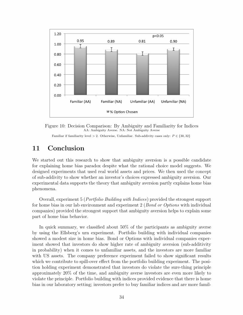
Figure 10: Decision Comparison: By Ambiguity and Familiarity for IndicesAA: Ambiguity Averse. NA: Not Ambiguity Averse

Familiar if familiarity level > 2. Otherwise, Unfamiliar. Sub-addivity cases only: P ∈ {30, 32}

11 Conclusion

We started out this research to show that ambiguity aversion is a possible candidatefor explaining home bias paradox despite what the rational choice model suggests. Wedesigned experiments that used real world assets and prices. We then used the conceptof sub-addivity to show whether an investor’s choices expressed ambiguity aversion. Ourexperimental data supports the theory that ambiguity aversion partly explains home biasphenomena.

Overall, experiment 5 (Portfolio Building with Indices) provided the strongest supportfor home bias in our lab environment and experiment 2 (Bond or Options with individualcompanies) provided the strongest support that ambiguity aversion helps to explain somepart of home bias behavior.

In quick summary, we classified about 50% of the participants as ambiguity averseby using the Ellsberg’s urn experiment. Portfolio building with individual companiesshowed a modest size in home bias. Bond or Options with individual companies exper-iment showed that investors do show higher rate of ambiguity aversion (sub-additivityin probability) when it comes to unfamiliar assets, and the investors are more familiarwith US assets. The company preference experiment failed to show significant resultswhich we contribute to spill-over effect from the portfolio building experiment. The posi-tion holding experiment demonstrated that investors do violate the sure-thing principleapproximately 20% of the time, and ambiguity averse investors are even more likely toviolate the principle. Portfolio building with indices provided evidence that there is homebias in our laboratory setting; investors prefer to buy familiar indices and are more famil-

34

iar with US indices. Lastly, Bond or Options with Indices experiment also showed that,even with indices, investors exhibit higher rate of ambiguity aversion when investing withunfamiliar indices.

Overall, the results provided here show positive support that ambiguity aversion asa partial explanation of home bias phenomenon. As Camerer and Karjalainen (1994)stated, methodologically, “this kind of work is difficult” and that even these modest size(sub-addivity of less than 5%) in ambiguity aversion “could have important economicconsequences” (pp. 348 - 349). Therefore, we are quite content with our modest resultprovided through our experiment, and hopeful for future research.

35

12 Appendix

12.1 Instructions for Individual Companies

The following 4 pages are sample instructions used in the experiment.

36

1

Inst

ruct

ion

prov

ided

to th

e st

uden

ts.

Thes

e in

stru

ctio

ns w

ere

hand

ed o

ut o

ne se

ctio

n at

a ti

me

Exp

erim

ent O

verv

iew

You

are

abo

ut to

par

ticip

ate

in a

n ex

perim

ent i

n th

e ec

onom

ics o

f dec

isio

n m

akin

g. If

you

list

en c

aref

ully

an

d m

ake

good

dec

isio

ns, y

ou c

ould

ear

n a

cons

ider

able

am

ount

of m

oney

that

will

be

paid

to y

ou in

cas

h or

che

ck a

t the

end

of t

he e

xper

imen

t (7

days

from

toda

y).

You

will

not

be

paire

d w

ith a

ny o

ther

indi

vidu

al. I

n ad

ditio

n, n

o ot

her p

erso

n's d

ecis

ion

will

influ

ence

you

r ou

tcom

e. A

ll yo

ur c

hoic

es w

ill b

e re

cord

ed to

day

and

your

out

com

e w

ill b

e re

aliz

ed o

ne w

eek

from

toda

y.

The

rule

s for

the

expe

rimen

t are

as f

ollo

ws.

Do

not t

alk

or c

omm

unic

ate

with

oth

er p

artic

ipan

ts. I

f you

are

us

ing

a co

mpu

ter,

do n

ot u

se a

ny so

ftwar

e ot

her t

han

that

is e

xplic

itly

requ

ired

by th

e ex

perim

ent.

You

are

no

t allo

wed

to b

row

se th

e in

tern

et o

r che

ck e

mai

ls, e

tc. I

f you

are

vio

late

thes

e ru

les,

you'

ll be

ask

ed to

le

ave

with

out p

ay. F

eel f

ree

to a

sk q

uest

ions

by

rais

ing

your

han

d or

sign

alin

g to

the

expe

rimen

ter.

Paym

ent:

You

will

rece

ive

a sh

ow-u

p fe

e of

$10

toda

y. A

t the

end

of t

oday

's se

ssio

n, y

ou c

an a

rran

ge to

ei

ther

pic

k up

the

addi

tiona

l ear

ning

s in

cas

h in

per

son

at B

axte

r Hal

l, R

oom

6 o

r hav

e a

chec

k m

aile

d to

yo

u.

The

Proc

ess w

ill n

ow b

e ex

plai

ned

in d

etai

l.

The

Pro

cess

This

exp

erim

ent i

s div

ided

into

four

par

ts p

lus a

surv

ey se

ctio

n.

Part

1. P

ortfo

lio B

uild

ing

In th

is p

art o

f the

exp

erim

ent,

you

will

be

show

n a

list o

f com

pani

es a

nd b

e as

ked

to b

uild

a p

ortfo

lio. A

ll th

e co

mpa

nies

are

from

the

tech

nolo

gy o

r sem

icon

duct

or in

dust

ry a

nd a

re c

onsi

dere

d to

be

one

of th

e to

p 50

big

gest

com

pani

es in

the

wor

ld w

ith re

spec

t to

thei

r ind

ustry

by

Forb

es. I

nclu

ded

in th

e co

mpa

ny li

st a

re

the

com

pany

nam

e, c

ompa

ny ti

cker

sym

bol,

loca

tion

of th

e he

adqu

arte

rs a

nd a

brie

f inf

orm

atio

n ab

out t

he

com

pany

pro

vide

d by

fina

nce.

goog

le.c

om. I

n th

is p

artic

ular

por

tfolio

, you

'll b

e as

ked

to c

hoos

e 15

co

mpa

nies

in w

hich

you

wis

h to

rece

ive

call

optio

ns a

nd 1

5 co

mpa

nies

in w

hich

you

wis

h to

rece

ive

put

optio

ns. D

etai

ls a

bout

thes

e op

tions

will

be

expl

aine

d be

low

. You

will

rece

ive

one

call

optio

n pe

r com

pany

yo

u lis

t und

er th

e ca

ll op

tion

box.

You

will

rece

ive

one

put o

ptio

n pe

r com

pany

you

list

und

er th

e pu

t op

tion

box.

You

can

not u

se th

e sa

me

com

pany

twic

e (m

eani

ng, i

f you

requ

este

d a

call

optio

n on

Mic

roso

ft,

you

cann

ot re

ques

t a p

ut o

ptio

n on

it a

s wel

l). W

hen

inse

rting

the

com

pani

es, p

leas

e in

sert

the

com

pany

sy

mbo

l sep

arat

ed b

y co

mm

a. D

o no

t pla

ce a

com

ma

afte

r the

last

sym

bol.

See

scre

en sh

ow b

elow

for a

n ex

ampl

e.

2

Abov

e is

the

sam

ple

of th

e co

mpa

ny li

st. B

elow

is th

e sa

mpl

e of

por

tfolio

bui

ldin

g se

ctio

n.

Opt

ions

: Pu

t opt

ion

will

giv

e yo

u $0

.50

if th

e st

ock

pric

e of

the

com

pany

one

wee

k fr

om to

day

is lo

wer

th

an th

e st

ock

pric

e to

day.

Cal

l opt

ion

will

giv

e yo

u $0

.50

if th

e st

ock

pric

e of

the

com

pany

one

wee

k fr

om

toda

y is

hig

her t

han

the

stoc

k pr

ice

toda

y. Y

ou w

ill b

e pa

id $

0.50

rega

rdle

ss o

f the

type

of o

ptio

n yo

u ho

ld

if th

e st

ock

pric

e on

e w

eek

from

toda

y is

the

sam

e as

toda

y's p

rice.

Oth

erw

ise,

you

will

rece

ive

noth

ing.

Payo

ff: Y

ou w

ill b

e pa

id b

ased

on

how

you

r ent

ire p

ortfo

lio p

erfo

rms o

ne w

eek

from

toda

y.

The

term

"to

day'

s sto

ck p

rice"

is th

e la

st tr

adin

g pr

ice

of th

e co

mpa

ny st

ock

colle

cted

from

fin

ance

.yah

oo.c

om a

nd w

ww

.tse.

or.jp

. Thi

s pric

e w

as re

cord

ed a

t noo

n to

day

(PST

). "P

rice

one

wee

k fr

om

toda

y" is

the

last

trad

ing

pric

e of

the

com

pany

stoc

k co

llect

ed fr

om fi

nanc

e.ya

hoo.

com

and

ww

w.ts

e.or

.jp 7

da

ys fr

om to

day,

12:

00PM

(PST

). Pl

ease

not

e th

at fi

nanc

e.ya

hoo.

com

has

a 1

0-20

min

ute

dela

y on

the

quot

es. H

ence

, at n

oon,

if th

e la

st tr

ade

post

ed is

11:

45A

M, t

hat i

s the

pric

e w

e w

ill b

e us

ing.

ww

w.ts

e.or

.jp

will

be

used

for c

ompa

nies

that

are

not

list

ed w

ith th

e ex

chan

ges f

rom

fina

nce.

yaho

o.co

m a

nd it

als

o ha

s 10

-20

min

ute

dela

y.

3

Exam

ple:

Sup

pose

you

are

par

ticip

atin

g on

the

expe

rimen

t on

Oct

1st

. You

cho

se a

put

opt

ion

for G

oogl

e.

The

last

trad

ing

pric

e po

sted

on

finan

ce.y

ahoo

.com

at n

oon

for G

oogl

e is

$40

0. S

even

day

s fro

m n

ow, O

ct

8th,

12:

00PM

, the

last

trad

ing

pric

e po

sted

on

finan

ce.y

ahoo

.com

for G

oogl

e is

$40

1 w

hich

is g

reat

er th

an

$400

. Sin

ce y

ou c

hose

a p

ut o

ptio

n, y

ou w

ill n

ot b

e pa

id. H

owev

er, i

f the

last

trad

ing

pric

e po

sted

on

finan

ce.y

ahoo

.com

for G

oogl

e is

$40

0 or

bel

ow, t

hen

you

will

be

able

to e

xerc

ise

your

opt

ion

and

rece

ive

$0.5

0.

Any

que

stio

ns?

Part

2. B

ond

or O

ptio

ns?

In th

is p

art o

f the

exp

erim

ent,

you

will

be

show

n on

e co

mpa

ny n

ame

at a

tim

e an

d be

ask

ed w

heth

er y

ou

wis

h to

take

the

bond

(whi

ch p

ays $

1), p

ut o

ptio

n or

a c

all o

ptio

n. T

hese

opt

ions

are

iden

tical

to th

e op

tions

in

par

t 1 a

nd w

ill p

ay $

1 if

exer

cise

d. A

bon

d is

a ri

sk fr

ee a

sset

whi

ch w

ill p

ay y

ou $

1 in

depe

nden

t of t

he

stoc

k pr

ice.

In th

is se

ctio

n, y

ou a

re a

lso

give

n a

butto

n "c

lick

here

to v

iew

com

pany

info

". P

ress

this

but

ton

and

you

will

be

give

n th

e co

mpa

ny in

fo fo

r the

se sp

ecifi

c co

mpa

nies

. See

the

scre

en sh

ow b

elow

for a

n ex

ampl

e.

Payo

ff: Y

ou w

ill b

e pa

id b

ased

on

the

outc

ome

of e

very

tria

l in

this

sect

ion.

How

ever

, in

this

sect

ion,

you

are

not

gua

rant

eed

to re

ceiv

e a

bond

or a

n op

tion.

You

will

be

give

n th

e pr

obab

ility

of r

ecei

ving

the

choi

ce y

ou se

lect

. In

the

abov

e ex

ampl

e, if

you

cho

ose

to re

ceiv

e a

bond

, you

ha

ve 3

3% c

hanc

e of

act

ually

rece

ivin

g it.

If y

ou d

o re

ceiv

e it,

you

'll b

e pa

id $

1 re

gard

less

of w

hat h

appe

ns

to th

e co

mpa

ny's

stoc

k pr

ice.

Oth

erw

ise,

you

will

rece

ive

$0. I

f you

cho

ose

to re

ceiv

e a

call

optio

n, th

en

you

have

a 6

7% c

hanc

e of

rece

ivin

g it

and

33%

cha

nce

of re

ceiv

ing

noth

ing.

Not

e th

at w

hen

you

do

actu

ally

rece

ive

a pu

t opt

ion,

you

are

not

gua

rant

eed

to b

e pa

id $

1 un

less

the

stoc

k pr

ice

one

wee

k fr

om

toda

y is

less

than

toda

y's p

rice.

See

the

tabl

e be

low

to g

et a

bet

ter u

nder

stan

ding

of t

he p

ayof

f.

If y

ou se

lect

a

Bon

d To

day'

s sto

ck p

rice

is le

ss th

an n

ext w

eek'

s st

ock

pric

e To

day'

s sto

ck p

rice

is g

reat

er th

an n

ext

wee

k's s

tock

pric

e 33

% c

hanc

e $1

$1

67

% c

hanc

e $0

$0

If

you

sele

ct a

Cal

l op

tion

Toda

y's s

tock

pric

e is

less

than

nex

t w

eek'

s sto

ck p

rice

Toda

y's s

tock

pric

e is

gre

ater

than

nex

t w

eek'

s sto

ck p

rice

33%

cha

nce

$0

$0

67%

cha

nce

$0

$1

4

If y

ou se

lect

a P

ut

optio

n To

day'

s sto

ck p

rice

is le

ss th

an n

ext

wee

k's s

tock

pric

e To

day'

s sto

ck p

rice

is g

reat

er th

an n

ext

wee

k's s

tock

pric

e 33

% c

hanc

e $0

$0

67

% c

hanc

e $1

$0

This

is h

ow th

e "c

hanc

e" is

det

erm

ined

in th

is se

ctio

n. If

it st

ates

that

ther

e is

a 4

5% c

hanc

e of

rece

ivin

g a

bond

, it m

eans

the

follo

win

g: w

e w

ill u

se a

rand

om n

umbe

r gen

erat

or w

hich

giv

es a

num

ber f

rom

1 -

100.

If

the

num

ber g

iven

is fr

om 1

- 45

, you

will

rece

ive

the

bond

. Oth

erw

ise,

you

will

not

. Aga

in, i

f it s

tate

s th

at th

ere

is a

55%

cha

nce

of re

ceiv

ing

an o

ptio

n, it

mea

ns th

e fo

llow

ing:

we

will

use

a ra

ndom

num

ber

gene

rato

r whi

ch g

ive

a nu

mbe

r fro

m 1

- 10

0. If

the

num

ber i

s fro

m 4

6 - 1

00, y

ou w

ill re

ceiv

e th

e op

tion.

Ea

ch tr

ials

are

inde

pend

ent o

f eac

h ot

her.

This

mea

ns th

at w

e w

ill ru

n th

e ra

ndom

num

ber g

ener

ator

eac

h tim

e fo

r eac

h tri

al y

ou h

ave

in th

is se

ctio

n.

Any

que

stio

ns?

Part

3. C

ompa

ny P

refe

renc

e

In th

is p

art o

f the

exp

erim

ent,

you'

ll be

show

n tw

o co

mpa

ny n

ames

(A a

nd B

) and

will

be

give

n th

ree

gam

bles

to c

hoos

e fr

om (s

ee sc

reen

shot

bel

ow).

Firs

t cho

ice

is a

bet

that

com

pany

A w

ill o

ut p

erfo

rm

com

pany

B in

one

wee

k fr

om n

ow. N

ext c

hoic

e is

a b

et th

at c

ompa

ny B

will

out

perf

orm

com

pany

A in

one

w

eek

from

now

. Las

t cho

ice

is a

bet

that

com

pany

A a

nd B

will

per

form

the

sam

e. Y

ou a

re a

lso

give

n a

butto

n "c

lick

here

to v

iew

com

pany

info

". P

ress

this

but

ton

and

you

will

be

give

n th

e co

mpa

ny in

fo fo

r th

ese

spec

ific

com

pani

es.

Payo

ff: U

sing

a ra

ndom

num

ber g

ener

ator

, we

will

rand

omly

sele

ct o

ne o

f the

tria

ls. Y

ou w

ill b

e pa

id

base

d on

the

perf

orm

ance

of t

he tr

ial s

elec

ted:

if th

e ga

mbl

e yo

u ch

ose

is th

e w

inne

r, yo

u w

ill re

ceiv

e $5

. O

ther

wis

e, y

ou'll

rece

ive

noth

ing.

The

term

"ou

tper

form

" is

def

ined

as f

ollo

ws:

com

pany

A o

ut p

erfo

rms c

ompa

ny B

if a

nd o

nly

if th

e in

crea

se in

per

cent

age

of th

e do

llar v

alue

of c

ompa

ny A

's st

ock

pric

e is

hig

her t

han

the

perc

enta

ge in

crea

se

of th

e do

llar v

alue

of c

ompa

ny B

's st

ock

pric

e. T

he ti

me

in w

hich

the

stoc

k pr

ices

are

take

n w

ill b

e th

e sa

me

as in

par

t 1.

5

Exam

ple1

: A

= In

tel a

nd B

= IB

M.

To

day'

s pric

e N

ext w

eek'

s pric

e Pe

rcen

tage

cha

nge

A

$100

$1

01

1%

B

$50

$51

2%

In th

e ta

ble

abov

e, y

ou w

ould

hav

e m

ade

the

corr

ect c

hoic

e if

you

chos

e "B

out

perf

orm

s A".

To

day'

s pric

e N

ext w

eek'

s pric

e Pe

rcen

tage

cha

nge

A

$100

$1

01

1%

B

$50

$49

- 2%

In th

e ta

ble

abov

e, y

ou w

ould

hav

e m

ade

the

corr

ect c

hoic

e if

you

chos

e "A

out

perf

orm

s B".

Any

que

stio

ns?

Part

4. P

ositi

on H

oldi

ngs.

In th

is p

art o

f the

exp

erim

ent,

you

will

be

show

n a

list o

f com

pani

es a

nd a

pos

ition

hel

d. Y

ou w

ill b

e as

ked

if yo

u pr

efer

to k

eep

the

curr

ent p

ositi

on o

r a b

ond.

See

scr

een

shot

for a

n ex

ampl

e. A

pos

ition

is a

por

tfolio

co

nstru

cted

with

bot

h po

sitiv

e an

d ne

gativ

e sh

ares

of t

he c

ompa

ny st

ock.

Whe

n yo

u ha

ve a

pos

itive

shar

e,

it m

eans

that

you

hav

e bo

rrow

ed m

oney

toda

y to

buy

the

stoc

k (a

t tod

ay's

pric

e) a

nd w

ill se

ll it

in th

e fu

ture

to

pay

bac

k th

e lo

an. N

egat

ive

shar

e m

eans

you

hav

e bo

rrow

ed th

e st

ock

to se

ll it

toda

y (a

t tod

ay's

pric

e)

and

will

buy

it b

ack

in th

e fu

ture

(at t

he fu

ture

pric

e) to

retu

rn th

e st

ock

to th

e ow

ner.

See

exam

ple

belo

w to

se

e ho

w th

ese

will

act

ually

wor

k. A

bon

d is

a ri

sk fr

ee a

sset

, mea

ning

, it w

ill p

ay $

x in

one

wee

k re

gard

less

of

the

outc

ome

of th

e po

sitio

n. In

this

setti

ng, y

ou w

ill o

nly

wor

k w

ith o

ne sh

are

per c

ompa

ny. I

n su

mm

ary,

yo

u w

ant t

o ha

ve a

neg

ativ

e sh

are

if yo

u be

lieve

that

the

pric

e w

ill d

rop

and

a po

sitiv

e sh

are

if yo

u be

lieve

th

at th

e pr

ice

will

incr

ease

. If y

ou b

elie

ve th

at th

e to

tal r

etur

n fr

om y

our p

ositi

on is

goi

ng to

be

less

than

$x,

w

hen

you

shou

ld c

hoos

e th

e bo

nd.

Aga

in, y

ou a

re a

lso

give

n a

butto

n "c

lick

here

to v

iew

com

pany

info

". P

ress

this

but

ton

and

you

will

be

give

n th

e co

mpa

ny in

fo fo

r the

se sp

ecifi

c co

mpa

nies

.

6

How

to C

alcu

late

you

r pay

offs

by

hold

ing

your

pos

ition

:

To

calc

ulat

e yo

ur p

rofit

with

pos

itive

shar

e: N

ext w

eek'

s pri

ce -

Tod

ay's

pri

ce =

pro

fit.

To

calc

ulat

e yo

ur p

rofit

with

neg

ativ

e sh

are:

Tod

ay's

pri

ce -

Nex

t wee

k's p

rice

= p

rofit

.

Payo

ff: U

sing

a ra

ndom

num

ber g

ener

ator

, we

will

sele

ct o

ne o

f the

tria

ls. I

n on

e w

eek,

you

will

be

paid

ba

sed

on th

e pe

rfor

man

ce o

f the

sele

cted

pos

ition

. The

Bon

d w

ill p

ay $

x do

llars

in o

ne w

eek,

rega

rdle

ss o

f th

e ou

tcom

e of

the

posi

tion.

$x

diff

ers b

etw

een

trial

and

will

be

spec

ified

acc

ordi

ngly

dur

ing

the

trial

s. Si

nce

this

is a

n ex

perim

ent,

you

will

not

hav

e to

pay

any

thin

g ba

ck if

you

end

up

owin

g m

oney

by

hold

ing

your

pos

ition

. The

refo

re, t

he w

orse

you

can

do

with

a p

ositi

on h

oldi

ng is

zer

o w

hich

is st

ill st

rictly

less

th

an w

hat y

ou w

ill re

ceiv

e w

ith b

y ho

ldin

g th

e bo

nd. I

n ad

ditio

n, th

e m

axim

um th

at a

pos

ition

can

pay

off

w

ill b

e lim

ited

at $

10.

The

time

in w

hich

the

stoc

k pr

ices

are

take

n w

ill b

e th

e sa

me

as in

par

t 1.

Exam

ple

of w

hat a

pos

itive

shar

e m

eans

:

Toda

y: P

rice

of T

oyot

a sh

are

is $

50.

Nex

t wee

k: P

rice

of T

oyot

a sh

are

is $

40

You

r pro

fit =

$40

- $5

0 =

- $10

Exam

ple

of w

hat a

neg

ativ

e sh

are

mea

ns:

Toda

y: P

rice

of T

oyot

a sh

are

is $

50.

Nex

t wee

k: P

rice

of T

oyot

a sh

are

is $

40

You

r pro

fit =

$50

- $4

0 =

$10

7

Exam

ple:

(- M

icro

soft,

+ In

tel,

- IB

M, +

Toy

ota)

Posi

tion

Com

pany

To

day'

s pric

e N

ext w

eek'

s pric

e Pa

yoff

-

Mic

roso

ft $5

0 $5

5 -$

5 +

Inte

l $4

0 $4

1 $1

-

IBM

$1

00

$50

$50

+ To

yota

$1

02

$50

-$52

Add

ing

up th

e re

sults

in th

e pa

yoff

col

umn,

this

pos

ition

has

pai

d of

f -$6

. Thi

s will

pro

vide

you

with

retu

rn

of z

ero.

How

ever

, if y

ou c

hose

the

bond

inst

ead,

you

wou

ld h

ave

rece

ived

$x

rega

rdle

ss o

f wha

t hap

pen

to

the

posi

tion.

In su

mm

ary,

take

the

bond

if y

ou b

elie

ve th

at th

e su

m o

f the

pay

off b

y ho

ldin

g th

e po

sitio

n is

goi

ng to

be

less

than

$x.

Oth

erw

ise,

take

the

posi

tion.

Any

que

stio

ns?

Clic

k he

re w

hen

inst

ruct

ed to

do

so b

y th

e ex

perim

ente

r.

12.2 Screenshot for Individual Companies

The following page is a sample screenshot from the experiment.

41

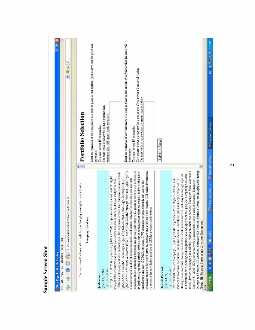
2

Sam

ple

Scre

en S

hot

12.3 Instructions for Indices

The following 5 pages are sample instructions and screenshots used in the experiment.

43

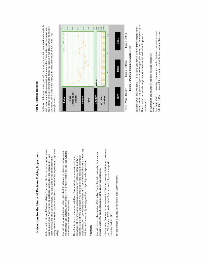
Inst

ruct

ions

for

the

Fina

ncia

l Dec

isio

n M

akin

g E

xper

imen

t W

elco

me

to th

e Fi

nanc

ial D

ecis

ion

Mak

ing

Expe

rimen

t. So

far,

you

had

a ch

ance

to lo

ok

over

the

pros

pect

us. N

ow y

ou w

ill b

e ex

plai

ned

the

deta

ils o

f the

exp

erim

ent.

If y

ou

liste

n ca

refu

lly a

nd m

ake

good

dec

isio

ns, y

ou c

ould

ear

n a

cons

ider

able

am

ount

of

mon

ey th

at w

ill b

e pa

id to

you

in c

ash

or c

heck

at t

he e

nd o

f the

exp

erim

ent (

7 da

ys fr

om

toda

y).

You

will

not

be

paire

d w

ith a

ny o

ther

indi

vidu

al. I

n ad

ditio

n, n

o ot

her p

erso

n’s d

ecis

ion

will

influ

ence

you

r out

com

e. A

ll yo

ur c

hoic

es w

ill b

e re

cord

ed to

day

and

your

out

com

e w

ill b

e re

aliz

ed o

ne w

eek

from

toda

y.

The

rule

s for

the

expe

rimen

t are

as f

ollo

ws.

Do

not t

alk

or c

omm

unic

ate

with

oth

er

parti

cipa

nts.

If y

ou a

re u

sing

a c

ompu

ter,

do n

ot u

se a

ny so

ftwar

e ot

her t

han

that

is

expl

icitl

y re

quire

d by

the

expe

rimen

t. Y

ou a

re n

ot a

llow

ed to

bro

wse

the

inte

rnet

or

chec

k em

ails

, etc

. If y

ou v

iola

te a

ny o

f the

se ru

les,

you

will

be

aske

d to

leav

e w

ithou

t pay

. Fe

el fr

ee to

ask

que

stio

ns b

y ra

isin

g yo

ur h

and

or si

gnal

ing

to th

e ex

perim

ente

r.

Paym

ent

You

will

rece

ive

a sh

ow-u

p fe

e of

$10

toda

y. Y

ou w

ill b

e to

ld in

det

ail o

f how

you

can

ar

rang

e to

pic

kup

the

addi

tiona

l ear

ning

s at t

he e

nd o

f the

exp

erim

ent.

All

acco

untin

g fr

om h

ere

on o

ut a

re d

one

in a

fict

itiou

s cur

renc

y ca

lled Francs

. Exc

hang

e ra

te: 2

00 fr

ancs

= 1

USD

. At t

he e

nd o

f the

exp

erim

ent,

all y

our e

arni

ngs w

ill b

e co

nver

ted

back

to U

SD.

The

expe

rimen

t is d

ivid

ed in

to tw

o pa

rts p

lus a

surv

ey se

ctio

n.

Part

1. P

ortfo

lio B

uild

ing

In th

is p

art o

f the

exp

erim

ent,

you

will

con

stru

ct y

our p

ortfo

lio o

ver a

serie

s of r

ound

s. In

ea

ch ro

und,

you

will

be

pres

ente

d w

ith a

stoc

k in

dex.

The

se in

dice

s are

the

indi

ces y

ou

had

a ch

ance

to lo

ok o

ver d

urin

g th

e pr

ospe

ctus

sect

ion.

You

r dec

isio

ns w

ill b

e w

heth

er

you

wan

t to

buy

a sh

are

of th

e in

dex,

sell

a sh

are

of th

e in

dex

or b

uy a

bon

d. (S

ee

exam

ple

belo

w).

Key

s: P

ress

1 fo

r Buy

.

Pre

ss 2

for B

ond.

Pre

ss 3

for S

ell.

Figu

re 1

: Por

tfolio

bui

ldin

g ex

ampl

e sc

reen

Ea

ch in

dex

will

cos

t 100

fran

cs.

To c

alcu

late

you

r pay

off f

rom

you

r inv

estm

ents

on

the

indi

ces,

we

will

pay

you

the

orig

inal

inve

stm

ent p

lus y

our p

erce

nt re

turn

mul

tiplie

d by

20.

Th

is is

don

e to

incr

ease

the

rang

e of

pos

sibl

e re

turn

s and

to si

mul

ate

long

er-te

rm

inve

stm

ents

.

To su

mm

ariz

e, th

e pa

yoff

s for

the

thre

e po

ssib

le c

hoic

es a

re:

Bon

d: 1

00

Buy

: 100

(1+2

0*r)

Y

ou b

uy if

you

wan

t to

bet t

hat t

he in

dex

valu

e w

ill in

crea

se.

Sell:

100

(1-2

0*r)

Y

ou se

ll if

you

wan

t to

bet t

hat t

he in

dex

valu

e w

ill d

ecre

ase.

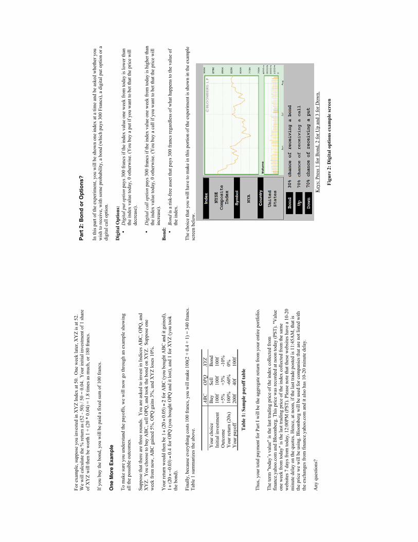
For e

xam

ple,

supp

ose

you

inve

sted

in X

YZ

Inde

x at

50.

One

wee

k la

ter,

XY

Z is

at 5

2.

We

will

cal

cula

te th

e %

retu

rn a

s (52

- 50

) / 5

0 =

0.04

. Y

our i

nitia

l inv

estm

ent o

f 1 sh

are

of X

YZ

will

then

be

wor

th 1

+ (2

0 *

0.04

) = 1

.8 ti

mes

as m

uch,

or 1

80 fr

ancs

.

If y

ou b

uy th

e bo

nd, y

ou w

ill b

e pa

id a

fixe

d su

m o

f 100

fran

cs.

On

e M

ore

Exam

ple

To

mak

e su

re y

ou u

nder

stan

d th

e pa

yoff

s, w

e w

ill n

ow g

o th

roug

h an

exa

mpl

e sh

owin

g al

l the

pos

sibl

e ou

tcom

es.

Supp

ose

that

ther

e ar

e th

ree

roun

ds.

You

are

ask

ed to

inve

st in

Indi

ces A

BC

, OPQ

, and

X

YZ.

You

cho

ose

to b

uy A

BC

, sel

l OPQ

, and

took

the

bond

on

XY

Z. S

uppo

se o

ne

wee

k fr

om n

ow, A

BC

gai

ned

5%, O

PQ g

ains

3%

, and

XY

Z lo

ses 1

0%.

Y

our r

etur

n w

ould

then

be

for A

BC

(you

bou

ght A

BC

and

it g

aine

d),

for O

PQ (y

ou b

ough

t OPQ

and

it lo

st),

and

1 fo

r XY

Z (y

ou to

ok

the

bond

).

Fina

lly, b

ecau

se e

very

thin

g co

sts 1

00 fr

ancs

, you

will

mak

e 10

0(2

+ 0.

4 +

1) =

340

fran

cs.

Tabl

e 1

sum

mar

izes

the

abov

e.

ABC

O

PQ

XYZ

You

r cho

ice

Buy

Se

ll B

ond

Initi

al in

vest

men

t 10

0f

100f

10

0f

Out

com

e +5

%

+3%

-1

0%

You

r ret

urn

(20x

) 10

0%

-60%

0%

Y

our p

ayof

f 20

0f

40f

100f

Tab

le 1

: Sam

ple

payo

ff ta

ble

Thus

, you

r tot

al p

aym

ent f

or P

art I

will

be

the

aggr

egat

e re

turn

from

you

r ent

ire p

ortfo

lio.

The

term

"to

day’

s val

ue"

is th

e la

st tr

adin

g pr

ice

of th

e in

dex

colle

cted

from

fin

ance

.yah

oo.c

om a

nd B

loom

berg

. Thi

s pric

e w

as re

cord

ed a

t noo

n to

day

(PST

). "V

alue

on

e w

eek

from

toda

y" is

the

last

trad

ing

pric

e of

the

inde

x co

llect

ed fr

om th

e sa

me

web

site

s 7 d

ays f

rom

toda

y, 1

2:00

PM (P

ST).

Plea

se n

ote

that

thes

e w

ebsi

tes h

ave

a 10

-20

min

ute

dela

y on

the

quot

es. H

ence

, at n

oon,

if th

e la

st tr

ade

post

ed is

11:

45A

M, t

hat i

s th

e pr

ice

we

will

be

usin

g. B

loom

berg

will

be

used

for c

ompa

nies

that

are

not

list

ed w

ith

the

exch

ange

s fro

m fi

nanc

e.ya

hoo.

com

and

it a

lso

has 1

0-20

min

ute

dela

y.

Any

que

stio

ns?

Part

2: B

ond

or O

ptio

ns?

In th

is p

art o

f the

exp

erim

ent,

you

will

be

show

n on

e in

dex

at a

tim

e an

d be

ask

ed w

heth

er y

ou

wis

h to

rece

ive,

with

som

e pr

obab

ility

, a b

ond

(whi

ch p

ays 3

00 F

ranc

s), a

dig

ital p

ut o

ptio

n or

a

digi

tal c

all o

ptio

n.

Dig

ital O

ptio

ns:

•

Dig

ital p

ut o

ptio

n pa

ys 3

00 fr

ancs

if th

e in

dex

valu

e on

e w

eek

from

toda

y is

low

er th

an

the

inde

x va

lue

toda

y, 0

oth

erw

ise.

(You

buy

a p

ut if

you

wan

t to

bet t

hat t

he p

rice

will

de

crea

se).

•

Dig

ital c

all o

ptio

n pa

ys 3

00 fr

ancs

if th

e in

dex

valu

e on

e w

eek

from

toda

y is

hig

her t

han

the

inde

x va

lue

toda

y, 0

oth

erw

ise.

(You

buy

a c

all i

f you

wan

t to

bet t

hat t

he p

rice

will

in

crea

se).

Bon

d:

•

Bond

is a

risk

-fre

e as

set t

hat p

ays 3

00 fr

ancs

rega

rdle

ss o

f wha

t hap

pens

to th

e va

lue

of

the

inde

x.

The

choi

ce th

at y

ou w

ill h

ave

to m

ake

in th

is p

ortio

n of

the

expe

rimen

t is s

how

n in

the

exam

ple

scre

en b

elow

.

K

eys:

Pre

ss 1

for B

ond,

2 fo

r Up

and

3 fo

r Dow

n.

Figu

re 2

: Dig

ital o

ptio

ns e

xam

ple

scre

en

As y

ou c

an se

e, y

ou a

re n

ot g

uara

ntee

d to

rece

ive

a bo

nd o

r an

optio

n. Y

ou w

ill b

e gi

ven

the

prob

abili

ty o

f rec

eivi

ng th

e ch

oice

you

sele

ct.

In th

e ab

ove

exam

ple,

if y

ou c

hoos

e to

rece

ive

a bo

nd, y

ou h

ave

30%

cha

nce

of a

ctua

lly

rece

ivin

g it.

If y

ou d

o re

ceiv

e it,

you

will

be

paid

100

fran

cs re

gard

less

of w

hat h

appe

ns to

the

valu

e of

the

inde

x. O

ther

wis

e, y

ou w

ill re

ceiv

e 0

fran

cs.

To

day'

s Ind

ex v

alue

is le

ss th

an

next

wee

k's I

ndex

Val

ue

Toda

y's I

ndex

val

ue is

gre

ater

than

nex

t w

eek'

s ind

ex v

alue

30

% c

hanc

e 30

0 Fr

ancs

30

0 Fr

ancs

70

% c

hanc

e 0

0

Tab

le 2

: Pay

off s

truc

ture

for

the

Bon

d

If y

ou c

hoos

e to

rece

ive

a pu

t opt

ion,

then

you

hav

e a

70%

cha

nce

of re

ceiv

ing

the

optio

n an

d 30

% c

hanc

e of

rece

ivin

g no

thin

g. N

ote

that

whe

n yo

u do

act

ually

rece

ive

a pu

t opt

ion,

you

are

no

t gua

rant

eed

to b

e pa

id 1

00 fr

ancs

unl

ess t

he In

dex

valu

e on

e w

eek

from

toda

y is

less

than

the

valu

e to

day.

See

the

tabl

e be

low

to g

et a

bet

ter u

nder

stan

ding

of t

he p

ayof

f.

To

day'

s Ind

ex v

alue

is le

ss th

an

next

wee

k's I

ndex

Val

ue

Toda

y's I

ndex

val

ue is

gre

ater

than

nex

t w

eek'

s ind

ex v

alue

30

% c

hanc

e 0

0 70

% c

hanc

e 0

300

fran

cs

Tab

le 3

: Pay

off s

truc

ture

for

the

Put o

ptio

n If

you

sele

ct a

Put

op

tion

Toda

y's I

ndex

val

ue is

less

than

nex

t w

eek'

s Ind

ex V

alue

To

day'

s Ind

ex v

alue

is g

reat

er th

an

next

wee

k's i

ndex

val

ue

30%

cha

nce

0 0

70%

cha

nce

300

fran

cs

0

Tab

le 4

: Pay

off s

truc

ture

for

the

Cal

l opt

ion

This

is h

ow th

e "c

hanc

e" is

det

erm

ined

in th

is se

ctio

n. If

it st

ates

that

ther

e is

a 3

0% c

hanc

e of

re

ceiv

ing

a bo

nd, i

t mea

ns th

e fo

llow

ing:

we

will

use

a ra

ndom

num

ber g

ener

ator

whi

ch g

ives

a

num

ber f

rom

1 -

100.

If th

e nu

mbe

r giv

en is

bet

wee

n 1

to 3

0 (in

clus

ive)

, you

will

rece

ive

the

bond

. Oth

erw

ise,

you

will

not

. Aga

in, i

f it s

tate

s tha

t the

re is

a 7

0% c

hanc

e of

rece

ivin

g an

op

tion,

it m

eans

the

follo

win

g: w

e w

ill u

se a

rand

om n

umbe

r gen

erat

or w

hich

giv

es a

num

ber

from

1 -

100.

If th

e nu

mbe

r is b

etw

een

31 to

100

(inc

lusi

ve),

you

will

rece

ive

the

optio

n. E

ach

of

the

trial

s is i

ndep

ende

nt o

f eac

h ot

her.

This

mea

ns th

at w

e w

ill ru

n th

e ra

ndom

num

ber g

ener

ator

ea

ch ti

me

for e

ach

trial

you

hav

e in

this

sect

ion.

Paym

ent:

You

r tot

al p

aym

ent f

rom

par

t 2 w

ill b

e ba

sed

on th

e ou

tcom

e of

eve

ry tr

ial i

n th

is

sect

ion.

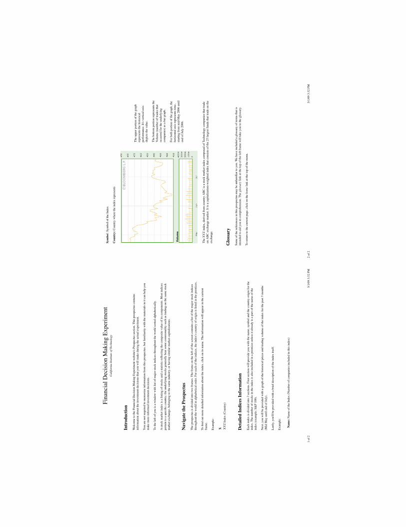
Fin

anci

al D

ecis

ion

Mak

ing

Ex

per

imen

tC

ali

forn

ia I

nst

itute

of

Tec

hnolo

gy

Intr

od

uct

ion

Wel

com

e to

the

Fin

anci

al D

ecis

ion M

akin

g E

xper

imen

t w

ebsi

te's

Pro

spec

tus

sect

ion. T

his

pro

spec

tus

conta

ins

info

rmat

ion a

bout

the

inves

tmen

t dec

isio

ns

that

you w

ill

mak

e duri

ng t

he

actu

al e

xper

imen

t.

You a

re n

ot

requir

ed t

o m

emori

ze i

nfo

rmat

ion f

rom

this

pro

spec

tus,

but

fam

ilia

rity

wit

h t

he

mat

eria

ls i

n i

t ca

n h

elp y

ou

mak

e m

ore

info

rmed

inves

tmen

t dec

isio

ns.

To t

he

left

of

you i

s a

win

dow

wit

h l

ist

of

maj

or

stock

indic

es t

hro

ughout

the

worl

d s

ort

ed a

lphab

etic

ally

.

A s

tock

mar

ket

index

is

a li

stin

g o

f st

ock

s an

d a

sta

tist

ic r

eec

ting t

he

com

posi

te v

alue

of

its

com

ponen

ts. M

ost

indic

es

per

tain

to a

spec

ic

countr

y;

the

under

lyin

g s

tock

s gen

eral

ly b

ear

som

e co

mm

onal

ity s

uch

as

trad

ing o

n t

he

sam

e st

ock

mar

ket

exch

ange,

bel

ongin

g t

o t

he

sam

e in

dust

ry, or

hav

ing s

imil

ar m

arket

cap

ital

izat

ions.

Navig

ate

th

e P

rosp

ectu

s

The

pro

spec

tus

is d

ivid

ed i

nto

tw

o f

ram

es. T

he

fram

e on t

he

left

of

the

scre

en c

onta

ins

a li

st o

f th

e m

ajor

stock

indic

es

thro

ughout

the

worl

d i

n a

lphab

etic

al o

rder

. F

or

each

of

the

indic

es, th

e in

dex

's c

ountr

y o

f ori

gin

is

list

ed i

n t

he

pre

nti

ces.

To

nd o

ut

more

det

aile

d i

nfo

rmat

ion a

bout

the

index

, cl

ick o

n i

ts n

ame.

The

info

rmat

ion w

ill

appea

r in

the

curr

ent

fram

e.

Exam

ple

:

X XY

Z I

ndex

(C

ountr

y)

Deta

iled

In

dic

es I

nfo

rm

ati

on

Eac

h i

ndex

is

div

ided

into

3 s

ecti

ons.

Fir

st s

ecti

on w

ill

pro

vid

e you w

ith t

he

nam

e, s

ym

bol

and t

he

countr

y o

rigin

for

the

index

. T

he

num

ber

of

stock

s in

the

index

is

also

incl

uded

in a

pre

nti

ces

unle

ss i

t al

read

y i

s a

par

t of

the

nam

e of

the

index

(ex

ample

: S

&P

100).

Nex

t, y

ou w

ill

be

pro

vid

ed w

ith a

gra

ph o

f th

e his

tori

cal

pri

ces

and t

radin

g v

olu

me

of

the

index

for

the

pas

t 3 m

onth

s

(Mid

May

unti

l en

d o

f Ju

ly).

Las

tly,

you'll

be

pro

vid

ed w

ith a

bri

ef d

escr

ipti

on o

f th

e in

dex

its

elf.

Exam

ple

:

Name:

Nam

e of

the

Index

(N

um

ber

of

com

pan

ies

incl

uded

in t

his

index

)

1 o

f 2

5/1

/09 3

:32 P

M

Sym

bo

l: S

ym

bol

of

the

Index

Cou

ntr

y:

Countr

y w

her

e th

e in

dex

rep

rese

nts

The

upper

port

ion o

f th

e gra

ph

repre

sents

the

his

tori

cal

per

form

ance

. It

's v

erti

cal

axis

dep

icts

the

val

ue.

The

bott

om

port

ion r

epre

sents

the

Volu

me

(num

ber

of

trad

es t

hat

occ

urr

ed f

or

the

under

lyin

g

com

pan

ies)

as

a bar

gra

ph.

For

both

port

ion o

f th

e gra

ph, th

e

hori

zonta

l ax

is r

epre

sents

tim

e,

star

ting f

rom

mid

-May

2006 u

nti

l

end o

f Ju

ly 2

006.

The

XY

Z in

dex,

der

ived

from

cou

ntry

AB

C is

a st

ock

mar

ket i

ndex

com

pose

d of

Tec

hnol

ogy

com

pani

es th

at tr

ade

on A

BC

exc

hang

e m

arke

t. It

is a

cap

italiz

atio

n-w

eigh

ted

inde

x th

at c

onsi

sts o

f the

25

larg

est f

unds

that

trad

e on

the

exch

ange

.

Glossary

Som

e of

the

refe

rence

s in

this

pro

spec

tus

may

be

unfa

mil

iar

to y

ou. W

e hav

e in

cluded

a g

loss

ary o

f te

rms

that

is

inte

nded

to a

id y

ou i

n c

om

pre

hen

sion. T

he

glo

ssary

lin

k a

t th

e to

p o

f th

e le

ft f

ram

e w

ill

take

you t

o t

he

glo

ssar

y.

To r

eturn

to t

he

curr

ent

pag

e, c

lick

on t

he

hom

e li

nk a

t th

e to

p o

f th

e m

enu.

2 o

f 2

5/1

/09 3

:32 P

M

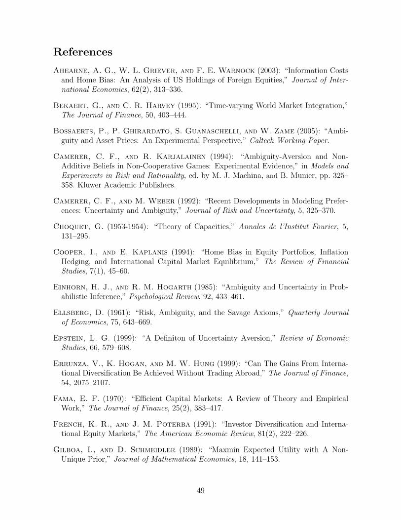
References

Ahearne, A. G., W. L. Griever, and F. E. Warnock (2003): “Information Costsand Home Bias: An Analysis of US Holdings of Foreign Equities,” Journal of Inter-national Economics, 62(2), 313–336.

Bekaert, G., and C. R. Harvey (1995): “Time-varying World Market Integration,”The Journal of Finance, 50, 403–444.

Bossaerts, P., P. Ghirardato, S. Guanaschelli, and W. Zame (2005): “Ambi-guity and Asset Prices: An Experimental Perspective,” Caltech Working Paper.

Camerer, C. F., and R. Karjalainen (1994): “Ambiguity-Aversion and Non-Additive Beliefs in Non-Cooperative Games: Experimental Evidence,” in Models andExperiments in Risk and Rationality, ed. by M. J. Machina, and B. Munier, pp. 325–358. Kluwer Academic Publishers.

Camerer, C. F., and M. Weber (1992): “Recent Developments in Modeling Prefer-ences: Uncertainty and Ambiguity,” Journal of Risk and Uncertainty, 5, 325–370.

Choquet, G. (1953-1954): “Theory of Capacities,” Annales de l’Institut Fourier, 5,131–295.

Cooper, I., and E. Kaplanis (1994): “Home Bias in Equity Portfolios, InflationHedging, and International Capital Market Equilibrium,” The Review of FinancialStudies, 7(1), 45–60.

Einhorn, H. J., and R. M. Hogarth (1985): “Ambiguity and Uncertainty in Prob-abilistic Inference,” Psychological Review, 92, 433–461.

Ellsberg, D. (1961): “Risk, Ambiguity, and the Savage Axioms,” Quarterly Journalof Economics, 75, 643–669.

Epstein, L. G. (1999): “A Definiton of Uncertainty Aversion,” Review of EconomicStudies, 66, 579–608.

Errunza, V., K. Hogan, and M. W. Hung (1999): “Can The Gains From Interna-tional Diversification Be Achieved Without Trading Abroad,” The Journal of Finance,54, 2075–2107.

Fama, E. F. (1970): “Efficient Capital Markets: A Review of Theory and EmpiricalWork,” The Journal of Finance, 25(2), 383–417.

French, K. R., and J. M. Poterba (1991): “Investor Diversification and Interna-tional Equity Markets,” The American Economic Review, 81(2), 222–226.

Gilboa, I., and D. Schmeidler (1989): “Maxmin Expected Utility with A Non-Unique Prior,” Journal of Mathematical Economics, 18, 141–153.

49

Glassman, D. A., and L. A. Riddick (2001): “What Causes Home Asset Bias andHow Should It be Measured?,” Journal of Empirical Finance, 8(1), 35–54.

Karolyi, G. A., and R. M. Stulz (2003): “Are Financial Assets Priced Locally orGlobally?,” in Handbook of the Economics of Finance, ed. by G. M. Constantinides,M. Harris, and R. M. Stulz, vol. 1, pp. 975–1014. Elsevier North Holland.

Kilka, M., and M. Weber (2002): “Home Bias in International Stock Return Expec-tations,” The Journal of Psychology and Financial Markets, pp. 176–192.

Knight, F. (1921): Risk, Uncertainty and Profit. Houghton Mifflin.

Lewis, K. K. (1999): “Trying to Explain Home Bias in Equities and Consumption,”Journal of Economic Literature, XXXVII, 571–608.

Nieuwerburgh, S. V., and L. Veldkamp (Forthcoming 2008): “Information Immo-bility and the Home Bias Puzzle,” The Journal of Finance.

Sarin, R., and R. L. Winkler (1992): “Ambiguity and Decision MOdeling: APreference-based Approach,” Journal of Risk and Uncertainty, 5, 389–407.

Savage, L. J. (1954): The Foundations of Statistics. Wiley.

Schmeidler, D. (1989): “Subjective Probability and Expected Utility Without Addi-tivity,” Econometrica, 57, 571–587.

Segal, U. (1987): “The Ellsberg Paradox and Risk-Aversion: An Anticipated UtilityApproach,” International Economic Review, 28, 175–202.

Smith, V. L. (1969): “Measuring Nonmonetary Utilities in Uncertain Choices: TheEllsberg Urn,” Quarterly Journal of Economics, 83, 324–329.

50