Diving into scientific PythonTraining SessionEuroPython 2011

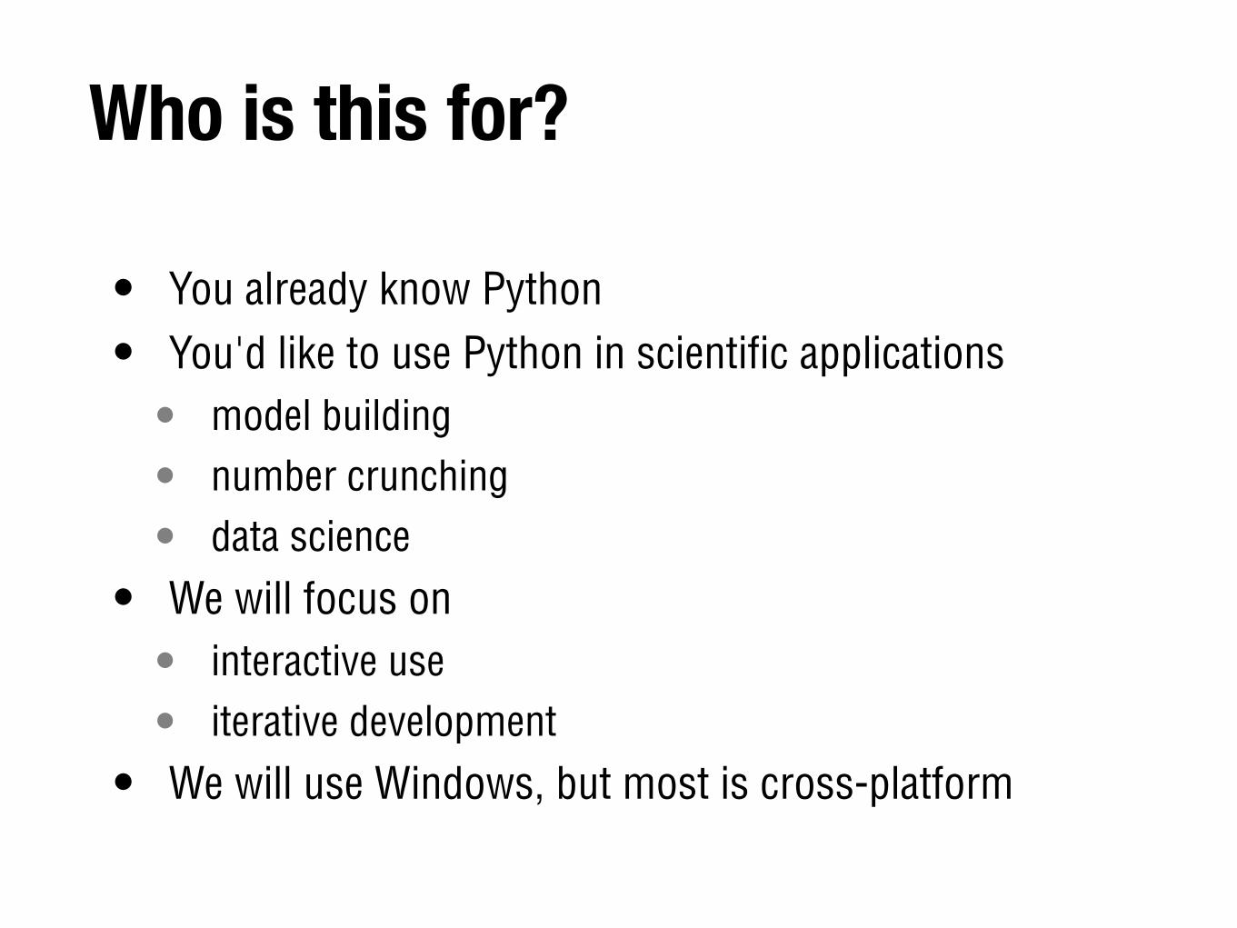
Who is this for?

• You already know Python

• You'd like to use Python in scientific applications• model building

• number crunching

• data science

• We will focus on• interactive use

• iterative development

• We will use Windows, but most is cross-platform

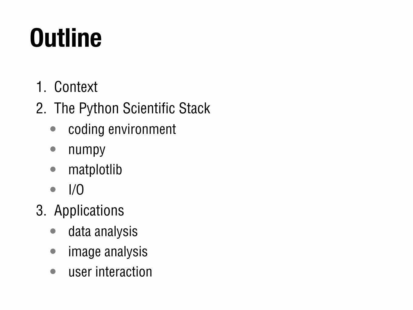
Outline1. Context 2. The Python Scientific Stack

• coding environment

• numpy

• matplotlib

• I/O3. Applications

• data analysis

• image analysis

• user interaction

1. Context

As you know by now, Python is...

• a general-purpose language

• easy to write, read and maintain (generally)

• interpreted - no compilation

• garbage-collected - no memory management

• weakly typed (duck typing)

• object-oriented if you want it to

• cross-platform: Linux, Mac OS X, Windows

Science & Engineering

• Python has been around for a while in scientific and engineering communities• "glue" language

• During the past 10 years, Python became a viable end solution for scientific computing, data analysis, plotting...

• This is mostly thanks to lots of efforts from the Open Source community, leading to the availability of mature 3rd-party toolse.g. numpy, scipy, matplotlib, ipython...

• Lots of momentum right now

Fragmentation

• Problem

• fast Python development = lots of different versions

• lots of packages to install, each with lots of versions and dependencies on each other

• to install the whole stack can be tricky

• even linux distros sometimes don't get it right

• Solution: Python distributions

• Everything is in the box

• stabilized

Python distributions

strong points weakness

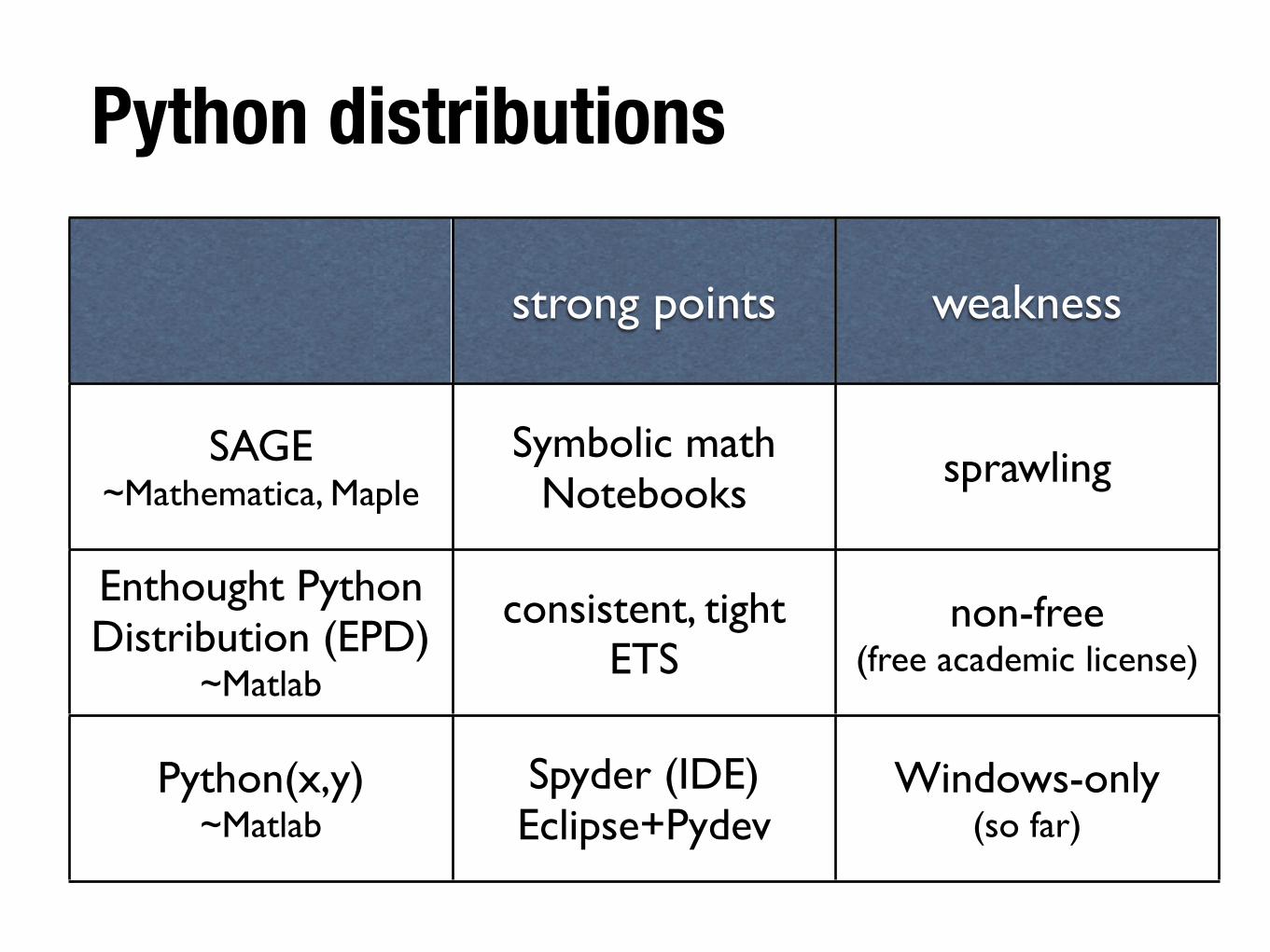
SAGE~Mathematica, Maple

Symbolic mathNotebooks

sprawling

Enthought Python Distribution (EPD)

~Matlab

consistent, tightETS

non-free(free academic license)

Python(x,y)~Matlab

Spyder (IDE)Eclipse+Pydev

Windows-only(so far)

Python(x,y)

• http://www.pythonxy.org

• Provides• A recent version of Python (2.6.6, 2.7 soon)

• lots of packages and modules for engineering in Python, all pre-configured

• Visualization tools

• improved consoles

• Spyder (Matlab-like IDE)

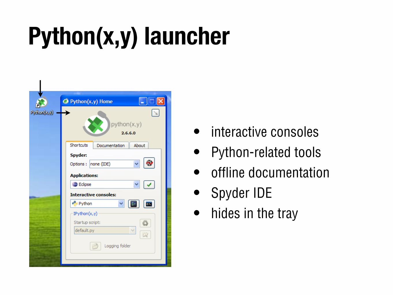
Python(x,y) launcher

• interactive consoles

• Python-related tools

• offline documentation

• Spyder IDE

• hides in the tray

Note

• Most scientific modules not ready (yet) for Python >= 3.0

• Porting of numpy/matplotlib underway

• Stick to 2.6/2.7 for now

2. The Python Scientific Stack

2. The Python Scientific Stack

1. Coding Environment

Spyder

• Spyder: programming environment• file explorer

• code editor with autocompletion, suggestions

• improved IPython console

• contextual help linked to code editor, console

• variable explorer (editable)

• continuous code analysis

Spyder

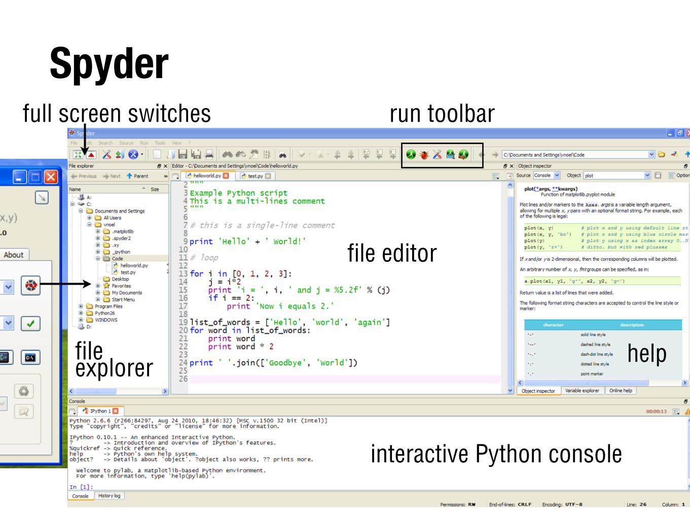
file editor

help

interactive Python console

file explorer

run toolbarfull screen switches

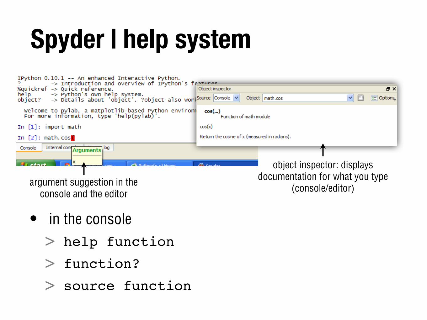
Spyder | help system

argument suggestion in the console and the editor

object inspector: displays documentation for what you type

(console/editor)

• in the console> help function

> function?

> source function

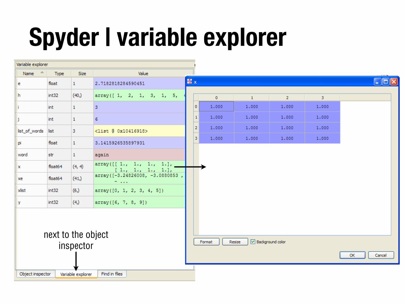
Spyder | variable explorer

next to the object inspector

IPython

• In Spyder, the default Python console is IPython• much better than the standard Python console

• tab completion for functions, modules, variables, files

• filesystem navigation (cd, ls, pwd)

• syntax highlighting

• works fine with matplotlib

IPython

• "magic" commands• %command

• type %⇥ to see them all

• (you can drop the % for most of commands)

> whos

> reset

> run script.py

> timeit y = cos(x)

IPython

• The output of the nth command is in _n

• In [183]: exp(-pi)Out[183]: 0.043213918263772258

• In [184]: _183 * 2Out[184]: 0.086427836527544516

Projects

• Spyder, IPython• interactive use

• data exploration

• iterative development of models and workflows

• Project-oriented development (i.e. full applications): Python(x,y) includes Eclipse and Pydev• we won't cover that today

2. The Python Scientific Stack

2. Numpy

numpy

• Numpy provides the array variable • n-dimensional, typed

> from numpy import array

• and related functions

• developed since 1995• child of Numeric and numarray

• now stable and mature, v.1.6 released May 2011

• Python 3 coming up

• basis for scipy, matplotlib, and lots of others

numpy | importing

• IPython imports all numpy automatically> from numpy import *

• Numpy functions can be called without prefix

• convenient for interactive use

• In scripts, import numpy as np is better

• Official convention (examples, etc.)

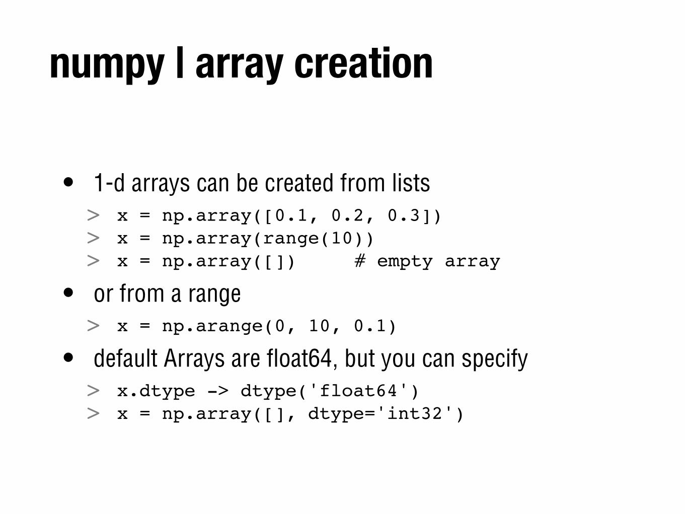
numpy | array creation

• 1-d arrays can be created from lists> x = np.array([0.1, 0.2, 0.3])> x = np.array(range(10))> x = np.array([])! ! # empty array!

• or from a range> x = np.arange(0, 10, 0.1)

• default Arrays are float64, but you can specify> x.dtype -> dtype('float64')> x = np.array([], dtype='int32')

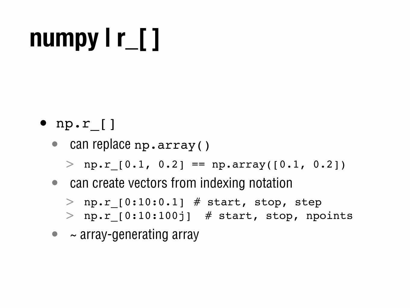
numpy | r_[ ]

• np.r_[]

• can replace np.array()> np.r_[0.1, 0.2] == np.array([0.1, 0.2])

• can create vectors from indexing notation> np.r_[0:10:0.1]! # start, stop, step> np.r_[0:10:100j] # start, stop, npoints

• ~ array-generating array

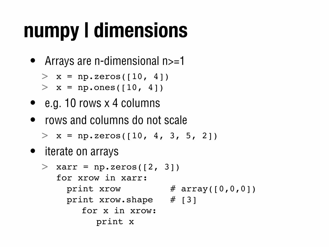
numpy | dimensions• Arrays are n-dimensional n>=1> x = np.zeros([10, 4])!> x = np.ones([10, 4])

• e.g. 10 rows x 4 columns

• rows and columns do not scale> x = np.zeros([10, 4, 3, 5, 2])

• iterate on arrays> xarr = np.zeros([2, 3])

for xrow in xarr:! print xrow!! ! ! # array([0,0,0])! print xrow.shape!! # [3]! ! for x in xrow:! ! ! print x

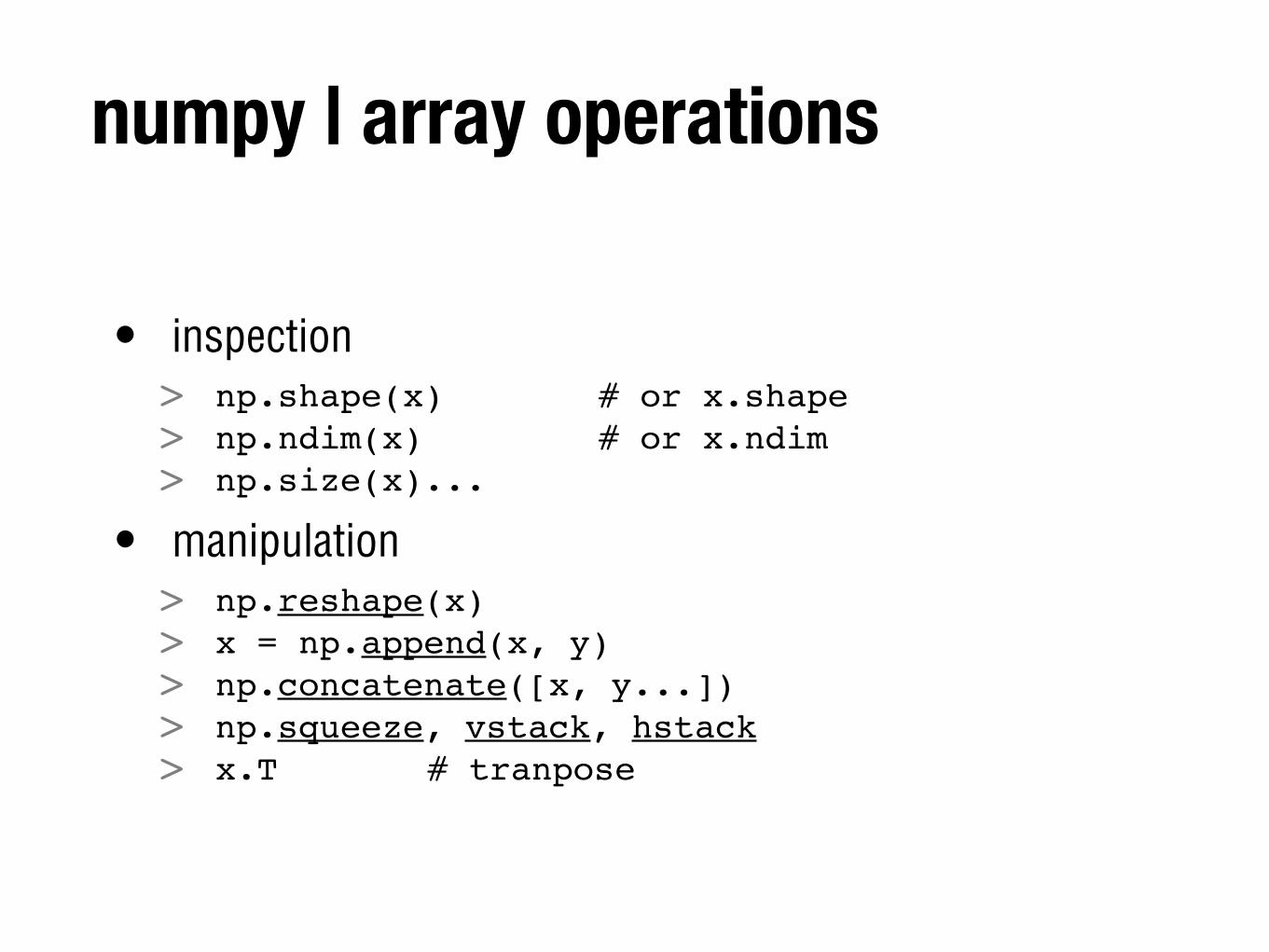
numpy | array operations

• inspection> np.shape(x) !! ! # or x.shape> np.ndim(x)!! ! ! # or x.ndim> np.size(x)...

• manipulation> np.reshape(x)> x = np.append(x, y)> np.concatenate([x, y...])> np.squeeze, vstack, hstack> x.T! ! ! # tranpose

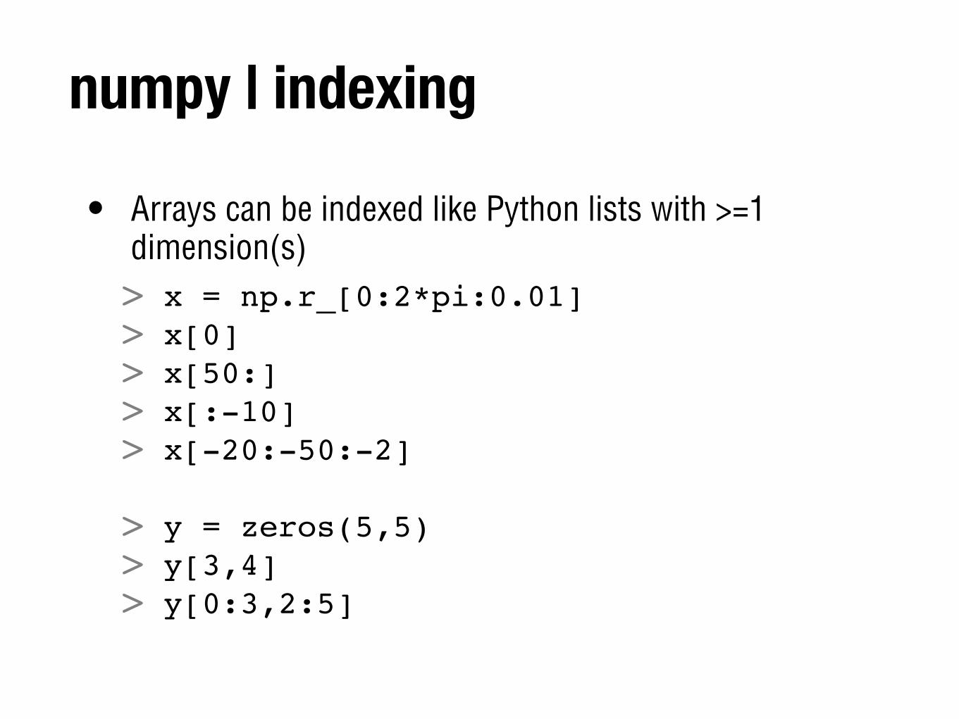
numpy | indexing

• Arrays can be indexed like Python lists with >=1 dimension(s)> x = np.r_[0:2*pi:0.01]> x[0]> x[50:]> x[:-10]> x[-20:-50:-2]

> y = zeros(5,5)> y[3,4]> y[0:3,2:5]

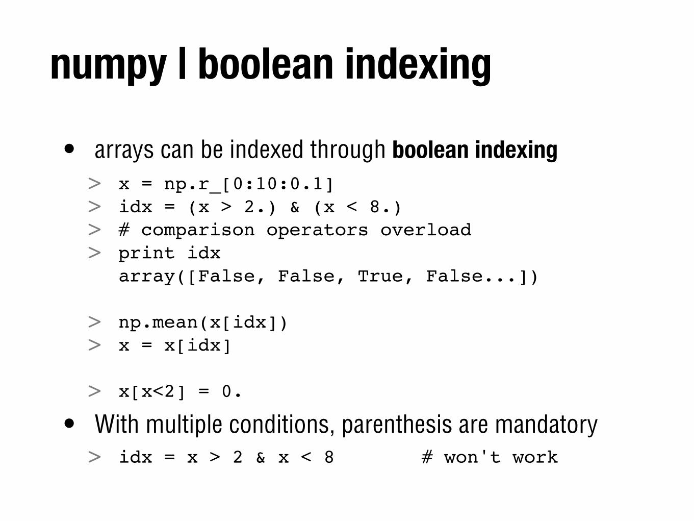
numpy | boolean indexing

• arrays can be indexed through boolean indexing> x = np.r_[0:10:0.1]> idx = (x > 2.) & (x < 8.)> # comparison operators overload> print idx

array([False, False, True, False...])

> np.mean(x[idx])> x = x[idx]

> x[x<2] = 0.

• With multiple conditions, parenthesis are mandatory> idx = x > 2 & x < 8! ! ! # won't work

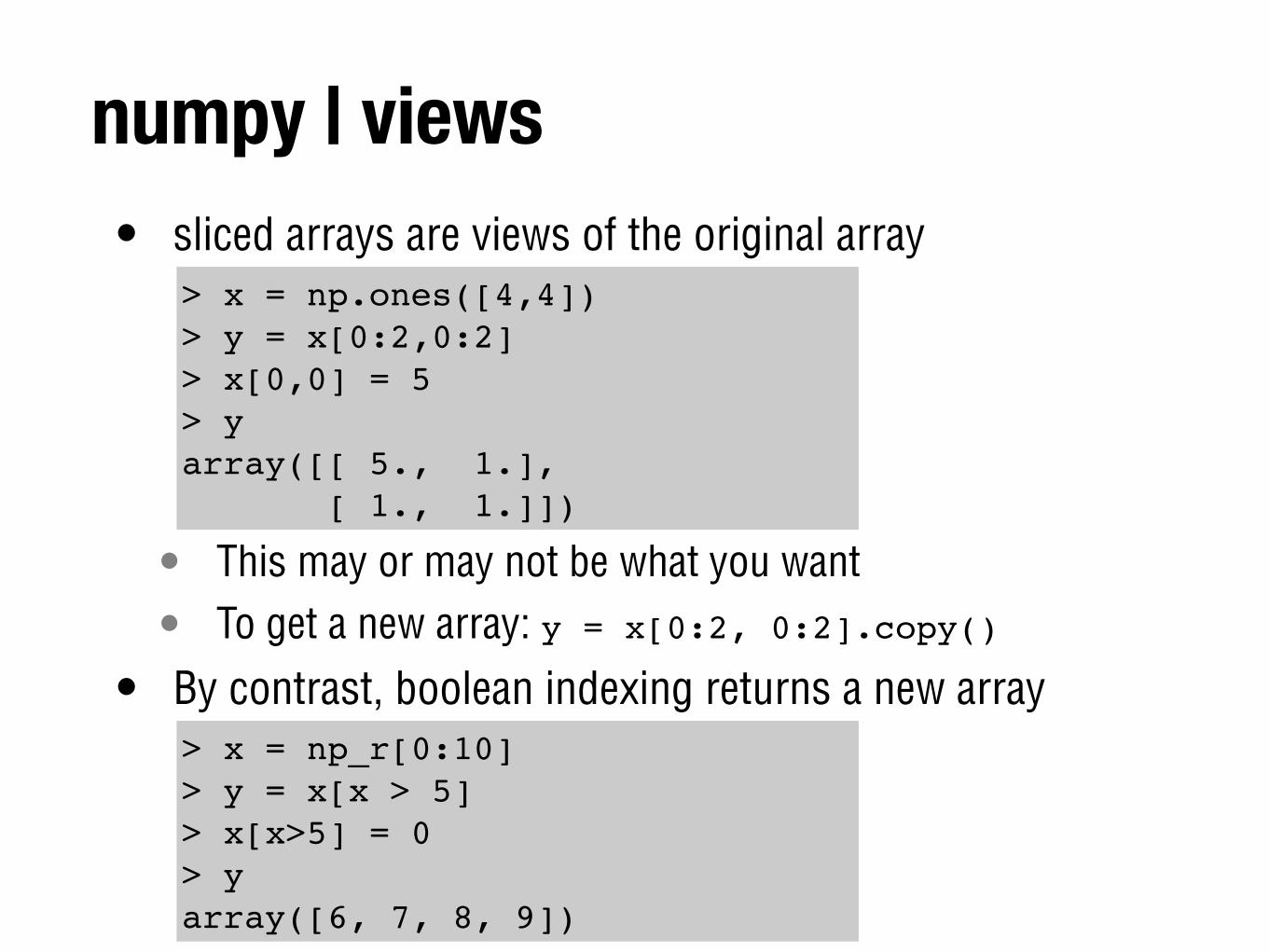
numpy | views• sliced arrays are views of the original array

• This may or may not be what you want

• To get a new array: y = x[0:2, 0:2].copy()

• By contrast, boolean indexing returns a new array

> x = np.ones([4,4])> y = x[0:2,0:2]> x[0,0] = 5> yarray([[ 5., 1.], [ 1., 1.]])

> x = np_r[0:10]> y = x[x > 5]> x[x>5] = 0> yarray([6, 7, 8, 9])

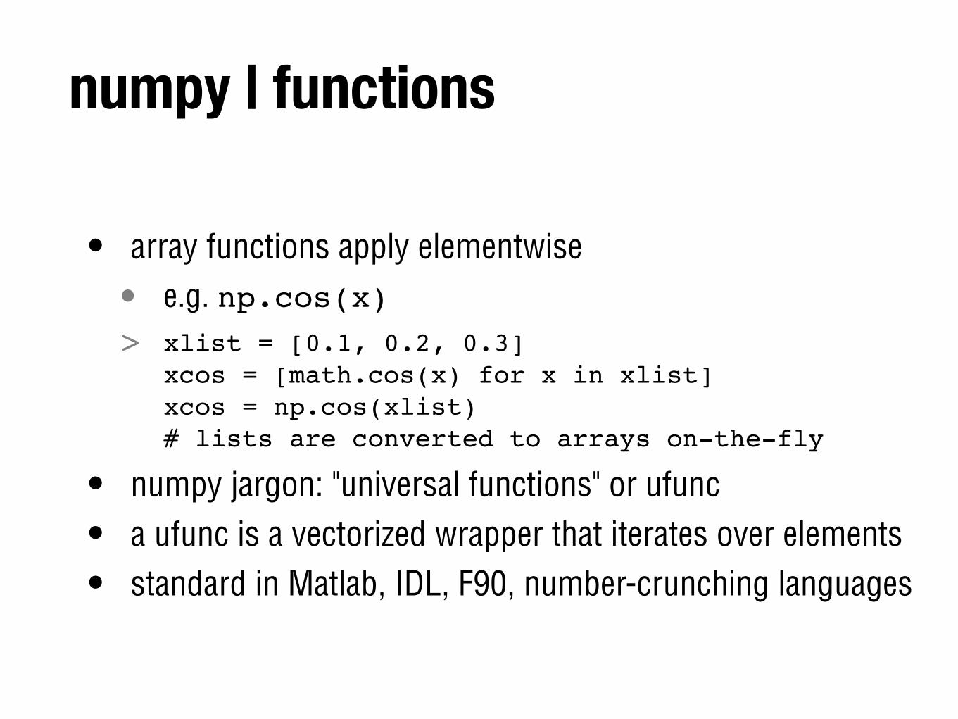
numpy | functions

• array functions apply elementwise

• e.g. np.cos(x)> xlist = [0.1, 0.2, 0.3]

xcos = [math.cos(x) for x in xlist]xcos = np.cos(xlist)# lists are converted to arrays on-the-fly

• numpy jargon: "universal functions" or ufunc

• a ufunc is a vectorized wrapper that iterates over elements

• standard in Matlab, IDL, F90, number-crunching languages

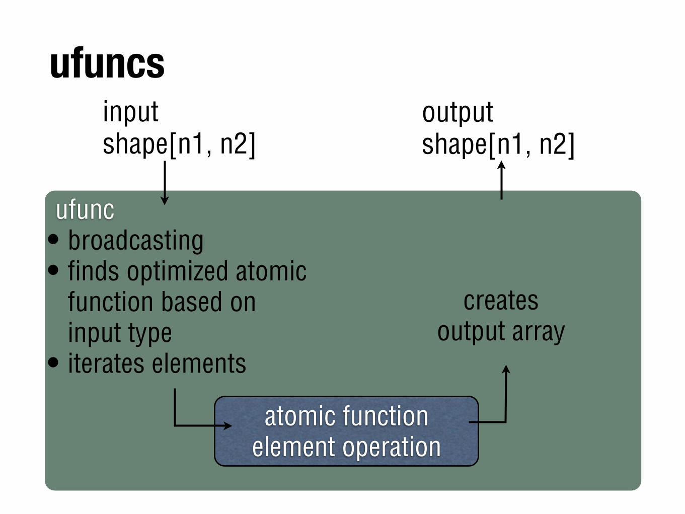
ufuncs

ufunc• broadcasting• finds optimized atomic

function based on input type

• iterates elements

inputshape[n1, n2]

outputshape[n1, n2]

atomic functionelement operation

creates output array

numpy | functions

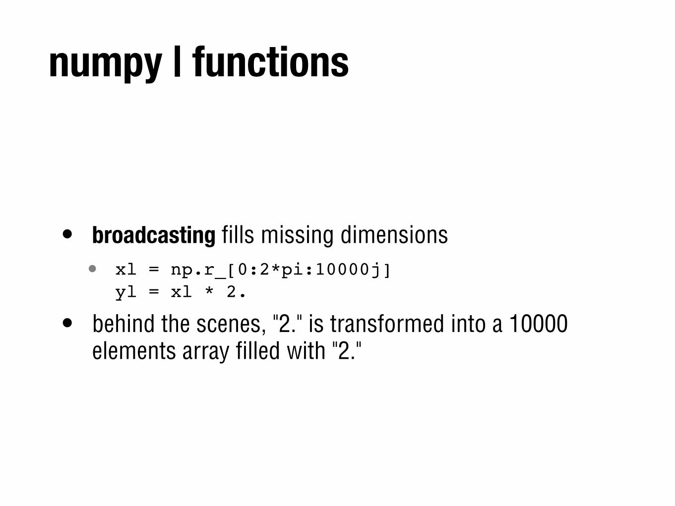
• broadcasting fills missing dimensions• xl = np.r_[0:2*pi:10000j]

yl = xl * 2.

• behind the scenes, "2." is transformed into a 10000 elements array filled with "2."

numpy | functions

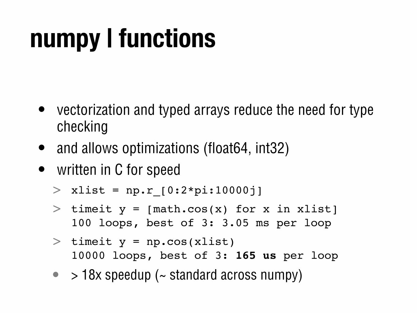
• vectorization and typed arrays reduce the need for type checking

• and allows optimizations (float64, int32)

• written in C for speed> xlist = np.r_[0:2*pi:10000j]

> timeit y = [math.cos(x) for x in xlist]100 loops, best of 3: 3.05 ms per loop

> timeit y = np.cos(xlist)10000 loops, best of 3: 165 us per loop

• > 18x speedup (~ standard across numpy)

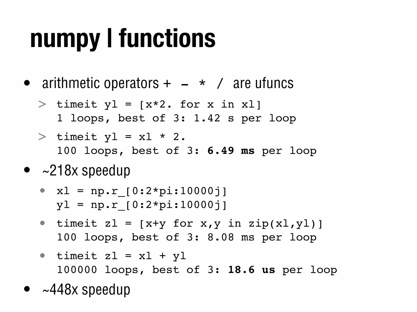
numpy | functions• arithmetic operators + - * / are ufuncs> timeit yl = [x*2. for x in xl]

1 loops, best of 3: 1.42 s per loop

> timeit yl = xl * 2.100 loops, best of 3: 6.49 ms per loop

• ~218x speedup• xl = np.r_[0:2*pi:10000j]

yl = np.r_[0:2*pi:10000j]

• timeit zl = [x+y for x,y in zip(xl,yl)]100 loops, best of 3: 8.08 ms per loop

• timeit zl = xl + yl100000 loops, best of 3: 18.6 us per loop

• ~448x speedup

numpy | functions

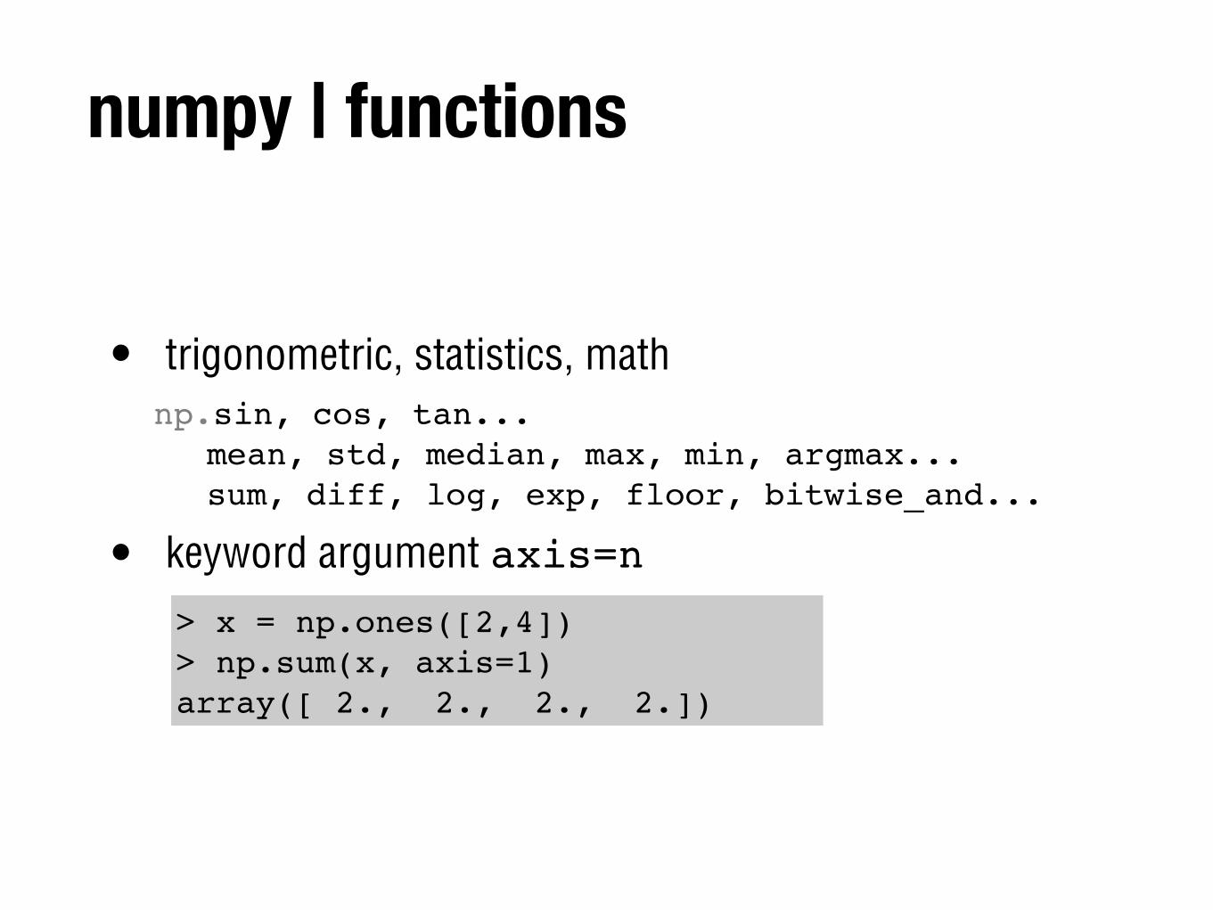
• trigonometric, statistics, mathnp.sin, cos, tan...

mean, std, median, max, min, argmax...sum, diff, log, exp, floor, bitwise_and...

• keyword argument axis=n> x = np.ones([2,4])> np.sum(x, axis=1)array([ 2., 2., 2., 2.])

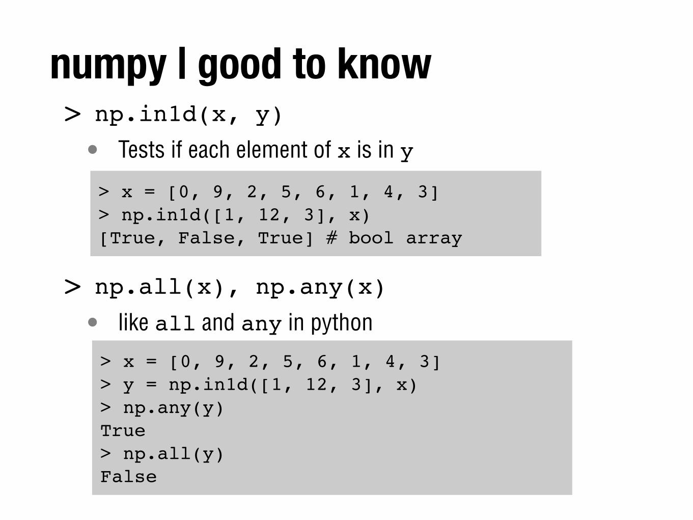
numpy | good to know> np.in1d(x, y)

• Tests if each element of x is in y

> np.all(x), np.any(x)

• like all and any in python

> x = [0, 9, 2, 5, 6, 1, 4, 3]> np.in1d([1, 12, 3], x)[True, False, True] # bool array

> x = [0, 9, 2, 5, 6, 1, 4, 3]> y = np.in1d([1, 12, 3], x)> np.any(y)True> np.all(y)False

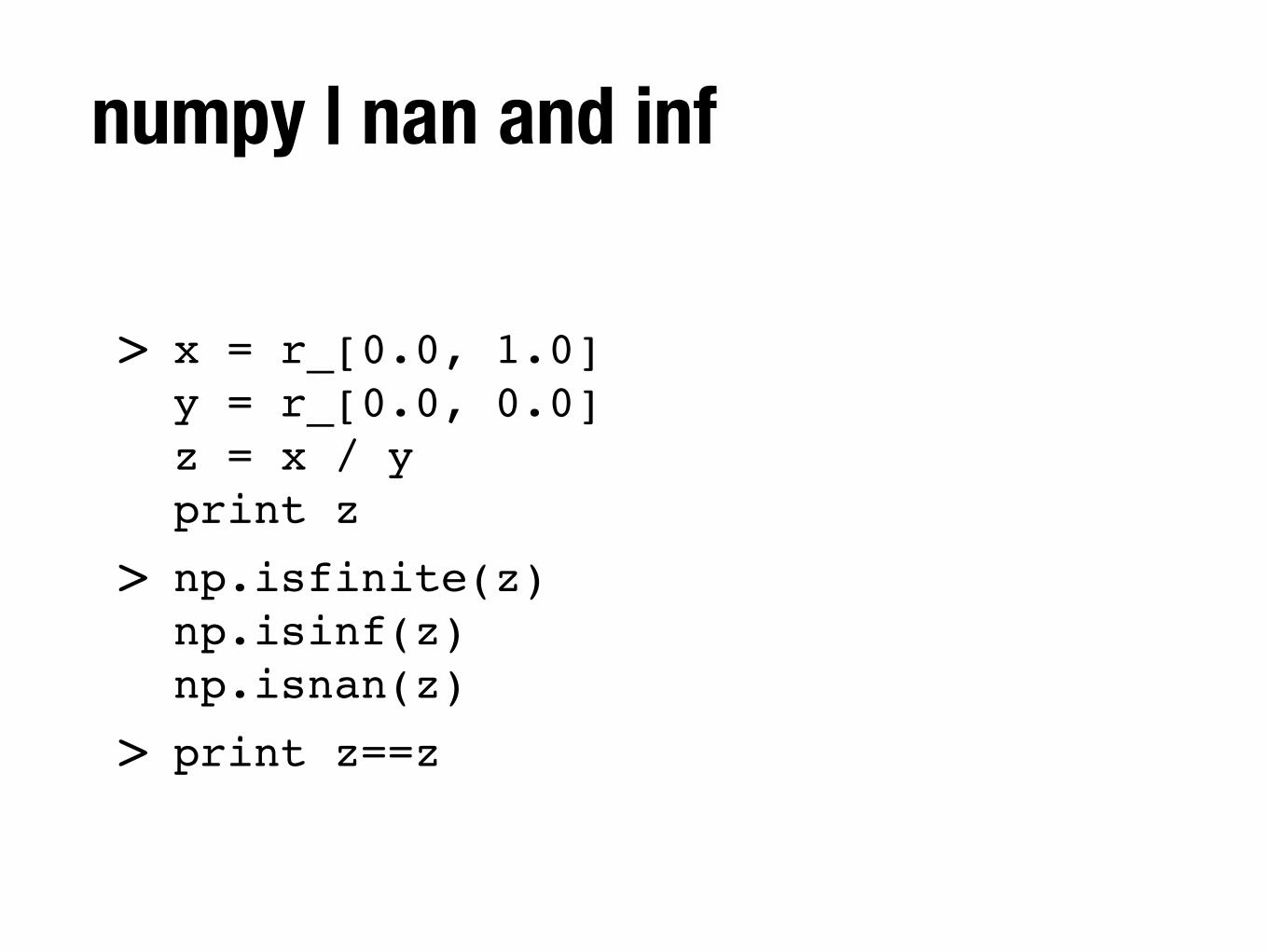
numpy | nan and inf

> x = r_[0.0, 1.0]y = r_[0.0, 0.0]z = x / yprint z

> np.isfinite(z)np.isinf(z)np.isnan(z)

> print z==z

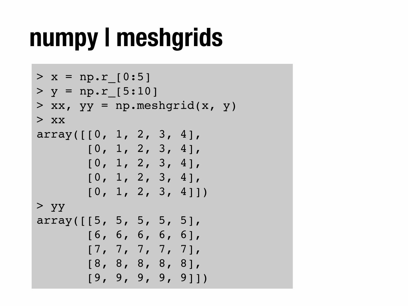
numpy | meshgrids> x = np.r_[0:5]> y = np.r_[5:10]> xx, yy = np.meshgrid(x, y)> xxarray([[0, 1, 2, 3, 4], [0, 1, 2, 3, 4], [0, 1, 2, 3, 4], [0, 1, 2, 3, 4], [0, 1, 2, 3, 4]])> yyarray([[5, 5, 5, 5, 5], [6, 6, 6, 6, 6], [7, 7, 7, 7, 7], [8, 8, 8, 8, 8], [9, 9, 9, 9, 9]])

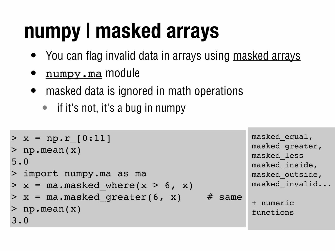
numpy | masked arrays• You can flag invalid data in arrays using masked arrays

• numpy.ma module

• masked data is ignored in math operations• if it's not, it's a bug in numpy

> x = np.r_[0:11]> np.mean(x)5.0> import numpy.ma as ma> x = ma.masked_where(x > 6, x)> x = ma.masked_greater(6, x)! ! # same> np.mean(x)3.0

masked_equal, masked_greater, masked_lessmasked_inside, masked_outside,masked_invalid...

+ numeric functions

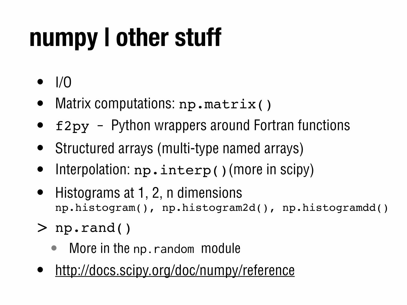
numpy | other stuff• I/O

• Matrix computations: np.matrix()

• f2py - Python wrappers around Fortran functions

• Structured arrays (multi-type named arrays)

• Interpolation: np.interp() (more in scipy)

• Histograms at 1, 2, n dimensionsnp.histogram(), np.histogram2d(), np.histogramdd()

> np.rand()

• More in the np.random module

• http://docs.scipy.org/doc/numpy/reference

2. The Python Scientific Stack

3. Matplotlib

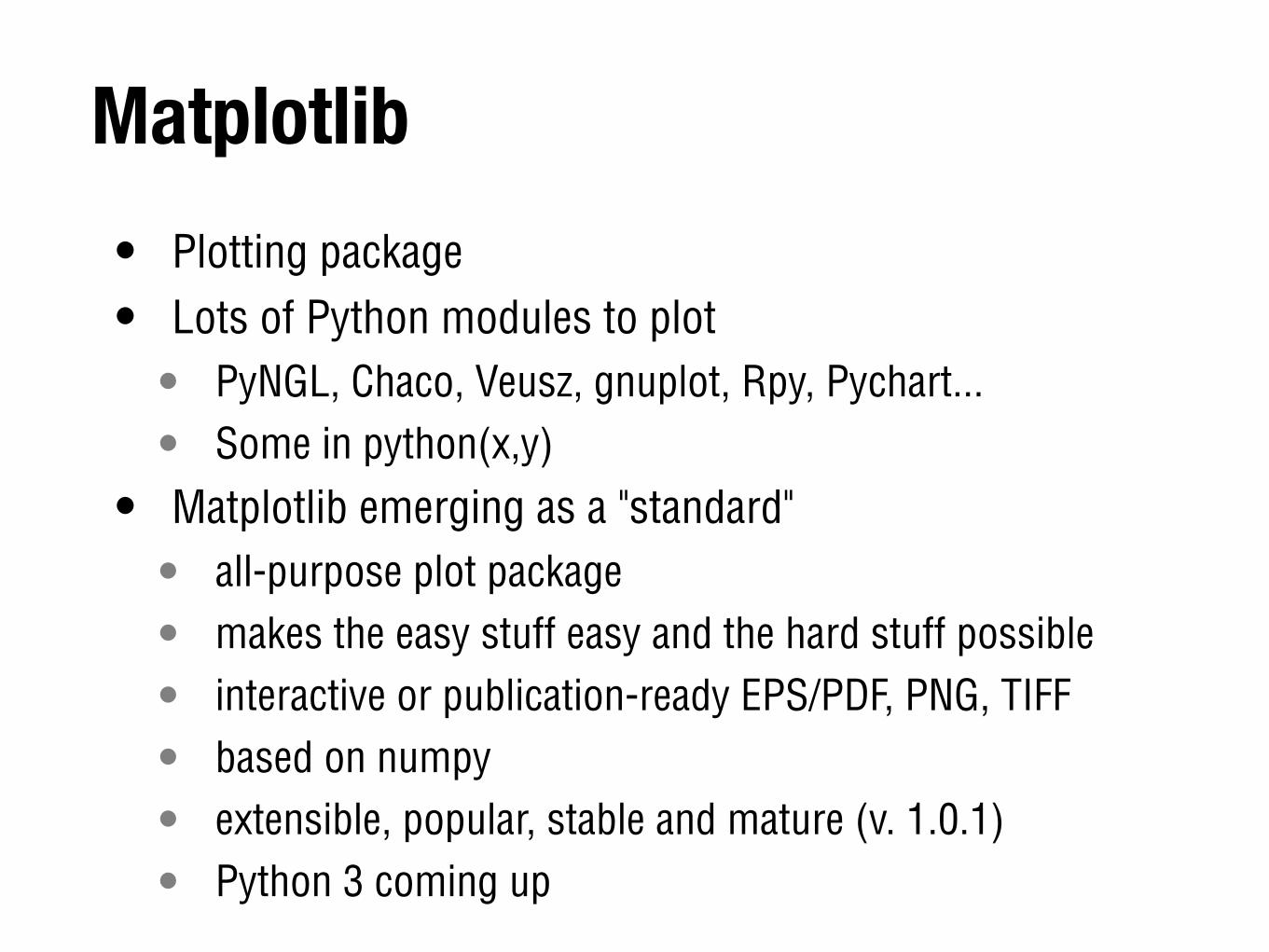
Matplotlib• Plotting package

• Lots of Python modules to plot• PyNGL, Chaco, Veusz, gnuplot, Rpy, Pychart...

• Some in python(x,y)

• Matplotlib emerging as a "standard"• all-purpose plot package

• makes the easy stuff easy and the hard stuff possible

• interactive or publication-ready EPS/PDF, PNG, TIFF

• based on numpy

• extensible, popular, stable and mature (v. 1.0.1)

• Python 3 coming up

Matplotlib & Matlab

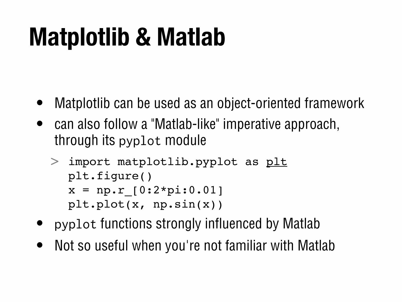
• Matplotlib can be used as an object-oriented framework

• can also follow a "Matlab-like" imperative approach, through its pyplot module> import matplotlib.pyplot as plt

plt.figure()x = np.r_[0:2*pi:0.01]plt.plot(x, np.sin(x))

• pyplot functions strongly influenced by Matlab

• Not so useful when you're not familiar with Matlab

Matplotlib in python(x,y)

• IPython imports all matplotlib.pyplot

• You can drop the plt. prefix during interactive use

• help plotting

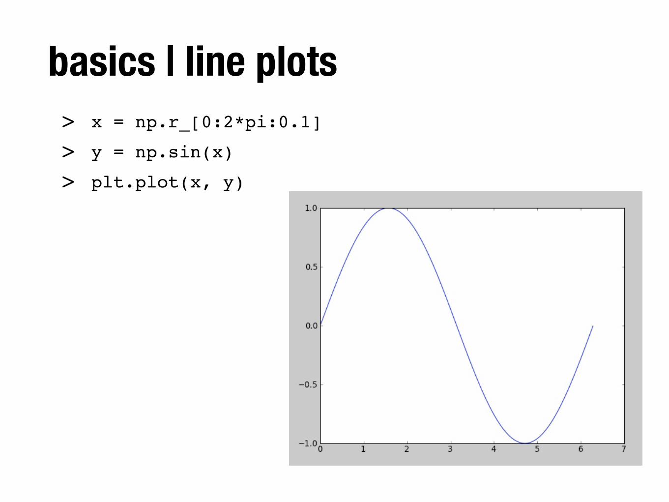
basics | line plots> x = np.r_[0:2*pi:0.1]

> y = np.sin(x)

> plt.plot(x, y)

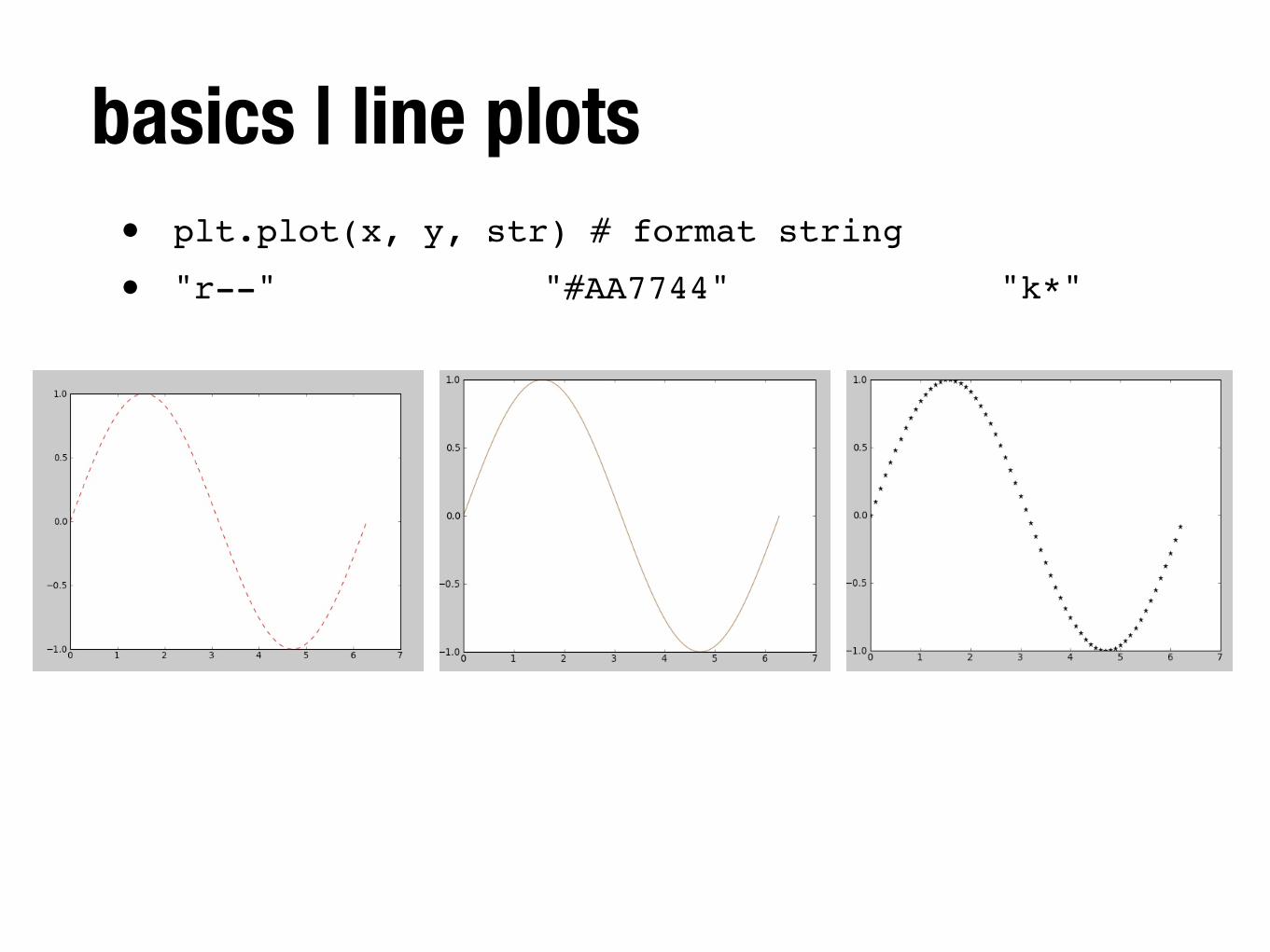
basics | line plots• plt.plot(x, y, str) # format string

• "r--"! ! ! ! ! "#AA7744"! ! ! ! ! "k*"

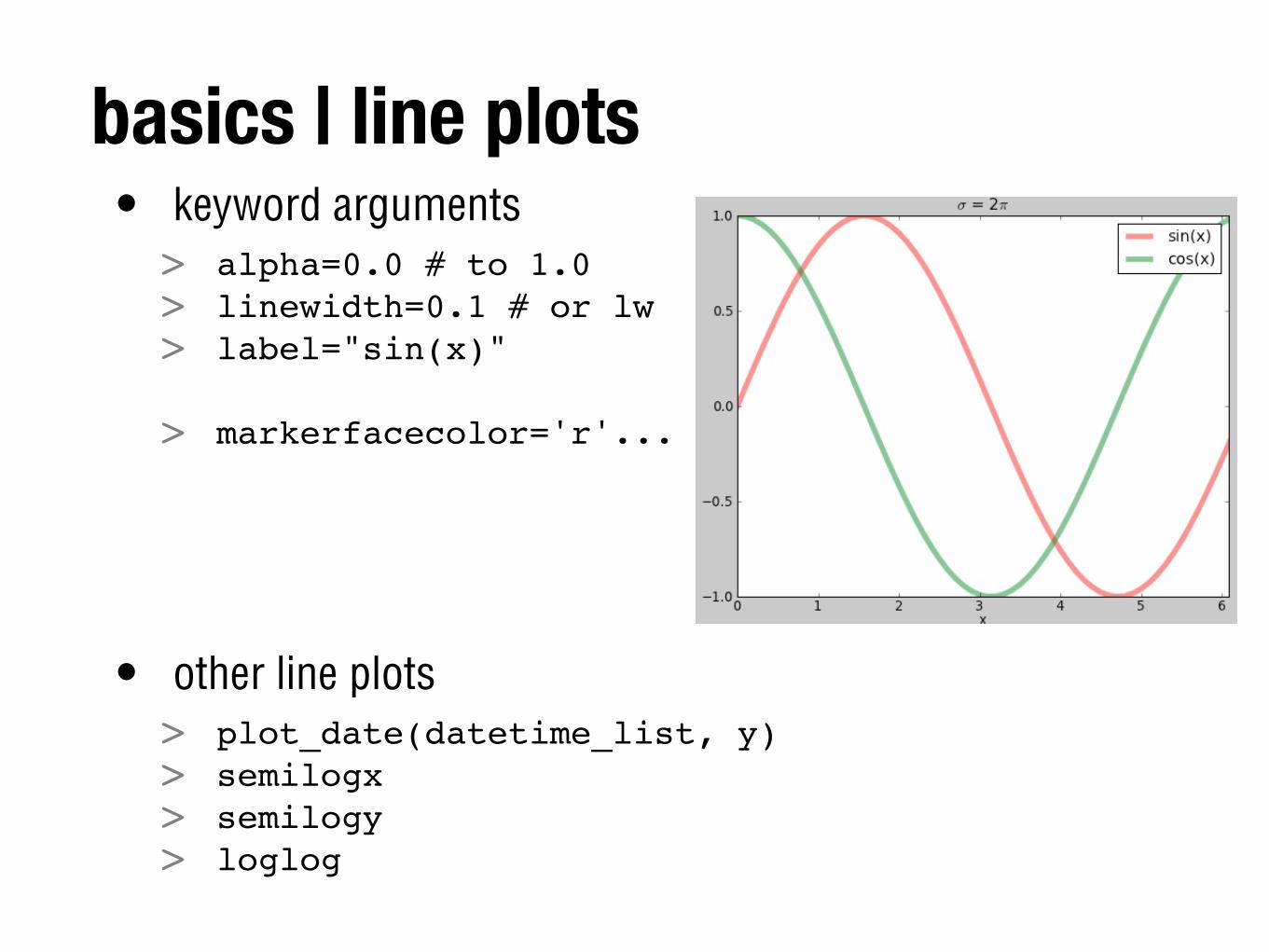
basics | line plots• keyword arguments> alpha=0.0 # to 1.0> linewidth=0.1 # or lw> label="sin(x)"

> markerfacecolor='r'...

• other line plots> plot_date(datetime_list, y)> semilogx> semilogy> loglog

figures

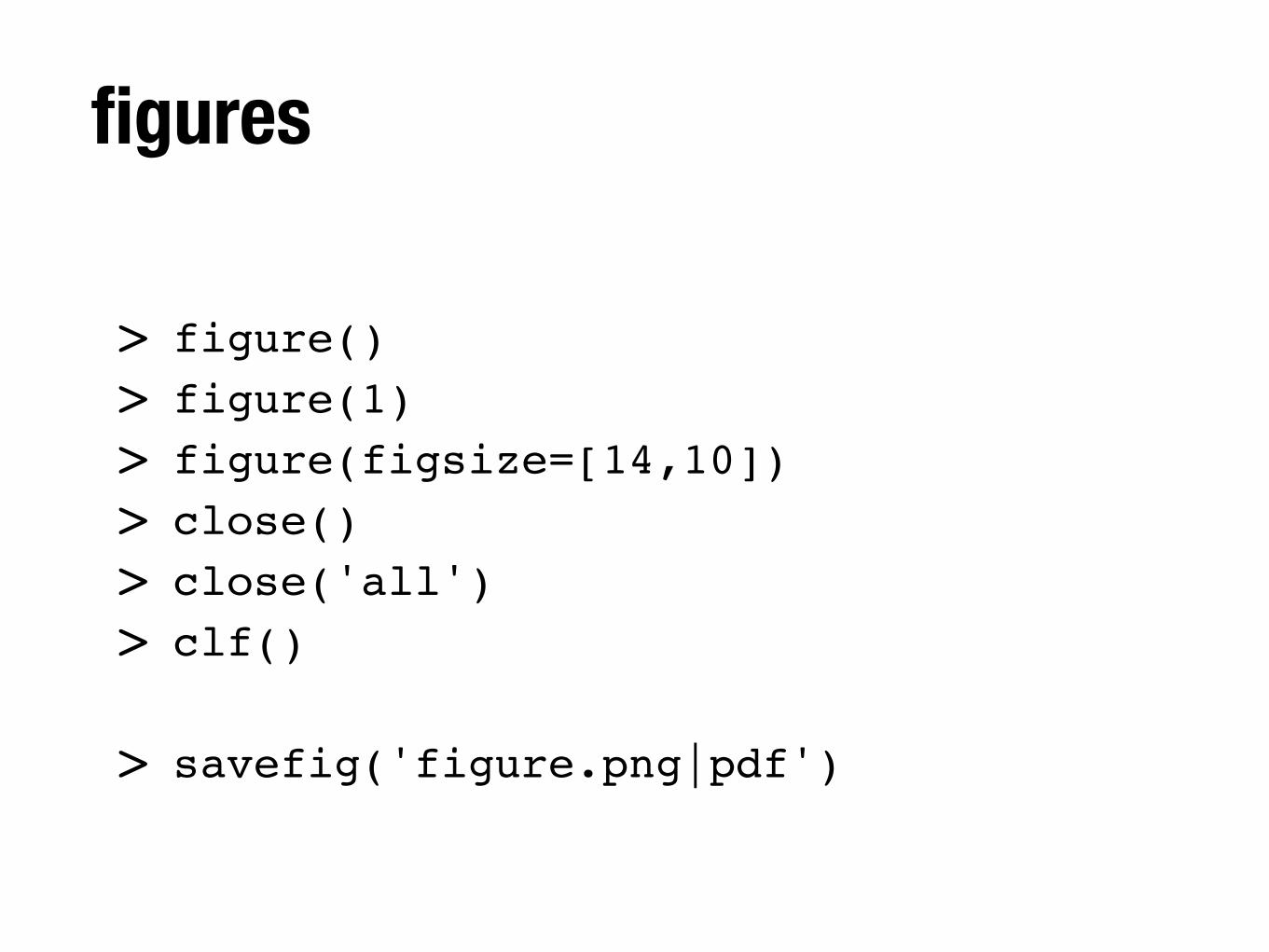
> figure()> figure(1)> figure(figsize=[14,10])> close()> close('all')> clf()

> savefig('figure.png|pdf')

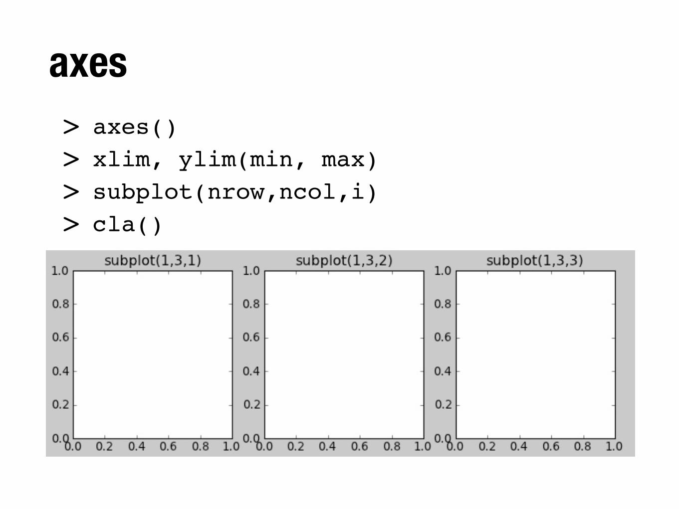
axes> axes()> xlim, ylim(min, max)> subplot(nrow,ncol,i)> cla()

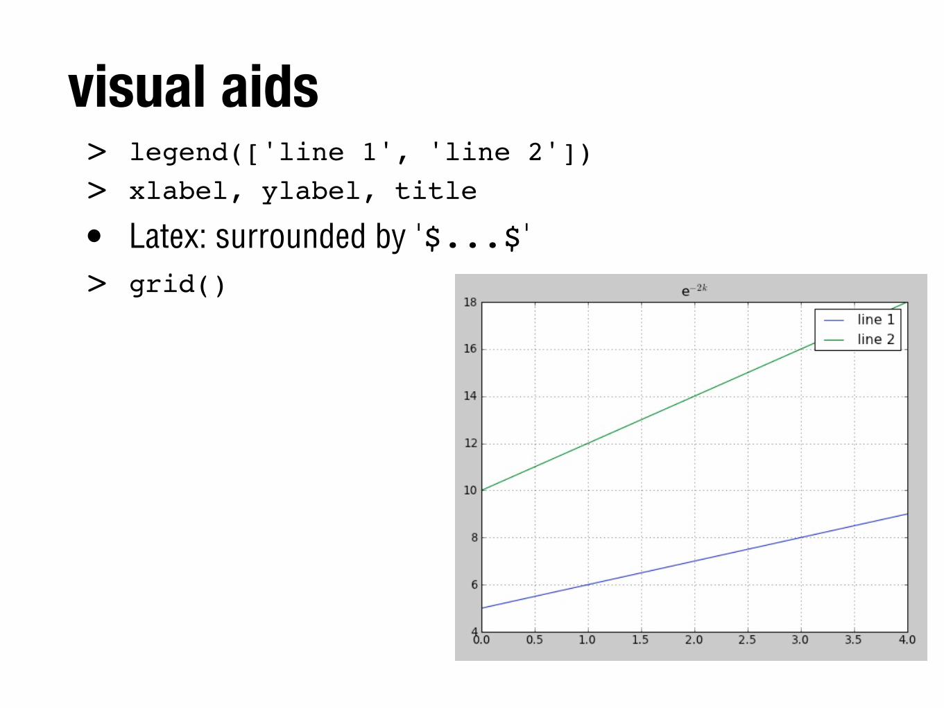
visual aids> legend(['line 1', 'line 2'])> xlabel, ylabel, title

• Latex: surrounded by '$...$'> grid()

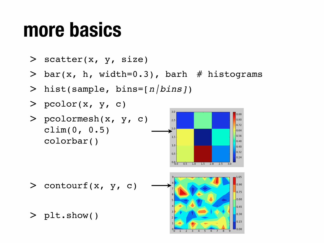
more basics> scatter(x, y, size)

> bar(x, h, width=0.3), barh! # histograms

> hist(sample, bins=[n|bins])

> pcolor(x, y, c)

> pcolormesh(x, y, c)clim(0, 0.5)colorbar()

> contourf(x, y, c)

> plt.show()

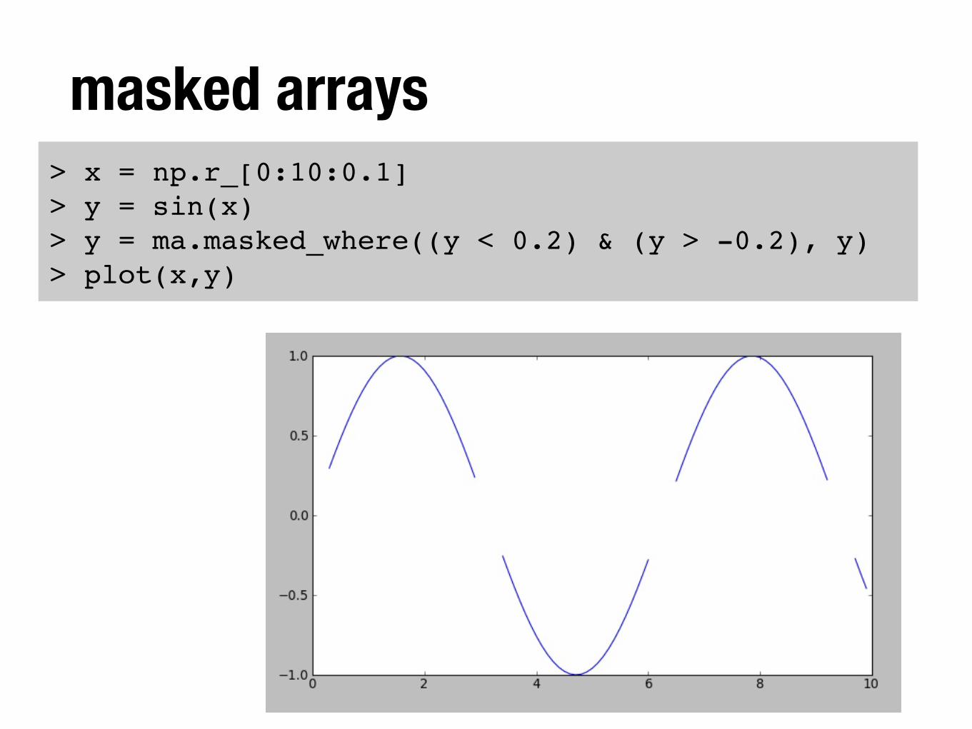
masked arrays> x = np.r_[0:10:0.1]> y = sin(x)> y = ma.masked_where((y < 0.2) & (y > -0.2), y)> plot(x,y)

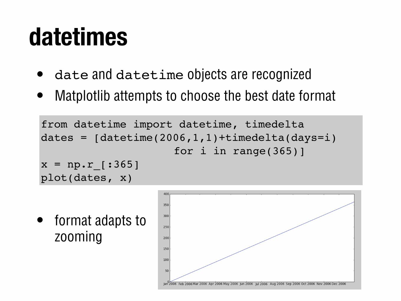
datetimes• date and datetime objects are recognized

• Matplotlib attempts to choose the best date format

• format adapts tozooming

from datetime import datetime, timedeltadates = [datetime(2006,1,1)+timedelta(days=i)! ! ! ! ! ! ! for i in range(365)]x = np.r_[:365]plot(dates, x)

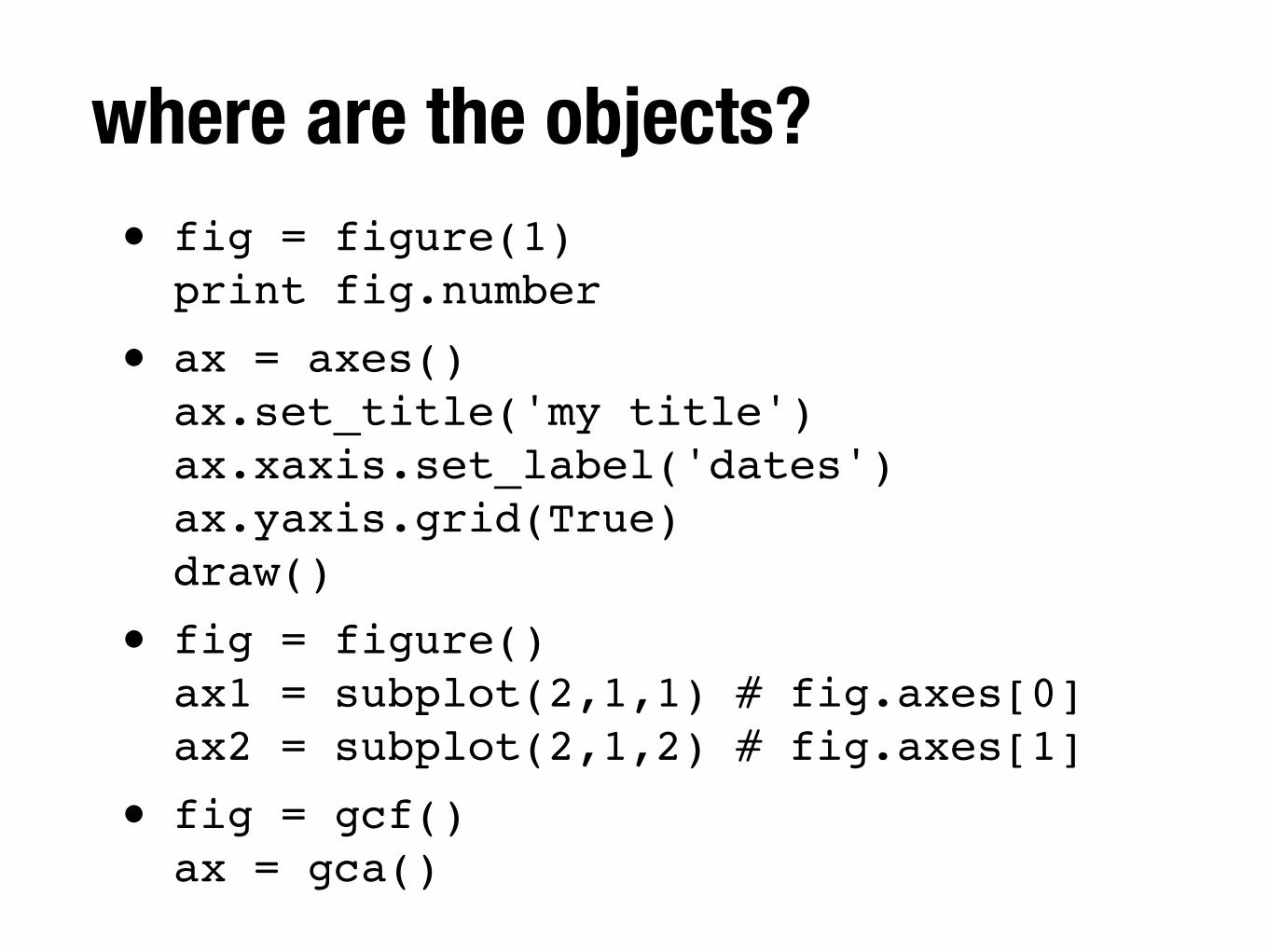
where are the objects?• fig = figure(1)

print fig.number

• ax = axes()ax.set_title('my title')ax.xaxis.set_label('dates')ax.yaxis.grid(True)draw()

• fig = figure()ax1 = subplot(2,1,1) # fig.axes[0]ax2 = subplot(2,1,2) # fig.axes[1]

• fig = gcf()ax = gca()

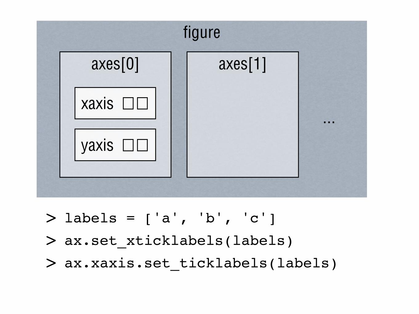
figure

axes[0] axes[1]

xaxis

yaxis

...

> labels = ['a', 'b', 'c']

> ax.set_xticklabels(labels)

> ax.xaxis.set_ticklabels(labels)

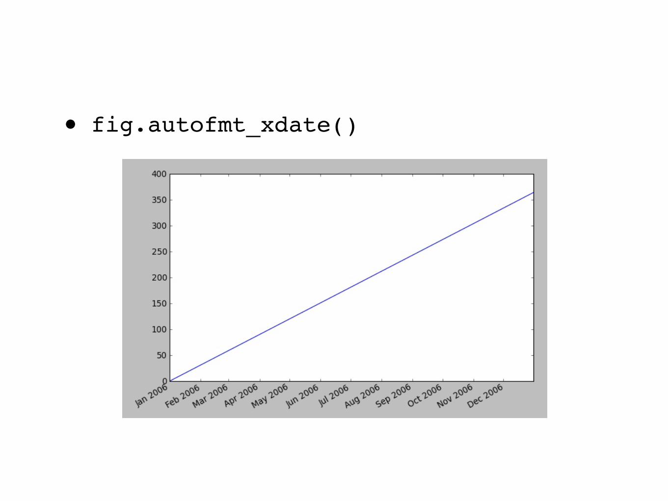
• fig.autofmt_xdate()

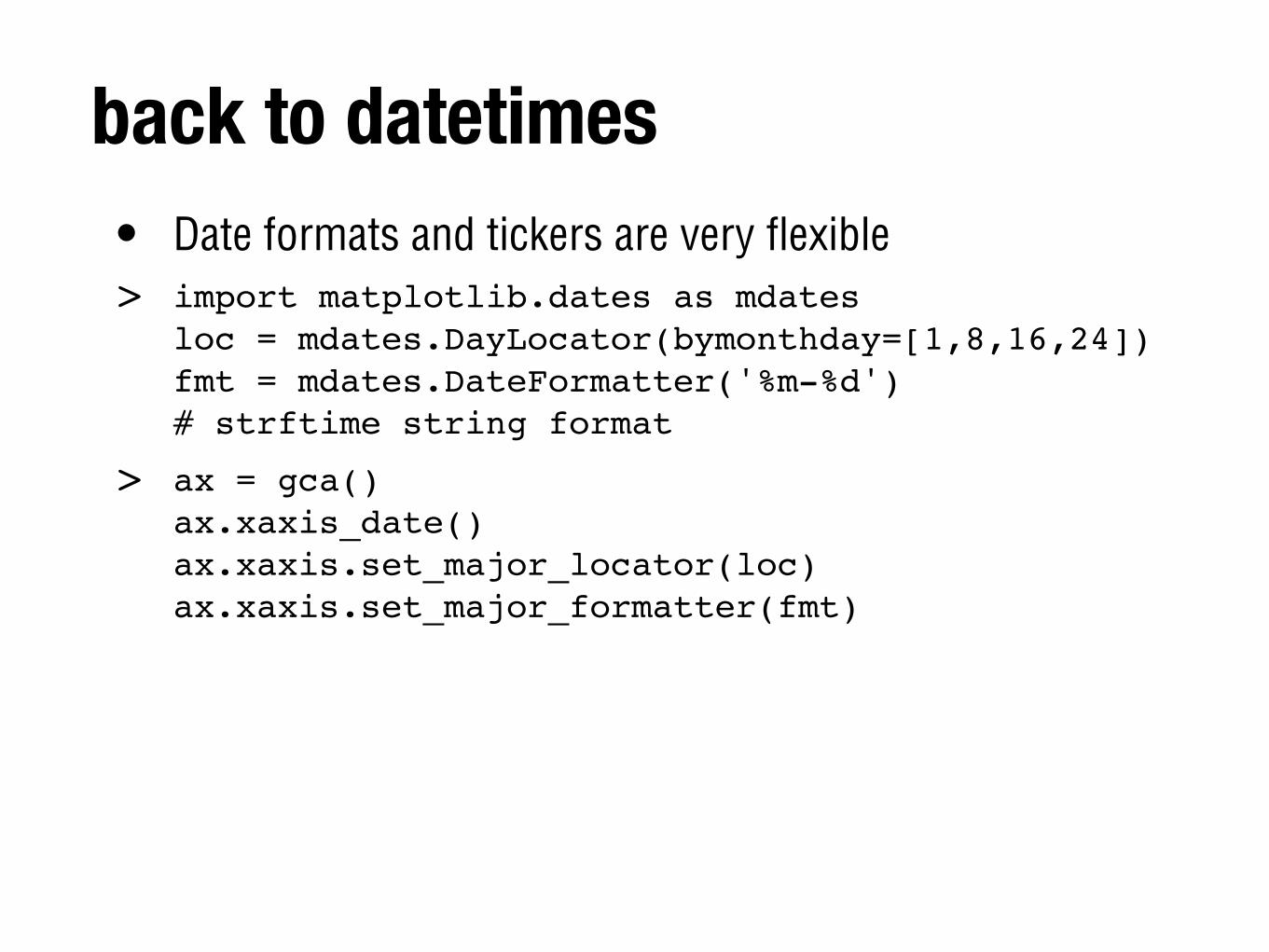
back to datetimes• Date formats and tickers are very flexible> import matplotlib.dates as mdates

loc = mdates.DayLocator(bymonthday=[1,8,16,24])fmt = mdates.DateFormatter('%m-%d')# strftime string format

> ax = gca()ax.xaxis_date()ax.xaxis.set_major_locator(loc)ax.xaxis.set_major_formatter(fmt)

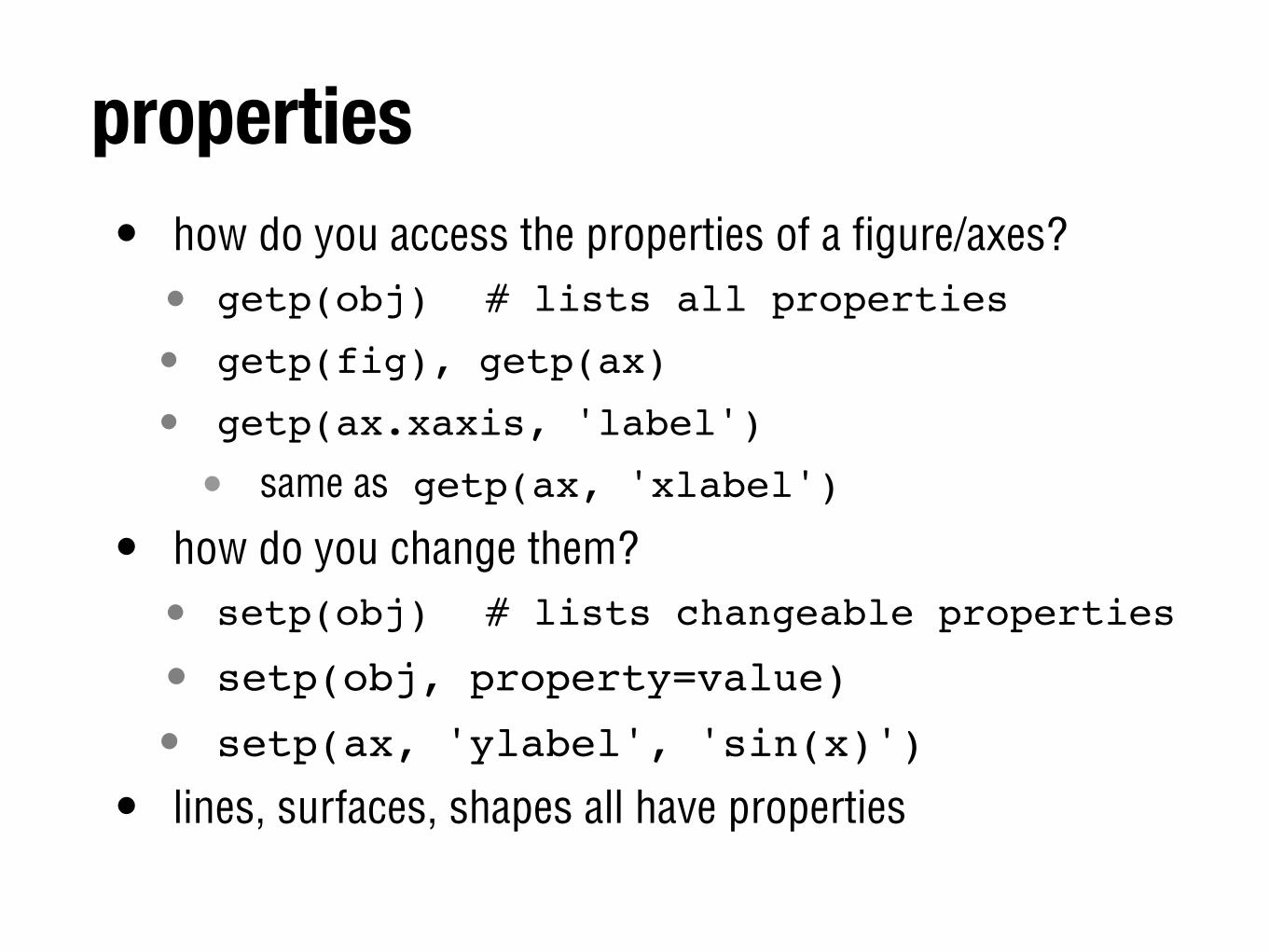
properties• how do you access the properties of a figure/axes?• getp(obj)! # lists all properties

• getp(fig), getp(ax)

• getp(ax.xaxis, 'label')

• same as getp(ax, 'xlabel')

• how do you change them?• setp(obj)! # lists changeable properties

• setp(obj, property=value)

• setp(ax, 'ylabel', 'sin(x)')

• lines, surfaces, shapes all have properties

properties

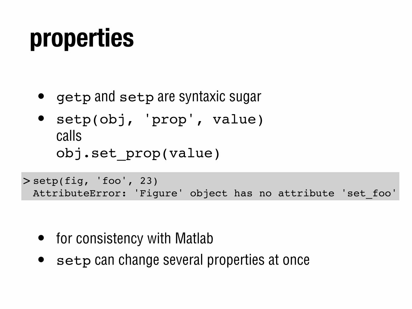
• getp and setp are syntaxic sugar

• setp(obj, 'prop', value) callsobj.set_prop(value)

• for consistency with Matlab

• setp can change several properties at once

> setp(fig, 'foo', 23)AttributeError: 'Figure' object has no attribute 'set_foo'

properties: recap

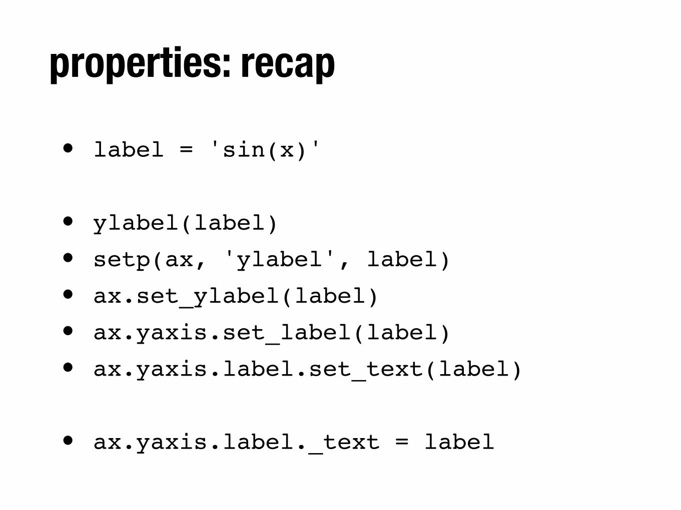
• label = 'sin(x)'

• ylabel(label)

• setp(ax, 'ylabel', label)

• ax.set_ylabel(label)

• ax.yaxis.set_label(label)

• ax.yaxis.label.set_text(label)

• ax.yaxis.label._text = label

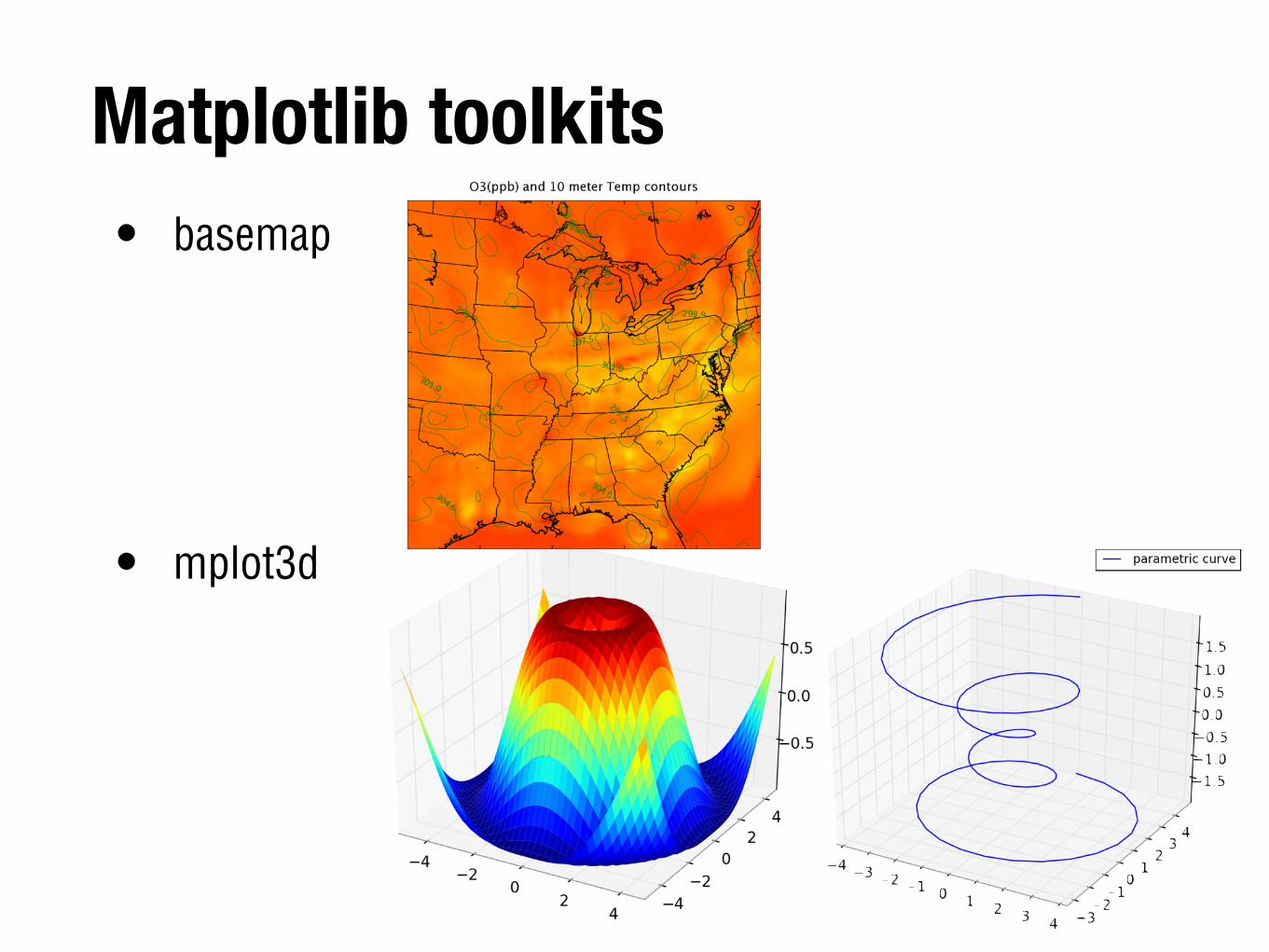
Matplotlib toolkits• basemap

• mplot3d

Matplotlib | documentation• Plotting commands are documented on the matplotlib

homepagehttp://matplotlib.sourceforge.net

• help plotting

• Goot starting point: Matplotlib galleryhttp://matplotlib.sourceforge.net/gallery.html

2. The Python Scientific Stack

4. I/O

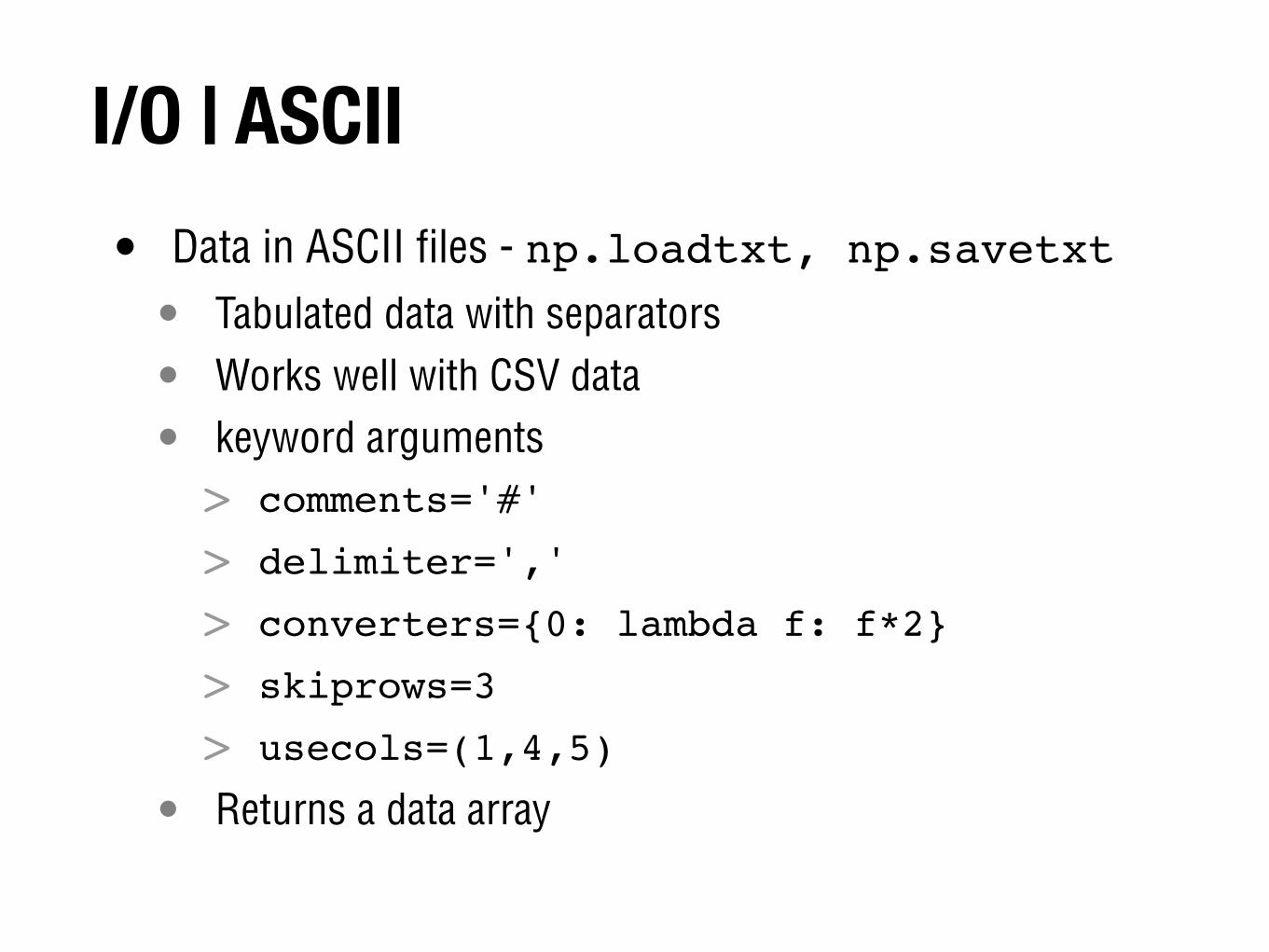
I/O | ASCII• Data in ASCII files - np.loadtxt, np.savetxt

• Tabulated data with separators

• Works well with CSV data

• keyword arguments> comments='#'

> delimiter=','

> converters={0: lambda f: f*2}

> skiprows=3

> usecols=(1,4,5)

• Returns a data array

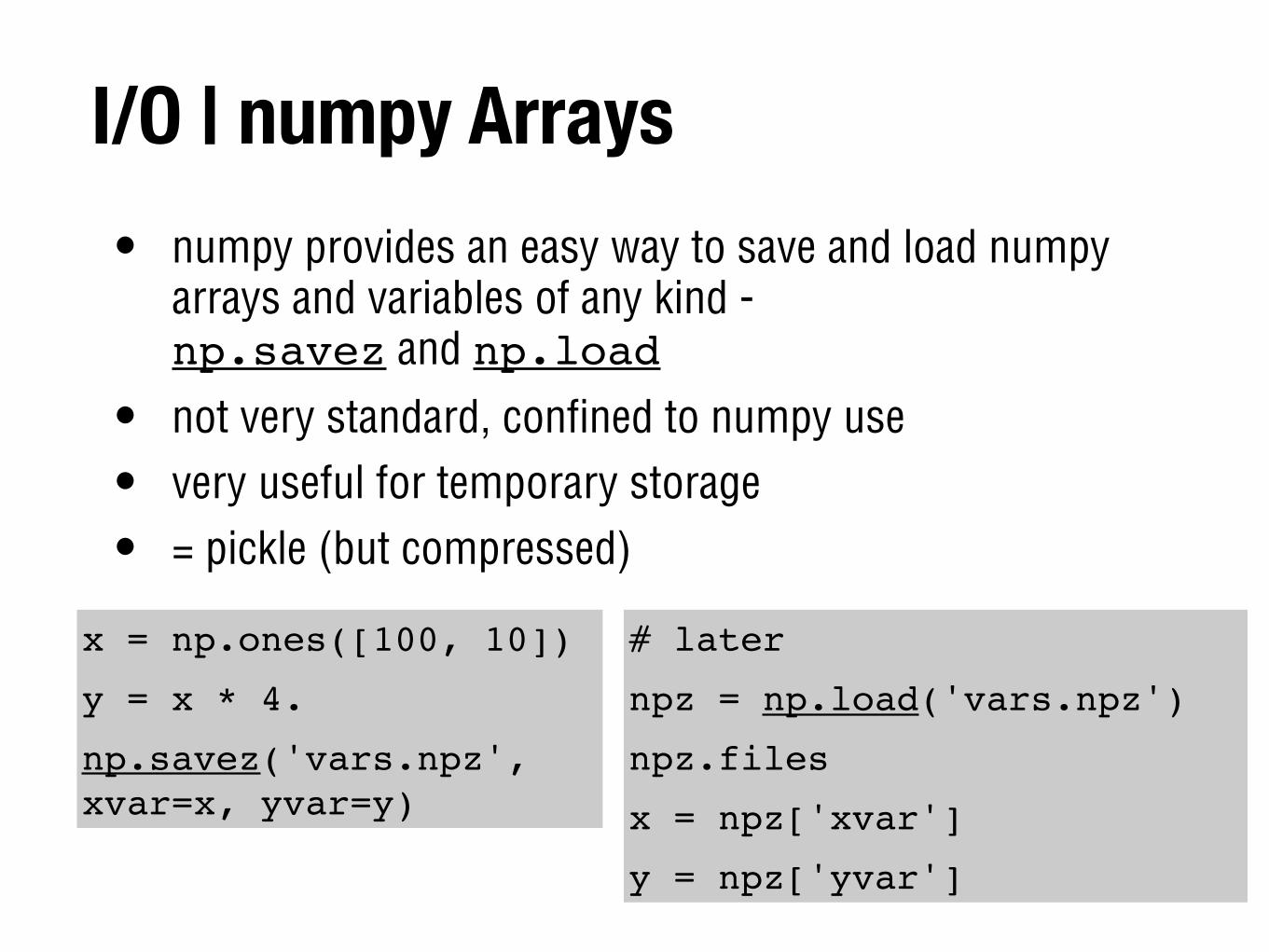
I/O | numpy Arrays• numpy provides an easy way to save and load numpy

arrays and variables of any kind - np.savez and np.load

• not very standard, confined to numpy use

• very useful for temporary storage

• = pickle (but compressed)

x = np.ones([100, 10])

y = x * 4.

np.savez('vars.npz', xvar=x, yvar=y)

# later

npz = np.load('vars.npz')

npz.files

x = npz['xvar']

y = npz['yvar']

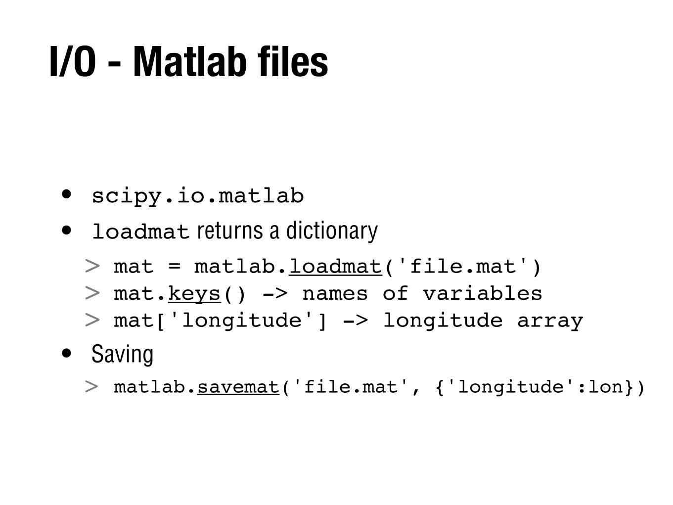
I/O - Matlab files

• scipy.io.matlab

• loadmat returns a dictionary> mat = matlab.loadmat('file.mat')> mat.keys() -> names of variables> mat['longitude'] -> longitude array

• Saving> matlab.savemat('file.mat', {'longitude':lon})

I/O | scientific datasets

• You might need to read and write datasets in structured and autodocumented file formats such as HDF or netCDF

• netcdf4-python

• read and write netCDF3/4 files as Python dictionaries

• supports data compression and packing

• pyhdf, pyh5, pytables : HDF4 and 5 datasets

• pyNIO : GRIB1, GRIB2, HDF-EOS

• in Python(x,y)

• very good online documentation

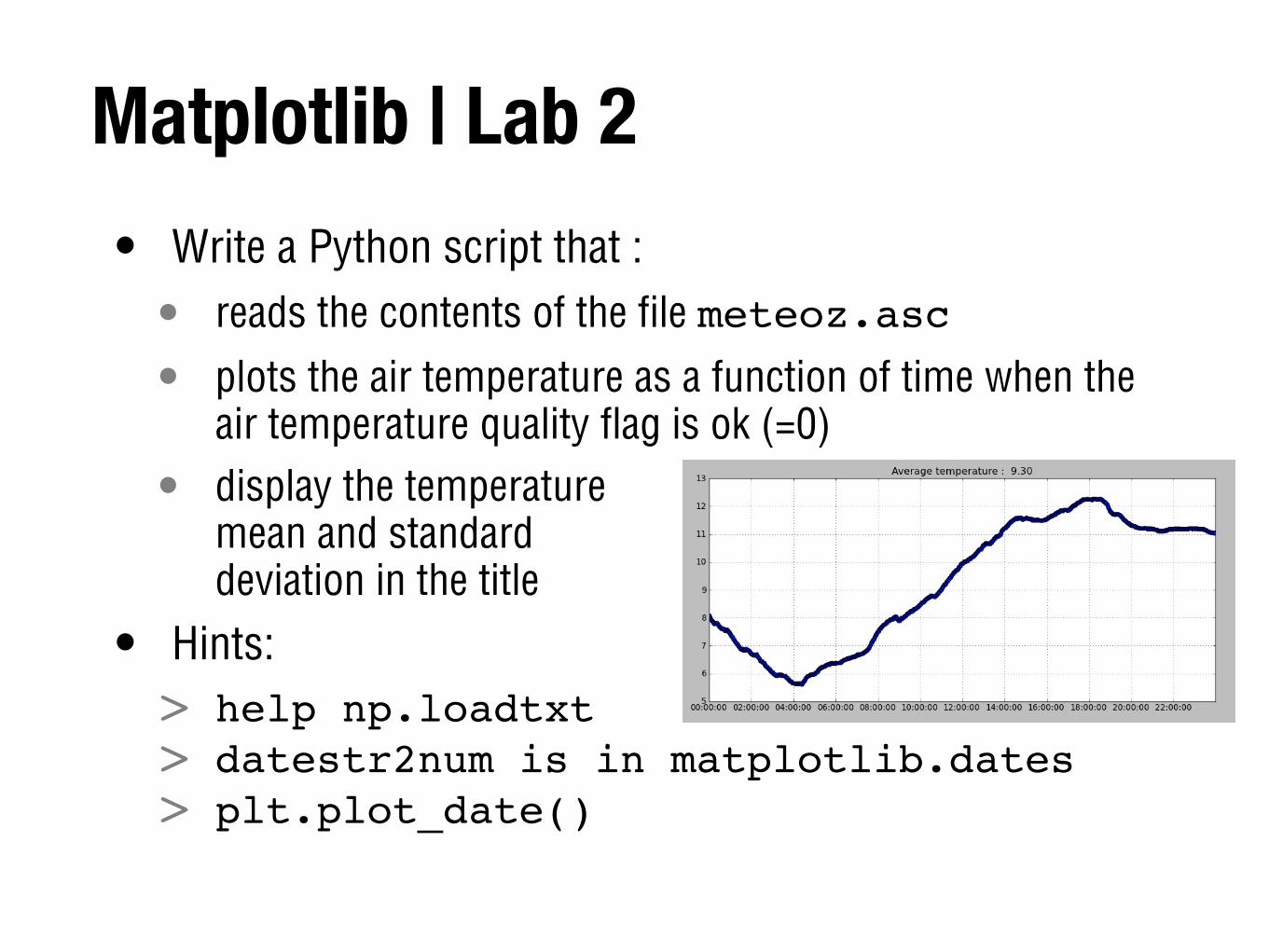
Matplotlib | Lab 2• Write a Python script that :

• reads the contents of the file meteoz.asc

• plots the air temperature as a function of time when the air temperature quality flag is ok (=0)

• display the temperaturemean and standarddeviation in the title

• Hints:> help np.loadtxt> datestr2num is in matplotlib.dates> plt.plot_date()

3. Applications

3. Applications1. Data Analysis

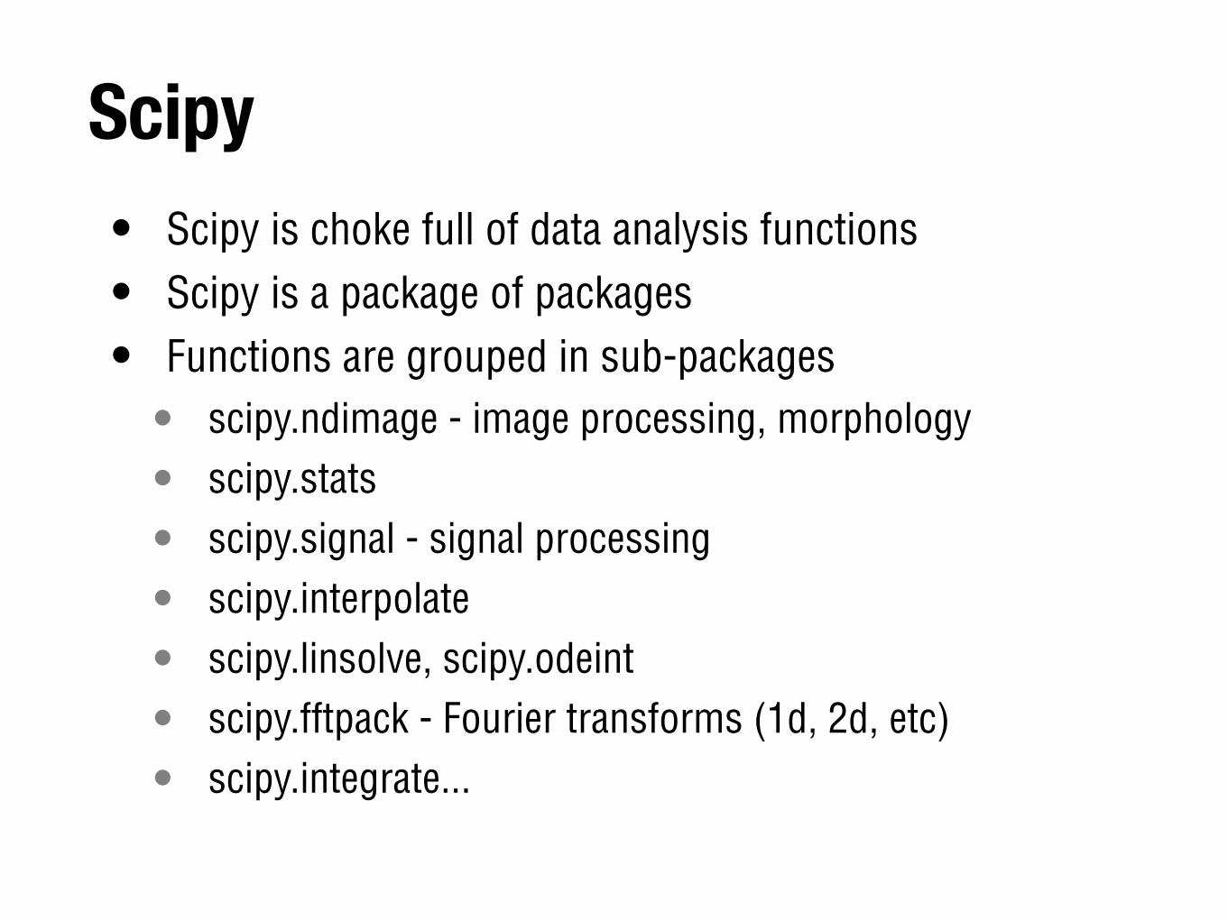
Scipy• Scipy is choke full of data analysis functions

• Scipy is a package of packages

• Functions are grouped in sub-packages• scipy.ndimage - image processing, morphology

• scipy.stats

• scipy.signal - signal processing

• scipy.interpolate

• scipy.linsolve, scipy.odeint

• scipy.fftpack - Fourier transforms (1d, 2d, etc)

• scipy.integrate...

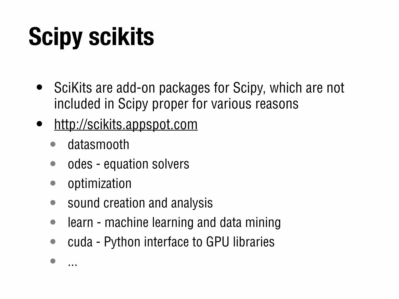
Scipy scikits

• SciKits are add-on packages for Scipy, which are not included in Scipy proper for various reasons

• http://scikits.appspot.com • datasmooth

• odes - equation solvers

• optimization

• sound creation and analysis

• learn - machine learning and data mining

• cuda - Python interface to GPU libraries

• ...

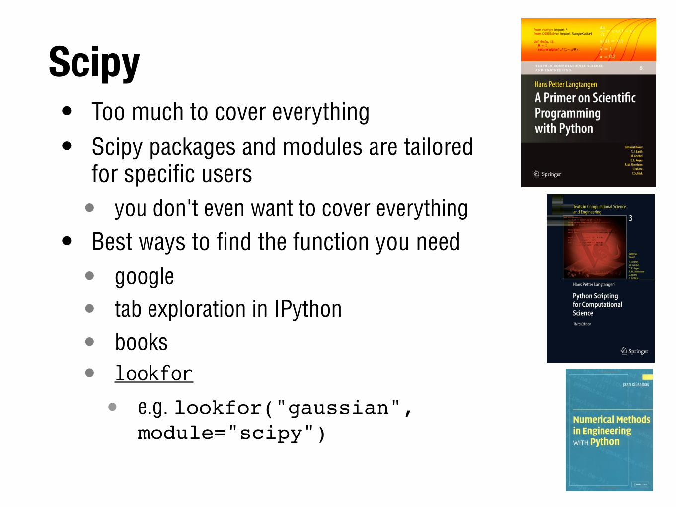
Scipy• Too much to cover everything

• Scipy packages and modules are tailoredfor specific users• you don't even want to cover everything

• Best ways to find the function you need• google

• tab exploration in IPython

• books• lookfor

• e.g. lookfor("gaussian", module="scipy")

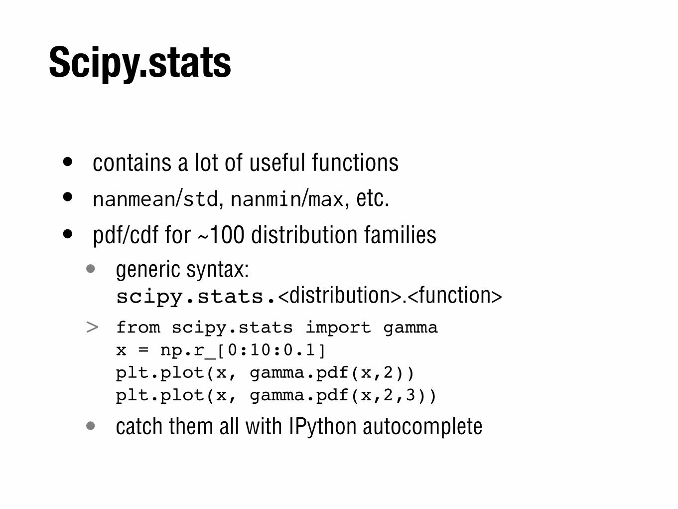
Scipy.stats

• contains a lot of useful functions

• nanmean/std, nanmin/max, etc.

• pdf/cdf for ~100 distribution families• generic syntax:

scipy.stats.<distribution>.<function>> from scipy.stats import gamma

x = np.r_[0:10:0.1]plt.plot(x, gamma.pdf(x,2))plt.plot(x, gamma.pdf(x,2,3))

• catch them all with IPython autocomplete

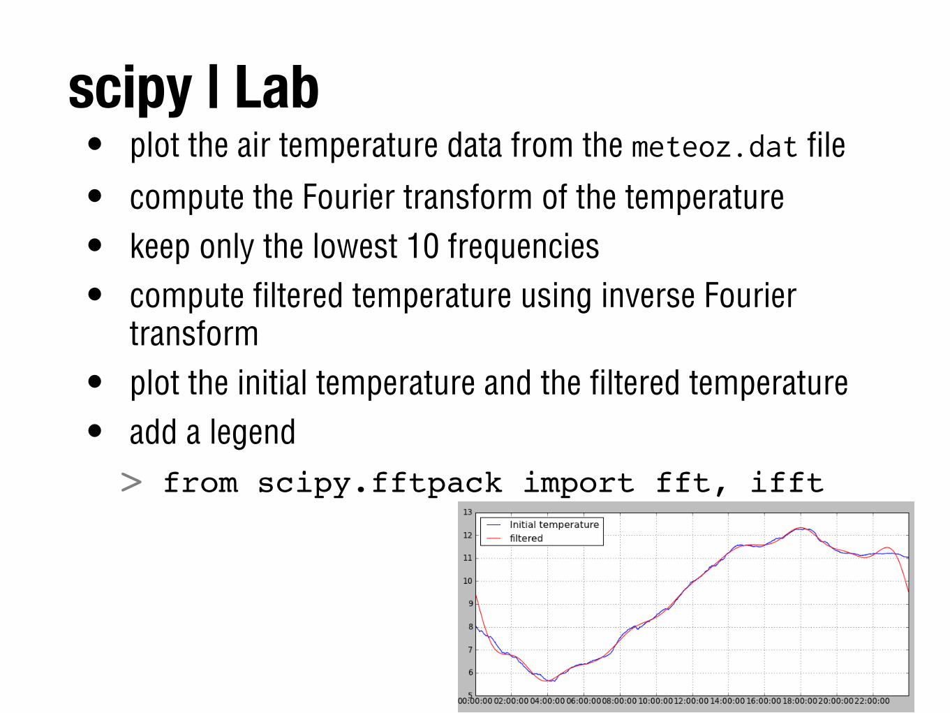
scipy | Lab• plot the air temperature data from the meteoz.dat file

• compute the Fourier transform of the temperature

• keep only the lowest 10 frequencies

• compute filtered temperature using inverse Fourier transform

• plot the initial temperature and the filtered temperature

• add a legend> from scipy.fftpack import fft, ifft

3. Applications

2. Image analysis and filtering

imread

• imread() reads the content of an image file in an array

> img = imread('image.jpg')

• img is [ny, nx, 3]

• [ny, nx] for greyscale images

> imshow(), imsave()

• (0,0) is upper-left

> imshow(img[::-1,:])

• Functions provided by matplotlib.pyplot

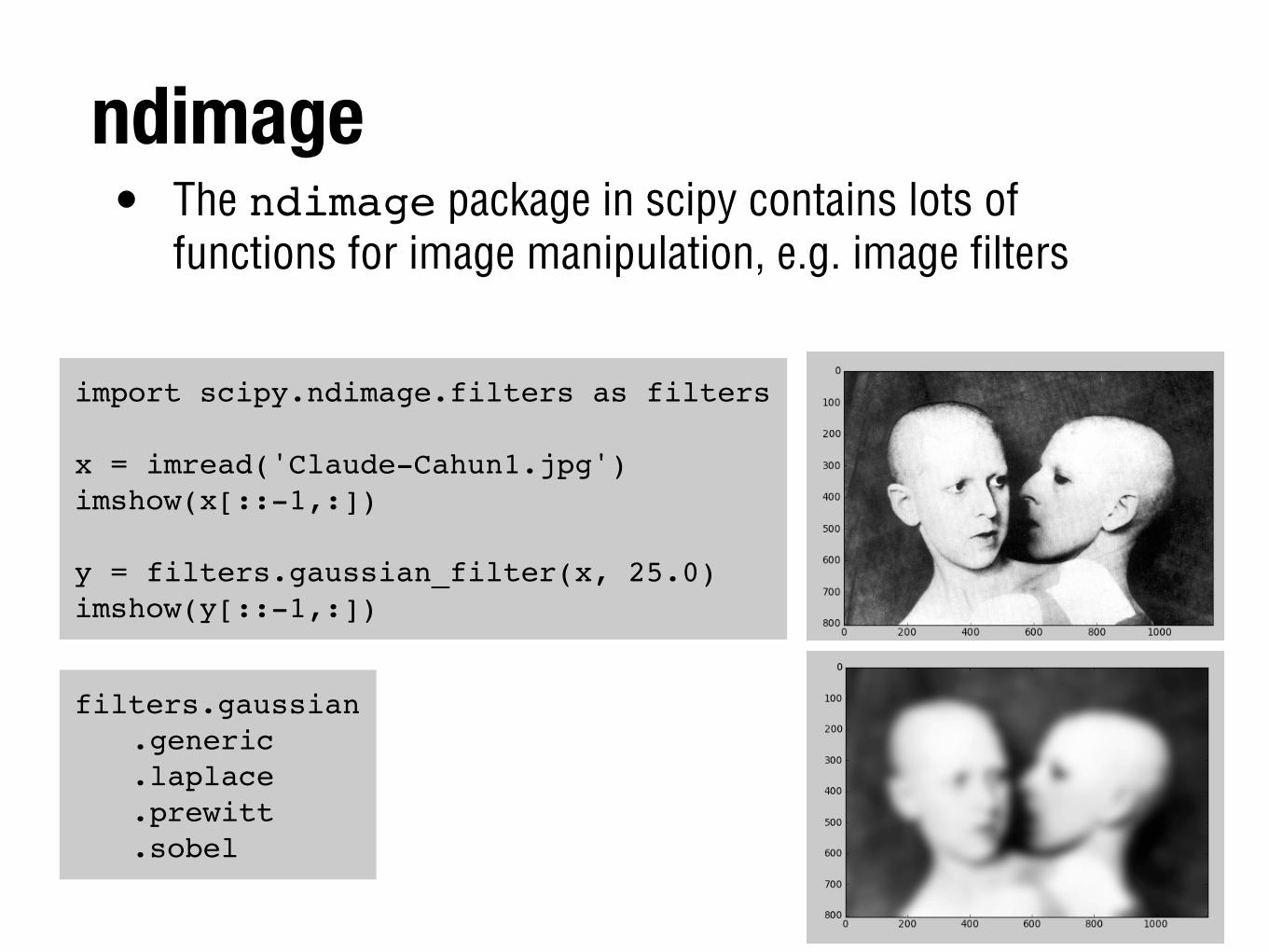
ndimage• The ndimage package in scipy contains lots of

functions for image manipulation, e.g. image filters

import scipy.ndimage.filters as filters

x = imread('Claude-Cahun1.jpg')imshow(x[::-1,:])

y = filters.gaussian_filter(x, 25.0)imshow(y[::-1,:])

filters.gaussian! .generic! .laplace! .prewitt! .sobel

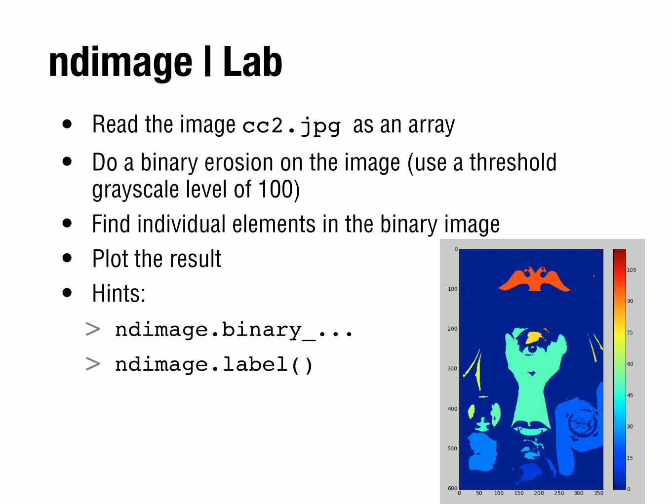
ndimage | Lab• Read the image cc2.jpg as an array

• Do a binary erosion on the image (use a threshold grayscale level of 100)

• Find individual elements in the binary image

• Plot the result

• Hints:> ndimage.binary_...

> ndimage.label()

3. Applications

3. User interaction

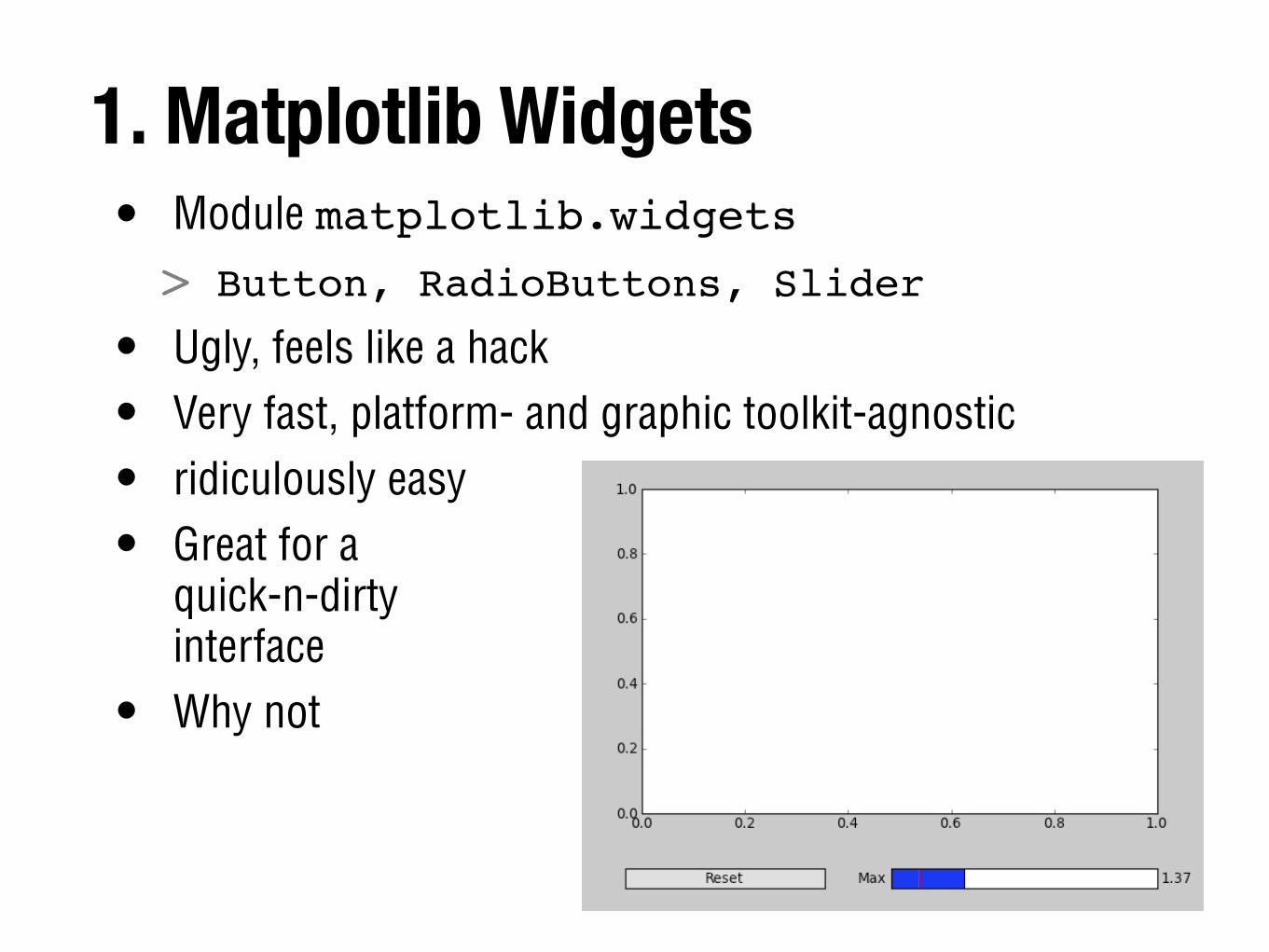
1. Matplotlib Widgets• Module matplotlib.widgets

> Button, RadioButtons, Slider

• Ugly, feels like a hack

• Very fast, platform- and graphic toolkit-agnostic

• ridiculously easy

• Great for aquick-n-dirtyinterface

• Why not

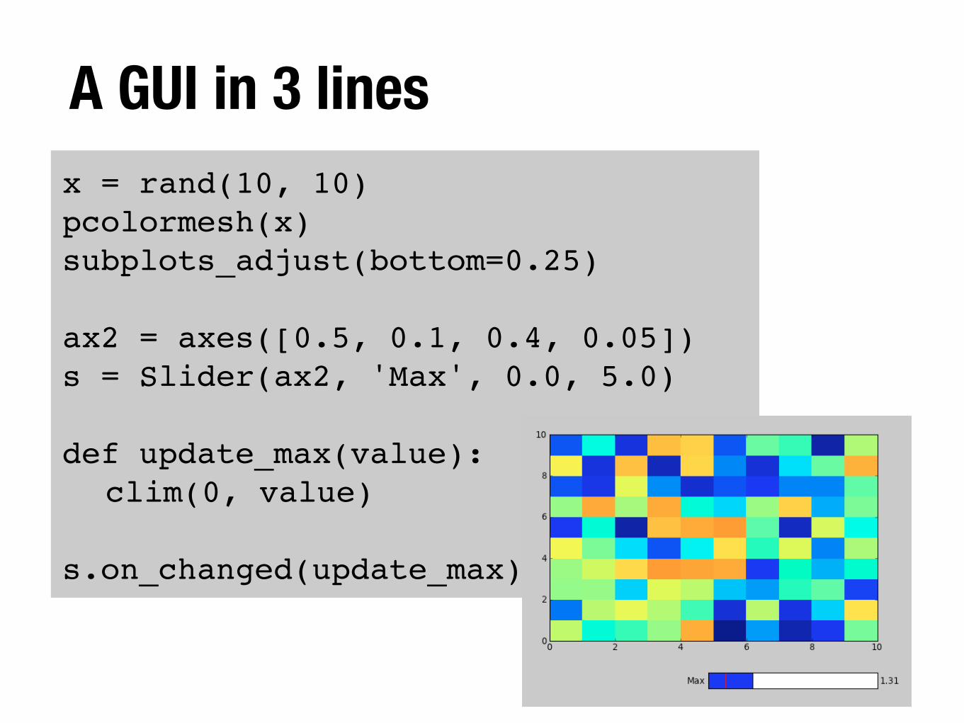
A GUI in 3 linesx = rand(10, 10)pcolormesh(x)subplots_adjust(bottom=0.25)

ax2 = axes([0.5, 0.1, 0.4, 0.05])s = Slider(ax2, 'Max', 0.0, 5.0)

def update_max(value):! clim(0, value)

s.on_changed(update_max)

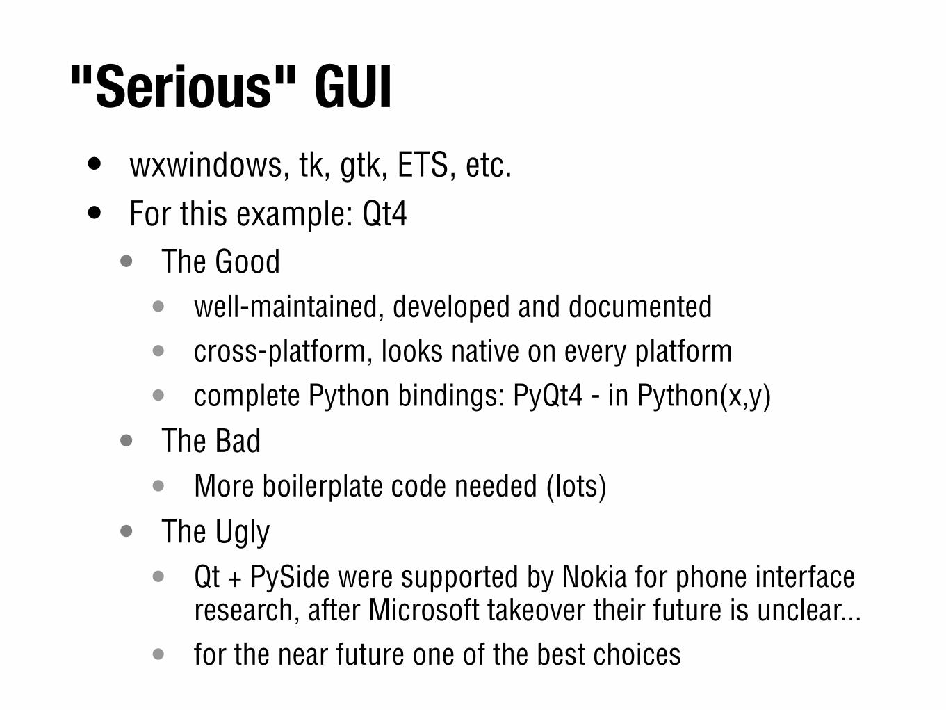
"Serious" GUI• wxwindows, tk, gtk, ETS, etc.

• For this example: Qt4• The Good

• well-maintained, developed and documented

• cross-platform, looks native on every platform

• complete Python bindings: PyQt4 - in Python(x,y)

• The Bad• More boilerplate code needed (lots)

• The Ugly• Qt + PySide were supported by Nokia for phone interface

research, after Microsoft takeover their future is unclear...

• for the near future one of the best choices

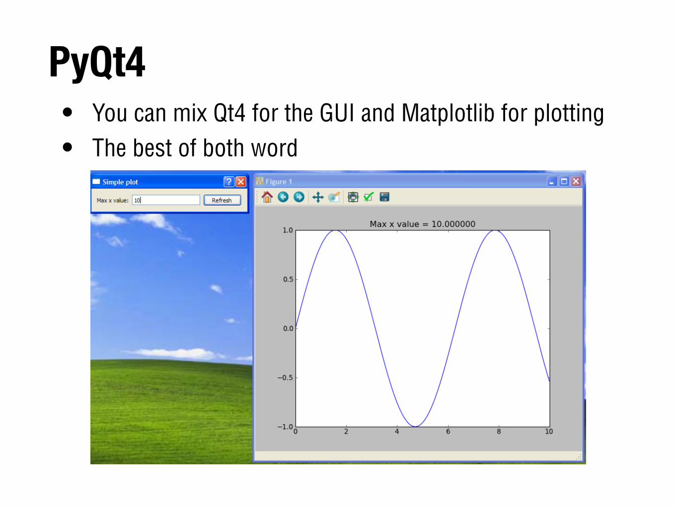
PyQt4• You can mix Qt4 for the GUI and Matplotlib for plotting

• The best of both word

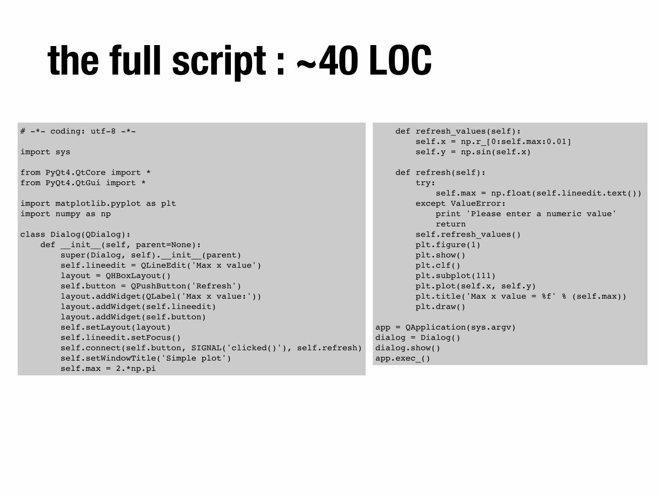
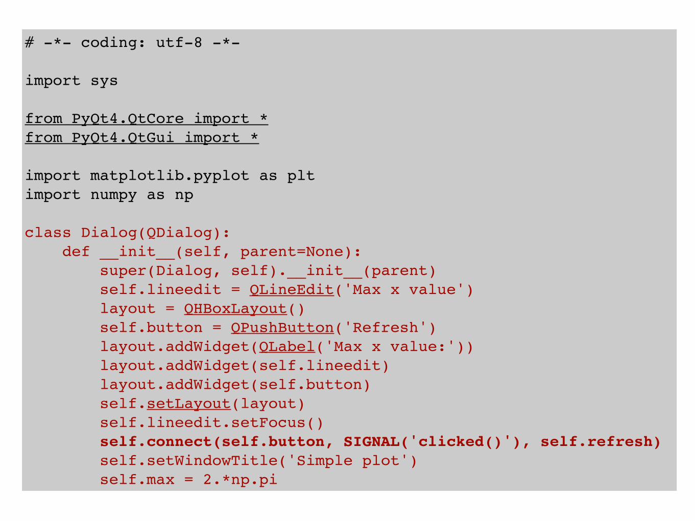
the full script : ~40 LOC# -*- coding: utf-8 -*-

import sys

from PyQt4.QtCore import *from PyQt4.QtGui import *

import matplotlib.pyplot as pltimport numpy as np

class Dialog(QDialog): def __init__(self, parent=None): super(Dialog, self).__init__(parent) self.lineedit = QLineEdit('Max x value') layout = QHBoxLayout() self.button = QPushButton('Refresh') layout.addWidget(QLabel('Max x value:')) layout.addWidget(self.lineedit) layout.addWidget(self.button) self.setLayout(layout) self.lineedit.setFocus() self.connect(self.button, SIGNAL('clicked()'), self.refresh) self.setWindowTitle('Simple plot') self.max = 2.*np.pi

def refresh_values(self): self.x = np.r_[0:self.max:0.01] self.y = np.sin(self.x) def refresh(self): try: self.max = np.float(self.lineedit.text()) except ValueError: print 'Please enter a numeric value' return self.refresh_values() plt.figure(1) plt.show() plt.clf() plt.subplot(111) plt.plot(self.x, self.y) plt.title('Max x value = %f' % (self.max)) plt.draw() app = QApplication(sys.argv)dialog = Dialog()dialog.show()app.exec_()

# -*- coding: utf-8 -*-

import sys

from PyQt4.QtCore import *from PyQt4.QtGui import *

import matplotlib.pyplot as pltimport numpy as np

class Dialog(QDialog): def __init__(self, parent=None): super(Dialog, self).__init__(parent) self.lineedit = QLineEdit('Max x value') layout = QHBoxLayout() self.button = QPushButton('Refresh') layout.addWidget(QLabel('Max x value:')) layout.addWidget(self.lineedit) layout.addWidget(self.button) self.setLayout(layout) self.lineedit.setFocus() self.connect(self.button, SIGNAL('clicked()'), self.refresh) self.setWindowTitle('Simple plot') self.max = 2.*np.pi

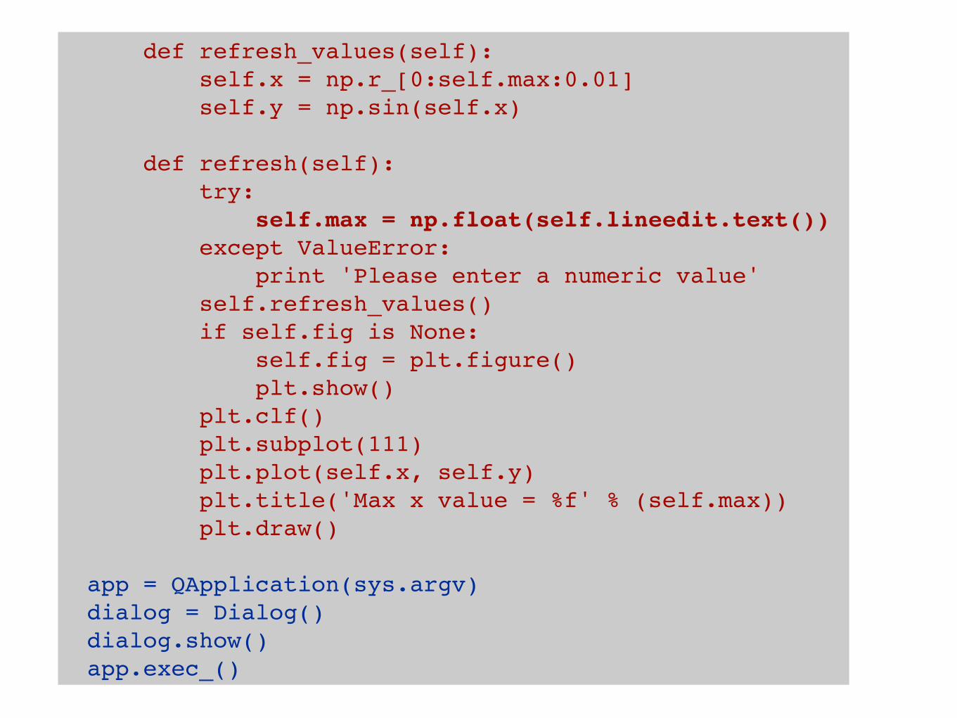
def refresh_values(self): self.x = np.r_[0:self.max:0.01] self.y = np.sin(self.x) def refresh(self): try: self.max = np.float(self.lineedit.text()) except ValueError: print 'Please enter a numeric value' self.refresh_values() if self.fig is None: self.fig = plt.figure() plt.show() plt.clf() plt.subplot(111) plt.plot(self.x, self.y) plt.title('Max x value = %f' % (self.max)) plt.draw() app = QApplication(sys.argv)dialog = Dialog()dialog.show()app.exec_()

GUI | Lab• Modify this script so the interface shows two buttons

• one for plotting cos(x)

• one for plotting sin(x)

thanks