DIVERSITY AND DEVELOPMENT IN CALIFORNIA CITIES€¦ · 100% sample of responses to the short form questions on the 1990 census, while the language variable is based on a roughly 1-in-7

DIVERSITY AND DEVELOPMENT IN CALIFORNIA CITIES

A Quantitative Study of Local Economic Growth

A Planning Report Presented to

The Faculty of the Department of Urban and Regional Planning

San Jose State University

In Partial Fulfillment

Of the Requirements for the Degree Master of Urban Planning

By Matt Piven

December 2010

Diversity and Development in California Cities • December 13, 2010 Page ii

TABLE OF CONTENTS

LIST OF FIGURES ......................................................................................................... V

LIST OF TABLES.......................................................................................................... VI

ACKNOWLEDGMENTS............................................................................................... VII

I. INTRODUCTION....................................................................................................... 1

A. Background .................................................................................................................................................................1 1. Why Study California’s Urban Economic Growth?...............................................................................................1 2. How to Study Population Diversity.........................................................................................................................2 3. Why Study Population Diversity? ...........................................................................................................................4 4. Overview of Methods ...............................................................................................................................................5

B. Research Question ......................................................................................................................................................8

C. Relevance .....................................................................................................................................................................8 1. Contribution to Urban Economic Growth Literature .............................................................................................8 2. Applications to Planning Practice............................................................................................................................9

D. Report Structure...................................................................................................................................................... 12

II. LITERATURE REVIEW ......................................................................................... 13

A. Introduction.............................................................................................................................................................. 13

B. Relationship between Population Diversity and Economic Activity ............................................................... 13 1. Empirical Studies ................................................................................................................................................... 13 2. Theoretical Concepts from the Literature ............................................................................................................ 17 3. Conclusions ............................................................................................................................................................ 21

C. Previous Models Which Inform This Project ..................................................................................................... 21 1. Ottaviano and Peri ................................................................................................................................................. 22 2. Glaeser et al............................................................................................................................................................ 23 3. Stansel..................................................................................................................................................................... 25 4. Cheshire and Carbonaro ........................................................................................................................................ 26

III. MODEL STATEMENT .......................................................................................... 27

A. Problem Description ............................................................................................................................................... 27

Diversity and Development in California Cities • December 13, 2010 Page iii

B. Primary Assumptions ............................................................................................................................................. 27

C. Primary Derivations................................................................................................................................................ 28

D. Secondary Assumptions.......................................................................................................................................... 29

E. Secondary Derivations ............................................................................................................................................ 30

IV. EMPIRICAL ANALYSIS ....................................................................................... 33

A. Introduction.............................................................................................................................................................. 33

B. Data............................................................................................................................................................................ 33 1. Empirical Strategy ................................................................................................................................................. 33 2. Sources ................................................................................................................................................................... 35 3. Descriptive Statistics ............................................................................................................................................. 35

C. Methods..................................................................................................................................................................... 42 1. Base Model............................................................................................................................................................. 42 2. Diversity Model ..................................................................................................................................................... 44 3. Benefits of City-Level Analysis Over Smaller Scales ........................................................................................ 44

D. Hypotheses................................................................................................................................................................ 44

E. Results ....................................................................................................................................................................... 45 1. Comparing Base Model 1 to Glaeser et al. .......................................................................................................... 45 2. Comparing Base Model 2 to Stansel .................................................................................................................... 46 3. Diversity Model Results ........................................................................................................................................ 46

F. Limitations ................................................................................................................................................................ 49 1. Changing City Boundaries .................................................................................................................................... 49 2. Changing Sets of Cities ......................................................................................................................................... 50 3. Changing MSA Definitions .................................................................................................................................. 50

V. CONCLUSIONS .................................................................................................... 51

A. Lessons Learned from Empirical Analysis ......................................................................................................... 51

B. Contributions to Existing Literature.................................................................................................................... 51

C. Future Directions and Implications for Planners............................................................................................... 52

VI. BIBLIOGRAPHY .................................................................................................. 55

Diversity and Development in California Cities • December 13, 2010 Page iv

APPENDICES............................................................................................................... 59 1. Map Production...................................................................................................................................................... 59 2. Why Certain Cities Were Excluded...................................................................................................................... 60 3. Census Variable Codes Used ................................................................................................................................ 60 4. Why the Area-Related Control Was Excluded .................................................................................................... 60 5. MSA-Level Values of the Diversity Variables .................................................................................................... 61

Diversity and Development in California Cities • December 13, 2010 Page v

LIST OF FIGURES Figure I-1. Ethnic Diversity in California’s Cities, 1990....................................................................................................6 Figure I-2. Linguistic Diversity in California’s Cities, 1990..............................................................................................7 Figure IV-1. Frequency Distribution for Ethnic Diversity Variables. ............................................................................ 40 Figure IV-2. Comparison of 1990 Ethnic Diversity Data Across Aggregation Levels. ................................................ 41 Figure IV-3. Frequency Histogram of Percent Changes in City Areas, 1990-2000. ..................................................... 49

Diversity and Development in California Cities • December 13, 2010 Page vi

LIST OF TABLES Table I-1. Ethnic and Linguistic Groups Defined by 1990 U.S. Census. ..........................................................................3 Table IV-1. Connection Between Model Elements and Empirical Variables. ............................................................... 33 Table IV-2. Names and Definitions for all Variables Used in Analysis......................................................................... 36 Table IV-4. Descriptive Statistics for Variables Used in Analysis. ................................................................................ 38 Table IV-5. Regression Results from Stansel and Glaeser et al...................................................................................... 43 Table IV-6. Base Model and Diversity Model Results. ................................................................................................... 47 Table IV-7. Description of Three Groups Separated by MSA Ethnic Diversity Value. ............................................... 48

Diversity and Development in California Cities • December 13, 2010 Page vii

ACKNOWLEDGMENTS

I am indebted to my advisor, Mike Pogodzinksi, a Professor in the San Jose State University Department of Economics. He provided many thoughtful comments which guided the development of this research, and was a constant source of encouragement during the process.

I also benefited from the assistance of Roxanne Ezzet-Lofstrom and Rick Kos, both Lecturers in the San Jose State University Department of Urban and Regional Planning. Roxanne provided many useful comments, and Rick provided feedback on several mapping issues and geoprocessing tasks.

Diversity and Development in California Cities • December 13, 2010 Page viii

I. INTRODUCTION

A. Background

California's economy is the largest of any state in the US, and if it were an independent country, it would rank among the top ten economies in the world in terms of gross domestic product (GDP).1 Yet, in the not-so-distant past, the economy was small, a far cry from the booming technology and entertainment centers that are the envy of the world. Such rapid growth provides an excellent setting in which to test the determinants of economic growth. This report examines the effect of population diversity on economic growth across California’s cities. Understanding the determinants of urban economic growth is crucial to urban planners, and, as discussed later in this chapter, there are numerous ways in which the factors significant to economic growth affect planning practice.

1. Why Study California’s Urban Economic Growth?

There are two reasons to focus on California. First, the outlines of California’s recent economic history are broadly familiar.2 Second, 20th century growth in the state was phenomenally rapid. Between 1963 and 1997, the state’s GDP grew in real terms by a factor of fifteen.3 Growth was also high compared to other states. California had the greatest growth in total personal income of the lower 48 states between 1930 and 2000. In terms of per capita income growth, moreover, California ranked ninth.4

There are several considerations that affect the size and nature of the dataset used in this report.5 We are interested in looking at the role of municipal finance variables, and therefore we use cities as the unit of analysis. The sample of cities used in this report held 74% of the state’s 1990 population.6 Thus, by focusing on municipal areas, we are better able

1 Central Intelligence Agency, “CIA World Factbook,” https://www.cia.gov/library/publications/the-world-factbook/rankorder/2001rank.html (accessed November 17, 2009). 2 California Department of Finance, “A Brief History of the California Economy,” http://www.dof.ca.gov/html/fs_data/HistoryCAEconomy/index.htm (accessed October 15, 2010). 3 U.S. Bureau of Economic Analysis, “Regional Economic Accounts,” http://www.bea.gov/regional/gsp/ (accessed April 11, 2010). 4 U.S. Bureau of Economic Analysis, “State Annual Personal Income,” http://www.bea.gov/regional/spi/ (accessed September 25, 2010). Note that Alaska and Hawaii were not included in this analysis because they were not states in 1930, but the District of Columbia was included. 5 A more complete description of the steps taken to obtain the sample are described in the Data section of the Empirical Analysis chapter. 6 This is based on the sum of the population of the cities, as defined by the 1992 Census of Governments, divided by the Census Bureau’s 1992 estimate of California’s population, found at U.S. Census Bureau, “State Population Estimates,” http://www.census.gov/popest/archives/1990s/ST-99-03.txt (accessed November 7, 2010).

INTRODUCTION

Diversity and Development in California Cities • December 13, 2010 Page 2

to control for the effect of local expenditures, revenues, and debt, which leads to a better model of growth.7

2. How to Study Population Diversity

In this report, the term population diversity8 encompasses two concepts: ethnic diversity and linguistic diversity.

a) Operationalizing the Concept

In this report, the two concepts of ethnic diversity and linguistic diversity are measured in the same way, using different data. Ethnic diversity is measured using the ethnic categories of the 1990 census. Linguistic diversity is measured by using responses to the language spoken at home question in the 1990 census.9 The specific categories of each variable are shown in Table I-1.

Levels of diversity are measured by computing Simpson's Diversity Index (SDI), which is widely used in social and natural sciences to measure diversity.10 The SDI is calculated as follows:

!

SDI =1"ngN

#

$ %

&

' (

2

,g=1

G

)

where the SDI is the value of the index, ng is the number of people in the gth ethnic or linguistic group, N is the population of the area being studied, and G is the number of groups. This index of diversity varies between zero and one, and it represents the likelihood that any two

7 Using cities as a unit of analysis of course reduces the number of observations compared with lower geographic scales. 8 The term ethnolinguistic diversity is also used in the literature. It is interchangeable with population diversity. See Uslaner, Eric. “Does Diversity Drive Down Trust?” Working Paper 69.2006, Fondazione Eni Enrico Mattei, April 2006. 9 The specific census variables are Summary File 1 variable P007 (Detailed Race) and Summary File 3 variable P0031 (Language Spoken at Home). Note that the ethnicity variable is based on a theoretical 100% sample of responses to the short form questions on the 1990 census, while the language variable is based on a roughly 1-in-7 (17%) sample of responses to the long form questions on the 1990 census. 10 For an example of a related paper which uses the index, see Gianmarco I.P. Ottaviano and Giovanni Peri, “Cities and Cultures.” For a discussion of various diversity indices, see Carole Maignan, Gianmarco Ottaviano, Dino Pinelli, and Francesco Rullani, “Bio-Ecological Diversity vs. Socio-Economic Diversity: A Comparison of Existing Measures,” Working Paper #13.2003, Fondazione Eni Enrico Mattei, 2003.

INTRODUCTION


people picked from a population will be of different groups.11 The SDI captures the richness and, especially, the degree of evenness in a population’s composition.

Table I-1. Ethnic and Linguistic Groups Defined by 1990 U.S. Census.

Ethnic Groups Linguistic Groups White Speak only English Black German American Indian Yiddish Eskimo Other West Germanic language Aleut Scandinavian Chinese Greek Filipino Indic Japanese Italian Asian Indian French or French Creole Korean Portuguese or Portuguese Creole Vietnamese Spanish or Spanish Creole Cambodian Polish Hmong Russian Laotian South Slavic Thai Other Slavic language Other Asian Other Indo-European language Hawaiian Arabic Samoan Tagalog Tongan Chinese Other Polynesian Hungarian Guamanian Japanese Other Micronesian Mon-Khmer Melanesian Korean Pacific Islander; not specified Native North American languages Other race Vietnamese Other and unspecified languages

Source: U.S. Census.12

Richness is captured by the SDI because it is sensitive to the magnitude of ng. Evenness is highest when all groups have the same share; by contrast, dominance can be said to occur when one group has an overwhelmingly large share.

11 The value of SDI equals zero when all members of a population are part of the same group, and approaches one when the values of ng / N approach zero (i.e., when there is one member of each group, and the number of groups approaches infinity). 12 Note that the column headings (Detailed Race and Language Spoken at Home) are the names of the variables used by the 1990 U.S. Census.

INTRODUCTION


b) Computational Examples

In computing ethnic diversity and linguistic diversity using the 1990 census categories, the value of G is different. The number of ethnic groups distinguished in the 1990 census is 25 (i.e., G is equal to 25 in the SDI measuring ethnic diversity), while the number of linguistic groups distinguished is 26 (i.e., G is equal to 26 in the SDI measuring linguistic diversity).

Two examples will show the how the SDI works by demonstrating its sensitivity to two specific factors: changes in the number of groups, G, and changes in the level of geographic aggregation. If the level of aggregation stays the same but G increases, the SDI will increase.13 If G is held constant, but the level of aggregation at which the SDI is measured becomes finer, the mean value of the SDI across all areas will be less than or equal to the mean SDI value at the coarser level of aggregation.14

3. Why Study Population Diversity?

a) Relationship with Economy

There are several theories which relate population diversity to economic activity. Some scholars argue that higher levels of population diversity increase the range of consumption and production possibilities in an urban setting, thus making workers more productive.15 This implies that higher levels of population diversity are associated with higher wages and employment densities which Ottaviano and Peri find to be the case in an analysis of U.S. metro areas.16 Some scholars also argue that societies which have high levels of population diversity are likely to be more innovative because such diversity stimulates creativity, innovation, and entrepreneurship.17 In contrast, others hold that higher population diversity increases transactions costs, because of communication difficulties, and this leads to lower productivity18 because tensions arise between groups.19

13 The number of groups (G) could increase if, for example, instead of distinguishing “White” and “African-American,” three categories were distinguished: “Scandinavian,” “Other White,” and “African-American.” 14 These observations come from the author’s calculations. Changing geographies will result in equal mean values of the SDI if, and only if, the shares of the groups (ng / N) are the same within each and every smaller area (across and within), and those shares are the same as when the SDIs were calculated using coarser levels of aggregation. 15 Gianmarco I.P. Ottaviano and Giovanni Peri, “The Economic Value of Cultural Diversity: Evidence from U.S. Cities.” Journal of Economic Geography 6, no. 1 (2006): 9-44. 16 Gianmarco I.P. Ottaviano and Giovanni Peri, “Cities and Cultures,” Journal of Urban Economics 58, no. 2 (2005): 304-37. 17 See Agnieszka Alesksy-Szucsich, Economic Benefits of Ethnolinguistic Diversity: Implications for International Political Economy (Amherst, NY: Cambria Press, 2008), 29; and Richard Florida, Rise of the Creative Class (New York: Basic Books, 2002), 217. 18 The term productivity here means output per hour.

INTRODUCTION


b) Variation Across California Cities

California’s cities are a natural place to examine the theories about the role of population diversity because there is wide variation in the SDI across the state’s cities. A Geographic Information System (GIS) was used to visualize the 1990 population diversity indices calculated in this report. The GIS associates the geography of the city with the SDI value, which is then treated as an attribute of the city.

The 378 cities in the sample were divided into quintiles based on the SDI value measured for each city,20 and then choropleth maps were generated based on the quintile they fell into.21 Figure I-1 and Figure I-2 show these choropleth maps.22 In both figures, the 20th percentile has an SDI value of around 0.2, while the 80th percentile has an SDI value of around 0.5, suggesting significant variation within the sample.

As shown in Figure I-1 and Figure I-2, there is also variation across Metropolitan Statistical Areas (MSAs). While the Santa Rosa - Petaluma MSA is made up mainly of low-diversity cities, the Fresno MSA has almost entirely high-diversity cities.

Because this report tries to measure the economic impact of diversity using income statistics, the following issue arises. Income changes are reflected where people reside, while people’s experience of diversity may be based on a larger geographic area. Therefore, it may also be necessary to measure diversity at a higher spatial scale than at the level of the city. This report examines whether city-level or MSA-level variables are most appropriate by comparing estimates based on each scale.

4. Overview of Methods

We employ a regression model to explore the relationship between population diversity and urban growth patterns in California. The model examines whether there are differences in levels of growth between those areas which exhibit high diversity and those which do not. The report identifies determinants of growth, including ethnic diversity and linguistic diversity, by extending earlier models of urban economic growth which are discussed in the Literature Review.

19 For a good summary of the literature related to the negative effects of diversity, see Chad Sparber, “Racial Diversity and Economic Productivity—Industry Level Evidence,” Manuscript, University of California, Davis, 2005. 20 To be clear, Figure I-1 and Figure I-2 compute the SDI at the city level, and a later figure, Figure IV-2 computes the SDI at the SDI level. MSA-level values of the SDI feature significantly in the models discussed later, and values for each MSA are presented in Appendix Table 3. 21 More detail is provided in the Data section of the Empirical Analysis chapter on how the sample was formed. 22 One can see that the two figures are almost identical, and there is a close correlation between the two indices.

INTRODUCTION


Figure I-1. Ethnic Diversity in California’s Cities, 1990.

Source: see appendix.

INTRODUCTION


Figure I-2. Linguistic Diversity in California’s Cities, 1990.

Source: see appendix.

INTRODUCTION


The empirical implementation uses as its dependent variable changes in median household incomes, measured at the city level, between 1990 and 2000. The key predictor variables come from the beginning of the 1990s because the goal of the report is to identify the attributes of cities which are likely to lead to future growth. This follows other papers which have used lagged explanatory variables in a predictive model.23 Such variables help to avoid confounding the effect that income growth might have on population diversity.24

Finally, because both city-level and MSA-level diversity variables are used, this report looks not only at which population diversity variables help to explain differences in median household income changes, but also which is the best scale at which to measure such diversity. This is explored by comparing the explanatory power of city-level diversity variables to that of MSA-level diversity variables in the Empirical Analysis chapter.

B. Research Question

Do 1990 levels of ethnic and linguistic diversity, measured at the level of the city and the metropolitan area, contribute significantly to explaining changes in city-level median incomes over the 1990s in California?

C. Relevance

This report fits into an established tradition of studies which seek to explain the causes of urban growth. This section reviews the work on the causes of economic growth in cities, and how this report adds to that literature. The second part of this section elaborates on the ways in which planners can apply this research in practice.

1. Contribution to Urban Economic Growth Literature

Academics have long tried to understand the factors underlying urban growth and development.25 If the forces which underlie economic growth can be identified, policy makers can fashion policies to stimulate economic growth. This report examines whether inclusion of population diversity variables would add to models of growth.

This report points to three papers as key examples of attempts to model urban economic growth. Glaeser et al. build a model to explain changes in population and income

23 See, for example, Edward L. Glaeser, José A. Scheinkman, and Andrei Shleifer, “Economic Growth in a Cross-Section of Cities,” Journal of Monetary Economics 36, no. 1 (1995): 117-43. 24 For a discussion of how lagged regression models are useful when studying a relationship between variables which are not contemporaneous, and when trying to isolate the effects of independent variables on a dependent variable, see University of Arizona, “Multiple Linear Regression,” http://www.ltrr.arizona.edu/~dmeko/notes_11.pdf (accessed October 17, 2010). 25 Edward L. Glaeser, José A. Scheinkman, and Andrei Shleifer, “Economic Growth in a Cross-Section of Cities.”

INTRODUCTION


growth between 1960 and 1990 across cities. They find correlations with their population and income variables in initial (i.e., 1960) employment rates (negative),26 initial education levels (positive), and initial manufacturing levels (negative).27 Stansel similarly uses cross-sectional data on cities to examine the factors which explain income growth in American cities between 1960 and 1990.28 Also, Cheshire and Carbonaro look at per capita income growth in Europe’s cities, and construct a model which takes into account initial unemployment at the beginning of the period in question and the share of the population in the manufacturing industry.29

Several papers have explored the impacts of population diversity: for example, Ottaviano and Peri found that wages and employment densities were positively associated with population diversity in a large study of American cities. Glaeser et al. looked at the percentage of people in a city who belonged to minority groups, but did not specifically include measures of diversity.

2. Applications to Planning Practice

By helping to understand what makes cities grow, and which types of diversity act as generators of economic development, this report enlightens specific policies which cities may adopt in their pursuit of economic growth. If some type of diversity has desirable impacts, planners should try to attract and retain residents from different groups.

If planners decide that this is their goal, then they would work within existing policy frameworks to achieve these goals. This is in keeping with planning doctrine about pragmatic planning, which holds that planners should advocate for public welfare by pragmatically designing policies.30 Planners, to the extent that they influence urban policy, can influence which groups are favored in the distribution of publicly-provided goods. Often, planners simply recommend strategies to policy makers who in turn make real decisions, but planners often use their discretion when making policy recommendations, which is in itself a form of power.

In some places, population diversity is caused by internal migration, while in others it is the product of immigration. For example, California is home to both African-Americans who have migrated from elsewhere in the United States and Filipinos who have come from Asia. So the population diversity measured in this report is affected by international immigration

26 In other words, lower unemployment was linked with higher growth. 27 Edward L. Glaeser, José A. Scheinkman, and Andrei Shleifer, “Economic Growth in a Cross-Section of Cities.” 28 Dean Stansel, “Local decentralization and local economic growth: A cross-sectional examination of US metropolitan areas,” Journal of Urban Economics 57, no. 1 (2005): 55-72. 29 Paul Cheshire and G. Carbonaro, “Urban Economic Growth in Europe: Testing Theory and Policy Prescriptions,” Urban Studies 33, no. 7 (1996): 1111-28. 30 Niraj Verma, “Pragmatic Rationality and Planning,” Journal of Planning Education and Research 16, no. 1 (1996): 5-14; Randall S. Clemons, and Mark K. McBeth, Public Policy Praxis—Theory and Pragmatism: A Case Approach (Upper Saddle River, NJ: Prentice Hall, 2001), 45.

INTRODUCTION


policy, which is one important way in which government influences the spatial distribution of different groups. Thus, this report has implications to national immigration policy which reaches beyond the decision-making level of the city.

We indicate some general and then some specific examples of how planners can and do influence population diversity at the city level.

a) General Policy Applications

There are several ways in which planners can affect urban population diversity. Because so much of what planners do is manage competing interests across a city,31 they can often decide how much outreach time to allocate to different communities. Transportation planners influence where bus routes go, and where to program transportation development funds. Community development planners influence where affordable housing funds are spent. All of these are examples of instances where urban planners play a role in the allocation of resources, and where a desire to attract or retain different groups could play a role in decision-making.

b) Specific Planning Examples

Recognizing the importance of attracting and retaining various ethnic groups, governments and advocates in the U.S. and Canada have identified strategies for improving conditions for immigrants who live in cities. For example, in 2005, the City of Calgary released a plan which recognized the importance of ethnic minorities in the local economy and discussed the ways in which the City could address those groups’ most pressing need: affordable housing.32 By examining best practices employed in other cities, the report offered suggestions for strategies which should be used in Calgary. “The City needs to incorporate policies and initiatives that recognize the specific needs of a diverse community of new immigrants,” the report reads. The report specifically suggested amending the municipal code to permit secondary suites, which are essentially basement apartments, as a legal and affordable option for immigrants.33 In addition, the report cited the need to provide administrative and financial support to non-profit housing organizations who would both develop new housing and provide support services for targeted ethnic groups.

31 Judith E. Inness, “Planning Theory's Emerging Paradigm: Communicative Action and Interactive Practice,” Journal of Planning Education and Research 14, no. 3 (1995): 183-9; Michael P. Brooks, Planning Theory for Practitioners (Chicago: Planners Press, 2002), 82. 32 City of Calgary, “Planning for Ethnic Diversity in Calgary,” http://www.calgary.ca/docgallery/bu/cns/homelessness/planning_ethnic_diversity_calgary.pdf (accessed October 17, 2010). 33 The report argues that allowing secondary suites would be a good strategy for targeting affordable housing for immigrant families, especially because it would allow greater flexibility for extended families of immigrants trying to locate in close proximity to one another.

INTRODUCTION


A leading foundation in Baltimore called The Abell Foundation which advocates for economic development in Baltimore, released a report in 2002 arguing that increasing the concentrations of various immigrant groups would help to shore up the city’s economy.34 That report argued that Baltimore’s economy should rely on immigrant-fueled growth and studied several immigration services programs around the country which the report argued should serve as models, like New York, Boston, and Minneapolis.

In addition to affordable housing, the report listed English-language training and small business assistance programs as potential tools for achieving its objectives. Such programs would include financing assistance for the development and growth of businesses which cater to ethnic communities. The report went on to suggest that Baltimore take a more active role in nurturing industries which employ large number of immigrant groups. It says that some small cities, like Georgetown, Delaware, “eagerly cooperate with large employers,” which in Georgetown’s case are chicken processing firms, in order to retain the employee base which is supported by the industry.35

These reports from Baltimore and Calgary are examples of specific strategies which are being pursued by cities and which have an impact on the spatial distribution of population diversity.

c) Economic Development Policy Examples

Economic development planners are often forced to make decisions about the nature of development which they promote. As Zukin points out, redevelopment planning can be of the standardized and homogeneous sort, where it caters to an “All-American” crowd36 in the form of something like an ESPN Zone.37 By contrast, redevelopment planning can specifically promote the well-being of specific groups by incorporating them into plans. The alternative to ESPN Zone is a consumption space which brings together the preferences of various ethnic or linguistic groups.

There are several examples of projects where municipal governments take a role in assisting development which caters to different ethnic groups. In San Jose, the City’s Office of Economic Development offered $500,000 in financial assistance to a company which opened

34 The Abell Foundation, “Attracting New Americans into Baltimore’s Neighborhoods,” http://www.abell.org/pubsitems/cd_attracting_new_1202.pdf (accessed October 17, 2010). 35 In Georgetown, Delaware, the workers in chicken processing firms are predominantly Latino immigrants. 36 Sharon Zukin, “Urban Lifestyles: Diversity and Standardisation in Spaces of Consumption,” Urban Studies 35, no. 5-6 (1998): 825-39. 37 ESPN Zone is an entertainment complex with sports-themed restaurants, arcades, and other features which is located in several cities around the country. In Baltimore, for example, the ESPN Zone was established as the centerpiece of a redevelopment project.

INTRODUCTION


a Spanish-speaking grocery store in Downtown San Jose.38 Elsewhere in San Jose, along Story Road, there is a cluster of Vietnamese-owned businesses, where the City has offered to assist in retail development by declaring an official business district.39 That district is now referred to as the Saigon Business District.

Finally, in Baltimore, economic development planners have had the opportunity to influence the growth in immigrant communities that the above-mentioned Abell Foundation report suggested. In 2005, the City was implementing a redevelopment plan near Baltimore’s Amtrak station by issuing a Request for Proposals (RFP) to develop a vacant building which once housed one of the city’s best restaurants.40 One of the development teams included the brother of the President of Afghanistan, a man who already ran a successful Afghan restaurant in Baltimore. This was an opportunity for Baltimore to showcase its ethnic diversity and support a mix of businesses in the city. Therefore, economic development issues provide significant opportunities for planners to affect the population diversity in the cities where they work.

D. Report Structure

This chapter is followed by chapter II, a literature review, which summarizes the literature on the relationship between population diversity and economic growth, and the literature that informs the model developed in this report. Chapter III is a description of the model, and chapter IV, an empirical analysis chapter, describes the report’s data, methods, hypotheses, and results. Chapter V, the concluding chapter, contains some lessons learned from both the empirical analysis and the literature review.

38 KTVU, “City, Former Workers Pushing to Recoop Money from Su Vianda,” http://www.ktvu.com/news/23824504/detail.html (accessed October 17, 2010). 39 Los Angeles Times, “Vietnamese in San Jose Might Recall One of Their Own,” http://articles.latimes.com/2009/mar/02/local/me-madison2 (accessed October 17, 2010). 40 Baltimore Sun, “Karzai May Open Restaurant,” http://articles.baltimoresun.com/keyword/chesapeake-restaurant (accessed October 17, 2010).

II. LITERATURE REVIEW

A. Introduction

The first section of this literature review will examine the relationship between population diversity and economic activity as described in the literature. These contributions come from a number of disciplines, including economic geography, sociology, and psychology. The second part of the literature review describes those previous papers which inform the modeling approach employed in this report. That section will draw on four papers and describe the key facets of each, and how they relate to the model developed in this report.41

B. Relationship between Population Diversity and Economic Activity

Empirical studies which shed light on the relationship between population diversity and economic activity represent the first main topic of this subsection. Next, the review will explore the theoretical concepts which have been developed to provide context. Among the empirical studies, there are three key subtopics:

• the relationship between diversity and growth in cities from an urban economics perspective

• the impact of immigration in cities

• the relationship between diversity and development in a development economics framework

Among theoretical concepts, this review will explore the contributions in the fields of economics, sociology, psychology, and geography. These contributions either build up a theoretical framework for understanding the issue or inform a hypothesis about what the relationship is between population diversity and economic growth.

1. Empirical Studies

Generally, the empirical studies on this topic do not look at the channel through which population diversity affects urban economic growth. Many of these studies cite the theoretical reasons why a relationship could exist, and how those theoretical reasons support their conclusions. A discussion of such theory will follow this section, but here, the main focus is on summarizing the conclusions of the empirical work conducted in each study.

41 In the Introduction chapter, three key papers were listed as being central to approach to modeling urban economic growth in this paper. We will look at those three, plus an additional paper which looks at population diversity, in detail in this chapter.

LITERATURE REVIEW


a) Role of Diversity in Urban Economy

Studies in urban economics, the first subgroup of empirical studies mentioned above, tend to examine diversity through its effects on growth or public good provision. Several of these studies show a positive relationship between diversity and growth (i.e., productivity or payroll increases), while another smaller group shows a negative relationship between diversity and public good provision. Researchers who have looked specifically at the effect of ethnic or linguistic diversity on the urban economy have examined the impacts that can be measured in terms of changes in output, productivity, wages, and urban population growth.

i. Ambiguous Conclusions

Glaeser et al. examine the effects of diversity in terms of urban growth and argue that there is no association between diversity and growth. However, in cities where there is a large non-White community, there is a significant and positive correlation between levels of segregation and levels of growth.42 The finding that segregation affects growth differently when the number of non-Whites varies requires further investigation. It should also be noted that this study did not specifically look at the effect of diversity, but rather the number of non-Whites. Many of the studies cited below use a Simpson’s Diversity Index to quantify levels of diversity. There could be a large number of non-Whites but relatively low diversity if a city’s residents are all African American, for example. In any case, the study is noteworthy for being the only study in the group that produces an ambiguous conclusion about the relationship between diversity and any indicator of development.

ii. Evidence for a Positive Relationship

Other studies generally find a positive relationship. Ottaviano and Peri study the effect of diversity on wages across U.S. cities and argue that native workers place a dominant amenity production value on cultural diversity, which means that they demand higher wages in cities which are more culturally diverse.43 Unlike Glaeser et al.’s study discussed above, this study by Ottaviano and Peri uses a diversity index which takes the size of each group where each group is made up of people who were born in the same country. Another study by Ottaviano and Peri finds that in cities with higher linguistic diversity, there are relatively high improvements in wage and employment density over time.44 The authors use this study to argue that workers are more productive in the presence of diversity, and the evidence used to support this argument appears robust.

42 Edward L. Glaeser, José A. Scheinkman, and Andrei Shleifer, “Economic Growth in a Cross-Section of Cities,” Journal of Monetary Economics 36, no. 1 (1995): 117-43. 43 Gianmarco I.P. Ottaviano and Giovanni Peri, “The Economic Value of Cultural Diversity: Evidence from U.S. Cities.” 44 Gianmarco I.P. Ottaviano and Giovanni Peri, “Cities and Cultures.”

LITERATURE REVIEW


Meanwhile, Sparber looks at the economic impacts of diversity in two studies and finds only positive impacts. In one study, he examines patterns of diversity and macroeconomic behavior across states and finds that a one standard deviation increase in the level of diversity45 produces a six percent increase in average wages, all else being equal.46 In another study, he argues that within industries, a higher level of racial diversity is associated with higher productivity.47 Therefore, Sparber’s studies provide some of the strongest evidence for a positive relationship.

iii. Evidence for a Negative Relationship

Two studies found that in an urban context public good provision is lower in the presence of higher diversity. Alesina, Baqir, and Easterly examine the U.S. at the city-level and create an index of ethnic fractionalization. They argue that higher levels of fractionalization correlate with lower levels of public good provision.48 They explain that where preferences are different, the levels of public good provision are lower, and therefore ethnic conflict must be considered a determinant of local public finances. In their discussion of public expenditures, they include analyses of education and infrastructure spending, among other things. Looking at public good provision from a different angle, Okten and Osili analyze the relationship between diversity and levels of charitable contributions in different parts of Jakarta, Indonesia. They conclude that in more ethnically diverse areas of Jakarta, Indonesia, charitable contributions are relatively low. To them, this suggests that public good provision is lower where there is greater diversity.49 Therefore, the urban economics literature on this topic provides some evidence that industry growth, wages, and productivity are all higher in the presence of diversity, but public good provision appears to be lower.

b) Studies of Related Topics

Given this evidence of a positive link between ethnic diversity and economic growth in cities (in spite of lower levels of public good provision), this review will now attempt to explain why this would be the case by examining studies of similar issues and then move to studies about theoretical underpinnings.

45 The method that Sparber uses to measure diversity is similar to the Simpson’s Index employed in this paper. Sparber looks exclusively at ethnic diversity, as opposed to linguistic diversity. 46 Chad Sparber, “Racial Diversity and Macroeconomic Productivity Across U.S. States and Cities,” Working Paper, University of California, Davis, 2006. 47 Chad Sparber, “Racial Diversity and Economic Productivity—Industry Level Evidence.” 48 Alberto Alesina, Reza Baqir, and William Easterly, “Public Goods and Ethnic Divisions,” Quarterly Journal of Economics 114, no. 4 (1999): 1243-84. 49 Cagla Okten and Una Okonkwo Osili, “Contributions in Heterogeneous Communities: Evidence from Indonesia,” Journal of Population Economics 17, no. 4 (2004): 603-26.

LITERATURE REVIEW


i. Negative Relationship in Cross-Country Studies

Numerous development economics studies look at changes in economic patterns across countries and find that high levels of ethnic or linguistic diversity within each country correlate with lower levels of growth. Alesina and La Ferrara observe a trend in the literature suggesting a negative relationship between diversity and growth.50 Easterly and Levine51 and Alesina et al.52 argue that Africa is a major explanation for the negative relationship between diversity and growth: particularly in sub-Saharan Africa, highly fractionalized societies experience ethnic conflicts, low growth rates, and poor quality of government. Both of these studies use a fractionalization or diversity index and correlate it with different dependent variables. Montalvo and Reynal-Querrol look at all countries over time and conclude that fractionalization causes civil wars, decreases investment, and increases the proportion of GDP that government takes in—all three being negative growth indicators.53 This group of studies provides some evidence that when countries have been studied over time, the negative impact of ethnic and linguistic diversity on economic development has been demonstrated. It is curious that this relationship could be so different from the one observed within the urban context. Reasons for this difference have not been adequately explained.

ii. Positive Impacts of Immigration

Meanwhile, studies of immigration can be incorporated into this discussion. Diversity in cities is often a result of immigration. Therefore when judging the impact of ethnic and linguistic diversity on economic development, it is important to consider the economic impact of immigrants. In several studies, it has been shown that high immigration leads to more robust labor and housing markets. Often people argue that immigration follows economic growth, but the studies listed here provide significant evidence that the flow of immigrants into a city can be a catalyst for economic development.

Aydemir and Borjas study North American migration and argue that where immigration occurs, local wages have fallen as a result of increased labor supply.54 While this study offers a dismal picture of the effect of immigration, many others are more upbeat. Borjas compares wages among native workers to wages among equally qualified immigrant workers and finds

50 Alberto Alesina and Eliana La Ferrara, “Ethnic Diversity and Economic Performance,” Journal of Economic Literature 43, no. 3 (2005): 762-800. 51 William Easterly and Ross Levine, “Africa’s Growth Tragedy: Policies and Ethnic Divisions,” Quarterly Journal of Economics 112, no. 4 (1997): 1203-50. 52 Alberto Alesina, Arnaud Devleeschauwer, William Easterly, Sergio Kurlat, and Romain Wacziarg, “Fractionalization,” Journal of Economic Growth 8, no. 2 (2003): 155-94. 53 Jose G. Montalvo and Marta Reynal-Querol, “Ethnic Diversity and Economic Development,” Journal of Development Economics 76, no. 2 (2005): 293-323. 54 Abdurrahman Aydemir and George J. Borjas, “Cross-Country Variation in the Impact of International Migration: Canada, Mexico, and the United States,” Journal of the European Economic Association 5, no. 4 (2007): 663-708.

LITERATURE REVIEW


that the native worker starts out at a higher wage than his or her immigrant counterpart, but after fifteen years, the immigrant worker’s wage becomes higher. His explanation is that self-selection drives immigrants to out-perform the competition, but employers have no way of determining at the outset how motivated immigrants truly are.55 Ottaviano and Peri also look at the effects of the presence of immigrants in a city and find that their presence generates a positive effect on wages for native-born Americans and increases home values.56 This is a strong indication that the hard work of immigrants is poorly recognized initially but over the long term, they make tremendous contributions to the labor markets, with benefits incurred by themselves and by native-born workers.

In addition, there is a strong group of studies which suggest that high numbers of immigrants correlates with more robust real estate markets. Macpherson and Sirmans show that home prices in neighborhoods in Florida with more Hispanics experienced greater appreciation than did home prices in neighborhoods with fewer Hispanics.57 In addition, Saiz quantifies the rate of flow of immigrants into cities and estimates the impact of varying flows on changes in rents and home prices across cities. His analysis shows that an increase in immigration flows of one percent correlate with one percent increases in rents and median home prices.58 Therefore, there is a strong body of evidence to suggest that the presence of immigrants, or the flow of immigrants into a city, is a predictor of wage increases and home value increases, both key indicators of economic development.

2. Theoretical Concepts from the Literature

So far, three topics have been explored: the effect of diversity on urban economies, the effect of diversity on national economies, and the effect of immigration on local markets. Because these studies are empirical in nature, it is important to describe other areas where the conceptual framework for this issue is developed in order to provide context for the results that are provided. In terms of theory, there are many concepts which inform a better understanding of the issue. The theoretical concepts are divided into three groups (in the order that they will be described below): those that suggest a negative impact of diversity on development, those that suggest a positive impact, and those that build related theories without suggesting a conclusion one way or the other.

55 George J. Borjas, “Self-Selection and the Earnings of Immigrants,” American Economic Review 77, no. 4 (1987): 531-53. 56 Gianmarco I.P. Ottaviano and Giovanni Peri, “Rethinking the Gains from Immigration: Theory and Evidence from the U.S.,” Working Paper #11672, National Bureau of Economic Research, 2005. 57 David A. Macpherson and G. Stacy Sirmans, “Neighborhood Diversity and House-Price Appreciation,” Journal of Real Estate Finance and Economics 22, no. 1 (2001): 81-97. 58 Albert Saiz, “Immigration and Housing Rents in American Cities,” Journal of Urban Economics 61, no. 2 (2007): 345-71.

LITERATURE REVIEW


a) Concepts Supporting Diversity's Negative Impacts

This first set of concepts would lead one to believe that an increase in ethnic or linguistic diversity would hurt economic activity in a city, or that the positive effects, discussed in the following section would be muted. One of the major reasons cited as a cause of this observed negative relationship would be ethnic conflict as described by Caselli and Coleman.59 They argue that when ethnic conflict exists, the dominant group crowds out economically productive activities, which hinders the prospects for growth. While Caselli and Coleman provide evidence that ethnic differences cause polarization, Knack and Keefer60 discuss social capital which is the link between polarization and low economic growth. Their argument is that social capital improves economic behavior, and conversely a lack of social capital hinders growth. Combining arguments from Caselli and Coleman with arguments from Knack and Keefer, one can effectively argue that polarization caused by ethnic or linguistic diversity should weaken economic growth.

Others argue that even where the relationship between groups is not acrimonious, there can still be adverse effects of diversity. Sparber acknowledges that diversity can have a negative impact on growth if there are costs that arise from conflict, and also if there are language barriers, or perceived differences in cultural norms.61 Lazear argues that common language lowers transaction costs, and common culture, through the sharing of norms, encourages transactions, which means that having less diversity would seem to facilitate business.62 One might think that in the age of digital technology, these effects would be muted, but Storper and Venables argue that this is not true. They argue that positive face-to-face contact is essential in urban economic activity, making issues of language and culture crucial.63 Therefore, ethnic and linguistic diversity, to the extent that it creates communication difficulties, cultural differences, or polarization, could have a negative impact on growth.

Diversity may also affect economic growth by indirectly impacting the industrial composition of a city. Traditionally, urban economic theory has focused on the role of agglomeration economies in explaining patterns of growth.64 These theories hold that industries which are locally concentrated will experience high levels of growth because of

59 Francesco Caselli and Wilbur John Coleman II, “On the Theory of Ethnic Conflict,” Discussion Paper #732, Centre for Economic Performance, 2006. 60 Stephen Knack and Philip Keefer, “Does Social Capital Have an Economic Payoff? A Cross-Country Investigation,” Quarterly Journal of Economics 112, no. 4 (1997): 1251-88. 61 Chad Sparber, “A Theory of Racial Diversity, Segregation, and Productivity,” Journal of Development Economics 87, no. 2 (2008): 210-26. 62 Edward P. Lazear, “Culture and Language,” Journal of Political Economy 107, no. 6 (1999): 95-125. 63 Michael Storper and Anthony J. Venables, “Buzz: Face-to-Face Contact and the Urban Economy,” Journal of Economic Geography 4, no. 4 (2004): 351-70. 64 Edward L. Glaeser, Hedi D. Kallal, José A. Scheinkman, and Andrei Shleifer, “Growth in Cities,” Journal of Political Economy 100, no. 6 (1992): 1126-52.

LITERATURE REVIEW


labor pooling and knowledge spillovers.65 These theories can be incorporated into this question of diversity because different ethnic groups tend to gravitate to different industries. If cities with greater agglomerations of industries (i.e., a less diverse industrial base) should grow more, a more diverse labor pool would suggest lower growth because there is less industry clustering. This piece of analysis does not appear in the literature, but seems to be a reasonable extension of existing theories.

While several contributions from economics have been discussed above, psychology and sociology have also produced valuable insights into this issue. Psychologists provide further reason to believe that there should be a negative relationship. They attempt to explain intergroup behavior by describing what they call social identity theory. This theory is explained in a study by Tajfel et al., who argue that people display competitive and discriminatory behavior in an intergroup environment.66 The authors do not identify an underlying cause for this behavior, but they base this conclusion off a study in which participants in an experiment were divided into groups. The groups made decisions that impacted the welfare of their own group and impacted the welfare of another group in a discriminatory way.

Meanwhile, Zukin, a sociologist, introduces the concept of standardization of consumption spaces, which can tie into this discussion of diversity. She argues that consumption defines economic development in cities, but, as she observes in an analysis of local redevelopment projects of the last few decades, those spaces have become standardized within cities and across cities.67 Zukin is not arguing that diversity has a negative impact on growth. Instead, she rightly points out that the positive effects of the cultural economy, as discussed in the section below, would not play such a significant role in local economic development if such projects are standardized. All of these insights provide contextual support for the empirical conclusion that there is a negative relationship between diversity and growth, or that the positive effects are muted.

b) Concepts Supporting Diversity's Positive Impacts

This second group of papers suggests that either the negative effects of diversity are muted, or that those effects are positive. In a review, Sparber argues that diversity can be good for growth if skill sets complement one another in production, or, on the consumption side, if consumers derive greater utility from a broader set of goods and services.68 Similarly, Glaeser, Kolko, and Saiz argue that urban growth is now being propelled by each city’s ability to attract consumers, and that cultural diversity can produce a major urban attraction for

65 Ibid. 66 Henri Tajfel, M.G. Billig, R.P. Bundy, and Claude Flament, “Social Categorization and Intergroup Behaviour,” European Journal of Social Psychology 1, no. 2 (1971): 149-78. 67 Sharon Zukin, “Urban Lifestyles: Diversity and Standardisation in Spaces of Consumption,” Urban Studies 35, no. 5-6 (1998): 825-39. 68 Chad Sparber, “A Theory of Racial Diversity, Segregation, and Productivity.”

LITERATURE REVIEW


consumers.69 Galor and Ashraf argue in favor of the benefits of diversity, writing that highly assimilated societies have historically struggled to take big leaps in changing their economies.70 They argue that cultural diffusion is therefore an important predictor of growth because paradigm shifts are difficult in highly assimilated (i.e., less diverse) cultures. Highly assimilated cultures perform well when paradigms are unchanging, but cultures which are resistant to change perform poorly over the long term. Their most prominent example is Japan, a very racially homogeneous country, which was slow to adapt to shifting paradigms after the Industrial Revolution.

As above, there are also examples which support the positive impact of diversity which come from outside economics—from geography and psychology. Scott, a geographer, creates the notion of the cultural economy to explain urban growth, which is similar to Glaeser, Kolko, and Saiz’s idea of cultural diversity improving consumption possibilities.71 Scott does not specifically recognize the impact that diversity can have in improving the cultural economy, but if diversity is embraced it would easily fit into his definition. On top of this, Campbell, a psychologist, introduces another way that cultural diversity can improve economic activity. He argues that exposure to different cultures makes individuals more creative and productive.72 All of these papers suggest a positive relationship between diversity and economic behavior.

c) General Concepts Related to the Topic

Finally, a third group of studies creates the theoretical basis for some of the underpinnings of the relationship between economic behavior and diversity without offering conclusions as to whether or not diversity is good. Dixon and Stiglitz’s model of the monopolistically competitive urban area incorporates the role of variety of goods in production.73 It is one of the seminal models which includes the role of consumption variety in urban competition. Murata builds off Dixon and Stiglitz’s model by adding the role of immigration. His goal is to understand the role that immigration plays in creating product diversity, and in turn, the role that diversity can play in changing growth patterns.74

69 Edward L. Glaeser, Jed Kolko, and Albert Saiz, “Consumer City,” Journal of Economic Geography 1, no. 1 (2001): 27-50. 70 Oded Galor and Quamrul Ashraf, “Cultural Assimilation, Cultural Diffusion and the Origin of the Wealth of Nations,” Discussion Paper #DP6444, Centre for Economic Policy Research, 2007. 71 Allen J. Scott, “The Cultural Economy of Cities,” International Journal of Urban and Regional Research 21, no. 2 (1997): 323-39. 72 Donald T. Campbell, “Blind Variation and Selective Retention in Creative Thought as in Other Knowledge Processes,” Psychological Review 67, no. 6 (1960): 380-400. 73 Avinash K. Dixit and Joseph E. Stiglitz, “Market Competition and Optimum Product Diversity,” American Economic Review 67, no. 3 (1977): 297-308. 74 Yasusada Murata, “Product Diversity, Taste Heterogeneity, and Geographic Distribution of Economic Activities: Market vs. Non-market Interactions,” Journal of Urban Economics 53, no. 1 (2003): 126-44.

LITERATURE REVIEW


On a different note, another key concept which can shape our understanding of the role of diversity in cities is the concept of non-market interactions. These would include social dynamics that exist outside the realm of economic activity, but might influence economic behavior. Cultural diversity could play a role if, for example, people are more productive when they are on friendly terms with their neighbors. Glaeser and Scheinkman develop models for understanding non-market interactions, including inter-cultural experiences, which they argue can be used to explain levels of economic activity across cities.75 This section has provided a number of concepts which inform the issue at hand. Many concepts are theoretical constructs which would be very difficult to operationalize, and therefore, to test. And because the concepts oppose one another, or generally apply to the topic, they do not inform a hypothesis. Nevertheless, they could help to explain the results of a quantitative study by drawing on those concepts which specifically support the findings.

3. Conclusions

This review has explored empirical studies and theoretical concepts from the literature to gain a better understanding of the relationship between ethnic and linguistic diversity and urban economic growth. A number of studies examined this issue directly, while others studied related topics or laid the theoretical groundwork. The studies that answer the question directly often support a positive relationship between diversity and growth and a negative relationship between diversity and public good provision. Also, immigration, a leading determinant of diversity in cities, is normally cited as a positive factor in driving up wages and real estate prices. But, in what seems counterintuitive, in an international context, development economists have repeatedly noted the negative impact of ethnic and linguistic diversity on economic growth and public good provision. Therefore, empirical studies suggest that the issue is complex: if the studies of cities provide a consistent conclusion, the studies of countries complicate the issue.

Meanwhile, the theoretical concepts which could inform our expectations of what the nature of the relationship should be are ambiguous. Concepts from economics, geography, sociology, and psychology lend themselves nicely to both sides of the argument: some suggest that there should be a positive relationship, while others suggest that there should be a negative relationship. Therefore, even if the empirical studies were to provide a consistent conclusion, the theoretical underpinnings used to explain that conclusion would be weak.

C. Previous Models Which Inform This Project

There are four studies which inform the modeling approach in this report, and each is described in detail in the sections which follow.

75 Edward Glaeser and José A. Scheinkman, “Non-Market Interactions,” Working Paper #8053, National Bureau of Economic Research, 2000.

LITERATURE REVIEW


1. Ottaviano and Peri

Ottaviano and Peri use Public Use Microdata Sample (PUMS) data from 160 U.S. cities to quantify the relationship between population diversity and productivity. They operationalize productivity by measuring both wages and employment density and looking at how each variable fluctuates for native-born U.S. workers in the presence and absence of cultural diversity. Data related to wages exist at the individual level across 2.6 million observations, and those observations are aggregated up to the MSA level. Employment density data already exists at the MSA level.

The authors assert in another paper that population diversity is good for productivity: “Who can deny that Italian restaurants, French beauty shops, German breweries, Belgian chocolate stores, Russian ballets, Chinese markets, and Indian tea houses all constitute valuable consumption amenities that would be inaccessible to Americans were it not for their foreign-born residents?”76 A counterargument could be made that few Russians are needed to produce a ballet but in any case the argument is that the more linguistic diversity, the greater likelihood that some cultural amenity will be produced. In any case, Ottaviano and Peri also accept that population diversity can lead to “transaction-type costs on utility and productivity.” While acknowledging that a theoretical argument may exist to support the negative effects of cultural diversity on productivity, the authors strongly emphasize the positive: “Cultural diversity can create potential benefits by increasing the variety of goods, services and skills available for consumption and production.”

In their model, Ottaviano and Peri assume labor and capital to be perfectly mobile such that in equilibrium conditions, workers are indifferent about their location. They derive a model of both wages and employment density which takes into account this mobility. By examining differences in wages and employment densities, the authors use labor supply and labor demand curves to infer what is happening in terms of productivity. Their linguistic diversity variables that positively influences wages and employment densities are said to exhibit a dominant positive productivity effect.

The key independent variables in their regression models are fractionalization indices based on the language people speak at home. They create two different indices which measure the same concept. The first is a traditional index of fractionalization (take one minus the sum of squares of the shares of all groups), like the Simpson’s Index of Diversity discussed above. Their other metric of linguistic diversity is an original index of diversity (take each share of each group and raise it to 0.66,77 and sum these values across all groups). That index equals one if everyone speaks the same language, and increases as diversity rises. The 76 Gianmarco I.P. Ottaviano and Giovanni Peri, “The Economic Value of Cultural Diversity: Evidence from U.S. Cities.” 77The number 0.66 is the fraction of aggregate income that is represented by wages. Why that particular number was chosen has to do with the derivation of their model.

LITERATURE REVIEW


authors note a high correlation between the two methods, but decide to use both for additional support to their results.

As was mentioned, the main data source is PUMS, which is based on individual observations. The authors use a sample of roughly 2.6 million observations from 1970, 1980, and 1990, which is aggregated up to the standard metropolitan statistical area (SMSA) level. Wages are represented as the log of the average hourly wage of U.S. born workers, between the ages of 16 and 65, within a given SMSA. Yearly salary is divided by the number of weeks that a person works in a year, and then by the number of hours worked in a week, to obtain the hourly wage. That number is then transformed into 1990 terms by using a GDP deflator. Employment densities are measured as the log of employment totals for U.S. born workers aged 16-65, which, unlike the rest of their data, comes from the County and City Data Books.

The wage regressions use the two diversity indices discussed above as well as a number of additional controls. Controls include the average level of schooling of workers, the average experience level of workers (and the square of that variable78), and the shares of women, African-Americans, and Native Americans in each city. Fixed effects control for unchanging differences between cities related to size, location, and weather; also, a time fixed effect is included so as to control for trends which all cities experience the same way at different points in time.

In the regressions where employment density represents the dependent variable, the authors included city fixed effects and year fixed effects in addition to the linguistic diversity variables discussed above.

Ottaviano and Peri find correlations between higher linguistic diversity and both higher wages and higher employment densities. This finding is supported by both types of linguistic diversity variables that they use, and it survives a series of robustness checks. As a result of their analyses of the labor supply and labor demand curves, the authors argue that in cities where there is greater cultural diversity, U.S. born workers are more productive.

2. Glaeser et al.

Glaeser et al. look at differences in income and population growth across U.S. cities over the interval between 1960 and 1990 and attempt to explain as much of the variation as possible.79 While they build a complex model, they acknowledge that their primary purpose is descriptive, and therefore not entirely preoccupied with building a cohesive model of urban economic growth.

78 The authors do not provide any logic for squaring the variable. 79 Unlike Ottaviano and Peri, who take data from ten-year intervals, Glaeser et al. just look at the change from the beginning of the period (1960) to the end of the period (1990).

LITERATURE REVIEW


Their model assumes, as in Ottaviano and Peri, that labor and capital are perfectly mobile. They assume that cities differ in terms of productivity and quality of life. Some of their models treat population growth as a dependent variable, while others treat income growth as a dependent variable. A number of variables are inserted into their model as predictors, including: initial (i.e., 1960) population; initial median income; initial per capita income; initial median years of schooling; initial unemployment rate; initial manufacturing share; initial nonwhite population share; geographical dummies (i.e., South, Central, Northeast); initial per capita tax revenue; initial property revenue share; initial intergovernmental revenue share; initial per capita government outlays; initial police share of government outlays; initial highway share of government outlays; and initial sanitation share of government outlays.

The authors’ data on cities comes from the City and County Data Books (or 1950,80 1960, and 1970), and from the U.S. decennial census for 1990. Some of their data on race also comes from an earlier paper written by Taeuber and Taeuber in 1965. The sample includes 203 cities. To obtain the change in population for a city, the authors obtain the raw change in the log of population. Cities are considered both at the level of the boundary of the city, and to take into account growth which occurred at the periphery during the period in question, standard metropolitan statistical areas (SMSAs) are also used. The authors like population growth as an indicator of economic growth because it “captures the extent to which cities are becoming increasingly attractive habitats and labor markets,” but one major problem which the authors overlook is annexation. When a city expands outward and its population grows as a result, this is not necessarily a reflection of strong housing or labor markets.

In terms of the specification of their models, the authors employ a logarithmic transformation of their population variables.81 They also create interaction terms in a couple of places. The first is where they are using education variables in the regression. The other is where they multiply a 1960 segregation index by the 1960 percentage of non-Whites to explain 1960-1990 city population growth and find a positive correlation.82 The authors’ interpretation is that in cities with a large number of non-Whites, segregation is positively correlated with growth.

In their results, the authors note that those factors which seem to be positively associated with population growth are also positively associated with income growth. In other

80 The core of the paper is an attempt to explain changes in population and income across cities between 1960 and 1990 but they also use 1950 data to include in a model where the dependent variable is city population growth between 1950 and 1970 and an explanatory variable is 1950 median income. Their main conclusions relate to later models in the paper where 1960-1990 is the period under consideration. 81 Likewise, the Cheshire and Carbonaro paper discussed below takes a logarithm of the population variable. 82 This paper argues that using an SDI is significantly stronger than using the percentage of non-whites, which may not capture the full impact of population diversity.

LITERATURE REVIEW


words, they say that the two trends “move together.” Most convincingly, the authors note a positive correlation with initial schooling, a negative correlation with initial unemployment rates, and a negative correlation with initial shares of manufacturing employment. Because the factors which explain urban economic growth at the city level are similar to those which explain economic development at the country level, the authors argue that the mobility need not be considered such a significant obstacle in measuring the determinants of urban growth as previously believed.

3. Stansel

Stansel fashions a model of economic growth in American cities after Glaeser et al.83 He looks at the growth in population and real per capita income across American MSAs between 1960 and 1990.84 He is primarily interested in the role that decentralization—which he defines in terms of governmental and economic structure—plays in economic growth, and argues that theoretically more decentralized MSAs should perform better.

The theoretical underpinnings for Stansel’s hypothesis come from papers which argue that the provision of public goods is achieved most efficiently when many municipalities are competing against one another for citizens. On the other hand, a single behemoth in a region can “extract monopoly rents,” according to Stansel, and this should detrimentally affect both economic efficiency and economic growth. This is similar in its underpinnings to the monopoly zoning hypothesis,85 which states that a city which controls a large portion of an MSA’s land will be able to implement excessive zoning restrictions.86

Stansel uses data from the decennial census and the Census of Governments. His two dependent variables are growth in the log of population in the MSA and growth in the log of real per capita income. Decentralization is measured in two ways: one as a central-city concentration index,87 and the other in the number of per capita “general-purpose” governments of four different types (counties, municipalities, townships, and public school systems). He creates four different variables for each of these types of governments.

83 Dean Stansel, “Local decentralization and local economic growth: A cross-sectional examination of US metropolitan areas.” 84 Note that whereas Glaeser et al. use both cities and MSAs as units of analysis, Stansel just uses MSAs. 85 William Fischel, “Zoning and the Exercise of Monopoly Power: a Reevaluation,” Journal of Urban Economics 8, no. 3 (1980): 283-93. 86 What is unclear about the monopoly zoning hypothesis and the theory behind Stansel’s paper is whether increasing the number of governments should necessarily lead to more competitive behavior, or whether it is necessary to account for the relative size of governments to gauge their monopoly power. 87 This is defined as the central-city population divided by the MSA population.

LITERATURE REVIEW


Stansel’s base model is specified very similarly to Glaeser et al. It includes: growth in the log of population in the 1950s; log of population in 1960; real per capita income in 1959; unemployment rate in 1960; manufacturing share in 1960; and percent of the population with 16 or more years of school in 1960. The base model has 314 observations. The population model and income model have R-squared values of 0.735 and 0.695, respectively.

To the two base models, Stansel separately adds the central-city concentration index and the group of four variables indicating the per capita number of different types of governments, making four regressions in total. The findings are as follows:

• The per capita number of municipal governments is positively correlated in only the income model, and not the population model.

• Per capita numbers of township governments and public school systems are not significant in either the population or income model.

• The per capita number of county governments is significant and positively correlated in both models.

• The central-city index is significantly and negatively correlated with both population and income growth.

All four regressions add somewhat to the R-squared over the base models, but it is difficult to determine how important they are because Stansel does not report adjusted R-squared values.

Stansel argues that these results are evidence that decentralization in economic activity and government structure can be used as a tool for economic development.

4. Cheshire and Carbonaro

Like Stansel and Glaeser et al., Cheshire and Carbonaro attempt to model urban economic growth. However, their focus is on modeling economic growth in European cities. The specification of their regression models is of particular interest here, but far less useful than Glaeser et al.’s because many of their explanatory variables are irrelevant within the context of American cities. For example, the authors estimate a variable which is the change in economic potential of a city which results from European integration.

In any case, the authors’ use of two variables is carried over into the empirical strategy in this report. One is the dependent variable, percentage change in per capita income, and the other is a variable which shows the percentage of the city’s labor force which is employed in the industrial sector.

III. MODEL STATEMENT

A. Problem Description

This report presents a model of urban economic growth which incorporates population diversity variables. As was noted in the literature review, one previous study by Ottaviano and Peri88 looked at the key effects of population diversity on key microeconomic indicators—wages and rents—while another, by Glaeser et al., focused more generally on the determinants of urban economic growth. This model fuses those approaches to build a stronger model of urban economic growth incorporating population diversity.

B. Primary Assumptions

Non-market interactions have a measurable effect on economic activity, which can be observed in various ways. There have been previous attempts to measure and model social, or non-market, interactions.89 Examples of such interactions include the role of interpersonal communication in inflating stock market bubbles, and how the positive responses people get from observing other people with the same devices (e.g., iPods) influences the spread of technology. 90

Secondly, this report takes as a given that population diversity, which here means the number and evenness of different groups, has a positive effect on productivity. The meaning of productivity in this context, following Ottaviano and Peri, refers to output per unit time.91 Higher productivity means that there is upward pressure on both wages and employment density. As discussed in the Literature Review chapter, Ottaviano and Peri found that levels of linguistic diversity were positively correlated with wages and employment density, ceteris paribus.92 Ottaviano and Peri infer, on the basis of these results, that people are more productive in communities which are more culturally diverse. Meanwhile, the theory related to the issue is mixed,93 but in spite of the ambiguous theoretical conclusion, it is assumed, because of the strong empirical results presented in Ottaviano and Peri, that the factors suggesting a positive effect on productivity outweigh those factors which suggest a negative effect.

The model presented here assumes that population mobility can be controlled for in an empirical sense. Of course, it is understood that people are very mobile in California, which is why it is important to distinguish growth driven by turnover from growth driven by economic development. Ottaviano and Peri do not account for mobility because they look at individual

88 Gianmarco I.P. Ottaviano and Giovanni Peri, “Cities and Cultures.” 89 Edward Glaeser and José A. Scheinkman, “Non-Market Interactions,” Working Paper #8053, National Bureau of Economic Research, 2000. 90 Ibid. 91 Gianmarco I.P. Ottaviano and Giovanni Peri, “Cities and Cultures.” 92 Ibid. 93 See the Literature Review chapter of this paper for further depth on this issue.

MODEL STATEMENT


observations from a given year and seeing how wages and employment density correlated with the population diversity of a city. Migration might have been relevant if they were instead looking at changes in wages and employment totals over time. By contrast, Glaeser et al. is a study in urban economic growth which needed to consider mobility. They do so by introducing a variable which shows the number of in-migrants per capita which arrived in the city between 1950 and 1960. They also consider as large a geographical area as possible (Standard Metropolitan Statistical Areas), to control especially for movement from urban jurisdictions to suburban jurisdictions where people keep the same jobs in central cities.94

Further, it is assumed that a model of urban economic growth should take into account changes in the size of the labor force, relative to the entire population, so as not to confound, for example, an aging society with a society in economic decline.

Lastly, the spatial scale of the effect of population diversity on urban economic growth is not well understood. People may be more productive as a result of the level of cultural diversity which exists in their city, or they may be more productive as a result of the level of cultural diversity which exists in their MSA. This issue can be addressed in this report by comparing the relative success of the diversity indices which are calculated at different spatial scales.

C. Primary Derivations

There are several implications which result from the above assumptions. In general, it could be stated that any factor which demonstrates an empirical relationship with urban productivity deserves some consideration as a factor which explains urban economic growth. Because population diversity is seen as positively influencing productivity in an empirical sense, it deserves study for its effect on urban economic growth. This is especially true given the importance of understanding the uneven patterns of development.

Because population diversity is regarded here as exogenous with respect to urban economic growth, this model attempts to present economic growth over a given period as a function of the population diversity, as measured at the beginning of that period. Therefore, urban economic growth over a given period is an endogenous variable which is a function of initial population diversity.

The precedent in the literature for establishing this kind of a forecasting model, where

growth in time t is a function of the conditions at time t-1, comes from Glaeser et al.95 This approach leads to easier inferences, because it is impossible to assume causality from time t

94 In addition, Cheshire and Carbonaro argue that in Europe there are barriers to inter-regional migration which excuse them from having to control for it. 95 Edward L. Glaeser, José A. Scheinkman, and Andrei Shleifer, “Economic Growth in a Cross-Section of Cities.”

MODEL STATEMENT


back to time t-1. For example, one cannot argue that growth over the 1990s drove population diversity in 1990.

Because the model seeks to control for mobility, an explanatory variable is inserted which accounts for that factor. That explanatory variable, which is explained below, takes into account the likelihood that there was turnover in the city over the period in question. Also, the interval of time over which urban economic growth is modeled is minimized in the model. Other models may study the causes of urban economic growth over a 30-year period, but this report focuses on a ten-year period for these purposes.

Finally, because the spatial scale of population diversity’s effect is not well understood, urban economic growth at a city level is modeled as a function of the population of the population diversity which exists at the city level and MSA level.

D. Secondary Assumptions

Urban economic growth is a function of numerous variables besides population diversity. The effects which enhance urban productivity (i.e., the level of output given certain levels of capital and labor) may produce higher or lower economic growth. Some such factors, like education levels, will produce higher growth rates by continually increasing productivity. For example, having more PhDs leads to more technological innovation. This in turn creates even more output given a certain labor and capital stock, and therefore, a city’s productivity could be stimulated by innovation which takes place in the city or broader metropolitan area. Likewise, vacant houses should operate in a similar but opposite way. Having more vacancies in a city discourages people from being productive, and the negative effect will become stronger as the number of vacancies snowballs, as it tends to do.

In addition to education levels and housing vacancy rates, there are other factors which should be included, even if they are not expected to have an accelerating or decelerating effect on productivity.96 These factors still deserve consideration for possibly having an effect on urban economic growth, and below, these factors are included, as well as a prediction about the nature of the relationship:

• Average commute time in the city—Cities where people travel longer to get to work are likely less productive, as they will likely be more tired when they get to work.

• Proportion of city residents receiving government assistance (i.e., welfare or Social Security)—Cities where people receive more government assistance are likely less productive because those people are less likely to be motivated as a result of receiving outside help.

96 To repeat, the term productivity here means the amount of output per unit of time and labor.

MODEL STATEMENT


• The shares of the population working in different sectors (e.g., professional services versus finance, insurance, and real estate)—Different sectors are more productive than others. In other words, given the same staff size and amount of office equipment, workers in professional services produce a different amount of output than people in finance, insurance, and real estate.97

In addition, a set of factors which seem unrelated to productivity, but which help explain why some cities grow faster than others, must be included in the model so as to provide a strong model of the key relationship in question. This involves pulling from the existing literature those factors which explain urban economic growth.

E. Secondary Derivations

In order to build a strong model of urban economic growth, a number of variables need to be introduced. Previously mentioned were the population diversity explanatory variables, a variable which controlled for neighborhood mobility, and a variable representing the proportion of the neighborhood population which is in the labor force. In addition to those variables, some others are included because they are assumed to be exogenous and affect productivity in an accelerating or decelerating way:

• Educational attainment (expected to have an accelerating effect)98

• Housing vacancy rates (expected to have a decelerating effect)

Other exogenous factors are included because they are expected to be related to urban productivity:

• Commute times

• Composition of the city in different economic sectors

• Percentage of population receiving government assistance

This report relies on Stansel99 and Glaeser et al. 100 for a set of variables which do not appear to be related to productivity, but which nevertheless merit inclusion in the model because of their explanatory power in models of urban economic growth. Following Stansel, 97 It would be too difficult to rank the predicted productivities in these different industries, but these variables are analyzed not only for a potential relationship with productivity, but also because three papers are cited which used manufacturing shares. 98 Edward L. Glaeser, José A. Scheinkman, and Andrei Shleifer, “Economic Growth in a Cross-Section of Cities.” 99 Dean Stansel, “Local decentralization and local economic growth: A cross-sectional examination of US metropolitan areas.” 100 Edward L. Glaeser, José A. Scheinkman, and Andrei Shleifer, “Economic Growth in a Cross-Section of Cities.”

MODEL STATEMENT


this report creates a variable showing the per capita number of municipal governments. One would expect this to be positively correlated with income growth, consistent with Stansel’s findings.

Following Glaeser et al., this report includes an unemployment variable, which, based on Glaeser et al.’s results, one would expect to be negatively correlated with income growth.

In addition, three other variables are included, following Glaeser et al.:

• City per capita tax revenue

• City per capita government debt

• City per capita government expenditure

Glaeser et al. included these government-related variables in order to study the relationship between city growth and government activity. They find that revenue and expenditure is not related to later income growth in a significant way, but they find a significant and positive relationship between the debt variable and future income growth. Even though Glaeser et al. do not find that these variables are all significant, their inclusion of these variables in their regressions suggests that they are worthy of consideration in this report. The authors argue that the positive correlation with the debt variable was caused by heavy investment in infrastructure to serve a growing population and because higher growth rates made it cheaper to borrow. Likewise, it is expected that the debt variables will be significant and positively correlated, but that the other two variables will not be significant.

MODEL STATEMENT


IV. EMPIRICAL ANALYSIS

A. Introduction

This chapter includes sections concerning data, regression methods, hypotheses, and results. Conclusions of the analysis, and from the report as a whole, are presented in the following chapter.

B. Data

This section begins with a description of the variables which follow from the model statement and then includes a note on the sources of each variable. Some of the data manipulation is also described here, while more technical details are shown in appendices.

1. Empirical Strategy

Table IV-1 shows the abstract concepts derived from the Model Statement and the empirical variables which were drawn from them.

Table IV-1. Connection Between Model Elements and Empirical Variables.

Abstract Concept Empirical Variable Dependent Urban economic growth at city level 1989-1999 raw change in median

household income measured at the city level

Explanatory Population diversity Ethnic diversity and linguistic diversity

measured using a Simpson’s Index of Diversity, using 1990 data at the city and MSA level (six variables)101

Educational attainment Percentage of people who have obtained

different education levels in the city in 1990

101 Note that none of the papers discussed in the second part of the literature review studied the impact of both ethnic diversity and linguistic diversity. This study, because it deals with both, must confront multicollinearity where it exists. Also recall an earlier footnote which explained that for cities that are not in an MSA, the city-level diversity is used for both city-level and MSA-level variables.

EMPIRICAL ANALYSIS


Vacancy rates The percentage of housing units in the city which are vacant in 1990

Commute data Percentage of people in the city who

commute for different amounts of time, 1990

Industry data Variables representing the percentage of

workers in the city who are in a given industry or sector (i.e., wholesale trade, retail trade, etc.) in 1990102

Public assistance data Percentage of people in the city who

receive public assistance in 1989103 Per capita number of municipal governments The number of municipal governments in

the city’s MSA, 1992 divided by the total 1992 population in all of those cities104

Unemployment rate The percentage of the city’s labor force

which is unemployed in 1990 Per capita government expenditures Total 1992 city expenditures divided by

the 1992 population of the city105 Per capita government debt Total city debt (1992) divided by the 1992

population of the city Per capita tax revenue Total city revenue (1992) divided by the

1992 population of the city

102 Shares for each sector except one have been used. 103 U.S. Census documentation on SF3 (http://factfinder.census.gov/metadoc/1990stf3td.pdf) says that public assistance income includes: “(1) supplementary security income payments made by Federal or State welfare agencies to low income persons who are aged (65 years old or over), blind, or disabled; (2) aid to families with dependent children, and (3) general assistance. Separate payments received for hospital or other medical care (vendor payments) are excluded from this item.” 104 This number is multiplied by 100,000. 105 Only cities whose fiscal data is available through the Census of Governments are used in the analysis. This excludes excluded a very small sample of very small cities and towns.

EMPIRICAL ANALYSIS


The likelihood that the neighborhood residents The percentage of people in the in 2000 are the same as the ones in 1990 city in 2000 who lived in the same house

in 1995 Change in portion of population of working age Percentage of population between 16 and

65 years old in 2000 minus percentage of population between 16 and 65 years old in 1990, divided by the 1990 value, for the city106

Source: the author.

The empirical variables listed above are spelled out below in the form of specific variables. Names and descriptions for all the variables used (dependent and explanatory) are included in Table IV-2.

2. Sources

All variables except those related to government finances (i.e., per capita government expenditures, government debt, and tax revenue) come from the decennial U.S. Census of 1990 and 2000. The appendix includes a list of the specific variables obtained from the census. The variables related to government finances come from the Census of Governments, another census which is conducted by the U.S. Census Bureau every five years to collect data from various levels of government.

Many variables are based on a theoretical 100% sample, including: ethnic diversity variables (linguistic diversity data are sample data), vacancy rates, and the age variable. The remaining census variables discussed above are sample data, based on a 1-in-7 (roughly 17%) sample.107

3. Descriptive Statistics

Basic descriptive statistics are provided in Table IV-3. As Table I-1 shows, there are 25 ethnic groups and 26 linguistic groups in the decennial census data. As mentioned in the Introduction, the sample includes 378 cities.

106 Understandably there are other short- and medium-run trends which will change the portion of the population which is in the labor force which are unrelated to age dynamics. Nevertheless, the hope is that capturing the age dynamics will capture differences in labor force density across neighborhoods. 107 The 1-in-7 sample applies to responses to questions which were only asked in the long-form census, whereas the 100% sample applies to responses to questions from the short-form census. The long-form census form includes the short-form questions, but not every question that is on the long-form census is on the short form.

EMPIRICAL ANALYSIS


Table IV-2. Names and Definitions for all Variables Used in Analysis.

Note: This table continues on the following page.

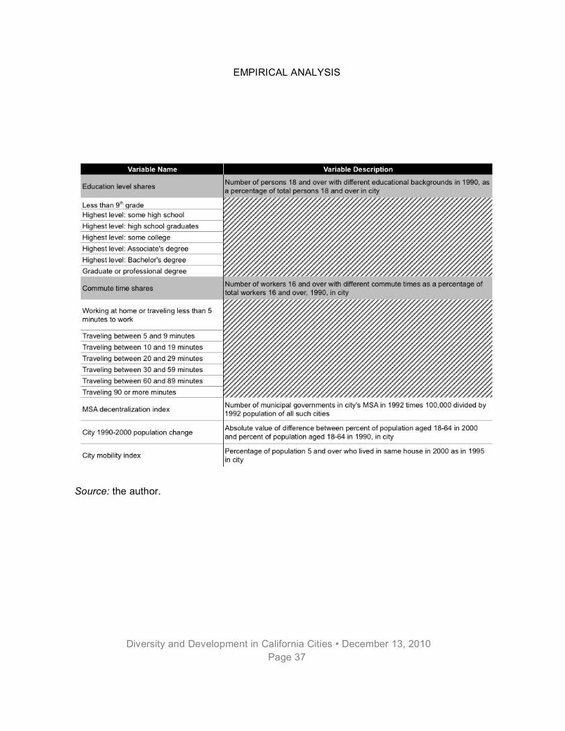
EMPIRICAL ANALYSIS


Source: the author.

EMPIRICAL ANALYSIS


Table IV-3. Descriptive Statistics for Variables Used in Analysis.

Note: This table continues on the next page.

EMPIRICAL ANALYSIS


Source: the author.

EMPIRICAL ANALYSIS


This sample represents the intersection of the cities described by the 1990 census, the 2000 census, and the 1992 Census of Governments.108 Those cities which fell outside MSAs in 1990 were excluded because of the attention paid in the literature to describing economic activity in MSAs.109

The dependent variable in all regressions is the change in median household income in the city between 1989 and 1999.

Figure IV-1. Frequency Distribution for Ethnic Diversity Variables.

Source: author’s calculations.

108 Three small cities would have otherwise been included because they met all three criteria listed in the text, but were excluded from the analysis. Please see the appendix for a list of those cities and an explanation of why they were excluded. 109 For examples of studies which look at economic activity within MSAs, see: Edward L. Glaeser, José A. Scheinkman, and Andrei Shleifer, “Economic Growth in a Cross-Section of Cities;” Gianmarco I.P. Ottaviano and Giovanni Peri, “Cities and Cultures;” and Dean Stansel, “Local decentralization and local economic growth: A cross-sectional examination of US metropolitan areas.” Note that, in the sample of 378, the dependent variable has a mean and standard deviation of $15,017 and $12,651 respectively. If cities outside MSAs were included, in that sample of 443, the mean and standard deviation of the dependent variable would be $14,086 and $10,097, respectively. Therefore, exclusion of non-MSA cities slightly raises the mean and standard deviation of the dependent variable.

EMPIRICAL ANALYSIS


Figure IV-2. Comparison of 1990 Ethnic Diversity Data Across Aggregation Levels.

Source: author’s manipulation of census data.110

The MSA level and city level variables differ in their means and variances. Mean values of the index are higher at the MSA level: the city-level ethnic SDI has a mean level of 0.37, while the MSA level SDI has a mean of 0.48. This is believed to happen as pockets of complementary low-diversity areas combine to form higher-diversity areas.111 In addition, the 110 See Figure I-1 for a more complete legend, which includes many map elements not included in the legend here. Also see the appendix for more details on how the tract-level figures were created. 111 A theoretical example is shown in order to illustrate what is believed to be happening. Suppose that G is equal to 2. If, at a lower level of geographic aggregation, group A makes up one-third of the population and group B two-thirds in city X, compared to the opposite in city Y (i.e., two-thirds group A and one-third group B). If we aggregate to the MSA level, where the MSA contains city X and city Y, the MSA will be split evenly between group A and group B, and therefore MSA-level diversity will be higher than city-level diversity.

EMPIRICAL ANALYSIS


variance is 0.03 for the city-level variable and 0.01 for the MSA-level variable. One can see in Figure IV-1 why this happens. As the aggregation becomes coarser, the extreme values of the SDI, shown at the edges of the blue curve, fade away, thus lowering the variance.

Figure IV-2 shows how the SDIs vary across spatial scales, measuring them at the census tract level compared to at the city level. One can see that when one looks at an area with more detail, there is more variation at the tract level. For example, Fresno appears to be uniformly high-diversity in Figure I-1, but in Figure IV-2, one can clearly see pockets of low diversity. This further illustrates the concept of how complementary areas combine to form higher diversity areas at higher levels of geographic aggregation.

C. Methods

The regression analysis is conducted in two phases. First, a base model is constructed, and then, a diversity model adds the various ethnic and linguistic variables that are of most concern.

1. Base Model

The Base Model uses city-level changes in median household income as the dependent variable. The variables shown in Table IV-3 were tested for their significance in a multiple regression framework, except that one variable from each of the three big categories (travel variables, education variables, and industry variables) were excluded for econometric reasons.112

The following refinements to the base model were made:

• Variables related to commute times were not significant and thus they were dropped from the model.

• Among the industry variables, six were significant—two positive and four negative. While there was no plausible explanation for each of the coefficients, shares by industry are a key feature of several studies cited in this report, and thus they stayed in the model.

• The vacancy rate, unemployment rate, and percent of the population receiving public assistance variables were removed from the model because of perceived multicollinearity with the above industry variables.

112 The first one in each group was excluded.

EMPIRICAL ANALYSIS


Table IV-4. Regression Results from Stansel and Glaeser et al.

Source: Glaeser et al.113 and Stansel.114

• The per capita government debt and per capita government revenue variables were dropped from the model because they were not significant. The expenditure variable remained because it is significant in some of the models presented.

Two versions of the base model are presented, one with the MSA decentralization variable, and one without. The version with this variable (Base Model 2) can be compared to 113 Edward L. Glaeser, José A. Scheinkman, and Andrei Shleifer, “Economic Growth in a Cross-Section of Cities.” Note that Glaeser et al. do not report a standard error on the constant term, which means that the significance of the constant is unknown. 114 Dean Stansel, “Local decentralization and local economic growth: A cross-sectional examination of US metropolitan areas.”

EMPIRICAL ANALYSIS


the regression results shown on the left side of Table IV-4, while the version without it (Base Model 1) can be compared to the results on the right side of Table IV-4.

2. Diversity Model

To Base Model 2, the four key diversity variables were added in individual regressions rather than combining them. Thus, the Diversity Model retains the dependent variable and explanatory variables from the Base Model, and adds to it measures of ethnic and linguistic diversity. With each of the four key independent variables, a squared term was tested, and was kept in the model if it added to the explanatory power of the model and was statistically significant.

3. Benefits of City-Level Analysis Over Smaller Scales

In designing the model, a decision was made about the spatial scale at which to measure the changes in income. Originally, the intent of the report was to look at the level of the census tracts and include in the model predictor variables for population diversity at three different scales: at the level of the census tract, city, and MSA. The use of the census tract as the unit of analysis was based on an earlier study which looked at economic impacts of heavy rail stations at this level.115 While sample sizes were significantly larger, results were weaker because of the prevalence of outlying data. Earlier versions of the model which looked at census tracts had adjusted R-squared values of below 0.30, significantly lower than those which are reported here.

For example, a census tract which housed a prison faced a 100% decrease in median household income, possibly because a change in the ratio of non-earners started to earners, or prisoners to staff. This kind of issue creates wide variation in data when examining it at a small scale—problems which need not be dealt with at the city level.

D. Hypotheses

It is hypothesized that population diversity has a positive effect on urban economic growth based on the finding that wages and rents are higher in the presence of cultural diversity. This is based on the view that factors which positively influence productivity should also positively influence urban economic growth. Therefore, it is hypothesized that the Diversity Model will provide an increase in the adjusted R-squared value above the Base Model, and that at least one of the population diversity variables in the Diversity model will be statistically significant.

Moreover, the spatial scale at which this effect is most pronounced, is hypothesized to be at the city level, meaning that the city-level diversity variables will be better predictors of 115 Christopher R. Bollinger and Keith R. Ihlanfeldt, “The Impact of Rail Transit on Economic Development: The Case of Atlanta’s MARTA,” Journal of Urban Economics 42, no. 2 (1997): 179-204.

EMPIRICAL ANALYSIS


city-level changes than will the MSA-level variables. The rationale behind this hypothesis is that people spend more of their time in their cities than in surrounding cities, and thus are most deeply affected by interactions in their home cities.116

E. Results

Results from the Base Models and Diversity Models are shown in Table IV-5.

1. Comparing Base Model 1 to Glaeser et al.

First, Base Model 1 is compared to column 5 of Table 10 in Glaeser et al.117 There are several key differences in the design of the two models:

• The model in this report includes shares for six industries, while Glaeser et al. present just one. Across the results, two industry sectors consistently have significant and positive coefficients (communications and other public utilities; and wholesale trade), while four have negative coefficients (finance, insurance, and real estate; entertainment and recreation services; health services; and education services).

• Glaeser et al. use geographical dummies depending on where in the country the city is located, which cannot be applied to this report.

• Instead of using several education variables showing the percentage of the population in each group, as done in this report, Glaeser et al. use median years of schooling instead.

• Glaeser et al. include the initial unemployment rate, a variable which was not included in this model for reasons discussed above.

• This report also includes two controls, discussed above, which do not appear in Glaeser et al.

Glaeser et al. also include two more variables showing initial population and initial income which do not appear here. The key similarity between the two sets of results are the significant and positive effect of education shown in both models. Across all the results, the highest education variable, the percent of the population with more than a bachelor degree, is highly significant and positively correlated with income growth.

The key difference between the two models is the sign of the per capita expenditure variable. Whereas in Glaeser, the coefficient is significant and positive, here it is significant

116 A significant limitation of this paper is that it cannot also focus on the population diversity which exists in the neighborhoods where people go to work. 117 Edward L. Glaeser, José A. Scheinkman, and Andrei Shleifer, “Economic Growth in a Cross-Section of Cities.”

EMPIRICAL ANALYSIS


and negative in Base Model 1. In other models, however, the variable loses its significance slightly.

The sample size is smaller in Glaeser et al. (201 compared to 378), and the adjusted R-squared is also smaller (0.44 compared to 0.62).

2. Comparing Base Model 2 to Stansel

Base Model 2 is compared to the third column in Stansel’s Table 3.118 Stansel displays an R-squared value of 0.719, compared to the 0.643 shown here. Stansel’s sample size (314) is more similar to the one used in this report. The key differences are as follows:

• As mentioned earlier, Stansel uses four decentralization variables showing the per capita number of different types of governments: public school systems, county governments, townships, and municipalities. Whereas Stansel finds the municipal variable is positively correlated and significant at a 95% level, Base Model 2 shows the MSA decentralization index’s coefficient to be significant and negative.

• Stansel includes several variables not included in Base Model 2, like population growth in the period preceding the period under consideration, initial population, initial income, and the initial manufacturing share. Base Model 2 uses several industry shares and per capita expenditure variables which Stansel does not use.

• Stansel’s only education variable, the percent of the population with 16 or more years of school, has a positive sign, but it is not significant.

3. Diversity Model Results

The Diversity Models add to the Base Models various diversity variables, which are all negatively signed, and which add a very small amount to the adjusted R-squared value. In the four models, the adjusted R-squared rises between 0.003 and 0.017. For example, it goes up from 0.627 in Base Model 2 to 0.634 in the City Ethnic Diversity Model. The largest increase is in the MSA Linguistic Diversity Model, as shown in Table IV-5.

118 Dean Stansel, “Local decentralization and local economic growth: A cross-sectional examination of US metropolitan areas.”

EMPIRICAL ANALYSIS


Table IV-5. Base Model and Diversity Model Results.

Source: author’s analysis.

EMPIRICAL ANALYSIS


In all four Diversity Models, the diversity variables are significantly negatively correlated with the dependent variable. Nevertheless, the negative sign on the ethnic diversity variable is significant at the 95% level. The interpretation of the coefficient makes the most sense when discussing changes at the level of one-tenth of a point: an increase of 0.1 in the ethnic diversity index led to a decrease in median household incomes in the city of $628.

The most significant coefficient is in the MSA Linguistic Diversity Model. In the City Linguistic Diversity Model, the coefficient is significant at the 90% level while in the other three, it is significant at the 95% level. Therefore, the coefficients are significant and add to the explanatory power of the model, but their coefficient is opposite from the expectation.

In order to delve more deeply into the relationship between the diversity variables and the dependent variable, squared terms were introduced. For the most part, these did not add to the explanatory power of the models, and in fact took away from the significance which had been held by the unsquared terms alone. However, the square of the MSA-level ethnic diversity variable was significant, and added to the adjusted R-squared, which is why it is included in a model.

The positive coefficient on the un-squared term and a negative coefficient on the squared term suggests a hill-shaped curve relationship. This relationship was further analyzed by dividing the sample of 378 into three groups and comparing the mean value of the dependent variable, rawincCH, across groups, as shown in Table IV-6. In the middle group group, the mean value of the dependent variable higher than in both the low and high groups. This is evidence of an ideal range of MSA-level ethnic diversity, where if it is too high or too low, growth is lower.

Table IV-6. Description of Three Groups Separated by MSA Ethnic Diversity Value.

Source: author’s calculations.

The expectation about which scale is best for measuring diversity appears to have been wrong. While the adjusted R-squared of the City Ethnic Diversity Model is the same as the MSA Ethnic Diversity Model, the MSA Linguistic Diversity Model is a little higher than the

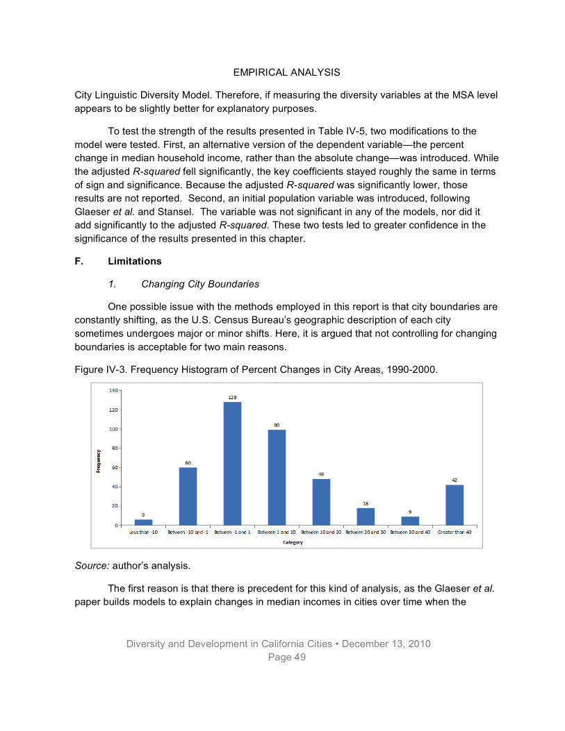
EMPIRICAL ANALYSIS


City Linguistic Diversity Model. Therefore, if measuring the diversity variables at the MSA level appears to be slightly better for explanatory purposes.

To test the strength of the results presented in Table IV-5, two modifications to the model were tested. First, an alternative version of the dependent variable—the percent change in median household income, rather than the absolute change—was introduced. While the adjusted R-squared fell significantly, the key coefficients stayed roughly the same in terms of sign and significance. Because the adjusted R-squared was significantly lower, those results are not reported. Second, an initial population variable was introduced, following Glaeser et al. and Stansel. The variable was not significant in any of the models, nor did it add significantly to the adjusted R-squared. These two tests led to greater confidence in the significance of the results presented in this chapter.

F. Limitations

1. Changing City Boundaries

One possible issue with the methods employed in this report is that city boundaries are constantly shifting, as the U.S. Census Bureau’s geographic description of each city sometimes undergoes major or minor shifts. Here, it is argued that not controlling for changing boundaries is acceptable for two main reasons.

Figure IV-3. Frequency Histogram of Percent Changes in City Areas, 1990-2000.

Source: author’s analysis.

The first reason is that there is precedent for this kind of analysis, as the Glaeser et al. paper builds models to explain changes in median incomes in cities over time when the

EMPIRICAL ANALYSIS


boundaries of those cities are shifting.119 They argue that such methods are justified because they build similar models to explain changes in median incomes at broader MSA levels and find that the predictor variables produce similar coefficients across the two kinds of analysis.

The second reason is that the large majority of cities in the analysis underwent small changes in their areas during the 1990s, relative to their 1990 areas. This is clear from Figure IV-3, which shows that the large majority of the cities in the sample underwent somewhere between a -10% and 20% change in their areas during the time period.

The third reason why it is reasonable to downplay this issue is that the percent change in area does not appear to be correlated in an empirical sense with either the key dependent variables or the key predictor variables in this analysis. Regression results, included as an appendix, showed that there was not a strong relationship between the variables in question.

2. Changing Sets of Cities

By studying the intersection (and not the union) of 1992 Census of Governments datasets, 1990 decennial census datasets, and 2000 decennial census datasets, the full dynamics of urban growth may not be considered. In other words, there is growth occurring in areas which were not cities in one of those three datasets.

To analyze this limitation, the sets of cities which existed in the 1992 and 2002 Census of Governments files were analyzed. Only 3.7% of the cities which existed in 1992 ceased to exist under their 1992 names over that period, while 6.5% of the cities which existed in 2002 had not existed in 1992.

3. Changing MSA Definitions

Finally, there is a potential issue with measuring MSA-level population diversity in 1990 when MSA boundaries shifted over the course of the 1990s. This report investigates the effect of MSA-level diversity because MSAs are drawn to take into account where people work, instead of simply where they live. Because MSA boundaries shifted, one can imagine a problem because 1990 boundaries do not describe 1999 commute patterns as well as the 2000 boundaries do.

In order to assess this issue, the extent of changes in MSA boundaries was examined. Whereas Yolo County and Sacramento County were one MSA in 1990, they split in 2000 to become two MSAs. Of the 16 cities which were in the Sacramento MSA in 1990, four ended up being in the Yolo MSA in 2000. Therefore, 16 cities, or 4.2% of the sample, show a value of the MSA-level variable which is different than if it were to be calculated using 2000 MSA boundaries.

119 Ibid.

V. CONCLUSIONS

A. Lessons Learned from Empirical Analysis

The results show a small but noticeable negative relationship between 1990 population diversity and 1990-2000 growth in city median household income. Therefore, there was no support found for the hypothesis that income changes would be positively correlated with population diversity, while there was support for the hypothesis that the population diversity variables would contribute to the adjusted R-squared value. Meanwhile, there was also no support for the hypothesis that the effect of the diversity variables would be more significant at the city-level than at the MSA-level.

For the most part, the relationship between diversity and changes in income was determined to be linear and negative: more diversity resulted in lower growth. However, with the MSA-level diversity variable, a different pattern emerges. The Empirical Analysis chapter provides evidence that there is an optimal range for MSA-level ethnic diversity, where if MSAs become too high or too low, growth suffers.

Constructing this model allowed for some investigation as to what the optimal spatial scale is for investigating the causes of changes in median household income. This report makes the determination that conducting a city-level analysis is the best method. There are several limitations discussed above, like the changing boundary problem, but none is so significant to discount the results presented in this report. The main lesson learned from having considered different spatial scales is that none of the spatial scales is perfect in every way.

B. Contributions to Existing Literature

The results provide an opportunity to reflect on the merits of various theories used to explain the relationship between economic growth and population diversity. The literature review highlighted contradictory views about the nature of this relationship: some arguments held that the consumption benefits associated with population diversity would lead to higher growth, while others held that higher transaction costs and inter-group conflicts would lower prospects for growth. Because a negative effect of ethnic diversity has been observed in the context of 1990s California, it is supposed that within this context where the theories have been tested, the negative arguments outweigh the positive ones.

The primary predictor of the changes in median household income was related to educational attainment, as demonstrated by the relatively large coefficient on the variable representing the percentage of people who have completed graduate-level education. This is a result that supports previous findings as to the key determinants of urban growth, like in

CONCLUSIONS


Glaeser et al.120 However, findings related to the per capita number of municipal governments and per capita municipal expenditures run counter to the existing literature, which perhaps suggests that these topics need to be revisited.

A key claim that this report investigates is that the trends which affect productivity at a given time will likewise affect economic growth. In other words, the reason why this report looks at population diversity as a potential predictor of urban economic growth was that Ottaviano and Peri argued that it positively affects productivity as measured instantaneously.121 This argument appears not to have much validity based on the results. Rather, if anything, the negative impacts of population diversity, which are widely discussed in the international studies on growth, appear to emerge in California.

C. Future Directions and Implications for Planners

Future work could delve more deeply into the relationship between diversity and development by testing the validity of the theoretical concepts which were discussed in the Literature Review. For example, standardization of consumption spaces is cited as a factor which could mute the positive effects of ethnic diversity. With that in mind, it would be useful to include a variable which captures this standardization (e.g., the number of McDonald’s restaurants) or the lack thereof (e.g., the number of establishments selling ethnic cuisine). Likewise, data could be used to operationalize the key concepts of higher transactional costs and inter-ethnic conflict, which are hypothesized to be the channel through which population diversity lowers growth. For example, one might obtain data on the linguistic isolation and geographical proximity of nearby populations, or the frequency of crimes that can be described as inter-ethnic conflict. Such data can provide a more detailed description of the mechanism through which diversity impacts development.

Another future direction is to explore the ways in which levels of face-to-face contact affect this relationship between diversity and development. As discussed in the Literature Review, some researchers believe that people are now spending less time interacting with other people directly, and spend more time interacting with technology which makes place irrelevant.122 If place is less relevant, so too should be the theories which relate population diversity to growth. Therefore, if one can operationalize levels of face-to-face contact, or lack thereof, and create an interaction term with levels of population diversity, one could analyze the effect of population diversity in places with high face-to-face contact versus low face-to-face contact. This approach could potentially add to the explanatory power of the models described in this report.

120 Edward L. Glaeser, José A. Scheinkman, and Andrei Shleifer, “Economic Growth in a Cross-Section of Cities.” 121 Gianmarco I.P. Ottaviano and Giovanni Peri, “Cities and Cultures.” 122 Michael Storper and Anthony J. Venables, “Buzz: Face-to-Face Contact and the Urban Economy.”

CONCLUSIONS


While a negative relationship has been observed for the key relationship in question, the result is not so significant that it should cause a restructuring of planning efforts. However, the results do suggest that the strategies pursued in Calgary and Baltimore, which were discussed in the Introduction, may not be the best way to plan for economic growth. Meanwhile, because the theories suggesting a negative relationship relate to higher transaction costs and the potential for inter-group conflict, the role of the planner should be to mediate disputes and lower transaction costs wherever possible. This involves active community engagement so that stakeholders from different ethnic groups are brought to the negotiating table to facilitate discussion about the city’s future. At the same time, planners and policymakers should continue to embrace the positive impacts of population diversity which are observed in the literature, like the wealth of consumption and production opportunities that it presents.

CONCLUSIONS


VI. BIBLIOGRAPHY

Alesksy-Szucsich, Agnieszka. Economic Benefits of Ethnolinguistic Diversity: Implications for International Political Economy. Amherst, NY: Cambria Press, 2008.

Alesina, Alberto, Arnaud Devleeschauwer, William Easterly, Sergio Kurlat, and Romain Wacziarg. “Fractionalization.” Journal of Economic Growth 8, no. 2 (2003): 155-94.

Alesina, Alberto, and Eliana La Ferrara. “Ethnic Diversity and Economic Performance.” Journal of Economic Literature 43, no. 3 (2005): 762-800.

Alesina, Alberto, Reza Baqir, and William Easterly. “Public Goods and Ethnic Divisions.” Quarterly Journal of Economics 114, no. 4 (1999): 1243-84.

Aydemir, Abdurrahman, and George J. Borjas. “Cross-Country Variation in the Impact of International Migration: Canada, Mexico, and the United States.” Journal of the European Economic Association 5, no. 4 (2007): 663-708.

Bollinger, Christopher R., Keith R. Ihlanfeldt. “The Impact of Rail Transit on Economic Development: The Case of Atlanta’s MARTA.” Journal of Urban Economics 42, no. 2 (1997): 179-204.

Borjas, George J. “Self-Selection and the Earnings of Immigrants.” American Economic Review 77, no. 4 (1987): 531-53.

Campbell, Donald T. “Blind Variation and Selective Retention in Creative Thought as in Other Knowledge Processes.” Psychological Review 67, no. 6 (1960): 380-400.

Caselli, Francesco, and Wilbur John Coleman II. “On the Theory of Ethnic Conflict.” Discussion Paper #732, Centre for Economic Performance, 2006.

Cheshire, Paul, and G. Carbonaro, “Urban Economic Growth in Europe: Testing Theory and Policy Prescriptions.” Urban Studies 33, no. 7 (1996): 1111-28.

Dixit, Avinash K., and Joseph E. Stiglitz. “Market Competition and Optimum Product Diversity.” American Economic Review 67, no. 3 (1977): 297-308.

Easterly, William, and Ross Levine. “Africa’s Growth Tragedy: Policies and Ethnic Divisions.” Quarterly Journal of Economics 112, no. 4 (1997): 1203-50.

Fischel, William. “Zoning and the Exercise of Monopoly Power: a Reevaluation.” Journal of Urban Economics 8, no. 3 (1980): 283-93.

Florida, Richard. Rise of the Creative Class. New York: Basic Books, 2002.

Galor, Oded, and Quamrul Ashraf. “Cultural Assimilation, Cultural Diffusion and the Origin of the Wealth of Nations.” Discussion Paper #DP6444, Centre for Economic Policy Research, 2007.

Glaeser, Edward L., Hedi D. Kallal, José A. Scheinkman, and Andrei Shleifer. “Growth in Cities.” Journal of Political Economy 100, no. 6 (1992): 1126-52.


Glaeser, Edward L., Jed Kolko, and Albert Saiz. “Consumer City.” Journal of Economic Geography 1, no. 1 (2001): 27-50.

Glaeser, Edward, and José A. Scheinkman. “Non-Market Interactions.” Working Paper #8053, National Bureau of Economic Research, 2000.

Glaeser, Edward L., José A. Scheinkman, and Andrei Shleifer. “Economic Growth in a Cross-Section of Cities.” Journal of Monetary Economics 36, no. 1 (1995): 117-43.

Knack, Stephen, and Philip Keefer. “Does Social Capital Have an Economic Payoff? A Cross-Country Investigation.” Quarterly Journal of Economics 112, no. 4 (1997): 1251-88.

Lazear, Edward P. “Culture and Language.” Journal of Political Economy 107, no. 6 (1999): 95-125.

Macpherson, David A., and G. Stacy Sirmans. “Neighborhood Diversity and House-Price Appreciation.” Journal of Real Estate Finance and Economics 22, no. 1 (2001): 81-97.

Maignan, Carole, Gianmarco Ottaviano, Dino Pelli, and Francesco Rullani. “Bio-Ecological Diversity vs. Socio-Economic Diversity: A Comparison of Existing Measures.” Working Paper #13.2003, Fondazione Eni Enrico Mattei, 2003.

Montalvo, Jose G., and Marta Reynal-Querol. “Ethnic Diversity and Economic Development.” Journal of Development Economics 76, no. 2 (2005): 293-323.

Murata, Yasusada. “Product Diversity, Taste Heterogeneity, and Geographic Distribution of Economic Activities: Market vs. Non-market Interactions.” Journal of Urban Economics 53, no. 1 (2003): 126-44.

Okten, Cagla, and Una Okonkwo Osili. “Contributions in Heterogeneous Communities: Evidence from Indonesia.” Journal of Population Economics 17, no. 4 (2004): 603-26.

Ottaviano, Gianmarco I.P., and Giovanni Peri. “The Economic Value of Cultural Diversity: Evidence from US Cities.” Journal of Economic Geography 6, no. 1 (2006): 9-44.

———. “Cities and Cultures.” Journal of Urban Economics 58, no. 2 (2005): 304-37.

———. “Rethinking the Gains from Immigration: Theory and Evidence from the US.” Working Paper #11672, National Bureau of Economic Research, 2005.

Quigley, John M. “Urban Diversity and Economic Growth.” The Journal of Economic Perspectives 12, no. 2 (1998): 127-38.

Saiz, Albert. “Immigration and Housing Rents in American Cities.” Journal of Urban Economics 61, no. 2 (2007): 345-71.

Scott, Allen J. “The Cultural Economy of Cities.” International Journal of Urban and Regional Research 21, no. 2 (1997): 323-39.


Sparber, Chad. “A Theory of Racial Diversity, Segregation, and Productivity.” Journal of Development Economics 87, no. 2 (2008): 210-26.

———. “Racial Diversity and Economic Productivity—Industry Level Evidence.” Manuscript, University of California, Davis, 2005.

———. “Racial Diversity and Macroeconomic Productivity Across US States and Cities.” Working Paper, University of California, Davis, 2006.

Stansel, Dean. “Local decentralization and local economic growth: A cross-sectional examination of US metropolitan areas.” Journal of Urban Economics 57, no. 1 (2005): 55-72.

Storper, Michael, and Anthony J. Venables. “Buzz: Face-to-Face Contact and the Urban Economy.” Journal of Economic Geography 4, no. 4 (2004): 351-70.

Tajfel, Henri, M.G. Billig, R.P. Bundy, and Claude Flament. “Social Categorization and Intergroup Behaviour.” European Journal of Social Psychology 1, no. 2 (1971): 149-78.

Uslaner, Eric. “Does Diversity Drive Down Trust?” Working Paper 69.2006, Fondazione Eni Enrico Mattei, April 2006.

Zukin, Sharon. “Urban Lifestyles: Diversity and Standardisation in Spaces of Consumption.” Urban Studies 35, no. 5-6 (1998): 825-39.



APPENDICES

1. Map Production

The US Census produces cartographic boundary files for places in California.123 Just those cities which are included in the sample were displayed in Figure I-1 and Figure I-2. The sample includes cities which appear in the 1990 census, 2000 census, and 2002 Census of Governments—and only those cities which fall inside 1990 MSA boundaries. The maps apply quantitative data from the 1990 decennial census to 1990 census boundary files.

Figure IV-2 was also created using the same kind of ethnic diversity data from the 1990 census, but with different geography. Here, the set of areas is defined by the clipping of the 1990 census tract boundary file by the 1990 place boundary file. If a tract lay on both sides of a place boundary, only the part of the tract which falls inside the place boundary was retained. Those tracts, or pieces of tracts, which remained were kept as areas to be displayed, regardless of whether they appeared in the 1992 Census of Governments or 2000 decennial census. This means that some areas are shown in Figure IV-2 but not the other two maps.

Census boundary files have a field which displayed the city’s Federal Information Processing Standard (FIPS) code. This field was used to join the attribute data from American FactFinder.124 In ArcGIS, two separate layer files were then created: one where symbology was applied based on the value of the ethnic diversity index, and the other which used the linguistic diversity index. In all cases, the same five colors were applied by establishing quintiles and rounding the break points to the nearest 0.01. Different layers were then applied to different data frames.

Some more metadata is available on the source and currency of the maps’ layers. The US Census created shapefiles for places and counties in 2001. Boundaries of other states (e.g., Oregon and Nevada) and of Mexico were created by the makers of GIS Tutorial: Workbook for ArcView 9 in 2007.125 Also, the interstates on the map come from a 2001 layer showing state highways created by Caltrans.126 Only those segments where the functional class (variable FUNCCL) equals 1 and 11—rural and urban interstates—are shown. All of these layers were projected using the NAD 1983 California Teale Albers projection coordinate system.

123 These include cities, towns, and census-designated places. 124 U.S. Census, “American FactFinder,” http://factfinder.census.gov/home/saff/main.html?_lang=en (accessed November 20, 2009). 125 Wilpen L. Gorr and Kristen S. Kurland, GIS Tutorial: Workbook for ArcView 9 (Redlands, CA: ESRI Press, 2008), enclosed CD. 126 The highways layer was obtained from an FTP at svctftp.dot.ca.gov with login information provided by a Caltrans employee.


2. Why Certain Cities Were Excluded

The cities of Vernon, Irwindale, and Industry were excluded from the analysis since they are essentially industrial areas rather than typical cities. The three of them have by far the highest per capita tax levels of any of the cities in the sample, with Industry at $91,000, Vernon at $57,000, and Irwindale at $22,000. The next highest per capita tax levels are under $8,000. Moreover, these three also had the top three per capita revenue levels.

In addition, five cities (Temecula, Dana Point, Yucaipa, Laguna Niguel, and Diamond Bar) were included in the original 1992 Census of Governments file but all of the values were filled in as zeroes. The likely explanation for this is that all five of these cities had recently incorporated in 1989, and that is why these cities were not included in the sample used in this analysis.

3. Census Variable Codes Used

Appendix Table 1 includes a complete list of the sources of census variables.

Appendix Table 1. Census Variables Used.

Source: U.S. Census Bureau variables.

4. Why the Area-Related Control Was Excluded

This section addresses the issue of why the model employed in this report does not include a control variable which accounts for percent changes in area. For all of the


municipalities in the sample, using U.S. Census geography,127 the area of all cities in the sample were obtained for 1990 and 2000, and using that data, a variable for the percent change in area was calculated. A histogram for that variable is shown in Figure IV-3, and as discussed within the main body of the report, the majority of the changes are within -10% and 20%.

Furthermore, as shown in Appendix Table 2, the inclusion of the control variable results in very small (less than 1%) changes in the standardized coefficients of the key population diversity variables:

Appendix Table 2. Sensitivity of Key Coefficients to Change-in-Area Control Variable.

Source: author’s analysis of census data.

If the control were somehow affecting the relationships of the key variables being studied, its inclusion in the model would be justified. But here, the impact is very insignificant.

Finally, the relationship between the main dependent variable (rawincCH) and the area control variable was considered. One hypothesis that was considered was that cities which expanded more were likely to attract investment in the process of growing, and therefore we should observe a positive correlation between the control and the dependent variable. Yet, the observed correlation between the two was extremely weak. The adjusted R-squared value was very low (0.004), and the coefficient was almost significant (a p-value of 0.104), but negative. These observations suggest that there is probably no link between the two variables, and even more likely, the link is not as hypothesized.

5. MSA-Level Values of the Diversity Variables

The following table includes the values of the MSA-level ethnic and linguistic diversity variables across all PMSAs (Primary Metropolitan Statistical Areas) and MSAs in California:

127 U.S. Census, “Cartographic Boundary Files,” http://www.census.gov/geo/www/cob/bdy_files.html (accessed September 25, 2010).


Appendix Table 3. Values of MSA-Level Diversity Variables Across all MSAs.

Source: author’s manipulation of decennial census data.

Documents

DIVERSITY AND DEVELOPMENT IN CALIFORNIA CITIES€¦ · 100% sample of responses to the short form questions on the 1990 census, while the language variable is based on a roughly 1-in-7