Diversity and Composition of Demersal Fishes along a Depth

Diversity and Composition of Demersal Fishes along aDepth Gradient Assessed by Baited Remote UnderwaterStereo-VideoVincent Zintzen1*, Marti J. Anderson2, Clive D. Roberts1, Euan S. Harvey3, Andrew L. Stewart1,

Carl D. Struthers1

1 Museum of New Zealand Te Papa Tongarewa, Wellington, New Zealand, 2 New Zealand Institute for Advanced Study, Massey University, Albany Campus, Auckland, New

Zealand, 3 School of Plant Biology and University of Western Australia Oceans Institute, University of Western Australia, Crawley, Western Australia, Australia

Abstract

Background: Continental slopes are among the steepest environmental gradients on earth. However, they still lack finerquantification and characterisation of their faunal diversity patterns for many parts of the world.

Methodology/Principal Findings: Changes in fish community structure and diversity along a depth gradient from 50 to1200 m were studied from replicated stereo baited remote underwater video deployments within each of seven depthzones at three locations in north-eastern New Zealand. Strong, but gradual turnover in the identities of species andcommunity structure was observed with increasing depth. Species richness peaked in shallow depths, followed by adecrease beyond 100 m to a stable average value from 700 to 1200 m. Evenness increased to 700 m depth, followed by adecrease to 1200 m. Average taxonomic distinctness g+ response was unimodal with a peak at 300 m. The variation intaxonomic distinctness L+ first decreased sharply from 50 to 300 m, then increased beyond 500 m depth, indicating thatspecies from deep samples belonged to more distant taxonomic groups than those from shallow samples. Fishes withnorthern distributions progressively decreased in their proportional representation with depth whereas those withwidespread distributions increased.

Conclusions/Significance: This study provides the first characterization of diversity patterns for bait-attracted fish specieson continental slopes in New Zealand and is an imperative primary step towards development of explanatory and predictiveecological models, as well as being fundamental for the implementation of efficient management and conservationstrategies for fishery resources.

Citation: Zintzen V, Anderson MJ, Roberts CD, Harvey ES, Stewart AL, et al. (2012) Diversity and Composition of Demersal Fishes along a Depth Gradient Assessedby Baited Remote Underwater Stereo-Video. PLoS ONE 7(10): e48522. doi:10.1371/journal.pone.0048522

Editor: Brian R. MacKenzie, Technical University of Denmark, Denmark

Received June 10, 2012; Accepted September 26, 2012; Published October 31, 2012

Copyright: � 2012 Zintzen et al. This is an open-access article distributed under the terms of the Creative Commons Attribution License, which permitsunrestricted use, distribution, and reproduction in any medium, provided the original author and source are credited.

Funding: This work was supported by a Royal Society of New Zealand Marsden grant (MAU0713), Te Papa Collection Development Programme (AP3126) andFoundation for Research, Science and Technology/National Institute of Water and Atmospheric Research Marine Biodiversity and Biosecurity OBI (contractCOIX0502). The funders had no role in study design, data collection and analysis, decision to publish, or preparation of the manuscript.

Competing Interests: The authors have declared that no competing interests exist.

* E-mail: [email protected]

Introduction

Continental slopes extend from the outer edge of the continental

shelf (,100–200 m depth) to the base of the slope (,4000 m)

where abyssal plains begin. They are among the steepest

environmental gradients on earth. Factors such as light, hydro-

static pressure, temperature, oxygen concentration, food availabil-

ity, nature of water masses and substrate type all drastically change

within a few hundred meters. The fauna are also known to change

along this depth gradient. The fact that species composition

changes with depth, resulting in distinct identifiable communities

associated with the shelf, slope and abyssal plain has been virtually

unchallenged since the 1970’s [1], but finer quantification and

characterisation of such patterns for many parts of the world are

still lacking. Diversity is increasingly acknowledged as essential for

ecosystem functioning and the provision of goods and services to

humanity [2,3,4,5]. There has been relatively little work done,

however, to understand the potential role of biodiversity for

maintaining resilience and sustainability in marine ecosystems,

compared to terrestrial or freshwater systems [6]. Elucidating

patterns in bathymetric diversity is also important in order to

complement our understanding of other known globally significant

gradients of biodiversity, such as latitudinal or altitudinal gradients

[7]. Understanding the mechanisms that control spatial variation

in species richness may improve predictions of how biodiversity

will respond to environmental changes and help the design of

effective conservation strategies [8]. However, the causes under-

lying faunal turnover and diversity patterns on continental slopes

have not been clearly identified [1]. A crucial first step is to

accurately document how communities change along depth

gradients.

Fishes, which account for more than half of all living vertebrates

[9], are an important component of slope and shelf communities,

particularly through their feeding activity which can regulate

trophic structure, and thus influence the stability and resilience of

PLOS ONE | www.plosone.org 1 October 2012 | Volume 7 | Issue 10 | e48522

populations and food-web dynamics in aquatic ecosystems [10,11].

Fisheries on continental margins also provide a significant amount

of protein to the world’s human populations [12]. However, most

fishes are highly mobile and therefore are difficult to sample,

especially in topographically complex or deep habitats. Assessing

the diversity of fishes on continental margins can be difficult

because of the heterogeneity of potential habitats [13], variation in

behaviour or abundances in the wild [14], and also because of the

selectivity of particular fishing gear towards particular species

[15,16] or inevitable biases inherent in the use of remotely

operated vehicles or submersibles [17,18], which tend not to be

deployed according to any structured sampling designs. In

addition, sampling at and beyond the shelf break (often at depths

beyond 200 m) is typically plagued with low levels of replication

imposed by technical constraints [19], which significantly

decreases the scope for potential inferences regarding patterns in

diversity. In this context, baited remote underwater stereo-video

system (stereo-BRUVs) deployments provide an extremely useful

method to obtain standardized samples of fish communities which

is non-destructive (unlike trawls) and can be easily replicated

within a spatially structured sampling design for rigorous

inferences [20].

It has been stated that the greatest diversity of marine species is

found at some intermediate depth on the continental slope [21].

However, this is still debated, with numerous studies yielding

inconsistent results for particular groups of organisms or locations

[22]. Potential causal explanations for the observed patterns are

also numerous, including the presence of oxygen minimum zones,

changes in sediment grain size, topographic complexity, the degree

of physical disturbance [23] or spatial and temporal variation in

food availability [24,25]. For example, Tolimieri [26] observed

decreasing species richness of groundfish assemblages on the

continental slope of the U.S. Pacific coast with increasing depth,

reaching a minimum at about 600–900 m, followed by a slight

increase. A similar pattern was observed for evenness [26]. In

other studies, species richness of fishes on continental slopes either

decreased continuously with depth [27,28,29], or showed a peak at

some intermediate depth [30,31]. The evenness of demersal fish

assemblages was also found to decrease with depth down to 500 m

in the northeast Atlantic [32].

Species diversity is often defined as the variety (richness) and

relative abundance (dominance pattern or evenness) of species in a

defined unit of study [33]. Relative abundances can also reflect the

distribution of traits in a community, which in turn can indicate

the strength and sign of intra-specific and inter-specific interac-

tions [34]. The concept of diversity is, however, not limited to

species richness and evenness. It can also include quantification of

endemism [35], biogeographic distributions of species [36],

information on the evolutionary history of the considered taxa

(i.e., their phylogeny) or the functional behaviour or life-history

characteristics of species [37]. For example, taxonomic distinctness

quantifies the relatedness of species within a sample, based on the

distance between species in a classification tree [38] and is used to

evaluate the taxonomic diversity of a sample. The average

taxonomic distinctness (AvTD) of a sample is defined as the

average path-length between all pairs of species through a Linnean

taxonomic tree. The variation in taxonomic distinctness (VarTD,

[39]) is a measure of how variable the path-lengths are among

species; it reflects the unevenness of the taxonomic tree for a given

sample. There has been relatively little work on how taxonomic

distinctness of fish assemblages changes with depth. On the

continental slope of the U.S. Pacific coast, AvTD has been shown

to be highest at approximately 500 m and lowest around 200 m,

while VarTD slightly increased to 200–300 m depth, then sharply

decreased at deeper depths [40]. This pattern was largely driven

by high diversity of Chondrichthyes at 500 m compared to

shallower or deeper strata. Off the coast of Corsica (Mediterra-

nean Sea), the AvTD was higher on the continental shelf (60–

120 m) than it was at deeper depths (250–570 m) where it was

more stable [41], and the VarTD was lower on the upper slope

(250–400 m) than on the continental shelf and lower slope (400–

570 m). Zintzen et al. [42] showed no relationship with depth for

AvTD, but found an increase in VarTD with depth in the

Southwest pacific Basin (from 0 to ,2000 m). This result indicated

that clusters of species within specialized (unrelated) families occur

at depth.

In this paper, we describe for the first time the fundamental

changes in fish community structure and diversity along a depth

gradient from 50 m to 1200 m, as obtained from replicated (n = 6)

Baited Remote Underwater Stereo-Video (stereo-BRUVs) deploy-

ments within each of seven depth zones at each of three locations

in north-eastern New Zealand. We hypothesized that: (1) changes

in community structure would be very strongly affected by depth,

and less affected by differences in locations; (2) diversity as richness

would peak at some intermediate depth, where a variety of habitat

conditions and thus fish adaptations to them overlap (3) evenness

would increase with depth, as surface waters tend to have higher

productivity that could lead to dominance in temperate waters; (4)

average taxonomic distinctness would remain stable with depth as

there is no expectation that groups of fishes with particular

phylogenetic traits or histories would have colonized restricted

zones of the continental slopes; (5) variation in taxonomic

distinctness would increase with depth, showing diversification of

species occurring only within specific groups; and (6) there would

be decreased endemism at deeper depths, where potential

connectivity is higher due to more uniform environmental

conditions.

Materials and Methods

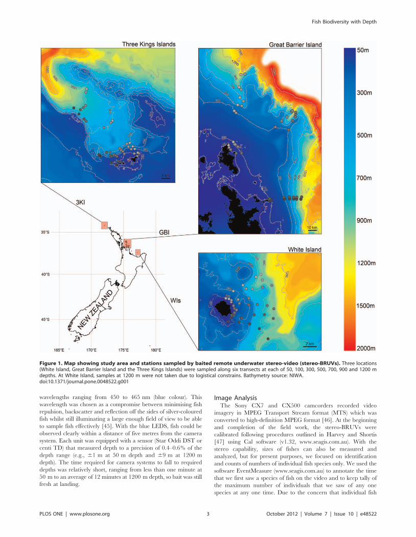
Location and Sampling MethodStereo-video footage was collected between March 2009 and

April 2010 at three locations, White Island (WI), Great Barrier

Island (GBI) and the Three Kings Islands (TKI), in the north of

New Zealand (Figure 1). At each location, video samples were

taken along each of six replicate transects during daylight hours,

and there were seven depth strata sampled per transect: 50, 100,

300, 500, 700, 900 and 1200 m, with the exception of WI where

we could not sample the 1200 m depth stratum, due to logistical

constraints. The resulting dataset comprised a total of 120 samples:

36 for WI (6 transects66 depth strata), 42 for GBI (6 transects67

depth strata) and 42 for TKI (6 transects67 depth strata). Each

deployment was located at least 500 metres away from any others

in order to minimise the probability of a fish visiting the bait at one

camera also being recorded by a neighbouring camera [43]. Each

deployment was treated as an independent replicate and was

deployed on the seabed for a minimum of two hours.

Seven separate stereo baited remote underwater stereo-video

systems (stereo-BRUVs) were used for deployments, having a

design adapted from the system used in shallow water by Harvey

et al. [44] to work at greater depth. Two HD Sony handycams

(models HDR-CX7 and HDR-CX500) were mounted on a stereo

configuration, 0.7 m apart on a base bar inwardly converged at 8uto gain an optimised field of view. The bait consisted of two

kilograms of Sardinops sagax (Jenyns 1842) that were thawed and

chopped prior to distribution into two bait bags visible in the field

of view. Lighting was provided by eight Royal Blue Cree XLamps

XP-E LEDs, each delivering a radiant flux of 350–425 mW at

Fish Biodiversity with Depth


wavelengths ranging from 450 to 465 nm (blue colour). This

wavelength was chosen as a compromise between minimising fish

repulsion, backscatter and reflection off the sides of silver-coloured

fish whilst still illuminating a large enough field of view to be able

to sample fish effectively [45]. With the blue LEDS, fish could be

observed clearly within a distance of five metres from the camera

system. Each unit was equipped with a sensor (Star Oddi DST or

centi TD) that measured depth to a precision of 0.4–0.6% of the

depth range (e.g., 61 m at 50 m depth and 69 m at 1200 m

depth). The time required for camera systems to fall to required

depths was relatively short, ranging from less than one minute at

50 m to an average of 12 minutes at 1200 m depth, so bait was still

fresh at landing.

Image AnalysisThe Sony CX7 and CX500 camcorders recorded video

imagery in MPEG Transport Stream format (MTS) which was

converted to high-definition MPEG format [46]. At the beginning

and completion of the field work, the stereo-BRUVs were

calibrated following procedures outlined in Harvey and Shortis

[47] using Cal software (v1.32, www.seagis.com.au). With the

stereo capability, sizes of fishes can also be measured and

analyzed, but for present purposes, we focused on identification

and counts of numbers of individual fish species only. We used the

software EventMeasure (www.seagis.com.au) to annotate the time

that we first saw a species of fish on the video and to keep tally of

the maximum number of individuals that we saw of any one

species at any one time. Due to the concern that individual fish

Figure 1. Map showing study area and stations sampled by baited remote underwater stereo-video (stereo-BRUVs). Three locations(White Island, Great Barrier Island and the Three Kings Islands) were sampled along six transects at each of 50, 100, 300, 500, 700, 900 and 1200 mdepths. At White Island, samples at 1200 m were not taken due to logistical constrains. Bathymetry source: NIWA.doi:10.1371/journal.pone.0048522.g001



may be counted repeatedly upon leaving and re-entering the field

of view over the two-hour period of sampling, the maximum

number of individuals of the same species appearing at the same

time (MaxN, [48]) was used as a conservative estimate of the

number of fish seen of any one species from each stereo-BRUVs

deployment [20,49,50]. The horizontal orientation of the stereo-

BRUVs usually provided clear lateral shots of fishes, which greatly

increased the accuracy of their identification. Fish identification

was carried out using published [51,52] and unpublished Museum

guides to New Zealand fishes, and by taxonomic specialists for

difficult groups like Macrouridae, Somniosidae, Centrophoridae

and Squalidae. From recent unpublished work, it appears that the

hagfish Eptatretus cirrhatus may actually be a complex of two species

with very similar morphological characteristics. Consequently, we

refer here to this taxon as Eptatretus cf.cirrhatus. Some individuals

could be identified to the species level but have not been formally

described yet. These species were named using classical binomial

Operational Taxonomic Units (OTUs), namely as Genus sp.1,

Genus sp.2 or Genus n.sp.

Each species recorded from the three locations sampled was

assigned as endemic or not and to one of three geographic

distributions within the New Zealand region (northern, southern

or widespread), based on published records (e.g. [53,54,55]) and

unpublished data (Te Papa database). Definitions are (1) endemic:

unique to an area within the New Zealand region, (2) northern:

known mostly from an area north of Cook Strait, (3) southern:

known mostly from an area south of Cook Strait and (4)

widespread: ranging from North Cape in the north to Stewart

Island in the south. Some taxa had unknown distributions because

identification was only possible to genus level and some genera had

more than one species and more than one type of distribution.

Counts of endemic species and of species having different

biogeographic distributions were also summarised by depth strata

and the patterns described.

Statistical AnalysesThe calculation of all diversity measures and all multivariate

analyses of community structure were done using the PRIMER v6

computer program [56] with the PERMANOVA+ add-on

package [57].

Univariate indices of diversity. Several univariate indices

of diversity were calculated and examined for their potential

relationship with depth. These included: species richness (the

number of species per sample unit), Simpson’s measure of

evenness [33,58,59], average taxonomic distinctness (D+) [38]

and variation in taxonomic distinctness (L+) [39].

Simpson’s (1949) measure of dominance within a sample unit,

directly interpretable as the probability that any two individuals

chosen randomly from the same sample belong to the same

species, can be defined as:

l~XS

i~1(ni=N)2

where S is the number of species, ni is the number of individuals in

the ith species and N is the total number of individuals. A

corresponding measure of evenness or equitability, which is also

standardised for the number of species in the sample [33,59], is

defined as E = (1/l)/S, which was the measure of evenness

examined here.

Although classical measures of diversity focus on species-level

units, an additional concept of diversity is obtained by considering

the taxonomic relationships among species. The average taxo-

nomic distinctness of a sample (AvTD or D+, [38]) is defined as the

average path length between all pairs of species through a Linnean

taxonomic tree, which here included the levels of species, genus,

family, order and class. The largest path length (i.e., between

species in different classes) is set to 100 and the steps between

different hierarchical levels of the tree (i.e., from species to genus,

genus to family, etc.) were set to be equal (although the original

description of the measure allows for variation in the weights

associated with these different steps, see [38] for further details). A

large value of taxonomic distinctness indicates broad taxonomic

diversity in the sample. A sample having only multiple species

within a single genus will have lower taxonomic distinctness than a

sample having multiple species from different families. Another

very important attribute of this measure that distinguishes it from

most other univariate measures of diversity is that it is not

dependent on sample size [38].

Fishes are a relatively cohesive and taxonomically well-studied

group, so the use of the Linnean classification as a proxy for

phylogenies is reasonable here. The taxonomic tree was produced

using the latest taxonomic information available, based on Nelson

[60] and on the Catalog of Fishes from the California Academy of

Sciences [61].

A further index of taxonomic biodiversity known as the

variation in taxonomic distinctness (VarTD or L+, [39]) is a

measure of how variable the path-lengths are among species; it

reflects the unevenness of the taxonomic tree for a given sample.

Thus, L+ would be relatively large for a sample that contained

clusters of species belonging to the same genus (contributing short

path-lengths), but where the different clusters themselves are not

necessarily closely related (contributing long path-lengths). Impor-

tantly, the variation in taxonomic distinctness (L+) is independent

of the average taxonomic distinctness (D+), so measures a different

aspect of the community’s taxonomic structure, and, like D+, L+ is

also independent of sample size.

Multivariate analyses. Variation in the structure of fish

assemblages along the depth gradient was examined on the basis of

two different resemblance measures: Jaccard dissimilarity [62] and

taxonomic dissimilarity (C+, [63]). The Jaccard measure is

calculated from presence/absence data and is directly interpret-

able as the proportion of unshared species, excluding joint-

absences, as follows:

di,j~(bzc)

(azbzc)

where a is the number of species that samples i and j have in

common, b is the number of species in sample i not shared with

sample j and c is the number of species in sample j not shared with

sample i.

Taxonomic dissimilarity (G+) is a natural extension of the

measure of average taxonomic distinctness [63]. It is defined as

Cz~100:

Pi

min j(vij)zP

j

min i(vji)

s1zs2

where vij is the path length between species i and j and s1 and s2

are the numbers of observed species in samples 1 and 2,

respectively. G+ is the mean of all path lengths through a tree (in

our case, a standard Linnean taxonomic tree) between each

species in one sample and its closest relation in the other sample.

This dissimilarity measure is particularly useful for comparing

samples having zero or few species in common. As the entire

taxonomic structure is used to compute G+, samples with no

species in common can have dissimilarities ,100 if they share



some branches of the taxonomic structure (e.g., if some of their

species belong to the same family).

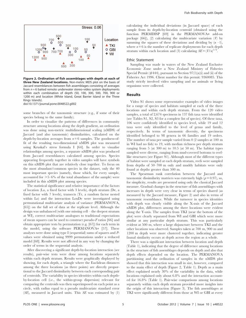
In order to visualize the patterns of differences in community

structure among locations along the depth gradient, an ordination

was done using non-metric multidimensional scaling (nMDS) of

Jaccard (and also taxonomic) dissimilarities, calculated on the

depth-by-location averages from n = 6 samples. The goodness-of-

fit of the resulting two-dimensional nMDS plot was measured

using Kruskal’s stress formula I [64]. In order to visualise

relationships among species, a separate nMDS plot was produced

from Jaccard resemblances calculated among species. Species

appearing frequently together in video samples will have symbols

on this nMDS plot that are relatively close together. To focus on

the most abundant/common species in the dataset, only the 40

most important species (namely, those which, for every sample,

accounted for .5–6% of the total abundance of the sample) were

included in this nMDS plot among species.

The statistical significance and relative importance of the factors

of location (Lo, a fixed factor with 3 levels), depth stratum (De, a

fixed factor with 7 levels), transects (Tr, a random factor nested

within Lo) and the interaction LoxDe were investigated using

permutational multivariate analysis of variance (PERMANOVA,

[65]) on the full set of data at the replicate level. Although the

design was unbalanced (with one missing cell – the deepest stratum

at WI), correct multivariate analogues to traditional expectations

of mean squares can be used to construct pseudo-F ratios [66] and

obtain appropriate tests by permutation (e.g. [67]) for each term in

the model, using the software PERMANOVA+ [57]. These

analyses were done using type I (sequential) sums of squares and P-

values were obtained using 9999 permutations under a reduced

model [68]. Results were not affected in any way by changing the

order of terms in the sequential analysis.

After discovering a significant depth-by-location interaction (see

results), pair-wise tests were done among locations separately

within each depth stratum. Results were graphically displayed by

showing, for each depth, a triangle where the Euclidean distances

among the three locations (as three points) are directly propor-

tional to the Jaccard dissimilarity between each corresponding pair

of centroids. The variability in species identities within each depth-

by-location cell (i.e., the within-group dispersion) relevant for

comparing the centroids was then superimposed on each point as a

circle, with radius equal to a pseudo multivariate standard error

(SE), measured in Jaccard units. This SE was estimated by (1)

calculating the individual deviations (in Jaccard space) of each

sample from its depth-by-location centroid (obtained using the

function PERMDISP [69] in the PERMANOVA+ add-on

package [66]), (2) calculating the multivariate variation (V) by

summing the squares of these deviations and dividing by (n –1),

where n = 6 is the number of replicate deployments for each depth

stratum within each location and (3) calculating SE = (V/n)1/2.

Ethic StatementSampling was made in waters of the New Zealand Exclusive

Economic Zone under a New Zealand Ministry of Fisheries

Special Permit (#444), pursuant to Section 97(1)(a)(i) and (ii) of the

Fisheries Act 1996. Client number for this permit: 9360085. This

study strictly involved video sampling and no animals or living

organisms were collected.

Results

Video S1 shows some representative examples of video images

for a range of species and habitats sampled at each of the three

locations and within each depth stratum. From the 120 video

samples, a total of 2,674 specimens in 137 fish taxa were identified

(see Tables S1, S2, S3 for a complete list of species). Of these taxa,

106 were confidently identified to species level, while 19 and 12

taxa were only identified to the level of genus and family,

respectively. In terms of taxonomic diversity, the specimens

identified belonged to 98 genera in 66 families and 19 orders.

The number of taxa per sample varied from 0 (2 samples at 100 m

in WI had no fish) to 19, with median richness per depth stratum

ranging from 5 (at 300 m) to 10.5 (at 50 m). The habitat types

sampled were diverse, ranging from mud-covered bottoms to reef-

like structures (see Figure S1). Although most of the different types

of habitat were sampled at each depth stratum, reefs were sampled

from depths of 50–700 m only and muddy habitats were only

found at depths greater than 500 m.

The Spearman rank correlation between the Jaccard and

taxonomic dissimilarity matrices was extremely high (r = 0.97), so,

for simplicity, results are presented using only the classical Jaccard

measure. Gradual changes in the structure of fish assemblages with

increases in depth were very clear in terms of species shared (as

measured by the Jaccard measure, Figure 2) and also in terms of

taxonomic resemblance. While the turnover in species identities

with depth was clearly visible along the X-axis of the Jaccard

nMDS plot, differences among the three locations were evident

along the Y-axis. The samples from TKI (near the bottom of the

plot) were clearly separated from WI and GBI which were more

similar at any particular depth stratum. This was particularly

evident at 500 m, where a large disjuncture between TKI and the

other locations was observed. Samples taken at 700 m, 900 m and

1200 m depth were more clustered together, indicating greater

faunal similarity occurs at depth across the region as a whole.

There was a significant interaction between location and depth

(Table 1), indicating that the degree of difference among locations

in the structure of fish assemblages depends on depth and also that

depth effects depended on the location. The PERMANOVA

partitioning and the ordination of samples in the nMDS plot

showed that this interaction was small in size, however, compared

to the main effect of depth (Figure 2, Table 1). Depth as a main

effect explained nearly 30% of the variability in the data, while

locations explained only about 6.8% and the interaction account-

ed for 16.8% (Table 1). Pair-wise comparisons among locations

separately within each depth stratum provided more insights into

the origin of this interaction (Figure 3). The fish assemblages at

TKI were significantly different from those at WI or GBI at every

Figure 2. Ordination of fish assemblages with depth at each ofthree New Zealand locations. Non-metric MDS plot on the basis ofJaccard resemblances between fish assemblages consisting of averagesfrom n = 6 baited remote underwater stereo-video system deploymentswithin each combination of depth (50, 100, 300, 500, 700, 900 or1200 m) and location (White Island, Great Barrier Island or the ThreeKings Islands).doi:10.1371/journal.pone.0048522.g002



depth, with the exception of the 1200 m depth stratum where the

fish assemblages at TKI did not differ significantly from those at

GBI. In shallow water (50 m and 100 m), the fish assemblages

were significantly different between WI and GBI, but there were

no significant differences between these two locations for any of

the deeper strata (300 m and deeper).

Furthermore, at each location, most fish assemblages were

significantly different between all pairs of depth strata (Table 2).

However, there were no significant differences detected between

50 and 100 m depth strata at any of the locations. Similarly,

comparisons between adjacent depth strata at intermediate depths

(100 vs 300 m, 300 vs 500 m, and 500 vs 700 m) were not

statistically significant at any location, indicating a gradual change

in faunal composition as seen in the nMDS plot (Figure 2). This

was also true at deeper depths for WI and GBI, but at TKI there

was apparently more stratification, as significant differences were

found between adjacent pairs of assemblages for the deep strata

(i.e., 700 vs 900 m and 900 vs 1200 m, Table 2).

Patterns in univariate diversity measures along the depth

gradient were examined separately at each of the three locations

(Figure 4). Average values of species richness ranged from 4.3 to

14.2, Simpson’s evenness from 0.53 to 0.98, average taxonomic

distinctness (g+) from 74 to 93 and variation in taxonomic

distinctness (L+) from 62 to 482. Species richness showed a clear

peak in shallow depth strata with particularly higher average

richness observed at the northern location (TKI), followed by a

decrease beyond 100 m and a stable common trend of an average

number of ca. 7 species recorded per video deployment from 700

to 1200 m (Figure 4a). The decrease in species richness from 100

to 300 m was particularly sharp for TKI. Minima in average

species richness occurred deeper at the northern sites, with TKI,

GBI and WI having their minima at 500, 300 and 100 m,

respectively. It is also clear that in shallower strata, the variability

among samples in species richness was greater than in deeper

strata. From 700 m onwards, variability in species richness for all

locations decreased with depth. Evenness was also more variable

at shallow depths, but with a trend of increasing evenness to a

depth of about 700 m, followed by a decrease in mean evenness to

1200 m (Figure 4b). Similarly, average taxonomic distinctness g+

was also unimodal, but with a peak at 300 m for all locations

(Figure 4c). The variability of g+ was especially high among

samples at the 100 m depth stratum and low at deeper depths.

Finally, the variation in taxonomic distinctness L+ first decreased

sharply from 50 to 300 m, then increased beyond 500 m depth,

indicating that the taxonomic tree of deeper samples had more

variable path-lengths than did shallower samples (Figure 4d).

Species from deep samples belonged to more distant taxonomic

groups that those from shallow samples.

Pooling the n = 6 samples taken at a given depth and location,

species richness ranged from 10 to 26 (Figure 5). At each location,

lower total species richness was displayed at some intermediate

depth, with relatively high species richness in the shallow (50 m)

and deeper strata (500–700 m). This low total species richness was

observed at 100, 300 and 500 m for WI, GBI and TKI,

respectively. A similar trend was observed at the family level.

Compared to the species level, the richness at family level tended

to more sharply decrease at the deepest depths, indicating clusters

of species within fewer families.

Associations between species are shown in Figure 6, and the

occurrences in the different depth strata of the 20 most abundant

taxa at each location are shown graphically in Figure 7. Typically,

a set of species associated with one another (Figure 6) occurred

primarily within certain depth strata (Figures 6 and 7). A depth

gradient is also evident in these inter-specific associations

(Figure 6), as illustrated by examining the average depth of

occurrence for each species. In shallow depth strata, the most

abundant species were similar across all locations and the fish

fauna was characterized by greater frequencies (and co-occur-

rence) of Pseudocaranx georgianus (Cuvier 1833), Pagrus auratus (Forster

1801), Centroberyx affinis (Gunther 1859), Caprodon longimanus

(Gunther 1859) and Seriola lalandi Valenciennes 1833 (Figure 7).

At TKI, Caesioperca lepidoptera (Forster 1801), Suezichthys aylingi

Russell 1985, Pseudolabrus miles (Schneider & Forster 1801) and

Nemadactylus n.sp were also closely associated at typically 70–120 m

depth. TKI had the greatest range in fish abundances, as

measured using sum of the values of MaxN pooled across the

n = 6 samples (i.e., N = 1–367), with three species showing greatest

total abundances: schooling Caprodon longimanus (N = 367) and

Caesioperca lepidoptera (N = 197) and Suezichthys aylingi (N = 192).

Nemadactylus macropterus (Forster 1801), Galeorhinus galeus (Linnaeus

1758), Cephaloscyllium isabellum (Bonnaterre 1788), Parapercis gilliesi

(Hutton 1879) and Squalus griffini Phillipps 1931 were typical of the

150–300 m depth range. Polyprion americanus (Bloch & Schneider

1801), an undescribed species of hagfish Eptatretus sp.2 and

Cirrhigaleus australis White, Last & Stevens 2007 were closely

associated at average depths of 390 to 540 m, especially at TKI.

Macruronus novaezelandiae (Hector 1871) and Genypterus blacodes

(Forster 1801) were observed in samples having an average depth

of just over 600 m. In the depth band 650 to 830 m, Deania calcea

(Lowe 1839), Bassanago bulbiceps Whitley 1948, Mora moro (Risso

1810) and Myctophidae spp commonly co-occurred. The deepest

station had three synaphobranchids (Simenchelys parasitica Gill 1879,

Synaphobranchus affinis Gunther 1877 and Diastobranchus capensis

Barnard 1923) and two sharks (Centroscymnus owstoni Garman 1906

and Etmopterus baxteri Garrick 1957) as characteristic species.

Generally, the most abundant species occurred within relatively

narrow depth bands (Figure 7). A few species, like the hagfishes

Neomyxine sp.1 and Eptatretus cf.cirrhatus (Forster 1801) or the dogfish

Squalus griffini Phillipps 1931 occurred across a depth range of

more than 700 m.

Some species were common at all three locations: Seriola lalandi

(N = 34, 27, 15, for TKI, GBI and WIs, respectively), Mora moro

(N = 20, 17, 12), Helicolenus sp. (N = 14, 14, 19), Deania calcea (N = 3,

Table 1. PERMANOVA results for the analysis of fishassemblages on the basis of the Jaccard resemblancemeasure in response to location, depth stratum and transect.

Source df MS Pseudo-F PSqrt(Componentof variation) %

Lo 2 15,898 6.38 0.0001 18.505 6.8%

De 6 27,086 11.57 0.0001 38.486 29.4%

Tr (Lo) 15 2,491 1.06 0.1413 4.780 0.5%

Lo6De 11 7,300 3.12 0.0001 29.079 16.8%

Res 83 2,341 48.388 46.5%

Total 117

Location (Lo, fixed, 3 levels), depth stratum (De, fixed, 7 levels) and transect (Tr,random, nested within Lo, 6 replicates). Similar results were obtained using thetaxonomic resemblance measure (C+). Partitioning was done using Type I(sequential) sums of squares and P-values were obtained for each term using9999 permutations under the reduced model. The estimated sizes of effects foreach term in the model are shown in Jaccard units as the square root of thecomponents of variation, and variation attributable to each individual term isalso expressed as a percentage of the total (%). Note that 2 of the original 120samples were omitted prior to analysis, as there were no fish recorded in thosedeployments.doi:10.1371/journal.pone.0048522.t001



8, 9), Gadomus aoteanus (N = 3, 4, 2), Genypterus blacodes (N = 3, 3, 3).

However, most species were common or abundant at just one

location and absent or present in low numbers elsewhere. For

example, at TKI, prevalent taxa included the hagfish Eptaptretus

sp.2 (N = 33, 0, 0), Parika scaber (N = 30, 1, 1), Nemadactylus n.sp.

(N = 29, 1, 1), Polyprion americanus (N = 18, 0, 1) and Proscymnodon

plunketi (N = 15, 1, 0). Conversely, some species that were absent or

had low abundance at TKI were more numerous at the other

locations: e.g., Eptaptretus cf.cirrhatus (N = 0, 53, 57), Pseudocaranx

Figure 3. Pair-wise comparisons of fish assemblages amonglocations at each depth. Graphical representation of PERMANOVApair-wise tests comparing fish assemblages among locations separatelyfor each depth stratum on the basis of the Jaccard resemblancemeasure. Triangle side lengths are proportional to the Jaccarddissimilarities between location centroids. Circle radii are proportionalto a pseudo multivariate standard error around the group centroid foreach location within each depth. Due to the large number ofcomparisons, a conservative significance level of a= 0.01 was used.Significant differences (p,0.01) are marked by an asterisk (*).Partitioning was done using Type I (sequential) sums of squares andP-values were obtained for each term using 9999 permutations underthe reduced model. Similar results were obtained using the taxonomicresemblance measure G+.doi:10.1371/journal.pone.0048522.g003

Table 2. PERMANOVA pair-wise comparisons of fishassemblages at different depths done separately at eachlocation on the basis of the Jaccard resemblance measure.

Pair of depth stratabeing compared (m) P value

TKI GBI WI

50 vs100 0.047 0.103 0.106

50 vs 300 0.003 0.002 0.002

50 vs 500 0.002 0.003 0.002

50 vs 700 0.002 0.003 0.008

50 vs 900 0.003 0.004 0.002

50 vs 1200 0.002 0.003 –

100 vs 300 0.012 0.019 0.036

100 vs 500 0.003 0.008 0.020

100 vs 700 0.004 0.005 0.043

100 vs 900 0.003 0.004 0.013

100 vs 1200 0.002 0.004 –

300 vs 500 0.135 0.016 0.014

300 vs 700 0.101 0.005 0.017

300 vs 900 0.003 0.002 0.003

300 vs 1200 0.002 0.002 –

500 vs 700 0.096 0.020 0.048

500 vs 900 0.002 0.004 0.002

500 vs 1200 0.003 0.002 –

700 vs 900 0.002 0.043 0.033

700 vs 1200 0.002 0.003 –

900 vs 1200 0.007 0.022 –

Partitioning was done using Type I (sequential) sums of squares and P-valueswere obtained for each term using 9999 permutations under the reducedmodel. Similar results were obtained using taxonomic resemblances C+. Due tothe large number of comparisons, a conservative level of a= 0.01 was chosen.Significant p-values (,0.01) are shown in bold.doi:10.1371/journal.pone.0048522.t002



georgeanus (N = 7, 14, 29), Bassanago bulbiceps (N = 3, 16, 10),

Cephaloscylium isabellum (N = 3, 17, 4) and Rexea solandri (N = 1, 8,

8). Nemadactylus macropterus was common at TKI, but nearly twice

as abundant at GBI and four times as abundant at WI.

Fishes endemic to New Zealand occurred at all three locations

(TKI, GBI, WI) and within most depth strata sampled, ranging

from a minimum of 48 m to a maximum of 1275 m depth (Table 3

and Tables S1, S2, S3). The percentage of endemic fishes was

highest at TKI (22.1%) and GBI (21.0%), and lowest off WI

(12.0%). Interestingly, the percentage of endemic fishes was

highest at shallow depths (50 m or 100 m) and also at very deep

depths (900 m or 1200 m), where they made up.20% of the fish

taxa that were recorded (Table 3). The occurrence of endemics

was lowest, however, at intermediate depths (from 300–800 m).

In terms of geographical distributions, there was only one

species recorded from the video footage that could be classified as

a southern species – the girdled wrasse (Notolabrus cinctus), although

it has been recorded at TKI before [51]. It was found at just one

location and depth stratum (TKI, 109 m). The percentage of fishes

with a particular biogeographical distribution varied with depth.

Widespread species were least common at middle depths (300–

700 m, 17.1%) and most common at shallow depths (50–300 m,

31.6%) and deeper depths (700–1200 m, 51.2%). Northern species

were most common in shallow water (50–300 m, 62.7%),

progressively decreasing in numbers with depth (700–1200 m,

10.5%).

Figure 4. Relationships between fish biodiversity indices and depth. Plots showing the mean 61 SD (n = 6) for each of (a) species richness,(b) Simpson’s evenness, (c) average taxonomic distinctness, D+ and (d) variation in taxonomic distinctness, L+ for fish assemblages versus depth ateach of three locations.doi:10.1371/journal.pone.0048522.g004



Figure 5. Family and species richness of fishes identified from video samples by depth and location. Each circle pools the informationobtained from n = 6 two-hour video deployments and its diameter is proportional in size to the richness value at one location. Overall totals fordepths and locations are given in the marginal columns and rows, respectively, with the grand total given in the bottom right-hand corner.doi:10.1371/journal.pone.0048522.g005



Discussion

There was a strong gradient of change in the diversity and

community structure of fishes observed using stereo-BRUV

deployments along the New Zealand continental shelf and slope.

Clear turnover in the identities of species was observed with

increasing depth, and this was mirrored by turnover in taxonomic

resemblances. Although video deployments at different depths

were separated spatially by just hundreds of metres, depth effects

greatly exceeded location effects, which spanned hundreds of

kilometres, and regional similarities in the fish fauna became

apparent at the deeper depths, where differences among locations

were no longer statistically significant. Traditionally, fish assem-

blages have been divided into shelf (50 to ,300 m), upper slope

(300 to ,900 m), middle slope and lower slope (2000 to ,4000 m)

assemblages [70]. This pattern has been confirmed at different

locations [27,71,72,73]. Our observations suggest a more gradual

continuum of change in fish assemblages with depth. Although an

initial zone does appear to exist up to ,100 m, comparisons of

samples taken from deeper adjacent depth strata (i.e., 100 vs

300 m, 300 vs 500 m, and 500 vs 700 m) were not strongly

dissimilar, indicating a progressive turnover of species rather than

a distinct zonation of species with restricted depth ranges. At

700 m depth, another pattern emerged. The fish fauna of deeper

strata (700 to 1200 m) displayed faster turnover, however,

especially at the Three Kings Islands, the most northern location.

This depth range (700–1200 m) may represent a zone of transition

between the upper and lower-slope fauna. In his extensive data

analysis of New Zealand demersal fish fauna, Francis [73]

identified inshore (0–60 m), shelf (50–300 m), upper slope (400–

740 m) and mid-slope (720–1320 m) assemblages. Similar bound-

aries and affinities in the composition of mid-slope fauna have

been documented in south-eastern and western Australia [74,75].

Comparing the species lists from our study and Koslow [74], we

find that more than 50% of the New Zealand species are found on

both sides of the Tasman Basin for the depth range from 700 to

1200 m. Antarctic Intermediate Waters of low salinity extend to

New Zealand within this particular depth range, and might be one

of the drivers of such a distinct zone [76], coinciding with a

distribution of relatively similar fish fauna across the South Pacific

and Atlantic [74,75,77,78].

Both individual sample and location-scale species richness were

relatively high in the shallower strata (50 m) and then decreased to

reach a minimum at a depth which depended on the location.

Minimal species richness at intermediate depths (e.g., at 500 m on

the U.S. Pacific coast, [26]) has been linked with an oxygen

Figure 6. Ordination of fish species associations, with average depth as bubbles. Non-metric MDS plot of the Jaccard resemblancesamong the 40 most important fish species in the dataset, based on their frequencies of occurrences. Species which co-occur together often will havehigh Jaccard similarity, and will be placed by the nMDS algorithm relatively close together on the plot. The 40 most important species are thosewhich, for every sample, account for .5–6% of a sample’s total abundance. The relative average depth of the samples at which each species occurredis shown using scaled bubbles. The average depth (in metres) at which each species was recorded is also shown numerically in the centre of eachbubble.doi:10.1371/journal.pone.0048522.g006



minimum zone [79]. In our case, however, the shallow depth at

WI where minimal richness occurred (100 m) is more likely to

have been caused by toxic volcanic activity at that particular

location. In southern New Zealand waters, Some possible

explanations for an increase in the depth at which minimum

richness occurs at northerly locations include: (i) greater stability in

seasonal climate conditions, (ii) greater substratum heterogeneity

in deeper waters at TKI, or (iii) two different oceans meeting at

TKI to generate oceanographic confluence, mixing and upwelling,

thereby increasing overall richness and also extending the depth at

which greater richness occurs.

Overall, evenness tended to increase with depth, in agreement

with our prediction that fish species in deeper habitats would be

more uniformly abundant due to a reduced input of energy. A

drop in evenness was observed for the 1200 m strata. These deep

samples were dominated by two species of synaphobranchid eels

(Diastobranchus capensis and Synaphobranchus affinis) which appeared in

relatively high numbers compared to other species. At White

Island, low average evenness occurred at 100 m, explained by

having two samples with no species and the other samples

dominated by either Centroberyx affinis or Nemadactylus macropterus.

These species form schools, especially in deeper waters [51]. On

the U.S. Pacific coast, evenness in groundfish assemblages was

observed to be high in shallow water (200–500 m), lower at 600–

900 m and then higher again at 1000–1200 m [26]. It is difficult

to discern spatial or environmental patterns of evenness from trawl

data such as these, however, due to the selectivity of trawling gear

for particular types of species [26].

Average taxonomic distinctness (highest at 300 m) showed an

opposite trend to the variation in taxonomic distinctness (lowest at

300 m). The low value of average taxonomic distinctness at

shallow depths can be explained by the predominance of species

which are closely associated in the taxonomic tree. Between 300

and 700 m, the proportion of Chondrichthyes relative to

Osteichthyes was larger than at either shallower or deeper depths,

leading to higher AvTD values. Both ends of the depth spectrum

measured here showed high variation in taxonomic distinctness,

indicating taxonomically distinct clusters of highly related species

occur at these two extremes (i.e. 50 m and 1200 m) [42]. It

appears that some lineages have specialized for the deep-sea

environment [80]; members of the Macrouridae and Alepocepha-

lidae have been noted to dominate in deep-sea environments [16],

along with Synaphobranchidae, Moridae and Ophiididae [81].

In addition to rapid faunal turnover beyond 700 m, we

observed increasing similarities among the fauna of the deeper

samples across locations. A decrease in fish diversity with depth

may reflect a decrease in habitat heterogeneity [82]. Turnover

could also be driven at large scales by organic carbon flux to the

seafloor [83], as would be predicted by a general positive species-

energy relationship [8]. Rex and Etter [83] suggested that limited

food supply at depth for larger animals would also limit population

size, which in turn would negatively affect diversity [8]. The extent

to which there are increased affinities in fish assemblages with

increasing depth, despite large separations among locations, as

found here, may or may not be maintained at larger spatial scales.

For example, deep-sea demersal fish assemblages of seamounts

have strong affinities at the regional scale (100 to a few 1000’s km),

but not at larger oceanic scales, where other factors, probably

historical, came into play [77].

In this study, we identified 137 taxa (mostly to species) from 120

stereo-BRUV deployments. The number of taxa observed here by

stereo-BRUVs compares favourably with the diversity measured in

other studies using trawls, although we used a less intensive

sampling scheme. For example, in New Zealand’s subantarctic

region, Jacob [84] sampled 102 fish taxa from 363 bottom trawls

at depths ranging from 80 to 787 m.

Our study recorded a total of 117 species of fishes with

widespread distributions and 67 species of northern fishes from the

Figure 7. Occurrence of the most abundant fish taxa withdepth. The frequencies of occurrence (out of n = 6 samples) for each ofthe 20 most abundant taxa at each depth and across each of the threelocations are presented. For each location, the species are ordered fromshallow to deep, with the most common species at a particular depthbeing cited first.doi:10.1371/journal.pone.0048522.g007



three areas sampled. This is the first time that widespread and

northern fishes have been recorded occurring in such high

numbers and extending to such great depths (1275 m) off New

Zealand. However, fishes with northern distributions progressively

decreased in their proportional representation with depth whereas

those with widespread distributions increased. One explanation for

this could be the tolerance of species to water temperature. It is

perhaps surprising, however, that northern species occur at all past

300 m depth, where temperatures are usually below 10uC. Here,

we documented northern species occurring in all depth strata

sampled down to 1275 m, where bottom temperatures of 4–6uCare the norm. Surface temperatures this low would be found well

south of subantarctic New Zealand in the Southern Ocean. Thus,

the dynamics of individual species’ distributions with depth is

clearly more complex than a simple physiological response to

temperature that might be inferred from known geographic

ranges.

In addition to being non-destructive, a valuable further

advantage to using video systems is the relatively high level of

consistency of the sample across a variety of habitats. The

efficiency of trawls varies over different habitats, so different types

of trawl might be required in order to evaluate overall fish diversity

[42,85]. Baited video systems can be deployed over virtually any

kind of habitat, including difficult terrain, such as rough substrata

encountered at seamounts [86]. We have used video units with a

high success rate over shallow and deep (1200 m) reef systems

where trawls would have failed. One might expect that baited

cameras will primarily sample effectively only those fish species

attracted to bait, or to the lights or activities of other organisms

around the bait. Previous studies in shallow water indicate that

baited systems can be used to sample a range of trophic groups

successfully, including herbivores and omnivores, as well as

predatory and scavenging fish species [20]. Nevertheless, the

responses of fishes to bait can vary with changes in oceanographic

conditions, such as current speed and temperature. Thus deep

deployments may attract a different fraction of the ichthyofauna

over a similar time frame – a topic worthy of further investigation.

Beyond 1500 m, studies have shown that the trophic groups

attracted to bait are not only scavengers, but also opportunistic

scavengers that are otherwise predators [87,88]. In this study, both

predators and scavengers were observed up to 1200 m, although

the primary feeding behaviour of many if not most of the species

we recorded at such depths is still largely unknown. Future studies

would benefit from comparisons of baited video with other

recently developed un-baited video techniques for studying

biodiversity and its relationship with habitat characteristics(e.g.

[89]).

This study has provided the first characterization of diversity

patterns for bait-attracted fish species on continental slopes in New

Zealand. This essential observational knowledge of the fine-scale

distribution patterns of individual fish species with depth is an

imperative primary step towards development of explanatory and

predictive ecological models, as well as being fundamental for the

implementation of efficient management and conservation strat-

egies for fishery resources.

Supporting Information

Figure S1 Number of video samples taken over differ-ent types of habitat, as indicated, within each depthstratum.

(PDF)

Table S1 Taxa identified from video deployments atthree locations in New Zealand waters (ordered phylo-genetically).

(PDF)

Table S2 Taxa identified from video deployments atthree locations in New Zealand waters (ordered alpha-betically).

(PDF)

Table S3 Taxa identified from video deployments atthree locations in New Zealand waters, arranged bytheir occurrence within each of seven depth strata (50,100, 300, 500, 700, 900 and 1200 m).

(PDF)

Video S1 Selection of video footage showing typicalexamples of observed fish species attracted to baitedremote underwater video systems in New Zealandwaters. Representative footage from three locations (Three

Kings Islands, Great Barrier Island and White Island) and seven

depth strata are presented (50, 100, 300, 500, 700, 900 and

1200 m).

(MP4)

Table 3. Occurrence by depth strata of fish species having different biogeographical distributions{ in New Zealand waters.

Depth (m) Distribution Total

Northern Southern Widespread

All Endemic All Endemic All Endemic All Endemic

50–99 22 (33%) 4 (22%) 0 0 20 (17%) 8 (36%) 42 (23%) 12 (29%)

100–299 20 (30%) 3 (17%) 1 1 17 (15%) 4 (18%) 38 (21%) 8 (20%)

300–499 10 (15%) 5 (28%) 0 0 8 (7%) 1 (5%) 18 (10%) 6 (15%)

500–699 8 (12%) 1 (6%) 0 0 12 (10%) 2 (9%) 20 (11%) 3 (7%)

700–899 5 (7%) 3 (17%) 0 0 21 (18%) 0 (0%) 26 (14%) 3 (7%)

900–1200 2 (3%) 2 (11%) 0 0 39 (33%) 7 (32%) 41 (22%) 9 (22%)

Total 67 18 1 1 117 22 185 41

{Definitions of northern, southern or widespread biogeographical distributions are given in the text. Results are also presented for species known to be endemic to NewZealand waters.doi:10.1371/journal.pone.0048522.t003



Acknowledgments

The MV Tranquil Image crew N. Furley, G. Gibbs and S. Kelly helped to

organize all of the fieldwork using baited underwater video units. R.

Crech’riou, A. Smith, C. Bedford, O. Hannaford and K. Rodgers

contributed to the sampling effort. P. McMillan (Macrouridae), P. Last and

C. Duffy with (sharks), and D. Smith (Synaphobranchidae) helped with

species identifications on videos.

Author Contributions

Conceived and designed the experiments: VZ MJA CR EH. Performed the

experiments: VZ CS. Analyzed the data: VZ MJA CR. Contributed

reagents/materials/analysis tools: VZ MJA CR EH AS CS. Wrote the

paper: VZ MJA CR EH AS CS.

References

1. Carney RS (2005) Zonation of deep biota on continental margins. Oceanog-

raphy and Marine Biology: An Annual Review 43: 211–278.

2. Duffy JE (2009) Why biodiversity is important to the functioning of real-world

ecosystems. Frontiers in Ecology and the Environment 7: 437–444.

3. Worm B, Barbier EB, Beaumont N, Duffy JE, Folke C, et al. (2006) Impacts of

biodiversity loss on ocean ecosystem services. Science 314: 787–790.

4. Balvanera P, Pfisterer AB, Buchmann N, He JS, Nakashizuka T, et al. (2006)

Quantifying the evidence for biodiversity effects on ecosystem functioning and

services. Ecology Letters 9: 1146–1156.

5. Cardinale BJ, Srivastava DS, Duffy JE, Wright JP, Downing AL, et al. (2006)

Effects of biodiversity on the functioning of trophic groups and ecosystems.

Nature 443: 989–992.

6. Hooper DU, Chapin FS, Ewel JJ, Hector A, Inchausti P, et al. (2005) Effects of

biodiversity on ecosystem functioning: A consensus of current knowledge.

Ecological Monographs 75: 3–35.

7. Willig MR, Kaufman DM, Stevens RD (2003) Latitudinal gradients of

biodiversity: Pattern, process, scale, and synthesis. Annual Review of Ecology,

Evolution and Systematics 34: 273–309.

8. Evans KL, Warren PH, Gaston KJ (2005) Species-energy relationships at the

macroecological scale: a review of the mechanisms. Biological Reviews of the

Cambridge Philosophical Society 80: 1–25.

9. Helfman GS, Collette BB, Facey DE, Bowen BW (2009) The Diversity of Fishes

- Biology, Evolution and Ecology. Oxford: Wiley-Blackwell. 720 p.

10. Holmlund CM, Hammer M (1999) Ecosystem services generated by fish

populations. Ecological Economics 29: 253–268.

11. Myers RA, Baum JK, Shepherd TD, Powers SP, Peterson CH (2007) Cascading

effects of the loss of apex predatory sharks from a coastal ocean. Science 315:

1846–1850.

12. Blanco M, Sotelo CG, Chapela MJ, Perez-Martın RI (2007) Towards

sustainable and efficient use of fishery resources: present and future trends.

Trends in Food Science & Technology 18: 29–36.

13. Anderson TJ, Yoklavich MM (2007) Multiscale habitat associations of deepwater

demersal fishes off central California. Fishery Bulletin 105: 168–179.

14. Ross SW, Quattrini AM (2007) The fish fauna associated with deep coral banks

off the southeastern United States. Deep-Sea Research Part I: Oceanographic

Research Papers 54: 975–1007.

15. Trenkel VM, Francis RICC, Lorance P, Mahevas S, Rochet MJ, et al. (2004)

Availability of deep-water fish to trawling and visual observation from a remotely

operated vehicle (ROV). Marine Ecology Progress Series 284: 293–303.

16. Merrett NR, Gordon JDM, Stehmann M, Haedrich RL (1991) Deep demersal

fish assemblage structure in the Porcupine Seabight (eastern North-Atlantic):

Slope sampling by 3 different trawls compared. Journal of the Marine Biological

Association of the UK 71: 329–358.

17. Trenkel VM, Lorance P, Mahevas S (2004) Do visual transects provide true

population density estimates for deepwater fish? ICES Journal of Marine Science

61: 1050–1056.

18. Stoner AW, Ryer CH, Parker SJ, Auster PJ, Wakefield WW (2008) Evaluating

the role of fish behavior in surveys conducted with underwater vehicles.

Canadian Journal of Fisheries and Aquatic Sciences 65: 1230–1243.

19. Gray JS (2001) Marine diversity: the paradigms in patterns of species richness

examined. Scientia Marina 65: 41–56.

20. Harvey ES, Cappo M, Butler JJ, Hall N, Kendrick GA (2007) Bait attraction

affects the performance of remote underwater video stations in assessment of

demersal fish community structure. Marine Ecology Progress Series 350: 245–

254.

21. Rex MA (1983) Geographical patterns of species diversity in the deep-sea

benthos. In: Rowe GT, editor. The Sea Vol 8: Deep-Sea Biology. New York:

Wiley Interscience. pp. 453–472.

22. Gray JS (2000) The measurement of marine species diversity, with an

application to the benthic fauna of the Norwegian continental shelf. Journal of

Experimental Marine Biology and Ecology 250: 23–49.

23. Levin LA, Etter RJ, Rex MA, Gooday AJ, Smith CR, et al. (2001)

Environmental influences on regional deep-sea species diversity. Annual Review

of Ecology and Systematics 32: 51–93.

24. Gage JD, Tyler PA (1991) Deep-sea biology: a natural history of organisms at

the deep-sea floor. Cambridge: Cambridge University Press. 509 p.

25. Wei CL, Rowe GT, Hubbard GF, Scheltema AH, Wilson GDF, et al. (2010)

Bathymetric zonation of deep-sea macrofauna in relation to export of surface

phytoplankton production. Marine Ecology-Progress Series 399: 1–14.

26. Tolimieri N (2007) Patterns in species richness, species density, and evenness in

groundfish assemblages on the continental slope of the US Pacific coast.

Environmental Biology of Fishes 78: 241–256.

27. Moranta J, Stefanescu C, Massuti E, Morales-Nin B, Lloris D (1998) Fish

community structure and depth-related trends on the continental slope of the

Balearic Islands (Algerian basin, western Mediterranean). Marine Ecology

Progress Series 171: 247–259.

28. Lorance P, Souissi S, Uiblein F (2002) Point, alpha and beta diversity of

carnivorous fish along a depth gradient. Aquatic Living Resources 15: 263–271.

29. Smith KF, Brown JH (2002) Patterns of diversity, depth range and body size

among pelagic fishes along a gradient of depth. Global Ecology and

Biogeography 11: 313–322.

30. Leathwick JR, Elith J, Francis MP, Hastie T, Taylor P (2006) Variation in

demersal fish species richness in the oceans surrounding New Zealand: an

analysis using boosted regression trees. Marine Ecology Progress Series 321:

267–281.

31. Sousa P, Azevedo M, Gomes MC (2006) Species-richness patterns in space,

depth, and time (1989–1999) of the Portuguese fauna sampled by bottom trawl.

Aquatic Living Resources 19: 93–103.

32. Magnussen E (2002) Demersal fish assemblages of Faroe Bank: species

composition, distribution, biomass spectrum and diversity. Marine Ecology

Progress Series 238: 211–225.

33. Magurran AE (2004) Measuring biological diversity. Oxford: Blackwell

Publishing. 256 p.

34. Hillebrand H, Bennett DM, Cadotte MW (2008) Consequences of dominance: a

review of evenness effects on local and regional ecosystem processes. Ecology 89:

1510–1520.

35. Jetz W, Rahbek C, Colwell RK (2004) The coincidence of rarity and richness

and the potential signature of history in centres of endemism. Ecology Letters 7:

1180–1191.

36. Rahbek C, Gotelli NJ, Colwell RK, Entsminger GL, Rangel T, et al. (2007)

Predicting continental-scale patterns of bird species richness with spatially

explicit models. Proceedings of the Royal Society B-Biological Sciences 274:

165–174.

37. Laliberte E, Legendre P (2010) A distance-based framework for measuring

functional diversity from multiple traits. Ecology 91: 299–305.

38. Clarke KR, Warwick RM (1998) A taxonomic distinctness index and its

statistical properties. Journal of Applied Ecology 35: 523–531.

39. Clarke KR, Warwick RM (2001) A further biodiversity index applicable to

species lists: variation in taxonomic distinctness. Marine Ecology Progress Series

216: 265–278.

40. Tolimieri N, Anderson MJ (2010) Taxonomic distinctness of demersal fishes of

the California current: moving beyond simple measures of diversity for marine

ecosystem-based management. Plos One 5.

41. Merigot B, Bertrand JA, Gaertner JC, Durbec JP, Mazouni N, et al. (2007) The

multi-component structuration of the species diversity of groundfish assemblages

of the east coast of Corsica (Mediterranean Sea): Variation according to the

bathymetric strata. Fisheries Research 88: 120–132.

42. Zintzen V, Anderson MJ, Roberts CD, Diebel CE (2011) Increasing variation in

taxonomic distinctness reveals clusters of specialists in the deep sea. Ecography

34: 306–317.

43. Cappo M, Harvey ES, Shortis M. Counting and measuring fish with baited

video techniques - an overview. In: Furlani D, Beumer JP, editors; 2006; Hobart,

Australia, August 2007. Australian Society for Fish Biology. pp. 101–114.

44. Harvey ES, Shortis M, Stadler M, Cappo M (2002) A comparison of the

accuracy and precision of measurements from single and stereo-video systems.

Marine Technology Society Journal 36: 38–49.

45. Douglas RH, Partridge JC, Marshall NJ (1998) The eyes of deep-sea fish I: lens

pigmentation, tapeta and visual pigments. Progress in Retinal and Eye Research

17: 597–636.

46. Harvey ES, Goetze J, McLaren B, Langlois T, Shortis MR (2010) Influence of

range, angle of view, image resolution and image compression on underwater

stereo-video measurements: high-definition and broadcast-resolution video

cameras compared. Marine Technology Society Journal 44: 75–85.

47. Harvey ES, Shortis MR (1996) A system for stereo-video measurement of sub-

tidal organisms. Marine Technology Society Journal 29: 10–22.

48. Priede IG, Bagley PM, Smith A, Creasey S, Merrett NR (1994) Scavenging deep

demersal fishes of the Porcupine Seabight, north-east Atlantic: observations by

baited camera, trap and trawl. Journal of the Marine Biological Association of

the UK 74: 481–498.



49. Cappo M, Speare P, De’ath G (2004) Comparison of baited remote underwater

video stations (BRUVS) and prawn (shrimp) trawls for assessments of fishbiodiversity in inter-reefal areas of the Great Barrier Reef Marine Park. Journal

of Experimental Marine Biology and Ecology 302: 123–152.

50. Cappo MC, Harvey ES, Malcolm HA, Speare PJ (2003) Potential of video

techniques to design and monitor diversity, abundance and size of fish in studiesof Marine Protected Areas. World Congress on Aquatic Protected Areas

proceedings Aquatic Protected Areas - what works best and how do we know?

Cairns, Australia: Australian Society of Fish Biology. pp. 455–464.

51. Francis MP (2001) Coastal fishes of New Zealand. Auckland: Reed Books.

52. Last PR, Stevens JD (2009) Shark and Rays of Australia. Collingwood, Australia:

CSIRO Publishing. 644 p.

53. Paulin CD, Roberts CD (1992) The Rockpool fishes of New Zealand, Te ika

aaria o Aotearoa. Wellington: Museum of New Zealand Te Papa Tongarewa.177 p.

54. Paulin CD, Roberts CD (1993) Biogeography of New Zealand rockpool fishes.

In: Battershill CN, Schiel DR, Jones GP, Creese RG, MacDairmid AB, editors.

Proceedings of the Second International Temperate Reef Symposium.University of Auckland, New Zealand: NIWAR Marine, Wellington. pp. 191–

199.

55. Paulin CD, Stewart AL (1985) A list of New Zealand teleost fishes held in the

National Museum of New Zealand. National Museum of New Zealand,Miscellaneous Series 12: 1–63.

56. Clarke KR, Gorley RN (2006) PRIMER v6: User manual/Tutorial. Plymouth,UK: PRIMER-E Ltd. 190 p.

57. Anderson MJ, Gorley RN, Clarke KR (2008) PERMANOVA+ for PRIMER:

Guide to Software and Statistical Methods. Plymouth: PRIMER-E Ltd. 214 p.

58. Simpson EH (1949) Measurement of diversity. Nature 163: 688.

59. Smith B, Wilson JB (1996) A consumer’s guide to evenness measures. Oikos 76:70–82.

60. Nelson JS (2006) Fishes of the world. Hoboken, New Jersey: Wiley & Sons. 601 p.

61. Eschmeyer WN (2008) Catalog of Fishes. Available: http://www.calacademy.org/research/ichthyology/catalog/fishcatsearch.html. Accessed 2008 August

29.

62. Jaccard P (1900) Contribution au probleme de l’immigration post-glaciaire de la

flore alpine. Bulletin de la Societe Vaudoise des Sciences naturelles 36: 87–130.

63. Clarke KR, Somerfield PJ, Chapman MG (2006) On resemblance measures for

ecological studies, including taxonomic dissimilarities and a zero-adjusted Bray-Curtis coefficient for denuded assemblages. Journal of Experimental Marine

Biology and Ecology 330: 55–80.

64. Kruskal JB, Wish M (1978) Multidimensional scaling. Beverly Hills: Sage

Publications. 86 p.

65. Anderson MJ (2001) A new method for non-parametric multivariate analysis ofvariance. Austral Ecology 26: 32–46.

66. McArdle BH, Anderson MJ (2001) Fitting multivariate models to communitydata: a comment on distance-based redundancy analysis. Ecology 82: 290–297.

67. Anderson MJ, ter Braak CJF (2003) Permutation tests for multi-factorial analysisof variance. Journal of Statistical Computation and Simulation 73: 85–113.

68. Freedman D, Lane D (1983) A nonstochastic interpretation of reported

significance levels. Journal of Business and Economic Statistics 1: 292–298.

69. Anderson MJ (2006) Distance-based tests for homogeneity of multivariate

dispersions. Biometrics 62: 245–253.

70. Haedrich RL, Merrett NR (1988) Summary atlas of deep-living demersal fishes

in the North-Atlantic basin. Journal of Natural History 22: 1325–1362.

71. Kallianiotis A, Sophronidis K, Vidoris P, Tselepides A (2000) Demersal fish and

megafaunal assemblages on the Cretan continental shelf and slope (NEMediterranean): seasonal variation in species density, biomass and diversity.

Progress in Oceanography 46: 429–455.

72. Powell SM, Haedrich RL, McEachran JD (2003) The deep-sea demersal fishfauna of the Northern Gulf of Mexico. Journal of Northwest Atlantic Fishery

Science 31: 19–33.73. Francis MP, Hurst MJ, MacArdle BH, Bagley N, Anderson OF (2002) New

Zealand demersal fish assemblages. Environmental Biology of Fishes 65: 215–

234.74. Koslow JA, Bulman CM, Lyle JM (1994) The mid-slope demersal fish

community off southeastern Australia. Deep-Sea Research Part I: Oceano-graphic Research Papers 41: 113–141.

75. Williams A, Koslow JA, Last PR (2001) Diversity, density and communitystructure of the demersal fish fauna of the continental slope off western Australia

(20 to 35uS). Marine Ecology Progress Series 212: 247–263.

76. Reid JL (1986) On the total geostrophic circulation of the south-pacific ocean:flow patterns, tracers and transports. Progress in Oceanography 16: 1–61.

77. Clark MR, Althaus F, Williams A, Niklitschek E, Menezes GM, et al. (2010) Aredeep-sea demersal fish assemblages globally homogenous? Insights from

seamounts. Marine Ecology 31: 39–51.

78. Koslow JA (1993) Community structure in North-Atlantic deep-sea fishes.Progress in Oceanography 31: 321–338.

79. Mullins HT, Thompson JB, McDougall K, Vercoutere TL (1985) Oxygen-minimum zone edge effects: evidence from the central California coastal

upwelling system. Geology 13: 491–494.80. Marshall NB (1960) Swimbladder structure of deep-sea fishes in relation to their

systematics and biology. Discovery Reports 31: 1–222.

81. Bergstad OA, Menezes G, Høines AS (2008) Demersal fish on a mid-oceanridge: distribution patterns and structuring factors. Deep Sea Research Part II:

Topical Studies in Oceanography 55: 185–202.82. Whittaker RH (1975) Communities and Ecosystems. New-York Macmillan.

385 p.

83. Rex MA, Etter RJ (2010) Deep-sea biodiversity - pattern and scale. Cambridge:Harvard University Press. 354 p.

84. Jacob W, McClatchie S, Probert PK, Hurst RJ (1998) Demersal fish assemblagesoff southern New Zealand in relation to depth and temperature. Deep-Sea

Research Part I-Oceanographic Research Papers 45: 2119–2155.85. Gordon JDM, Bergstad OA (1992) Species composition of demersal fish in the

Rockall Trough, North-Eastern Atlantic, as determined by different trawls.

Journal of the Marine Biological Association of the UK 72: 213–230.86. McClain CR, Lundsten L, Barry J, DeVogelaere A (2010) Assemblage structure,

but not diversity or density, change with depth on a northeast Pacific seamount.Marine Ecology 31: 14–25.

87. Jones EG, Tselepides A, Bagley PM, Collins MA, Priede IG (2003) Bathymetric

distribution of some benthic and benthopelagic species attracted to baitedcameras and traps in the deep eastern Mediterranean. Marine Ecology Progress

Series 251: 75–86.88. Collins MA, Bailey DM, Ruxton GD, Priede IG (2005) Trends in body size

across an environmental gradient: A differential response in scavenging and non-scavenging demersal deep-sea fish. Proceedings of the Royal Society B-Biological

Sciences 272: 2051–2057.

89. Pelletier D, Leleu K, Mallet D, Mou-Tham G, Herve G, et al. (2012) Remotehigh-definition rotating video enables fast spatial survey of marine underwater

macrofauna and habitats. Plos One 7.



Documents

Diversity and Composition of Demersal Fishes along a Depth