Diversification and Financial Stability

Paolo Tasca Stefano Battiston

SRC Discussion Paper No 10

February 2014

ISSN 2054-538X

Abstract This paper contributes to a growing literature on the pitfalls of diversification by shedding light on a new mechanism under which, full risk diversification can be sub-optimal. In particular, banks must choose the optimal level of diversification in a market where returns display a bimodal distribution. This feature results from the combination of two opposite economic trends that are weighted by the probability of being either in a bad or in a good state of the world. Banks have also interlocked balance sheets, with interbank claims marked-to-market according to the individual default probability of the obligor. Default is determined by extending the Black and Cox (1976) first-passage-time approach to a network context. We find that, even in the absence of transaction costs, the optimal level of risk diversification is interior. Moreover, in the presence of market externalities, individual incentives favor a banking system that is over-diversified with respect to the level of socially desirable diversification. JEL classification: G20, G28 Keywords: Naive Diversification, Leverage, Default Probability This paper is published as part of the Systemic Risk Centre’s Discussion Paper Series. The support of the Economic and Social Research Council (ESRC) in funding the SRC is gratefully acknowledged [grant number ES/K002309/1]. Acknowledgements We are grateful to Andrea Collevecchio, Co-Pierre Georg, Martino Grasselli, Christian Julliard, Helmut Helsinger, Rahul Kaushik, Iman van Lelyveld, Moritz Mϋller, Paolo Pellizzari, Loriana Pelizzon, Didier Sornette, Claudio J. Tessone, Frank Schweitzer, Joseph Stiglitz, Jean-Pierre Zigrand and participants at various seminars and conferences where a preliminary version of this paper was presented. The authors acknowledge financial support from the ETH Competence Center “Coping with Crises in Complex Socio-Economic Systems" [CHIRP 1 grant no. CH1-01-08-2], the European FET Open Project “FOC" [grant no. 255987], and the SNSF project “OTC Derivatives and Systemic Risk in Financial Networks" [grant no. CR12I1-127000/1]. The support of the Economic and Social Research Council (ESRC) is gratefully acknowledged [grant number ES/K002309/1]. A previous version of this paper appears in the CCSS Working Paper No. 11-001, ETH Zurich. (*) Correspondence to Paolo Tasca. Email:P.Tasca@lse.ac.uk. Paolo Tasca, Chair of Systems Design, ETH Zurich, Weinbergstrasse 58, 8092 Zurich, Switzerland; Systemic Risk Centre, London School of Economics and Political Science Stefano Battiston,Chair of Systems Design, ETH Zurich, Weinbergstrasse 58, 8092 Zurich, Switzerland Published by Systemic Risk Centre The London School of Economics and Political Science Houghton Street London WC2A 2AE All rights reserved. No part of this publication may be reproduced, stored in a retrieval system or transmitted in any form or by any means without the prior permission in writing of the publisher nor be issued to the public or circulated in any form other than that in which it is published.

ISSN 2054-538X

Requests for permission to reproduce any article or part of the Working Paper should be sent to the editor at the above address. © Paolo Tasca, Stefano Battiston submitted 2014

Diversification and Financial Stability

Paolo Tascaa,b,�, Stefano Battistona

(a) Chair of Systems Design, ETH Zurich, Weinbergstrasse 58, 8092 Zurich, Switzerland,(b) SRC, London School of Economics, Houghton Street, London WC2A 2AE, UK

Abstract

This paper contributes to a growing literature on the pitfalls of diversification byshedding light on a new mechanism under which, full risk diversification can besub-optimal. In particular, banks must choose the optimal level of diversificationin a market where returns display a bimodal distribution. This feature resultsfrom the combination of two opposite economic trends that are weighted by theprobability of being either in a bad or in a good state of the world. Banks havealso interlocked balance sheets, with interbank claims marked-to-market accordingto the individual default probability of the obligor. Default is determined byextending the Black and Cox (1976) first-passage-time approach to a networkcontext. We find that, even in the absence of transaction costs, the optimal levelof risk diversification is interior. Moreover, in the presence of market externalities,individual incentives favor a banking system that is over-diversified with respectto the level of socially desirable diversification.

Keywords: Naive Diversification, Leverage, Default ProbabilityJEL classification: G20, G28

We are grateful to Andrea Collevecchio, Co-Pierre Georg, Martino Grasselli, ChristianJulliard, Helmut Helsinger, Rahul Kaushik, Iman van Lelyveld, Moritz Muller, Paolo Pel-lizzari, Loriana Pelizzon, Didier Sornette, Claudio J. Tessone, Frank Schweitzer, JosephStiglitz, Jean-Pierre Zigrand and participants at various seminars and conferences wherea preliminary version of this paper was presented. The authors acknowledge financial sup-port from the ETH Competence Center “Coping with Crises in Complex Socio-EconomicSystems” [CHIRP 1 grant no. CH1-01-08-2], the European FET Open Project “FOC”[grant no. 255987], and the SNSF project “OTC Derivatives and Systemic Risk in Finan-cial Networks” [grant no. CR12I1-127000/1]. The support of the Economic and SocialResearch Council (ESRC) is gratefully acknowledged [grant number ES/K002309/1]. Aprevious version of this paper appears in the CCSS Working Paper No. 11-001, ETHZurich. (�) Correspondence to Paolo Tasca. Email: P.Tasca@lse.ac.uk.

Preprint submitted to Elsevier January 20, 2014

1. Introduction

The folk wisdom of “not putting all of your eggs in one basket” hasbeen a dominant paradigm in the financial community in recent decades.Pioneered by the works of Markowitz (1952), Tobin (1958) and Samuelson(1967), analytic tools have been developed to quantify the benefits derivedfrom increased risk diversification. However, recent theoretical studies havebegun to challenge this view by investigating the conditions under whichdiversification may have undesired effects (see, e.g., Battiston et al., 2012b;Ibragimov et al., 2011; Wagner, 2011; Stiglitz, 2010; Brock et al., 2009; Wag-ner, 2009; Goldstein and Pauzner, 2004). These works have found varioustypes of mechanisms leading to the result that full diversification may notbe optimal. For instance, Battiston et al. (2012b) assume an amplificationmechanism in the dynamics of the financial robustness of banks; Wagner(2011) assumes non-constant asset liquidation costs; Stiglitz (2010) assumesthat the default of one actor implies the default of all counterparties; andWagner (2009) assumes that in the presence of a systemic default there is anadditional cost of recovery for each bank.

The present paper contributes to the aforementioned literature by shed-ding light on a new mechanism under which, full risk diversification can besub-optimal. In particular, we assume an arbitrage-free market where pricereturns are normally distributed and uncorrelated. However, the market mayfollow positive or negative trends that are ex-ante unpredictable and persistover a certain period of time. This incomplete information framework leadsto a problem of portfolio diversification under uncertainty. In fact, portfolioreturns display a bimodal distribution resulting from the combination of twoopposite trends weighted by the probability of being either in a bad or in agood state of the world.

We find that even in the absence of transaction costs, optimal diversifica-tion can be interior. This result holds both at the individual and at the socialwelfare level. Moreover, we find that individual incentives favor a financialsystem that is over-diversified with respect to what is socially efficient.

More in detail, we consider a banking system composed of leveraged andrisk-averse financial institutions (hereafter, “banks”) that invest in two assetclasses. The first class consists of debts issued by other banks in the network(hereafter, “interbank claims”). The value of these securities depends, inturn, on the leverage of the issuers. The second class represents risky assetsthat are external to the financial network and may include, e.g., mortgages

2

on real estate, loans to firms and households and other real economy-relatedactivities (hereafter, “external assets”). The underlying economic cycle is theprimary source of external asset price fluctuations, but it is unknown ex anteto the banks and, with a certain probability p, it may be positive (hereafter,“uptrend”) or negative (hereafter, “downtrend”).

As a first result, we find that if the future economic trend is unknown,the expected utilities (both at the banking and social system levels) areinverse U-shaped functions of the diversification level. Thus, optimal riskdiversification is interior and its level depends on the probability p of thetrend and on the magnitude of the expected profit and loss. The intuitionbehind this results is as follows. Diversification of idiosyncratic risks lowersthe volatility of a bank’s portfolio and increases the likelihood of the portfolioto follow the economic trend underlying the price movements. Therefore,risk diversification is beneficial in the presence of a positive economic trendbecause it reduces the downside risk, and it is detrimental in the presenceof a negative economic trend because it reduces the upside potential. As aresult, there exists an optimal intermediate level of risk diversification thatdepends on the probability of the stochastic trend to be positive or negative.

As a second result, we find that the incentives of individual banks favora banking system that is over-diversified with respect to the level of diver-sification that is socially desirable. Hence, tension arises between individualincentives and system efficiency. The fact that the trade-off is more pro-nounced at the social welfare level stems from the assumption of additionalrecovery costs faced by the social planner (hereafter, “regulator”). In otherwords, we assume an asymmetry in the expected losses between individualbanks and the system. Although, the losses of individual banks are boundedfrom above in the presence of limited liability, externalities associated withthe failure of interconnected institutions amplify the expected losses at asystem level. It follows that the optimal diversification level from the socialsystem perspective is always smaller than the optimal level for individualbanks.

1.1. Related work

One of the novelties of our work is the fact that the result about interioroptimal diversification holds even in the absence of asymmetric information,behavioral biases or transaction costs and taxes. Moreover, we do not need toimpose ad hoc asset price distributions as in the literature on diversification

3

pitfalls in portfolios with fat-tailed distributions (to name a few, Zhou, 2010;Ibragimov et al., 2011; Mainik and Embrechts, 2012).

In our model, because external assets carry idiosyncratic risks, bankshave an incentive to diversify across them. In this respect, similar to Evansand Archer (1968); Statman (1987); Elton and Gruber (1977); Johnson andShannon (1974); Bird and Tippett (1986), we measure how the benefit ofdiversification vary as the number of external assets in an equally weightedportfolio is increased. This benchmark is the so-called 1/n or naive rule.However, because banks are debt financed, we depart from the methods ofthose previous studies by modeling risk not in terms of a portfolio’s standarddeviation but in terms of the default probability. Indeed, in that literaturethe relationship between default probability and portfolio size has not beeninvestigated in depth.

In order to investigate the notion of default probability in a system con-text, we build on the framework in which banks are connected in a network ofliabilities as in the stream of works pioneered by Eisenberg and Noe (2001).However, that literature considers only the liquidation value of corporatedebts at the time of default. In particular, in the works based on the no-tion of “clearing payment vector” (e.g., Cifuentes et al., 2005; Elsinger et al.,2006), the value of interbank claims depends on the solvency of the counter-parties at the maturity of the contracts and it is determined as the fixed pointof a so-called “fictitious sequential default” algorithm. Starting from a givenexogenous shock on one or more banks, one can measure ex-post the impactof the shock in the system and investigate, for instance, which structure aremore resilient to systemic risk (Battiston et al., 2012a; Roukny et al., 2013).

Our object instead here is to derive the default probability of individualbanks, in a system context, that can be computed by regulators and marketplayers ex-ante, i.e. before the shocks are realized and before the maturityof the claims. A related question was addressed in (Shin, 2008) where oneassumes that asset values are random variables that move altogether accord-ing to a same scaling factor. The expected value of the assets is plugged intothe Eisenberg-Noe fixed point algorithm yielding an estimate of the values ofthe liabilities before the observation of the shocks. However, the latter ap-proach does not apply if assets are independent random variables and, moreimportantly, it does not address the issue of how the default probability ofthe various banks are related.

Strictly speaking, default means that the bank is not able to meet itsobligations at the time of their maturity. Therefore, in principle, it does

4

not matter whether, any time before the maturity of the liabilities, the totalasset value of a firm falls beneath the book value of its debts as long as it canrecover by the time of the maturity. In practice, however, it does matter a lot.This is the case, for instance, if the bank has also some short-term liabilitiesand short-term creditors decide to run on the bank. Indeed there is a wholeliterature that building on Black and Cox (1976) investigates the notion oftime to default in various settings. Such notion extends the framework ofMerton (1974) by allowing defaults to occur at any random time before thematurity of the debt, as soon as the firm assets value falls to some prescribedlower threshold. In this paper, we combine the Eisenberg-Noe approach withthe Black-Cox approach, by modeling the evolution over time of banks assetsas stochastic processes where, at the same time, the value of interbank claimsis a function of the financial fragility of the counterparties as reflected by thecredit-liability network.

Although from a mathematical point of view, the framework requires todeploy the machinery of continuous stochastic processes, this work offers avaluable way to compute the default probability in system context under mildassumptions. The default probability can be written in analytical form insimple cases and it can be computed numerically in more complicated cases.An underlying assumption in the model is to consider the credit spread ofcounterparties as an increasing function of their leverage, i.e. the higher theleverage the higher the credit spread. As a benchmark, in this paper weassume that such a dependence is linear.

In general, the framework developed here allows to investigate how theprobability of defaults depends on certain characteristics of the network suchas the number of interbank contracts and the number of external assets. Inthis paper, we focus on the diversification level across external assets andwe look at the limit in which analytical results can be obtained. The as-sumption we make is that the interbank market is relatively tightly knit andbanks are sufficiently homogeneous in balance sheet composition and invest-ment strategies. Indeed, it has been argued that the financial sector hasundergone increasing levels of homogeneity, Haldane (2009). Moreover, em-pirical evidence shows that bank networks feature a core-periphery structurewith a core of big and densely connected banks and a periphery of smallerbanks. Thus, our hypothesis of homogeneity applies to the banks in such acore (see, e.g., Elsinger et al., 2006; Iori et al., 2006; Battiston et al., 2012c;Fricke and Lux, 2012).

The paper is organized as follows. In Section 2, we introduce the model.

5

Section 3 adopts a marginal benefit analysis by formalizing the single bankutility maximization problem with respect to the number of external assets inthe portfolio. In Section 4, we compare private incentives of risk diversifica-tion with social welfare effects. Section 5 concludes the paper and considerssome policy implications.

2. Model

Let time be indexed by t ∈ [0,∞] in a system of N risk-averse leveragedbanks with mean-variance utility function. To ensure simplicity in notation,we omit the time subscripts whenever there is no confusion. For the banki ∈ {1, ..., N}, the balance sheet identity conceives the equilibrium betweenthe asset and liability sides as follows:

ai = li + ei , ∀ t ≥ 0 (1)

where a := (a1, ..., aN)T is the column vector of bank assets at market value.

l := (l1, ..., lN)T is the column vector of bank debts at book face value. There

is an homogeneous class of debt with maturity T and zero coupons, i.e.,defaultable zero-coupon bonds. e := (e1, ..., eN)

T is the column vector ofequity values. Notably, the market for investment opportunities is completeand composed of two asset classes that are perfectly divisible and tradedcontinuously: (i) N interbank claims, and (ii) M external assets related tothe real side of the economy. There are no transaction costs or taxes. How-ever, there are borrowing and short-selling restrictions. Each bank selectsa portfolio composed of n ≤ N − 1 interbank claims and m ≤ M externalassets. Then, the asset side in Eq. (1) can be decomposed as1:

ai :=∑j

zijνj +∑k

wik lk . (2)

Z := [zij]N×M is the N ×M weighting matrix of external investments inwhich each entry zij ≥ 0 is the number of units of external asset j at price νjhold by bank i. W := [wik]N×N is the N×N adjacency matrix in which each

1Notice that, for the sake of simplicity, we omit the lower and upper bounds of thesummations. It remains understood that, in the summation for external assets, the indexranges from 1 to M , and that, in the summation for banks, the index ranges from 1 to N(with the condition that wii = 0 for all i ∈ {1, ..., N}.

6

entry wik ≥ 0 is the number of units of bank i’ interbank claim on bank k.Interbank claims are marked-to-market. In line with the practice, we assumethat bonds are priced according to the discounted value of future payoffs atmaturity:

li =li

(1 + ri)T−t(3)

where ri is the rate of return on (T−t)-years maturity obligations. ci = ri−rfis the credit spread (premium), over the risk free rate rf , paid by the bank tothe bond holders. In a stylized form, each bank’s balance-sheet is as follows:

Bank-i balance-sheet

Assets Liabilities∑j zijνj li∑k wik lk ei

2.1. Leverage and Default EventOur approach to define the default event builds on Black and Cox (1976),

who extends Merton (1974) by allowing for a premature default when theasset value of the firm falls beneath the book value of its debt. From atechnical point of view, what matters is the debt-to-asset ratio:

φi :=liai, (4)

with natural bound [ε, 1] where

{1 default boundaryε→ 0+ safe boundary .

Definition of Default Event:. The probability of the default event is theprobability that φi, initially at an arbitrary level φi(0) ∈ (ε, 1), exits for thefirst time through the default boundary 1, after time t > 0. More precisely, weuse the concept of first exit time, τ , through a particular end of the interval(ε, 1). Namely,

τ := inf {t ≥ 0 | 11φi(t)≤ε + 11φi(t)≥1 ≥ 1} . (5)

If the default event is defined as (defaulti) := {φi(τ) ≥ 1}, then the defaultprobability is the probability of this event:

P(defaulti) = P(φi(τ) ≥ 1) .

With a slight abuse of notation we rewrite P(defaulti) as:

P(defaulti) = P(φi ≥ 1). (6)

7

Leverage in System Context:. Combining together Eq. (2)-(3)-(4), weobtain:

φi = li/

(∑j

zijνj +∑k

wik

(lk

(1 + rk)(T−t)

)). (7)

Theoretical and empirical evidence have shown that there are multiplecontrol variables affecting the credit spread, such as the firm’s leverage,the volatility of the underlying assets or the liquidity risk (see, e.g., Collin-Dufresne et al., 2001). Since we are interested to study Eq. (6) in a systemcontext, in order to better isolate the explanatory power of leverage, weassume that the credit spread depends only on leverage in a linear fashion:

ci = βφi . (8)

In reality, the relation between credit spread and leverage can be more com-plicated. However, as it will be more clear in the following, we establish auseful benchmark for a number of exercises.

The parameter β (> 0) is the factor loading on i’s leverage φi and can beunderstood as the responsiveness of the rate of return to the leverage. Then,by replacing Eq. (8) into Eq. (3) we have:

li =li

(1 + rf + βφi)(9)

where, w.l.g. T − t = 1. This means that banks issue 1-year maturityobligations that are continuously rolled over. Notice that, by Eq. (6) andEq. (9), even in the case of a high default probability, bank debts are stillpriced at a positive market value. Namely, for φi → 1, li > 0. This meansthat, creditors are assumed to partially recover their credits in case of default.The recovery rate can be implicitly determined as shown in Appendix A.

Now, by using Eq. (9) we can rewrite Eq. (7) as:

φi = li/

(∑j

zijνj +∑k

wik

(lk

1 + rf + βφk

)). (10)

Eq. (10) highlights a non-linear dependence of φi from the leverage φk=1,...,n

of the other banks to whom i is exposed via the matrix W.2

2The obligation of each bank i can be considered as an n-order derivative, the price ofwhich is derived from the risk-free rate rf and from the leverage φi of i. The latter, inturn, depends on the leverage φk=1,...,n of the other banks obligors of i.

8

Recent works based on the “clearing payment vector” mechanism (see,e.g., Eisenberg and Noe, 2001; Cifuentes et al., 2005) provide a “fictitioussequential default” algorithm to determine the liquidation equilibrium valueof interbank claims at their maturity. In reality, however, defaults may hap-pen before the maturity of the debts. In this respect, Eq. (9) together withEq. (10) captures, even before the maturity of the debts, the market valueof interbank claims in the building up of the distress spreading from onebank to another. In matrix notation, this value depends on the solution of asecond order polynomial equation in Φ:

ΦHβΦ+ΦHR−W−1βΦ+Φ = W−1R (11)

whereH := ZV(WL)−1 andΦ:= diag (φ1, φ2, ..., φN); L := diag(l1, l2, ..., lN);V := diag(ν1, ν2, ..., νM); R := diag(R,R, ..., R) with R = 1 + rf ; W :=[wik]N×N ; Z := [zij]N×M . See Appendix A.

Along this line of reasoning, one can notice that the default probabilityof a given bank depends on the likelihood of its leverage to hit the defaultboundary. This, in turn, depends on the joint probability of the other banks’leverages, to whom this banks is connected, of hitting the default boundary.In order to account for these network effects, in the next section we will pro-vide an explicit form of default probability in system context. This forwardlooking measure of systemic risk estimates at any point in time the likelihoodof a system collapse and combines into a single figure asset values, businessrisk, and leverage.

3. Benefits of Diversification in External Assets

Similar to Evans and Archer (1968); Statman (1987); Elton and Gruber(1977); Johnson and Shannon (1974); Bird and Tippett (1986), in this sectionwe measure the advantage of diversification by determining the rate at whichrisk reduction benefits are realized as the number m (≤M) of external assetsin an equally weighted portfolio is increased. In contrast with those studies,rather than minimizing the variance of the banks’ assets, we maximize theirexpected utility with respect to m. The methodology is explained in thefollowing subsections. In 3.1 we formalize the equally weighted portfolio ofexternal assets. 3.2 defines the systemic default event. In 3.3 we formalizethe bank utility function and in 3.4 we maximize the utility function withrespect to the control variable m.

9

3.1. Equally Weighted Portfolio of External Assets

From Eq. (2), let bank i’s portfolio of external assets be defined as:

si :=∑j

zijνj. (12)

To study the benefits of diversification, in isolation, we need to considerthe 1/m (equally weighted) portfolio allocation. This means that portfolioallocation is respect to the number. This allocation is adopted as a metric tomeasure the rate at which risk-reduction benefits are realized as the numberof assets held in the portfolio is increased. Therefore, external assets areassumed to be equally weighted in banks’ portfolios. Formally, for everyexternal asset j ∈ {1, ..,M} and each bank i ∈ {1, ..., N}, the fraction ofportfolio si invested by bank i in the external asset j is:

1

m=zijνjsi

. (13)

The minimum conditions that allow us to apply the 1/m rule, as a bench-mark, without violating the mean-variance dominance criterion, is to assumethe external assets to be indistinguishable, i.e., they have the same drift, thesame variance and they are uncorrelated.3 Thus, the price of external assetsis properly characterised by following time-homogenous diffusion process:4

dνjνj(t)

= μ dt+ σ dBj(t) , j = 1, ...,M (14)

Using the expression in Eq. (13), we arrive after some transformations atthe following dynamics for the the portfolio in Eq. (12):

dsisi(t)

= μdt+σ√mdBi(t) . (15)

Bi =1m

∑j Bj is an equally weighted linear combination of Brownian shocks

s.t. dBj ∼ N(0, dt).

3Notice that under those conditions, the 1/m portfolio allocation is Pareto optimal.See e.g., Rothschild and Stiglitz (1971); Samuelson (1967); Windcliff and Boyle (2004).

4Where Bj(t) is a standard Brownian motion defined on a complete filtered probability

space (Ω;F ; {Ft};P), with Ft = σy{B(s) : s ≤ t}, μ is the instantaneous risk-adjusted

expected growth rate, σ > 0 is the volatility of the growth rate and E(dBj , dBy) := ρjy = 0.

10

Properties of the Portfolio:. There exist two states of the world, θ ={0, 1}. This captures a situation in which the economy is either in a boom(θ = 1) or in a bust (θ = 0) state and is reminiscent of a stylized economiccycle. The probability that the world is in state θ is denoted as P({θ}) withP({0}) = p and P({1}) = 1 − p. According to the state of the world, themarket of external assets is assumed to follow a given constant stochastictrend under a certain probability space (Ωμ,A,P). The sample space Ωμ ={μ−, μ+} is the set of the outcomes. We use the convention:{

μ < 0 := μ− if θ = 0,μ ≥ 0 := μ+ if θ = 1

with |μ+| = |μ−|. The σ-algebra A is the power set of all the subsets ofthe sample space, A = 2Ωμ = 22 = {{μ−}, {μ+}, {μ−, μ−}, {}}. P is theprobability measure, P : A → [0, 1] with P({}) = 0, P({μ−}) = p, P({μ+}) =1 − p and P({μ−, μ+}) = 1. That is, p and (1 − p) are the probabilitiesof having a downtrend and an uptrend, respectively. To conclude, portfolioreturns display a mixture distribution expressed by the convex combinationof two normal distributions weighted by p and 1− p. Namely,

dsisi

∼ pN

(μ−,

σ√m

)+ (1− p)N

(μ+,

σ√m

)(16)

with

{E[dsi

si] := μ = pμ+ + (1− p)μ−

E

[(dsisi

− μ)2]:= σ2 = p

[(μ+ − μ)2 + σ2

m

]+ (1− p)

[(μ− − μ)2 + σ2

m

].

11

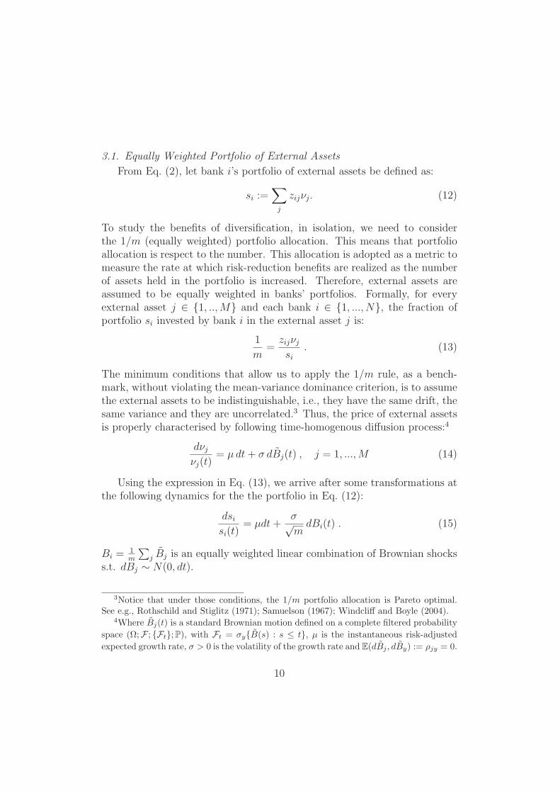
Figure 1: Distribution of portfolio returns (mixture model).

−4 −3 −2 −1 0 1 2 3 40

0.1

0.2

0.3

0.4

0.5

0.6

0.7

0.8

Randomly produced numbers

Dis

trib

utio

ns

componentsmixture modelestimated modelnormal distribution

Comparison between a portfolio with returns following a bimodal distribution (black color)

and a portfolio with normally distributed returns (gray colour). Parameters: μ = 0,

μ− = −1, μ+ = 1, σ = 1, p = 0.5.

Figure 1 illustrates this result by comparing two probability density func-tions (pdf). The first (gray color) curve represents the pdf of a portfoliowith returns X normally distributed, i.e., X ∼ N(0, 1). The second (blackcolor) curve represents the pdf of a portfolio with returns distributed asY 1 ∼ N(0.5, 1) with probability p = 0.5 and as Y 2 ∼ N(−0.5, 1) with prob-ability 1−p = 0.5. Notice that in a world where the market displays a normaldistribution, the middle part of the distribution range (the “belly”) is themost likely outcome. In contrast, in a bimodal world, the belly is the leastlikely outcome. Moreover, the tails of the bimodal distribution are higherthan those of the normal distribution. This indicates the higher probabilityof severe left and right side events. The distance between the two peaks de-pends on the difference between the means of the two normal distributions,|(μ+) − (μ−)|. The (possible) asymmetry between the two peaks and theskewness of the bimodal distribution depends on the difference between the

12

probability of having an uptrend or a downtrend, |(1 − p) − p|. As a re-sult, portfolio diversification choice is subject to much more uncertainty in abimodal world than in a normal one. The next sections show how the statis-tical properties of the bimodal distribution impact on the risk diversificationeffects.

3.2. Systemic Default Probability

Interbank Network structure and Contagion. We leave aside issuesrelated to endogenous interbank network formation, optimal interbank net-work structures and network efficiency. See Leitner (2005), Gale and Kariv(2007), Castiglionesi and Navarro (2007) and the survey by Allen and Babus(2009) for discussion of these topics.

In our analysis, we assume the presence of a tightly knit network of homo-geneous banks holding balance sheets and portfolios that look alike. Indeed,it has been argued that the financial sector has undergone increasing levelsof homogeneity, Haldane (2009). Moreover, empirical evidence shows thatbank networks feature a core-periphery structure with a dense core of fullyconnected banks and a periphery of small banks. Thus, our hypothesis ofhomogeneity is realistic for the banks in the core (see, e.g., Elsinger et al.,2006; Iori et al., 2006; Battiston et al., 2012c).

Despite, one might distinguish between two channels of contagion bywhich shocks may propagate: direct asset price contagion (via overlappingportfolios) and indirect asset price contagion (via interbank claims), strictinterdependencies make it difficult to characterize the propagation of conta-gion in the system. The potential spread of contagion is high and immediate.Since, the size and structure of interbank linkages are hold constant, all thebanks are likely to be hit as defaults propagate through the system.5

Relation between Individual and Systemic Default. Under the prop-erty of homogeneity, banks are assumed to adopt the same capital structure:

- the portfolio of external assets is similar across banks, i.e., si = s forall i ∈ {1, ..., N};- the book value of promised payments at maturity is equal for everybank, i.e., li = l for all i ∈ {1, ..., N}.

5Arguably, it is appropriate to assume that the network remains static, especially indowntrend periods. See Gai and Kapadia (2007).

13

Under those conditions, leverage ratios may differ across banks and over time,but they will remain close to the mean leverage over all banks. Namely, theleverage of every bank “converges” in distribution to the market leverage:

φid 1

N

N∑j

φj := φ ,

for all i ∈ {1, ..., N}. The above assumption, together with the results fromthe previous section allow us to rewrite Eq. (10) as:

φ = l/

(s+

l

1 + rf + βφ

). (17)

which is a quadratic expression in φ:

φ2βs+ φ (sR + l(1− β))− lR = 0 , R = 1 + rf . (18)

Heuristically, we can proof that Eq. (18) has always one positive and onenegative root for any values of the parameters (β > 0, R ≥ 1, s > 0, l > 0)in their range of variation:⎧⎨

⎩φpos = 1

2βs

[l(β − 1)−Rs+

(4βlRs+ (l(1− β) +Rs)2

)1/2],

φneg = 12βs

[l(β − 1)−Rs− (

4βlRs+ (l(1− β) +Rs)2)1/2]

.

Since, by definition φ can only be positive, we exclude the negative solution.Therefore, one can always find a unique positive solution to Eq. (18):

φ := φpos. (19)

14

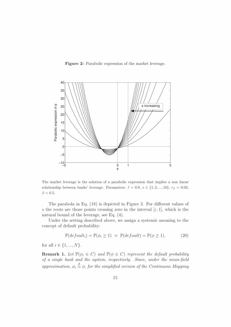
Figure 2: Parabolic expression of the market leverage.

−5 0 1 5−10

−5

0

5

10

15

20

25

30

35

40

φ

Par

abol

ic e

xpre

ssio

n in

φ s increasing

The market leverage is the solution of a parabolic expression that implies a non linear

relationship between banks’ leverage. Parameters: l = 0.9, s ∈ {1, 2, ..., 10}, rf = 0.03,

β = 0.5.

The parabola in Eq. (18) is depicted in Figure 2. For different values ofs the roots are those points crossing zero in the interval [ε, 1], which is thenatural bound of the leverage, see Eq. (4).

Under the setting described above, we assign a systemic meaning to theconcept of default probability:

P(defaulti) = P(φi ≥ 1) P(default) = P(φ ≥ 1), (20)

for all i ∈ {1, ..., N}.Remark 1. Let P(φi ∈ C) and P(φ ∈ C) represent the default probabilityof a single bank and the system, respectively. Since, under the mean-field

approximation, φid φ, for the simplified version of the Continuous Mapping

15

Theorem, P(φi ∈ C) P(φ ∈ C) for all continuity sets C ⊆ Ωφ := [ε, 1] andall i ∈ {1, ..., N}.

P(default) depends on the distribution of φ that, in turn, depends on thedistribution of s. Hence, the systemic default probability can be also definedw.r.t. s:

P(default) = P(φ ≥ 1) ≡ P(s ≤ s−) (21)

with

{s+ = l(βε−ε+1)

(βε2+ε)safe boundary

s− =l(rf+β)

R+βdefault boundary .

See Appendix A. Given the distribution properties of the portfolio in Eq. (16)and the default conditions in Eq.(21), P(default) can be expressed as:

P(default) =

(∫ s+

s0

dsψ(x)

)/

(∫ s+

s−dxψ(x)

), where ψ(x) = exp

(∫ x

0

−2μ

σ2ds

).

(22)

Eq. (22) has the following closed form solution:

P(default) =

(exp

[−2μs0

σ2

]− exp

[−2μs+

σ2

])/

(exp

[−2μs−

σ2

]− exp

[−2μs+

σ2

]).

See Appendix A. Eq. (22) is the probability that s, initially at an arbitrarylevel s(0) := s0 ∈ (s−, s+), exits through s− before s+ after time t > 0. Thiscan be related to the problem of first exit time through a particular end of theinterval (s−, s+), see Gardiner (1985). Now, we define the systemic defaultprobability, conditional to a given trend followed by the external assets, as:{

q := P(default | μ−) def. prob. in the case of a downtrend ,g := P(default | μ+) def. prob. in the case of an uptrend

with the following closed form solutions:⎧⎨⎩

q =(exp

[− (2μ−)s0

σ2/m

]− exp

[− (2μ−)s+

σ2/m

])/(exp

[− (2μ−)s−

σ2/m

]− exp

[− (2μ−)s+

σ2/m

]),

g =(exp

[− (2μ+)s0

σ2/m

]− exp

[− (2μ+)s+

σ2/m

])/(exp

[− (2μ+)s−

σ2/m

]− exp

[− (2μ+)s+

σ2/m

]).

See Appendix A.

16

Figure 3: Conditional Default Prob. for different levels of risk diversification.

0 20 40 60 80 1000

0.1

0.2

0.3

0.4

0.5

0.6

0.7

0.8

0.9

1

diversification (m)

Con

ditio

nal D

efau

lt P

roba

bilit

y

μs+

μ

s−

Conditional def. prob. q given a downtrend (black lines). Conditional def. prob. g

given an uptrend (gray lines). q increases with diversification. Instead, g decreases with

diversification. The elasticity of q and g w.r.t. m depends on the magnitude of the trend.

Parameters: |μ+| = |μ−| ∈ {0.005, 0.01, 0.02, 0.025, 0.03}, l = 0.9, s0 = (s+ − s−)/2,σ = 0.5, rf = 0.01, ε = 0.1, β = 0.2.

Diversification effects on Default Probability.. An asymptotic analy-sis of q and g reveals that, in an idealized world without transaction costs andinfinite population size of external assets (i.e., M → ∞), at increasing levelsof risk diversification (i.e., m → M), the default probability exhibits a bi-furcated behavior. Precisely, g (q) decreases (increases) with diversification.6

See Figure 3. We conclude with the following general proposition:

6In both cases, trends are assumed to be persistent (i.e., approximately constant duringa given period Δt).

17

Proposition 1. Consider a debt-financed portfolio subject to a fix defaultthreshold. Then, the mitigation of idiosyncratic risks via portfolio diversi-fication is desirable when asset prices uptrend and undesirable when assetprices downtrend. The degree of (un)desirability, which is measured in termsof default probability, increases with the level of diversification.

See Appendix A. The intuition behind the polarization of the proba-bility to “survive” and the probability to “fail” is beguilingly simple, butits implications are profound. In brief, the diversification of idiosyncraticrisks reduces the volatility of the portfolio. The lower volatility increases thelikelihood of the portfolio to follow an underlying economic trend. Therefore:

- in uptrend periods, diversification is beneficial because it reduces thedownside risk and highlights the positive trend; thus, the default prob-ability decreases;

- in downtrend periods, diversification is detrimental because it reducesthe upside potential and highlights the negative trend; therefore, thedefault probability increases.

Figure 4 explains this intuition by showing how the pdf of portfolio returns isinfluenced by the downtrend probability and by the level of diversification. Asone may observe, for increasing diversification, viz., lower volatility, the pdfchanges shape by moving from the thick black curve (σ = 0.7), to the mediumblack curve (σ = 0.4), and finally to the thin black curve (σ = 0.2). In Figure4 a) the probability of a positive trend is greater than the probability of anegative trend, p = 0.2. Therefore, diversification is desirable because itreduces the volatility and, by doing so, it shifts to the right the density ofthe distribution of portfolio returns. Instead, In Figure 4 b) the probabilityof a negative trend is greater than the probability of a positive trend, p = 0.8.In this case, diversification is undesirable because, by reducing the volatility,it shifts to the left the density of the distribution.

18

Figure 4: Distribution of portfolio returns for different levels of volatility anddifferent prob. of downtrend.

−4 −2 0 2 40

0.2

0.4

0.6

0.8

1

1.2

1.4

1.6

1.8

2

Randomly produced numbers

Dis

trib

utio

ns

σ = 0.7σ = 0.4σ = 0.2

(a)

−4 −2 0 2 40

0.2

0.4

0.6

0.8

1

1.2

1.4

1.6

1.8

2

Randomly produced numbers

Dis

trib

utio

ns

σ = 0.7σ = 0.4σ = 0.2

(b)

Comparison between the probability density functions of three portfolios with returns

following a bimodal distribution with the same expected value but decreasing volatility.

Thick black curve (σ = 0.7), medium black curve (σ = 0.4), thin black curve (σ = 0.2). (a)

Each curve represents the pdf of a portfolio with returns distributed as Y 1 ∼ N(−0.5, σ)

with probability p = 0.2 and as Y 2 ∼ N(0.5, σ) with probability 1 − p = 0.8. (b) Each

curve represents the pdf of a portfolio with returns distributed as Y 1 ∼ N(0.5, σ) with

probability p = 0.8 and as Y 2 ∼ N(0.5, σ) with probability 1− p = 0.2.

3.3. Bank Utility Function

In this section we formalize the bank utility maximization problem withrespect to the number m of external assets held in the equally weightedportfolio described in Section 3.1.

The bank’s payoff from investing in external assets is a random variableΠm that depends on the number m of external assets in portfolio and ontheir values. It takes the value π in the set Ωπ = [π−, ..., π+], where:{

π− := s− − s0 max attainable profit,π+ := s+ − s0 max attainable loss.

19

More specifically, given m mutually exclusive choices (i.e., the bank portfoliocan be composed of 1, 2, ... external assets) and their corresponding randomreturn Π1,Π2, ..., with distribution function F1(π), F2(π), ..., preferences thatsatisfy the von Neumann-Morgenstern axioms imply the existence of a mea-surable, continuous utility function U(π) such that Π1 is preferred to Π2 ifand only if EU(Π1) > EU(Π2). We assume that banks are mean-variance(MV) decision makers, such that the utility function EU(Πm) may be writ-ten as a smooth function V (E(Πm), σ

2(Πm))7 of the mean E(Πm) and the

variance σ2(Πm) of Πm or

V(E(Πm), σ

2(Πm)):= EU(Πm) = E(Πm)− (λσ2(Πm))/2

such that Π1 is preferred to Π2 if and only if 8

V(E(Π1), σ

2(Π1))> V

(E(Π2), σ

2(Π2)).

Then, the maximization problem is as follows:

maxm

EU(Πm) = E(Πm)− λσ2(Πm)

2(23)

s.t.:

⎧⎪⎪⎨⎪⎪⎩

1 ≤ m ≤Ml > 0s− < s0 < s+

pμ−s + (1− p)μ+

s > 0

with

⎧⎪⎪⎨⎪⎪⎩

E(Πm) = p [qπ− + (1− q)π+] + (1− p) [gπ− + (1− g)π+]

σ2(Πm) = p[q (π− − E(Πm))

2+ (1− q) (π+ − E(Πm))

2]

+(1− p)[g (π− − E(Πm))

2+ (1− g) (π+ − E(Πm))

2].

Notice that Eq.(23) is a static non-linear optimization problem w.r.t. m,with inequality constraints. The first constraint means that m can take onlypositive values between 1 andM . The second constraint requires banks to be

7To describe V as smooth, it simply means that V is a twice differentiable function ofthe parameters E(Πm) and σ2(Πm).

8Only the first two moments are relevant for the decision maker; thus, the ex-pected utility can be written as a function in terms of the expected return (increas-ing) and the variance (decreasing) only, with ∂V

(E(Πm), σ2(Πm)

)/∂E(Πm) > 0 and

∂V(E(Πm), σ2(Πm)

)/∂ σ2(Πm) < 0.

20

debt-financed. The third constraint requires that banks are not yet in defaultwhen implementing their asset allocation, i.e., the initial portfolio value mustlie between the lower default boundary and the upper safe boundary. The lastconstraint represents the “economic growth” condition. That is, the expectedeconomic trend of the real economy-related assets has to be positive. Since bydefinition, |μ−

s |=|μ+s |, this condition is equivalent to impose an upper bound

to the downtrend probability, namely p ∈ Ωp := [0, 12). Then, given the

above constraints, at time t banks randomly select (and fix) the number mof external assets to hold in their portfolio in order to minimize their defaultprobability. This, in turn, maximizes their expected utility.

Figure 5: Expected MV Utility for different levels of risk diversification.

0 20 40 60 80 100−0.2

−0.1

0

0.1

0.2

0.3

0.4

0.5

diversification (m)

Util

ity (

Sys

tem

)

μ = 0.003, s

0 = 4.5

μ = 0.005, s0 = 4.5

μ = 0.003, s0 = 4.0

μ = 0.005, s0 = 4.0

μ = 0.003, s0 = 3.7

μ = 0.005, s0 = 3.7

(a)

0 20 40 60 80 100−0.2

−0.1

0

0.1

0.2

0.3

0.4

0.5

diversification (m)

Util

ity (

Reg

ulat

or)

μ = 0.003, s

0 = 4.5

μ = 0.005, s0 = 4.5

μ = 0.003, s0 = 4.0

μ = 0.005, s0 = 4.0

μ = 0.003, s0 = 3.7

μ = 0.005, s0 = 3.7

(b)

Fixed downtrend probability, p = 0.4. The figure compares the expected MV utility of

the banking system vs. the expected MV utility of the regulator. The curves represent

different initial asset values, s0, and different drifts, μ. (a) Exp. MV Utility of the banking

system EU(Πm). (b) Exp. MV Utility of the regulator EUr(Πm). Parameters: σ2 = 0.5,

rf = 0.001, ε = 0.1, λ = 0.1, β = 0.2, l = 0.5, k = 2, m ∈ {1, ..., 100}, s0 ∈ {3.7, 4, 4.5},|μ+| = |μ−| ∈ {0.003, 0.005}.

21

3.4. Solution of the Bank Max Problem

The analysis of Eq. (23) leads to the following proposition:

Proposition 2. Given the probability interval Ωp := [0, 12), there exists a

subinterval Ωp� ⊂ Ωp s.t., to each p� ∈ Ωp� corresponds an optimal level of di-

versification m� in the open ball B(1+M2, r)=

{m� ∈ R | d

(m�, 1+M

2

)< r

}with center 1+M

2and radius r ∈ [0, α] where α = f(q, g). Then, EU(Πm) ≤

EU(Πm�), for all m /∈ B(1+M2, r).

See Appendix A. Proposition 2 states that optimal diversification maybe an interior solution. Namely, when banks maximize their MV utility theymay choose an intermediate level of diversification, viz., m� ∈ (1,M). m�

is the unique optimal solution and its level depends on the market size andon the likelihood of incurring in a negative or positive trend. In the wordsof Haldane (2009), we show that diversification is a double-edged strategy.Values of m ≷ m� are second-best choices. Precisely, by increasing m to ap-proachm� from below, banks increase their utility. However, by increasingmbeyond m�, banks decrease their utility. In summary, the MV utility exhibitsinverse U-shaped non-monotonic behavior with respect to m. These resultshold under the market structure described in the previous sections. Briefly,banks are fully rational agents with incomplete information about the futurestate of the world. There are no transaction costs, negative externalities ormarket asymmetries. Market returns exhibit a bimodal distribution.

For a fixed probability p, Figure 5 a) shows how the utility changes fordifferent levels of diversification m, different magnitudes of the trend anddifferent initial asset values, s0. Instead, for a fixed initial asset value s0,Figure 6 a) shows how the utility changes for different levels of diversificationm, different magnitudes of the trend and different probability of downtrend,p. Notice that, m enters into the maximization problem via Eq. (15). Inparticular, the portfolio volatility decreases with m. Therefore, an outwardmovement along the x-axis in Figures 5–6, i.e., increasing m, is equivalentto a market condition where the volatility of the assets is low, σ = σlow.Conversely, an inward movement along the x-axis in Figures 5–6, i.e., de-creasing m, is equivalent to a market condition where the volatility of theassets is high, σ = σhigh. To conclude, one might observe that if banks arealready in m�, an abrupt increases in the volatility of the assets (equivalent

22

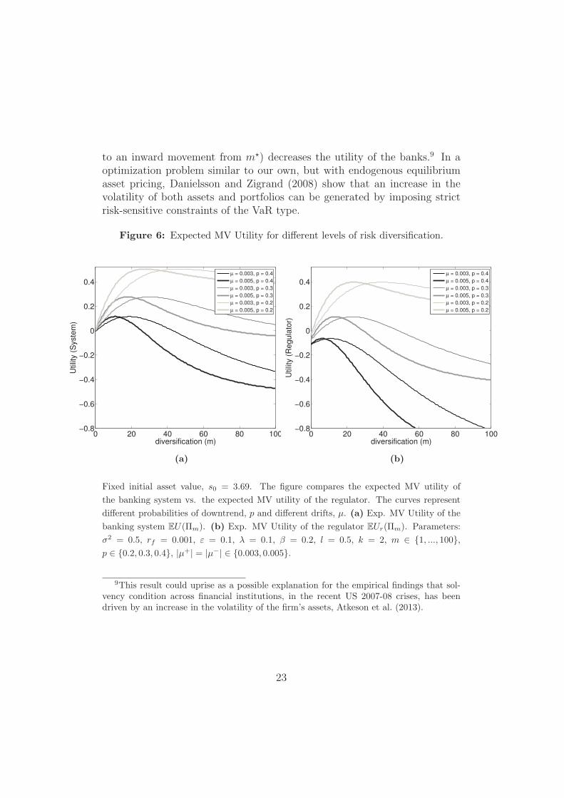
to an inward movement from m�) decreases the utility of the banks.9 In aoptimization problem similar to our own, but with endogenous equilibriumasset pricing, Danielsson and Zigrand (2008) show that an increase in thevolatility of both assets and portfolios can be generated by imposing strictrisk-sensitive constraints of the VaR type.

Figure 6: Expected MV Utility for different levels of risk diversification.

0 20 40 60 80 100−0.8

−0.6

−0.4

−0.2

0

0.2

0.4

diversification (m)

Util

ity (

Sys

tem

)

μ = 0.003, p = 0.4μ = 0.005, p = 0.4μ = 0.003, p = 0.3μ = 0.005, p = 0.3μ = 0.003, p = 0.2μ = 0.005, p = 0.2

(a)

0 20 40 60 80 100−0.8

−0.6

−0.4

−0.2

0

0.2

0.4

diversification (m)

Util

ity (

Reg

ulat

or)

μ = 0.003, p = 0.4μ = 0.005, p = 0.4μ = 0.003, p = 0.3μ = 0.005, p = 0.3μ = 0.003, p = 0.2μ = 0.005, p = 0.2

(b)

Fixed initial asset value, s0 = 3.69. The figure compares the expected MV utility of

the banking system vs. the expected MV utility of the regulator. The curves represent

different probabilities of downtrend, p and different drifts, μ. (a) Exp. MV Utility of the

banking system EU(Πm). (b) Exp. MV Utility of the regulator EUr(Πm). Parameters:

σ2 = 0.5, rf = 0.001, ε = 0.1, λ = 0.1, β = 0.2, l = 0.5, k = 2, m ∈ {1, ..., 100},p ∈ {0.2, 0.3, 0.4}, |μ+| = |μ−| ∈ {0.003, 0.005}.

9This result could uprise as a possible explanation for the empirical findings that sol-vency condition across financial institutions, in the recent US 2007-08 crises, has beendriven by an increase in the volatility of the firm’s assets, Atkeson et al. (2013).

23

4. Private Incentives vs. Social Welfare

Consider a sophisticated bank that, differently from the other banks,internalizes in its maximization problem the social costs due to multiplebank failures. These are negative externalities that limited-liability bankscommonly do not account for. The definition of social losses is rather flexiblesince it depends on the characteristics of the financial system under analysis.In our model, we remain generic regarding the structure of these social costs.

In this section, we formulate the utility maximization problem of thissophisticated bank that we call “regulator” and compare it to the utilitymaximization problem of individual banks in Eq. (23). Let K be the num-ber of simultaneously crashing banks. Then, it is reasonable to assume thefollowings:

Assumption 1. The total loss to be accounted for by the regulator in down-trend periods is a monotonically increasing function f(k, π−) := kπ− of: (i)the expected number k of bank crashes given a collapse of at least one bankE(K|K ≥ 1) = k, (ii) the magnitude of the loss π−.

4.1. Regulator Utility Function

Therefore, the regulator’s utility maximization problem is as follows,

maxm

EUr(Πm) = Er(Πm)− λσ2r(Πm)

2(24)

s.t.:

⎧⎪⎪⎪⎪⎨⎪⎪⎪⎪⎩

1 ≤ m ≤Ml > 0s− < s0 < s+

pμ−s + (1− p)μ+

s > 0k > 1

with

⎧⎪⎪⎨⎪⎪⎩

Er(Πm) = p [qkπ− + (1− q)π+] + (1− p) [gπ− + (1− g)π+]

σ2r(Πm) = p

[q (kπ− − E(Πm))

2+ (1− q) (π+ − E(Πm))

2]

+(1− p)[g (π− − E(Πm))

2+ (1− g) (π+ − E(Πm))

2].

Notice that, with respect to the optimization in Eq. (23), the regulator issubject to the additional constraint k > 1 that amplifies both the expectedloss and its variance. In summary, we compare the general solution of themaximization problem in Eq. (23) with that in Eq. (24).

24

4.2. Results

The analysis shows that the optimal level of diversification for the regu-lator, mr, is left-shifted with respect to the one desirable from the financialsystem point of view, m�. Therefore,

Proposition 3. The incentives of individual banks favor a banking systemthat is over-diversified in external assets w.r.t. to the level of diversificationthat is socially desirable:

m� ≥ mr . (25)

See Appendix A. This result can be also illustrated by comparing Figure 5a) with Figure 5 b) and Figure 6 a) with Figure 6 b).

To conclude, our model suggests that over-diversification occurs becausebanks do not internalize in their utility maximization problem the fact thattheir failure may also drag down other banks causing generalized losses to thewhole system. As a final result, as soon as the probability of downtrend ismoderately high, diversification turns to be a negative strategy that decreasesthe utility of the system.

5. Concluding Remarks

This paper provides a new modeling framework to measure the benefitsthat are associated with holding a diversified portfolio of assets in a systemcontext of banks with interlocked balance sheets. In particular, we use theBlack-Cox first-passage-time approach to measure the default probability ofindividual banks in a network context a‘ la Eisenberg and Noe. Indeed,we model the evolution over time of banks assets as stochastic processeswhere, at the same time, interbank assets value are a function of the financialfragility of the counterparties.

A first contribution of our dynamic and stochastic portfolio approachlies in measuring the benefits of risk diversification not in terms of portfoliovariance but in terms of default probability and expected utility. The advan-tage of the stochastic approach is to provide an ex-ante estimation of defaultprobability as opposed to what is usually done in the works building on theEisenberg-Noe approach.

A second contribution is to compare the optimal diversification at indi-vidual and system levels. In contrast with previous studies, we find thateven in the absence of transaction costs, the optimal level of diversification

25

is interior both for the individuals and the system. The mechanism behindthis result functions as follows. The mitigation of idiosyncratic risks reducesthe volatility of the portfolio of assets in the balance sheet. A lower level ofvolatility reduces the likelihood of the portfolio return to deviate from theunderlying economic trend. Therefore, if the assets in portfolio are trend-ing upward, then increasing diversification is a good strategy that reducesthe default probability and increases the expected utility. Conversely, if theassets are in a downtrend, then increasing diversification is a poor strategythat increases the default probability and reduces the expected utility.

Notice that, to better isolate the effectiveness of diversification in mit-igating idiosyncratic risks to which banks are exposed via external assetsholding, in our setting the interbank diversification is fixed and homoge-nous. However, one could introduce some heterogeneity in the balance sheetstructure and in the portfolio holdings of the banks and answer the questionwhether external diversification and interbank diversification are substitutesor complements.

Overall, an important point stemming from our analysis lies in the recog-nition that the objective of a regulator is not to target a specific diversificationlevel of risk but rather to manage the trade-off between the social losses fromdefaults (because of excessive risk spreading in economic downturn) and thesocial costs of avoiding defaults (because of excessive risk diversification ineconomic booms).

Appendix A. Proofs

Proof. Implicit Recovery Rate The recovery rate is the proportion of face valuethat is recovered through bankruptcy procedures in the event of a default. There-fore, the general formula for the discounted recovery rate δ is

δ =li

(1 + rf + βφi)

(1

li

)(A.1)

=1

(1 + rf + βφi).

That is

δ =

{1

1+rf in case of no default1

1+rf+β in case of default

26

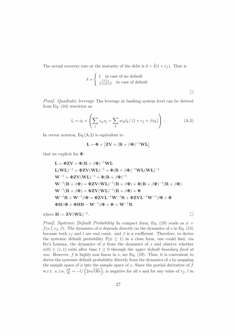
The actual recovery rate at the maturity of the debt is δ = δ(1 + rf ). That is

δ =

{1 in case of no default1+rf

1+rf+β in case of default

Proof. Quadratic leverage The leverage at banking system level can be derivedfrom Eq. (10) rewritten as:

li = φi ×⎛⎝∑

j

zijsj +∑k

wiklk/ (1 + rf + βφk)

⎞⎠ . (A.2)

In vector notaton, Eq.(A.2) is equivalent to

L = Φ× [ZV + (R+ βΦ)−1WL

]that we explicit for Φ:

L = ΦZV +Φ(R+ βΦ)−1WL

L(WL)−1 = ΦZV(WL)−1 +Φ(R+ βΦ)−1WL(WL)−1

W−1 = ΦZV(WL)−1 +Φ(R+ βΦ)−1

W−1(R+ βΦ) = ΦZV(WL)−1(R+ βΦ) +Φ(R+ βΦ)−1(R+ βΦ)

W−1(R+ βΦ) = ΦZV(WL)−1(R+ βΦ) +Φ

W−1R+W−1βΦ = ΦZVL−1W−1R+ΦZVL−1W−1βΦ+Φ

ΦHβΦ+ΦHR−W−1βΦ+Φ = W−1R

where H := ZV(WL)−1.

Proof. Systemic Default Probability In compact form, Eq. (19) reads as φ =f(s, l, rf , β). The dynamics of φ depends directly on the dynamics of s in Eq. (15)because both rf and l are real const. and β is a coefficient. Therefore, to derivethe systemic default probability P(φ ≥ 1) in a close form, one could find, viaIto’s Lemma, the dynamics of φ from the dynamics of s and observe whetherφ(0) ∈ (ε, 1) exits after time t ≥ 0 through the upper default boundary fixed atone. However, f is highly non linear in s, see Eq. (19). Thus, it is convenient toderive the systemic default probability directly from the dynamics of s by mappingthe sample space of φ into the sample space of s. Since the partial derivative of f

w.r.t. s, i.e, ∂f∂s = −l/

(2s√lRs

), is negative for all s and for any value of rf , l in

27

their range of variation, the Inverse Function Theorem implies that f is invertibleon R

+:

f−1(φ) =l(2φ+R)

φ(φ+R), s.t. (f−1)′(φ) =

1

f ′(s).

Observe that, by definition, the value of external assets cannot be negative, s ∈ R+.

The partial derivative f ′(s) w.r.t. s is negative for all s and for any value of (l, rf ,β) in their range of variation:

f ′(s) =−l

((β − 1)2l + (1 + β)Rs+ (−1 + β)

√(−1 + β)2l2 + 2(1 + β)pRs+R2s2

)2βs2

√4βlRs(l − βl +Rs)2

< 0

Then, by the Inverse Function Theorem f is invertible on R+

f−1(φ) =l(φ+ βφ+R)

φ(βφ+R), s.t. (f−1)′(φ) =

1

f ′(y).

Moreover, one can show that the inverse f−1 is continuous. Given the above result,we obtain the following mapping between the values of φ and s:{

f(s) = 1 iff f−1(φ) =l(rf+β)(R+β) := s−

f(s) = ε iff f−1(φ) = l(βε−ε+1)(βε2+ε)

:= s+ .

Hence, the systemic default probability can be defined also w.r.t. s:

P(default) = P(φ ≥ 1) ≡ P(s ≤ s−).

This is the probability that s, initially at an arbitrary level s(0) := s0 ∈ (s−, s+),exits through the lower default boundary s− after time t ≥ 0. From Gardiner(1985), P(s ≤ s−) has the following explicit form:

P(s ≤ s−) =

(∫ s+

s0

dsψ(x)

)/

(∫ s+

s−dxψ(x)

). (A.3)

with ψ(x) = exp(∫ x

0 −2μσ2 ds

). Eq. (A.3) has the following closed form solution:

P(s ≤ s−) =(exp

[− 2μs0

σ2

]− exp

[− 2μs+

σ2

])/

(exp

[− 2μs−

σ2

]− exp

[− 2μs+

σ2

]),

(A.4)

with μ = pμ++(1−p)μ− and σ2 = p[(μ+ − μ)2 + σ2

m

]+(1−p)

[(μ− − μ)2 + σ2

m

].

During a downtrend, Eq. (A.3) yields the conditional default probability given adowntrend

q := P(default | μ−) = P(s ≤ s− | μ−)

28

with the following closed form solution:

q =

(exp

[− (2μ−)s0

σ2/m

]− exp

[− (2μ−)s+

σ2/m

])/

(exp

[− (2μ−)s−

σ2/m

]− exp

[− (2μ−)s+

σ2/m

]).

(A.5)During an uptrend, Eq. (A.3) yields the conditional default probability given anuptrend:

g := P(default | μ+) = P(s ≤ s− | μ+)with the following closed form solution:

g =

(exp

[− (2μ+)s0

σ2/m

]− exp

[− (2μ+)s+

σ2/m

])/

(exp

[− (2μ+)s−

σ2/m

]− exp

[− (2μ+)s+

σ2/m

]).

(A.6)

Proof. Bifurcation of the conditional default probabilityWe provide an asymptotic analysis that explains the results presented in Propo-

sition 1. Let rewrite Eq. (A.5) and Eq. (A.6) as

q =M s0

(−) −M s+

(−)

M s−(−) −M s+

(−)

=M(s0−s+)(−)

[M

(s−−s+)(−) − 1

]− 1

M(s−−s+)(−) − 1

(A.7a)

g =M s0

(+) −M s+

(+)

M s−(+) −M s+

(+)

=M(s0−s+)(+)

[M

(s−−s+)(+) − 1

]− 1

M(s−−s+)(+) − 1

(A.7b)

withM(−) = exp[−(2μ−)m

σ2

]andM(+) = exp

[−(2μ+)mσ2

]. Then, the following result

is straightforward: {lim

m→+∞ q = 0− (−1) = 1

limm→+∞ g = 0− 0 = 0

To conclude, for any arbitrary small number ε ∈ (0, 1)

∃ m > 1 | (q − g) > 1− ε ∀ m > m

29

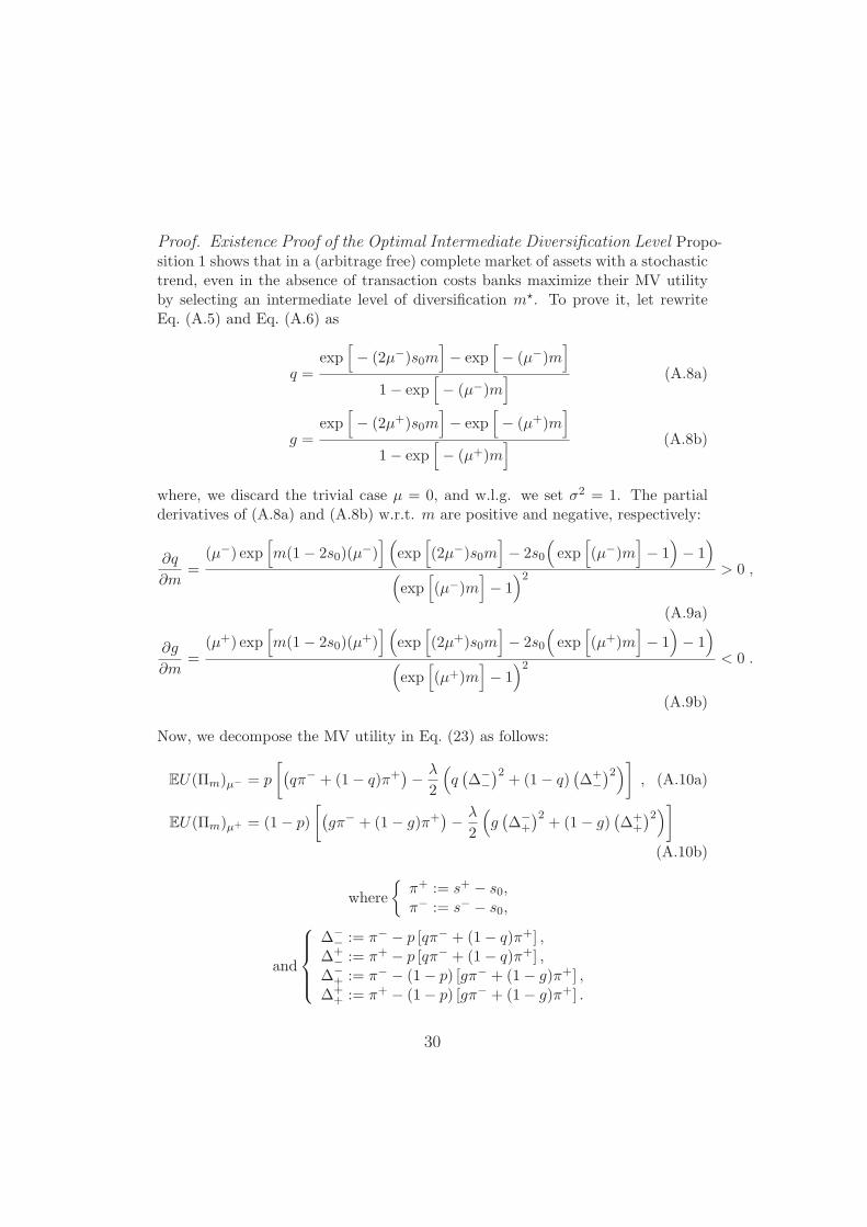
Proof. Existence Proof of the Optimal Intermediate Diversification Level Propo-sition 1 shows that in a (arbitrage free) complete market of assets with a stochastictrend, even in the absence of transaction costs banks maximize their MV utilityby selecting an intermediate level of diversification m�. To prove it, let rewriteEq. (A.5) and Eq. (A.6) as

q =exp

[− (2μ−)s0m

]− exp

[− (μ−)m

]1− exp

[− (μ−)m

] (A.8a)

g =exp

[− (2μ+)s0m

]− exp

[− (μ+)m

]1− exp

[− (μ+)m

] (A.8b)

where, we discard the trivial case μ = 0, and w.l.g. we set σ2 = 1. The partialderivatives of (A.8a) and (A.8b) w.r.t. m are positive and negative, respectively:

∂q

∂m=

(μ−) exp[m(1− 2s0)(μ

−)] (

exp[(2μ−)s0m

]− 2s0

(exp

[(μ−)m

]− 1

)− 1

)(exp

[(μ−)m

]− 1

)2 > 0 ,

(A.9a)

∂g

∂m=

(μ+) exp[m(1− 2s0)(μ

+)] (

exp[(2μ+)s0m

]− 2s0

(exp

[(μ+)m

]− 1

)− 1

)(exp

[(μ+)m

]− 1

)2 < 0 .

(A.9b)

Now, we decompose the MV utility in Eq. (23) as follows:

EU(Πm)μ− = p

[(qπ− + (1− q)π+

)− λ

2

(q(Δ−

−)2

+ (1− q)(Δ+

−)2)]

, (A.10a)

EU(Πm)μ+ = (1− p)

[(gπ− + (1− g)π+

)− λ

2

(g(Δ−

+

)2+ (1− g)

(Δ+

+

)2)](A.10b)

where

{π+ := s+ − s0,π− := s− − s0,

and

⎧⎪⎪⎨⎪⎪⎩

Δ−− := π− − p [qπ− + (1− q)π+] ,

Δ+− := π+ − p [qπ− + (1− q)π+] ,

Δ−+ := π− − (1− p) [gπ− + (1− g)π+] ,

Δ++ := π+ − (1− p) [gπ− + (1− g)π+] .

30

Let observe that Eq. (A.10a) is decreasing in m, while Eq. (A.10b) is increasingin m:

∂EU(Πm)μ−

∂m= p

(∂q

∂m

)(π− − π+

)< 0 (A.11a)

∂EU(Πm)μ+

∂m= (1− p)

(∂g

∂m

)(π− − π+

)> 0 (A.11b)

Eq. (23) can be interpreted as a linear combination of Eq. (A.10a) and Eq. (A.10b)that are weighted by p and (1 − p), respectively. Then, when the partial deriva-tive in Eq. (A.11a) is equal to the partial derivative in Eq. (A.11b), EU(Πm) ismaximized w.r.t. m. The condition to be verified is to find the probability p� thatmakes the two equations to be equivalent:

FOC: p

(∂q

∂m

)(π− − π+

)= (1− p)

(∂g

∂m

)(π− − π+

).

The condition is satisfied for all

p� = 1/

(1 +

∂q

∂g

)∈ Ωp� ⊂ ΩP := [0, 1] (A.12)

with q = q(m�), g = g(m�). In a more general form, Eq. (A.12) can be writtenas p� = f [g(m�); q(m�)]. Since g, q and f are all one-to-one, for the InversionFunction Theorem are invertible functions. Hence, for a fixed value of p�, mustexists an m� such that:

m� =[(g−1; q−1) ◦ f−1

](p�) ⇒ ∃ EU(Πm�) ≥ EU(Πm) ∀m ≷ m�.

The economic growth condition implies p� < 12 . From (A.12), this is equivalent

to write:

1

2>

∂g∂m

∂q∂m + ∂g

∂m

∂g

∂m<

1

2

[ ∂q∂m

+∂g

∂m

]∂g

∂m+∂g

∂m<

∂q

∂m+∂g

∂m∂g

∂m<

∂q

∂m

which is always true because from Eq. (A.9a)–(A.9b) ∂g∂m < 0 and ∂q

∂m > 0. Toconclude, to each p� ∈ Ωp� ⊂ Ωp := [0, 12) corresponds an optimal level of diver-

sification m� in the open ball B(1+M2 , r

)=

{m� ∈ R | d

(m�, 1+M

2

)< r

}with

31

center 1+M2 and radius r ∈ [0, α] where α = f(q, g). Then, EU(Πm) ≤ EU(Πm�),

for all m /∈ B(1+M2 , r

).

Proof. Banks are Over-Diversified: m� ≥ mr. Following the same line ofreasoning used in the previous proof, we decompose EUr(Πm) as follows:

EUr(Πm)μ− = p

[(qkπ− + (1− q)π+

)− λ

2

(q(kΔ−

−)2

+ (1− q)(Δ+

−)2)]

(A.13a)

EUr(Πm)μ+ = (1− p)

[(gπ− + (1− g)π+

)− λ

2

(g(Δ−

+

)2+ (1− g)

(Δ+

+

)2)].

(A.13b)

Eq. (A.13b) is not affected by Assumption 1 in Section 4 and remains equivalentto (A.10b). Hence, the partial derivative w.r.t. m of Eq. (A.13b) is equal toEq (A.11b):

∂EUr(Πm)μ+

∂m≡ ∂EU(Πm)μ+

∂m= (1− p)

(∂g

∂m

)(π− − π+

).

However, because of the factor k, the partial derivative w.r.t. m of Eq. (A.13a) issteeper than Eq (A.11a) . It is easy to see that for any k > 1,

∂EUr(Πm)μ−

∂m= p

(∂q

∂m

)(kπ− − π+

)<∂EU(Πm)μ−

∂m= p

(∂q

∂m

)(π− − π+

)< 0

The condition to be verified is to find the probability pr that makes the twoequations to be equivalent:

FOC: (1− p)

(∂g

∂m

)(π− − π+

)= p

(∂q

∂m

)(kπ− − π+

).

Discarding the trivial solution μs = 0, the condition is satisfied for all

pr = 1/

(1 +

(∂q

∂g

)υ

)∈ ΩP r ⊂ ΩP := [0, 1] (A.14)

with q = q(mr), g = g(mr) and υ = (kπ−−π+)(π−−π+)

.

In a more general form, (A.14) can be written as

pr = f (υ[g(m�); q(m�)]) .

32

Since g, q, υ and f are all one-to-one and hence invertible functions, for a fixedvalue of pr, must exists an mr such that

mr =[(g−1; q−1) ◦ υ− ◦ f−1

](pr).

Eq.(A.14) is a decreasing function w.r.t. υ which is a constant function biggerthan one because k > 1. Then, pr < p�. This implies that the diversification levelmr is lower than the level m�:

mr =[(g−1; q−1) ◦ υ−1 ◦ f−1

](pr) < m� =

[(g−1; q−1) ◦ f−1

](p�)

Atkeson, A. G., Eisfeldt, A. L., and Weill, P.-O. (2013). Measuring the finan-cial soundness of us firms 1926-2012. Federal Reserve Bank of MinneapolisResearch Department Staff Report 484.

Battiston, S., Delli Gatti, D., Gallegati, M., Greenwald, B. C. N., andStiglitz, J. E. (2012a). Credit Default Cascades: When Does Risk Diver-sification Increase Stability? Journal of Financial Stability, 8(3):138–149.

Battiston, S., Gatti, D. D., Gallegati, M., Greenwald, B. C. N., and Stiglitz,J. E. (2012b). Liaisons Dangereuses: Increasing Connectivity, Risk Shar-ing, and Systemic Risk. J. Economic Dynamics and Control, 36(8):1121–1141.

Battiston, S., Puliga, M., Kaushik, R., Tasca, P., and Caldarelli, G. (2012c).Debtrank: Too central to fail? financial networks, the fed and systemicrisk. Sci. Rep., 2(541).

Bird, R. and Tippett, M. (1986). Naive Diversification and Portfolio Risk-ANote. Management Science, pages 244–251.

Black, F. and Cox, J. (1976). Valuing Corporate Securities: Some Effects ofBond Indenture Provisions. The Journal of Finance, 31(2):351–367.

Brock, W., Hommes, C., and Wagener, F. (2009). More hedging instrumentsmay destabilize markets. Journal of Economic Dynamics and Control,33(11):1912–1928.

Danielsson, J. and Zigrand, J.-P. (2008). Equilibrium asset pricing withsystemic risk. Economic Theory, 35(2):293–319.

33

Cifuentes, R., Ferrucci, G., and Shin, H. S. (2005). Liquidity risk and conta-gion. Journal of the European Economic Association, 3(2-3):556–566.

Collin-Dufresne, P., Goldstein, R. S., and Martin, J. S. (2001). The determi-nants of credit spread changes. The Journal of Finance, 56(6):2177–2207.

Eisenberg, L. and Noe, T. (2001). Systemic risk in financial systems. Man-agement Science, 47(2):236–249.

Elsinger, H., Lehar, A., and Summer, M. (2006). Risk Assessment for Bank-ing Systems. Management Science, 52(9):1301–1314.

Elton, E. J. and Gruber, M. J. (1977). Risk reduction and portfolio size: Ananalytical solution. The Journal of Business, 50(4):pp. 415–437.

Evans, J. and Archer, S. (1968). Diversification and the reduction of disper-sion: an empirical analysis. The Journal of Finance, 23(5):761–767.

Fricke, D. and Lux, T. (2012). Core-periphery structure in the overnightmoney market: Evidence from the e-mid trading platform. Technical re-port, Kiel Working Papers.

Gai, P. and Kapadia, S. (2007). Contagion in financial networks. Bank ofEngland, Working Paper.

Gardiner, C. W. (1985). Handbook of stochastic methods for physics, chem-istry, and the natural sciences. Springer.

Goldstein, I. and Pauzner, A. (2004). Contagion of self-fulfilling financialcrises due to diversification of investment portfolios. Journal of EconomicTheory, 119(1):151–183.

Haldane, A. (2009). Rethinking the financial network. Speech delivered atthe Financial Student Association, Amsterdam, April.

Ibragimov, R., Jaffee, D., and Walden, J. (2011). Diversification disasters.Journal of Financial Economics, 99(2):333–348.

Iori, G., Jafarey, S., and Padilla, F. (2006). Systemic risk on the interbankmarket. Journal of Economic Behaviour and Organization, 61(4):525–542.

34

Johnson, K. and Shannon, D. (1974). A note on diversification and thereduction of dispersion. Journal of Financial Economics, 1(4):365–372.

Mainik, G. and Embrechts, P. (2012). Diversification in heavy-tailed portfo-lios: properties and pitfalls. Annals Actuarial Science, to appear.

Markowitz, H. (1952). Portfolio selection. The Journal of Finance, 7(1):77–91.

Merton, R. (1974). On the Pricing of Corporate Debt: The Risk Structureof Interest Rates. The Journal of Finance, 29(2):449–470.

Rothschild, M. and Stiglitz, J. E. (1971). Increasing risk ii: Its economicconsequences. Journal of Economic Theory, 3(1):66–84.

Roukny, T., Bersini, H., Pirotte, H., Caldarelli, G., and Battiston, S. (2013).Default Cascades in Complex Networks: Topology and Systemic Risk.Scientific Reports, 3.

Samuelson, P. A. (1967). General proof that diversification pays. The Journalof Financial and Quantitative Analysis, 2(1):pp. 1–13.

Shin, H. (2008). Risk and Liquidity in a System Context. Journal of FinancialIntermediation, 17:315–329.

Statman, M. (1987). How many stocks make a diversified portfolio? TheJournal of Financial and Quantitative Analysis, 22(03):353–363.

Stiglitz, J. (2010). Risk and global economic architecture: Why full finan-cial integration may be undesirable. The American Economic Review,100(2):388–392.

Tobin, J. (1958). Liquidity preference as behavior towards risk. The Reviewof Economic Studies, 25(2):66–86.

Wagner, W. (2009). Diversification at financial institutions and systemiccrises. Journal of Financial Intermediation.

Wagner, W. (2011). Systemic liquidation risk and the diversitydiversificationtradeoff. The Journal of Finance, 66(4):1141–1175.

35

Windcliff, H. and Boyle, P. (2004). The 1/n pension investment puzzle. NorthAmerican Actuarial Journal, 8:32–45.

Zhou, C. (2010). Dependence structure of risk factors and diversificationeffects. Insurance: Mathematics and Economics, 46(3):531–540.

36